Dynamic Modeling of Cable Towed Body using Nodal Position Finite Element Method

Ocean Engineering 38 (2011) 529–540

Contents lists available at ScienceDirect

Ocean Engineering

0029-80

doi:10.1

n Corr

E-m

journal homepage: www.elsevier.com/locate/oceaneng

Dynamic modeling of cable towed body using nodal position finiteelement method

F.J. Sun a, Z.H. Zhu a,n, M. LaRosa b

a Department of Earth and Space Science and Engineering, York University, 4700 Keele Street, Toronto, Ontario, Canada M3J 1P3b Curtiss-Wright Flow Control Company, Indal Technologies, 3570 Hawkestone Road, Mississauga, Ontario, Canada L5C 2V8

a r t i c l e i n f o

Article history:

Received 1 July 2010

Accepted 13 November 2010

Editor-in-Chief: A.I. Incecikdirectly instead of the displacement by the existing finite element method. The newly derived nodal

position finite element method eliminates the need of decoupling the rigid body motion from the total

Keywords:

Nodal position finite element method

Dynamics

Cable

Towed body

Modeling

18/$ - see front matter & 2010 Elsevier Ltd. A

016/j.oceaneng.2010.11.016

esponding author. Tel.: +1 416 736 2100x777

ail address: [email protected] (Z.H. Zhu).

a b s t r a c t

This paper analyses nonlinear dynamics of cable towed body system. The cable has been modeled and

analyzed using a new nodal position finite element method, which calculates the position of the cable

motion, where numerical errors arise in the existing nonlinear finite element method, and the limitation

of small rotation in each time step in the existing nonlinear finite element method. The towed body is

modeled as a rigid body with six degrees of freedom while the tow ship motion is treated as a moving

boundary to the system. A special procedure has been developed to couple the cable element with the

towed body. The current approach can be used as design tool for achieving improved directional stability,

maneuverability, safety and control characteristics with the cable towed body. The analysis results show

the elegance and robustness of the proposed approach by comparing with the sea trial data.

& 2010 Elsevier Ltd. All rights reserved.

1. Introduction

The submerged cable towed body has a wide range of applica-tions in science, industry and defense. Due to the extreme complex-ity of the system, the stability, maneuverability, safety and controlcharacteristics of a specific cable towed body usually cannot befully evaluated until it has been constructed and actually inoperation (Duvat and Large, 1997). To reduce the high riskassociated with design of cable towed body system, computersimulation of the cable towed body has been widely used (Zhu andMorrow, 1998). In these analyses, the towed body is modeled as arigid body with six degrees of freedom (DOF) and the hydrody-namic loads acting on the body are represented by a set ofdimensionless hydrodynamic coefficients that can be determinedexperimentally by towing the towed body in water tank withspecified motions. The ship motion is assumed independent to thetow cable and the towed body because the ship’s mass is severalorders of magnitude higher than the cable and towed body. It istreated as a moving boundary condition of the cable towed bodysystem. The ship connects to the towed body by a cable, which isusually simplified as a flexible tension member and its bendingstiffness is neglected because of the extremely large ratio of lengthover cross-section dimension (Zhu et al., 2003). The motion of thecable involves large rigid body rotation and displacement coupledwith small elastic stretch. In practice, the engineers and designers

ll rights reserved.

29; fax: +1 416 736 5817.

are interested in the current position not the displacement of cable.This leads to the existing analyses of the cable dynamics are mostlydone by finite difference method (FDM) that approximates thegoverning equations of cable by difference equations along thecable with its position as state variable (Koh et al., 1999; Burgess,1999; Koh and Rong, 2004), although finite element method (FEM)is used in some cases (Webster, 1995). For instance, Ablow andSchechter (1983) developed a fully three-dimensional code tocompute the motion of a towed cable based on a robust and stablefinite difference approximation. Huang (1994) modeled the cablebased upon the lump-mass-and-spring model and the finitedifference method. Actually, the lump-mass-and-spring methodis a special case of finite element method using 2-noded straightbar element. However, the FDM is problem specific, which is hardto be implemented in general-purpose analysis programs in analgorithm fashion.

The FEM discretizes the continuous cable into a finite number ofelements. Each element may have different geometrical andmaterial properties but the governing mathematic equations foreach element are the same. By assembling all the elementstogether, the complex geometries with multiple cable branchesor different cable properties along the length can be easily modeledalgorithmically (Zhu et al., 2003). Although the FEM has been usedvirtually in all areas of engineering, it is not widely adopted in theanalysis of cable dynamics because the existing FEM calculatesthe relative displacement not the position of the cable. Instead, thecable’s current position has to be obtained by adding the relativedisplacement to its previous position. In addition, the existing FEMalso requires decoupling the large rigid body displacement and

F.J. Sun et al. / Ocean Engineering 38 (2011) 529–540530

rotation from the small elastic stretch. This process is inconvenientfor the engineers and designers in the field and is prone to theaccumulated numerical errors arising from each time step over along period time. For instance, the large rigid body rotation of thecable leads to geometrical nonlinearity, improper approximation incalculating the strain energy of element based on displacementapproach will result in numerical errors that do not exist in FDM,where the strain is calculated by comparing the current config-uration with original configuration directly. For instance, let usconsider a 2-noded straight cable/bar element experiencing a rigidbody rotation and translation as shown in Fig. 1. The rigid bodydisplacements of any point along the element can be expressed as

u¼ u1þxðcosy�1Þ, v¼ v1þxsiny ð1Þ

Accordingly, the Green–Lagrangian strain of the element iscalculated by

e¼ eLþeN ¼@u

@xþ

1

2

@u

@x

� �2

þ@v

@x

� �2" #

ð2Þ

where

eL ¼@u

@x¼ cosy�1 and eN ¼

1

2

@u

@x

� �2

þ@v

@x

� �2" #

¼1

2ðcosy�1Þ2þsin2yh i

The strain energy of the element is then calculated as

U ¼1

2

Z L

0EAe2ds¼

1

2

Z L

0EAðe2

Lþ2eLeNþe2NÞds¼ 0

The higher order term e2N in the strain energy is commonly

ignored in the existing FEM if one assumes small strain andmoderate rotation, such that

U ¼1

2

Z L

0EAe2ds¼

1

2

Z L

0EAðe2

L þ2eLeNþe2NÞds�

1

2

Z L

0EAðe2

Lþ2eLeNÞds

ð3Þ

From Eq. (3), one can derive the linear stiffness matrix from thefirst term e2

L and the geometric nonlinear stiffness matrix from thesecond term eLeN.

Now let us substitute the rigid body displacement in Eq. (1) intothe approximated strain energy expression in Eq. (3). It shows thestrain energy is not zero as it should be, such that

U �1

2

Z L

0EAðe2

Lþ2eLeNÞds¼�1

2EALðcosy�1Þ2 ð4Þ

Eq. (4) indicates that the existing FE approximation will result inspurious strain energy in dealing with rigid body rotation. Thespurious energy will approach zero only if we assume the rigidbody rotation is small, such that:

cosy� 1

Then, the strain energy in Eq. (4) becomes zero approximately.Thus, it is clear that the FE approximation is valid only for the smallrotation or small increment when the large rigid body rotation isanalyzed by an incremental solution. This tiny approximation error

x

P

θ

v

v

u2v1

u1

P0 u

v

1

L

2Undeformed

v1 P0 u

L

Fig. 1. Schematic of a 2-noded straight cable element experiencing rigid body

motion.

accumulates at each time step and may lead to spurious results dueto violation of energy conservation of the FE model (Simo et al.,1992) over a long period. Many efforts have been devoted to thisproblem in the literature, e.g., the symplectic numerical integratorto ensure the energy conservation of the discretized system (Simoet al., 1992; Tuwankotta and Quispel, 2003). These methods areusually complicated in mathematics. Different to the efforts thatenhances the existing displacement based FEM, some efforts havebeen devoted to develop an alternative finite element procedure tosolve the positions of a system directly after realizing that thepositions are the main interest for certain applications. Forinstance, Shabana (1998) developed an absolute nodal coordinatefinite element method to solve the positions and the slopes of abeam directly.

The current study is motivated by the need of an alternativerobust FEM to the existing FDM/FEM for the dynamic analysis ofcable experiencing large rigid body rotations coupled with smallelastic deformation over a long period. A new FEM has beendeveloped to solve the position of cable directly by re-formulatingthe existing FEM in terms of nodal position instead of nodaldisplacement. Thus, the new nodal position finite element method(NPFEM) will eliminate (i) the need to decouple the rigid bodyrotation and the elastic deformation of element involving largerigid body rotation and (ii) the accumulation errors arising from thenumerical solution process at each time step.

The new NPFEM has been implemented into a simulationprogram together with the rigid body dynamics of the towed bodyand the ship motion as moving boundary condition. The simulationprogram has been developed for the purpose of aiding engineers,designers and operators to achieve improved directional stability,maneuverability, safety and control characteristics of the cabletowed body system. The analysis results demonstrate the eleganceand robustness of the new approach and the credibility of thesimulation program is verified by the sea trial data.

2. Formulation of nodal position finite element method

Most problems of dynamics can be recast in a framework ofgeneralized energetic principles. We will derive the governingequations of nodal position finite element method using theprinciple of virtual work. Consider a two-noded straight cableelement in a three-dimensional space. The element geometry isdescribed by its nodal coordinates (Xi, Yi, Zi) (i¼1, 2) in a globalcoordinate system OXYZ and (xi, yi, zi) (i¼1, 2) in a local coordinatesx, y and z where x-axis is defined along the cable, y- and z-axes areperpendicular to the x-axis, respectively.

Assume the position, velocity and acceleration of an arbitrarypoint along the cable element are expressed in terms of elementshape functions and the corresponding nodal values, such that

R¼NXe, v¼ _R ¼N _X e, a¼ €R ¼N €X e ð5Þ

N ¼

1�z 0 0 z 0 0

0 1�z 0 0 z 0

0 0 1�z 0 0 z

264

375

z¼

ffiffiffiffiffiffiffiffiffiffiffiffiffiffiffiffiffiffiffiffiffiffiffiffiffiffiffiffiffiffiffiffiffiffiffiffiffiffiffiffiffiffiffiffiffiffiffiffiffiffiffiffiffiffiffiffiffiffiffiffiffiffiðX�X1Þ

2þðY�Y1Þ

2þðZ�Z1Þ

2qffiffiffiffiffiffiffiffiffiffiffiffiffiffiffiffiffiffiffiffiffiffiffiffiffiffiffiffiffiffiffiffiffiffiffiffiffiffiffiffiffiffiffiffiffiffiffiffiffiffiffiffiffiffiffiffiffiffiffiffiffiffiffiffiffiffiffiðX2�X1Þ

2þðY2�Y1Þ

2þðZ2�Z1Þ

2q

where R¼{X, Y, Z}T, v¼{vx, vy, vz}T and a¼{ax, ay, az}

T are theposition, velocity and acceleration vectors of the arbitrary point inthe global coordinate system, respectively, Xe¼{X1, Y1, Z1, X2, Y2,Z2}T is the global nodal coordinates at the current time, N is theelement shape function matrix and the dot denotes the timederivations, respectively.

F.J. Sun et al. / Ocean Engineering 38 (2011) 529–540 531

The elastic strain of the element is calculated with respect to theundeformed element length L0, such as

ex ¼L

L0�1¼

L2

L0L�1

¼X2�X1

L0cosyxþ

Y2�Y1

L0cosyyþ

Z2�Z1

L0cosyz�1¼ B0QXe�1

ð6Þ

cosyx ¼X2�X1

Lcosyy ¼

Y2�Y1

Lcosyz ¼

Z2�Z1

Lð7Þ

B0 ¼ �1L , 0, 0, 1

L , 0, 0h i

Q ¼

cosyx cosyy cosyz 0 0 0

0 0 0 0 0 0

0 0 0 0 0 0

0 0 0 cosyx cosyy cosyz

0 0 0 0 0 0

0 0 0 0 0 0

2666666664

3777777775

where L¼ffiffiffiffiffiffiffiffiffiffiffiffiffiffiffiffiffiffiffiffiffiffiffiffiffiffiffiffiffiffiffiffiffiffiffiffiffiffiffiffiffiffiffiffiffiffiffiffiffiffiffiffiffiffiffiffiffiffiffiffiffiffiffiffiffiffiffiðX2�X1Þ

2þðY2�Y1Þ

2þðZ2�Z1Þ

2q

is the length of the

deformed element.It should be noted that the strain matrix B0 is the same as the

existing two-noded cable/bar element and Q is the coordinatetransformation matrix from local to global coordinates.

Based on Eq. (6), the strain energy of element can be expressedas

U ¼1

2

Z L

0EAe2

x ds¼1

2XT

e KXe�XTe Fkþ

1

2EAL ð8Þ

where E is Young’s modulus of the cable, A is the cross sectionarea of the cable, K is the stiffness matrix of element in the globalcoordinate system and Fk is the equivalent nodal force vectorresulting from the elasticity of the cable, such as

K ¼ EALðB0Q ÞT B0Q ¼Q T K0Q ð9Þ

K0 ¼EAL

L20

1 0 0 �1 0 0

0 0 0 0 0 0

0 0 0 0 0 0

�1 0 0 1 0 0

0 0 0 0 0 0

0 0 0 0 0 0

2666666664

3777777775

Fk ¼ EALQ T BT0

It should be noted that the stiffness matrix is similar to thestiffness of the existing two-node straight cable/bar elementsexcept the scaling factor L/L0. For the small strain deformation,L/L0¼1+exE1. Then, the stiffness matrix K0 is the same as theexisting two-node straight cable/bar elements. However, theNPFEM has an extra equivalent nodal elastic force vector Fk thatdoes not exist in the existing FEM. This is not the external load. Itresults from transforming the state variables from nodal displace-ment to nodal position and is the function of element rigidity EA

and orientation only. The K and Fk are highly nonlinear and time-dependent as the coordinate transformation matrix Q is thefunction of the orientation of cable element that varies in time.

Moreover, there is no geometric (or initial stress) stiffnessmatrix commonly existing in the displacement based finite ele-ment method in Eq. (9). The geometric stiffness matrix is due to therigid body rotation when using the nodal displacement to calculatethe strain energy of element. As indicated in the introductionsection, it is the source of accumulation error in case of large rigidbody rotation. The current approach calculates the strain energydirectly by comparing the new element length to its undeformedone using the nodal position. Thus, it eliminates the source of

accumulation error due to large rigid body rotation and, therefore,there is no geometric stiffness matrix in NPFEM formulation.

The kinetic energy of the element can be calculated straightfor-ward, such that

T ¼1

2

Z L

0rz _RT

U _Rdx¼1

2_X T

e M _X e ð10Þ

M ¼rAL

6

2 0 0 1 0 0

0 2 0 0 1 0

0 0 2 0 0 1

1 0 0 2 0 0

0 1 0 0 2 0

0 0 1 0 0 2

2666666664

3777777775

ð11Þ

where M is the mass matrix of the cable element in the globalcoordinate system and r is the material density of the cable. Itshould be noted that the element mass matrix is constant in theglobal coordinate system if LEL0 and is the same as the consistentmass matrix of cable element in the existing FEM.

Once the strain and kinetic energy of element has beencalculated, we need to determine the work done by the externalforces acting on the element. The cable moves in a fluid willexperience the drag and the inertial force due to the added mass offluid (Zhu and Meguid, 2006), such that

f dn ¼�CdnðaÞr0D

2V2 Vn

9Vn9f dt ¼�CdtðaÞ

r0D

2V2 Vt

9Vt9ð12aÞ

f a ¼�Cmr0A _V n ð12bÞ

V ¼ _r�Vc Vt ¼ ðt0UVÞt0 Vn ¼V�Vt ð12cÞ

where fdn and fdt are the drag force components normal and tangentto the cable, respectively, Cdn(a) and Cdt(a) are the normal andtangent drag coefficients, respectively, a is the angle of attack, r0 isthe fluid density, D is the cable diameter, fa is the inertial forcenormal to the cable resulting from the added mass of fluidsurrounding the cable, Cm is the added mass coefficient of thecable, Vc is the free stream velocity of the fluid and t0 is the unitvector along the axis of element.

The inertial force of the added mass is a distributed load actingon the element and the virtual work done by the inertial force isgiven by

dWa ¼�

Z L

0f T

aUdRdx¼ dXTe Ma

€X e�dXTe Fa ð13Þ

Ma ¼Cmr0AL

6ðMa0�Ma1Þ Fa ¼Ma

_V ec ð14aÞ

Ma0 ¼2I3�3 I3�3

I3�3 2I3�3

" #Ma1 ¼

2m0 m0

m0 2m0

" #ð14bÞ

m0 ¼

cos2yx cosyxcosyy cosyxcosyz

cosyxcosyy cos2yy cosyycosyz

cosyxcosyz cosyzcosyy cos2yz

264

375 ð14cÞ

where Ma is the added mass matrix resulting from the fluidsurrounding the cable, Fa is the inertial force due to the addedmass of the fluid, I3�3 is the unity matrix of 3 by 3 and

_V ec ¼

_Ve

cx1, _Ve

cy1, _Ve

cz1, _Ve

cx2, _Ve

cy2, _Ve

cz2

� �Tis the fluid accel-

eration vector at the element nodes, respectively. It should be notedthat both the added mass matrix and the inertial force vector arehighly nonlinear and time-dependent as the orientation of elementvaries in time. All the quantities are defined in the global coordinatesystem.

F.J. Sun et al. / Ocean Engineering 38 (2011) 529–540532

Similarly, the drag force is a distributed load acting on theelement and the virtual work done by the drag force in the localelement coordinate is

dWd ¼�

Z L

0f T

dUdrdx¼�dxTe f e

d ð15Þ

where f ed is the equivalent nodal drag force vector in the local

coordinates, such that

f ed ¼

�CdtðaÞr0D

2 signðvxÞf1

�CdnðaÞr0D

2 signðvyÞf1

0

�CdtðaÞr0D

2 signðvxÞf2

�CdnðaÞr0D

2 signðvyÞf2

0

8>>>>>>>>>><>>>>>>>>>>:

9>>>>>>>>>>=>>>>>>>>>>;

fi ¼ _xTe UAiU _xe�2 _xT

e UAiUveþvTe UAiUveði¼ 1, 2Þ

Fn−−1

FF

F τ nn+1

n−1

oCBCG

ox

y

X FO X F

z

Y

Z

Fig. 2. Schematic of loads and coordinate systems of towed body.

TG2F ¼

cosyycosyz cosyysinyz �sinyy

�cosyxsinyzþsinyxsinyycosyz cosyxcosyzþsinyxsinyysinyz sinyxcosyy

sinyxsinyzþcosyxsinyycosyz �sinyxcosyzþcosyxsinyysinyz cosyxcosyy

264

375

A1 ¼1

12

3 0 0 1 0 0

0 3 0 0 1 0

0 0 3 0 0 1

1 0 0 1 0 0

0 1 0 0 1 0

0 0 1 0 0 1

2666666664

3777777775

A2 ¼1

12

1 0 0 1 0 0

0 1 0 0 1 0

0 0 1 0 0 1

1 0 0 3 0 0

0 1 0 0 3 0

0 0 1 0 0 3

2666666664

3777777775

Note that the drag force vector is a nonlinear function of the

unknown nodal velocity _xeof element. The drag force vector f ed

needs to be transformed to the global coordinate system using thestandard FEM coordinate transformation matrix T, such that

dWd ¼�dxTe f e

d ¼�dXTe Fd f e

d ¼ TFd ð16Þ

Finally, the buoyancy and gravity forces acting on the elementare defined in the global coordinates with the assumption that theglobal Z-axis is positive downwards. Accordingly, the virtual workdone by the buoyancy and gravity forces is

dWbg ¼�

Z L

0eAgf0,0,r�r0gUdRdx¼�dXT

e Fbg ð17Þ

where g is the gravity acceleration and Fbg is the equivalent nodalbuoyant and gravity force vector, such that

Fbg ¼LAðr�r0Þg

2f0,0,1,0,0,1gT ð18Þ

Now, we can derive the equation of motion of the element usingthe principle of virtual work, such that

dðU�TÞþdWaþdWdþdWbg ¼ 0 ð19Þ

Substituting Eqs. (8), (10), (13), (16) and (17) into Eq. (19)leads to

dXTe Uð½MþMa�

€X eþKXe�Fk�Fa�Fd�FbgÞ ¼ 0

For an arbitrary virtual displacement dXTe , there must exist

½MþMa�€X eþKXe ¼ FkþFaþFdþFbg ð20Þ

Since there is damping in any structural system, we introduce adamping matrix into the equation of motion in Eq. (20)

½MþMa�€X eþC _X eþKXe ¼ FkþFaþFdþFbg ð21Þ

The damping matrix C is calculated using Rayleigh dampingmodel, such that

C ¼ b½MþMa�þgK ð22Þ

where b and g are the Rayleigh damping coefficients, respectively.The equation of motion in Eq. (22) is highly nonlinear because

the matrices of added mass, damping, and stiffness on the left handside and the force vectors of on the right hand side are the functionsof the current position Xe and velocity _X e, respectively.

3. Dynamics of towed body

The towed body is modeled as a rigid body with six degrees offreedom. The position of its centre of gravity (CG) are described by(Xb, Yb, Zb) in the global coordinate system and its orientation byEuler angles (yx—roll, yy—pitch, yz—yaw) in a body fixed localcoordinate system (x, y, z) with the origin at the body’s CG as shownin Fig. 2. The transformation order from the global to the localcoordinate systems is defined as yaw, pitch, roll and the corre-sponding transformation matrix is derived as

Once the coordinate systems have been defined, the equation oftranslational motion of the towed body can be expressed in theglobal coordinate system while the equation of rotational motioncan be expressed in the local coordinate system, respectively

Mb€X b ¼ FhþFcþFgþFb ð23Þ

~I _xþx� H ¼ shþscþsb ð24Þ

where

Mb ¼

m 0 0

0 m 0

0 0 m

264

375 ~I ¼

Ixx �Ixy �Ixz

�Ixy Iyy �Iyz

�Ixz �Iyz Izz

264

375

H ¼

Ixx �Ixy �Ixz

�Ixy Iyy �Iyz

�Ixz �Iyz Izz

264

375

ox

oy

oz

8><>:

9>=>;

m is the inertia mass of the towed body, (Ixx, Iyy, Izz, Ixy, Iyz, Izx) are thecomponents of moment of inertia of the towed body about its CG inthe local coordinate system, x¼(ox,oy,oz)

T is the angular velocityvector of the towed body in the local coordinate system, (Fh, Fc, Fg,Fb) are the hydrodynamic force, cable tension, gravity and buoy-ancy acting on the towed body, (sh, sc, sb) are the induced momentsby the hydrodynamic, cable tension and buoyancy, and the dot

Fig. 3. Configuration of a towed bared and faired cable.

Table 1Parameters of tow cable.

Cable type Diameter (m) Density (kg/m) Length (m) Drag D0 Added mass Cm Elasticity EA (kN)

Bare 0.0411 5.20 335 1.80 1.02.625�104

Fairing 0.0800 8.32 125 0.15 0.25

Table 2Parameters of towed body.

Property Value

Dry mass 3250 kg

Volume 6.25 m3

Length 3.81 m

Centre of mass Fore/aft (X) 0.00 m

Athwartship (Y) 0.00 m

Vertical (Z) 0.00 m

Centre of buoyancy Fore/aft (X) �0.11 m

Athwartship (Y) 0.00 m

Vertical (Z) 0.01 m

Tow point Fore/aft (X) 0.25 m

Athwartship (Y) 0.00 m

Vertical (Z) �1.468 m

Inertia tensors (IxyE IyzE IzxE0) Ixx 3804 kg m2

Iyy 10,363 kg m2

Izz 8375 kg m2

4000

3500

3000End

2500

2000

1500

ters

)(m

etiti

onPo

si

1000

500

0Start

-2000 -1500 -1000 -500 0 200015001000500

Position (meters)

Fig. 4. Horizontal trajectories of ship and towed body.

F.J. Sun et al. / Ocean Engineering 38 (2011) 529–540 533

above the variables denotes the time derivative, respectively. Thehydrodynamic forces and moments can be calculated using hydro-dynamic load coefficients (Sun, 2010).

Considering the relationship between the angular velocity andthe Euler angles

x¼

ox

oy

oz

8><>:

9>=>;¼

1 0 �sinyy

0 cosyx sinyxcosyy

0 �sinyx cosyxcosyy

264

375

_yx

_yy

_yz

8>><>>:

9>>=>>;¼ A _h ð25Þ

where

A¼

1 0 �sinyy

0 cosyx sinyxcosyy

0 �sinyx cosyxcosyy

264

375

we can express the angular acceleration in terms of the Eulerangles, such that

_x ¼A €hþB ð26Þ

€h ¼

€yx

€yy

€yz

8>><>>:

9>>=>>; B¼

� _yy_yzcosyy

_yx_yyðcosyxcosyy�sinyxÞ�

_yy_yzsinyxsinyy

� _yx_yyðcosyxþsinyxcosyyÞ�

_yy_yzsinyycosyx

8>><>>:

9>>=>>;ð27Þ

0

20

F.J. Sun et al. / Ocean Engineering 38 (2011) 529–540534

Substituting Eq. (26) into Eq. (24) leads to the equation ofrotational motion of the towed body in terms of the Euler angles

~IA €h ¼ shþstþsb�x�H�~IB ð28Þ

Eq. (28) is asymmetric and will be inconvenient to coupledirectly with the finite element equation of cable system that issymmetric. To eliminate the asymmetry, we multiply both sides ofEq. (28) with AT to obtain a symmetric equations of rotationalmotion of the towed body, such that

ðAT ~IAÞ €h ¼ ATðshþstþsb�x� H�~IBÞ ð29Þ

-200

-225

-250

Dep

th (

Met

res)

-275

-300

6°

3°

0°

Rol

l (D

egre

es)

-3°

-6°

10°

5°

0°

-5°

Pitc

h (D

egre

es)

-10°

-15°

200°

100°

0°

Yaw

(D

egre

es)

-100°

6

5

4

3

2Ten

sion

at B

ody

(10

kN)

400 600 800 1000 1200 1400 1600 1800

Time (Seconds)

Fig. 5. Comparison of the time histories between sea trial data and simulation

results.

Table 3Cable configurations.

Total cable

length (m)

Bare cable Fairing cable

Length (m) Elements Length (m) Elements

125 0 0 125 3

293 168 5 125 3

460 335 9 125 3

It should be noted that the equation of rotational motion for thetowed body will become singular when the pitch angle (yy)approaches 7901. In the reality, these two cases indicate thetowed body becomes nose up or down and the towed systembecomes unstable, which are not allowed practically in design.

40

60

80

Z (

Met

ers)

100

120

140-140-120-100-80-60-40-200

X (Meters)

0

50

100

150

200

Z (

Met

ers)

250

300-300-250-200-150-100-500

X (Meters)

0

50

100

150

200

250Z (

Met

ers)

300

350

400-400-350-300-250-200-150-100-500

X (Meters)

5 Knots 10 Knots 15 Knots

Fig. 6. Comparisons of straight tow of 125, 293 and 460 m cables at different speeds.

F.J. Sun et al. / Ocean Engineering 38 (2011) 529–540 535

Therefore, the generic form of the equation of rotational motion forthe towed body is sufficient for the present analysis.

The towed body is connected to the cable physically by aspherical joint located at the top of the towed body. To couple theequation of motion of the cable Eq. (22) with the equation of motionof the towed body Eqs. (23) and (28), a massless rigid cable elementis used to link the towed body at its CG to the end of tow cable, asshown in Fig. 2. The rigid cable element is a special case of the cable

2500

2000

1500

1000

500

Y (

Met

ers)

0

-5001500 2000 2500 3000 3500 4000

X (Meters)

Ship

Body

Fig. 7. Trajectory of ship and body towed by a 460 m cable in U-turn.

381

382

383

384

Dep

th (

Met

ers)

0 200 400 600 800 1

272

273

274

275275Dep

th (

Met

ers)

276

0 200 400 600 800 1

220

221

222222

Dep

th (

Met

ers)

223

0 200 400 600 800 1

Time (

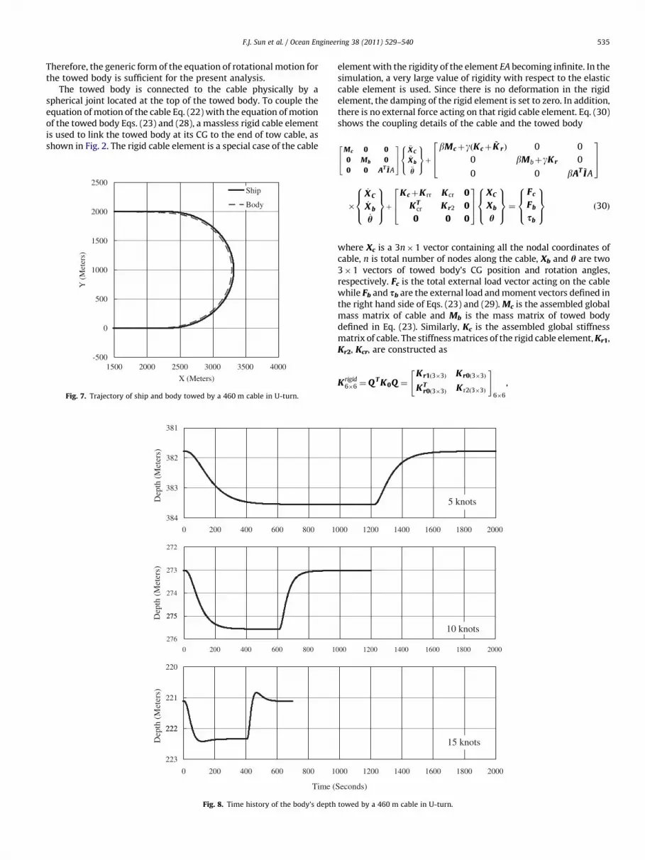
Fig. 8. Time history of the body’s depth

element with the rigidity of the element EA becoming infinite. In thesimulation, a very large value of rigidity with respect to the elasticcable element is used. Since there is no deformation in the rigidelement, the damping of the rigid element is set to zero. In addition,there is no external force acting on that rigid cable element. Eq. (30)shows the coupling details of the cable and the towed body

Mc 0 0

0 Mb 0

0 0 AT ~IA

264

375

€X C

€X b

€h

8><>:

9>=>;þ

bMcþgðKcþ~K rÞ 0 0

0 bMbþgKr 0

0 0 bAT ~IA

264

375

�

_X C

_X b

_h

8><>:

9>=>;þ

KcþKrr Kcr 0

KTcr Kr2 0

0 0 0

264

375

XC

Xb

h

8><>:

9>=>;¼

Fc

Fb

sb

8><>:

9>=>; ð30Þ

where Xc is a 3n�1 vector containing all the nodal coordinates ofcable, n is total number of nodes along the cable, Xb and h are two3�1 vectors of towed body’s CG position and rotation angles,respectively. Fc is the total external load vector acting on the cablewhile Fb and sb are the external load and moment vectors defined inthe right hand side of Eqs. (23) and (29). Mc is the assembled globalmass matrix of cable and Mb is the mass matrix of towed bodydefined in Eq. (23). Similarly, Kc is the assembled global stiffnessmatrix of cable. The stiffness matrices of the rigid cable element, Kr1,Kr2, Kcr, are constructed as

Krigid6�6 ¼Q T K0Q ¼

Kr1ð3�3Þ Kr0 3�3ð Þ

KTr0ð3�3Þ Kr2ð3�3Þ

" #6�6

,

000 1200 1400 1600 1800 2000

000 1200 1400 1600 1800 2000

000 1200 1400 1600 1800 2000

Seconds)

5 knots

10 knots

15 knots

towed by a 460 m cable in U-turn.

F.J. Sun et al. / Ocean Engineering 38 (2011) 529–540536

Krr ¼03ðn�1Þ�3ðn�1Þ 03ðn�1Þ�3

0ð3�3Þðn�1Þ Kr1ð3�3Þ

" #3n�3n

, Kcr ¼03ðn�1Þ�3

Kr0ð3�3Þ

" #3n�3

ð31Þ

The cable towed body system will be towed by either a surfaceship or a submarine at the tow point. Therefore, the boundarycondition for the Eqs. (22), (23) and (28) will be the motion ofthe tow point which is input as the prescribed positions (X, Y, Z)varying with the time. In addition, the quasi-steady state ofthe system towed in a straight line is used as initial conditions.The solution of the quasi-steady state is obtained by solving theequation of motion, Eq. (30), iteratively without the accelerationand damping terms

4. Simulation results and discussions

Based on above derivation, one would notice that the NPFEM usesthe existing finite element but changes the state variable from nodaldisplacement to nodal position. Therefore, the element used inNPFEM is the same as those used in existing FEM and we only need toexam the methodology itself. The NPFEM has been implementedinto a computer program. The equation of motion of the cable towedbody system, Eq. (30), is highly nonlinear and has been solvednumerically using the Newmark time integration scheme.

4.1. Comparison with sea trial data

Consider a submerged cable towed body system towed by asurface ship in a sea trial, see Fig. 3. The ship was travelling at a

31750

31700

31650

Ten

sion

(N

ewto

ns)

Ten

sion

(N

ewto

ns)

Ten

sion

(N

ewto

ns)

31600

32800

0 200 400 600 800

32700

32600

32500

32400

0 200 400 600 800

37000

36800

36600

36400

36200

0 200 400 600 800

Time

Fig. 9. Time history of cable (460 m) t

speed of approximately 6.17 m/s (12 knots) and executed a series ofturns. The cable was towed at 22.2 km/h (12 knots) speed while theship executed a 270-degree turn. The total cable length was 460 mwith 125 m fairing cable at the bottom and 335 m bare cable at thetop. The drag coefficients of the bare cable are

CDt ¼D0ð�0:019þ0:0239cosaþ0:02sinaþ0:001cos2aÞ

CDn ¼D0sin2a ð32Þ

while the drag coefficients of the fairing cable are

CDt ¼D0ð0:273þ0:827a2ÞcosaCDn ¼D0ð0:273þ0:827a2Þsina

9=;0orao30o

CDt ¼D0sinacosaCDn ¼D0sin2a

9=;30orar90o

9>>>>>>>>=>>>>>>>>;

ð33Þ

The bare cable was divided into nine cable elements equally whilethe fairing cable was divided into three cable elements equally. Tables 1and 2 show the parameters of the cable and towed body system.Measured ship motions at the towing point were input as theprescribed boundary conditions. Fig. 4 shows the measured shiptrajectory (thick line) together with the simulated body’s trajectory(thin line) in the horizontal plane. As the ship commences its turn, thetowed body follows the turn very closely with a slightly tighter radiusas is expected and agrees with the field observations. Along the straightsections of ship’s trajectory, the towed body is aligned with the ship’sdirection vector. The simulated time histories of the towed-body’sdepth, roll, pitch, yaw and cable tension at the towed body are then

5 knots

1000 1200 1400 1600 1800 2000

10 knots

1000 1200 1400 1600 1800 2000

15 knots

1000 1200 1400 1600 1800 2000

(Seconds)

ension at towing point in U-turn.

F.J. Sun et al. / Ocean Engineering 38 (2011) 529–540 537

compared with the measured data in Fig. 5. Good agreement isobserved between the simulation and the trial data.

4.2. Case study of a cable towed body system

4.2.1. Steady state straight tow

Steady straight tow is a typical case for the operation of thetowed cable system. In this section, we investigate the steady stateof three cable configurations (125, 293, 460 m) towed at threedifferent speeds: 9.26 km/h (5 knots), 18.52 km/h (10 knots) and27.78 km/h (15 knots), respectively. These speeds cover the mostoperational range of the towed system. Table 3 shows the threecable configurations. The first configuration is a 125 m cable, allfairing. It represents the beginning phase during deploying/reco-vering processes. The fairing cable is modeled with three elements

270.0

270.5

Dep

th (

Met

ers)

Dep

th (

Met

ers)

Dep

th (

Met

ers)

271.00 400 800

210.0

210.5

211.0

173.5

0 400 800

174.0

174.50 400 800

Time

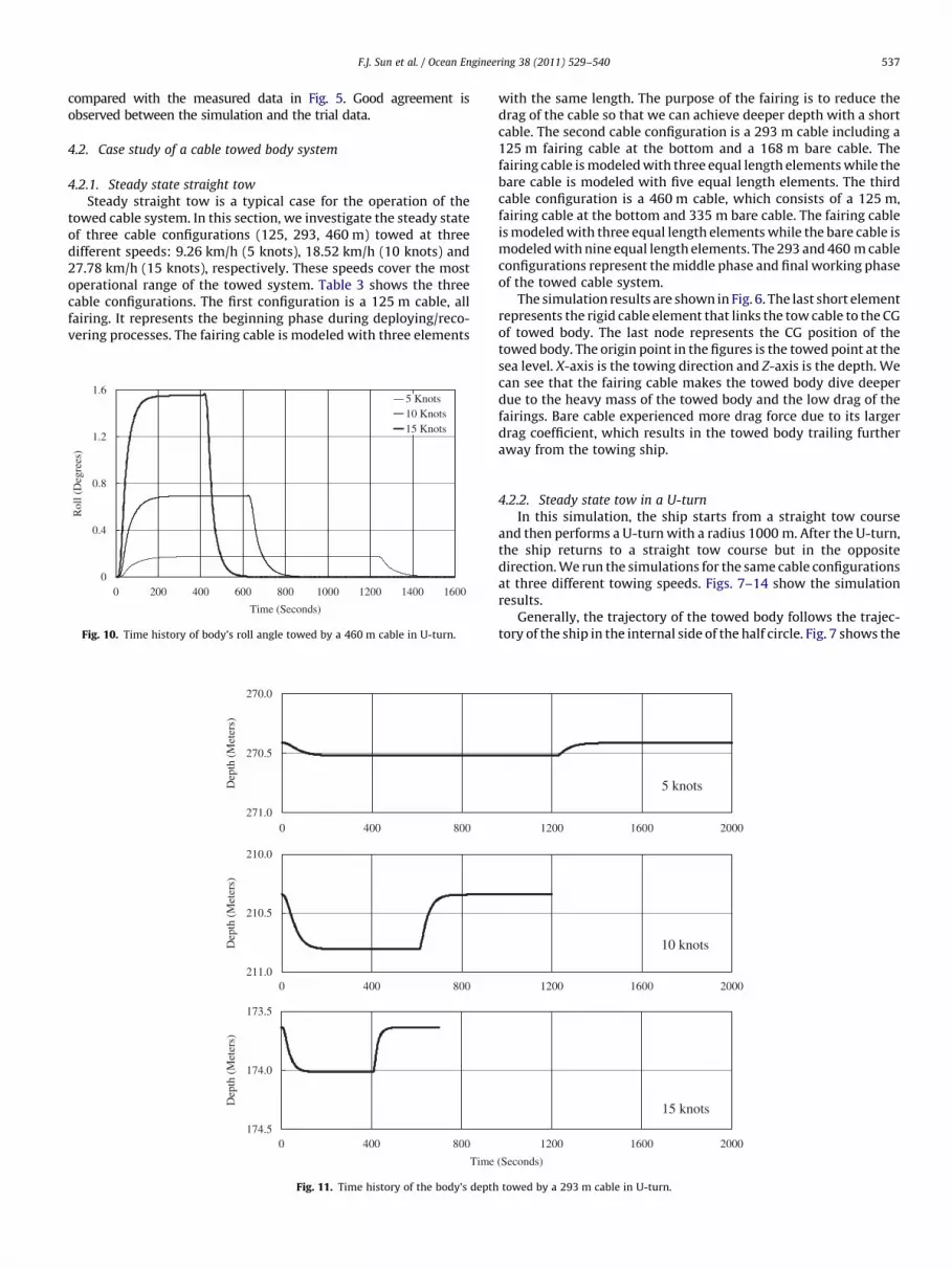
Fig. 11. Time history of the body’s depth

1.65 Knots10 Knots

1.215 Knots

0.8

Rol

l (D

egre

es)

0.4

00

Time (Seconds)

200 400 600 800 1000 1200 1400 1600

Fig. 10. Time history of body’s roll angle towed by a 460 m cable in U-turn.

with the same length. The purpose of the fairing is to reduce thedrag of the cable so that we can achieve deeper depth with a shortcable. The second cable configuration is a 293 m cable including a125 m fairing cable at the bottom and a 168 m bare cable. Thefairing cable is modeled with three equal length elements while thebare cable is modeled with five equal length elements. The thirdcable configuration is a 460 m cable, which consists of a 125 m,fairing cable at the bottom and 335 m bare cable. The fairing cableis modeled with three equal length elements while the bare cable ismodeled with nine equal length elements. The 293 and 460 m cableconfigurations represent the middle phase and final working phaseof the towed cable system.

The simulation results are shown in Fig. 6. The last short elementrepresents the rigid cable element that links the tow cable to the CGof towed body. The last node represents the CG position of thetowed body. The origin point in the figures is the towed point at thesea level. X-axis is the towing direction and Z-axis is the depth. Wecan see that the fairing cable makes the towed body dive deeperdue to the heavy mass of the towed body and the low drag of thefairings. Bare cable experienced more drag force due to its largerdrag coefficient, which results in the towed body trailing furtheraway from the towing ship.

4.2.2. Steady state tow in a U-turn

In this simulation, the ship starts from a straight tow courseand then performs a U-turn with a radius 1000 m. After the U-turn,the ship returns to a straight tow course but in the oppositedirection. We run the simulations for the same cable configurationsat three different towing speeds. Figs. 7–14 show the simulationresults.

Generally, the trajectory of the towed body follows the trajec-tory of the ship in the internal side of the half circle. Fig. 7 shows the

5 knots

1200 1600 2000

10 knots

1200 1600 2000

15 knots

1200 1600 2000

(Seconds)

towed by a 293 m cable in U-turn.

125.90

125.95

Dep

th (

Met

ers)

Dep

th (

Met

ers)

Dep

th (

Met

ers)

5 knots

126.000 400 800 1200 1600 2000

118.00

118.05

10 knots

118.10

103.80

0 400 800 1200 1600 2000

103.90

104.00

15 knots104.10

0 400 800 1200 1600 2000

Time (Seconds)

Fig. 13. Time history of body’s depth towed by a 125 m fairing cable in U-turn.

31690

5 knots31685

31680

31675

31670

32700

0 400 800 1200 1600 2000

10 knots32650

32600

32550

32500

37000

0 400 800 1200 1600 2000

15 knots36900

36800

36700

Ten

sion

(N

ewto

ns)

Ten

sion

(N

ewto

ns)

Ten

sion

(N

ewto

ns)

366000 400 800 1200 1600 2000

Time (Seconds)

Fig. 12. Time history of cable (293 m) tension at towing point in U-turn.

F.J. Sun et al. / Ocean Engineering 38 (2011) 529–540538

31678

5 knots31677

31676

31675

31674T

ensi

on (

New

tons

)T

ensi

on (

New

tons

)T

ensi

on (

New

tons

)0 400 800 1200 1600 2000

32640

3265010 knots

32630

32620

32610

32600

37000

0 400 800 1200 1600 2000

15 knots36950

36900

36850

368000 400 800 1200 1600 2000

Time (Seconds)

Fig. 14. Time history of cable (125 m) tension at towing point in U-turn.

F.J. Sun et al. / Ocean Engineering 38 (2011) 529–540 539

trajectories of the ship and the towed body for a 460 m cable at27.78 km/h (15 knots) tow speed. With other shorter cables andslower tow speeds, the radius of the towed body’s U-turn might beslightly different, but the body’s trajectories are all within the halfcircle of ship’s trajectory. When the ship enters into the turn, theforward towing speed reduces due to radial speed component. As aresult, the lift force on the towed body reduces and the towed bodydives deeper until it reaches a new balance position of circularmotion and then keeps that depth during the turn. After the shipexits the turn and moves straight again, the towed body’s depthdecreases due to the increase of towing speed in its forward axisand returns to the previous depth before the U-turn, see Fig. 8 forthe depth variations of the towed body in a U-turn towed by a460 m cable at 9.26 km/h (5 knots), 18.52 km/h (10 knots) and27.78 km/h (15 knots) tow speeds, respectively. Accordingly, as thetowed body’s depth increases, the cable tension will decrease, SeeFig. 9 for the tension variation of a 460 m cable towed at threedifferent speeds. In addition, a faster turning speed of the shipresults in larger roll angles of the towed body, see Fig. 10 for the rollangle variation in a U-turn at different tow speeds towed by 460 mcable. Similar trends can be found in simulations of 293 m cablelengths, respectively, see Figs. 11–14. However, the short cable(125 m) performs differently than the long cable. Fig. 12 shows thedepth of the towed body towed by 125 m cable actually decreasesas it enters into the curved trajectory. The reason is that the shortercable is acting like a straight bar compared to the longer cable thathas the bow-shape curved configuration, see Figs. 7 and 9. For thelong tow cable, the towed body’s trajectory is inside the curvedtrajectory of the tow ship and it moves at a slower speed than thetow ship’s speed. Thus, the towed body will dive due to the reducedlift. However, for the short tow cable, the towed body’s trajectory isactually outside the curved trajectory of the tow ship and it movesat a faster speed than the tow ship’s speed. Thus, the towed bodywill move up due to the increased lift.

5. Conclusion

A new nodal position finite element method has been developedto solve the position of the cable directly instead of the summationof displacement and previous position in the existing FEM. Theexisting FEM, which is displacement based, is prone to theaccumulated errors arising from every time step over a long timesimulation. The newly derived nodal position finite elementmethod eliminates the need of decoupling the rigid body motionfrom the total motion, where numerical errors arise in the existingnonlinear finite element method, and the limitation of smallrotation in each time step in the existing nonlinear finite elementmethod. In addition, a special element and procedure have beendeveloped to couple the cable element with the towed body.Simulation results show that this newly derived method is accurateand robust as seen in comparisons with the sea trials. Finally, casestudies of the cable towed body system are conducted for threedifferent cable configurations at three different tow speeds.

Acknowledgments

This work was supported by the National Science and Engineer-ing Research Council of Canada, Ontario Centers of Excellences andCurtiss-Wright Flow Controls, Indal Technologies.

References

Ablow, C.M., Schechter, S., 1983. Numerical simulation of undersea cable dynamics.Ocean Eng. 10 (6), 443–457.

Burgess, J.J., 1999. Equations of motion of a submerged cable with bending stiffness.J. Offshore Mech. Arct. 1-A, 283–289.

Duvat, G., Large, C., 1997. Experimental study of the dynamic behaviour of a towedsystem. In: Proceedings of the Seventh International Offshore and PolarEngineering Conference 2, pp. 17–22.

F.J. Sun et al. / Ocean Engineering 38 (2011) 529–540540

Huang, S., 1994. Dynamic analysis of three-dimensional marine cables. Ocean Eng.21 (6), 587–605.

Koh, C.G., Rong, Y., 2004. Dynamic analysis of large displacement cable motion withexperimental verification. J. Sound Vib. 272 (1–2), 187–206.

Koh, C.G., Zhang, Y., Quek, S.T., 1999. Low-tension cable dynamics: numerical andexperimental studies. J. Eng. Mech.-ASCE. 125 (3), 347–354.

Shabana, A.A., 1998. Computer implementation of the absolute nodal coordinateformulation for flexible multibody dynamics. Nonlinear Dyn. 16 (3), 293–306.

Simo, J.C., Tarnow, N., Wong, K.K., 1992. Exact energy-momentum conservingalgorithms and symplectic schemes for nonlinear dynamics. Comput. MethodsAppl. Mech. Eng. 100, 63–116.

Sun, F.J., 2010. Elastodynamic analysis of towed cable systems by a novel nodalposition finite element method, Master Thesis, York University.

Tuwankotta, J.M., Quispel, G.R.W., 2003. Geometric numerical integration applied tothe elastic pendulum at higher-order resonance. J. Comput. Appl. Math. 154 (1),229–242.

Webster, W.C., 1995. Mooring-induce damping. Ocean Eng. 22 (6), 571–591.Zhu, Z.H., Meguid, S.A., Ong, L.S., 2003, Dynamic multiscale simulation of towed

cable and body. In: Proceedings of Computational Fluid and Solid Mechanics2003, 1–2, pp. 800–803.

Zhu, Z.H., Meguid, S.A., 2006. Elastodynamic analysis of aerial refueling hose usingcurved beam. AIAA J. 44 (6), 1317–1324.

Zhu, Z.H., Morrow, B., 1998. A novel computer simulator for cable-towed submergedvehicles. Hydroelasticity Mar. Technol. (Hydroelasticity’ 98), 284–292 Fukuoka,Japan.