Dynamic model of manoeuvrability using recursive neural networks

Ocean Engineering 30 (2003) 1669–1697www.elsevier.com/locate/oceaneng

Dynamic model of manoeuvrability usingrecursive neural networks

L. Moreira∗, C. Guedes SoaresInstituto Superior Tecnico, Unit of Marine Technology and Engineering, Technical University of

Lisbon, Av. Rovisco Pais, Lisbon 1049-001, Portugal

Received 14 May 2002; received in revised form 21 August 2002; accepted 10 October 2002

Abstract

This paper presents a Recursive Neural Network (RNN) manoeuvring simulation model forsurface ships. Inputs to the simulation are the orders of rudder angle and ship’s speed andalso the recursive outputs velocities of sway and yaw. This model is used to test the capabilitiesof artificial neural networks in manoeuvring simulation of ships. Two manoeuvres are simu-lated: tactical circles and zigzags. The results between both simulations are compared in orderto analyse the accuracy of the RNN. The simulations are performed for theMariner hull. Thedata generated to train the network are obtained from a manoeuvrability model performingthe simulation of different manoeuvring tests. The RNN proved to be a robust and accuratetool for manoeuvring simulation. 2003 Elsevier Science Ltd. All rights reserved.

Keywords: Manoeuvrability; Recursive neural networks; Simulation model

1. Introduction

The Artificial Neural Networks (ANNs) have been successfully applied recentlyto a variety of problems related with naval architecture. In fact ANNs interpolationand in some cases extrapolation capability is very powerful particularly when map-ping a multi-dimensional input data space to a multi-dimensional output data spaceas demonstrated in Roskilly and Mesbahi (1996a). It is common for empirical datato be used directly for marine design and analysis. The non-linear functional mappingproperties of ANNs and their capability to learn a new set of input patterns without

∗ Corresponding author.

0029-8018/03/$ - see front matter 2003 Elsevier Science Ltd. All rights reserved.doi:10.1016/S0029-8018(02)00147-6

1670 L. Moreira, C. Guedes Soares / Ocean Engineering 30 (2003) 1669–1697

significant disturbance to the previous structure are also important factors whichmake them particularly useful for the modelling and identification of dynamic sys-tems as shown in Roskilly and Mesbahi (1996b).

For instance, simulations using ANNs have been created using data from bothmodel and full-scale submarine manoeuvres. The incomplete data measured on thefull-scale vehicle were augmented by using feedforward neural networks as virtualsensors to intelligently estimate the missing data (Hess et al., 1999). The creationof simulations at both scales permitted the exploration of scaling differences betweentwo vehicles, which is described in Faller et al. (1998).

A predictive method for the estimation of the hydrodynamic characteristics for aMariner class ship performing certain standard manoeuvres is outlined in Haddaraand Wang (1999). The method uses ANNs to predict the hydrodynamic parametersof the ship and the training data were obtained using a simulation program.

Another example of marine application of ANNs is made in catamarans or trimar-ans with unusual underwater shape, which experience great non-linearities when thevessel motions are large in magnitude. Then ANN techniques can be used to managecomplex database with a multitude of parameters and ANNs have been used to assista time-domain numerical model for prediction of pitch and heave motions of a con-cept catamaran (Atlar et al., 1997) and the UK MoD concept trimaran frigate inregular head seas (e.g. Atlar et al., 1998; Mesbahi and Atlar, 1998).

Other study concerning the identification of ship coupled heave–pitch motionsusing neural networks can be seen in Haddara and Xu (1999), where the experimentaldata were obtained using an icebreaker ship model heaving and pitching in randomwaves and it is shown that the ANNs produces good results when the system islightly damped. Still other important studies regard the reduction of roll in ships bymeans of active fins controlled by a neural network (Liut et al., 2000). Here theperformance of the fins is improved by adding an active controller. The controllercommands the rotations of the fins about a span-wise axis in order to further reducethe rolling motion. The rotations are commanded by a neural network controller. Adifferent type of application is the wind loading on ships, a model that can becomeof interest to manoeuvring problems under wind conditions (Haddara and GuedesSoares, 1999).

This brief review of the literature shows the great interest that ANN has raisedrecently in connection to applications in ship dynamics. However, the review alsoshows that the applications have been made of ANNs, which are basically staticmodels that cannot account for the changes that the system may have with time.

A Recursive Neural Network (RNN) is a computational technique for developingtime-dependent non-linear equation systems that relate input control variables to out-put state variables. A recursive network is one that employs feedback; namely, theinformation stream issuing from the outputs is redirected to form additional inputsto the network. For this application, the RNNs are used to predict the time historiesof the manoeuvring variables velocities of sway and yaw.

The objective of the new predictive tool is an alternative to the usual manoeuvringsimulators that use traditional mathematical models, which are function of the hydro-dynamic forces and moment derivatives. These values are normally achieved from

1671L. Moreira, C. Guedes Soares / Ocean Engineering 30 (2003) 1669–1697

experiments performed with models in tanks. This procedure is time consuming andcostly, requiring exclusive use of a large specialised purpose built facility. Anotherdisadvantage of this method is the intrinsic scale effect model-real ship. Anyway,this is the unique valid method that can be used in the design stage of a ship.

The alternative RNN model presented in this paper represents an implicit math-ematical model for ships, which time histories of manoeuvring motions are pre-viously known. The input of this model will be just the time histories of the motionsof sway and yaw and also the required advance speed of the ship and respectiverudder angle. The main advantage of this method consists in that these parametersare easily obtained from full-scale trials of ships existing, making this procedureeasier to perform and less expensive.

This paper shows the results of the comparison between simulations with a math-ematical model and the simulations made with the RNN model after the training ofdata obtained through the first simulator. The purpose of this is to validate the modeland to show that it is an accurate predictive tool and is able to fit the results achievedwith other formulation.

The simulation data describing a series of manoeuvres with varying rudder deflec-tion angles and approach speeds have been acquired for the Mariner ship hull (Craneet al., 1989) and these data have been used to train and validate two neural networks,one for each type of manoeuvre: tactical circles or zigzags.

2. Description of the ship mathematical model

It is assumed that the planar motion of the ship is not affected by the ship’s roll;this assumption makes it possible to eliminate the roll equation. On this model willnot be inserted the equations referred to the propeller thrust and torque equations.Therefore, this model will be easily connected to the propulsion simulation modeldescribed in Moreira et al. (2000). Also, symmetry in relation to midship plane isconsidered here, which is typical for ships with just one shaft line. A first-orderdifferential equation is considered to describe the steering gear dynamics.

The orthogonal coordinates system (Euler coordinates) is the most widely used.The standard body axis Gxy have the origin in the centre of mass of the ship G, thex-axis is directed forward and the y-axis to the starboard. At certain instant t theseaxes will coincide with the inertia axis Oxh. The instantaneous position of the shipis described by the coordinates of the centre of mass x and h, as well as by theheading angle between the axis x and x with the positive direction being clockwise.The motion of the ship is decomposed in surge velocity u, sway velocity v and yawangular velocity r (positive clockwise). The speed of the ship can be given in thefollowing form: V = (u2 + v2)1/2. The hydrodynamic forces that act in the hull resultin a surge force X, a sway force Y and a yaw moment N. The rudder angle dR isassumed to be positive when is directed to starboard.

The frames and kinematical parameters that are standard in ship manoeuvrabilityare shown in Fig. 1. The drift angle b is not required to appear in the mathematicalmodel but will be calculated to allow the observation of its behaviour along the time.It is defined as being equal to

1672 L. Moreira, C. Guedes Soares / Ocean Engineering 30 (2003) 1669–1697

Fig. 1. Frames of reference and main parameters.

b � �arcsin(v /V) (1)

and is positive for the right side.The equation of dynamics can be written in its standard form as following:

X � m(u�vr) Y � m(v � ur) N � Izzr (2)

where the dots mean the derivatives with respect to time, m the ship’s mass, and Izz

is the moment of inertia of the ship in relation to the centre of mass.The mass can be represented by

m �r2

m�L2T (3)

where m� is the non-dimensional mass, L the length of the ship and T is the draughtof the ship. The gyration radius is assumed to be equal to L/4 (value usually assumed)and the moment of inertia can be estimated as being equal to

Izz � 0.0625mL2 (4)

And the main characteristics of the Mariner ship (Crane et al., 1989) are

L � 100 m

B � 15 m

T � 5 m

The kinematical equations are

x � u cosy�v siny h � u siny � v cosy j � r (5)

The governing equation is

1673L. Moreira, C. Guedes Soares / Ocean Engineering 30 (2003) 1669–1697

dR �1

TR(d∗�dR) (6)

where TR is the steering gear time lag (it is assumed as being equal to 5 s) and d∗

is the rudder order requested.Simultaneously, the following inequalities must be respected:

�dR��dm (7)

�d∗��dm (8)

�dR��em (9)

where dm is the maximum rudder angle and �m is the maximum deviation rate. The

standard values are 35° for dm and 213° / s for �m.

Initially, it is required to unify the hydrodynamic forces of surge and sway with theacceleration-independent-inertial terms and to consider the acceleration-dependent-inertial hydrodynamic forces through the added masses m11 and m22. Thus, thedynamic equations can be rewritten as follows:

X � (m � m11)u Y � (m � m22)v N � (Izz � m66)r (10)

where X = mvr + X+m11u; Y = �mur + Y+m22v, and N = N+m66r.The modified surge force X at u�0 can be represented as follows:

X � (m � Cmm22)vr � TE(u,n) � CRu2 �r2

LTX�ddu2d2R (11)

where Cm is the Inoue coefficient (Crane et al., 1989) TE the effective thrust, CR theresistance factor, and X�dd is the dimensionless hydrodynamic derivative.

The CR factor is dimensional and can be expressed through the dimensionless dragcoefficient CTL as follows (Van Mannen and Van Oossanen, 1989):

CR �mL

CTL (12)

The modified sway force Y is given by

Y � �mur �r2

LTV2Y� (13)

where Y� is the sway force coefficient and the yaw moment is given by

N �r2

L2TV2N� (14)

with N� representing the yaw moment coefficient.The mathematical models for the sway force and yaw moment coefficients include

the numerical values for the hydrodynamic derivatives and other constant parametersrelated with the forces components that act in the hull and rudder.

1674 L. Moreira, C. Guedes Soares / Ocean Engineering 30 (2003) 1669–1697

The sway force and yaw moment coefficients are described by conventional poly-nomial regression models

Y� � Y�vv� � Y�rr� � Y�vvvv�3 � Y�vvrv�2r� � Y�ddR � Y�vvdv�2dR N� (15)

� N�vv� � N�rr� � N�vvvv�3 � N�vvrv�2r� � N�ddR � N�vvdv�2dR

where Y�v, …, N�vvd are hydrodynamic derivatives and v� and r� are non-dimensionalkinematical parameters usually defined as being equal to:

v� � v /V r� � rL /V (16)

In order to make the ship mathematical model more flexible it was assumed thatthe linear hydrodynamic derivatives are dependent of the trim and the well-knownformulas of Inoue (Crane et al., 1989) were used to take this fact into account:

Y�v � (1 � b1d)Y�v0 Y�r � (1 � b2d)Y�r0 N�v � (1 � b3d)N�v0 N�r (17)

� (1 � b4d)N�r0

where d = d /T is the relative trim; the absolute trim d is positive by stern and thesubscript 0 is referred to null trim values. The parameters b1, …, b4 are

b1 � 0.6667 b2 � 0.8 b3 � �0.27Y�v0 /N�v0 b4 � 0.3 (18)

The method of accounting for trim was derived from other mathematical model offorces applied in the hull, but through the comparison with other estimation methodof Fedyaevsky and Sobolev (1964) and with basis on the slender body theory it wasdemonstrated that the first method is of a general nature and that can be applied toany mathematical model in order to obtain realistic estimations.

Considering the original polynomial expressions presented in Crane et al. (1989),the regressors v�d2

R, d3R must be eliminated from the polynomial regression models

(15) as well as the constant terms that take into account with the asymmetry inrelation to the centre-plane because estimating their influence they show to be of norelevant importance.

The numerical values of the hydrodynamic derivatives Y�v, …, N�vvd, the non-dimensional added masses k11 = m11 /m, k22 = m22 /m and k66 = m11 / Izz and otherconstant parameters are given in Table 1.

The mathematical model of the ship is obviously non-linear. Therefore, a linearsystem was chosen to start implementing to observe how it behaves. This meansthat the non-linear basic model has to be linearised, it is necessary to synthesise acontroller for the linearised system and then to test its applicability to the originalnon-linear dynamic system.

The usual method of linearisation implicates the removal of all non-linear termsof the dynamic equations of motion. The resulting linearised mathematical model isvalid but just in the absence of disturbances to the motion because in the coursechanging manoeuvres, in general, variations in the kinematical parameters of nonegligible value exist. In principle, it is possible to conclude the linearisation in theneighbourhood of any current values of state variables but this, firstly, will lead tounstable linearised mathematical models in some cases and secondly will be an over-

1675L. Moreira, C. Guedes Soares / Ocean Engineering 30 (2003) 1669–1697

Table 1Values of the dimensionless parameters that define the hydrodynamic forces of the Mariner ship

Parameter Symbol Value

Relative added masses K11 0.03K22 0.9K66 0.63

Drag coefficient CTL 0.07Inoue’s coefficient Cm 0.625Hydrodynamic derivatives X�dd �0.02

Y�v �0.244Y�r 0.067Y�vvv �1.702Y�vvr 3.23Y�d �0.0586Y�vvd �0.25N�v �0.0555N�r �0.0349N�vvv 0.345N�vvr �1.158N�d 0.0293N�vvd �0.1032

load of additional calculations as explained in Sutulo (1997) and Sutulo et al. (2002).On this case, it was decided to linearise the original non-linear mathematical modelby the least mean square method in a reasonable finite domain in state-space. Thisapproach has the advantage of being used just once in the initialisation state, andits most important benefit is the ability to obtain a stable linearised mathematicalmethod even in the case of directionally unstable ships.

It is assumed that the surge motion has little influence in the transversal motion(sway + yaw). This makes it possible to linearise just of the sway and yaw equationswhere the surge velocity u�V. When using linearised mathematical models, it ismore convenient to operate them in the dimensionless form. The kinematic para-meters v� and r� were already introduced and now will appear the non-dimensionalstandard time t� that is defined as dt� = dt(V /L). Then, the sway and yaw equationsappear as

m’22v’ � fY(v’ ,r’ ,dR) m’

66r’ � fN(v’ ,r’ ,dR) (19)

where the dots above the symbols mean the derivative with respect to non-dimen-sional time; the non-dimensional coefficients of inertia are

m�22 �2(m � m22)rL2T

m�66 �2(Izz � m66)rL4T

(20)

and the second member of the equations

fN(v�,r�,dR) � N�vv� � N�rr� � N�vvvv�3 � N�vvrv�2r� � N�ddR

1676 L. Moreira, C. Guedes Soares / Ocean Engineering 30 (2003) 1669–1697

� Y�vvdv�2dRfY(v�,r�,dR) � Y�vv� � (Y�r�m�)r� � Y�vvvv�3 � Y�vvrv�2r� (21)

� Y�ddR � Y�vvdv�2dR

where the non-dimensional mass of the ship is given by

m� �2mrL2T

(22)

A set of linear equations will be considered instead of non-linear Eqs. (19)

m�22v� � CvYv� � Cr

Yr� � CdYdR m�66r� � CvNv� � Cr

Nr� � CdNdR (23)

where the linearised hydrodynamic derivatives CvY, ..., CdN in the second members of

the equations are determined by the least square principle:

(CvY,Cr

Y,CdY) � arg min�r�L

�r�L

�v’L

�v�L

�dL�dL

[fY(v�,r�,dR)�(CvYv� � Cr

Yr�

� CdYdR)]2 dr� dv� ddR (CvN,Cr

N,CdN) � arg min�r�L

�r�L

�v�L

�v�L

�dL�dL

[fN(v�,r�,dR) (24)

�(CvNv� � Cr

Nr� � CdNdR)]2 dr� dv� ddR

where v�L, r�L and dL are parameters that define the dimensions and area of thelinearisation domain. They are correlated with the expected variations of the kinem-atic parameters but in fact their values might be empirically set in order to obtainthe most consistent linearised model.

Eq. (24) lead to the following sets of normal equations (similar for both Y andN components):

�r�L

�r�L

�v�L

�v�L

�dL�dL

[fY,N(v�,r�,dR)�(CvY,Nv� � Cr

Y,Nr� � CdY,NdR)]v� dr� dv� ddR � 0

�r�L

�r�L

�v�L

�v�L

�dL�dL

[fY,N(v’ ,r’ ,dR)�(CvY,Nv� � Cr

Y,Nr� � CdY,NdR)]r� dr� dv� ddR � 0 (25)

�r�L

�r�L

�v�L

�v�L

�dL�dL

[fY,N(v�,r�,dR)�(CvY,Nv� � Cr

Y,Nr� � CdY,NdR)]dR dr� dv� ddR � 0

For this particular non-linear regression model for sway force and yaw momentcoefficients the triple integrals are easily calculated explicitly and the resulting equa-tions for the linearised hydrodynamic derivatives appear simply in the followingform:

CvY � Y�v �

35

Y�vvvv�2L Cr

Y � Y�r�m� �13Y�vvrv�2

L CdY � Y�d �13

Y�vvdv�2L Cv

N (26)

� N�v �35

N�vvvv�2L Cr

N � N�r �13N�vvrv�2

L CdN � N�d �13

N�vvdv�2L

1677L. Moreira, C. Guedes Soares / Ocean Engineering 30 (2003) 1669–1697

The resulting formulation does not contain r�L and dL. It is obvious that when v�L

tends to zero, the linearised generalised hydrodynamic derivatives become similar tothe linear derivatives in the polynomial expansion. This means that the linearisationtechnique follows the usual linearisation (differential) and its particular case corre-sponds to the linearisation in the infinitesimal domain.

It is more convenient to rewrite the linearised Eqs. (23) for further transformationsin the following way:

m�22v� � CvYv� � Cr

Yr� � CdYdR m�66r� � CvNv� � Cr

Nr� � CdNdR (27)

where

CvY � �Cv

Y, CrY � �Cr

Y, CvN � �Cv

N, CrN � �Cr

N (28)

The set of Eqs. (27) can be transformed in the yaw equivalent second-order Nom-oto equation:

T�1T�2r� � (T�1 � T�2)r� � r� � K�(dR � T�3dR) (29)

which can be approximated by the first-order Nomoto equation:

T�r� � r� � K�dR (30)

The non-dimensional time lags T�1, T�2, T�3 and T�, as well as the gain of the shipK� are related with the previously defined parameters of set (28) through the follow-ing equalities:

T�1 � �1p1

, T�2 � �2p2

, T�3 � �EF

, T� � T�1 � T�2�T�3, K� �FC

p1

� �BA

�p2, p2 ��B��B2�4AC

2AA � m�22m�66, B � m�22Cr

N (31)

� m�66CvY, C � Cv

YCrN�Cv

NCrY, E � m�22CdN, F � Cv

YCdN�CvNCdY

where p1 and p2 are, obviously, the poles of the linearised model and the remaindervariables are of auxiliary character.

3. Structure of the simulation model

The learning problem through neural networks described here will consist of simu-lating the velocities of sway, v(t), and yaw, r(t), assuming that input parameters arethe rudder angle, d(t), and the ship’s speed, V(t). The neural network inputs will bethe rudder angle, d(t), and the ship’s speed, V(t) and also the velocities of sway,v(t�1), and yaw, r(t�1). All these data will be obtained from manoeuvrability simul-ations with the manoeuvrability model implemented in a block diagram in Simulink.

1678 L. Moreira, C. Guedes Soares / Ocean Engineering 30 (2003) 1669–1697

The network outputs will be the velocities of sway, v(t), and yaw, r(t).The kinematical equations used for the trajectories calculation are the ones referred

in Eqs. (5). The RNN will be trained to imitate the parameters of sway and yawresulting from the simulations for different speeds and rudder angles requested.

Fig. 2 illustrates the representation used in this version of the RNN simulator andshows the type of typical representation of many systems of ANNs. Each node(circle) in the network diagram corresponds to the output of a unit and the lines thatinput the node from left are its inputs. As can be seen, there are 10 units that receiveinputs directly from the achieved data. These units are called ‘hidden’ units becausetheir output is valid just inside the network and are not valid as part of the globalnetwork output. Each one of these 10 hidden units computes a single real outputbased on a weighted combination of their inputs. These outputs of the hidden unitsare then used as inputs of a second layer of two output units. Each output correspondsto either a velocity of sway or yaw in the instant t and these outputs will again inputthe network (cyclic) as being the inputs sway and yaw in the instant t�1.

This network structure is typical of many ANNs. Here the individual units areinterconnected in layers. In general, ANNs can have with many other types of struc-tures—acyclics or cyclics, directs or indirects. In this paper will be used the approxi-mation with ANNs more common and practical, which is based in the Backpropag-ation algorithm.

The simplified mathematical model described in Section 2 was implemented usingthe software MatLab and its toolbox Simulink. This software was chosen due toits interface capability with the user and due to the easy visualisation and comprehen-sion of the system. The Simulink has several algorithms to solve differential equa-tions, and for this particular case was chosen the Runge–Kutta method. The completeblock diagram of the model is illustrated in Fig. 3. Although this model is a variationof a more complex model that allows obtaining the ship’s trajectory with good accu-racy (e.g. Sutulo, 1997; Sutulo et al., 2002), this has the advantage to allow a rapidvisualisation of the manoeuvres because it allows a reasonable interface with the user.

Fig. 2. RNN to simulate ship’s manoeuvrability.

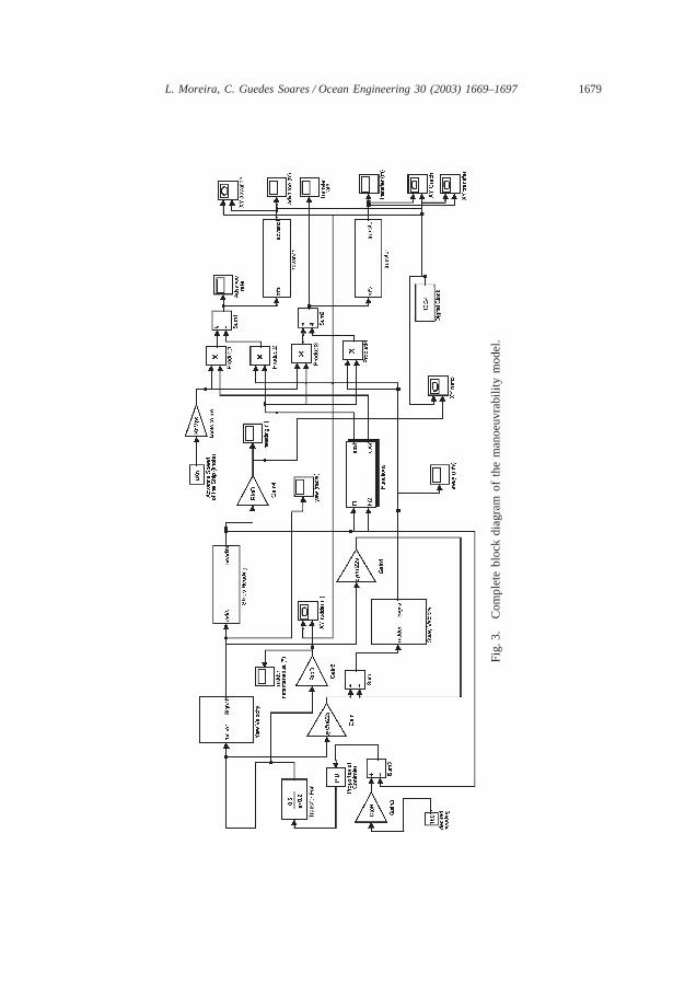
1679L. Moreira, C. Guedes Soares / Ocean Engineering 30 (2003) 1669–1697

Fig.

3.C

ompl

ete

bloc

kdi

agra

mof

the

man

oeuv

rabi

lity

mod

el.

1680 L. Moreira, C. Guedes Soares / Ocean Engineering 30 (2003) 1669–1697

4. Validation of the learning through ANNs to the case study

ANN training methods are adequate even for those problems where the trainingdata correspond to noisy data, as can be the case of the data achieved on board infull-scale manoeuvring trials.

One of the potential capabilities of the model described in this paper will be thesimulation of the motions using training data obtained from full-scale tests. Workin this field has been developed and an improved RNN manoeuvring simulation toolfor surface ships, trained and validated with data acquired from two ships operatingin the open ocean, is described in Hess and Faller (2000).

The Backpropagation algorithm is the most widely used learning technique forANNs. It can be used in problems with the following characteristics:

� The training examples can contain errors. The learning methods through ANNsare quite robust to noise in the training data.

� Long training timings are acceptable. Typically the network training algorithmsrequire long training timings. The training timing can vary between some secondsand many hours, depending of factors such as the number of weights in the net-work, the number of considered training examples and the assumed values forthe learning algorithm parameters.

� A quick evaluation of the target (desired) function learned can be required.Although the training timings of the ANN can be long, the evaluation of thelearned network, in such a way to apply it to a subsequent example, is typicallyvery fast.

� The ability of human understanding the learned target function is not important.The learned weights through neural networks are usually hard to interpret byhuman.

5. Network elements

Data for training, cross-validation and testing the neural networks were acquiredfrom simulations performed with the manoeuvrability model implemented in a blockdiagram. Because the manoeuvring simulations exhibit similar turning characteristicsfor both right and left turns, the simulation performed were just for positive rud-der angles.

The architecture of the neural network is illustrated schematically in Fig. 4. Thenetwork consists of three layers: an input layer, one hidden layer and an output layer.Within each layer are nodes, which contain a non-linear transfer function that oper-ates on the inputs to the node and produces a smoothly varying output.

The binary sigmoid function was used for this work; for an input x it producesthe output y, which varies from 0 to 1 and is defined by

y(x) �1

1 � e�x (32)

1681L. Moreira, C. Guedes Soares / Ocean Engineering 30 (2003) 1669–1697

Fig. 4. Recursive neural network.

Note that the nodes in the input layer simply serve as a means to couple the inputsto the network; no computations are performed within these nodes. The nodes ineach layer are fully connected to those in the next layer by weighted links. As datatravel along a link to a node in the next layer and are multiplied by the weightassociated with that link.

The weighted data on all links terminating at a given node are then summed andforms the input to the transfer function within that node. The output of the transferfunction then travels along multiple links to all the nodes in the next layer, and soon. So, as shown in Fig. 4, an input vector at a given time step travels from left toright through the network where it is operated on many times before it finally pro-duces an output vector on the output side of the network. Not shown in Fig. 4 isthe fact that most nodes have a bias; this is implemented in the form of an extraweighted link to the node. The input to the bias link is the constant 1, which ismultiplied by the weight associated with the link and then summed along with theother inputs to the node.

An RNN has feedback; the output vector is used as additional inputs to the networkat the next time step. For the first time step, when no outputs are available, theseinputs are filled with initial conditions. The network described here has four inputs.The hidden layer contains 10 nodes and each of these nodes uses a bias. The outputlayer consists of two nodes, and also uses bias units. The network contains 16 compu-tational nodes and a total of 72 weights and biases. The input vector consists of therudder angle and advance speed of the ship, and the network then predicts at eachtime step the sway velocity component v and the yaw velocity component r. Thesevelocity predictions are then used to compute at each time step the heading angle

1682 L. Moreira, C. Guedes Soares / Ocean Engineering 30 (2003) 1669–1697

and the trajectory components. Recursed outputs from the prior step are used as twoadditional contributions to the input vector. The collection of input and correspondingtarget output vectors comprise a training set, and these data are required to preparethe network for further use. Data files containing time histories of tactical circlesand zigzag manoeuvres formed the training sets.

After the neural network has been successfully trained using cross-validation, theweights that provide the minimum error to the network are saved. Thus, the networkmay be presented with an input vector similar to the input vectors in the trainingset (i.e. drawn from the same parameter space), and it will then produce a predictedoutput vector. This ability to generalise, i.e. to produce reasonable outputs for inputsnot encountered in training is what allows neural networks to be used as simulationtools. To test the ability of the network to generalise, a separated subset of test datafiles must be used. These test data files then demonstrate the predictive capabilitiesof the network.

Two neural networks were trained in this manner to predict tactical circles andzigzags. In each case about 70% of the data files comprised the training set with30% set aside as cross-validation files. The networks were trained for 65,500 iter-ations (epochs). In each iteration, the time series are presented for all inputs andoutputs for all files in the training set. During this training process, training is pausedevery 10 iterations, and the network is tested for its ability to generalise. To carrythis out, all of the files in the training set are combined with the cross-validationfiles and the entire set is presented to the network.

After training has concluded, one examines the error measures as a function ofthe number of iterations at which training should have ceased and where minimumabsolute errors and maximums in the measures occur. The best performance for thetactical circle network was achieved at epoch 23,003 for the cross-validation set andat epoch 65,500 for the training set and the best performance for the zigzag networkwas achieved at epoch 65,500 for both cross-validation and training sets.

Summarising, two neural networks were trained to predict tactical circles and zig-zags using the procedure described in this section. The results of these simulationsare detailed in Section 6.

The non-linear activation function used in this case is the sigmoid function thathas saturation values of (0.1). Presenting a data set whose values are not boundedby the saturation range will force the neurone to its saturation point and it will nolonger respond to changes in input. In this case study was chosen to normalise thedata between 0.2 and 0.8.

6. Case study: simulation of the manoeuvrability characteristics of ships

In the following case study, the results achieved using RNNs and conventionalmathematical models built in a form of block diagram are compared.

The learning objective in this case evolves the classification of the sway and yawvelocities of the ship to several rudder angles and advance speed. Sampling periodused was 1 s and 22 runs of simulated data are available, i.e. 16 tactical circles andsix zigzags.

1683L. Moreira, C. Guedes Soares / Ocean Engineering 30 (2003) 1669–1697

Table 2Range of variation of the tactical circle network parameters

Variable Min Max

d (deg) 0 35V (knots) 3.7 15v (m/s) 0 0.99r (rad/s) �0.023 0

Two target functions will be trained through the data obtained in the manoeuvr-ability simulations. Given as input the rudder angle, the advance speed of the ship,sway and yaw at the instant t�1, the RNN can be trained to produce as outputs thesway and yaw velocities at the instant t.

6.1. Modelling options

6.1.1. Input encodingGiven that the input of the RNN will be a representation of the order of manoeuvr-

ing of the ship, a modelling key is how to encode this order. One option could bejust to use the rudder angle and the advance speed of the ship as inputs. One difficultythat could happen with this option would be that this leads to a higher variablenumber of manoeuvring characteristics (velocities of sway and yaw) for each instantof manoeuvre. Taking as inputs the rudder angle, the advance speed of the ship andalso the velocities of sway and yaw at the instant t�1 the possible number of vari-ables will be decreased in the learning of the velocities of sway and yaw at theinstant t. Table 2 shows the ranges of variation of the parameter’s values evolvedin the tactical circles network.

Table 3 shows the ranges of variation of the parameter’s values evolved in thezigzags network. All these values were normalised between 0.2 and 0.8 in order thatthe inputs of the network have values in the same range that the activation of thehidden unit and output unit.

Table 3Range of variation of the zigzags network parameters

Variable Min Max

d (deg) �20 20V (knots) 4.5 15v (m/s) �0.56 0.56r (rad/s) �0.013 0.013

1684 L. Moreira, C. Guedes Soares / Ocean Engineering 30 (2003) 1669–1697

Table 4Tactical circles-simulation runs executed for training, cross-validation and test

No. Test Approach speed Rudder angle (deg)(knots)

1 Circle Max Max2 Circle 75% Max Max3 Circle 50% Max Max4 Circle 25% Max Max5 Circle Max 75% Max6 Circle 75% Max 75% Max7 Circle 50% Max 75% Max8 Circle 25% Max 75% Max9 Circle Max 50% Max10 Circle 75% Max 50% Max11 Circle 50% Max 50% Max12 Circlea 25% Max 50% Max13 Circlea Max 25% Max14 Circlea 75% Max 25% Max15 Circlea 50% Max 25% Max16 Circlea 25% Max 25% Max17 Circleb 70% Max Max18 Circleb 60% Max Max19 Circleb 30% Max 50% Max20 Circleb Max 35% Max21 Circleb 95% Max 30% Max22 Circleb 40% Max 25% Max

a Circles used for cross-validation.b Circles used for test.

Fig. 5. Test 6: Time histories for sway and yaw—75% max rudder angle; 75% max speed.

1685L. Moreira, C. Guedes Soares / Ocean Engineering 30 (2003) 1669–1697

Fig. 6. Test 6: Ship’s trajectory—75% max rudder angle; 75% max speed.

Fig. 7. Test 9: Time histories for sway and yaw—50% max rudder angle; max speed.

6.1.2. Output encodingThe RNN must provide as output values the sway and yaw velocities for each

instant t. The output values were also normalised between 0.2 and 0.8. If one triesto train the network to tune the desired values exactly equal to 0 and 1, the gradientdescent will force the weights to grow without limit. On the other hand, the values0.2 and 0.8 are obtained using a sigmoid unit with finite weights.

6.1.3. Network structureFor this work a standard structure of an RNN, using two layers of sigmoid units

(one hidden layer and one output layer), was selected. Using 16 manoeuvres, thetraining time was approximately 3 h and 10 min using a Pentium III (450 MHz) forthe tactical circles network. For the zigzag network we used six manoeuvres and thetraining time was approximately 1 h and 20 min using the same processor.

1686 L. Moreira, C. Guedes Soares / Ocean Engineering 30 (2003) 1669–1697

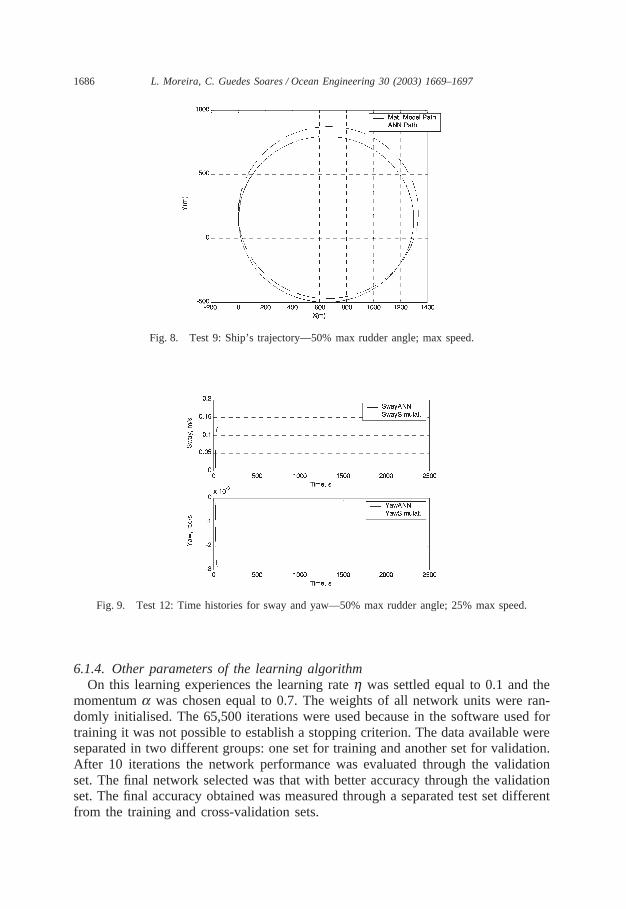
Fig. 8. Test 9: Ship’s trajectory—50% max rudder angle; max speed.

Fig. 9. Test 12: Time histories for sway and yaw—50% max rudder angle; 25% max speed.

6.1.4. Other parameters of the learning algorithmOn this learning experiences the learning rate h was settled equal to 0.1 and the

momentum a was chosen equal to 0.7. The weights of all network units were ran-domly initialised. The 65,500 iterations were used because in the software used fortraining it was not possible to establish a stopping criterion. The data available wereseparated in two different groups: one set for training and another set for validation.After 10 iterations the network performance was evaluated through the validationset. The final network selected was that with better accuracy through the validationset. The final accuracy obtained was measured through a separated test set differentfrom the training and cross-validation sets.

1687L. Moreira, C. Guedes Soares / Ocean Engineering 30 (2003) 1669–1697

Fig. 10. Test 12: Ship’s trajectory—50% max rudder angle; 25% max speed.

Fig. 11. Test 17: Time histories for sway and yaw—max rudder angle; 70% max speed.

6.2. Results

Beginning with the RNN to simulate the tactical circles, the network was trainedusing 11 tactical circles with five set aside for cross-validation. A set of six tacticalcircles was also used for test. All these manoeuvres are described in Table 4. Figs.5–16 depict the time histories for sway and yaw and the circle trajectories obtainedthrough the RNN simulation superimposed upon the time histories and the circletrajectories obtained through the simulation with the previous model. In each casethe only information provided to the trained network were the time histories for therudder deflection angle and for the advance speed of the ship and the initial con-ditions of the vehicle. The training runs that are shown are comprised by two of the11 manoeuvres used for training, one of the five validation runs and three separatedcircles used for test. The two training runs that are shown represent a mixture of

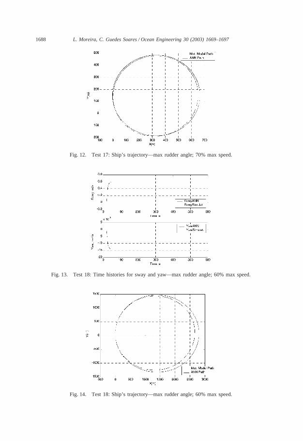
1688 L. Moreira, C. Guedes Soares / Ocean Engineering 30 (2003) 1669–1697

Fig. 12. Test 17: Ship’s trajectory—max rudder angle; 70% max speed.

Fig. 13. Test 18: Time histories for sway and yaw—max rudder angle; 60% max speed.

Fig. 14. Test 18: Ship’s trajectory—max rudder angle; 60% max speed.

1689L. Moreira, C. Guedes Soares / Ocean Engineering 30 (2003) 1669–1697

Fig. 15. Test 20: Time histories for sway and yaw—35% max rudder angle; max speed.

Fig. 16. Test 20: Ship’s trajectory—35% max rudder angle; max speed.

two different rudder angles and two different approach speeds. The test manoeuvrescomprise a mixture of two different rudder angles with three different approachspeeds. Solid lines represent the simulation using the RNN and the dashed lines areused for the previous predictions. In all the cases the circles are simulated with inputfor the rudder angle a step function at 20 s.

The predictions for the training circles are quite good. The trained network haslearned how to perform a tactical circle manoeuvre. This is evident by the perform-ance of the network on the test circles. Recall that the test runs were never used tomodify the weights during training, and in this sense, have never been used bythe network.

The RNN has been successfully able to generalise, i.e. to make predictions formanoeuvres different from, but similar to those represented in the training set. To

1690 L. Moreira, C. Guedes Soares / Ocean Engineering 30 (2003) 1669–1697

Table 5Tactical circles error measures averaged over all manoeuvres/averaged over test runs only

Variable Absolute error %

v 0.0182/0.0171 m/s 4.9/4.6r 0.00042/0.00041 rad/s 4.8/4.7x 90/86 m 5.7/5.5y 90/86 m 5.7/5.5

quantify the convergence of the RNN, averaged errors of the tactical circles havebeen tallied in Table 5 for the four critical variables: v, r, x and y.

Figs. 17 and 18 depict the errors for a set of training and cross-validation dataruns for complete and steady manoeuvres, respectively. Figs. 19 and 20 show theerrors for the set of test manoeuvres. In Table 5 the first number in each cell is anerror averaged over all 22 manoeuvres, whereas the second number is the erroraveraged over the six test circles only. To give some percentage errors, the absoluteerrors were normalised by the following scales: average sway velocity in the turn0.375 m/s, average yaw velocity in the turn of 0.00876 rad/s and an average turningdiameter of 1577 m.

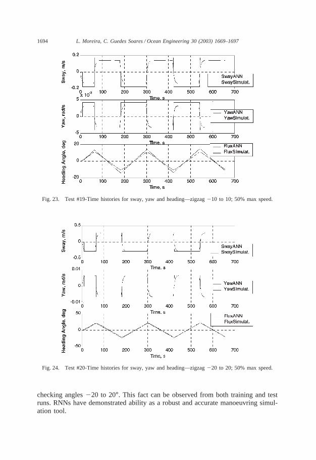
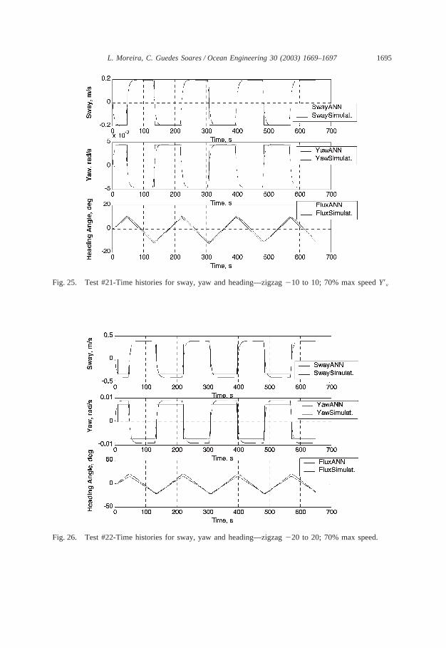
The zigzag RNN was trained using three zigzags with one set aside for cross-validation. A set of two zigzags was also used for test. All these manoeuvres aredescribed in Table 6. Figs. 21–26 depict the predicted time histories for sway, yawand heading using the RNN and the previous model. The four training runs that areshown represent a mixture of two different rudder checking angles and two differentapproach speeds. The test manoeuvres comprise two different rudder checking anglesand one approach speed.

Fig. 17. Comparison between methods for complete manouvers—training and cross-validation data runs.

1691L. Moreira, C. Guedes Soares / Ocean Engineering 30 (2003) 1669–1697

Fig. 18. Comparison between methods for steady manouver—training and cross-validation data runs.

Fig. 19. Comparison between methods for complete manouvers—test data runs.

The zigzag manoeuvre is a more complex manoeuvre than the tactical circle andyet the network trained satisfactory well to the data. The results for the zigzagsnetwork are shown in Table 7 for the three critical variables: v, r and y. The firstnumber in each cell is an error averaged over all eight manoeuvres, whereas thesecond number is the error averaged over the two test runs only. The percentageerrors were obtained by normalising with: average steady sway velocity in themanoeuvre of 0.3086 m/s, average steady yaw velocity in the manoeuvre of 0.00718rad/s and an average peak-to-peak heading variation of 32°.

To make some estimates of precision error manoeuvres with the same rudder

1692 L. Moreira, C. Guedes Soares / Ocean Engineering 30 (2003) 1669–1697

Fig. 20. Comparison between methods for steady manouver—test data runs.

Table 6Zigzags-simulation runs executed for training, cross-validation and test

# Test Approach speed (knots) Rudder angle (deg)

17 Zigzag Max �10 to 1018 Zigzag Max �20 to 2019 Zigzag 50% Max �10 to 1020 Zigzaga 50% Max �20 to 2021 Zigzagb 70% Max �10 to 1022 Zigzagb 70% Max �20 to 20

a Zigzags used for cross-validation.b Zigzags used for test.

deflection and approach speeds were compared. For the tactical circles, the steadysway velocity in the turn varied by 0.0025–0.0624 m/s or 2–10.5%, the steady yawvelocity in the turn by 0.0000724–0.0015 rad/s or 3–10.8% and the turning diameterdiffered by 6–220 m or 1–8%. For the zigzags the steady sway velocity in themanoeuvre varied by 0.0026–0.23 m/s or 1–41%, the steady yaw velocity in themanoeuvre varied by 0.000053–0.0055 rad/s or 0.8–42% and the peak-to-peak head-ing differed by varied by 2.5–15.5° or 11.8–35.6%.

7. Conclusions

RNNs trained on tactical circle manoeuvres were able to predict sway and yawvelocities and trajectory components with errors averaged over all the data of 6%

1693L. Moreira, C. Guedes Soares / Ocean Engineering 30 (2003) 1669–1697

Fig. 21. Test 17: Time histories for sway, yaw and heading—zigzag �10 to 10; max speed.

Fig. 22. Test #18-Time histories for sway, yaw and heading—zigzag �20 to 20; max speed.

or less. When considering only the test manoeuvres, errors for these variables rangedfrom 5–6%. For the more complex zigzag manoeuvre the errors were higher. Thesway and yaw velocities and heading exhibited errors averaged over all the data of20% or less and the test manoeuvres decreased the errors to 13% or less.

The most difficult predictions for the zigzag manoeuvres were for the rudder

1694 L. Moreira, C. Guedes Soares / Ocean Engineering 30 (2003) 1669–1697

Fig. 23. Test #19-Time histories for sway, yaw and heading—zigzag �10 to 10; 50% max speed.

Fig. 24. Test #20-Time histories for sway, yaw and heading—zigzag �20 to 20; 50% max speed.

checking angles �20 to 20°. This fact can be observed from both training and testruns. RNNs have demonstrated ability as a robust and accurate manoeuvring simul-ation tool.

1695L. Moreira, C. Guedes Soares / Ocean Engineering 30 (2003) 1669–1697

Fig. 25. Test #21-Time histories for sway, yaw and heading—zigzag �10 to 10; 70% max speed Y�v

Fig. 26. Test #22-Time histories for sway, yaw and heading—zigzag �20 to 20; 70% max speed.

1696 L. Moreira, C. Guedes Soares / Ocean Engineering 30 (2003) 1669–1697

Table 7Zigzags error measures averaged over all manoeuvres/averaged over test runs only

Variable Absolute error %

v 0.0585/0.0395 m/s 18.9/12.8xr 0.0014/0.00088975 rad/s 19.5/12.4y 6/3.8° 18.8/11.9

Acknowledgements

The present work was performed in the scope of the project ‘ Identification andSimulation of Ship Manoeuvring Characteristics’ , funded jointly by the Foundationthe Portuguese Universities and the Ministry of Defence under the Programme ‘TheOceans and their Coasts’ .

References

Atlar, M., Kenevissi, F., Mesbahi, E., Roskilly, A.P., 1997. Alternative time domain techniques for multi-hull motion response prediction. In: Proceedings of the Fourth International Conference on Fast SeaTransportation (FAST’97), Sydney, vol. 2.

Atlar, M., Mesbahi, E., Roskilly, A.P., Gale, M., 1998. Efficient techniques in time-domain motion simul-ation based on artificial neural networks. In: International Symposium on Ship Motions and Manoeuvr-ability, RINA, London, UK,, pp. 1–23.

Crane, C.L., Eda, H., Landsburg, A., 1989. Controllability. In: Lewis, E.V. (Ed.), Principles of NavalArchitecture, vol. 3. SNAME, Jersey City, pp. 191–365.

Faller, W.E., Hess, D.E., Smith, W.E., Huang, T.T., 1998. Applications of recursive neural network tech-nologies to hydrodynamics. In: Proceedings of the 22nd Symposium on Naval Hydrodynamics, Wash-ington, DC, vol. 3., pp. 1–15.

Fedyaevsky, K.K., Sobolev, G.V., 1964. Control and Stability in Ship Design. US Department of Com-merce Translation, Washington, DC.

Haddara, M.R., Guedes Soares, C., 1999. Wind loads on marine structures. In: Marine Structures, vol.12., pp. 199–209.

Haddara, M.R., Wang, Y., 1999. On parametric identification of manoeuvring models for ships. Int.Shipbuilding Prog. 46 (445), 5–27.

Haddara, M.R., Xu, J., 1999. On the identification of ship coupled heave–pitch motions using neuralnetworks. Ocean Eng. 26, 381–400.

Hess, D.E., Faller, W.E., Smith, W.E., Huang, T.T., 1999. Neural networks as virtual sensors. In: Proceed-ings of the 37th AIAA Aerospace Sciences Meeting,, pp. 1–10 (Paper 99-0259).

Hess, D., Faller, W., 2000. Simulation of ship manoeuvres using recursive neural networks. In: Proceed-ings of 23rd Symposium on Naval Hydrodynamics, Val de Reuil, France,

Liut, D.A., Mook, D.T., VanLandingham, H.F., Nayfeh, A.H., 2000. Roll reduction in ships by meansof active fins controlled by a neural network. Ship Technol. Res. 47, 79–91.

MATLAB High-Performance Numeric Computation and Visualisation Software, The Math Works Inc.Narick. Mass. USA, 1992; p. 29.

Mesbahi, E., Atlar, M., 1998. Applications of artificial neural networks in marine design and modelling.In: Proceedings of the Workshop on Artificial Intelligence and Optimisation for Marine Applications,Hamburg, Germany,, pp. 31–41.

Moreira, L., Francisco, R.A., Guedes Soares, C., 2000. Dynamic simulation of marine propulsion systems.

1697L. Moreira, C. Guedes Soares / Ocean Engineering 30 (2003) 1669–1697

In: Guedes Soares, C., Beirao Reis, J. (Eds.), O Mar e os Desafios do Futuro (The Sea and the FutureChallenges). Edicoes Salamandra, Lisbon, pp. 167–184 (In Portuguese).

Roskilly, A.P., Mesbahi, E., 1996a. Artificial neural networks for marine system identification and model-ling. Trans. IMarE 108 (Pt. 3).

Roskilly, A.P., Mesbahi, E., 1996b. Marine system modelling using artificial neural networks: an introduc-tion to the theory and practice. Trans. IMarE 108 (Pt. 3).

SIMULINK User’s Guide, The MathWorks, Inc., Narick, Mass. 1993. p. 29.Sutulo, S., 1997. Development of a simplified mathematical model for simulating controlled manoeuvring

motion of a surface displacement ship. Korea Research Institute of Ships and Ocean Engineering/KoreaInstitute of Machinery and Materials (KRISO), Technical Report UCK390-2070-D, pp. 67–194.

Sutulo, S., Moreira, L., Guedes Soares, C., 2002. Mathematical models for ship path prediction in man-oeuvring simulation systems. Ocean Eng. 29 (1), 1–19.

Van Mannen, J.D., Van Oossanen, P., 1989. Resistance. In: Lewis, E.V. (Ed.), Principles of Naval Archi-tecture, vol. 2. SNAME, Jersey City, pp. 1–126.