Lecture notes on Dynamic Meteorology prepared by Somenath Dutta for Advanced (Revised) Meteorological training course-Phase II. 1 Chapter-I Circulation and Vorticity Circulation: Definition: Circulation is defined as a macro-scale measure of rotation of fluid. Mathematically it is defined as a line integral of the velocity vector around a closed path, about which the circulation is measured. Circulation may be defined for an arbitrary vector field, say, B r . Circulation ‘ B C ’ of an arbitrary vector field B r around a closed path, is mathematically expressed as a line integral of B r around that closed path, i.e., l d B C B r r ∫ = . . In Meteorology, by the term, ‘Circulation’ we understand the circulation of velocity vector. Hence, in Meteorology circulation around a closed path is given by C = ∫ V . dl ....(C1.1). From this expression it is clear that circulation is a scalar quantity. Conventionally, sign of circulation is taken as positive (or negative) for an anticlockwise rotation (or for a clockwise rotation) in the Northern hemisphere. Sign convention is just opposite in the Southern hemisphere. Since we talk about absolute and relative motion, hence we can talk about absolute circulation and relative circulation. They are respectively denoted by a C and r C respectively and are defined as follows: a C = ∫ a V . dl …. (C1.2) and C r = ∫ r V . dl …. (C1.3) Where a V and r V are the absolute and relative velocities respectively.

Welcome message from author
This document is posted to help you gain knowledge. Please leave a comment to let me know what you think about it! Share it to your friends and learn new things together.
Transcript
Lecture notes on Dynamic Meteorology prepared by Somenath Dutta for Advanced (Revised) Meteorological training course-Phase II.
1
Chapter-I Circulation and Vorticity
Circulation:
Definition:
Circulation is defined as a macro-scale measure of rotation of fluid.
Mathematically it is defined as a line integral of the velocity vector around a
closed path, about which the circulation is measured.
Circulation may be defined for an arbitrary vector field, say, Br
. Circulation ‘ BC ’ of
an arbitrary vector field Br
around a closed path, is mathematically expressed as
a line integral of Br
around that closed path, i.e., ldBCB
rr∫= . .
In Meteorology, by the term, ‘Circulation’ we understand the circulation of
velocity vector. Hence, in Meteorology circulation around a closed path is given
by C = ∫V . dl ....(C1.1). From this expression it is clear that
circulation is a scalar quantity.
Conventionally, sign of circulation is taken as positive (or negative)
for an anticlockwise rotation (or for a clockwise rotation) in the Northern
hemisphere. Sign convention is just opposite in the Southern hemisphere. Since
we talk about absolute and relative motion, hence we can talk about absolute
circulation and relative circulation. They are respectively denoted by aC and rC
respectively and are defined as follows:
aC = ∫ aV . dl …. (C1.2)
and C r = ∫ rV . dl …. (C1.3)
Where aV and rV are the absolute and relative velocities respectively.
Lecture notes on Dynamic Meteorology prepared by Somenath Dutta for Advanced (Revised) Meteorological training course-Phase II.
2
Stokes Theorem:-
It states that the line integral of any vector Br
around a closed path is
equal to the surface integral of nB.×∇ over the surface ‘S’ enclosed by the
closed path, where n is the outward drawn unit normal vector to the surface ‘S’.
So, dsnBdlB ˆ)( ⋅×∇=⋅ ∫∫∫r
.
The Circulation Theorems: Circulation theorems deal with the change in circulation and its cause(s).
For an arbitrary vector field, Br
the circulation theorem states that the time
rate of change of circulation of Br
is equal to the circulation of the time rate of
change of Br
, i.e.,
lddtBdldB
dtd r
rr
.. ∫∫ = …………(C1.4)
This theorem may be applied to the absolute velocity vector ( aVr
) as well
as to the relative velocity vector ( rVr
).
Kelvin’s Circulation theorem: It is the circulation theorem, when applied to the absolute velocity
( aVr
) of fluid motion.
So according to Kelvin’s Circulation theorem,
dtCd aa = dl
dtVd aa ⋅∫ …..(C1.5).
Proof: We know that aC = ∫ aV . dl
So, dtCd aa = ld. Va
rr∫dt
da
Or, dtCd aa = )(.. ld
dtd
VlddtVd a
aaa
rrrr
∫∫ +
Or, dtCd aa = aaa
aa VdVlddtVd rrrr
.. ∫∫ +
Or, dtCd aa = )
2.
(. aaa
aa VVdld
dtVd
rrr
r
∫∫ +
Lecture notes on Dynamic Meteorology prepared by Somenath Dutta for Advanced (Revised) Meteorological training course-Phase II.
3
Or, dtCd aa = ld
dtVd aa
rr
.∫ , as the line integral of an exact differential around a
closed path vanishes.
Conventionally, dtCd aa or
dtdCr are known as acceleration of circulation
(absolute or relative).
So, in Meteorology, circulation theorem simply states that the acceleration
of circulation is equal to the circulation of acceleration.
A corollary to Kelvin’s circulation theorem:
We know that equation for absolute motion is given by,
FgpdtVd aa
rrrr
++∇−= ∗
ρ1 ……….(C1.6), where symbols carry their usual
significances.
Here, ⎟⎠⎞
⎜⎝⎛−=∗
rr
rGMg
rr
2 is the gravitational attraction exerted by earth on a
unit mass with position vector, rr , with respect to the centre of the earth. It is clear
that ∗gr is a single valued function of ‘ r ’. Also it is known that all force fields
which are single valued functions of distance ( r ), are conservative field of forces.
(‘Dynamics of a particle’, by S.L.Lony). Hence, ∗gr is a conservative force field. It
is also known that work done by a conservative force field around a closed path
is zero.
Hence, ∫ =∗ 0. ldgrr ….(C1.7).
Again, from Stoke’s law we know that for a vector field, Br
,
∫ ∫∫ ×∇=s
dsnBldB ˆ..rrrr
……….(C1.8)
Where S is the surface area enclosed by a closed curve, around which the
circulation of Br
is measured, and ‘ n ’ is the outward drawn unit vector normal to
the surface area S.
So, ∫∫∫ ∫∫∇×∇
=⎟⎟⎠
⎞⎜⎜⎝
⎛∇−×∇=∇−
ss
dsnpdsnpldp ˆ.ˆ.1.12ρ
ρρρ
rrrrrr
……….(C1.9)
Lecture notes on Dynamic Meteorology prepared by Somenath Dutta for Advanced (Revised) Meteorological training course-Phase II.
4
Hence, using (C1.6), (C1.7) and (C1.9) in (C1.5), we have for friction less
flow,
dtCd aa = ∫∫
∇×∇
s
dsnp ˆ.2ρρ
rr
…………..(C1.10)
We know that in a barotropic atmosphere the density, ρ , is a function of
pressure only, i.e., ρ can be expressed as, ρ = )( pf .
Hence, ppf ∇′=∇rr
)(ρ 0rrr
=∇×∇⇒ pρ , where, 0r
is null vector.
Therefore, for a frictionless barotropic flow, dtCd aa =0…….(C1.11). This is a
direct corollary to the Kelvin’s theorem. Hence from Kelvin’s circulation theorem it
may be stated that for frictionless flow change in absolute circulation is solely due
to the baroclinicity of the atmosphere.
Solenoidal vector and Jacobian:
Suppose, BA, are two scalar functions. Then, Jacobian of these
functions, is denoted by ),( BAJ and is given by,
),( BAJ =
yB
xB
yA
xA
∂∂
∂∂
∂∂
∂∂
= BAk ∇×∇rr
.ˆ . Also, BA ∇×∇rr
is called BA, Solenoidal
vector and is denoted by, BAN ,
r.
So, the vertical component of solenoidal vector is the Jacobian.
Now, it will be shown that, ),( BAJ represents change in ),( yxA along the
isolines of ),( yxB and vice-versa.
We have, θsin),( BABABAJ ∇∇=∇×∇=rrrr
, where,θ is the angle between
A∇r
and B∇r
. We know that A∇r
, B∇r
are normal to the isolines of
BA, respectively. Hence the angle between isolines of BA, is also θ. If α is the
angle between isolines of B and A∇r
, then θ = 900 - α. So, αcos),( BABAJ ∇∇=rr
.
Now, αcosA∇r
represents the magnitude of the projection of A∇r
on the isoline
Lecture notes on Dynamic Meteorology prepared by Somenath Dutta for Advanced (Revised) Meteorological training course-Phase II.
5
of B . As A∇r
represents change of A , hence it follows that αcosA∇r
represents
the change of A along the isolines of B . Thus, for a given gradient of B , ),( BAJ
represents the change of A along the isolines of B . Similarly, it can be shown
that for a given gradient of A , ),( BAJ represents the change of B along the
isolines of A .
The above has been shown in figure 1.1. From this figure it is clear that as
the magnitude of α increases, the magnitude of the change in A (Or B ) along the
isolines of B (Or A ) increases. Hence, the magnitude of the Jacobian increases
as the angle between the isolines decreases. It is maximum when 00=θ and is
zero when 090=θ .
Barotropic and Baroclinic Atmosphere: Here we shall discuss the salient features of the solenoid vector.
Solenoid vector, denoted by PN ,ρ or pTN , is given by
pN P ∇×∇= ρρ , …. (C1.12) or
pTN ,
r= pT ∇×∇ …. (C1.13).
When the atmosphere is barotropic, then, there is no horizontal
temperature gradient. Hence in such an atmosphere, 0=∇Tr
[ 0 is the null
vector].
Hence in such an atmosphere, ( ) 0=∇×∇ TppR rr
.
pTN , = 0 . Hence llT∇ P∇ .
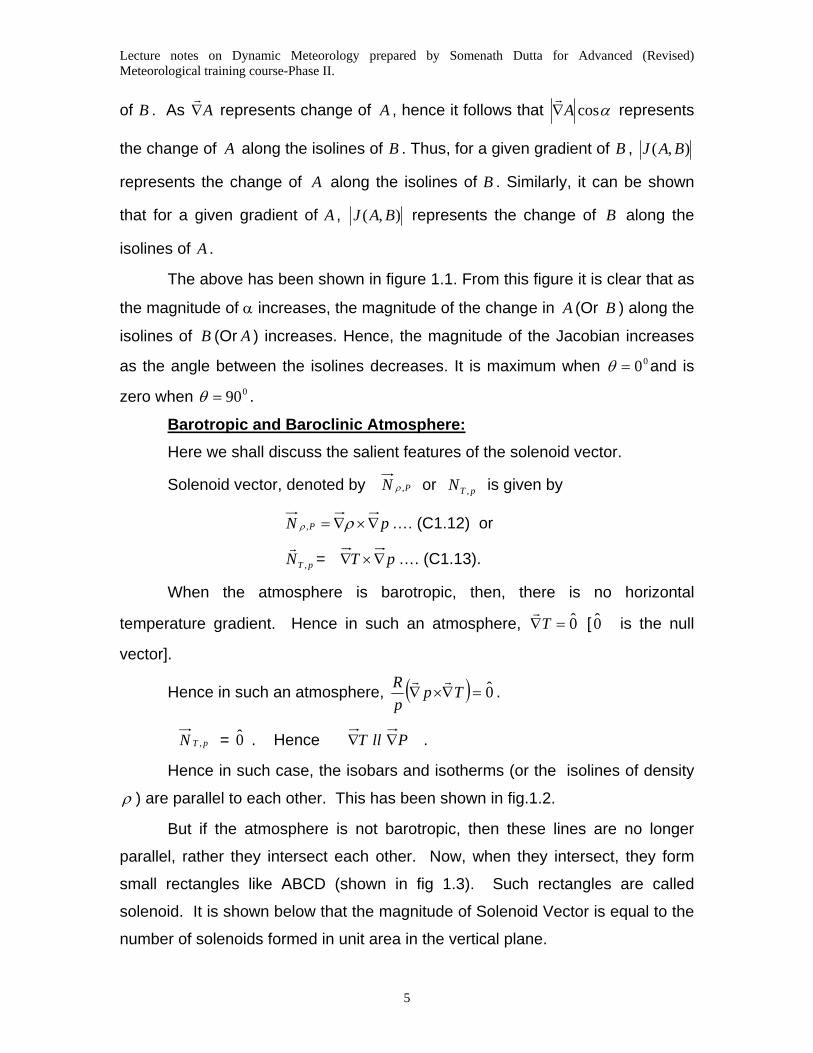
Hence in such case, the isobars and isotherms (or the isolines of density
ρ ) are parallel to each other. This has been shown in fig.1.2.
But if the atmosphere is not barotropic, then these lines are no longer
parallel, rather they intersect each other. Now, when they intersect, they form
small rectangles like ABCD (shown in fig 1.3). Such rectangles are called
solenoid. It is shown below that the magnitude of Solenoid Vector is equal to the
number of solenoids formed in unit area in the vertical plane.
Lecture notes on Dynamic Meteorology prepared by Somenath Dutta for Advanced (Revised) Meteorological training course-Phase II.
6
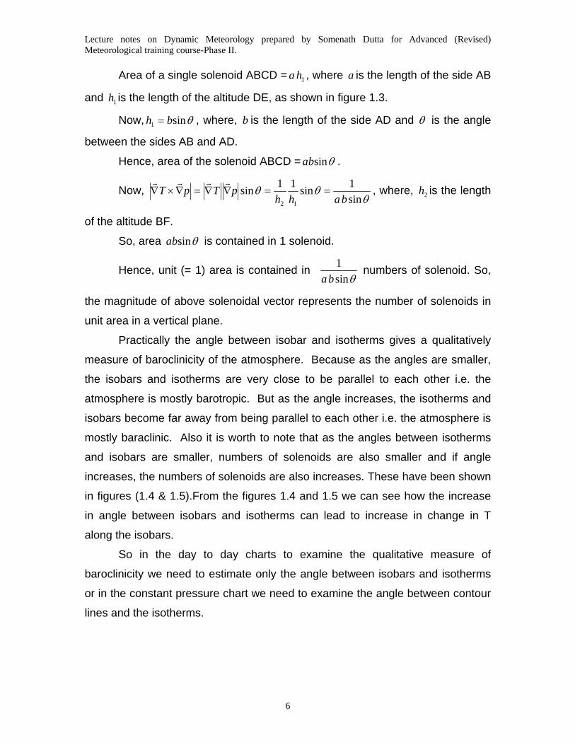
Area of a single solenoid ABCD = 1ha , where a is the length of the side AB
and 1h is the length of the altitude DE, as shown in figure 1.3.
Now, θsin1 bh = , where, b is the length of the side AD and θ is the angle
between the sides AB and AD.
Hence, area of the solenoid ABCD = θsinba .
Now, θ
θθsin1sin11sin
12 bahhpTpT ==∇∇=∇×∇rrrr
, where, 2h is the length
of the altitude BF.
So, area θsinba is contained in 1 solenoid.
Hence, unit (= 1) area is contained in θsin
1ba
numbers of solenoid. So,
the magnitude of above solenoidal vector represents the number of solenoids in
unit area in a vertical plane.
Practically the angle between isobar and isotherms gives a qualitatively
measure of baroclinicity of the atmosphere. Because as the angles are smaller,
the isobars and isotherms are very close to be parallel to each other i.e. the
atmosphere is mostly barotropic. But as the angle increases, the isotherms and
isobars become far away from being parallel to each other i.e. the atmosphere is
mostly baraclinic. Also it is worth to note that as the angles between isotherms
and isobars are smaller, numbers of solenoids are also smaller and if angle
increases, the numbers of solenoids are also increases. These have been shown
in figures (1.4 & 1.5).From the figures 1.4 and 1.5 we can see how the increase
in angle between isobars and isotherms can lead to increase in change in T
along the isobars.
So in the day to day charts to examine the qualitative measure of
baroclinicity we need to estimate only the angle between isobars and isotherms
or in the constant pressure chart we need to examine the angle between contour
lines and the isotherms.
Lecture notes on Dynamic Meteorology prepared by Somenath Dutta for Advanced (Revised) Meteorological training course-Phase II.
7
Bjerknees Circulation Theorem: Kelvin’s circulation theorem tells us about the change of absolute
Circulation. But it is more important to know about the change of circulation with
respect to the earth. Hence it is more important to know the change of relative
circulation.
Bjerkness circulation theorem tells us about the change in relative
circulation
According to Bjerkness circulation theorem, we have
dtdC
dtdC ar = -2
dtdSEΩ ………………….. (C1.14)
Proof: We know that, rVVarrrr
×Ω+= .
( )∫∫∫ ×Ω+=⇒ ldrldVldVa
rrrrrrr...
∫∫ ×Ω×∇+=⇒S
ra dsnrCC ˆ).( rrr (Stoke’s theorem used for 2nd line integral)
∫∫ Ω+=⇒S
ra dsnCC ˆ.2r
Now, φsin)ˆ,(cosˆˆ. Ω=ΩΩ=Ω nnnrrr
, where, φ is the latitude of the area
element ds and Ω=Ωr
.
Hence, ES
ra SSindsCC Ω=Ω+=⇒ ∫∫ 22 φ
Where, ∫∫ == dSdSS EE Sinφ
and ds Sinφ is the area of the projection of ds on the equatorial plane.
The first term dt
dCa , have already been discussed in the Kelvin’s circulation
theorem. Now we shall discuss the 2nd term -2dt
dSEΩ .
Considering the effect of the 2nd term independently the Bjerkness
circulation theorem gives us
)(2 112212 φφ SinSSinSCC rr −Ω−=− …………………………(C1.15)
Where 1rC = Initial relative circulation;
Lecture notes on Dynamic Meteorology prepared by Somenath Dutta for Advanced (Revised) Meteorological training course-Phase II.
8
2rC = Final relative circulation
1S = Initial area enclosed by the closed path
2S = Final area enclosed by the closed path
1φ = Initial Latitude
2φ = Final Latitude
Thus the above equation tells us that the change in relative circulation
may be due to
(i) change in area enclosed by the closed path
(ii) change in latitude
(iii) Non uniform vertical motion superimposed on the circulation
• Effect of the change in area enclosed by the closed path on the
change in relative circulation :
If the area ‘S’ enclosed by the closed path increased from S1 to S2 ,
remaining at the same latitude ’φ ’, then the resulting change in relative
circulation is given by
0)(2 1212 <−Ω−=− SSSinCC rr φ , since, S2 > S1.
Thus Cyclonic circulation decreases as the area enclosed by the closed
circulation increases. Physically it may be interpreted as follows:
Area enclosed by a closed circulation increases if and only if the
divergence increases or convergence decreases. Then due to the Coriolis force
the stream line turn anti-cyclonically or the already cyclonically turned
streamlines turn less cyclonically. As a result of which cyclonic circulation
reduces. Similarly due to convergence when the area enclosed by the circulation
decreases, the cyclonic circulation increases.
• Effect of the change in latitude on the change in relative circulation :
Now suppose a circulation moves from a lower latitude 1φ to a higher
latitude 2φ , without any change in the area enclosed by the circulation. Then the
resulting change in the relative circulation is given by
0)(2 1212 <−Ω−=− φφ SinSinSCC rr
Lecture notes on Dynamic Meteorology prepared by Somenath Dutta for Advanced (Revised) Meteorological training course-Phase II.
9
Since 12 φφ SinSin >
Hence a circulation loss its cyclonic circulation as it moves towards higher
latitude.
Similarly it can be shown that when a cyclonic circulation moves towards
lower latitude, then it gains cyclonic circulation.
• Effect of imposition of non uniform vertical motion on the change in
relative circulation.
Now consider a different situation, when neither the area enclosed by the
circulation changes nor the cyclonic circulation moves, but non uniform vertical
motion is applied to the closed circulation. Then the inclination of the plane of
rotation of circulation with the equatorial plane changes, (shown in figure 1.6) as
a result of which ES changes which leads to a change in Cr. This effect is
known as TIPPING EFFECT.
A possible explanation of sea/land breeze and thermally direct
circulation using Kelvin’s circulation Theorem:
Sea breeze takes place during day time when ocean is
comparatively cooler than land. Hence temperature increases towards land
and also we know that temperature decreases upward. (i.e. increased
downward). Thus the temperature gradient T∇r
is directed downward to the
land. For the shake of simplicity we assume that pressure over land and sea is
same, but it increases downward. Hence pressure gradient p∇r
is directed
downward. as shown in figure 1.7. Hence Tp ∇×∇rr
gives the circulation in the
direction from p∇r
to T∇r
. Also the change in circulation pattern is given by
Tp ∇×∇rr
. Hence if initially there was no circulation, then the above mentioned
pressure and temperature pattern will generate a circulation directed from p∇r
to
T∇r
, which gives low level flow from ocean to land and in the upper level from
land to ocean. This is nothing but sea breeze. Similarly land breeze and any
thermally driven circulation pattern may be explained qualitatively.
Lecture notes on Dynamic Meteorology prepared by Somenath Dutta for Advanced (Revised) Meteorological training course-Phase II.
10
VORTICITY:
Vorticity is a micro scale measure of rotation. It is a vector quantity.
Direction of this vector quantity is determined by the direction of movement of a
fluid, when it is being rotated in a plane. Observation shows that when a fluid is
being rotated in a plane, then there is a tendency of fluid movement in a direction
normal to the plane of rotation (towards outward normal if rotated anti clockwise
or towards inward normal if rotated clockwise). Thus due to rotation in the XY
plane (Horizontal plane) fluid tends to move in the k direction (i.e. vertical), due
to rotation in the YZ plane (meridional vertical plane)fluid tends to move in the i
direction (East West) and due to rotation in ZX plane (zonal vertical plane) fluid
tends to move in the j direction (N-S).
Thus vorticity has three components. Mathematically it is expressed as
ζηξ kjiV ˆˆˆ ++=×∇ ….(C1.16),
where, yu
xv
xw
zu
zv
yw
∂∂
−∂∂
=∂∂
−∂∂
=∂∂
−∂∂
= ζηξ ;; ....(C1.17).
In Meteorology, we are concerned about weather, which is due mainly to
vertical motion and also only the rotation in the horizontal plane can give rise to
vertical motion. So, in Meteorology, by the term vorticity, only the k component
of the vorticity vector is understood. Hence, throughout our study only k
component is implied by vorticity.
Thus, hence forth, vorticity = yu
xv
∂∂
−∂∂
=ζ ….(C1.18).
Relation between circulation and vorticity: We know that circulation and vorticity both are measures of
rotation. Hence it’s natural that there must be some relation between them. We
know that, circulation is given by, ldvCrr
∫= .
Hence, using Stokes theorem we have, ∫∫∫∫∫ =⋅⋅×∇=⋅= dsdskvdlvC ζ
(As in the present study, rotation is in the horizontal plane, hence, kn ˆˆ = )..
Lecture notes on Dynamic Meteorology prepared by Somenath Dutta for Advanced (Revised) Meteorological training course-Phase II.
11
Hence, ζ=dsdc …..(C1.19).Thus, vorticity is the circulation per unit area.
Vorticity for solid body rotation
Let us consider a circular disc, of radius ‘a’, rotating with a constant
angular velocity ω about an axis passing through the centre of the disc, as
shown in figure 1.8
Then the circulation of the disc = cldv =⋅∫rr (say)
Now tangential component of av ω=
And θaddl =
ωπθωθωππ
∫∫ ===∴2
0
222
0
2 2 adadac
Vorticity= Circulation/Area = ωππ 22
2
2
=a
wa ….(C1.20)
Thus for Solid body rotation, the vorticity is twice the angular velocity i.e.
2 ω.
Relative vorcity and the Planetary Vorticity
Relative vorticity = yu
xvVK r ∂
∂−
∂∂
==×∇⋅ ζ
To understand the Planetary Vorticity, we consider an object placed
at some latitude on the earth’s surface. Consider the meridional circle passing
through the object shown in figure 1.9
Then as the Earth rotates about its axis, the object executes a
circular motion (dashed circle in the fig) with radius φcosa .
Now the Circular motion executed by the object is analogous to the
solid body rotation. Hence the vorticity of the object = 2 x local vertical
component of angular velocity = fSin =Ω φ2 .
Now this vorticity is solely due to the rotation of the planet earth. Hence it
is known as planetary vorticity. It is to be noted that it is also the coriolis
parameter.
Lecture notes on Dynamic Meteorology prepared by Somenath Dutta for Advanced (Revised) Meteorological training course-Phase II.
12
Sum of relative vorticity and planetary vorticity is known as absolute
vorticity and is denoted by ‘ aζ ’
Hence aζ = f+ζ ……(C1.21)
Relative vorticity in natural co-ordinate:
In natural co-ordinate (s,n,z), we know ≡∇r
⎟⎠⎞
⎜⎝⎛
∂∂
+∂∂
+∂∂
zk
nn
st ˆˆˆ ,
where, knt ˆ,ˆ,ˆ are unit tangent, unit normal and unit vertical vector respectively.
Hence, the relative vorticity is given by
nvvKtv
zk
nn
stk s ∂
∂−=×⎟
⎠⎞
⎜⎝⎛
∂∂
+∂∂
+∂∂
= ˆˆˆˆ.ˆζ ……(C1.22)
Where, v is the tangential wind speed, sK is the streamline curvature and
nv∂∂ is the horizontal wind shear across the stream line. The first term svK of the
above expression is known as curvature vorticity and the second term nv∂∂
− is
known as Shear vorticity.
Potential vorticity
To understand the concept of Potential vorticity, first we may refer
to the popular circus play, where a girl is standing at the centre of a rotating disc.
As the girl stretches her arm, the disc rotates at a slower rate and as she
withdraws her arms the disc rotates at a faster rate. Generally this example is
referred in solid rotation to illustrate the conservation of angular momentum. This
example hints us to search a quantity in the fluid rotation, which is analogous to
the angular momentum in solid rotation.
For that we consider an air column of unit radius. Now, consider
that the air column shrinks down i.e. its depth decreases. As it shrinks down, its
radius increases and then as per the above example column will rotate at a
slower speed. Also if the air column stretches vertically i.e. if its depth increases,
then its radius decreases and rate of rotation increases
Lecture notes on Dynamic Meteorology prepared by Somenath Dutta for Advanced (Revised) Meteorological training course-Phase II.
13
So, it’s clear that the rate of rotation of the air column increases or
decreases as its depth increases or decreases.
Thus for a rotating air column, we can say that the rate of rotation is
proportional to the depth of the air column.
Now for fluid motion rate of rotation and vorticity are analogous
∴ Vorticity ∝ Depth
Vorticity/Depth = constant
Thus in the fluid rotation the quantity (Vorticity/Depth) remains constant as
in the solid rotation angular momentum remains constant. So this quantity is
analogous to the angular momentum. It is known as potential vorticity.
Therefore, Potential vorticity of an air column
= Depth
vorticityAbsolute = h
f+ζ ……(C1.23)
THE VORTICITY EQUATION:
This equation tells us about change in vorticity and the possible
mechanisms for vorticity production or destruction. This equation is derived from
the equation of horizontal motion.
Horizontal equation of motion may be re-written as
Fz
VwVkfpK
tV H
HHHHH
rr
rrrr
+∂∂
−×+−∇−∇−=∂∂ ˆ)(1 ζ
ρ…….(C1.24)
Performing ( ×∇Hkr
.ˆ ) on both sides of (C1.24), we obtain,
[ ] Fkz
VwkVkfkpkt H
HHHH
HHrr
rrrr
rr
×∇+∂∂
×∇−×+×∇−∇×∇
=∂∂ .ˆ.ˆˆ)(.ˆ.ˆ 2 ς
ρρς
To simplify the 2nd and 3rd terms on the RHS of above equation, we use
the following two vector identity
babaababba HHHHH
rrrrrrrrrrrrrrr).().().().()( ∇+∇−∇−∇=××∇
and, ( ) ( )aaa HHHrrrrrr
×∇+×∇=×∇ λλλ )(
Hence the 2nd and 3rd terms are respectively
Lecture notes on Dynamic Meteorology prepared by Somenath Dutta for Advanced (Revised) Meteorological training course-Phase II.
14
))(.()( fVfD HHH +∇−+− ςςrr
,and
zw
zV
wkVkz
wz
Vwk
zV
kwz
Vwk H
HHHH
HH
HH
H ∂∂
+⎟⎟⎠
⎞⎜⎜⎝
⎛
∂∂
×∇=×∇∂∂
+⎟⎟⎠
⎞⎜⎜⎝
⎛
∂∂
×∇=∂∂
×∇+⎟⎟⎠
⎞⎜⎜⎝
⎛
∂∂
×∇ς
rrrr
rr
rr
rr
.ˆ).ˆ(.ˆ.ˆ.ˆ
respectively, where, HHH VDrr
.∇= . Hence, the vorticity equation may be written as
⎟⎟⎠
⎞⎜⎜⎝
⎛∂∂
−∂
∂+⎟⎟
⎠
⎞⎜⎜⎝
⎛∂∂
∂∂
−∂∂
∂∂
−⎟⎟⎠
⎞⎜⎜⎝
⎛∂∂
∂∂
−∂∂⋅
∂∂
++−=+y
Fx
Fzu
yw
zv
xw
xp
yyp
xfDf
dtd xy
Hρρ
ρζζ 2
1)()( …..(C1.25)
The term on the LHS indicates the production/destruction of absolute vorticity
and the terms on the RHS indicates possible mechanisms responsible for that.
The terms on the RHS are respectively called
1) Divergence term (2) Solenoidal term
2) Tilting term and (4) Frictional term
Divergence term:- This term explains the effect of divergence/convergence on the
production/destruction of vorticity. If there is divergence then, 0>HD . Hence
considering only the effect of this term we have,
)(0)( ffdtd
+⇒<+ ςς , The absolute vorticity decreases with time.
Thus divergence cause cyclonic vorticity to decrease or anti cyclonic
vorticity to increase. This can be explained physically also. Due to divergence,
the stream line turns anti cyclonically or cyclonic turning, exists already,
decreases by the effect of Coriolis force. It is shown in figure 1.10.
Similarly, it can be shown that due to convergence [when D < 0]
)( f+ρ decreases. Thus due to convergence cyclonioc vorticity increases.
Solenoidal term:- As explained in the context of circulation theorem, here also
solenoidal term signifies the contribution of the baroclinic effect of atmosphere
towards the production or destruction of absolute vorticity.
Let us consider the first term in the solenoidal term, the
termyp
x ∂∂⋅
∂∂ρ
ρ 2
1 .
Lecture notes on Dynamic Meteorology prepared by Somenath Dutta for Advanced (Revised) Meteorological training course-Phase II.
15
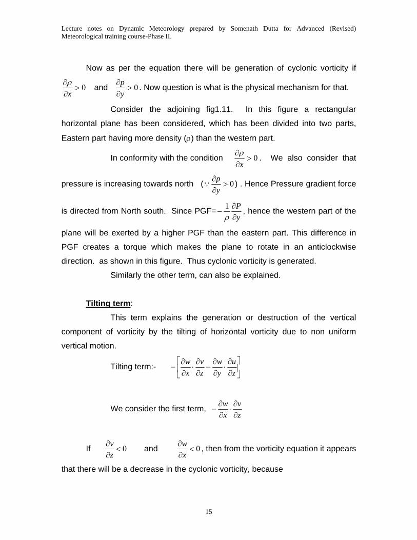
Now as per the equation there will be generation of cyclonic vorticity if
0>∂∂
xρ and 0>
∂∂
yp . Now question is what is the physical mechanism for that.
Consider the adjoining fig1.11. In this figure a rectangular
horizontal plane has been considered, which has been divided into two parts,
Eastern part having more density (ρ) than the western part.
In conformity with the condition 0>∂∂
xρ . We also consider that
pressure is increasing towards north ( 0>∂∂
yp
Q ) . Hence Pressure gradient force
is directed from North south. Since PGF=yP∂∂
−ρ1 , hence the western part of the
plane will be exerted by a higher PGF than the eastern part. This difference in
PGF creates a torque which makes the plane to rotate in an anticlockwise
direction. as shown in this figure. Thus cyclonic vorticity is generated.
Similarly the other term, can also be explained.
Tilting term:
This term explains the generation or destruction of the vertical
component of vorticity by the tilting of horizontal vorticity due to non uniform
vertical motion.
Tilting term:- ⎥⎦
⎤⎢⎣
⎡∂∂⋅
∂∂
−∂∂⋅
∂∂
−zu
yw
zv
xw
We consider the first term, zv
xw
∂∂⋅
∂∂
−
If 0<∂∂zv and 0<
∂∂
xw , then from the vorticity equation it appears
that there will be a decrease in the cyclonic vorticity, because
Lecture notes on Dynamic Meteorology prepared by Somenath Dutta for Advanced (Revised) Meteorological training course-Phase II.
16
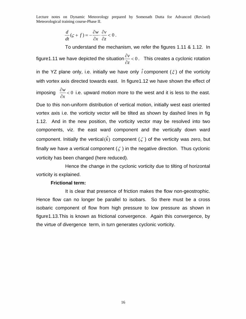
0)( <∂∂⋅
∂∂
−=+zv
xwf
dtd ς .
To understand the mechanism, we refer the figures 1.11 & 1.12. In
figure1.11 we have depicted the situation 0<∂∂zv . This creates a cyclonic rotation
in the YZ plane only, i.e. initially we have only i component (ξ ) of the vorticity
with vortex axis directed towards east. In figure1.12 we have shown the effect of
imposing 0<∂∂
xw i.e. upward motion more to the west and it is less to the east.
Due to this non-uniform distribution of vertical motion, initially west east oriented
vortex axis i.e. the vorticity vector will be tilted as shown by dashed lines in fig
1.12. And in the new position, the vorticity vector may be resolved into two
components, viz. the east ward component and the vertically down ward
component. Initially the vertical )ˆ(k component (ζ ) of the verticity was zero, but
finally we have a vertical component (ζ ) in the negative direction. Thus cyclonic
vorticity has been changed (here reduced).
Hence the change in the cyclonic vorticity due to tilting of horizontal
vorticity is explained.
Frictional term: It is clear that presence of friction makes the flow non-geostrophic.
Hence flow can no longer be parallel to isobars. So there must be a cross
isobaric component of flow from high pressure to low pressure as shown in
figure1.13.This is known as frictional convergence. Again this convergence, by
the virtue of divergence term, in turn generates cyclonic vorticity.
Lecture notes on Dynamic Meteorology prepared by Somenath Dutta for Advanced (Revised) Meteorological training course-Phase II.
17
Scale analysis of vorticity equation: What is scale analysis? Before that we should have a clear concept about ‘Order of magnitude’. Suppose that the observed wind speed is between 6 m/sec to 50
m/sec, then we say order of magnitude of observed wind speed is 10 m/sec.
Ranges of values(m/s)
Order of Magnitude(m/s)
1- 5 010 6-50 110 51-500 210 501-5000 310 etc.
Scale analysis is a convenient technique to compare the relative order of
magnitude of individual terms of governing equation, from the knowledge of the order of magnitude of field variables, then retaining only the terms with highest order of magnitude discarding others and their by simplifying the governing equation.
For performing scale analysis the following steps are to be taken:
i) Typical order of magnitude of the individual field variables. (like u, v, T, p, x, y etc) are found out from the field observations.
ii) Then the relative orders of magnitude of the individual term of governing equations are found out.
iii) Only the terms with highest order or magnitude are retained and others are discarded. Scale analysis of the vorticity equation: First term of the LHS of vorticity equation may be expanded as
)()()()(1))(( 2 RHSyF
xF
zu
yw
zu
xw
xp
yyp
xf
yv
xu
yfv
zw
yv
xu
t
xy ⇒∂∂
−∂∂
+∂∂
∂∂
−∂∂
∂∂
−∂∂⋅
∂∂
−∂∂⋅
∂∂
++∂∂
+∂∂
−=
∂∂
+∂∂
+∂∂
+∂∂
+∂∂
ρρρ
ζ
ζζζζ
Lecture notes on Dynamic Meteorology prepared by Somenath Dutta for Advanced (Revised) Meteorological training course-Phase II.
18
Following all the necessary steps of scale analysis, we find that the terms
zw
yv
xu
t ∂∂
∂∂
∂∂
∂∂ ζζζζ ,,, on the LHS of vorticity equation and the only term
)(yv
xuf
∂∂
+∂∂
− on the RHS are having order of magnitude, 21010 −− Sec Sec and
all the other terms are having order of magnitude less than 21010 −− Sec . Hence following the principle of scale analysis we can retain only
those terms with order of magnitude 21010 −− S and other terms may be discarded.
Hence the vorticity equation may be simplified into
βζζζ vyv
xuf
yv
xu
t−
∂∂
+∂∂
−=∂∂
+∂∂
+∂∂ )(
Where yF∂∂
−=β
)(][yv
xufv
yv
xu
t ∂∂
+∂∂
−+∂∂
+∂∂
−=∂∂ βζζζ
Vorticity advection of Horizontal div. Tendency relative vorticity By hori. wind
)()( HHH DffVt
−+∇⋅−=∂∂ ζζ ………………….(C1.26)
This equation is very much useful to explain the divergence pattern
on different sectors of Jet core and also to explain the divergence pattern associated with trough
Question.: Why divergences occur to the ahead of a westerly trough? For that first write the above equation (C1.26).
)()( HHH DffVt
−+∇⋅−=∂∂ ζζ
Under steady state condition, 0=∂∂
tς .
Lecture notes on Dynamic Meteorology prepared by Somenath Dutta for Advanced (Revised) Meteorological training course-Phase II.
19
Hence, f
fVD HH
H)(. +∇−
=ς
rr
. Now the denominator of this expression is
called advection of vorticity. It may be +ve (cyclonic) or –ve (anticyclonic) accordingly as wind is coming from the source of cyclonic vorticity or anticyclonic vorticity. If in a region wind comes from a source of cyclonic vorticity, then in that region cyclonic vorticity is brought and on the other hand if in that region wind comes from a source of anticyclonic vorticity, then in that region anticyclonic vorticity is brought.
Now we consider a typical stationary westerly trough (figure 1.14). Consider a region (C) behind the trough and the region (D) ahead of the trough. In the region (D) winds are coming from the trough, a source of cyclonic vorticity. Hence in this region advection of cyclonic vorticity is taking place.
Hence .0)( >+∇⋅− fV HH ζ Hence in this region,
=HfD .0)( >+∇⋅− fV HH ζ 0>∴ HD , implying that at 300 mb divergence takes place in this region.
Hence low pressure area forms at the surface area ahead of an upper air trough. Similarly in (C) region winds coming from a ridge, a source of anticyclonic
vorticity, hence anticyclonic vorticity advection takes place over this region. Hence in this region
0)( <+∇⋅− fV HH ζr
; so 0)()( <+∇⋅−= fVDf HHH ζ 0<∴ HD , so there is convergence behind the trough at 300 hPa,
so high pressure area forms at the surface behind an U.A. trough. We shall discuss the divergence pattern in different sectors of Jet Stream.
To discuss the divergence pattern in different sectors of the sub-tropical westerly jet stream, we may refer figure 1.15. In this figure four sectors have been shown
Sector I (Left exit) In this sector we have considered two points P & Q, P being nearer
the core and Q being away from Jet core. We compute the vorticity at these two points using natural co-
ordinate. In the natural co-ordinate system, vorticity ζ is given by
nVVKs ∂∂
−=ζ ; sK being the Stream line Curvature, here 0=sK as the
stream lines are almost straight line for Jet stream.
nV∂∂
−=∴ζ
Now in this sector, at the point P = + 27.5 Unit and Q = 22.5 unit, But the direction of wind is from P to Q ie. wind is coming from higher cyclonic vorticity to lower cycloniv vorticity. Hence in this case advection is cyclonic vorticity .
0)( >+∇⋅−∴ fV HH ζ
Lecture notes on Dynamic Meteorology prepared by Somenath Dutta for Advanced (Revised) Meteorological training course-Phase II.
20
=∴ )( HDf .0)( >+∇⋅− fV HH ζ So, 0>HD
Hence divergence takes place at the Jet Core Level in the Left exit sector I. Following a similar approach, divergence pattern in other sectors may also be found. Barotropic or Rossby potential vorticity: We consider a fluid flow in an infinite channel, bounded below by the earths surface and above by a rigid lid (for example, tropopause). For such fluid flow, normal component of fluid at any point is zero, i.e., at any point, 0=nV . Hence,
from Gauss’s divergence theorem we have, ( ) ∫∫∫∫∫ ==∇s
n dsVdV 0.σ
σrr
. Hence such
flow is non divergent. Hence, for such flow the scaled vorticity equation reduces to:
zwf
dtfd
∂∂
+=+ )()( ςς . Since, the flow is non-divergent, we may ignore the effect
of ageostrophic part of horizontal wind. Also we consider a barotropic atmosphere. Under these conditions, vertical integration of the above equation from bzz = to
tzz = leads to
dtdh
dtzd
dtzd
zwzwdt
fdf
h btbt =−=−=
++
)()()()(
ςς
, where, bt zzh −= is the depth
of the fluid. The above equation after integration with time further simplified to
=+h
fς Constant. This quantity is known as Barotropic or Rossby potential
vorticity. This is known as conservation of Barotropic potential vorticity. For non-divergent flow at any level, scaled vorticity equation reduces to
0)(=
+dt
fd ς , i.e., =+ fς constant. Trajectory of an air parcel conserving
absolute vorticity is known as Constant Absolute Vorticity (CAV) trajectory. It can be shown that this trajectory is looked wave like. Baroclinic or Ertel’s potential vorticity To obtain an expression for Baroclinic or Ertel’s potential vorticity, we start from horizontal equation of motion in ),,,( tyx θ co-ordinate. We know that vector form of the horizontal equation of motion in isobaric co-ordinate is given by
( ) HHPH
HPHH FVkf
pV
VVt
V rrrr
rrrr
+×+∇−=∂∂
+∇+∂∂ ˆ. φω
Lecture notes on Dynamic Meteorology prepared by Somenath Dutta for Advanced (Revised) Meteorological training course-Phase II.
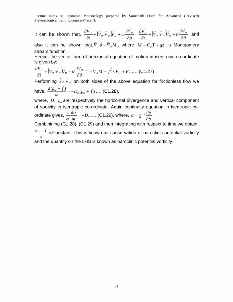
21
It can be shown that, ( ) ( )θ
θω θ ∂∂
+∇+∂∂
=∂∂
+∇+∂∂ H
HHHH
HPHH V
VVt
Vp
VVV
tV
r&
rrrrr
rrrr
.. and
also it can be shown that, MP θφ ∇=∇rr
, where gzTCM P += is Montgomery stream function. Hence, the vector form of horizontal equation of motion in isentropic co-ordinate is given by:
( )θ
θθ ∂∂
+∇+∂∂ H
HHH VVVt
Vr
&rrr
r
. = HH FVkfMrrr
+×+∇− ˆθ …..(C1.27)
Performing θ∇×r
k on both sides of the above equation for frictionless flow we
have, )()(
fDdt
fd+−=
+θθ
θ ςς …..(C1.28),
where, θθ ς,D are respectively the horizontal divergence and vertical component of vorticity in isentropic co-ordinate. Again continuity equation in isentropic co-
ordinate gives, θσ
σD
dtd
−=1 …..(C1.29), where,
θσ
∂∂
= − pg 1 .
Combinining (C1.28), (C1.29) and then integrating with respect to time we obtain
=+σ
ςθ f Constant. This is known as conservation of baroclinic potential vorticity
and the quantity on the LHS is known as baroclinic potential vorticity.
Lecture notes on Dynamic Meteorology prepared by Somenath Dutta for advanced (old) meteorological training course.
1
Chapter-II
PERTURBATION THEORY
Main goal in Meteorology is to forecast the weather parameters for the future time
with the knowledge of their present value. Bjerkness (1904) had recognized this problem
of weather forecasting as an initial value problem(IVP).
Initial value problem is a partial differential equation (Linear/ Non-Linear) with
time (t) as an in dependent variable.
Some Useful Concepts :
Partial derivative:
Let a quantity ‘S’ is dependent on x, y, z, t. Then derivative of S with respect to
any one (say t) of these four, keeping rest three unchanged, is called partial derivative of
S with respect to ‘t’. For example 24 hrs change of pressure at a place is the partial
change in pressure with respect to time. These are denoted by zs
ys
xs
ts
∂∂
∂∂
∂∂
∂∂ ,,, etc.
Examples: Let, axyzyxV 333 ++=
Hence, ayzxxV 33 2 +=∂∂ (y, z have been kept constant)
axzyyV 33 2 +=∂∂ (z, x have been kept constant)
axyzV 3=∂∂ (x, y have been kept constant)
Partial differential equation (PDE):
A differential equation is an equation which involves derivative or differential of
the dependent variable. A PDE is an equation which involves partial derivatives or
differentials of the dependent variable.
EX: fvxp
yuv
xuu +
∂∂
−=∂∂
+∂∂
ρ1 is a partial differential equation, as it contains the
partial derivatives of the dependent variables ., pu
Order of a PDE :
It is the highest order partial derivatives involved in the equation.
Lecture notes on Dynamic Meteorology prepared by Somenath Dutta for advanced (old) meteorological training course.
2
Ex. Consider the PDE ),(2
2
2
2
yxFyu
xu
=∂∂
+∂∂ .
Here, u is the dependent variable, x, y are independent variables and F(x ,y) is a
known function of x,y. In the PDE the highest order partial derivative involved in this
equation is 2. So the order of this PDE is 2.
Linear and non-linear PDE :
A general form of a 2nd order PDE is given by
GFuyuE
xuD
yuC
yxuB
xuA =+
∂∂
+∂∂
+∂∂
+∂∂
∂+
∂∂
2
22
2
2
.
In the above equation A,B,C,D,E,F and G are called coefficients of the PDE. If all
these coefficients are constants or functions of independent variables ( x , y), then the
resulting PDE is known as a Linear PDE.
For example let us consider the following PDE:
02 2
22
2
2
=∂∂
+∂∂
∂+
∂∂
yu
yxu
xu .
For this PDE A = 1
B = 2
C = 1 and
D = E = F = G=0. Hence this PDE is a Linear PDE.
We consider another PDE,
)(2 2
22
2
2
22 yx
yux
yxuxy
xuy +=
∂∂
+∂∂
∂+
∂∂ . In this PDE, A, B, C and G are functions
of x or y or both. So, this is also a 2nd order linear PDE.
on the other hand if at least one these coefficients is a function dependent
variable, then the resulting PDE is known as a non-linear PDE.
For example let us consider the following PDE:
xp
yuv
xuu
∂∂
−=∂∂
+∂∂
ρ1 .
In the above equation, A = B = C = F = 0, D = u and E = v. Since u, v are
dependent variables, hence it is a non-linear PDE.
Need for the perturbation theory :
Lecture notes on Dynamic Meteorology prepared by Somenath Dutta for advanced (old) meteorological training course.
3
There are several method for weather forecasting, viz. synoptic, statistical,
Dynamic (Numerical weather prediction) method etc.
In the NWP, the governing equations are solved for the weather parameter, viz.
u,v,w, T, P etc.. The governing equations are non-linear partial differential equation.
Non-linear partial differential equations can not be solved exactly, as till now we don’t
have any method to get exact solution of non-linear partial differential equation.
To get rid of the above problem, there are two ways viz.,
(a) Transform the non-linear partial differential equation into ordinary
differential equation and then get exact solution.
(b) Transform the set of partial differential equations into their finite
difference form and then solve them numerically.
Discussion about (a) is beyond the scope of discussion. Now while discussing
(b), it is worth mentioning that the numerical solution of these non-linear partial
differential equation is highly sensitive to the initial conditions given, i.e. a slight change
in the initial condition may lead to an abrupt change in the numerical solution. This is
due to the presence of non-linearity in the governing equations. Perturbation theory was
proposed to remove the non-linearity from the governing equations.
Basic postulates of perturbation theory :
This theory is based on same postulates, which are given below :
I. According to this theory, the total atmospheric flow consists of a mean flow
and a perturbation superimposed on it. So, that all field variables consist of a
basic (mean) part and a perturbation part.
II. Both the mean part and the total (mean + perturbation) satisfy the governing
equations. Mean part is the temporal and longitudinal average of the variable
as a result of which it is independent of x and t.
III. The magnitude of perturbation part is very small as compared to that of mean
part, so that any product of perturbations or product of their derivatives or
product of a perturbation and derivative of perturbation may be neglected.
Now, it is our task, to verify whether using the above postulates, the non-linearity
from a
term of governing equation may be removed or not.
Lecture notes on Dynamic Meteorology prepared by Somenath Dutta for advanced (old) meteorological training course.
4
For that we consider an arbitrary non-linear term, say, x
u∂∂ϕ .
Using postulate (I), uuu ′+= and ϕϕϕ ′+= .
Hence, x
ux
uxx
uux
uux
u∂′∂′+
∂′∂
=⎟⎟⎠
⎞⎜⎜⎝
⎛∂′∂
+∂∂′+=
∂′+∂′+=
∂∂ ϕϕϕϕϕϕϕ )()()( (Here,
0=∂∂
xϕ , as per 2nd part of postulate (II)). Again using postulate (III), 0≈
∂′∂′
xu ϕ , being a
product of perturbation quantity and its derivative.
Hence using perturbation technique, non-linearity from the governing equations
may be removed.
Lecture notes on Dynamic Meteorology for Revised Advanced training course prepared by Dr.Somenath Dutta.
Mechanisms of pressure change Pressure tendency equation: To derive pressure tendency equation, we shall start from the hydrostatic approximation
ρgzp
−=∂∂ …….(1)
Integrating the above equation vertically from an arbitrary level to , we obtain,
0zz = ∞=z
∫∫∞
=
∞
=
−=∂∂
00 zzzz
dzgdzzp ρ
∫∞
=⇒0
)( 0z
dzgzp ρ , since, at the top of the atmosphere there is no pressure.
Now, differentiating the both sides of the above partially with respect to time, we obtain,
∫∫∞∞
∂∂
=⎟⎟⎠
⎞⎜⎜⎝
⎛
∂∂
=∂∂
00 zz
dzt
gdzgtt
p ρρ
Again from continuity equation we have, ).( Vt
rrρρ
∇−=∂∂
So, we have, ( ) )()(.).(
).(
00
00
0
zwzgdzVgdzVg
dzVgtp
zhh
zhh
z
ρρρ
ρ
+∇−+∇−=
∇−=∂∂
∫∫
∫∞∞
∞
rrrr
rr
The above equation is known as pressure tendency equation. Left hand side of the above equation represents pressure tendency at a point at level 0zz = and right hand side consists of three terms each of which representing some mechanisms for pressure change.
First term is known as divergence term. It represents net lateral divergence or convergence across the sidewall of an atmospheric column with base at and extending up to top of the atmosphere. We know that pressure at
0zz =
0zz = is nothing but the weight of air contained in an atmospheric column with base at 0zz = having unit cross sectional area and extending up to top of the atmosphere. Now this weight will increase or decrease if mass of air inside this column increases or decreases. Again mass of air inside this column increases or decreases if there is net inflow (convergence) or out flow (divergence) of air. Hence, net lateral divergence leads to fall in pressure and net lateral convergence leads to a rise in pressure. For synoptic scale system, this term contributes significantly towards pressure change.
Second term expresses the net lateral advection of mass into the atmospheric column with base at having unit cross sectional area and extending up to top of the atmosphere. Clearly net positive advection leads to an increase in mass, which in tern leads to rise in pressure and net negative advection leads to a decrease in mass which in tern leads to fall in pressure.
0zz =
Third term expresses flux of mass into the above atmospheric column across its base at . 0zz =
Lecture notes on Dynamic Meteorology for Revised Advanced training course prepared by Dr.Somenath Dutta.
Movement of different pressure systems: Here we shall discuss the movement of pressure systems (lows/highs) for different isobaric patterns. Mainly we shall discuss Sinusoidal pattern, circular pattern and circular pattern beneath a Sinusoidal pattern above.
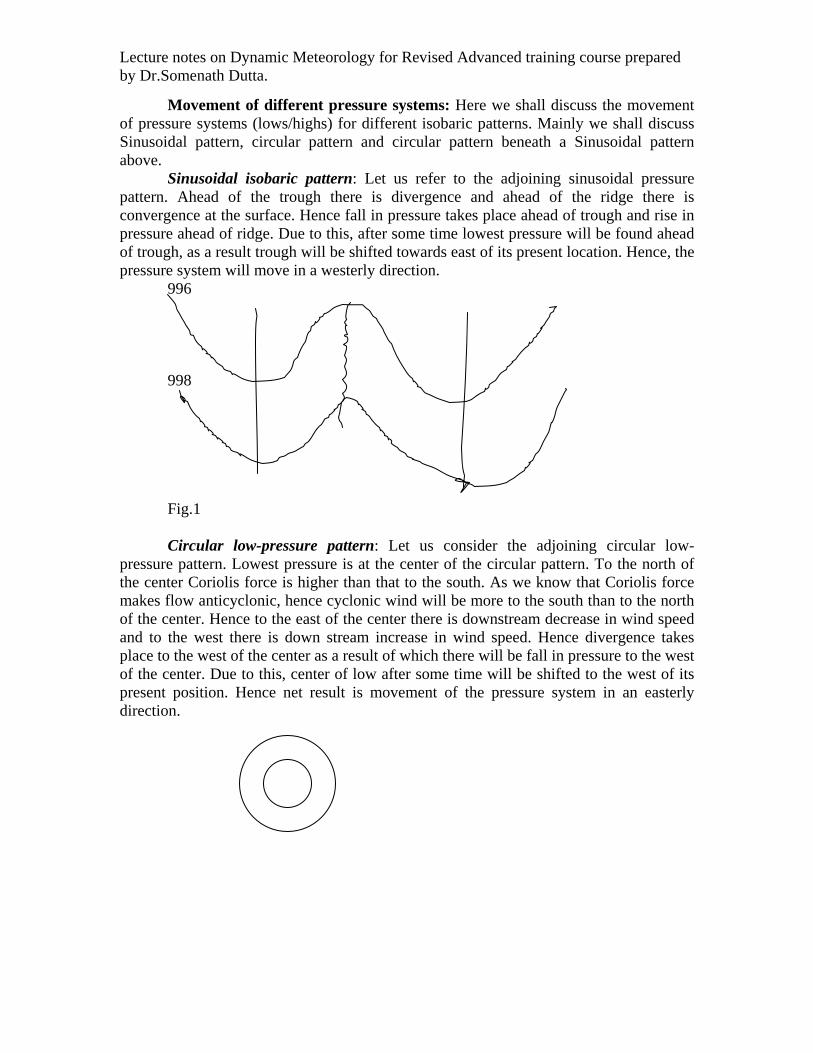
Sinusoidal isobaric pattern: Let us refer to the adjoining sinusoidal pressure pattern. Ahead of the trough there is divergence and ahead of the ridge there is convergence at the surface. Hence fall in pressure takes place ahead of trough and rise in pressure ahead of ridge. Due to this, after some time lowest pressure will be found ahead of trough, as a result trough will be shifted towards east of its present location. Hence, the pressure system will move in a westerly direction.
996 998 Fig.1 Circular low-pressure pattern: Let us consider the adjoining circular low-
pressure pattern. Lowest pressure is at the center of the circular pattern. To the north of the center Coriolis force is higher than that to the south. As we know that Coriolis force makes flow anticyclonic, hence cyclonic wind will be more to the south than to the north of the center. Hence to the east of the center there is downstream decrease in wind speed and to the west there is down stream increase in wind speed. Hence divergence takes place to the west of the center as a result of which there will be fall in pressure to the west of the center. Due to this, center of low after some time will be shifted to the west of its present position. Hence net result is movement of the pressure system in an easterly direction.
Lecture notes on Dynamic Meteorology prepared by Somenath Dutta for advanced (old) meteorological training course.
Chapter-III
ATMOSPHERIC WAVES:
Wave may be defined as a form of disturbance in a medium.
When a disturbance is given to a part of an elastic medium, then
that part gets displaced from its original position. But by the virtue of elasticity, a
restoring force is developed in the displaced part, which helps it to return to its
original position. This leads to an oscillatory motion, which is known as wave.
Some useful concepts on waves:
WAVE LENGTH:
It is defined as the distance between two consecutive points on the
wave, which are in the same phase of oscillation, i.e. distance between two
successive troughs or ridges.
WAVE NUMBER:
Wave number of a wave with wave length ‘L’ is defined as the
number of such waves exist around a circle of unit radius. Hence wave number
k is defined by, L
k π2= , where L is the wave length.
Since a wave may travel in any direction, hence we may define
wave length / wave number for three directions, viz. along x, y and z directions.
If yx LL , and zL are respectively the wave lengths along x, y and z
directions and if lk, and m are wave numbers along x, y and z directions, then
yx L
lL
k ππ 2,2== and
zLm π2= .
FREQUENCY :
It is the number of wave produced in one second.It is denoted by ν.
PHASE VELOCITY:
We know that any disturbance behaves like a carrier. So, wave
may be thought of as a carrier. Phase velocity is defined as the rate at which
Lecture notes on Dynamic Meteorology prepared by Somenath Dutta for advanced (old) meteorological training course. momentum is being carried by the wave. For practical purpose, it may be taken
as the speed with which a trough / ridge moves.
It can be shown that, phase velocity in any direction = frequency / wave
number in that direction. Thus if the phase velocity vector Cr
has components
Cx, Cy, Cz along x, y and z direction, then lCkC yx /,/ νν == and mCz /ν= .
GROUP VELOCITY :
It is the rate at which energy is being carried by the wave. When a single wave
travels then the energy and momentum are carried by the wave at the same rate. But
when a group of wave travel then momentum propagation rate and energy propagation
rates are different. So, in such case group velocity and phase velocity are different. Thus
if the phase velocity vector GCr
has components CGX, CGY, CGZ along x, y and z
direction, then l
Ck
C GYGX ∂∂
=∂∂
=νν , and
mCCZ ∂
∂=
ν .
DISPERSION RELATION :
It is a mathematical relation ),,( mlkf=ν between the frequency ( ν
) and wave numbers mlk ,, .
Generally for any wave, phase velocity and group velocity is
obtained from the dispersion relation.
If for any wave phase velocity and group velocity are same, then it
is called a non-dispersive wave, otherwise it is a dispersive wave.
ROSSBY WAVE:
First it will be shown how conservation of absolute vorticity (ζ+f)
leads to wave like motion.
We consider an object placed on or over the earths surface at
latitude ‘ϕ’ . In the adjoining figure, a meridional circle passing through the
Lecture notes on Dynamic Meteorology prepared by Somenath Dutta for advanced (old) meteorological training course. object has been shown. Suppose, while motion, the absolute vorticity (ζ+f) of
the object remains conserved. Let the object be at stationary state initially.
Then the relative vorticity ( ζ ) of the object is zero at the initial state. Let
f 1 be the value of planetary vorticity at the initial state. Now if the object be
displaced meridionally, then its relative vorticity will change to ζf (say). If f2 be
the value of planetary vorticity (f) at the final state, then we must have
yyyffffff ff βδδδςς −=∂∂
−=−=−−=⇒+=+ )(0 1221 .
Hence, 0>fς , if δy < 0, i.e., for a southward displacement and
0<fς , if δy > 0, i.e., for a northward displacement.
So, if the object is displaced northward, then it turns anti-
cyclonically towards its initial latitude. At the initial latitude ζf = O, but by inertia it
will continue to move southward, cross the initial latitude and acquire cyclonic
vorticity. After acquiring cyclonic vorticity, the object turns towards its original
latitude. Thus the object executes wave like motion about its initial latitude ‘ϕ’ .
This wave is known as Rossby wave.
Thus the dynamical constraint for Rossby wave is the conservation
of absolute vorticity.
So, to obtain the dispersion relation for the Rossby wave, the governing
equation is conservation of absolute vorticity , i.e.
0)(=
+dt
fd ς 0. =+∇+∂∂
⇒ βςς vVt
rr…..(1)
The above equation is linearised using perturbation method. Here we
made the following assumptions :
Atmosphere is auto-barotropic
Basic flow is zonal
Basic zonal flow is meridionally uniform
Lecture notes on Dynamic Meteorology prepared by Somenath Dutta for advanced (old) meteorological training course.
With these assumptions, the above governing equation may be linearised
to
0=′+∂′∂
+∂′∂ βςς v
xU
t….(2)
ς ′ is perturbation relative vorticity and v′v’ is perturbation meridional wind.
For equation (2) we seek for wave like solution, like, )()( tcxkie −∝′ , where,
k is the zonal wave number and c is the zonal phase velocity.
After simplification we obtain following dispersion relation , k
kU βν −= .
Hence phase velocity C = 2kU
kβν
−= and group velocity CG = 2kU
kβν
+=∂∂ .
Clearly GCC ≠ . So, Rossby wave is a dispersive wave.
Since 2kUC β
−=− , hence Rossby wave retrogates with respect westerly
mean flow. Again 02 >=−k
UCGβ . Hence Rossby wave carries energy in the
downwind direction with respect to westerly mean flow. Physically the above
results may be interpreted as follows: For momentum source is the westerly
mean flow and for energy the source is the disturbance i.e., the wave.
HAURWITZ WAVE :
This wave is a generalization of the Rossby wave. Similar to
Rossby wave, this wave also results from the conservation of absolute vorticity.
To obtain the dispersion relation for this wave we take the same assumptions as
in Rossby wave except that, here we assume that the basic zonal flow ‘U’ is not
uniform in the meridional direction, rather it is a function of ‘y’ (latitude) and
amplitude of this wave is zero at y = ± d, i.e., U(± d) = 0.
Starting with the conservation of absolute vorticity, and following
the approach, similar to that, made in Rossby wave, we arrive at the following
dispersion relationship.
Lecture notes on Dynamic Meteorology prepared by Somenath Dutta for advanced (old) meteorological training course.
⎟⎟⎠
⎞⎜⎜⎝
⎛+
⎟⎟⎠
⎞⎜⎜⎝
⎛−
−=
2
22
2
2
4dk
kdz
Ud
kUπ
βν
Clearly if the zonal basic flow ‘U’ is uniform in the meridional
direction, then 02
2
=dz
Ud and d → ∞ . In that case k
kU βν −= .This is nothing but
the dispersion relationship for Rossby wave. So, the Haurwitz wave is a
generalisation of Rossby wave.
GRAVITY WAVE
We have seen that to generate any wave always a restoring force
is required. Gravity waves are those waves, for which he restoring force is
buoyancy.
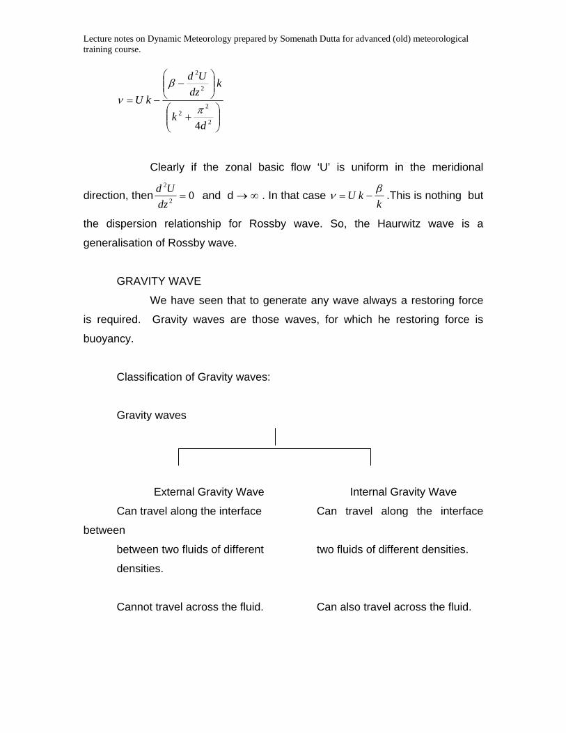
Classification of Gravity waves:
Gravity waves
External Gravity Wave Internal Gravity Wave
Can travel along the interface Can travel along the interface
between
between two fluids of different two fluids of different densities.
densities.
Cannot travel across the fluid. Can also travel across the fluid.
Lecture notes on Dynamic Meteorology prepared by Somenath Dutta for advanced (old) meteorological training course.
Vertical scale is negligible Vertical scale is comparable to
the
Compared to horizontal scale horizontal scale of motion
of motion
Eg. Sea waves, Tsunami Eg. Mountain wave, etc.
EXTERNAL GRAVITY WAVE (EGW)
To study the external gravity wave, we consider two different fluids
of densities 1ρ and 2ρ ( 1ρ > 2ρ ) placed one over the other. In the undisturbed
condition their interface is a plane surface whose vertical section is a horizontal
line as shown in figure 3(a). Now if any perturbation is given to the interface,
then it would no longer be a plane surface, rather a wavy surface. Its vertical
section would be a wave as shown in fig. 3(b). To study this wave, we consider
wave motion in the x-z (Zonal-vertical) plane, as shown in fig. 3(c).
The governing equations are:
• u-momentum equation,
• continuity equation.
These equations are linearized using perturbation method. Then
wave like solution is sought for the perturbation height of the interface. Then
after simplification we obtain the following dispersion relation.
1ρρν ∆
±= gHkUk , where, H is the mean depth of the free surface,
ρ∆ = 1ρ - 2ρ .
Now if we take air over ocean water, then definitely 1ρ >> 2ρ and
ρ∆ = 1ρ - 2ρ ≈ 1ρ , and in that case gHkUk ±=ν
Hence, phase speed gHUk
C ±==ν
Lecture notes on Dynamic Meteorology prepared by Somenath Dutta for advanced (old) meteorological training course.
And group velocity gHUk
CG ±=∂∂
=ν .
Hence C = CG
So, EGW is a non-dispersive wave.
Here gH is known as shallow water gravity wave speed and U
is known as Doppler shift.
Internal gravity wave (IGW) :
To study IGW we consider, for simplicity, a flow which is,
• 2 – D (x-z)
• Adiabatic
• Frictionless
• Non – rotational
• Boussinesq.
The governing equations are:
• U-momentum equation
• W-momentum equation
• Continuity equation
• Energy equation under adiabatic condition.
The above equations are linearised using perturbation method.
The linearised form of the above equations are :
xp
xuU
tu
∂′∂
−=∂′∂
+∂′∂
0
1ρ
00
1θθ
ρ′
+∂′∂
−=∂′∂
+∂′∂ g
zp
xwU
tw
Lecture notes on Dynamic Meteorology prepared by Somenath Dutta for advanced (old) meteorological training course.
0=∂′∂
+∂′∂
zw
xu
0=∂′∂
+∂′∂
xU
tθθ
Wave solutions, for the perturbations in the above equations are sought.
Wave solutions are like [ ])(exp tmzkxi ν−+
Then after same simplifications we obtain the following dispersion
relationship
22 mk
NkkU+
±=ν .
Phase velocity :
X-Component of phase velocity 22 mk
NUk
Cx+
±==ν ,
Z-Component of phase velocity 22 mkm
NkmkU
mCz
+±==
ν .
Group velocity:
X-Component of group velocity 22
2
mkNmU
kCGx
+±=
∂∂
=ν ,
Z-Component of group velocity ⎟⎟⎠
⎞⎜⎜⎝
⎛
+±−=
∂∂
=22 mk
Nkmm
CGzν .
Now we consider a special case for U = 0
Then22 mkm
NkCz+
±= and ⎟⎟⎠
⎞⎜⎜⎝
⎛
+±−=
22 mkNkmCGz
Lecture notes on Dynamic Meteorology prepared by Somenath Dutta for advanced (old) meteorological training course.
Thus it follows that for a given combination of signs of ;,, lk ZC and GZC are
opposite to each other. Thus vertical phase propagation (momentum
propagation) and group propagation (energy propagation) by IGW are opposite
to each other.
Also from the above expressions of C’s and CG ‘s it follows that the vector
YX CjCiC ˆ+=)r
is perpendicular to the phase lines =−+ tmzkx ν constant, where
as the vector GYGXG CjCiC ˆ+=)r
is parallel to the phase lines
=−+ tmzkx ν constant.
Hence for the IGW, phase velocity and group velocity are
perpendicular to each other.
Importance of IGW:
IGW, although, is generated at lower troposphere, they can transport
energy, momentum etc upto a great height. From the expressions for phase
velocity and group velocity, it is seen that a vertically propagating IGW extracts
Westerly Momentum from the mean flow at upper level or imparts easterly
momentum to the mean flow at upper level.
IGW is believed to be one of the causes responsible for QBO. CAT is
believed to be also due to continuous extraction of momentum from upper level
Lecture notes on Dynamic Meteorology prepared by Somenath Dutta for advanced (old) meteorological training course. mean flow by
Chapter-IV
Planetary Boundary Layer (PBL)
A Brief essay on PBL:
PBL is the lower most portion of the atmosphere, adjacent to the earth’s surface, where maximum
interaction between the Earth surface and the atmosphere takes place and thereby maximum exchange of
Physical properties like momentum, heat, moisture etc., are taking place.
Exchange of physical properties in the PBL is done by turbulent motion, which is a characteristic
feature of PBL. Turbulent motion may be convectively generated or it may be mechanically generated.
If the lapse rate near the surface is super adiabatic, then PBL becomes positively Buoyant,
which is favourable for convective motion. In such case PBL is characterized by convective turbulence.
Generally over tropical oceanic region with high sea surface temperature this convective turbulence occurs.
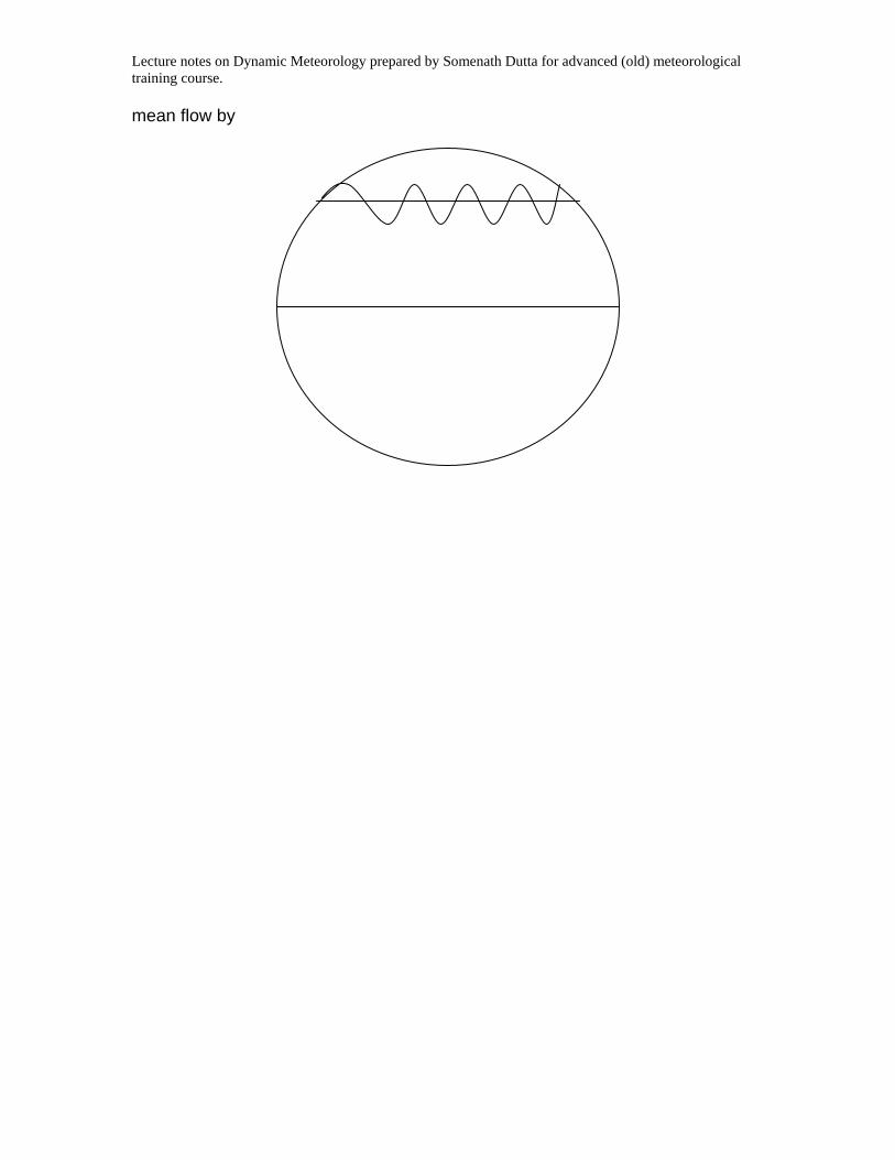
If the lapse rate near the surface is sub adiabatic then the PBL is negatively buoyant and it is not
favourable for convective turbulence. But in such case, if there is vertical shear of horizontal wind, then
Vortex (cyclonic or anti cyclonic) sets in, in the vertical planes in PBL, as shown in the adjacent fig 2b.
This vortex motion causes turbulence in the PBL, known as mechanical turbulence.
If the PBL is positively buoyant as well as, if vertical shear of the horizontal wind exists, then both
convective and Mechanical turbulence exits in the PBL. The depth of the PBL is determined by the
maximum vertical extent to which the turbulent motion exists in PBL. On average it varies from few cms
to few kms. In case of thunderstorms PBL may extend up to tropopause.
Generally at a place on a day depth of PBL is maximum at noon and in a season it is maximum
during summer.
Division of the PBL into different sub layers:
The PBL may be sub divided into three different sections, viz viscous sub layer, the surface layer
and the Ekmann layer or entrainment layer or the transition layer.
Viscous layer is defined as the layer near the ground, where the transfer of physical quantities by
molecular motions becomes important. In this layer frictional force is comparable with PGF.
The surface layer extends from z = 0z (roughness length) to szz = with sz , the top of the surface
layer, usually varying from 10 m to 100 m. In this layer sub grid scale fluxes of momentum (eddy stress)
and frictional forces are comparable with PGF.
The last layer is the Ekmann layer is defined to occur from sz to iz , which ranges from 100 m or
so to several kilometers or more. Above the surface layer, the mean wind changes direction with height
and approaches to free stream velocity at the height z as the sub grid scale fluxes decrease in magnitude. In
this layer both the COF and Eddy stress are comparable with PGF.
2
Boussinesq approximation: According to this approximation density may be treated as constant
everywhere in the governing equations except in the vertical momentum equation, where it is coupled
with Buoyancy term. Physically this approximation says that the variation of density in the horizontal
direction is insignificant as compared to that in the vertical direction.
Governing equations in the PBL: Governing equations in the PBL, following adiabatic and Boussinesq
approximation, are given below:
( ) xFfvxpuV
tu
++∂∂−
=∇+∂∂
0
1.ρ
rr……..(4.1)
( ) yFfuypvV
tv
+−∂∂−
=∇+∂∂
0
1.ρ
rr……(4.2)
( ) zFgzpwV
tw
+−∂∂−
=∇+∂∂
00
1.θθ
ρ
rr……(4.3)
0=∂∂
+∂∂
+∂∂
zw
yv
xu
…….(4.4)
( ) 0. =∇+∂∂ θθ rr
Vt
. ……(4.5)
Concepts of mean motion and eddy motion in the PBL & Reynolds averaging technique.
In the PBL both the mean motion and the eddy motion are very important. Hence it is
required to have equations for both motion.
To distinguish these two, Reynold devised an averaging method, which is discussed
below:
Let us consider any field ‘ S ’at a synoptic hour T. Let ObsS bet he observed value of
‘ S ’ at time T hrs. Now to find out the contribution from mean and eddy motion towards ‘ S ’, we have to
take a number of observations of ‘ S ’ during the time interval ⎟⎠⎞
⎜⎝⎛ +−
2,
2ττ TT . Suppose during the above
period we have ‘n’ observations. Viz., nSSS ,.....,, 21 of S . Then ∑∫ ≈=
−
−
n
i
T
T
Sn
dtsS1
2
2
1τ
τ
is called the
mean part of ‘S’ at T, and ( )SSS obs −=′ is called the eddy part of S at time T hrs. This Eddy part is
3
due to turbulent eddy motion in the PBL. The quantity ‘τ’ is called averaging interval. While choosing ‘τ’
the following precautions are necessary to take:
a) It should not be too small to miss the trend in mean motion.
b) It should not be too large that eddies filtered out.
For two arbitrary quantity, say, α and β, we have, ααα ′+= and βββ ′+= . Hence,
βαβααβ ′′+= . The last term is known as eddy co-variance.
Concept of Eddy flux and Eddy flux divergence/ convergence:
Flux of any field refers to the transport of that field in unit time across unit area. Hence flux of a
field, say S , is VSr
, Vr
being wind velocity.
Eddy flux, thus refers to the transport of some field by eddy wind. If wvu ′′′ ,, are the
components of eddy wind, then eddy wind vector is given by )ˆˆˆ( wkvjuiV ′+′+′=′r
, then eddy flux of a
quantity S is VS ′r
.
Flux divergence/convergence physically refers to the dispersion or accumulation of the field after
being transported. Mathematically it is expressed as ).( VS ′∇rr
.
In the mean equations of motion some new terms have appeared.
These terms are known as eddy flux convergence of eddy momentum. Physically they may
interpreted as follows:
Let us consider, the eddy zonal momentum )(u ′ is being transported by all the three components
wvu ′′′ ,, of eddy wind. Now eddy zonal momentum transported by these components in unit time across
unit area are respectively ., wuandvuuu ′′′′′′
The first one is along i direction, second one in j direction and third one in k direction. Thus at
any point transport of u ′may be expressed as the vector ( )Vur′′ .
After being transported, the eddy u momentum is being accumulated, which is expressed as
( )Vurr′′∇− . . This term is called eddy flux convergence ofu ′ . Thus, this much eddy zonal momentum is
being added to the existing mean zonal momentum u, causing a change in u. Thus this term has appeared in
4
the zonal momentum equation for the mean flow. Similarly one can argue for the existence of the other
eddy flux convergence terms.
Governing equations for mean motion: To obtain the equations for mean flow, we first need to express
terms like, uV ).( ∇rr
in flux form.
We know that, ( ) VuVuuVrrrrrr
..).( ∇−∇=∇ . Again following Boussinesq approximation, .0. =∇Vrr
Hence, ( ) ( ) ( )( )[ ] ( ) ( ) ( ) ( )VuVuVuVuVVuuVuuVrrrrrrrrrrrrrrr′′∇+′∇+′∇+∇=′+′+∇=∇=∇ .......
Taking Reynolds average, we have,
( )uV ∇rr
. ( ) ( )VuVurrrr′′∇+∇= ..
Again tu
tu
tu
tu
∂∂
=∂′∂
+∂∂
=∂∂
and, ( ) ( ) ( ) ( )uVtuVuuV
tuVu
tu
∇+∂∂
=∇+∇+∂∂
=∇+∂∂ rrrrrrrr
....
Hence, the governing equations for mean flow are
( ) ( )VuFvfxpuV
tu
x
rrrr′′∇−++
∂∂
−=∇+∂∂ .1.
0ρ ……. (4.6)
( ) ( )VvFufypvV
tv
y
rrrr′′∇−+−
∂∂
−=∇+∂∂ .1.
0ρ……..(4.7)
( ) ( )VwFgzpwV
tw
z
rrrr′′∇−+−
∂∂
−=∇+∂∂ .1.
00 θθ
ρ……(4.8)
( ) ( )VVt
rrrr′′∇−=∇+
∂∂ θθθ .. …..(4.9)
0. =∇Vrr
…..(4.10)
Turbulent Kinetic Energy Equation
Turbulent Kinetic Energy equation is obtained from the equations of motion , in component form, for
turbulent motion, which can be obtained by subtracting equations 4.6, 4.7 & 4.8 from 4.1, 4.2 & 4.3
respectively. Then the subtracted equations are multiplied by wvu ′′′ ,, respectively, then they are
added and then taking Reynolds average we obtain required TKE equation
ε−++=∂
∂ TRBPLMPt
TKE)(……(4.11)
5
Where, wNwgBPL ′′−=′′= ξθθ
2
0
, and ( )zVVwMP∂∂
•′′−=
rr
.
Here, BPL stands for Buoyancy production or loss, MP stands for Mechanical production, 2N stands for
square of Brunt-Vaisalla frequency and ξ ′ is eddy vertical displacement. TR stands for redistribution by
transport and pressure forces and ε represents frictional dissipation which is always positive reflecting the
dissipation of the smallest scale of turbulence by molecular viscosity.
In our introduction we have mentioned that generally turbulence in PBL is either convectively or
mechanically generated.
Now we shall see that, for convectively generated turbulence, through BPL term eddies are being
supplied K.E.
Effect of Buoyancy production or loss (BPL) term : To examine, the effect of this term, we
shall consider three conditions viz., When atmosphere is stably stratified, When atmosphere is unstably
stratified and When atmosphere is neutrally stratified.
First of all we must note that eddy co-variance between eddy vertical velocity and vertical
displacement must be positive, as the former one must be upward or downward if the later is so. If the
Atmosphere is stably stratified, then we know that 2N is positive. Hence in that case BPL must be
negative. Thus convective turbulence is suppressed in a stably stratified PBL. Similarly one can show that
in an unstably stratified PBL ( 2N < 0), BPL is positive and convective turbulence is sustained. Finally if
the PBL is neutrally stratified, then 2N = 0. So BPL = 0, hence Convective turbulence is neither generated
nor sustained.
Effect of Mechanical Production (MP) term:
In the introduction it was shown qualitatively that Mechanically generated turbulence can occur
only if there is a vertical shear (either cyclonic or anticyclonic) of the horizontal wind.
Now we can discuss the MP term and see how it is significant for mechanically generated
turbulence. First term of MP represents the vertical eddy flux of eddy horizontal momentum and the second
one is vertical shear of eddy horizontal momentum (i.e., vertical gradient of the components of mean
horizontal wind). Qualitatively one can argue that if the vertical gradient of any quantity is positive (i.e.,
upward), then eddy transport of that quantity has to be downward and the vice-versa. Thus we see that
vertical gradient of the mean and vertical eddy transports are opposite to each other. As a result of which
MP is always positive, provided there is a vertical shear of mean horizontal wind. Hence in any case, due to
MP term TKE increases with time and Turbulence is sustained. Thus, whenever there is vertical shear of
the mean horizontal wind, then mechanically generated turbulence occurred.
6
Now, we consider a typical situation, when PBL is stably stratified is and there exists vertical
shear of mean horizontal wind. In such situation BPL term inhibits turbulence and MP term enhances
turbulence. In this situation it is difficult to say whether their combined effect is to suppress turbulence or
to sustain turbulence. It has been found empirically that to maintain the turbulence, MP should exceed four
times the BPL. This condition is measured by a quantity called the flux Richardson number (Rf), which is
defined byMPBPLfR −= . If the PBL is unstably stratified then 0<fR and turbulence is sustained by
convection, as mentioned earlier. If PBL is stably stratified, then 0>fR . In such case fR must be less
than 0.25 to sustain the turbulence. Thus fR should be less than ¼ to maintain turbulence in a stably
stratified PBL by wind shear.
7
Sub-grid scale Physical processes: A Physical process whose spatial dimension is less than the grid scale,
is known as sub-grid scale Physical process. Sub grid scale physical processes may be taken place in a
smaller area, but its impact may be significant on the large scale flow. Tto illustrate it we give the following
example:-
Let a small region be conditionally unstable. Now, in this region moist convection is taking place
i.e. moist air parcel is rising. Now at a level where all the moistures inside the air parcel has condensed
releasing latent heat. That released Latent heat, which may be due to a sub grid scale physical process, viz,
moist convection, will in turn heat up the atmosphere at that level, which may affect the temperature at the
grid point.
Thus, we see that though a physical process is capable of escaping from being caught at the grid
points, it affects the field value at the grids. So if the effects of sub grid scale physical process cannot be
incorporated in the NWP model, then forecast issued by NWP is definitely going to be wrong.
Parameterization of sub grid scale physical processes in the PBL.
To parameterize the sub grid scale physical processes in the PBL first we should know that what
sub grid scale physical process is taking place in the PBL. The only sub grid scale physical process taking
place in PBL is the vertical eddy transport (Order of magnitude of the horizontal eddy transport is very less
compared to the vertical eddy transport.).
Again the method of parameterization of eddy transport depends on the nature of PBL.
The vertical profile of the horizontal components of the mean wind using the
paramaterisation scheme.
For the special case of horizontally homogeneous turbulence above the viscous sub-layer,
molecular viscosity and horizontal turbulent flux divergence terms can be neglected. The mean horizontal
equations of motion then become
( )zwuvf
xpuV
tu
∂′′∂
−+∂∂
−=∇+∂∂ )(1.
0ρ
rr……(4.12)
( )zwvuf
ypvV
tv
∂′′∂
−−∂∂
−=∇+∂∂ )(1.
0ρ
rr……(4.13)
For the mid latitude synoptic scale system, we know that to a first approximation, acceleration term may be
neglected as compared to the Coriolis force and Pressure gradient force terms. Out side the PBL, this
approximation simply results into geostrophic balance. Inside PBL also the acceleration terms are still
small compared to the Coriolis force and Pressure gradient force terms, but the turbulent flux term must be
8
retained. So, there is an approximate balance in the PBL between the pressure gradient force,Coriolis
force and the eddy stress of the mean flow.
Thus we have, zwuvvf g ∂′′∂
−−=)()(0 ……(4.14)
zwvuuf g ∂′′∂
−−−=)()(0 ……(4.15)
Parameterization of eddy stress in an unstably stratified PBL.
As we know in such case PBL is dominated by convective turbulence. Due to convection, the PBL is well
mixed i.e. the mean quantities remain almost invariant with height in the PBL. In such case to a first
approximation it is possible to treat the layer as a slab, in which mean horizontal wind, potential
temperature remains invariant in the vertical and turbulent fluxes vary linearly with height. For simplicity,
one can assume that at the top of CBL, turbulent vanishes. Observations indicate that the surface
momentum flux can be represented by a bulk aerodynamic formula
( )uvuCwu ds22)( +−=′′ ….(4.16)
and ( )vvuCwv ds22)( +−=′′ ….(4.17). So integrating equations (4.14) and (4.15) in the vertical
between the bottom [generally taken at Z =0 ] and top of the boundary layer, we obtain
( )uvuhf
Cv d 22 += ….(4.18)
And fhC
uu dg −= …. (4.19), where h is the height of the boundary layer.
Parameterization of eddy stress in a stably stratified PBL.
In a stably stratified PBL, the mean quantities do vary in the vertical. In such case vertical eddy
tranport of any quantity ‘S’ is parameterized using K-theory/similarity theory /flux-gradient theory.
According to this theory, vertical eddy transport of any physical quantity is proportional to the
vertical gradient of the mean of that quantity and directed down the gradient, i.e.,
zuKwu m ∂∂
−=′′ …. (4.19),
9
zvKwv m ∂∂
−=′′ …. (4.20)
and z
Kw h ∂∂
−=′′ θθ …. (4.21), where, mK and hK are constants, known as eddy coefficients. In this
theory they are treated to be invariant in the vertical, which is a limitation of this theory.
Mixing length theory:
This theory was proposed by Prandtl. This theory is for a stably stratified PBL.
We consider an eddy in the PBL, initially embedded in the mean flow at the same level. If the
eddy is displaced vertically, then it will carry the physical properties of the mean flow of the old level.
After some eddy vertical displacement, say, ''l′ , the eddy mixes with the mean flow at a new level,
imparting all its physical properties to it. This causes a fluctuation in the physical properties at the new
level.
As per mixing length theory, fluctuation in the physical property is proportional to ''l and to the
vertical gradient of the mean of the physical property, i.e. for an arbitrary physical property ‘S’ we have
zSlS∂∂′−=′ . We know that in the PBL the order of magnitude of the vertical motion of mean flow is
comparable with that of horizontal motion, so, ,Vw ≈ where, ( )21
22 vuV += .
Hence, zV
zSlwS
∂∂
∂∂′−=′′ 2 …..(4.22).
Again from K- Theory, we have,
zSKwS∂∂
−=′′
Combing these two theories, we have, zVlK∂∂′= 2 ….(4.23). The parameter 2lL ′= , is known as
mean mixing length. It is analogous to mean free path in the kinetic theory of gas. It is a measure of the
eddy size.
Thus the value of K is large for large eddies and for large vertical shear of mean horizontal wind. Thus
eddy transfer, is more for larger eddy greater vertical shear of horizontal wind.
10
Ekmann layer
It is also known as entrainment layer. In this layer there is approximately a balance between the
pressure gradient force, coriolis force and eddy stress. Using the geostropic approximation at the top of
PBL and from equations (4.19) & (4.20) we have
2
2
)(0zuKvvf mg ∂
∂+−= …..(4.24)
and 2
2
)(0zvKuuf mg ∂
∂+−−= …..(4.25)
The above equations are solved using the following boundary conditions:
(1). 0)()( == zvzu at 0=z
(2). As guuz →∞→ , and gvv → .
Adding equation (4.24) with i ( 1−= ) times the equation (4.25) results into
gmm
CK
fiCK
fizC −
=−∂∂
2
2
….(4.26), where, ivuC += and ggg ivuC += .
The general solution of (4.25) consists of two parts, Viz., the complementary function (CF) and the
particular integral (PI).
[ ] [ ]ziBziACF γγ )1(exp)1(exp +−++= …..(4.27), where, mK
f2
=γ .
ggm
m
CCKif
KifD
PI =−−
= )(12
…..(4.28).
Thus general solution is given by,
[ ] [ ] gCziBziAC ++−++= γγ )1(exp)1(exp ….(4.29).
The arbitrary constants A and B are determined from boundary conditions (1) and (2).
Accordingly, 0=A and gCB −= .
Hence, the particular solution is given by
[ ]ziCC g γ)1(exp1 +−−= ….(4.30).
Now separation of the real and imaginary part on both sides of equation (4.30) results into,
( )[ ] ( )zevzeuu zg
zg γγ γγ sincos1 −− −−= …..(4.31)
( ) ( )[ ]zevzeuv zg
zg γγ γγ cos1sin −− −+= …..(4.32)
11
The above two equations give the vertical profile of mean horizontal wind in the Ekmann layer.
From the above two equations it is evident that ,
zggg eVvvuuR γ22222 )()( −=−+−=
zg eVR γ−=∴ …..(4.33).
From (4.33) it is evident that if R [i.e., if )( guu − and )( gvv − ] be plotted on a plane at different level,
then after joining the points taken in order, we get a spiral, which is known as Ekmann Spiral.
If the axes of co-ordinates are rotated in such a way that , x-axis becomes parallel to the isobars, then
0=∂∂
xp
and hence, 01
0
=∂∂
=xpvg ρ
. And then equations (4.31) and (4.32) further simplified to
( )[ ]zeuu zg γγ cos1 −−= …..(4.34)
( )zeuv zg γγ sin−= ……(4.35)
Depth of Ekmann layer can be obtained from the following consideration:
At the bottom and top of Ekmann layer, 0=v , which gives , from (4.35), 00)sin( =⇒= zzγ &
.γπ
=z These values of z correspond to bottom and top of Ekmann layer. Hence depth of this layer is γπ
.
Secondary circulation and Spin down.
We have seen that at the bottom and top of the Ekmann layer 0=v and at any intermediate level
0≠v . We know than v is the cross isobaric component of the mean flow.
Thus throughout the Ekmann layer there is a cross isobaric mass transport which causes
convergence in a low pressure area and divergence in a high press area. This is known as frictional
convergence.
Now in case of a low pressure area, the mass converged rises vertically and crosses the top of the
Ekmann layer. Thus the mass from the Ekmann layer is being transported to the free atmosphere. This is
known as Ekmann layer pumping.
The mass which rises vertically loses its vertical momentum after moving a distance in the
vertical. The mass which losses its vertical momentum at some level, expands i.e. divergence. This
divergence causes an anticyclonic circulation super imposed on the pre-existing cyclonic circulation
associated with the low press area. The cyclonic circulation in this case is known as the primary circulation
and the anticyclonic circulation is known as secondary circulation. Similar and opposite argument holds
for a surface high also.
12
Now the super imposed secondary circulation, having sense opposite to that of primary
circulation, reduces the speed of rotation of the primary circulation, is known as ‘Spin down’ process.
Mean motion in the layer adjacent to surface:
Skin layer is characterized by sheared flow forced by molecular viscosity. In this layer we introduce a
quantity ‘ ∗u ’ having the dimension of wind velocity. This is termed as friction velocity. Eddy stress in
this layer is expressed in terms of this friction Velocity as follows:
µcos2∗=′′ uwu ….(4.36)
µsin2∗=′′ uwv …..(4.37), µ is the angle made by eddy stress vector with x-axis.
using flux gradient theory, we have,
422
2∗=
⎥⎥⎦
⎤
⎢⎢⎣
⎡⎟⎠⎞
⎜⎝⎛∂∂
+⎟⎠⎞
⎜⎝⎛∂∂ u
zv
zuKm ….(4.38)
Dimensional analysis of the above results into,
zkuKm ∗= …..(4.39), k is called Von-Kerman constant.
Thus we have from equations (4.38) & (4.39),
2∗∗ =
∂∂ u
zVzku
kzu
zV *=∂∂
⇒ ….(4.40), where,
22
⎟⎟⎠
⎞⎜⎜⎝
⎛∂∂
+⎟⎟⎠
⎞⎜⎜⎝
⎛∂∂
=∂∂
zv
zu
zV
is the magnitude of vertical
shear of mean horizontal motion.
Integrating (4.40) vertically from 0zz = to an arbitrary level, say, z , in PBL we obtain,
0
ln)(zz
kuzV ∗= …..(4.41), where, 0)( 0 =zV and 0z is a constant, known as Roughness length. It
may be interpreted physically as “From z = 0 to z = 0z , the surface is so rough that it does not allow any
mean motion”.
Oceanic Ekmann layer: For the oceanic Ekmann layer, the horizontal components of pressure gradient
can be neglected as compared to vertical pressure gradient, because the horizontal pressure distribution
over the ocean is almost uniform in absence of any system.
So, to a first degree approximation, there is a balance between Coriolis force and eddy stress, i.e.,
we have,
zwuvf
∂′′∂
−≈)(0 ….(4.42)
zwvuf
∂′′∂
−−≈)(0 …..(4.43).
13
Again using K- theory for ocean, we have,
zuKwu w ∂∂
−=′′ and zvKwv w ∂∂
−=′′ . Using these two results and by (4.43)+ i (4.42), we get,
02
2
=−∂∂ C
Kif
zC
w
, where, viuC += .
The general solution of the above 2nd order ordinary homogeneous differential equation may be given as,
])1(exp[])1exp[( ziBziAC ww γγ +−++= ….(4.44), where, w
w Kf
2=γ and BA, are arbitrary
constants of integration, to be determined from the following boundary conditions:
BC 1: The ocean bottom is assumed to be at an infinite depth below mean sea level where the ocean current
is assumed to be ceased, i.e., as −∞→z , both )(zu and )(zv 0→ . This condition leads to
0=B ….(4.45).
BC 2: At the ocean surface, stress exerted by surface wind on ocean is equal and opposite to that exerted by
ocean on wind.
Now the components of surface wind stress exerted on ocean are respectively
( )0
0=
= ⎟⎠⎞
⎜⎝⎛∂∂
=′′−z
mszs zuKwu ρρ and ( )
00
== ⎟
⎠⎞
⎜⎝⎛∂∂
=′′−z
mszs zvKwv ρρ , where, sρ is air density at
surface. Now from (4.34) and (4.35) we have, gzz
uzv
zu γ=⎟
⎠⎞
⎜⎝⎛∂∂
=⎟⎠⎞
⎜⎝⎛∂∂
== 00
. Hence both the components
of surface wind stress exerted on ocean are equal to 0τγρ =gsm uK (say).
Now the components of ocean stress on surface wind are respectively,
( )0
0=
= ⎟⎠⎞
⎜⎝⎛∂∂
=′′−z
wwszws zuKwu ρρ and ( )
00
== ⎟
⎠⎞
⎜⎝⎛∂∂
=′′−z
wwszws zvKwv ρρ where, wsρ is density of
ocean water at surface, wK is exchange coefficient for ocean water and vu , are components of ocean
current.
Hence following BC 2 we have, )1(0
0
iKz
C
wswz
+−=⎟⎠⎞
⎜⎝⎛∂∂
= ρτ
…(4.46). Using (4.44), (4.45) and (4.46),
we have, wwswK
Aγρ
τ 0−= (Constant)……(4.47).
Hence, using (4.47) and (4.45) in (4.44). we have,
14
[ ])sin()cos()exp(])1exp[()()()( 0 πγπγγγγρ
τ+++=+−=+= zizzEzi
KzvizuzC wwww
wwsw
where, wwswK
Eγρ
τ 0= .
Hence, the mean ocean current in the oceanic Ekmann layer is given by,
)()exp()( πγγ += zCoszEzu ww ….(4.48)
)()exp()( πγγ += zSinzEzv ww …..(4.49).
Conventionally, the Ekman layer depth Eh is defined as the depth where the current direction becomes
exactly opposite to the surface current direction.
Hence we have,
[ ])0(ˆ)0(ˆ)(ˆ)(ˆ vjuihvjhui EE +−=+ λ ; λ being a scalar constant.
Equating j component on both sides, we obtain, 0)()exp( =+πγγ EwEw hSinhEw
Ehγπ
−=⇒ .
Now if yx MM , are respectively the wind driven mass transport in the oceanic Ekman layer along x & y
axes respectively, then,
dzzuMEh
wsx )(0
∫−
= ρ and dzzvMEh
wsy )(0
∫−
= ρ .
Hence, ( )w
ws
hwsyx
iedzzvizuiMME
γρ
ρπ
2)1()()(
0 −=+=+
−
−∫ .
Hence, w
wsx
eMγρπ
2
−
= and xw
wsy MeM −=−=
−
γρπ
2.
Now surface wind stress vector sτr
is given by, )ˆˆ(0 jis +=ττr .
Orientation of the vector Mr
and sτr
are given in adjoining figure. From the figure and from the expression
of these two vectors, it can clearly be shown that sτr
is in the first quadrant making an angle 045 with
positive direction of x-axis where as Mr
lies in fourth quadrant making an 045 with positive direction of
x-axis. Hence, sM τrr⊥ and it is to the right of sτ
r. Hence the wind driven mass transport in the oceanic
Ekman layer is normal to the surface wind stress and it is to the right of surface wind stress in the Northern
hemisphere.
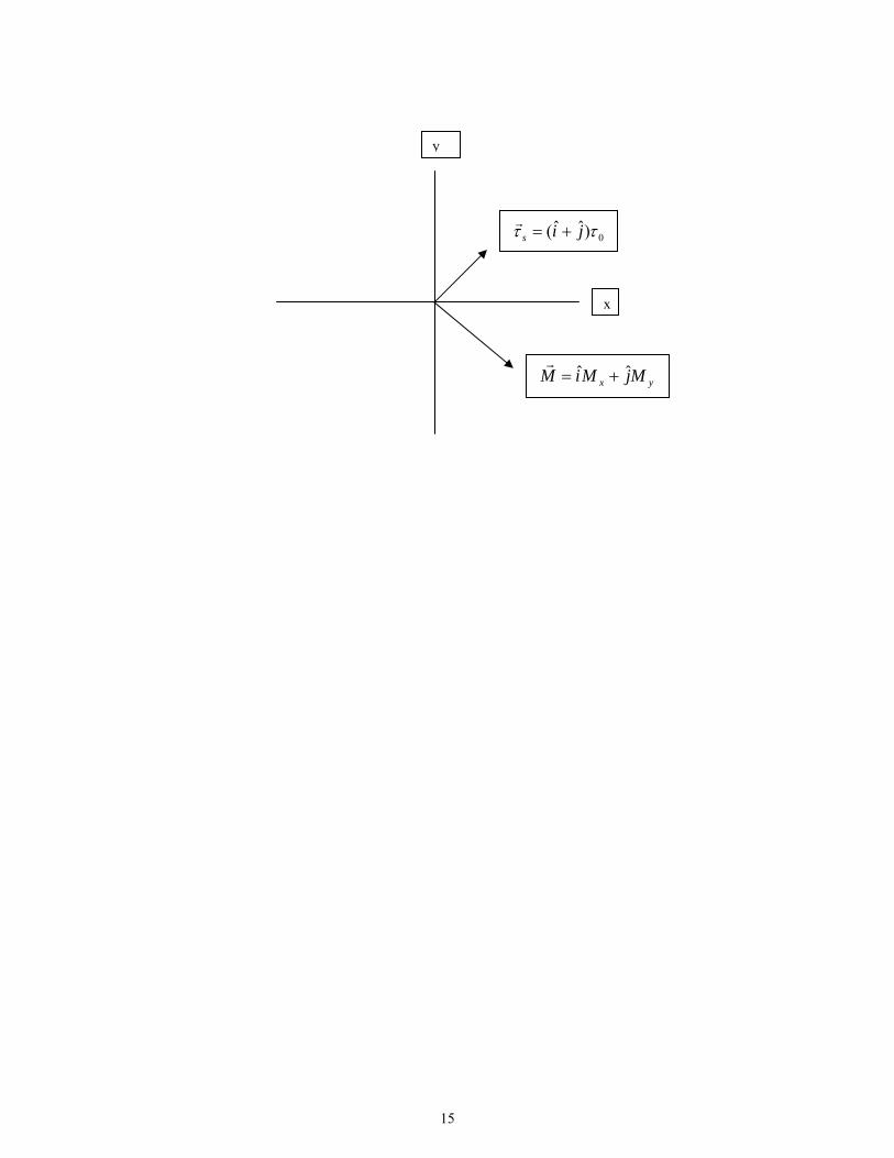
15
yx MjMiM ˆˆ +=r
0)ˆˆ( ττ jis +=r
x
y
Lecture notes on Dynamic Meteorology prepared by Somenath Dutta for old advanced course.
Chapter-V Atmospheric energetics By the term atmospheric energetics, we understand the different forms of energy, the atmosphere possesses and conversion between them. Atmosphere possesses energy mainly in three forms, Viz., the internal energy, the kinetic energy and potential energy. Atmospheric internal energy: It is due to heating of the atmosphere. To obtain an expression for global atmospheric internal energy, let us consider unit mass at temp T0 K. Then internal energy of this unit mass is TCV . Now consider an infinitesimal volume ‘ σd ’ with density ‘ ρ ’ of the atmosphere. This volume is so small that the density ρ practically remains invariant in it. So its mass is σρ d . So, the internal energy of this infinitesimal volume is .σρ dTCV
Hence the internal energy of the global atmosphere is ∫∫∫σ
σρ TdCV = I , say.
Atmospheric potential energy: It is due the vertical position of the centre of gravity of the atmosphere. The potential energy of unit mass at a height ‘z’ above the mean sea level is gz . Hence following the same argument as in I.E, we have the expression for potential energy of global atmosphere as ∫∫∫
σ
σρ dzg = P, say.
Atmospheric kinetic energy: The kinetic energy of the atmosphere is due to different
atmospheric motion. Kinetic energy of an unit mass moving with velocity ‘ vr ’ is .2.vv rr
Hence the expression for kinetic energy for global atmosphere is ∫∫∫σ
σρ dvv2.rv =K, say.
Energy equations: The global internal energy equation is given by
( )∫∫∫∫∫∫ ∇−=σσ
σσρ dvpdQdtdI rr& . ….(1), where,
dtQdQ =& represents the rate of heating.
The above equation tells us that the change in global internal energy is due to net heating/cooling of the atmosphere and due to divergent/convergent motion in the atmosphere. Net heating/ cooling leads to an increase/decrease in temperature, which again leads to an increase/decrease in global I.E. Now to understand how divergence/convergence leads to an increase/decrease in I.E, let us see the following flow charts: Divergence→Expansion→Cooling→Fall in I.E. On the other hand, Convergence→ Compression→Heating→Rise in I.E. The global potential energy equation is given by,
∫∫∫=σ
σρ dwgdtPd ….(2). This equation tells that any change in global potential energy is
due net vertical motion. Net rising/sinking motion leads to an increase/decrease in P.
Lecture notes on Dynamic Meteorology prepared by Somenath Dutta for old advanced course.
The global kinetic energy equation is given by,
( ) ∫∫∫ ∫∫∫∫∫∫∫∫∫ +−∇+∇−=σ σσσ
σρσρσσ dvFwdgdvpdvpdtdK rrrrrr
..).( ….(3)
In the above equation the first term on the right hand side represents the convergence of flux of energy due to work done by/against the pressure force and the last term represents the rate of work by frictional or dissipative forces. Other two terms, viz., the second and third terms have already appeared in the global internal energy equation and in global potential energy equation respectively, but with respective opposite sign. The last term represents the destruction of K.E due to work done against the dissipative forces. Again from Gauss divergence theorem, we know that ∫∫∫∫∫ =∇
Sn dsvpdvp
σ
σ)(. rr, where,
nv is the component of vr normal to the surface ‘ S ’enclosing the volume ‘σ ’. If the global atmosphere is considered to be an isolated closed system, then, 0=nv . So the first term in equation becomes zero. From equation (1) and (3) it follows that for a given sign of ( )∫∫∫ ∇
σ
σdvp rr . global kinetic
energy / global internal energy will be generated at the expense of global internal energy / global kinetic energy. So, this term may be thought of representing the conversion of internal energy to kinetic energy. We denote it by C(I,K). Hence, =),( KIC ( )∫∫∫ ∇
σ
σdvp rr . or =),( IKC ( )∫∫∫ ∇−σ
σdvp rr . .
Already we have seen how divergence or convergence results in decrease or increase in I.E. Also we know that due to divergence or convergence, downstream wind speed increases or decreases, i.e., global K.E increases or decreases. Thus conversion between these two forms of atmospheric energy is due to the divergent flow of the atmosphere. Similarly from equations (2) and (3), it follows that for a given sign of ∫∫∫
σ
σρ dwg
global kinetic energy / global potential energy will be generated at the expense of global potential energy / global kinetic energy. So, this term may be thought of representing the conversion of kinetic energy to potential energy. We denote it by C(K,P). Hence, =),( PKC ∫∫∫
σ
σρ dwg or =),( IKC ∫∫∫−σ
σρ dwg . We have already seen that a
net upward or downward motion leads to an increase or decrease in global P.E. Also a net upward or downward motion causes convergence or divergence, which again leads to decrease or increase in global K.E. Thus conversion between these two forms of atmospheric energy is due to net vertical motion in the atmosphere. Adding equations (1), (2) and (3) we obtain,
∫∫∫ ∫∫∫+=σ σ
σρσρ dvFdQtdEd rr& . ….(4), where, PKIE ++= .
In equation (4), the first term represents the generation of internal energy by net heating of the atmosphere and the second term represents the destruction of K.E due to work done against the dissipative forces. They are respectively denoted by )(IG and )(KD− . Thus equation (4) may be written as
Lecture notes on Dynamic Meteorology prepared by Somenath Dutta for old advanced course.
)()( KDIGtdEd
−= ….(5).
From equation (5) it is clear that for the source of total atmospheric energy, )(IG should be positive and more, i.e., there must be net heating in the atmosphere. Again net heating is by Solar energy. Thus the Sun is source of all atmospheric energy. Now let us consider the kinetic energy equation for horizontal motion. First of all 0=w .
So, we have, ).()( KDKSdt
dK h −= Here, 2. hh
hvv
Krr
= is the kinetic energy for horizontal
motion and ( )∫∫∫ ∇=σ
σdvpKS hrr .)( . Now question which region should be a source for
horizontal kinetic energy. Now in a source region for horizontal kinetic energy there
should be production of horizontal kinetic energy, i.e., .0⟩dt
dK h Again for dt
dKh to be
positive, ( )∫∫∫ ∇=σ
σdvpKS hrr .)( should be positive and large, which requires p to be
high and 0. ⟩∇ hvrr
. This conditions exist in the region of sub-tropical anticyclone which is characterized by high pressure and divergence. Thus the belt of sub-tropical anticyclone is the source for horizontal kinetic energy. Energetics in a hydrostatic and stably stratified atmosphere: By the hydrostatically stable atmosphere we simply understand that there is no net vertical acceleration and by stable stratification we understand that in the atmosphere heavy colder air is below the light warmer air or the potential temperature (θ ) increases with height. Now it will be shown that in such an atmosphere internal energy is proportional to potential energy. This will be established by showing below that any change in I.E causes a similar change in P.E and vice-versa. Increase or decrease in I.E→Increase or decrease in Temperature (T)→Expansion or contraction of an air column of unit cross sectional area→Rising or sinking motion→Increase or decrease in P.E. Similarly, Increase or decrease in P.E→ Rising or Sinking motion→Convergence or divergence→Increase or decrease in I.E. Thus any change in I.E causes a similar change in P.E and vice-versa. Hence internal energy is proportional to potential energy. The above can be established mathematically also as shown below: We consider an air column with unit cross-sectional area. The P.E of this air column is given by
IP
ICRdzTC
CRdzTRdzpzpddpzdzzgP
VV
VPS
∝⇒
===+−=−== ∫∫∫∫ ∫ ∫∞∞∞∞
0000
0 0
0
)( ρρρ
Concept of Available potential energy (APE): We have seen that in a stably stratified and hydrostatically stable atmosphere I.E.
is proportional to the P.E. In such an atmosphere the centre of gravity of the atmosphere is at its lowest elevation. Hence in such condition the atmosphere possesses minimum P.E. and hence it possesses minimum I.E. also. So the sum of these two forms of energy
Lecture notes on Dynamic Meteorology prepared by Somenath Dutta for old advanced course.
will be minimum in a stably stratified and hydrostatically stable atmosphere. Sum of I.E and P.E. is known as total potential energy (TPE).In the reference state, the atmosphere possesses minimum TPE. In such condition the potential temperature(θ) lines are quasi-horizontal, with θ increasing upwards.
But in a part of the globe, the observed state of atmosphere is not necessarily stably stratified and hydrostatically stable. So, the TPE in the observed configuration exceeds that in reference configuration. The excess TPE in the observed configuration makes the atmosphere unstable. In the observed configuration, the θ lines are quasi-vertical instead of quasi-horizontal, keeping warm air, cold air side by side. As a natural tendency the atmosphere in the observed configuration of that part of the globe tends to be stabilized. This requires rising motion of warm air and sinking motion of cold air, i.e., a vertical circulation is required. The necessary kinetic energy to drive this vertical circulation is provided by the excess TPE in the observed configuration over that in reference configuration. This excess TPE in the observed configuration over that in reference configuration is only available for conversion into kinetic energy and is known as available potential energy (APE).
Thus, REFOBS TPETPEAPE −= . It can be shown that, dydxdpPTAPE
sP∫∫ ∫
′∝
0 2
σ, where, σ
is a measure of static stability, P is the mean pressure at any level and 2T ′ is the square of the deviation from mean (areal) temperature at different levels. So, it follows that APE in a barotropic atmosphere is zero. From the above expression of APE, it follows that as the APE over a region increases with the increase in horizontal temperature gradient. So, it’s a measure of baroclinity of the atmosphere over that region.
Lecture notes on Dynamic Meteorology prepared by Somenath Dutta for old advanced course.
Chapter-VI
GLOBAL ANGULAR MOMENTUM BUDGET
Some useful concepts:
Momentum: It is the motion due to combined effect of mass (m) and velocity
( vr ). It is a vector quantity given by vm r . For unit mass momentum is vr .
Angular momentum: It is a vector quantity defined by moment of momentum.
The word ‘moment’ arises in case of rotation only.
Thus if an object of mass (m) and velocity (vr ) rotates about a fixed point or about
an axis (called axis of rotation), then its angular momentum is given by vmr rr× , where, rr
is the position vector of the rotating object. It is a vector quantity.
Now consider a stationary object placed on a circular ring rotating with angular
velocity Ωr
about an axis of rotation. Then, its linear velocity is rrv×Ω
In such case, angular momentum of the object will be )( rr rvr×Ω× = 2rr
rΩ .
Newtons Law:
From the second law of motion we know that
Fdt
vmd rr
=)( , F
rbeing the applied force.
So, Frdt
vmdrrr
rv ×=×
)(
Or, Frdt
vmrd rrrr
×=× )( . LHS is the rate change of angular momentum and RHS is
the torque applied by the force Fr
. Whenever a force Fr
is applied to a body, then a
tendency of rotation about an axis is generated in the body. This tendency of rotation of
the body about that axis is called the torque applied by that force Fr
about that axis.
Thus Newton’s law states that rate of change of angular momentum about an axis
is equal to the torque applied by the forces. Thus if the vector sum of torque is zero, then
angular momentum remains conserved. This is known as conservation of angular
momentum.
Governing equation for global angular momentum budget:
Lecture notes on Dynamic Meteorology prepared by Somenath Dutta for old advanced course.
We consider an unit mass at latitude φ, with zonal velocity u . Then its absolute
zonal angular momentum about the earths axis of rotation is ( ) φϕ coscos aau+Ω = M
(say). To find out an expression for global angular momentum, we consider an
infinitesimal volume, σd with density ρ of the atmosphere. So, the angular momentum
of this infinitesimal volume is σρ dM . Thus the angular momentum of the entire global
atmosphere is given by, ∫∫∫=σ
σρ dMA .
Then the governing equation for global angular momentum budget is given by
∫ ∫ ∫∫ ∫∫ ∫ ∫∞∞∞
+∆−∇−=∂∂
0
2/ 2
0
2/
00
2/ 2
0 000
).(π
φ
ππ
φ
π
φ
π
φλρφφλρ dzddrFddzprdzddVMtA rr
The first term is known as the meridional transport of angular momentum, which
signifies the mechanism of transporting zonal angular momentum in the meridional
direction (N – S).
The second term, which arises due to E-W pressure difference along a latitude
circle, is known as mountain torque term. It is named so, because pressure difference
‘ p∆ ’ is mainly due to the difference of pressure between windward and leeward side of a
section of mountain along that latitude circle.
The third term is known as frictional torque term, and is due to the torque
produced by the frictional force.
Discussion about different terms:
Meridional transport of angular momentum: It can be shown that, this term is
dpvug
adpvg
adpvug
a
sss PPP∫∫∫ ′′+
Ω+=
000 22 cos2cos2cos2 φπφπφπ , where,
∫0cos2
sP
dpvug
a φπ is called the drifting term,
∫Ω 022 cos2
sP
dpvg
a φπ is called the omega transport term and
dpvug
a
sP∫ ′′0cos2 φπ is called the eddy transport term.
Lecture notes on Dynamic Meteorology prepared by Somenath Dutta for old advanced course.
The drifting term signifies the meridional transport of mean zonal angular
momentum across the latitude circle 0φ by the mean meridional circulation.
The omega transport term signifies the meridional transport of zonal angular
momentum, possessed solely due to earths rotation ( φcosaΩ ), by the mean meridional
circulation.
The eddy transport term signifies the meridional transport of eddy zonal
momentum by eddies. For north east-south west oriented westerly troughs, there is less
equator ward transport of eddy zonal angular momentum to its rear and more pole ward
transport of eddy zonal angular momentum ahead of it. So there is a net pole ward
transport of eddy zonal angular momentum for such oriented westerly troughs. Thus NE-
SW oriented westerly troughs transports eddy zonal angular momentum.
Mountain torque term: As already been mentioned p∆ is due to the difference of
pressure between the windward and lee ward side of a mountain barrier.
It is known that, based on the direction of prevailing zonal component, the entire
global atmosphere may be categorized into two regimes, viz., the westerly regime and
easterly regime.
In the westerly regimes wind ward side is to the west of the barrier and the
leeward side is to the east of the barrier. Similarly, in the easterly regimes wind ward side
is to the east of the barrier and the leeward side is to the west of the barrier.
Since p∆ is measured as, WestEast PPp −=∆ , hence as shown in the adjoining figure,
in the westerly regimes, p∆ < 0. Now as the second term is accompanied with a minus (-)
sign, hence the contribution of this term is positive in the westerly regimes and it is
negative in the easterly regimes.
Hence the presence of mountain enhances westerly angular momentum in the
westerly regimes and it reduces that in the easterly regimes.
Frictional torque term: In the easterly regime, frictional force reduces the strength of
easterly wind, that in turn reduces easterly momentum and easterly angular momentum.
This is equivalent to say that in the easterly regime, friction increases the westerly
angular momentum. Hence, there is a net gain in the westerly angular momentum in the
Lecture notes on Dynamic Meteorology prepared by Somenath Dutta for old advanced course.
easterly regimes, due to friction. Following the similar argument it can be said that there
is a net loss in the westerly angular momentum in the westerly regimes, due to friction.
Lecture notes on Dynamic Meteorology for the Advanced Met. training course prepared by Dr.Somenath Dutta.
Hydrodynamic Instability Definition: A mean flow field is said to hydro dynamically unstable if a small perturbation, introduced into the mean flow, grows spontaneously by extracting energy from the mean flow. Classification of hydrodynamic instability: Categorization of hydrodynamic instability may either be based on the state of the mean flow or on the mode of perturbation introduced. Based on the former, hydro dynamic instability may be dynamic or static according as the mean flow is there or not. While discussing Barotropic instability, Baroclinic instability or Inertial instability, we always consider a mean flow having some speed. These are examples of dynamic instabilities. But while discussing Brunt Vaisala instability, we need not to take care of the mean flow. This is example of static instability. Based on the later, hydro dynamic instability may be of two types, viz., parcel instability and wave instability. Some times perturbation may be introduced as a displacement to an air parcel and it is examined under what condition the parcel is moving away from its mean position. This is known as parcel instability. Brunt-Vaisala instability and Inertial instability are examples of parcel instability. In another case, the perturbation is given in the form of a wave super imposed on a mean flow and examined under what conditions the wave is being amplified. This is known as wave instability. Barotropic and Baroclinic instabilities are examples of wave instability. The above categorization is shown below in a tabular form:
Hydrodynamic Instability Based On The State Of Mean Flow Based On The Mode Of Perturbation Static Instability Example: Brunt Vaisala instability.
Dynamic Instability Examples: Inertial, Barotropic, Baroclinic
Parcel Instability Inertial, Brunt Vaisala
Wave Instability Barotropic, Baroclinic
Brunt Vaisala instability: To analyse the Brunt Vaisala instability, we consider an air parcel embedded in a static mean flow. Let the parcel be displaced vertically. If Pρ and Eρ are the densities of air inside the parcel and that of environmental air at new position then the net buoyancy force acting on the air parcel is gV PE )( ρρ − ; where
is the volume of air parcel. Thus considering only the buoyancy force, the vertical momentum equation of the air parcel is V
P
PE
P
PE gV
gVdtdw
ρρρ
ρρρ −
=−
=)(
……(1). Since pressure across the boundary of the
parcel is continuous, it follows that EEPP RTRTP ρρ == ; Where Tp and TE are the temperature of the air parcel and that of environmental air and ‘P’ is the pressure across the boundary of air parcel.
1
Lecture notes on Dynamic Meteorology for the Advanced Met. training course prepared by Dr.Somenath Dutta. Hence it ‘ς ’ denotes the vertical displacement, then we have
E
EP
TTTg
dtd −
=2
2ς ……(2)
Now, ....)0()(0
+⎟⎠⎞
⎜⎝⎛∂∂
+==z
PPP z
TTT ςς
+Γ−= PPT ς)0( …. It is assumed that a dry air parcel follows a dry adiabatic line and a moist air parcel follows a saturated (pseudo) adiabatic line. Hence PΓ is either dry adiabatic lapse rate (DALR) or saturated adiabatic lapse rate (SALR). So we may write aP Γ=Γ ; where, ‘a’ stands for adiabatic, dry or saturated, whatever is applicable. Hence, aPP TT Γ−= ςς )0()( (neglecting higher order terms). Similarly, the environmental temperature at ς=z , is given by,
EEE TT Γ−= ςς )0()( , where, is the environmental lapse rate. EΓSubstituting these expressions of )(ςPT and )(ςET in (2), we obtain
ςς 22
2
Ndtd
−= ……(3), where, E
EP
TgN
Γ−Γ=2 .
The above equation has a stable sine/cosine solution of N2 > 0 and has an unstable exponential solution if N2 <0. Thus the vertical displacement of the parcel is stable if N2 > 0 i.e, if the environmental lapse rate is less then the adiabatic lapse rate other wise unstable if environmental lapse rate exceeds that of parcel. N is known as Brunt Vaisala frequency. Inertial instability: We consider an air parcel embedded in a mean zonally geostrophic flow. Suppose, the air parcel be displaced meridionally from , to 0yy =
yyy δ+= 0 during the period 0tt = and ttt δ+= 0 . Then at the new position, the horizontal equation of motion can be written as,
dtdyffv
dtdu
== ……(4)
gfufuypfu
dtdv
+−=∂∂
−−=ρ1 ….(5).
Integrating (4) between initial and final position we obtain, [ ])()()()( 0000 tyttyftuttu −+=−+ δδ
[ ] yfyyyfyuyyu δδδ =−+=−+⇒ 0000 )()( ……(6) Writing the equation (5) at yyy δ+= 0 , we obtain,
[ ])()( 00 yyuyyufdtdv
g δδ +−+−=
2
Lecture notes on Dynamic Meteorology for the Advanced Met. training course prepared by Dr.Somenath Dutta.
[ ]⎪⎭
⎪⎬⎫
⎪⎩
⎪⎨⎧
⎥⎥⎦
⎤
⎢⎢⎣
⎡+⎟⎟
⎠
⎞⎜⎜⎝
⎛∂
∂+−++−=
=
....)(...)(0
00 yy
uyuyfyuf
yy
gg δδ (Using (6))
At the initial position the air parcel was embedded in the meanflow, which is zonaly geostrophic. Hence, . ( ) )( 00 yuyu g=
Thus at yyy δ+= 0 , ⎟⎟⎠
⎞⎜⎜⎝
⎛∂
∂−−=
yu
fyfdtdv gδ ……(7)
Multiplying both sides of (7) by )( ydtdv δ= and then integrating between initial and final
position, we obtain,
2)( 2yf
dtKd
aδς−=
′…..(8), where, K ′ is the eddy meridional kinetic energy of the parcel
and aς is the absolute vorticity of the mean flow. Since the RHS of (8), represents the rotational K.E of the mean flow, it appears that perturbation grows by extracting rotational K.E of the mean flow. In the northern hemisphere f > 0. Thus the K.E of the parcel will increase with time if
0<aς , i.e., if the mean flow has absolute anticyclonic vorticity and will decrease if 0>aς , i.e., if the mean flow has absolute cyclonic vorticity and neutral if 0=aς .
In the southern hemisphere, f < 0. Thus the K.E of the parcel will increase with time if 0>aς , which corresponds to absolute anticyclonic vorticity in the southern hemisphere
and will decrease if 0<aς , which again corresponds to absolute cyclonic vorticity in the southern hemisphere and neutral if 0=aς . Thus, a mean flow with cyclonic vorticity is inertially stable and with anticyclonic vorticity is inertially unstable. The result may be interpreted as follows: A mean flow with a cyclonic absolute vorticity is itself active enough so that it cannot spare its energy to grow perturbation in it, where as that with an anticyclonic absolute vorticity is not active enough, so that it can spare its energy to the perturbation to grow. Barotropic Instability: Definition: A zonal mean flow field is said to be barotropically unstable if a small perturbation, introduced in it, grows spontaneously by extracting kinetic energy from the mean flow. Barotropic instability analysis: To, analyse the barotropic instability; we start with the non divergent barotropic model. The governing equation for this is given by
βςςςς vy
vx
ufVt
−⎟⎟⎠
⎞⎜⎜⎝
⎛∂∂
+∂∂
−=+∇−=∂∂ )(.
rr……(1)
3
Lecture notes on Dynamic Meteorology for the Advanced Met. training course prepared by Dr.Somenath Dutta. We apply have perturbation technique, following which we split the fields into basic and perturbation parts as below:
),,()( tyxuyuu ′+= ),,(0 tyxvv ′+=
Hence, ςςς +′=−∂′∂
−∂′∂
=∂∂
−∂∂
=dyud
yu
xv
yu
xv
Substituting in the above governing equation, we obtain,
⎟⎟⎠
⎞⎜⎜⎝
⎛−′−
∂′∂
−=∂′∂
2
2
dyudv
xu
tβςς ……(2)
Here, we introduce, perturbation stream function, ),,( tyxψ ′ , such that,
xv
∂′∂
=′ψ and
yu
∂′∂
−=′ψ , so that, ψς ′∇=′ 2
Hence (2) reduces to,
02
22 =⎟⎟
⎠
⎞⎜⎜⎝
⎛−
∂′∂
+′∇⎟⎠⎞
⎜⎝⎛
∂∂
+∂∂
dyud
xxu
tβψψ …..(3)
We seek the wave solution for (3) like
)()(),,( tkxieyAtyx νψ −=′ …..(4) Subject to the boundary condition
0)( =±dA ……(5) Substituting (4) in (3) we have ( )( ) ( ) 02 =−++−+− uikAuikiAAk &&&& βν …..(6) Multiplying both sides of (6) by *A , the complex conjugate of A, we obtain
( ) ( ) ( ) 022*
22 =−++−⎥⎥⎦
⎤
⎢⎢⎣
⎡−+− uAkku
dydA
dyAAdAk &&&
βν ……(7)
Integrating the above with respect to ‘ ’ betweeny dy ±= , we obtain
( )dyucu
Ady
dydAAk
d
d
d
d∫∫+
−
+
−
−−
=⎪⎭
⎪⎬⎫
⎪⎩
⎪⎨⎧
+ &&β)(
2222 …….(8)
Now, , where, and are respectively the real and imaginary part of the phase velocity So,
ir iccc += rc ic'.'c ( ) ir iccucu −−=− . Multiplying the numerator and denominator
of the integrand on RHS of (8) by the complex conjugate of )( cu − , we obtain,
4
Lecture notes on Dynamic Meteorology for the Advanced Met. training course prepared by Dr.Somenath Dutta.
( )[ ][ ] ( )dyu
ccuiccuA
dydydAAk
d
d ir
ird
d∫∫+
−
+
−
−+−
+−=
⎪⎭
⎪⎬⎫
⎪⎩
⎪⎨⎧
+ &&β22
2222
)(
L.H.S of the above equation is a pure real number, hence the R.H.S has to be so, which requires
( )( )
022 =+−
−∫+
−
dyccu
ucd
d iri
&&β . Since, ,0≠ic hence, ( )( )
022 =+−
−∫+
−
dyccu
ud
d ir
&&β …..(9).
Since the denominator of the integrand in (9) is a positive definite quantity, hence, it is always positive, Thus the above definite integral to vanish, ( )u&&−β mush change sign within the limit of integration. This further requires that there must exist some point, say
, between , such that cyy = dy ±= ( ) 0=− = cyyu&&β ……(10). This is the necessary condition for barotropic instability. Thus for a mean zonal flow to be barotropically unstable, the necessary condition is that at same intermediate latitude the mean flow has an extreme absolute vorticity. Energetics of barotropic instability: To study the energetics of barotropic instability, first we will show that in the non-divergent barotropic model the mean kinetic energy remains conserved. For that we start with non divergent vorticity equation,
βςςςς vy
vx
ufVt
−⎟⎟⎠
⎞⎜⎜⎝
⎛∂∂
+∂∂
−=+∇−=∂∂ )(.
rr
0. 2 =∂∂
+∇⎟⎠⎞
⎜⎝⎛ ∇+∂∂
xV
tψβψ
rr
0.. =∂∂
+∇⎟⎠⎞
⎜⎝⎛ ∇+∂∂
∇x
Vt
ψβψrrrr
Multiplying above by ''ψ , we obtain,
0.. =∂∂
+∇⎟⎠⎞
⎜⎝⎛ ∇+∂∂
∇x
Vt
ψβψψψrrrr
02
....
2
=∂
⎟⎠⎞
⎜⎝⎛∂
+∇⎟⎠⎞
⎜⎝⎛ ∇+∂∂
∇−⎥⎦
⎤⎢⎣
⎡∇⎟⎠⎞
⎜⎝⎛ ∇+∂∂
∇x
Vt
Vt
ψ
βψψψψrrrrrrrr
Integrating the above over a volume ''σ , consisting of from dy −= to , from bottom to top of the atmosphere and over an entire wavelength of a barotropic wave, we obtain,
dy =
0=dtdK , where, ∇+
∂∂
≡rr
.Vtdt
d and σψψ
σ
dK ∫∫∫∇∇
=2.rr
.
Now, if KKK ′+= , then we have,
dtKd
dtKd
−=′
. Thus, the barotropic instability grows by extracting K.E from the mean
flow.
5
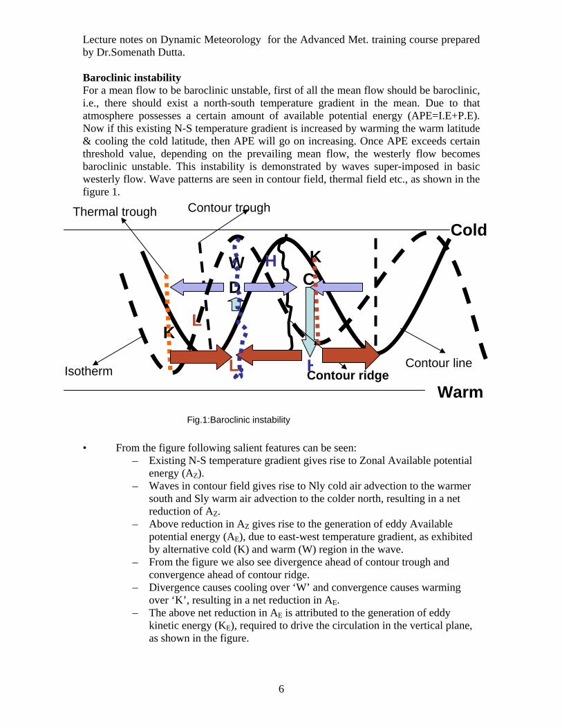
Lecture notes on Dynamic Meteorology for the Advanced Met. training course prepared by Dr.Somenath Dutta. Baroclinic instability For a mean flow to be baroclinic unstable, first of all the mean flow should be baroclinic, i.e., there should exist a north-south temperature gradient in the mean. Due to that atmosphere possesses a certain amount of available potential energy (APE=I.E+P.E). Now if this existing N-S temperature gradient is increased by warming the warm latitude & cooling the cold latitude, then APE will go on increasing. Once APE exceeds certain threshold value, depending on the prevailing mean flow, the westerly flow becomes baroclinic unstable. This instability is demonstrated by waves super-imposed in basic westerly flow. Wave patterns are seen in contour field, thermal field etc., as shown in the figure 1.
• From the figure following salient features can be seen:
– Existing N-S temperature gradient gives rise to Zonal Available potential energy (AZ).
– Waves in contour field gives rise to Nly cold air advection to the warmer south and Sly warm air advection to the colder north, resulting in a net reduction of AZ.
– Above reduction in AZ gives rise to the generation of eddy Available potential energy (AE), due to east-west temperature gradient, as exhibited by alternative cold (K) and warm (W) region in the wave.
– From the figure we also see divergence ahead of contour trough and convergence ahead of contour ridge.
– Divergence causes cooling over ‘W’ and convergence causes warming over ‘K’, resulting in a net reduction in AE.
– The above net reduction in AE is attributed to the generation of eddy kinetic energy (KE), required to drive the circulation in the vertical plane, as shown in the figure.
D C
L
H
K
W K
Contour lineIsotherm
Contour troughThermal trough Cold
Warm Contour ridge L H
Fig.1:Baroclinic instability
6
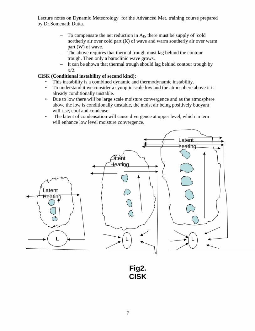
Lecture notes on Dynamic Meteorology for the Advanced Met. training course prepared by Dr.Somenath Dutta.
– To compensate the net reduction in AE, there must be supply of cold northerly air over cold part (K) of wave and warm southerly air over warm part (W) of wave.
– The above requires that thermal trough must lag behind the contour trough. Then only a baroclinic wave grows.
– It can be shown that thermal trough should lag behind contour trough by π/2.
CISK (Conditional instability of second kind): • This instability is a combined dynamic and thermodynamic instability. • To understand it we consider a synoptic scale low and the atmosphere above it is
already conditionally unstable. • Due to low there will be large scale moisture convergence and as the atmosphere
above the low is conditionally unstable, the moist air being positively buoyant will rise, cool and condense.
• The latent of condensation will cause divergence at upper level, which in tern will enhance low level moisture convergence.
L
Latent Heating
L
Latent Heating
L
Latent heating
Fig2. CISK
7
Lecture notes on Dynamic Meteorology for the Advanced Met. training course prepared by Dr.Somenath Dutta.
• The enhanced low level moisture convergence in tern will again enhance heating. • Thus there is a co-operative mutual interaction between large scale moisture
convergence and cumulus scale heating. • The above gives rise to a different type of instability, known as CISK. • The above has been explained schematically in fig.2.
8
Related Documents