Submitted to Management Science manuscript (Please, provide the manuscript number!) Authors are encouraged to submit new papers to INFORMS journals by means of a style file template, which includes the journal title. However, use of a template does not certify that the paper has been accepted for publication in the named jour- nal. INFORMS journal templates are for the exclusive purpose of submitting to an INFORMS journal and should not be used to distribute the papers in print or online or to submit the papers to another publication. Dynamic Inventory Repositioning in On-Demand Rental Networks Saif Benjaafar Department of Industrial and Systems Engineering, University of Minnesota, [email protected] Daniel Jiang Department of Industrial Engineering, University of Pittsburgh, [email protected] Xiang Li Target Corporation, [email protected] Xiaobo Li Department of Industrial Systems Engineering and Management, National University of Singapore, [email protected] We consider a rental service with a fixed number of rental units distributed across multiple locations. The units are accessed by customers without prior reservation and on an on-demand basis. Customers can decide on how long to keep a unit and where to return it. Because of the randomness in demand and in returns, there is a need to periodically reposition inventory away from some locations and into others. In deciding on how much inventory to reposition and where, the system manager balances potential lost sales with repositioning costs. Although the problem is increasingly common in applications involving on-demand rental services, not much is known about the nature of the optimal policy for systems with a general network structure or about effective approaches to solving the problem. In this paper, first, we show that the optimal policy in each period can be described in terms of a well-specified region over the state space. Within this region, it is optimal not to reposition any inventory, while, outside the region, it is optimal to reposition but only such that the system moves to a new state that is on the boundary of the no-repositioning region. We also provide a simple check for when a state is in the no-repositioning region. Second, we leverage the features of the optimal policy, along with properties of the optimal cost function, to propose a provably convergent approximate dynamic programming algorithm to tackle problems with a large number of dimensions. Key words : rental networks; inventory repositioning; optimal policies, approximate dynamic programming algorithms, stochastic dual dynamic programming 1. Introduction We consider a rental service with a fixed number of rental units distributed across multiple loca- tions. Customers are able to rent a unit for one or more periods without a prior reservation and 1 Electronic copy available at: https://ssrn.com/abstract=2942921

Welcome message from author
This document is posted to help you gain knowledge. Please leave a comment to let me know what you think about it! Share it to your friends and learn new things together.
Transcript

Submitted to Management Sciencemanuscript (Please, provide the manuscript number!)
Authors are encouraged to submit new papers to INFORMS journals by means ofa style file template, which includes the journal title. However, use of a templatedoes not certify that the paper has been accepted for publication in the named jour-nal. INFORMS journal templates are for the exclusive purpose of submitting to anINFORMS journal and should not be used to distribute the papers in print or onlineor to submit the papers to another publication.
Dynamic Inventory Repositioning in On-DemandRental Networks
Saif BenjaafarDepartment of Industrial and Systems Engineering, University of Minnesota, [email protected]
Daniel JiangDepartment of Industrial Engineering, University of Pittsburgh, [email protected]
Xiang LiTarget Corporation, [email protected]
Xiaobo LiDepartment of Industrial Systems Engineering and Management, National University of Singapore, [email protected]
We consider a rental service with a fixed number of rental units distributed across multiple locations. The
units are accessed by customers without prior reservation and on an on-demand basis. Customers can decide
on how long to keep a unit and where to return it. Because of the randomness in demand and in returns, there
is a need to periodically reposition inventory away from some locations and into others. In deciding on how
much inventory to reposition and where, the system manager balances potential lost sales with repositioning
costs. Although the problem is increasingly common in applications involving on-demand rental services,
not much is known about the nature of the optimal policy for systems with a general network structure or
about effective approaches to solving the problem. In this paper, first, we show that the optimal policy in
each period can be described in terms of a well-specified region over the state space. Within this region,
it is optimal not to reposition any inventory, while, outside the region, it is optimal to reposition but only
such that the system moves to a new state that is on the boundary of the no-repositioning region. We also
provide a simple check for when a state is in the no-repositioning region. Second, we leverage the features
of the optimal policy, along with properties of the optimal cost function, to propose a provably convergent
approximate dynamic programming algorithm to tackle problems with a large number of dimensions.
Key words : rental networks; inventory repositioning; optimal policies, approximate dynamic programming
algorithms, stochastic dual dynamic programming
1. Introduction
We consider a rental service with a fixed number of rental units distributed across multiple loca-
tions. Customers are able to rent a unit for one or more periods without a prior reservation and
1
Electronic copy available at: https://ssrn.com/abstract=2942921

Benjaafar, Jiang, Li, and Li: Dynamic Inventory Repositioning2 Article submitted to Management Science; manuscript no. (Please, provide the manuscript number!)
without specifying, at the time of initiating the rental, the duration of the rental or the return
location. That is, customers are allowed to return a unit rented at one location to any other loca-
tion, We refer to such a service as being on-demand and one-way. Demand that cannot be fulfilled
at the location at which it arises is considered lost and incurs a lost sales penalty (or is fulfilled
through other means at an additional cost). Because of the randomness in demand, the length of
the rental periods, and return locations, there is a need to periodically reposition inventory away
from some locations and into others. Inventory repositioning is costly and the cost depends on both
the origin and destination of the repositioning. The service provider is interested in minimizing the
lost revenue from unfulfilled demand (lost sales) and the cost incurred from repositioning inventory
(repositioning cost). Note that more aggressive inventory repositioning can reduce lost sales but
leads to higher repositioning cost. Hence, the firm must carefully mitigate the trade-off between
demand fulfillment and inventory repositioning.
Problems with the above features are increasingly common in applications involving on-demand
rental services1. We are particularly motivated by a variety of one-way car sharing services that
allow customers to rent from one location and return to another location. Examples include the
car sharing service ShareNow (a merger of formerly Car2Go and DriveNow) and similar recently
launched services such as LimePod, BlueLA, and BlueSG. These services are on-demand in the
sense that they do not require an ahead-of-time reservation or the specification of a return duration
ahead of use. They are one-way in the sense that customers are not required to return a vehicle
to the same location from which it was rented and instead are allowed to decide on a location,
among those in the network, that is most convenient. In other words, these services let customers
decide on when and where to return a vehicle, with this information not necessarily shared with
the rental service until the rental terminates. For example, LimePod advertises its service as being
free-floating, offering customers the ability to walk up to any parked vehicle, initiate a rental via
its mobile app, and then return the vehicle to any legal parking location within the service region
at any time. Customers are charged based on the duration of the rental, with charges calculated
at the time the rental terminates.
A challenge in managing these services (and other examples of on-demand rental systems) is the
spatial mismatch between vehicle supply and demand that arises from the uncertainty in rental
origins, duration, and destinations.Unless adequately mitigated with the periodic repositioning of
inventory, the spatial mismatch between supply and demand can lead to a significant loss in revenue.
1 Renting may become even more prevalent as the economy shifts away from a model built on the exclusive ownershipof resources to one based on on-demand access and resource sharing (Sundararajan 2016) (Benjaafar and Hu 2019).
Electronic copy available at: https://ssrn.com/abstract=2942921

Benjaafar, Jiang, Li, and Li: Dynamic Inventory RepositioningArticle submitted to Management Science; manuscript no. (Please, provide the manuscript number!) 3
Although the problem is increasingly common in applications involving on-demand rental ser-
vices2, not much is known about the nature of the optimal policy for systems with a general network
structure or about effective approaches to solving the problem. This lack of results appears to
be due to the multidimensional nature of the problem (i.e., more than one inventory location),
compounded by the presence of randomness in demand, rental periods, and return locations, as
well as lost sales. In this paper, we address these limitations through two main contributions. The
first contribution is theoretical and the second is computational:
• On the theoretical side, we offer a characterization of the optimal policy for the dynamic
inventory repositioning problem in a general network setting, accounting for randomness in trip
volumes, duration, origin, and destination as well as spatial and temporal dependencies (e.g.,
likelihood of a trip terminating somewhere being dependent on its origin as well as trip volumes
that are dependent on time and location).
• On the computational side, we describe a new cutting-plane-based approximate dynamic pro-
gramming (ADP) algorithm that can effectively solve the dynamic repositioning problem to near-
optimality. We provide a proof of convergence for our algorithm that takes a fundamentally different
view from existing cutting-plane-based approaches (this can be viewed as a theoretical contribu-
tion to the ADP literature, independent from the repositioning application). We also propose a
clustering-based extension to our ADP method that scales to large-scale systems and illustrate its
effectiveness on problems with up to 100 locations.
Specifically, we formulate the repositioning problem as a multi-period stochastic dynamic pro-
gram. We show that the optimal policy in each period can be described in terms of two well-specified
regions over the state space. If the system is in a state that falls within one region, it is optimal not
to reposition any inventory (we refer to this region as “the no-repositioning” region). If the system
is in a state that is outside this region, then it is optimal to reposition some inventory but only
such that the system moves to a new state that is on the boundary of the no-repositioning region.
Moreover, we provide a simple check for when a state is in the no-repositioning region, which also
allows us to compute the optimal policy more efficiently.
One of the distinctive features of the problem considered lies in its non-linear state update func-
tion. This non-linearity introduces difficulties in showing the convexity of the problem that must be
solved in each period. To address this difficulty, we leverage the fact that the state update function
2 Other applications where the periodic repositioning of inventory is important include bike share systems wherecustomers can pick up a bike from one location and return it to any other location within the service region; shippingcontainer rentals in the freight industry where containers can be rented in one location and returned to a differentlocation, with locations corresponding in some cases to ports in different countries; and the use of certain medicalequipment, such as IV pumps and wheelchairs, in large hospitals by different departments located in various areas ofthe hospital.
Electronic copy available at: https://ssrn.com/abstract=2942921

Benjaafar, Jiang, Li, and Li: Dynamic Inventory Repositioning4 Article submitted to Management Science; manuscript no. (Please, provide the manuscript number!)
is piecewise-affine and derive properties for the directional derivatives of the value function. This
approach has potential applicability to other systems with piecewise-affine state update functions.
Due to the curse of dimensionality, the optimal policy (and the value function) can be difficult
to compute for problems with more than a small number of dimensions. To address this issue, we
leverage the results obtained regarding the structure of both the value function and the optimal
policy to construct an approximate dynamic programming algorithm. The algorithm combines
aspects of approximate value iteration (see, for example, De Farias and Van Roy (2000) and Munos
and Szepesvari (2008)) and stochastic dual dynamic programming (see Pereira and Pinto (1991)).
We conduct numerical experiments to illustrate the effectiveness of jointly utilizing value function
and policy structure, which, to our knowledge, has not yet been explored by related methods in
the literature.
The rest of the paper is organized as follows. In Section 2, we review related literature. In Section
3, we describe and formulate the problem. In Sections 4 and 5, we give our structural results for
the optimal value function and the optimal policy, respectively. Next, in Section 6 we describe
our ADP approach, along with several numerical studies. In Section 7, we address the problem of
scaling the ADP algorithm to large systems via the clustering-based extension. In Section 8, we
provide concluding comments.
Notation. Throughout the paper, the following notation will be used. We use e to denote
a vector of all ones, ei to denote a vector of zeros except 1 at the ith entry, and 0 to denote
a vector of all zeros (the dimension of these vectors will be clear from the context). Also, we
write ∆n−1(M) to denote the (n−1)-dimensional simplex, i.e., ∆n−1(M) = (x1, . . . , xn) |∑n
i=1 xi =
M,x≥ 0. Similarly, we use Sn(M) to denote the n-dimensional simplex with interior, i.e., Sn(M) =
(x1, . . . , xn) |∑n
i=1 xi ≤ M,x ≥ 0. Throughout, we use ordinary lowercase letters (e.g., x) to
denote scalars, and boldfaced lowercase letters (e.g., x) to denote vectors. The Euclidean norm is
denoted ‖ · ‖2. For functions f1 and f2 with domain X , let ‖f1‖∞ = supx∈X |f1(x)| and let f1 ≤ f2
denote f1(x)≤ f2(x) for all x ∈ X . We denote the boundary of a set E by B(E), and the interior
of E by E.
2. Literature Review
There is growing literature on inventory repositioning in car and bike sharing systems; see for
example Nair and Miller-Hooks (2011), Shu et al. (2013), Bruglieri et al. (2014), O’Mahony and
Shmoys (2015), Freund et al. (2016), Liu et al. (2016), Ghosh et al. (2017), Schuijbroek et al. (2017),
Li et al. (2018), Shui and Szeto (2018), Nyotta et al. (2019), and the references therein. Most of
this literature focuses on the static repositioning problem, where the goal is to find the optimal
placement of vehicles before demand arises, with no more repositioning being made afterwards (e.g.,
Electronic copy available at: https://ssrn.com/abstract=2942921

Benjaafar, Jiang, Li, and Li: Dynamic Inventory RepositioningArticle submitted to Management Science; manuscript no. (Please, provide the manuscript number!) 5
repositioning overnight for the next day). The objective function in the associated optimization
problem typically accounts for repositioning and user dissatisfaction costs (e.g., lost sales). Much
of this work employs mixed integer programming formulations and focuses on the development
of algorithms and heuristics. Similarly, the papers that focus on dynamic repositioning generally
consider heuristic solution techniques and do not offer structural results regarding the optimal
policy (see, for example, Ghosh et al. (2017) and Li et al. (2018)).
A notable exception is Li and Tao (2010) who study a finite horizon problem with two locations.
They show that the optimal policy in the last period is characterized by a two-limit control policy
(a single dimensional version of the policy we show is true in general). They conjecture that the
optimal policy has a similar structure in other periods but do not provide a proof. In this paper,
we prove that this conjecture is indeed true. Moreover, we prove that a generalized version of the
policy holds for problems with more than two locations.
A related stream of literature models vehicle sharing systems as closed queueing networks; see,
for example, George and Xia (2011), Waserhole and Jost (2016), Banerjee et al. (2017), Braverman
et al. (2019), Banerjee et al. (2018) and Benjaafar et al. (2021). This literature treats time as
being continuous with demand (in the form of an arrival process) that is typically stationary. A
common objective in this literature is to identify control policies that maximize a function of the
amount of demand satisfied. Control levers include demand throttling (e.g., via pricing), vehicle
dispatching (deciding on how to allocate available vehicles to demand as it arises), and empty vehi-
cle repositioning. In general, optimal dynamic policies, such as the ones we consider in this paper,
are difficult to characterize. Instead much of this literature relies on analyzing asymptotic regimes,
when either the number of vehicles goes to infinity or both the number of vehicles and demand go
to infinity. Braverman et al. (2019) consider the optimal repositioning problem in the asymptotic
regime where both demand and number of vehicles are allowed to go to infinity. The resulting static
repositioning policy is shown to provide an upper bound on the optimal objective function for the
finite problem. The static repositioning problem is also discussed in Benjaafar et al. (2021) under
a demand balance assumption and using an approximation for vehicle availability at each location.
Waserhole and Jost (2016) and Banerjee et al. (2017) consider the optimal pricing problem in
the asymptotic regime when the number of vehicles goes to infinity. The resulting static pricing
policy is shown to provide guaranteed bounds for the finite system. Banerjee et al. (2018) consider
the optimal dispatching problem for a stylized setting under the infinite number of vehicles regime
and show that the resulting policy provides strong performance bounds.
In this paper, we take a different approach by studying optimal dynamic policies which are
generally state-dependent. We consider a setting where time is discretized and allow for demand to
be non-stationary. However, we do treat the inventory of vehicles as continuous (this is also the case
Electronic copy available at: https://ssrn.com/abstract=2942921

Benjaafar, Jiang, Li, and Li: Dynamic Inventory Repositioning6 Article submitted to Management Science; manuscript no. (Please, provide the manuscript number!)
under the asymptotic regimes considered in the queueing-based literature). We suspect, though we
do not prove it, that the optimal dynamic policy for vehicle repositioning under a queueing model
may share similar features to the optimal policy we show for our setting.
Other related papers include Chung et al. (2018) who analyze incentive-based repositioning
policies for bike sharing, and Bimpikis et al. (2019) and Balseiro et al. (2020) who consider the
spatial aspect of pricing in ride-sharing networks, a related problem to ours, and Ma et al. (2020)
who consider a setting with full information to design a spatial-temporal mechanism for prices
and wages with desirable properties. Other work considers strategic issues such as fleet sizing,
service region design, infrastructure planning, and user dissatisfaction; see, for example, Jian et al.
(2016), Raviv and Kolka (2013), He et al. (2017), Lu et al. (2017), Freund et al. (2017), Kabra
et al. (2020), and Kaspi et al. (2017). Comprehensive reviews of the literature on vehicle and bike
sharing can be found in He et al. (2019) and Freund et al. (2019).
There is literature that addresses inventory repositioning that arises in other settings, including
in the context of repositioning of empty containers in the shipping industry, empty railcars in
railroad operations, cars in traditional car rentals, and emergency vehicles; see, for example, Lee
and Meng (2015) for a comprehensive review. The literature on empty container repositioning is
particularly extensive. However that literature focuses on simple networks and relies on heuristics
when considering more general problems; see for example Song (2005) and Li et al. (2007). To our
knowledge, there are no results regarding the optimal policy for a general network. There is also
extensive literature on emergency vehicle repositioning when the demand from different locations
is random. Berman (1981) introduces a dynamic programming formulation of the problem. More
recent work includes Maxwell et al. (2010) who describe an ADP approach and Maxwell et al.
(2014) who provide a lower bound on the performance of repositioning policies; see Belanger et al.
(2019) for a comprehensive review of this literature.
The paper that is closest to ours is He et al. (2020), which was subsequent to an earlier version of
this paper3 and which considers a problem similar to ours and solves it using a robust optimization
approach. Further discussion of this paper can be found in Section 4. Another subsequent paper
that is similar to both our work and He et al. (2020) is Zhao et al. (2020): they derive a structural
result for the special case of two locations, two periods, and no ongoing rentals when there is a
fixed cost to repositioning. Zhao et al. (2020) build upon the models first introduced in our paper4
and the work of He et al. (2020).
3 The first version of our paper appeared online ahead of the first version of He et al. (2020). He et al. (2020) refer tothat version of our paper.
4 Zhao et al. (2020) cite the working version of this paper.
Electronic copy available at: https://ssrn.com/abstract=2942921

Benjaafar, Jiang, Li, and Li: Dynamic Inventory RepositioningArticle submitted to Management Science; manuscript no. (Please, provide the manuscript number!) 7
The problem we consider in this paper shares features with the well-studied dynamic portfo-
lio optimization problem when there are transaction costs. The dynamic portfolio optimization
problem involves periodically reallocating funds among different assets, taking into account the
stochastic nature of how the value of these assets evolves over time. Constantinides (1979) shows
that the structure of the optimal policy resembles that of the optimal policy we describe in this
paper for the vehicle sharing problem; see also Leland (1999). That is, it is optimal to do noth-
ing if the system state (defined by the current values of the assets) is within a specified region;
otherwise, it is optimal to reallocate funds so that the system state after reallocation lies on the
boundary of the do-nothing region. Eberly and Van Mieghem (1997) consider a broader class of
resource/capacity allocation problems and prove a similar structure for the optimal policy; see
Van Mieghem (2003) for a review of related literature. A discussion of computational approaches,
bounds on the optimal solution, and heuristics can be found in Muthuraman and Kumar (2006)
and Brown and Smith (2011) and the references therein. The dynamics of the problem we consider
are different (e.g., the amount of demand at one location in one period affects the distribution
of vehicles at other locations in future periods). Moreover, in our case, the total capacity in the
system must be held constant. Our problem is neither a special case nor a generalization of the
dynamic portfolio optimization problem. However, these similarities hint that both problems may
belong to a more general class of problems whose optimal solution has such a feature.
Finally, there is related literature on computational methods that can solve problems with convex
value functions. Some well-known cutting-plane-based approaches are the stochastic decomposition
algorithm of Higle and Sen (1991), the stochastic dual dynamic programming (SDDP) method
introduced in Pereira and Pinto (1991), and the cutting plane and partial sampling approach of
Chen and Powell (1999). Our method is most closely related to SDDP, where full expectations are
computed at each iteration. Linowsky and Philpott (2005), Philpott and Guan (2008), Shapiro
(2011), and Girardeau et al. (2014) provide convergence analyses of SDDP, but these analyses
are designed for finite-horizon problems (or two-stage stochastic programs) and rely on an exact
terminal value function and/or that there only exist a finite number of cuts.
Our algorithm is most closely related to the cutting plane methods for the infinite horizon setting
proposed in Birge and Zhao (2007) and Warrington et al. (2019). Birge and Zhao (2007) proves
uniform convergence of the value function approximations to optimal value for the case of linear
dynamics, given a strong condition that the cut in each iteration is computed at a state where a
Bellman error criterion is approximately maximized. Computation of such a state is a difference
of convex functions optimization problem (or a suitable approximation). Warrington et al. (2019)
focus on the deterministic setting, use a fixed set of sampled states at which cuts are computed,
and do not show consistency of their algorithm. Our algorithm removes these restrictions, yet we
Electronic copy available at: https://ssrn.com/abstract=2942921

Benjaafar, Jiang, Li, and Li: Dynamic Inventory Repositioning8 Article submitted to Management Science; manuscript no. (Please, provide the manuscript number!)
are still able to show uniform convergence to the optimal value function. In particular, our analysis
allows for non-linear dynamics and cuts to be computed at states sampled from a distribution.
Furthermore, our use of policy structure (i.e., the no-repositioning region characterization) in an
SDDP-like algorithm is new.
As an alternative to cutting plane algorithms, Godfrey and Powell (2001) and Powell et al. (2004)
propose methods based on stochastic approximation (see Kushner and Yin (2003)) to estimate
scalar or separable convex functions, where a piecewise-linear approximation is updated iteratively
via noisy samples while ensuring that convexity is maintained. Nascimento and Powell (2009)
extend the technique to a finite-horizon ADP setting for the problem of lagged asset acquisition
(single inventory state) and provides a convergence analysis; see also Nascimento and Powell (2010).
However, these methods are not immediately applicable to our situation, where the value function
is multi-dimensional.
3. Problem Formulation
We consider a product rental network consisting of n locations and N rental units. Inventory
levels are reviewed periodically and, in each period, a decision is made on how much inventory
to reposition away from one location to another. Inventory repositioning is costly and the cost
depends on both the origins and destinations of the repositioning. The review periods are of equal
length and decisions are made over a specified planning horizon, either finite or infinite.
Demand in each period is positive and random, with each unit of demand requiring the usage
of one rental unit for one or more periods, with the rental period being also random. Demand
that cannot be satisfied at the location at which it arises is considered lost and incurs a lost sales
penalty. A location in the context of a free-floating car sharing system may correspond to a specified
geographic area (e.g., a zip code area, a neighborhood, or a set of city blocks). Units rented at
one location can be returned to another. Hence, not only are rental durations random but so are
return destinations. At any time, a rental unit can be either at one of the locations, available for
rent, or in an “ongoing rental” state with a customer.
The sequence of events in each period is as follows. At the beginning of the period, inventory
level at each location is observed. A decision is then made on how much inventory to reposition
away from one location to another. Subsequently, demand is realized at each location followed by
the realization of product returns. Our model assumes, for tractability, that repositioning occurs
within a single review period5. Note that the solution we obtain is still implementable (feasible)
even if the assumption regarding the repositioning time does not hold.
5 Similar assumptions on relocation/travel times have been made in much of the existing literature on this topic. Heet al. (2020) assume that both customer trips and repositioning trips can be completed within a period. Balseiro et al.(2020) and Waserhole and Jost (2016) assume that travel times are instantaneous. Bimpikis et al. (2019) assumesthat going from one location to another takes one period.
Electronic copy available at: https://ssrn.com/abstract=2942921

Benjaafar, Jiang, Li, and Li: Dynamic Inventory RepositioningArticle submitted to Management Science; manuscript no. (Please, provide the manuscript number!) 9
We index the periods by t ∈ N, with t = 1 indicating the first period in the planning horizon.
We let xt = (xt,1, . . . , xt,n)∈Rn denote the vector of inventory levels before repositioning in period
t, where xt,i denotes the corresponding inventory level at location i. Our model uses continuous
inventory levels for tractability. This means that the resulting repositioning decisions produced by
the model will be continuous. To implement them in a discrete system, one would need to perform
a rounding step6. Similarly, we let yt = (yt,1, . . . , yt,n) ∈ Rn denote the vector of inventory levels
after repositioning in period t, where yt,i denotes the corresponding inventory level at location i.
Note that inventory repositioning should always preserve the total on-hand inventory. Therefore,
we require∑n
i=1 yt,i =∑n
i=1 xt,i. As we will make clear later, xt is only a part of the state in our
dynamic system. The second part of the state is the vector of ongoing rentals, defined below.
Inventory repositioning is costly and, for each unit of inventory repositioned away from location
i to location j, a cost of cij is incurred. Consistent with our motivating application of a car sharing
system, we assume there is a cost associated with the repositioning of each unit; see He et al.
(2020) for similar treatment. Let c= (cij) denote the cost matrix and let wij denote the amount of
inventory to be repositioned away from location i to location j. Then, the minimum cost associated
with repositioning from an inventory level x to another inventory level y is given by the solution
to the following linear program:
min c ·w
subject ton∑
i=1
wij −n∑
k=1
wjk = yj −xj ∀ j = 1, . . . , n
w≥ 0.
The first constraint ensures that the change in inventory level at each location is consistent with
the amounts of inventory being moved into (∑
iwij) and out of (∑
kwjk) that location. The second
constraint ensures that the amount of inventory being repositioned away from one location to
another is always nonnegative so that the associated cost is accounted for in the objective. It is
clear that the value of the linear program depends only on z = y−x. Define
C(z) = min c ·w
subject ton∑
i=1
wij −n∑
k=1
wjk = zj ∀ j = 1, . . . , n
w≥ 0,
(1)
for any z ∈H where H := z ∈Rn :∑n
i=1 zi = 0 . Then the inventory repositioning cost from x to
y is C(y − x). Without loss of generality, we assume that cij ≥ 0 satisfy the triangle inequality
(i.e., cik ≤ cij + cjk for all i, j, k).
6 This is reasonable when the number of rental units N is large and is consistent with treatment elsewhere in theliterature (see for example He et al. (2020), Li and Tao (2010), and Zhao et al. (2020)) and in much of the literatureon stochastic inventory control (see for example Zipkin (2000)).
Electronic copy available at: https://ssrn.com/abstract=2942921

Benjaafar, Jiang, Li, and Li: Dynamic Inventory Repositioning10 Article submitted to Management Science; manuscript no. (Please, provide the manuscript number!)
We let dt = (dt,1, . . . , dt,n) denote the vector of random demands in period t, with dt,i corre-
sponding to the demand at location i. The amount of demand that cannot be fulfilled is given by
(dt,i− yt,i)+ = max(0, dt,i− yt,i). Let βi denote the per unit lost sales penalty incurred in location
i. Then, the total lost sales penalty incurred in period t across all locations is given by L(yt,dt) =∑n
i=1 βi(dt,i − yt,i)+. We assume that each product can be rented at most once within a review
period, that is, rental periods are longer than review periods.
To model the randomness in the rental return process, we assume that, at the end of each
period t, a random fraction pt,ij of products rented from location i is returned to location j for all
i, j ∈ 1,2, . . . , n, with the rest continuing to be rented. We let P t denote the matrix of random
fractions, i.e.,
P t =
pt,11 · · · pt,1n
.... . .
...pt,n1 · · · pt,nn
.
The ith row of P t must satisfy∑n
j=1 pt,ij ≤ 1. The case where∑n
j=1 pt,ij < 1 corresponds to a
setting where rentals are not immediately returned, while the case where∑n
j=1 pt,ij = 1 corresponds
to a setting where rental periods are exactly equal to one. Let µt denote the joint distribution of
dt and P t, i= 1,2, . . . , n. We assume that the random sequence (dt,P t) is independent over time,
and the expected aggregate demand in each period is finite (i.e.,∫∞
0
∑n
i=1 dt,i dµt <+∞). However,
we allow dt and P t to be dependent. The randomness of P t is consistent with the on-demand
nature of many rental services, where the provider does not have information regarding the return
destination.
Finally, let γt,i for i = 1,2, . . . , n and t = 1,2, . . . , T denote the quantity of the product rented
from location i that remains outstanding at the beginning of period t. Let ρ∈ [0,1) be the rate at
which future costs are discounted.
The model we described above can be formulated as a Markov decision process. Fix a time
period t. The system states correspond to the on-hand inventory levels xt and the outstanding
inventory levels γt. The state space is specified by the (2n−1)-dimensional simplex, i.e., (xt,γt)∈∆2n−1(N). Throughout the paper, we denote S := Sn(N) and ∆ := ∆2n−1(N) since these notations
are frequently used. Actions correspond to the vector of target inventory levels yt. Given state
(xt,γt), the action space is an (n− 1)-dimensional simplex, i.e., yt ∈∆n−1(eTxt). The transition
probabilities are induced by the state update function:
xt+1,i = (yt,i− dt,i)+ +∑n
j=1(γt,j + min(yt,j, dt,j))pt,ji ∀ i= 1,2, . . . , n, t= 1,2, . . . , Tγt+1,i = (γt,i + min(yt,i, dt,i))(1−
∑n
j=1 pt,ij) ∀ i= 1,2, . . . , n, t= 1,2, . . . , T.
Given a state (xt,γt) and an action yt, the repositioning cost is given by C(yt − xt), and the
expected lost sales penalty is given by lt(yt) =∫Lt(yt,dt)dµt =
∫ ∑i βi(dt,i−yt,i)+ dµt. The single-
period cost is the sum of the inventory repositioning cost and lost sales penalty rt(xt,γt,yt) =
Electronic copy available at: https://ssrn.com/abstract=2942921

Benjaafar, Jiang, Li, and Li: Dynamic Inventory RepositioningArticle submitted to Management Science; manuscript no. (Please, provide the manuscript number!) 11
C(yt − xt) + lt(yt). The objective is to minimize the expected discounted cost over a specified
planning horizon. In the case of a finite planning horizon with T periods, the optimality equations
are given by
vt(xt,γt) = minyt∈∆n−1(eTxt)
rt(xt,γt,yt) + ρ
∫vt+1(xt+1,γt+1)dµt (2)
for t= 1,2, . . . , T , and vT+1(xT+1,γT+1) = 0 where ρ is the discount factor introduced above.
It is useful to note that the problem to be solved in each period can be expressed in the following
form:
vt(xt,γt) = minyt∈∆n−1(eTxt)
C(yt−xt) +ut(yt,γt), (3)
where
ut(yt,γt) =
∫Ut(yt,γt,dt,P t)dµt, (4)
and
Ut(yt,γt,dt,P t) =Lt(yt,dt) + ρvt+1(τx(yt,γt,dt,P t), τγ(yt,γt,dt,P t)), (5)
where
τx(y,γ,d,P ) = (y−d)+ +P T (γ+ min(y,d)), τγ(y,γ,d,P ) = (γ+ min(y,d)) (e−P te), (6)
where denotes the Hadamard product (or the entrywise product), i.e., (a1, a2, . . . , an) (b1, b2, . . . , bn) = (a1b1, a2b2, . . . , anbn). The next two assumptions state some useful conditions on
the return fractions P t and the repositioning costs cij.
Assumption 1. Let pmin ∈ (0,1] be a constant. For every period t, there exists a random variable
pt ∈ [pmin,1] such that∑n
j=1 pt,ij =∑n
j=1 pt,kj = pt, ∀ i, k = 1,2, . . . , n. An equivalent statement is
that pt,ij = pt qt,ij for some qt,ij where∑n
j=1 qt,ij = 1 for all i.
Assumption 1 implies that the probability of a vehicle being returned in a given period does not
depend on the location at which the vehicle is rented, but the distribution of the return locations
does depend on the origin7
Assumption 2. The repositioning costs satisfy ρcmax− cmin ≤ pmin (βi− cmin) for all i= 1, . . . , n,
where cmax = maxi,j cij and cmin = mini,j; i 6=j cij.
7 We make this assumption for tractability of the theoretical analysis in Section 4, but note that it is plausible becausewhether to return and where to return are usually two separate decisions for customers. Furthermore, in the case ofrental networks located in dense urban regions, we expect many rental locations to have similar properties in termsof customers’ rental/return behaviors. In Appendix A.1 we provide empirical support for this assumption based onreal data obtained from the one-way car sharing service Car2Go.
Electronic copy available at: https://ssrn.com/abstract=2942921
Benjaafar, Jiang, Li, and Li: Dynamic Inventory Repositioning12 Article submitted to Management Science; manuscript no. (Please, provide the manuscript number!)
The second assumption enforces boundedness in the difference of cost parameters, with the upper
bound depending on pmin. If pmin = 1, where the rental duration is always one period (corresponding
to the setting of He et al. (2020)), the restriction reduces to ρcmax ≤ βi for all i. This means that
the cost of lost sales outweighs the cost of inventory repositioning in the next period8. If pmin < 1,
the assumption prevents the unpleasant situation where one might want to deliberately “hide”
the inventory due to the difference in the repositioning cost. It is clear from the assumption that
ρcmax− cmin ≤ pmin(βi− cmin)≤ pt (βi− cmin) for all i.
Under Assumptions 1 and 2, we are able to show (see Section 4 and 5) that the value function in
each period, consisting of the lost sales and the cost-to-go as defined next, is always convex, which
is perhaps surprising given the non-linear state update and the lost sales feature.
4. Convexity of ut(yt,γt)
The main purpose of this section is to establish the convexity of ut(yt,γt) defined in (5) for all
periods t. We will also show that a similar result holds for the infinite-horizon case. These results
will allow us later on (see Section 5) to characterize the structure of the optimal policy. They will
also be useful in developing an efficient solution procedure (see Section 6).
4.1. The Finite-Horizon Problem
In this section, we consider the finite-horizon problem discussed in section 3. For the last period
(period T ), uT (yT ,γT ) = lT (yT ) is clearly convex. A natural question is whether the convexity of
ut(·) is preserved when we consider previous periods. The main difficulty is that the state update
in (6) is non-linear. However, if we introduce an auxiliary variable ω= mind,y, the state update
function could be written in the following linear form:
τx(y,γ,d,P ) = y−ω+P T (γ+ω), τγ(y,γ,d,P ) = (γ+ω) (e−P te).
We show that we can replace the constraint ω= mind,y with ω≤mind,y, which would then
imply the convexity of ut(·) (see Appendix A.3 for the analysis, given as a series of technical
lemmas). Let
u′(x,γ;z,η) = limt↓0
u(x+ tz,γ+ tη)−u(x,γ)
t(7)
denote the directional derivative of u(·) at (x,γ) along the direction (z,η). We call (z,η) a feasible
direction at (x,γ) if (x+ tz,γ+ tη)∈∆ for small enough t > 0. The main results are summarized
in the following theorem.
8 A similar but slightly weaker condition is assumed in He et al. (2020). In this sense, the convexity in our paper caninclude their results as a special case except that in their model, lost sales costs depend on both origin and destinationand the return destinations are known by the platform at the time of rental. In our case, we assume, consistent withthe reality of many one-way vehicle sharing systems, that the destination of a rental is not revealed until a realizedtrip is completed. In settings where the lost sales cost depends on both the origin and destination of a trip, βi hasthe interpretation of the expected lost sales cost over all destinations.
Electronic copy available at: https://ssrn.com/abstract=2942921

Benjaafar, Jiang, Li, and Li: Dynamic Inventory RepositioningArticle submitted to Management Science; manuscript no. (Please, provide the manuscript number!) 13
Theorem 1. Suppose Assumptions 1 and 2 hold. For t= 1, . . . , T , both ut(·) defined in (4) and
vt(·) defined in (2) are convex and continuous in ∆. Moreover, the following properties of ut(yt,γt)
hold for t= 1, . . . , T :
(a) ut(yt,γt) = Edt,P t [Ut(yt,γt,dt,P t)] where Ut(yt,γt,dt,P t) can be reformulated as the fol-
lowing convex optimization program
Ut(yt,γt,dt,P t) = minω,xt+1,γt+1
∑n
i=1 βi(dt,i−ωi) + ρvt+1(xt+1,γt+1)
subject to xt+1 = yt−ω+P Tt (γt +ω),
γt+1 = (γt +ω) (e−P te),ω≤ yt, andω≤ dt;
(8)
(b) |u′t(yt,γt;±η,∓η)| ≤∑n
i=1 βiηi for all (yt,γt)∈∆ and any feasible direction (±η,∓η) with
η≥ 0;
(c) u′t(yt,γt;0,z)≤ (ρ/2)cmax
∑n
i=1 |zi| for all (x,γ) ∈∆ and any feasible direction (0,z) with
eTz = 0;
(d) ut(·) is Lipschitz continuous on ∆ with Lipschitz constant (3/2)√
2nβmax, where βmax =
maxi βi.
A comprehensive proof of Theorem 1 can be found in Appendix A.3. Here, we give an outline
of the approach. We apply induction, starting from vT+1(y,γ) = 0. We show in Proposition 3 and
Proposition 4 that if vt+1(·) is convex and satisfies certain bounds on its directional derivatives,
then for any realization of dt,P t, the function Ut(yt,γt,dt,P t) can be reformulated as the convex
program (8) and satisfies two types of bounds on its directional derivatives. The first type (item 1)
shows that if we turn some of the available inventory into ongoing rentals, the reduced or enlarged
cost can be upper bounded by the lost sales cost of these products. The same bound holds if we
remove some of the ongoing rentals and make them available at the locations from which they
were rented. The second type bound states that if we change the origin of some of the ongoing
rentals (i.e., we change γ only), the difference in cost can be upper bounded by the product of
(ρcmax/2) and the one-norm of the difference in γ. The primary reason is that the total return
fraction for period t, pt, does not depend on the origin. Therefore, the difference of costs is at
most the repositioning cost in the next period. To complete the induction, we show in Proposition
5 that given the convexity of ut(yt,γt) and aforementioned bounds on its directional derivatives,
vt(xt,γt) is convex and satisfies the directional derivative bounds required by Proposition 3 and 4.
Finally, we show that item (b) and (c) imply item (d).
We note that although the formulation in (8) has similarities to the result in Lemma 1 in He
et al. (2020), our proof technique is fundamentally different. First, to show that the reformulation
is exact, we need to show that if ω 6= min(dt,yt), we can increase some components of ω so that the
Electronic copy available at: https://ssrn.com/abstract=2942921
Benjaafar, Jiang, Li, and Li: Dynamic Inventory Repositioning14 Article submitted to Management Science; manuscript no. (Please, provide the manuscript number!)
objective function is not worse while keeping it feasible. For the problem in He et al. (2020) (which
corresponds to our problem with pmin = 1), since all the outstanding cars are be returned at the end
of the period, we can arrive at any state xt+1 by adjusting the decision variable yt. However, when
pmin < 1, a change in ω would result in a change in γt+1, which can not be rebalanced by changing
yt. To show the monotonicity of ω, we need the directional derivative of vt+1(·) to satisfy delicate
bounds as required in Proposition 3. Second, though the aforementioned bound of vt+1(·) is clearly
true for the last period, for general t, we require that the directional derivatives of ut(·) satisfy the
two types of bounds in Theorem 1. To show that these bounds indeed hold, we carry out careful
convex analysis and induction per Proposition 3, Proposition 4 and Proposition 5. Above all, it is
highly non-trivial to show the exactness of the reformulation in (8). Our proof technique might be
of independent interest for high-dimensional inventory problems with lost sales.
An immediate consequence of the reformulation is that, if all random variables satisfy discrete
distributions, the problem can be written as a large-scale linear program.
Corollary 1. Suppose Assumptions 1 and 2 hold and (dt,P t) follows a discrete distribution
for all t, then the optimal policy π∗ = (π∗1 , . . . , π∗T ) can be computed as the optimal solution to a
large-scale linear program.
Corollary 1 allows us to approximate the optimal policy by replacing each expectation with the
finite sum of a few samples and solve the large-scale LP. However, since the size of the LP grows
exponentially in the number of samples and the number of periods, for reasonable values of T , we
can only afford to solve the problem with a single sample path. In Section 6, we use one sample
(the mean demand) for each period to approximate the optimal policy and compare it with our
ADP solution procedure.
4.2. The Infinite-Horizon Problem
We have shown that ut(·) is convex for each period for the finite-horizon problem. Next we show
that the same can be said about the stationary problem with infinitely many periods. In such a
problem, we denote the common distribution for (dt,P t) by µ. Similarly, we denote the common
values of Lt(·), lt(·) and rt(·) by L(·), l(·) and r(·), respectively. We use π to denote a stationary
policy that uses the same decision rule π in each period. Under π, the state of the process is a
Markov random sequence (Xt,Γt), t= 1,2, . . .. The optimization problem can be written as a
Markov decision process (MDP):
v(x,γ) = minπ
Eπx
∞∑
t=1
ρt−1r(Xt,Γt, π(Xt,Γt))
, (9)
where X1 = x a.e. is the initial state of the process. Let vT (x,γ) =
minπ Eπx∑T
t=1 ρt−1r(Xt,Γt, πt(Xt,Γt))
denote the value function of a stationary problem with
Electronic copy available at: https://ssrn.com/abstract=2942921

Benjaafar, Jiang, Li, and Li: Dynamic Inventory RepositioningArticle submitted to Management Science; manuscript no. (Please, provide the manuscript number!) 15
T periods. It is well known that the functions vT (·) converge uniformly to v(·) and v(·) is the
unique solution to
v(x,γ) = miny∈∆n−1(eTx)
r(x,γ,y) + ρ
∫v(τx(y,γ,d,P ), τγ(y,γ,d,P ))dµ, (10)
where τx(·) and τγ(·) correspond to the state update functions defined in (6), i.e.,
τx(y,γ,d,P ) = (y−d)+ +P T (γ+ min(y,d)) ∀ t= 1,2, . . . , T, andτγ(y,γ,d,P ) = (γ+ min(y,d)) (e−P te) ∀ t= 1,2, . . . , T.
(11)
For details, the reader may refer to Chapter 6 of Puterman (1994).
As in the finite-horizon version, the problem to be solved can be written in the following form:
v(x,γ) = miny∈∆n−1(eTx)
C(y−x) +u(y,γ), (12)
where
u(y,γ) =
∫U(y,γ,d,P )dµ, (13)
and
U(y,γ,d,P ) =L(y,d) + ρv(τx(y,γ,d,P ), τγ(y,γ,d,P )). (14)
Theorem 2. Suppose Assumptions 1 and 2 hold. Both u(·) defined in (13) and v(·) defined in
(12) are convex and continuous in ∆. Moreover, we have:
(a) U(y,γ,d,P ) defined in (14) can be reformulated as the following convex optimization pro-
gramU(y,γ,d,P ) = minω,τx,τγ
∑n
i=1 βi(di−ωi) + ρv(τx,τγ)
subject to τx = y−ω+P T (γ+ω),τγ = (γ+ω) (e−Pe),ω≤ y,andω≤ d;
(15)
(b) |u′(y,γ;∓η,±η)| ≤∑n
i=1 βiηi for all (x,γ) ∈ ∆ and any feasible direction (∓η,±η) with
η≥ 0;
(c) u′(y,γ;0,z) ≤ (ρcmax/2)∑n
i=1 |zi| for all (x,γ) ∈ ∆ and any feasible direction (0,z) with
eTz = 0; and
(d) u(·) is Lipschitz continuous on ∆ with Lipschitz constant (3/2)√
2nβmax, where βmax =
maxi βi.
5. The Optimal Repositioning Policy
In this section, we characterize the structure of the optimal policy. We do so for both the finite
and infinite horizon cases. Recall that, for both cases the repositioning problem can be stated as
v(x,γ) = miny∈∆n−1(eTx)
C(y−x) +u(y,γ) for (x,γ)∈∆, (16)
Electronic copy available at: https://ssrn.com/abstract=2942921

Benjaafar, Jiang, Li, and Li: Dynamic Inventory Repositioning16 Article submitted to Management Science; manuscript no. (Please, provide the manuscript number!)
where C(·) is the repositioning cost specified by (1) and u(·) is a convex and continuous function
that maps ∆ to R ∪ −∞,∞. The principle result of this section is the characterization of the
optimal policy through the no-repositioning set, the collection of inventory levels from which no
repositioning should be made. The no-repositioning set for a function u(·) when the outstanding
inventory level is γ can be defined as follows:
Ωu(γ) = x∈∆n−1(I) : u(x,γ)≤C(y−x) +u(y,γ) ∀ y ∈∆n−1(I) ,∀γ ∈ S (17)
where I =N −∑n
i=1 γi. Note that I is a function of γ (or equivalently x). For notational simplicity,
we suppress the dependency of I on γ (or x). By definition, no repositioning should be made
from inventory levels inside Ωu(γ). In the following theorem, we show that Ωu(γ) is non-empty,
connected and compact and, for inventory levels outside Ωu(γ), it is optimal to reposition to some
point on the boundary of Ωu(γ). Recall that we denote the boundary of a set E by B(E), and the
interior of E by E.
Theorem 3. The no-repositioning set Ωu(γ) is nonempty, connected and compact for all γ ∈ S.
An optimal policy π∗ to (16) satisfies
π∗(x,γ) =x if x∈Ωu(γ);π∗(x,γ)∈B(Ωu(γ)) otherwise.
(18)
Solving a nondifferentiable convex program such as (16) usually involves some computational effort.
One way to reduce this effort, suggested by Theorem 3, is to characterize the no-repositioning
set Ωu(γ). Characterizing the no-repositioning region can help us identify when a state is inside
Ωu(γ), which allows our ADP algorithm to more easily compute the value iteration step; see
Section 6. Recall that u′(x,γ;z,η) = limt↓0u(x+tz,γ+tη)−u(x,γ)
tdenotes the directional derivative
of u(·) at (x,γ) along the direction (z,η). Since u(·) is assumed to be convex and continuous in ∆,
u′(x,γ;z,η) is well defined for (x,γ) ∈∆. Recall also that (z,η) is a feasible direction at (x,γ)
if (x+ tz,γ + tη) ∈∆ for small enough t > 0. In what follows, we provide a series of first order
characterizations of Ωu(γ), the first of which relies on the directional derivatives.
Proposition 1. x∈Ωu(γ) if and only if
u′(x,γ;z,0)≥−C(z) (19)
for any feasible direction (z,0) at (x,γ).
Proposition 1 is essential for several subsequent results. However, using Proposition 1 to verify
whether a point lies inside the no-repositioning set is computationally impractical, as it involves
checking an infinite number of inequalities in the form of (19). In the following proposition, we pro-
vide a second characterization of Ωu(γ) using the subdifferentials. Before we proceed, we introduce
Electronic copy available at: https://ssrn.com/abstract=2942921

Benjaafar, Jiang, Li, and Li: Dynamic Inventory RepositioningArticle submitted to Management Science; manuscript no. (Please, provide the manuscript number!) 17
the following notations. g is said to be a subgradient of u(·,γ) at x if u(y,γ)≥ u(x,γ)+gT (y−x)
for all y. The set of all subgradients of u(·,γ) at x is denoted by ∂xu(x,γ). It is well known that
∂xu(x,γ) is nonempty, closed and convex for x in the interior, which is equivalent to x> 0 in our
setting.
Proposition 2. x ∈ Ωu(γ) if ∂xu(x,γ)∩ G 6= ∅, where G = (g1, . . . , gn) : gi − gj ≤ cij ∀ i, j. If
x> 0, then the converse is also true.
Proposition 2 suggests whether a point lies inside the no-repositioning set depends on whether
u(·,γ) has certain subgradients at this point. Such a characterization is useful if we can compute
the subdifferential ∂xu(x,γ). In particular, if u(·,γ) is differentiable at x, then ∂xu(x,γ) consists
of a single point ∇xu(x,γ). In this case, determining its optimality only involves checking n(n−1)
inequalities.
Corollary 2. Suppose u(·,γ) is differentiable at x ∈∆n−1(I). Then, x ∈Ωu(γ) if and only if∂u(x,γ)
∂xi− ∂u(x,γ)
∂xj≤ cij for all i, j.
The no-repositioning set Ωu(γ) can take on many forms. We first discuss the case where there
are only two locations. In this case, the no-repositioning set corresponds to a closed line segment
with the boundary being the two end points. The optimal policy reduces to a state-dependent
two-threshold policy.
Corollary 3. Suppose n = 2. For γ ∈ S, let I = N − γ1 − γ2. Then Ωu(γ) = (x, I − x) : x ∈[s1(γ), s2(γ)], where s1(γ) = infx : u′((x, I − x,γ1, γ2); (1,−1,0,0)) ≥ −c21 and s2(γ) = supx :
−u′((x, I −x,γ1, γ2); (−1,1,0,0))≤ c12. An optimal policy π∗ to (16) satisfies
π∗(x, I −x,γ1, γ2) = (s1(γ), I − s1(γ)) if x< s1(γ),π∗(x, I −x,γ1, γ2) = (x, I −x) if s1(γ)≤ x< s2(γ),π∗(x, I −x,γ1, γ2) = (s2(γ), I − s2(γ)) otherwise.
Corollary 3 is a direct consequence of Theorem 3, Proposition 1, and the fact that there are only
two feasible directions. It shows that the optimal policy to problem (16) in the two-dimensional
case is described by two thresholds s1(γ)< s2(γ) on the on-hand inventory level x at location 1.
If x is lower than s1, it is optimal to bring the inventory level up to s1 by repositioning inventory
from location 2 to location 1. On the other hand, if x is greater than s2, it is optimal to bring
the inventory level at location 1 down to s2. When x falls between s1 and s2, it is optimal not to
reposition as the benefit of inventory repositioning cannot offset the cost.
When there are more than two locations, a threshold policy is not naturally defined due to
the total inventory constraint. In what follows, we characterize the no-repositioning set for two
important special cases, the first of which corresponds to when u(·,γ) is a convex quadratic function.
Electronic copy available at: https://ssrn.com/abstract=2942921
Benjaafar, Jiang, Li, and Li: Dynamic Inventory Repositioning18 Article submitted to Management Science; manuscript no. (Please, provide the manuscript number!)
If the demands are uniformly distributed, then for the last period, u(·,γ) is a quadratic function
since only the lost sales cost is involved. In this case, the no-repositioning set is a polyhedron
defined by n(n− 1) linear inequalities.
Example 1. For a fixed γ, suppose u(y,γ) = yTB(γ)y + yTb(γ) + b0(γ) and B(γ) is posi-
tive semidefinite. By Corollary 2, Ωu(γ) = y ∈∆n−1(I) : 2yTBi(γ) + bi(γ)− 2yTBj(γ)− bj(γ)≤cij ∀ i, j, where Bi(γ) is the i-th row of B(γ).
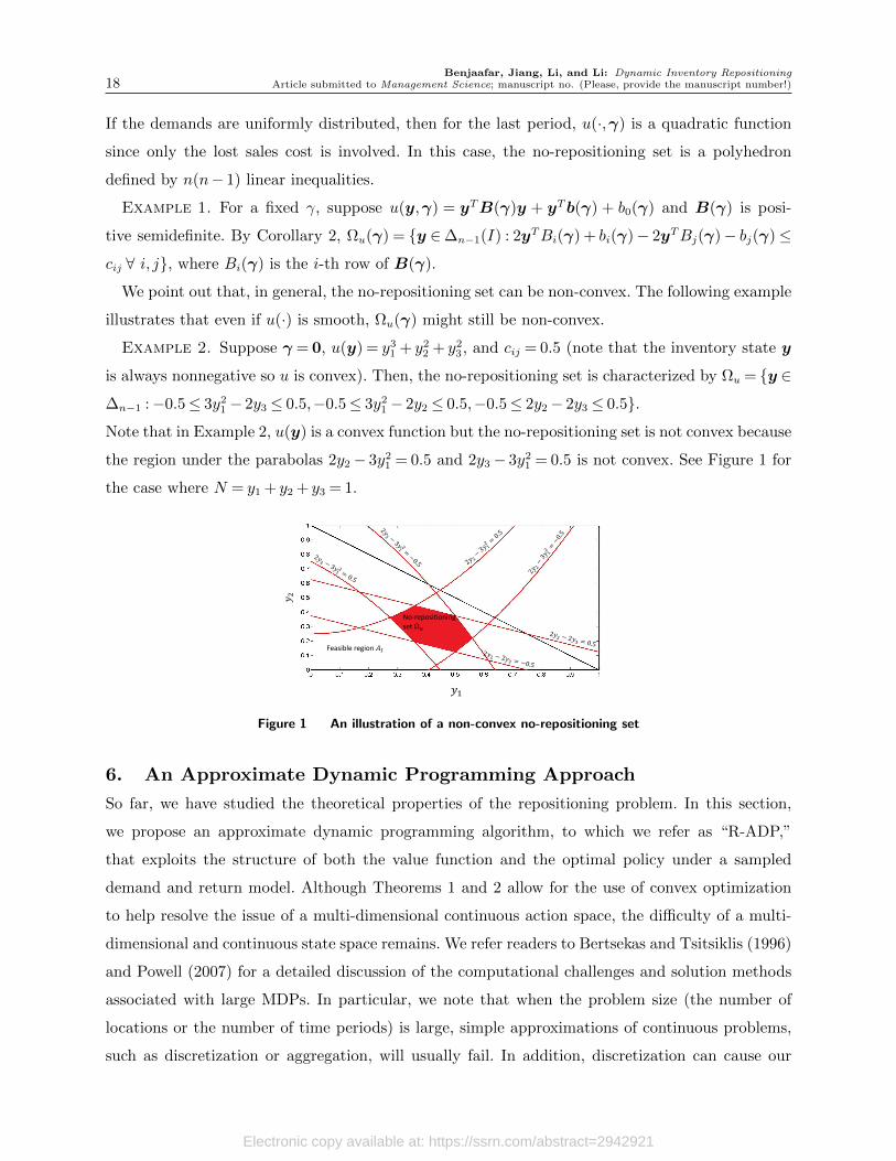
We point out that, in general, the no-repositioning set can be non-convex. The following example
illustrates that even if u(·) is smooth, Ωu(γ) might still be non-convex.
Example 2. Suppose γ = 0, u(y) = y31 + y2
2 + y23, and cij = 0.5 (note that the inventory state y
is always nonnegative so u is convex). Then, the no-repositioning set is characterized by Ωu = y ∈∆n−1 :−0.5≤ 3y2
1 − 2y3 ≤ 0.5,−0.5≤ 3y21 − 2y2 ≤ 0.5,−0.5≤ 2y2− 2y3 ≤ 0.5.
Note that in Example 2, u(y) is a convex function but the no-repositioning set is not convex because
the region under the parabolas 2y2− 3y21 = 0.5 and 2y3− 3y2
1 = 0.5 is not convex. See Figure 1 for
the case where N = y1 + y2 + y3 = 1.
𝑦1
Feasible region 𝐴𝐼
No-repositioning set Ω𝑢
Figure 1 An illustration of a non-convex no-repositioning set
6. An Approximate Dynamic Programming Approach
So far, we have studied the theoretical properties of the repositioning problem. In this section,
we propose an approximate dynamic programming algorithm, to which we refer as “R-ADP,”
that exploits the structure of both the value function and the optimal policy under a sampled
demand and return model. Although Theorems 1 and 2 allow for the use of convex optimization
to help resolve the issue of a multi-dimensional continuous action space, the difficulty of a multi-
dimensional and continuous state space remains. We refer readers to Bertsekas and Tsitsiklis (1996)
and Powell (2007) for a detailed discussion of the computational challenges and solution methods
associated with large MDPs. In particular, we note that when the problem size (the number of
locations or the number of time periods) is large, simple approximations of continuous problems,
such as discretization or aggregation, will usually fail. In addition, discretization can cause our
Electronic copy available at: https://ssrn.com/abstract=2942921

Benjaafar, Jiang, Li, and Li: Dynamic Inventory RepositioningArticle submitted to Management Science; manuscript no. (Please, provide the manuscript number!) 19
structural properties to break down, which means the convexity result and characterization of
the optimal policy given Theorems 1 and 2 can no longer be readily used. Informal numerical
experiments show that even if we do not consider the ongoing rentals (rental period is always one),
approximating the dynamic program via discretization within a reasonable accuracy is already a
formidable task for a three-location problem.
It is thus necessary for us to consider more scalable techniques. A key feature of the algorithm
we describe next is that each iteration involves solving one or more linear programs, allowing
it to leverage the scalability and computational advantages of off-the-shelf solvers. We show via
numerical experiments that the algorithm can produce high quality solutions on problems with
states up to 19 dimensions (10 locations) within a reasonable amount of time. The algorithm also
possesses the important theoretical property of asymptotically optimal value function approxima-
tions; see Theorem 4. In the rest of this section, we motivate and describe the algorithm, prove its
convergence, discuss some practical considerations, and present the numerical results.
6.1. The R-ADP Algorithm
Theorems 1 and 2 describe the most important feature of our dynamic program, that u(·), the
summation of current period lost sales and the cost-to-go, is convex and continuous. Moreover,
Proposition 2 provides a characterization of when it is optimal not to reposition. Our algorithm
takes advantage of these two structural results. It is well known that a convex function can be
written as the point-wise supremum of its tangent hyperplanes, i.e.,
u(y,γ) = supy,γ
u(y, γ) + (y− y)T∇yu(y, γ) + (γ− γ)T∇γu(y, γ).
This suggests that we can build an approximation to u(·) by iteratively adding lower-bounding
hyperplanes, with the hope that the approximation becomes arbitrarily good when enough hyper-
planes are considered. This is the main idea of the algorithm, with special considerations made to
account for the complicated structure of the state update functions. Using a lower, piecewise-affine
approximation of a convex function is a commonly-used idea in stochastic programming; see, for
example, Figure 1 of Philpott and Guan (2008) for an illustration.
Our algorithm is motivated by various aspects of approximate value iteration (see De Farias and
Van Roy (2000) and Munos and Szepesvari (2008)) and stochastic dual dynamic programming (see
Pereira and Pinto (1991)). The features and analysis that distinguish our ADP algorithm from
previous work in the literature are summarized below.
1. Our algorithm has the ability to skip the optimization step when a sampled state is detected
as being in the no-repositioning region. This step uses Proposition 2 and it is applied to the value
function approximation at every iteration.
Electronic copy available at: https://ssrn.com/abstract=2942921

Benjaafar, Jiang, Li, and Li: Dynamic Inventory Repositioning20 Article submitted to Management Science; manuscript no. (Please, provide the manuscript number!)
2. The underlying model of SDDP and other cutting-plane methods (see, e.g., Higle and Sen
(1991), Pereira and Pinto (1991), Birge and Zhao (2007)) is typically a two-stage or multi-stage
stochastic linear program. In our case, we have non-linear state updates, which makes the opti-
mization step of the algorithm difficult. To sidestep this difficulty, in our algorithm, we approximate
u(·) instead of v(·), while computing the state updates outside of the optimization step.
3. Our algorithm is designed for the infinite horizon setting, where each approximation “boot-
straps” from the previous approximation and convergence is achieved despite the absence of a
terminal condition such as “vT+1 ≡ 0” used in the finite-horizon case. As such, the convergence
analyses used in Chen and Powell (1999), Linowsky and Philpott (2005), Philpott and Guan (2008),
Shapiro (2011), and Girardeau et al. (2014) do not apply.9 Moreover, we remove a strong con-
dition used in a previous convergence result by Birge and Zhao (2007) for the infinite horizon
setting, where cuts are computed at states that approximately maximize a Bellman error criterion.
Selecting such a state requires solving a difference of convex functions optimization problem. Our
algorithm and proof technique do not require this costly step.
Throughout this section, suppose that we are given M samples of the demand and the return
fraction matrix (d1,P 1), (d2,P 2), . . . , (dM ,PM). Our goal is to optimize the sampled model. The
idea is to start with an initial piecewise-affine lower approximation u0(y,γ) (such as u0(y,γ) =
0) and then dynamically add linear functions (referred to as cuts in our discussion) into con-
sideration. Suppose we currently have uJ(y,γ) = maxk=1,...,NJ gk(y,γ) where gk(y,γ) = (y −yk)
Tak + (γ − γk)Tbk + ιk, and NJ is the total number of cuts in the approximation after
iteration J . We then need to evaluate the functional value and the gradient of the following
function: uJ(y,γ) = 1M
∑M
s=1 L(y,ds) + ρvJ(τx(y,γ,ds,P s), τγ(y,γ,ds,P s)) , where vJ(x,ζ) =
minz∈∆n−1(eTx) C(z−x) +uJ(z,ζ) at a sample point (y, γ). Note that vJ(x,ζ) is a linear pro-
gram. To find out the derivatives of vJ(x,ζ), we write down the dual formulation for vJ(x,ζ) as
follows:vJ(x,ζ) = max (λ0e+λ)Tx+
∑J
k=1 µk(−aTk yk + bTk (ζ−γk) + ιk
)
s.t.∑J
k=1 µk = 1,λi−λj ≤ cij, ∀ i, j = 1,2, . . . , n,
−λi +∑J
k=1 µkaki−λ0 ≥ 0, ∀ i= 1,2, . . . , n,µk ≥ 0, ∀k= 1,2, . . . ,NJ .
(20)
From (20), we understand that ∇xvJ(x,ζ) = λ∗0e + λ∗ and ∇ζ vJ(x,ζ) =∑J
k=1 µ∗kbk, where
(λ∗0,λ∗,µ∗) is an optimal solution for problem (20). The Jacobian matrix for the state update
function is
∇x,y = Diag(1yt>dk) +P k (1yt≤dkeT ),∇x,γ =P k,
9 For example, we do not make use of a property that there are only a finite number of distinct cuts; see Lemma 1of Philpott and Guan (2008). We remark, however, that our algorithm has a natural adaptation for finite-horizonproblems.
Electronic copy available at: https://ssrn.com/abstract=2942921

Benjaafar, Jiang, Li, and Li: Dynamic Inventory RepositioningArticle submitted to Management Science; manuscript no. (Please, provide the manuscript number!) 21
Parameters: l, cij, ρ > 0Data: d1,d2, . . . ,dM ,P 1,P 2, . . . ,PM
Input: Initial approximation u0(y,γ) = maxk=1,...,N0gk(y,γ)
for J = 0,1,2, . . .Sample a finite set of states SJ+1 from ∆ according to some distributionfor s= 1,2, . . . , |SJ+1|
Let (ys, γs) be the sth sampled state in SJ+1
Run Subroutine 6 in Appendix A.5 with input (ys, γs) and let the result be gs+NJ (y,γ)end forSet uJ+1(y,γ) = maxk=1,...,NJ+1
gk(y,γ), where NJ+1 =NJ + |SJ+1|end for
Table 1 R-ADP Algorithm
∇γ,γ = Diag(e−P ke),and ∇γ,y = Diag((e−P ke) 1yt≤dk
),
where x and γ stand for τx and τγ respectively. By computing equation (20) for all pairs of
(τx(y,γ,di,P i), τγ(y,γ,di,P i)), we can find the tangent hyperplane of uJ(y,γ) at (y, γ).
While (20) can always be solved, we can apply Proposition 2, a characterization of the no-
repositioning region, to reduce the computational load. We first define some terms for uJ(y,γ).
Let K = k |aki − akj ≤ cij ∀ i, j denote the set of cuts that satisfy the no-reposition condition.
We also let
Dk =
(y,γ)∈∆∣∣ (y−yk)Tak + (γ−γk)Tbk + ιk
≥ (y−yl)Tal + (γ−γl)Tbl + cl ∀ l= 1,2, . . . ,K (21)
denote a subset of the feasible region that is dominated by the k-th cut. Then we have the following
lemma.
Lemma 1. If x ∈Dk with k ∈ K, we have x ∈ ΩuJ (ζ)10 and one optimal solution for problem
(20) is λ= ak, µk = 1, µl = 0,∀ l 6= k.
The R-ADP algorithm is described in Table 1 while the procedure for adding new cuts is described
in Table 6 in Appendix A.5. The essential idea is to iterate the following steps: (1) sample a
set of states, (2) compute the appropriate supporting hyperplanes at each state, and (3) add the
hyperplanes to the convex approximation of u(y,γ). If uJ(y,γ) ≤ u(y,γ), we have uJ(y,γ) ≤u(y,γ). Therefore, gs+NJ (y,γ), a tangent hyperplane for uJ(y,γ), is a lower bound for u(y,γ),
which means that uJ+1(y,γ) is also a lower bound for u(y,γ). Through the course of R-ADP, we
obtain an improving sequence of lower approximations to the true u(y,γ) function. Hence, if u0 is
a uniform underestimate of u, we know that uJ(y,γ) is a bounded monotone sequence and thus
its limit exists.
10 Note that, in general, Ωu(γ) 6=⋃k∈KD
k. The reason is that even if two cuts are both not in K, the intersection ofthese two cuts could still include the subgradient that satisfies the no-reposition condition.
Electronic copy available at: https://ssrn.com/abstract=2942921

Benjaafar, Jiang, Li, and Li: Dynamic Inventory Repositioning22 Article submitted to Management Science; manuscript no. (Please, provide the manuscript number!)
There are several reasonable strategies for sampling the set SJ+1. The easiest way is to set
|SJ |= 1 (i.e., only add a single cut11 per iteration) and then sample one state according to some
distribution over ∆ — this is the approach taken in the numerical experiments of this paper. Our
implementation of R-ADP also uses an iteration-dependent state sampling distribution to improve
the practical performance (see Appendix A.6); therefore, we introduce the following assumption to
support the convergence analysis.
Assumption 3. On any iteration J , the sampling distribution produces a set SJ of states from
∆. The sampled sets SJ∞J=1 satisfy∑∞
J=1 P(SJ ∩ A 6= ∅
)=∞ for any set A⊆∆ with positive
volume.
This is not a particularly restrictive assumption and should be interpreted simply as requiring an
adequate exploration of the state space, a common requirement for ADP and reinforcement learning
algorithms (Bertsekas and Tsitsiklis 1996). As an example, for the case of one sample per iteration,
one might consider the following sampling strategy, parameterized by a deterministic sequence
εJ: with probability 1− εJ , choose the state in any manner and with probability εJ , select a state
uniformly at random over ∆. In this case, we have that P(SJ ∩ A 6= ∅)≥ εJ · volume(A). As long
as∑
J εJ =∞, Assumption 3 is satisfied.
6.2. Convergence of the R-ADP Algorithm
We are now ready to discuss the convergence of the R-ADP algorithm. For simplicity, we consider
the case where |SJ+1|= 1 for all iterations J . The extension to the batch case, |SJ+1|> 1, follows the
same idea and is merely a matter of more complicated notation (note, however, that we will never-
theless make use of a simple special case of batch algorithm as an analysis tool within the proof).
Theorem 4. Suppose Assumptions 1, 2, and 3 hold and that R-ADP samples one state per
iteration. Suppose the initial value function approximation u0 is a lower bound on the optimal value
function u, and satisfies properties (b) and (c) stated in Theorem 1, namely that
• |u′0(y,γ;±η,∓η)| ≤∑n
i=1 βiηi for all (y,γ)∈∆ and any feasible direction (±η,∓η) with η ≥0; and
• u′0(y,γ;0,z) ≤ (ρcmax/2)∑n
i=1 |zi| for all (x,γ) ∈ ∆ and any feasible direction (0,z) with
eTz = 0.
Then, the sequence uJ converges uniformly and almost surely to the optimal value function u,
i.e., it holds that ‖uJ −u‖∞→ 0 almost surely.
11 If parallel computing is available, one might consider the “batch” version of the algorithm (i.e., |SJ+1| > 1) byperforming the inner for-loop of Algorithm 1 on multiple processors (or workers). In this case, each worker receivesuJ , samples a state, and computes the appropriate supporting hyperplane. The main processor would then aggregatethe results into uJ+1 and start the next iteration by broadcasting uJ+1 to each worker.
Electronic copy available at: https://ssrn.com/abstract=2942921

Benjaafar, Jiang, Li, and Li: Dynamic Inventory RepositioningArticle submitted to Management Science; manuscript no. (Please, provide the manuscript number!) 23
The proof of Theorem 4 relies on relating each sample path of the algorithm to an auxiliary
algorithm where the cuts are added in “batches” rather than one by one. We show that, after
accounting for the different timescales, the value function approximations generated by R-ADP are
close to the approximations generated by the auxiliary algorithm. By noticing that the auxiliary
algorithm is an approximate value iteration algorithm whose per-iteration error can be bounded
in ‖ · ‖∞ due to Lemma 8, we quantify its error against exact value iteration, which in turn allows
us to quantify the error between R-ADP and exact value iteration. We make use of ε-covers of the
state space (for arbitrarily small ε) along with Assumption 3 to argue that this error converges to
zero. Note that one can satisfy the conditions for u0 by taking it to be a constant function that is
a lower bound of u; for example, u0(·) = 0 is a suitable choice. In Appendix A.6, we discuss two
practical aspects associated with implementing R-ADP: (1) checking for and removing redundant
cuts and (2) specifying an effective state-sampling distribution.
6.3. Benchmarking R-ADP on Random Problem Instances
We first present some benchmarking results of running R-ADP on a set of randomly generated
problems ranging from n= 2 to n= 10 locations, the largest of which corresponds to a dynamic
program with a 19-dimensional continuous state space. We set the discount factor as ρ= 0.95, the
repositioning costs to be cmin = cmax = 1, and the lost sales cost as βi = 2. We consider normalized
total inventory of N = 1, and for each problem instance, we take M = 50 demand and return
probability samples as follows. With each location i, we associate a truncated normal demand
distribution (so that it is nonnegative) with mean νi and standard deviation σi. The νi are drawn
from a uniform distribution and then normalized so that∑
i νi = 0.3. We then set σi = νi so that
locations with higher mean demand are also more volatile. Next, we follow Assumption 1 and
sample one outcome of a matrix (qij) such that each row is chosen uniformly from a standard
simplex. Each of the M samples of the return probability matrix consists of (qij) multiplied by a
random scaling factor drawn from Uniform(0.7,0.9). Hence, we have pmin = 0.7. We compare the
performance of R-ADP policy to the performance of several baselines approaches:
• Myopic Policy. The myopic policy (Myo.) minimizes the single-period lost sales and reposi-
tioning costs, i.e., the policy associated with v(·) = 0.
• Rolling-Horizon Deterministic Lookahead Policy (Mean). This policy considers a k-period
rolling horizon lookahead, obtained by solving the large-scale LP described in Corollary 1 taking
(dt,P t) to be their means. We use the abbreviation ‘k-RH-M’ to refer to this policy.
• No-Repositioning Policy. The no-repositioning policy (No-R) does not reposition any inventory.
We use a maximum of 1000 cuts for all problem instances and we run the R-ADP algorithm
for 10,000 iterations for n ≤ 6 and for 20,000 iterations for n = 7,8,9,10. We initially sample
Electronic copy available at: https://ssrn.com/abstract=2942921

Benjaafar, Jiang, Li, and Li: Dynamic Inventory Repositioning24 Article submitted to Management Science; manuscript no. (Please, provide the manuscript number!)
80% of states randomly12 and 20% of states from the replay buffer of the myopic policy. As the
algorithm progresses, we transition toward a distribution of 20% randomly, 0% from the myopic
replay buffer, and 80% from the current ADP replay buffer. Note that Assumption 3 is satisfied for
this sampling scheme. Redundancy checks are performed every 250 iterations. The performance of
the ADP algorithm is evaluated using Monte-Carlo simulation over 500 sample paths (across 20
initial states, randomly sampled subject to zero outstanding rentals) at various times during the
training process. Since the ADP algorithm itself is random, we repeat the training process 10 times
for each problem instance in order to obtain confidence intervals (which are shown in Figure 2).
n Sec./Iter. R-ADP Myo. 3-RH-M 5-RH-M 7-RH-M 10-RH-M
2 0.06 99.2% 60.1% 64.9% 65.8% 66.0% 65.7%
3 0.21 98.7% 70.7% 71.8% 73.9% 73.5% 75.2%
4 0.27 95.9% 78.1% 69.2% 69.1% 70.1% 69.1%
5 0.22 96.4% 72.5% 70.7% 71.6% 72.9% 73.3%
6 0.29 94.1% 75.3% 74.4% 75.5% 76.1% 76.7%
7 0.42 88.1% 74.2% 59.3% 60.3% 61.3% 61.9%
8 0.44 85.0% 66.0% 61.6% 62.4% 62.1% 63.3%
9 0.48 88.2% 62.2% 57.1% 57.5% 58.5% 58.0%
10 0.54 83.4% 60.8% 49.7% 51.0% 51.6% 52.7%
avg. - 92.1% 68.9% 64.3% 65.2% 65.8% 66.2%
Table 2 Performance Comparison of Repositioning Policies
The results13 are summarized in Table 2. The first column ‘n’ shows the number of locations
(note that 2n− 1 is the dimension of the state space). The second column ‘Sec./Iter.’ shows the
CPU time for training the R-ADP policy on a 4 GHz Intel Core i7 processor using four cores,
which includes the time needed to remove cuts and generate the replay buffer. Figure 3 shows the
amount of computational savings when using the no-repositioning region structure (Lemma 1 and
Proposition 2), with 95% confidence intervals. We roughly attain 5%-8% CPU savings by making
use of the policy structure derived. The remaining columns give a percentage optimality relative
to the ADP lower bound for each of the policies, computed as the percentage of the lower bound
(LB) achieved when the baseline no-repositioning policy is set as “0% optimal.” (Note that this is
a lower bound on the percentage optimality relative to the optimal policy). This is done via:
% optimality to lower bound =cost of No-R policy− cost of R-ADP policy
cost of No-R policy−highest lower bound. (22)
In terms of wall clock time, we observe that our ADP algorithm produces near-optimal results for
n≤ 6 within an hour (for n= 6, we are using 0.29 · 10000 seconds or 48 minutes). For the larger
12 Each sampled state is given by (y, γ) = (ξ y′, (1−ξ)γ′)∈∆ where y′ and γ′ are independent uniform samples from∆n−1(N) and ξ ∼ Uniform(pmin(M), pmax(M)) where pmin(M) and pmax(M) are the minimum and maximum rowsums of the return fraction matrix over the M samples. This sampling scheme can be considered a nearly uniformsample over the state space, except with the two parts of the state re-scaled by relevant problem parameters so thatthey are more likely to fall in important regions.
13 The same random seed is used in all instances (i.e., all n) to generate the problem parameters.
Electronic copy available at: https://ssrn.com/abstract=2942921

Benjaafar, Jiang, Li, and Li: Dynamic Inventory RepositioningArticle submitted to Management Science; manuscript no. (Please, provide the manuscript number!) 25
100
101
102
103
104
iterations (log scale)
0
2
4
6co
st
R-ADP
Myopic
10-RH-M
Lower Bound
(a) 3 Locations / 5 Dim. State Space
100
101
102
103
104
iterations (log scale)
0
2
4
6
8
10
co
st
R-ADP
Myopic
10-RH-M
Lower Bound
(b) 5 Locations / 9 Dim. State Space
100
101
102
103
104
iterations (log scale)
0
2
4
6
8
co
st
R-ADP
Myopic
10-RH-M
Lower Bound
(c) 7 Locations / 13 Dim. State Space
100
101
102
103
104
iterations (log scale)
0
2
4
6
8
co
st
R-ADP
Myopic
10-RH-M
Lower Bound
(d) 8 Locations / 15 Dim. State Space
100
101
102
103
104
iterations (log scale)
0
2
4
6
co
st
R-ADP
Myopic
7-RH-M
Lower Bound
(e) 9 Locations / 17 Dim. State Space
100
101
102
103
104
iterations (log scale)
0
1
2
3
4
5
co
st
R-ADP
Myopic
10-RH-M
Lower Bound
(f) 10 Locations / 19 Dim. State SpaceFigure 2 Performance of R-ADP on Randomly Generated Problems
500 1000 1500 2000 2500 3000 3500 4000 4500 5000
iterations
4
5
6
7
8
9
% C
PU
reduction
Figure 3 Computational Savings using Policy Structure (n= 5)
problems of n ≥ 7, when provided a limited amount of computation — around three hours for
20,000 iterations — the estimated optimality gap is slightly larger, between 12%–17%. Note that
Electronic copy available at: https://ssrn.com/abstract=2942921
Benjaafar, Jiang, Li, and Li: Dynamic Inventory Repositioning26 Article submitted to Management Science; manuscript no. (Please, provide the manuscript number!)
these are offline computation times; the learned policy is implemented by solving a linear program
(in roughly the same amount of time as a single iteration of R-ADP, typically less than one second).
Figure 2 shows the performance of the R-ADP policy as the algorithm progresses, along with
95% confidence intervals and lower bounds. We also show the best performing variant of the rolling-
horizon deterministic lookahead approach and the myopic policy. In all cases, the cost of the R-ADP
policy eventually becomes lower than that of the baselines and approaches the accompanying lower
bound. Note that the minor upticks in cost around iteration 1,000 appear to be due to the value
function approximation hitting the limit of 1,000 cuts for the first time.
Based on the average performance across the different n (last row of Table 1), the myopic policy
comes closest to matching the performance of R-ADP. We note that the total amount of inventory
repositioned by the R-ADP policy is considerably higher than that of the myopic policy, between
37% higher (for n = 5) and 79% (for n = 9) higher. This suggests that the improvement upon
the myopic policy can be attributed to a more aggressive repositioning strategy. Since the myopic
policy does not take into account customers’ return behaviors, the additional repositioning activity
observed in the ADP policy can be explained by its attempt to plan for the future by counteracting
the effects of P . In Appendix A.7, we vary parameter settings and provide comparative statics
regarding the impact of (1) total demand, (2) demand volatility, (3) return fraction (i.e., fraction
of vehicles returned per period), and (4) uniformity of return locations.
7. Scaling-up to Large Systems via CR-ADP
In Section 6.3, we provided computational results for R-ADP on 19-dimensional MDPs (n = 10
locations). Approximating MDPs of larger dimensions is well-known to be challenging due to the
curse of dimensionality. For example, Lu et al. (2017) approximate a 9-location problem using a
two-stage stochastic integer program and He et al. (2020) approximate a 5-location problem using
a robust approach within an MDP model without a convergence guarantee. However, practical
instances of the repositioning problem may involve much larger values of n. In this section, we
show that a surprisingly simple extension of R-ADP via a clustering approach allows it to scale to
very large systems (for example, systems with n= 100 locations). The approach outperforms the
rolling-horizon deterministic lookahead baseline, a commonly used “scalable” strategy for large-
scale MDPs (Powell (2007)). Additionally, we show that this method also produces good results
when the effective horizon14 of the MDP is long (i.e., when ρ= 0.99).
14 One way to determine an appropriate discount factor is to connect it with the effective planning horizon of theMDP, commonly taken to be O(1/(1− ρ)); see, for example, Jiang et al. (2015).
Electronic copy available at: https://ssrn.com/abstract=2942921

Benjaafar, Jiang, Li, and Li: Dynamic Inventory Repositioning
Article submitted to Management Science; manuscript no. (Please, provide the manuscript number!) 27
7.1. CR-ADP
We propose the following simple framework for applying R-ADP to problems with a large number
of locations n. We execute the R-ADP algorithm on an auxiliary MDP obtained by clustering
locations together so that there is a manageable number of them, and then heuristically deconstruct
the “clustered policy” into a policy for the original MDP. This policy is referred to as CR-ADP.
Specifically, the algorithm consists of the following steps:
1. First, we partition the n locations into n clusters. Let Ck ⊆ 1,2, . . . , n be the k-th cluster
for k= 1,2, . . . , n.
2. Using these clusters, we define a transformation of the problem parameters from the n-location
instance to the n-location instance. Denote the transformed demand, return fraction, repositioning
costs, and lost sales cost by dt, P t, c, and βi, respectively. We then solve the more tractable
n-location problem using R-ADP and obtain a policy π.
3. To implement the policy: given an n-location state, we obtain an n-location state by summing
inventory in each cluster Ck and produce an n-location repositioning-decision y using π. We then
use a “splitting” heuristic to construct a n-location repositioning-decision y from y.
There are many reasonable ways to design the clusters, transform the problem parameters,
and to split inventory. We show results for a straightforward instantiation of this framework,
where adjacent locations are clustered, demand is summed up within clusters, repositioning costs
and return fractions are appropriately averaged, and inventory is split according to the demand
proportion of each location relative to the cluster’s total demand. Details are given in Appendix A.8.
Tables 3 and 4 show the results of the clustered approach CR-ADP when compared to the same
baseline policies used in Section 6.3, for ρ= 0.95 and ρ= 0.99. Note that these results are given in
terms of expected cost, rather than an optimality percentage, since we do not obtain lower bounds
of the original MDP when using CR-ADP. We consider problems with locations ranging from n= 20
to n= 100, with n= 10 clusters in each case. Note that the baselines do not use clustering; in fact,
for large values of n, the LP used in the rolling-horizon deterministic lookahead approach becomes
computationally intractable for larger values of the lookahead horizon. We see that despite solving
a clustered, approximate problem, the ADP approach outperforms all of the baseline policies.
These results point to the benefit of jointly considering downstream values and the stochasticity
of demand/return fractions, as neither of these features alone is able to produce high-performing
policies (as evidenced by the myopic and deterministic lookahead approaches). Lastly, we remark
that many aspects of our clustering heuristic design could be further refined and the most appro-
priate strategy might be highly problem-dependent. Our goal here is to show that even a naive
approach to clustering can bring value, rather than to perform a systematic study of clustering
heuristics, which we leave to future work. In Appendix A.9, we illustrate an application of the
CR-ADP approach to a real world system with 200 locations.
Electronic copy available at: https://ssrn.com/abstract=2942921
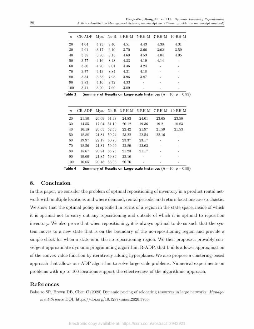
Benjaafar, Jiang, Li, and Li: Dynamic Inventory Repositioning
28 Article submitted to Management Science; manuscript no. (Please, provide the manuscript number!)
n CR-ADP Myo. No-R 3-RH-M 5-RH-M 7-RH-M 10-RH-M
20 4.04 4.73 9.40 4.51 4.43 4.38 4.31
30 2.91 3.17 6.10 3.70 3.66 3.62 3.59
40 3.35 3.96 8.15 4.60 4.53 4.04 4.05
50 3.77 4.16 8.48 4.33 4.19 4.14 -
60 3.80 4.20 9.01 4.36 4.24 - -
70 3.77 4.13 8.84 4.31 4.18 - -
80 3.34 3.83 7.93 3.96 3.87 - -
90 3.83 4.16 8.72 4.33 - - -
100 3.41 3.90 7.69 3.89 - - -
Table 3 Summary of Results on Large-scale Instances (n= 10, ρ= 0.95)
n CR-ADP Myo. No-R 3-RH-M 5-RH-M 7-RH-M 10-RH-M
20 21.50 26.09 61.98 24.83 24.01 23.65 23.50
30 14.55 17.04 51.10 20.12 19.36 19.21 18.83
40 16.18 20.63 52.46 22.42 21.97 21.59 21.53
50 18.88 21.81 59.24 23.22 22.54 22.16 -
60 19.97 22.17 60.70 23.37 23.17 - -
70 18.56 21.81 59.90 22.89 22.63 - -
80 15.67 20.24 55.75 21.23 21.17 - -
90 19.00 21.85 59.86 23.16 - - -
100 16.65 20.48 53.06 20.76 - - -
Table 4 Summary of Results on Large-scale Instances (n= 10, ρ= 0.99)
8. Conclusion
In this paper, we consider the problem of optimal repositioning of inventory in a product rental net-
work with multiple locations and where demand, rental periods, and return locations are stochastic.
We show that the optimal policy is specified in terms of a region in the state space, inside of which
it is optimal not to carry out any repositioning and outside of which it is optimal to reposition
inventory. We also prove that when repositioning, it is always optimal to do so such that the sys-
tem moves to a new state that is on the boundary of the no-repositioning region and provide a
simple check for when a state is in the no-repositioning region. We then propose a provably con-
vergent approximate dynamic programming algorithm, R-ADP, that builds a lower approximation
of the convex value function by iteratively adding hyperplanes. We also propose a clustering-based
approach that allows our ADP algorithm to solve large-scale problems. Numerical experiments on
problems with up to 100 locations support the effectiveness of the algorithmic approach.
References
Balseiro SR, Brown DB, Chen C (2020) Dynamic pricing of relocating resources in large networks. Manage-
ment Science DOI: https://doi.org/10.1287/mnsc.2020.3735.
Electronic copy available at: https://ssrn.com/abstract=2942921

Benjaafar, Jiang, Li, and Li: Dynamic Inventory Repositioning
Article submitted to Management Science; manuscript no. (Please, provide the manuscript number!) 29
Banerjee S, Freund D, Lykouris T (2017) Pricing and optimization in shared vehicle systems: An approxi-
mation framework, arXiv preprint arXiv:1608.06819.
Banerjee S, Kanoria Y, Qian P (2018) Dynamic assignment control of a closed queueing network under
complete resource pooling. arXiv e-prints arXiv–1803.
Belanger V, Ruiz A, Soriano P (2019) Recent optimization models and trends in location, relocation, and
dispatching of emergency medical vehicles. European Journal of Operational Research 272(1):1–23.
Benjaafar S, Wu S, Liu H, Gunnarsson EB (2021) Dimensioning on-demand vehicle sharing systems. Man-
agement Science DOI: https://doi.org/10.1287/mnsc.2021.3957.
Berman O (1981) Dynamic repositioning of indistinguishable service units on transportation networks. Trans-
portation Science 15(2):115–136.
Bertsekas DP, Tsitsiklis JN (1996) Neuro-Dynamic Programming (Belmont, MA: Athena Scientific).
Bimpikis K, Candogan O, Saban D (2019) Spatial pricing in ride-sharing networks. Operations Research
67(3):744–769.
Birge JR, Zhao G (2007) Successive linear approximation solution of infinite-horizon dynamic stochastic
programs. SIAM Journal on Optimization 18(4):1165–1186.
Boyd S, Boyd SP, Vandenberghe L (2004) Convex optimization (Cambridge university press).
Braverman A, Dai JG, Liu X, Ying L (2019) Empty-car routing in ridesharing systems. Operations Research
67(5):1437–1452.
Brown DB, Smith JE (2011) Dynamic portfolio optimization with transaction costs: Heuristics and dual
bounds. Management Science 57(10):1752–1770.
Bruglieri M, Colorni A, Lue A (2014) The vehicle relocation problem for the one-way electric vehicle sharing:
an application to the milan case. Procedia-Social and Behavioral Sciences 111:18–27.
Chen ZL, Powell WB (1999) Convergent cutting-plane and partial-sampling algorithm for multistage stochas-
tic linear programs with recourse. Journal of Optimization Theory and Applications 102(3):497–524.
Chung H, Freund D, Shmoys DB (2018) Bike Angels: An analysis of Citi Bike’s incentive program. Proceedings
of the 1st ACM SIGCAS Conference on Computing and Sustainable Societies (ACM).
Constantinides GM (1979) Multiperiod consumption and investment behavior with convex transactions costs.
Management Science 25(11):1127–1137.
De Farias DP, Van Roy B (2000) On the existence of fixed points for approximate value iteration and
temporal-difference learning. Journal of Optimization Theory and Applications 105(3):589–608.
Eberly JC, Van Mieghem JA (1997) Multi-factor dynamic investment under uncertainty. journal of economic
theory 75(2):345–387.
Freund D, Henderson SG, Shmoys DB (2017) Minimizing multimodular functions and allocating capacity in
bike-sharing systems. International Conference on Integer Programming and Combinatorial Optimiza-
tion, 186–198 (Springer).
Electronic copy available at: https://ssrn.com/abstract=2942921

Benjaafar, Jiang, Li, and Li: Dynamic Inventory Repositioning
30 Article submitted to Management Science; manuscript no. (Please, provide the manuscript number!)
Freund D, Henderson SG, Shmoys DB (2019) Bike sharing. Hu M, ed., Sharing Economy: Making Supply
Meet Demand (Springer).
Freund D, Norouzi-Fard A, Paul A, Henderson SG, Shmoys DB (2016) Data-driven rebalancing methods for
bike-share systems. Technical report.
George DK, Xia CH (2011) Fleet-sizing and service availability for a vehicle rental system via closed queueing
networks. European Journal of Operational Research 211:198–207.
Ghosh S, Varakantham P, Adulyasak Y, Jaillet P (2017) Dynamic repositioning to reduce lost demand in
bike sharing systems. Journal of Artificial Intelligence Research 58:387–430.
Girardeau P, Leclere V, Philpott AB (2014) On the convergence of decomposition methods for multistage
stochastic convex programs. Mathematics of Operations Research 40(1):130–145.
Godfrey GA, Powell WB (2001) An adaptive, distribution-free algorithm for the newsvendor problem with
censored demands, with applications to inventory and distribution. Management Science 47(8):1101–
1112.
He L, Hu Z, Zhang M (2020) Robust repositioning for vehicle sharing. Manufacturing & Service Operations
Management 22(2):241–256.
He L, Mak HY, Rong Y (2019) Operations management of vehicle sharing systems. Hu M, ed., Sharing
Economy: Making Supply Meet Demand (Springer).
He L, Mak HY, Rong Y, Shen ZJM (2017) Service region design for urban electric vehicle sharing systems.
Manufacturing & Service Operations Management 19(2):309–327.
Higle JL, Sen S (1991) Stochastic decomposition: An algorithm for two-stage linear programs with recourse.
Mathematics of Operations Research 16(3):650–669.
Jian N, Freund D, Wiberg HM, Henderson SG (2016) Simulation optimization for a large-scale bike-sharing
system. Proceedings of the 2016 Winter Simulation Conference, 602–613 (IEEE Press).
Jiang N, Kulesza A, Singh S, Lewis R (2015) The dependence of effective planning horizon on model accuracy.
Proceedings of the 2015 International Conference on Autonomous Agents and Multiagent Systems,
1181–1189 (Citeseer).
Kabra A, Belavina E, Girotra K (2020) Bike-share systems: Accessibility and availability. Management
Science 66(9):3803–3824.
Kaspi M, Raviv T, Tzur M (2017) Bike-sharing systems: User dissatisfaction in the presence of unusable
bicycles. IISE Transactions 49(2):144–158.
Kushner HJ, Yin GG (2003) Stochastic approximation and recursive algorithms and applications, volume 35
(Springer).
Lee CY, Meng Q (2015) Handbook of Ocean Container Transport Logistics (Springer).
Electronic copy available at: https://ssrn.com/abstract=2942921
Benjaafar, Jiang, Li, and Li: Dynamic Inventory Repositioning
Article submitted to Management Science; manuscript no. (Please, provide the manuscript number!) 31
Leland HE (1999) Optimal portfolio management with transactions costs and capital gains taxes, working
Paper RPF-290, IBER, UC Berkeley.
Li J, Leung CS, Wu Y, Liu K (2007) Allocation of empty containers between multi-ports. European Journal
of Operational Research 182(1):400–412.
Li Y, Zheng Y, Yang Q (2018) Dynamic bike reposition: A spatio-temporal reinforcement learning approach.
Proceedings of the 24th ACM SIGKDD Conference on Knowledge Discovery and Data Mining (ACM).
Li Z, Tao F (2010) On determining optimal fleet size and vehicle transfer policy for a car rental company.
Computers & operations research 37(2):341–350.
Lin LJ (1992) Self-improving reactive agents based on reinforcement learning, planning and teaching. Machine
Learning 8(3-4):293–321.
Linowsky K, Philpott AB (2005) On the convergence of sampling-based decomposition algorithms for mul-
tistage stochastic programs. Journal of Optimization Theory and Applications 125(2):349–366.
Liu J, Sun L, Chen W, Xiong H (2016) Rebalancing bike sharing systems: A multi-source data smart
optimization. Proceedings of the 22nd ACM SIGKDD Conference on Knowledge Discovery and Data
Mining, 1005–1014 (ACM).
Lu M, Chen Z, Shen S (2017) Optimizing the profitability and quality of service in carshare systems under
demand uncertainty. Manufacturing & Service Operations Management 20(2):162–180.
Ma H, Fang F, Parkes DC (2020) Spatio-temporal pricing for ridesharing platforms. ACM SIGecom
Exchanges 18(2):53–57.
Maxwell MS, Ni EC, Tong C, Henderson SG, Topaloglu H, Hunter SR (2014) A bound on the performance
of an optimal ambulance redeployment policy. Operations Research 62(5):1014–1027.
Maxwell MS, Restrepo M, Henderson SG, Topaloglu H (2010) Approximate dynamic programming for ambu-
lance redeployment. INFORMS Journal on Computing 22(2):266–281.
Mnih V, Kavukcuoglu K, Silver D, Rusu AA, Veness J, Bellemare MG, Graves A, Riedmiller M, Fidje-
land AK, Ostrovski G, et al. (2015) Human-level control through deep reinforcement learning. Nature
518(7540):529.
Munos R, Szepesvari C (2008) Finite-time bounds for fitted value iteration. Journal of Machine Learning
Research 9(May):815–857.
Muthuraman K, Kumar S (2006) Multidimensional portfolio optimization with proportional transaction
costs. Mathematical Finance: An International Journal of Mathematics, Statistics and Financial Eco-
nomics 16(2):301–335.
Nair R, Miller-Hooks E (2011) Fleet management for vehicle sharing operations. Transportation Science
45(4):524–540.
Nascimento JM, Powell WB (2009) An optimal approximate dynamic programming algorithm for the lagged
asset acquisition problem. Mathematics of Operations Research 34(1):210–237.
Electronic copy available at: https://ssrn.com/abstract=2942921

Benjaafar, Jiang, Li, and Li: Dynamic Inventory Repositioning
32 Article submitted to Management Science; manuscript no. (Please, provide the manuscript number!)
Nascimento JM, Powell WB (2010) Dynamic programming models and algorithms for the mutual fund cash
balance problem. Management Science 56(5):801–815.
Nyotta B, Bravo F, Feldman J (2019) Free rides in dockless, electric vehicle sharing systems Available at
SSRN: https://ssrn.com/abstract=3391937.
O’Mahony E, Shmoys DB (2015) Data analysis and optimization for (citi) bike sharing. AAAI, 687–694.
Pereira MVF, Pinto LMVG (1991) Multi-stage stochastic optimization applied to energy planning. Mathe-
matical Programming 52:359–375.
Philpott AB, Guan Z (2008) On the convergence of stochastic dual dynamic programming and related
methods. Operations Research Letters 36(4):450–455.
Porteus E (1982) Conditions for characterizing the structure of optimal strategies in infinite-horizon dynamic
programs. Journal of Optimization Theory and Applications 36(3):419–432.
Porteus EL (1975) On the optimality of structured policies in countable stage decision processes. Management
Science 22(2):148–157.
Powell WB (2007) Approximate Dynamic Programming: Solving the Curses of Dimensionality (John Wiley
& Sons), 2nd edition.
Powell WB, Ruszczynski A, Topaloglu H (2004) Learning algorithms for separable approximations of discrete
stochastic optimization problems. Mathematics of Operations Research 29(4):814–836.
Puterman ML (1994) Markov Decision Processes: Discrete Stochastic Dynamic Programming (New York,
NY, USA: John Wiley & Sons, Inc.), 1st edition.
Raviv T, Kolka O (2013) Optimal inventory management of a bike-sharing station. IIE Transactions
45(10):1077–1093.
Rockafellar RT (1970) Convex Analysis (Princeton, NJ, USA: Princeton University Press), 1st edition.
Schuijbroek J, Hampshire RC, Van Hoeve WJ (2017) Inventory rebalancing and vehicle routing in bike
sharing systems. European Journal of Operational Research 257(3):992–1004.
Shapiro A (2011) Analysis of stochastic dual dynamic programming method. European Journal of Operational
Research 209(1):63–72.
Shu J, Chou MC, Liu Q, Teo CP, Wang IL (2013) Models for effective deployment and redistribution of
bicycles within public bicycle-sharing systems. Operations Research 61(6):1346–1359.
Shui C, Szeto W (2018) Dynamic green bike repositioning problem–a hybrid rolling horizon artificial bee
colony algorithm approach. Transportation Research Part D: Transport and Environment 60:119–136.
Song DP (2005) Optimal threshold control of empty vehicle redistribution in two depot service systems.
IEEE Transactions on Automatic Control 50(1):87–90.
Sundararajan A (2016) The sharing economy: The end of employment and the rise of crowd-based capitalism
(Mit Press).
Electronic copy available at: https://ssrn.com/abstract=2942921
Benjaafar, Jiang, Li, and Li: Dynamic Inventory Repositioning
Article submitted to Management Science; manuscript no. (Please, provide the manuscript number!) 33
Van Mieghem JA (2003) Commissioned paper: Capacity management, investment, and hedging: Review and
recent developments. Manufacturing & Service Operations Management 5(4):269–302.
Warrington J, Beuchat PN, Lygeros J (2019) Generalized dual dynamic programming for infinite horizon
problems in continuous state and action spaces. IEEE Transactions on Automatic Control 64(12):5012–
5023.
Waserhole A, Jost V (2016) Pricing in vehicle sharing systems: Optimization in queuing networks with
product forms. EURO Journal on Transportation and Logistics 5(3):293–320.
Zhao L, Liu Z, Hu P (2020) Dynamic repositioning for vehicle sharing with setup costs. Operations Research
Letters 48(6):792–797.
Zipkin PH (2000) Foundations of Inventory Management (McGraw-Hill, New York).
Appendix A: Appendix
A.1. Empirical Justification of Assumption 1 and Estimation of P t
In this section, we describe our analysis of a publicly available Car2Go dataset15, which contains GPS
locations of Car2Go rental vehicles, at roughly 15-minute intervals, between June 2012 and December 2013
in Portland, Oregon. The goal is to understand whether Assumption 1 is realistic in practice. We use the
following procedure to obtain estimates of the return fraction pt specified in Assumption 1, calculated using
data from the entire year of 2013.
1. We assume hourly rental periods (i.e., repositioning occurs every hour) and that the city is divided into
n regions, 1,2, . . . , n.
2. For each vehicle, we extract all of its trips throughout the year under the assumption that trips end
when the vehicle remains at the same GPS coordinates between successive measurements (15 minutes). This
process yielded a total of 367,736 trips across 311 vehicles. Each trip is associated with a start time, return
time, rental origin, and return location.
3. For each hour t, we directly estimate the return fraction for each region i by computing the set of rentals
that are ongoing at hour t originating from region i (therefore, this includes any rental from i initiated at
or before t and returned strictly after t). The return fraction from region i is then the fraction of these trips
that are returned at hour t+ 1 (to any return location).
Table 5 shows the results of this estimation procedure for n= 9. These n= 9 regions are constructed using a
3x3 grid, defined by latitude regions (45.35,45.50], (45.50,45.55], and (45.55,45.82], and the longitude
regions (−122.86,−122.65], (−122.65,−122.60], and (−122.60,−121.65].
Assumption 1 states that the return fraction pt does not depend on the rental origin, but we compute these
quantities as if the dependency on rental origin is allowed. However, it can be seen that the variation of the
return fraction across regions is minor (i.e., the return fractions in each row are similar), thereby providing
empirical evidence that Assumption 1 is not unreasonable.
15 https://aaronparecki.com/car2go/
Electronic copy available at: https://ssrn.com/abstract=2942921

Benjaafar, Jiang, Li, and Li: Dynamic Inventory Repositioning
34 Article submitted to Management Science; manuscript no. (Please, provide the manuscript number!)
We also note that the return fraction matrix P t can be estimated using the same procedure that is outlined
above, assuming that GPS data is available. To obtain an estimate of pt,ij , we would simply alter Step 3
above to calculate the fraction of ongoing trips from region i that are returned specifically to region j at
hour t+ 1.
Time Period | Region 1 2 3 4 5 6 7 8 9
8am-9am 0.770 0.765 0.776 0.787 0.780 0.773 0.798 0.794 0.777
9am-10am 0.743 0.724 0.791 0.740 0.739 0.721 0.731 0.742 0.728
10am-11am 0.657 0.674 0.626 0.677 0.671 0.652 0.705 0.703 0.665
11am-12pm 0.644 0.681 0.642 0.671 0.681 0.660 0.668 0.697 0.671
12pm-1pm 0.693 0.659 0.664 0.661 0.684 0.676 0.655 0.705 0.655
1pm-2pm 0.642 0.664 0.714 0.642 0.682 0.636 0.650 0.696 0.686
2pm-3pm 0.697 0.650 0.611 0.655 0.688 0.668 0.684 0.693 0.630
3pm-4pm 0.656 0.647 0.651 0.680 0.671 0.644 0.660 0.668 0.650
4pm-5pm 0.667 0.654 0.616 0.664 0.676 0.651 0.633 0.632 0.630
5pm-6pm 0.664 0.696 0.644 0.700 0.727 0.690 0.687 0.706 0.698
Table 5 Estimates of Return Fraction pt (see Assumption 1) from 2013 Car2Go GPS Data
A.2. Properties of the Repositioning Cost
In this subsection, We describe some properties of the repositioning cost C(·) defined in (1).
Lemma 2. C(·) satisfies the following properties:
1. (Positive Homogeneity): C(tz) = tC(z) for all t≥ 0.
2. (Convexity): C(λz1 + (1−λ)z2)≤ λC(z1) + (1−λ)C(z2) for all z1,z2 ∈H and λ∈ [0,1].
3. (Sub-Additivity): C(z1 + z2)≤C(z1) +C(z2) for all z1,z2 ∈H.
4. (Continuity): C(z) is continuous in z ∈H.
Proof. It is clear that the linear program (1) is bounded feasible. Therefore, an optimal solution to (1)
exists and the strong duality holds. The dual linear program can be written as
C(z) = max λTz
subject to λj −λi ≤ cij ∀ i, j.(23)
From (23), we have
C(tz) = maxtλTz : λj −λi ≤ cij ,∀ i, j
= tmax
λTz : λj −λi ≤ cij ,∀ i, j
= tC(z).
Therefore, C(·) is positively homogeneous. As the pointwise supremum of a collection of convex and lower
semicontinuous functions (λTz for each λ), C(·) is also convex and lower semicontinuous. It is well known
that a convex function on a locally simplicial convex set is upper semicontinuous (Rockafellar (1970) Theorem
10.2). Therefore, as H is a polyhedron, C(·) must be continuous. From the positive homogeneity and the
convexity, we have
C(z1 + z2) = 2C
(1
2z1 +
1
2z2
)≤ 2
(1
2C(z1) +
1
2C(z2)
)=C(z1) +C(z2).
Therefore, C(·) is sub-additive.
Electronic copy available at: https://ssrn.com/abstract=2942921

Benjaafar, Jiang, Li, and Li: Dynamic Inventory Repositioning
Article submitted to Management Science; manuscript no. (Please, provide the manuscript number!) 35
Moreover, due to the triangle inequality, it is not optimal to simultaneously move inventory into and out of
the same location. This property can be stated as follows.
Lemma 3. There exists an optimal solution w to (1) such that
n∑
i=1
wij = z+j and
n∑
k=1
wjk = z−j for all j = 1, . . . , n.
Proof. It is easy to see that an equivalent condition is wi,jwj,k = 0 for all i, j, k. To show this is true,
suppose w is an optimal solution and there exists i, j, k such that wi,j ,wj,k > 0. If i= k, we can set at least
one of wi,j and wj,i to 0 without violating the constraints. If i 6= k, we can set at least one of wi,j and wj,k
to 0, and increase wi,k accordingly. In both cases, the resulting objective is at least as good. Repeating this
for all i, k and j can enforce this condition for all i, k and j.
Lemma 3 leads to the following bound for the repositioning cost C(z).
Lemma 4.cmin
2
n∑
i=1
|zi| ≤C(z)≤ cmax
2
n∑
i=1
|zi|. (24)
The proof follows from Lemma 3. There exists an optimal solution w to (1) such that
C(z) =∑
i,j
cijwij =1
2
∑
j
∑
i
cijwij +1
2
∑
j
∑
i
cjiwji
≤ cmax
2
∑
j
z+j +
cmax
2
∑
j
z−j =cmax
2
∑
j
|zj |.
It is easy to see that, in (24), the equality holds if cij = cmax for all i, j. Therefore, the bound is tight. The
lower bound follows the same logic.
A.3. Proof of Theorem 1
In this subsection, we provide a complete and self-contained proof for our main result, Theorem 1. We first
provide some basic properties for directional derivatives. Recall the definition of the directional derivative:
u′(x,γ;z,η) = limt↓0
u(x+ tz,γ+ tη)−u(x,γ)
t.
Lemma 5. If u(x,γ) is jointly convex in x and γ, then u′(x,γ;z,η) satisfies the following properties:
• (Positive Homogeneity) u′(x,γ; tz, tη) = tu′(x,γ;z,η)
• (Sub-Additivity) u′(x,γ;z1 + z2,η1 +η2)≤ u′(x,γ;z1,η1) +u′(x,γ;z2,η2).
Proof. These are well-known important properties for directional derivatives (see, for example, Rockafel-
lar (1970)).
Now, we establish the fact that if vt+1(·) is convex and additionally satisfies certain bounds on its directional
derivatives, then for any realization of dt,P t, the function Ut(yt,γt,dt,P t) can be reformulated as the convex
program (8).
Proposition 3. Suppose Assumptions 1 and 2 hold and
1. vt+1(xt+1,γt+1) is continuous and jointly convex in xt+1 and γt+1,
Electronic copy available at: https://ssrn.com/abstract=2942921

Benjaafar, Jiang, Li, and Li: Dynamic Inventory Repositioning
36 Article submitted to Management Science; manuscript no. (Please, provide the manuscript number!)
2. v′t+1(xt+1,γt+1;z−η,η)≤C(−z)+∑n
i=1(βi+ρcmax− cmin)ηi for any feasible direction (z−η,η) with
η≥ 0.
Then for all realizations (d,p), Ut(yt,γt,dt,P t) defined in (5) can be written as the following optimization
problem:Ut(yt,γt,dt,P t) = minw,xt+1,γt+1
∑n
i=1 βi(dt,i−wi) + ρvt+1(xt+1,γt+1)
s.t. xt+1 = yt−w+P Tt (γt +w);
γt+1 = (γt +w) (e−P te);
w≤ yt;w≤ dt.
(25)
Moreover, Ut(yt,γt,dt,P t) is continuous and jointly convex in yt and γt.
Proof. Let (w∗,x∗t+1,γ∗t+1) be the optimal solution to problem (25). Clearly, if w∗ = minyt,dt, the
reformulation is correct. Now suppose that there exist an index i such thatw∗ <minyt,dt. Let w=w∗+εei
for a small ε > 0. Then we have
xt+1 = yt− (w∗+ εei) +P Tt (γt +w∗+ εei) =x∗t+1 + ε(−ei +P T
t ei)
γt+1 = (γt +w∗+ εei) (e−P te) = γ∗t+1 + εei
(1−
n∑
j=1
Ptij
)= γ∗t+1 + εei (1− pt) ,
where the last inequality is based on Assumption 1. Let
z =P Tt ei−
n∑
j=1
Ptijei =P Tt ei− ptei, η= ei (1− pt) .
From the problem assumption, we have:
v′t+1
(xt+1,γt+1;−ei +P T
t ei,ei (1− pt))
= v′t+1(xt+1,γt+1; z− η, η)
≤ C(−z) +
n∑
j=1
(βi + ρcmax− cmin)ηj
≤ cmax
2‖z‖1 + (βi + ρcmax− cmin) (1− pt) (by Lemma 4)
≤ cmax
2
‖P Tei‖1 +
∥∥∥∥∥n∑
j=1
Pijei
∥∥∥∥∥1
+ (βi + ρcmax− cmin) (1− pt) (by the triangle inequality)
= cmaxpt + (βi + ρcmax− cmin) (1− pt) .
Let
f(w) =
n∑
i=1
βi(dt,i−wi) + ρvt+1(xt+1(w),γt+1(w)),
where xt+1(w),γt+1(w) are defined from the first two equalities. Then
∂f(w)
∂wi= −βi + ρv′t+1
(xt+1,γt+1;−ei +P T
t ei,ei (1− pt))
≤ −βi + ρcmaxpt + ρ(βi + ρcmax− cmin) (1− pt)
≤ −βi + ρcmaxpt + (βi + ρcmax− cmin) (1− pt) (since ρ≤ 1)
= ρcmax− cmin− pt(βi− cmin)≤ 0 (by Assumption 2).
Electronic copy available at: https://ssrn.com/abstract=2942921
Benjaafar, Jiang, Li, and Li: Dynamic Inventory Repositioning
Article submitted to Management Science; manuscript no. (Please, provide the manuscript number!) 37
Therefore, it is always optimal to increase wi for all yt,γt,dt,P t. This prove the first part of the proposition.
The continuity of u(·) follows from the Dominated Convergence Theorem, as Ut(yt,γt,dt,P t)≤∑
iβidi +
ρ‖v‖∞. For the convexity, since the constraint of the optimization problem is linear, thus the feasible region
is convex. Also vt+1(xt+1,γt+1) is jointly convex in xt+1 and γt+1, we have Ut(yt,γt,dt,P t) is jointly convex
in yt and γt (see, e.g., section 3.2.5 of Boyd et al. (2004)).
From Proposition 3, to show the convexity of ut(·), we require vt+1(·) to be convex and satisfy the bounds
on directional derivative as presented in item 2. If the convexity of ut(·) could imply the convexity and the
aforementioned bounds of directional derivation for vt(·), then the induction is complete. Unfortunately, the
convexity of ut(·) does not imply that
v′t+1(xt+1,γt+1;z−η,η)≤C(−z) +
n∑
i=1
(βi + ρcmax− cmin)ηi.
To overcome this difficulty, in Proposition 4, we assume a stronger condition on vt+1(·) that implies that
ut(·) satisfies two types of bounds on partial derivative as stated in the Theorem 1. Then in Proposition 5,
we show that if ut(·) is convex and satisfies these two types of bounds, vt(·) would be convex and satisfies
the stronger condition assumed in Proposition 4. This would complete the induction step.
Before we present Proposition 4, we first show how to decompose the directional derivative of Ut,d,p(·, ·),Ut(·, ·,d,p). Through this Lemma, we connect the directional derivatives of ut(·) and those of vt+1(·). We
define some notation for indices sets. For any vector y ∈Rn, we let J−(y) = i |yi < 0, J0(y) = i |yi = 0,J+(y) = i |yi > 0, J0+(y) = i |yi ≥ 0 and J0−(y) = i |yi ≤ 0.
Lemma 6. For any realization (d,P ), we have
U ′t,d,P (y,γ;z,η) =−
∑
i∈J−(y−d)∪(J0(y−d)∩J−(z))
βizi + ρv′t+1(x,ζ;w+,δ+), (26)
where
w+i =
zi + ιi +
∑j∈J−(y−d)∪(J0(y−d)∩J−(z)) zjpji for i∈ J+(y−d)∪ (J0(y−d)∩ J+(z)),
ιi +∑
j∈J−(y−d)∪(J0(y−d)∩J−(z)) zjpji for i∈ J−(y−d)∪ (J0(y−d)∩ J0−(z)),
with ιi ,∑n
j=1 ηjpji and
δ+i =
ηi(1−
∑n
j=1 pij) for i∈ J+(y−d)∪ (J0(y−d)∩ J+(z)),
(ηi + zi)(1−∑n
j=1 pij) for i∈ J−(y−d)∪ (J0(y−d)∩ J0−(z)),
and
x= τx(y,γ,d,P ); ζ = τγ(y,γ,d,P ).
Proof. Let
ϑi =
n∑
j=1
γjpji, ιi =
n∑
j=1
ηjpji
Note that
L(y,d) =∑
i∈J−(y−d)
βi(di− yi), (27)
Electronic copy available at: https://ssrn.com/abstract=2942921
Benjaafar, Jiang, Li, and Li: Dynamic Inventory Repositioning
38 Article submitted to Management Science; manuscript no. (Please, provide the manuscript number!)
and let the next state, under (d,P ), be defined by x(y,γ),ζ(y,γ), with components
xi(y,γ) =
(yi− di) +ϑi +
∑j∈J+(y−d) djpji +
∑j∈J0−(y−d) yjpji for i∈ J+(y−d),
ϑi +∑
j∈J+(y−d) djpji +∑
j∈J0−(y−d) yjpji for i∈ J0−(y−d),(28)
ζi(y,γ) =
(γi + di)(1−
∑n
j=1 pij) for i∈ J+(y−d),
(γi + yi)(1−∑n
j=1 pij) for i∈ J0−(y−d).(29)
Choose t small enough so that the following hold:
J−(y+ tz−d) = J−(y−d)∪ (J0(y−d)∩ J−(z)),
J0(y+ tz−d) = J0(y−d)∩ J0(z),
J+(y+ tz−d) = J+(y−d)∪ (J0(y−d)∩ J+(z)),
J0−(y+ tz−d) = J−(y−d)∪ (J0(y−d)∩ J0−(z)),
(30)
where the last equation follows directly from the first and second. For y+ tz, we have, directly by (27), that
L(y+ tz,d) =∑
i∈J−(y+tz−d)
βi(di− yi− tzi),
and directly from (28) and (29),
xi(y+ tz,γ+ tη)
=
yi + tzi− di +ϑi + tιi +∑
j∈J+(y+tz−d) djpji
+∑
j∈J0−(y+tz−d)(yj + tzj)pjifor i∈ J+(y+ tz−d),
ϑi + tιi +∑
j∈J+(y+tz−d) djpji
+∑
j∈J0−(y+tz−d)(yj + tzj)pjifor i∈ J0−(y+ tz−d),
and
ζi(y+ tz,γ+ tη) =
(γi + tηi + di)(1−
∑n
j=1 pi,j) for i∈ J+(y+ tz−d),
(γi + tηi + yi + tzi)(1−∑n
j=1 pi,j) for i∈ J0−(y+ tz−d).
It follows by (30) that
L(y+ tz,d)−L(y,d) =−t∑
i∈J−(y−d)∪(J0(y−d)∩J−(z))
βizi.
For the state update equations, we have
xi(y+ tz,γ+ tη)−xi(y,γ)
=
tzi + tιi +
∑j∈J−(y−d)∪(J0(y−d)∩J−(z)) tzjpji for i∈ J+(y−d)∪ (J0(y−d)∩ J+(z)),
tιi +∑
j∈J−(y−d)∪(J0(y−d)∩J−(z)) tzjpji for i∈ J−(y−d)∪ (J0(y−d)∩ J0−(z)),
and
ζi(y+ tz,γ+ tη)− ζi(y,γ)
=
tηi(1−
∑n
j=1 pij) for i∈ J+(y−d)∪ (J0(y−d)∩ J+(z)),
t(ηi + zi)(1−∑n
j=1 pij) for i∈ J−(y−d)∪ (J0(y−d)∩ J0−(z)).
Set
w+ =x(y+ tz,γ+ tη)−x(y,γ)
t, δ+ =
ζ(y+ tz,γ+ tη)− ζ(y,γ)
t.
Electronic copy available at: https://ssrn.com/abstract=2942921

Benjaafar, Jiang, Li, and Li: Dynamic Inventory Repositioning
Article submitted to Management Science; manuscript no. (Please, provide the manuscript number!) 39
Then
limt→0
vt+1(x(y+ tz,γ+ tη),ζ(y+ tz,γ+ tη))− vt+1(x(y,γ),ζ(y,γ))
t= v′t+1(x,ζ;w+,δ+).
It follows that
U ′t,d,p(y,γ;z,η) =−
∑
i∈J−(y−d)∪(J0(y−d)∩J−(z))
βizi + ρv′t+1(x,ζ;w+,δ+). (31)
This concludes the proof.
Now we are ready to present Proposition 4, which shows that given the convexity of vt+1(xt+1,γt+1) and
certain bounds on its directional derivatives, the function ut(yt,γt) satisfies two types of bounds on its
directional derivatives.
Proposition 4. Suppose Assumptions 1 and 2 hold and
1. vt+1(xt+1,γt+1) is continuous and jointly convex in xt+1 and γt+1,
2. v′t+1(xt+1,γt+1;z−η,η)≤C(−z)+∑n
i=1(βi+ρcmax− cmin)ηi for any feasible direction (z−η,η) with
η≥ 0,
3. v′t+1(xt+1,γt+1;z+η,−η)≤C(−z) +∑n
i=1 βiηi for any feasible direction (z+η,−η) with η≥ 0,
4. v′t+1(xt+1,γt+1;0,z)≤ (ρcmax/2)∑n
i=1 |zi| for any feasible direction (0,z) with eTz = 0,
then we have:
1. |u′t(yt,γt;∓ξ,±ξ)| ≤∑n
i=1 βiξi for all (yt,γt)∈∆ and any feasible direction (∓ξ,±ξ) with ξ≥ 0 ;
2. u′t(yt,γt;0,z)≤ (ρcmax/2)∑n
i=1 |zi| for all (yt,γt)∈∆ and any feasible direction (0,z) with eTz = 0.
Proof. We omit the subscript t to reduce notation. To show the first inequality, we start with showing
that u′(y,γ;−ξ,ξ)≤∑iβiξi. From Lemma 6, noting that −ξ≤ 0, we have
U ′d,p(y,γ;−ξ,ξ) =∑
i∈J−(y−d)∪J0(y−d)
βiξi + ρv′(x,γ;w− δ,δ),
where
wi =
−ξi
∑n
j=1 pij +∑
j∈J+(y−d) ξjpji for i∈ J+(y−d),∑j∈J+(y−d) ξjpji for i∈ J−(y−d)∪ J0(y−d),
and
δi =
ξi(1−
∑n
j=1 pij) = ξi(1− p) for i∈ J+(y−d),
0 for i∈ J−(y−d)∪ J0(y−d).
Note that eTw= 0 and so it is clear that (w− δ,δ) is a feasible direction at (x,ζ). It follows that
U ′d,p(y,γ;−ξ,ξ)
=∑
i∈J−(y−d)∪J0(y−d)
βiξi + ρv′(x,γ;w− δ,δ)
≤∑
i∈J−(y−d)∪(J0(y−d))
βi|ξi|+ ρC(−w) + ρ
n∑
i=1
(βi + ρcmax− cmin)|δi| (by assumption)
≤∑
i∈J−(y−d)∪(J0(y−d))
βi|ξi|+ρcmax
2
n∑
i=1
|wi|+ ρ
n∑
i=1
(βi + ρcmax− cmin)|δi| (by Lemma 4)
Electronic copy available at: https://ssrn.com/abstract=2942921
Benjaafar, Jiang, Li, and Li: Dynamic Inventory Repositioning
40 Article submitted to Management Science; manuscript no. (Please, provide the manuscript number!)
≤∑
i∈J−(y−d)∪(J0(y−d))
βi|ξi|+2ρcmax
2
n∑
i=1
∑
j∈J+(y−d)
|ξj |pji
+ ρ∑
i∈J+(y−d)
(βi + ρcmax− cmin)|ξi| (1− p) (by the triangle inequality)
=∑
i∈J−(y−d)∪(J0(y−d))
βi|ξi|+∑
j∈J+(y−d)
(pρcmax + ρ(βi + ρcmax− cmin)(1− p)) |ξj |
≤∑
i∈J−(y−d)∪(J0(y−d))
βi|ξi|+∑
j∈J+(y−d)
(pρcmax + (βi + ρcmax− cmin) (1− p)) |ξj |
≤∑
i∈J−(y−d)∪(J0(y−d))
βi|ξi|+∑
j∈J+(y−d)
(βi + (ρcmax− cmin)− p(βi− cmin)) |ξj |
≤∑
i∈J−(y−d)∪(J0(y−d))
βi|ξi|+∑
i∈J+(y−d)
βi|ξi| (by Assumption 2)
=
n∑
i=1
βi|ξi|
So, U ′d,p(y,γ;−ξ,ξ) ≤∑n
i=1 βi|ξi| =∑n
i=1 βiξi holds for each (y,γ) ∈∆ and (z − η,η) feasible. It follows
that u′(y,γ;−ξ,ξ) =∫U ′d,p(y,γ;−ξ,ξ)dµ≤∑
iβiξi. From Lemma 3, u(y,γ) is convex, thus
u′(y,γ;ξ,−ξ)≥−u′(y,γ;−ξ,ξ)≥−∑
i
βiξi.
Now we show that u′(y,γ;ξ,−ξ)≤∑n
i=1 βiξi for all (y,γ)∈∆ for all feasible direction (ξ,−ξ) with ξ≥ 0.
From the previous analysis, we have
U ′d,p(y,γ;ξ,−ξ) =−∑
i∈J−(y−d)
βiξi + ρv′(x,ζ;w+ δ,−δ)
where
wi =
ξi∑n
j=1 pij −∑
j∈J+(y−d)∪J0(y−d) ξjpji for i∈ J+(y−d)∪ J0(y−d),
−∑j∈J+(y−d)∪J0(y−d) ξjpji for i∈ J−(y−d),
δi =
ξi(1−
∑n
j=1 pij) = ξi(1− p) for i∈ J+(y−d)∪ J0(y−d),
0 for i∈ J−(y−d).
Clear (w+ δ,−δ) is a feasible direction at (x,ζ). It follows that
U ′d,p(y,γ;ξ,−ξ)
= −βi∑
i∈J−(y−d)
ξi + ρv′(x,γ;w+ δ,−δ)
≤ ρcmax
2
n∑
i=1
|wi|+ ρ
n∑
i=1
βi|δi| (from the third inequality of the assumption and ξ≥ 0)
≤ 1
2
n∑
i=1
βi|wi|+ ρ
n∑
i=1
βi|δi| (since ρcmax ≤ βi, ρ≤ 1)
≤ ρ
22
n∑
i=1
∑
j∈J+(y−d)∪J0(y−d)
βi|ξj |pji + ρ∑
i∈J+(y−d)∪J0(y−d)
βi|ξi|(
1−n∑
j=1
pij
)(by the triangle inequality)
≤ ρ∑
i∈J+(y−d)∪J0(y−d)
βi|ξi| ≤n∑
i=1
βi|ξi|.
Electronic copy available at: https://ssrn.com/abstract=2942921

Benjaafar, Jiang, Li, and Li: Dynamic Inventory Repositioning
Article submitted to Management Science; manuscript no. (Please, provide the manuscript number!) 41
So, U ′d,p(y,γ;ξ,−ξ)≤∑n
i=1 βi|ξi|=∑n
i=1 βiξi holds for each (y,γ) ∈∆ and (z+ η,−η) feasible. It follows
that u′(y,γ;ξ,−ξ) =∫U ′d,p(y,γ;ξ,−ξ)dµ≤∑
iβiξi. From Lemma 3, u(y,γ) is convex, thus
u′(y,γ;−ξ,ξ)≥−u′(y,γ;ξ,−ξ)≥−∑
i
βiξi.
Summing up all the above, we have shown the first inequality.
Now we show the second inequality. From Lemma 6, we have
U ′d,p(y,γ;0,z) = ρv′(x,γ; ι,z(1− p))
where ιi =∑n
j=1 zjpji ∀ i and p=∑n
j=1 pij (Assumption 1). Therefore,
n∑
i=1
ιi =
n∑
j=1
n∑
i=1
zjpji =
n∑
j=1
pzj = 0,
and eTz(1− p) = 0. It follows that
U ′d,p(y,γ;0,z) = ρv′(x,γ; ι,z(1− p))
≤ ρv′(x,γ; ι,0) + ρv′(x,γ;0,z(1− p)) (by subadditivity, Lemma 5)
≤ ρC(−ι) +ρ2cmax
2
n∑
i=1
|zi|(1− p) (by assumption)
≤ ρcmax
2
n∑
i=1
|ιi|+ρ2cmax
2
n∑
i=1
|zi|(1− p) (by Lemma 4)
≤ ρcmax
2
n∑
i=1
n∑
j=1
|zj |pji +ρ2cmax
2
n∑
i=1
|zi|(1− p) (by the triangle inequality)
≤ ρcmax
2
n∑
i=1
|zi|. (by the subadditivity)
So, U ′d,p(y,γ;0,z) ≤ (ρcmax/2)∑n
i=1 |zi| holds for all realizations (d,p). It follows that the integral also
satisfies the condition.
The upcoming result, Proposition 5, assists with the eventual induction over t by stating that if ut(yt,γt)
is convex and certain bounds on its directional derivatives are satisfied, then vt(xt,γt) not only is convex,
but also satisfies the bounds on the directional derivatives required by Proposition 4. Before continuing, we
introduce a technical lemma that carefully analyzes the optimal repositioning plan. The main difficulty in
showing Proposition 5 is that there exist some situations where xti > 0, but y∗ti = 0 where y∗t is the optimal
solution to vt(xt,γt). In this case, if we move along the direction z with zi < 0 starting from xt, we are
not able to move along this direction if we start from position y∗. Therefore, we would need to find another
direction such that it is feasible for position y∗, but the cost of repositioning can be controlled. This is the
main purpose of Lemma 7. This lemma plays a crucial role in the proof of Proposition 5.
Lemma 7. Suppose x,y ≥ 0 and eTx= eTy. Suppose x−η ≥ 0. Then there exists another vector ξ such
that: 1) y−ξ≥ 0, 2) eTξ= eTη, 3)∑n
j=1 |ξj−ηj | ≤ 2∑n
j=1 |ηj |, 4) C(y−ξ−x+η) =C(y−x)−C(ξ−η).
Moreover, if η≥ 0, we have ξ≥ 0 andn∑
j=1
ξi +1
2
n∑
j=1
|ξj − ηj | ≤n∑
j=1
ηj (32)
Electronic copy available at: https://ssrn.com/abstract=2942921

Benjaafar, Jiang, Li, and Li: Dynamic Inventory Repositioning
42 Article submitted to Management Science; manuscript no. (Please, provide the manuscript number!)
Proof. Let I = i |yi−ηi < 0. If I = ∅, we have y−η≥ 0 and we just find ξ= η. Thus in the followings,
we assume that I 6= ∅. We let J − = i |yi− xi ≤ 0 and J + = i |yi− xi > 0. Note that yi− xi < 0 ∀ i ∈ I,
so I ⊆J −.
Lemma 3 suggests that there exists w≥ 0 such that c ·w=C(y−x) and
yj −xj =
−∑
i∈J+ wji =−∑iwji for j ∈J −;∑
i∈J− wij =∑
iwij for j ∈J +.
The interpretation of the first case above is that locations j with more inventory than the target level yj
transfer inventory to locations that are below the target level. The second case is interpreted in an analogous
way. Let ξ be such that
ξj =
yj for j ∈ I;
ηj for j ∈J − \I;∑i∈I
ηi−yixi−yi
wij + ηj for j ∈J +.
We claim that ξ satisfies the desired properties. We first verify that yj− ξj ≥ 0. This is clearly true if j ∈J −
from the construction of ξ. Now let j ∈J +, then we have
yj − ξj = yj −∑
i∈I
ηi− yixi− yi
wij − ηj ≥ yj −∑
i∈I
wij − ηj ≥ yj −∑
i
wij − ηj = xj − ηj ≥ 0,
where the first inequality follows from xi ≥ ηi > yi for i ∈ I. Therefore, y− ξ ≥ 0 and part (1) is complete.
Also, using xj − yj =∑
j∈J+ wij , we have:
∑
j
ξj =∑
j∈I
yj +∑
j∈J−\I
ηj +∑
j∈J+
(∑
i∈I
ηi− yixi− yi
wij + ηj
)
=∑
j∈I
yj +∑
j∈(J−\I)∪J+
ηj +∑
i∈I
ηi− yixi− yi
(xi− yi) =∑
i
ηi,
verifying part (2). Note that:
ξj − ηj =
yj − ηj for j ∈ I;
0 for j ∈J −\I;∑i∈I
ηi−yixi−yi
wij for j ∈J +.
To show part (3), we haven∑
j=1
|ξj − ηj |= 2∑
j∈I
(ηj − yj)≤ 2
n∑
j=1
|ηj |.
To show that C(y− ξ−x+η)≤C(y−x)−C(ξ−η), let w be such that
wij =
(1− ηi−yi
xi−yi)wij for i∈ I;
wij for i /∈ I.
Then for all j ∈J +, we have
yj − ξj − (xj − ηj)−∑
i
wij +∑
i
wji
= (yj −xj)− ξj + ηj −∑
i∈I
wij −∑
i/∈I
wij
=∑
i
wij −∑
i∈I
ηi− yixi− yi
wij −∑
i
wij +∑
i∈I
ηi− yixi− yi
wij = 0,
Electronic copy available at: https://ssrn.com/abstract=2942921

Benjaafar, Jiang, Li, and Li: Dynamic Inventory Repositioning
Article submitted to Management Science; manuscript no. (Please, provide the manuscript number!) 43
where we used∑
iwji = 0. Similarly, for all j ∈ I, we have
xj − ηj − yj + ξj −∑
i
wji +∑
i
wij
= xj − ηj −∑
i
(1− ηj − yj
xj − yj
)wji
= xj −∑
i
wji− ηj −ηj − yjxj − yj
(yj −xj) = 0
and for all j ∈J −\I, we have
xj − ηj − yj + ξj −∑
i
wji +∑
i
wij = xj − yj −∑
i
wji = 0.
Therefore, we have shown that w is a feasible solution to the optimization problem for C(·) defined in (1)
at y− ξ−x+η. Thus, we have:
C(y− ξ−x+η) ≤∑
i,j
cijwij
=∑
i,j
cijwij −∑
i∈I
∑
j
cij
(ηi− yixi− yi
wij
)
= C(y−x)−∑
i∈I
∑
j∈J+
cij
(ηi− yixi− yi
wij
).
If we define w as
wij =
ηi−yixi−yi
wij for i∈ I, j ∈J +;
0 otherwise,
then we can check that w is a feasible solution to (1) at ξ−η. Therefore, we have
∑
i∈I
∑
j∈J+
cij
(ηi− yixi− yi
wij
)= c · w≥C(ξ−η).
Finally, we have
C(y− ξ−x+η)≤C(y−x)−∑
i∈I
∑
j∈J+
cij
(ηi− yixi− yi
wij
)≤C(y−x)−C(ξ−η).
Together with the subadditivity of C(·), we conclude that
C(y− ξ−x+η) =C(y−x)−C(ξ−η),
proving part (4). The last claim follows directly from the construction of ξ and parts (2) and (3).
Now we are ready to prove Proposition 5.
Proposition 5. Suppose ut(·) is convex and continuous in ∆ and
1. u′t(yt,γt;±η,∓η)≤∑n
i=1 βiηi for all (yt,γt)∈∆ and for any feasible direction (±η,∓η) with η≥ 0;
2. u′t(yt,γt;0,z)≤ (ρcmax/2)∑n
i=1 |zi| for all (yt,γt)∈∆ and for any feasible direction (0,z) with eTz =
0.
Electronic copy available at: https://ssrn.com/abstract=2942921

Benjaafar, Jiang, Li, and Li: Dynamic Inventory Repositioning
44 Article submitted to Management Science; manuscript no. (Please, provide the manuscript number!)
Then, the value function vt(·) is convex and continuous in ∆ with Ωv(γ) = ∆n−1(I) for γ ∈ S. For each
(xt,γt)∈∆ and η≥ 0, the directional derivatives satisfy
v′t(xt,γt;z−η,η)≤C(−z) +
n∑
i=1
(βi + ρcmax− cmin)ηi (33)
for any feasible direction (z−η,η) and
v′t(xt,γt;z+η,−η)≤C(−z) +
n∑
i=1
βiηi (34)
for any feasible direction (z+η,−η). In addition,
v′t(xt,γt;0,z)≤ ρcmax
2
n∑
i=1
|zi| (35)
for any feasible direction (0,z) with eTz = 0.
Proof. We omit the subscript t throughout the proof to reduce notation. To show that v(·) is convex,
suppose y1 and y2 are optimal solutions of (16) for (x1,γ1) and (x2,γ2), respectively. Then, λy1 +(1−λ)y2 ∈∆n−1(λeTx1 + (1−λ)eTx2) and thus
v(λx1 + (1−λ)x2, λγ1 + (1−λ)γ2)≤ u(λx1 + (1−λ)x2, λγ1 + (1−λ)γ2)
+C(λ(y1−x1) + (1−λ)(y2−x2))
≤ λv(x1,γ1) + (1−λ)v(x2,γ2),
by convexity of u(·) and Lemma 2. Continuity follows from Berge’s Maximum Theorem, as the set-valued
map x 7→∆n−1(I) is continuous. To show the result in (33), suppose (z−η,η) is a feasible direction. Let y∗
be an optimal solution to equation (16) at (x,γ). Therefore,
v(x,γ) = miny∈∆n−1(eTx)
C(y−x) +u(y,γ) =C(y∗−x) +u(y∗,γ).
Let t > 0 be small enough such that x+ t(z − η) ≥ 0. According to Lemma 7, there exists a vector ξ ≥ 0
such that for small enough t: 1) y∗− tξ≥ 0, 2) eTξ= eTη, 3) 4) C(y∗− tξ−x− tz+ tη) =C(y∗−x− tz)−tC(ξ−η). Therefore, y∗− tξ is a feasible solution to equation (16) at (x+ tz− tη,γ+ tη) and thus we have
v(x+ tz− tη,γ+ tη)− v(x,γ)
t
≤ u(y∗− tξ,γ+ tη)−u(y∗− tξ,γ+ tξ) +u(y∗− tξ,γ+ tξ)−u(y∗,γ)
t
+C(y∗− tξ−x− tz+ tη)−C(y∗−x− tz) +C(y∗−x− tz)−C(y∗−x)
t
≤ u(y∗− tξ,γ+ tη)−u(y∗− tξ,γ+ tξ) +u(y∗− tξ,γ+ tξ)−u(y∗,γ)
t−C(ξ−η) +C(−z)
Adding and subtracting u(y∗,γ) in the numerator of the first term and then taking limits on both sides, we
get
v′(x,γ;z−η,η) ≤ u′(y∗,γ;−ξ,η)−u′(y∗,γ;−ξ,ξ) +u′(y∗,γ;−ξ,ξ)−C(ξ−η) +C(−z)
≤ u′(y∗,γ; 0,η− ξ) +u′(y∗,γ;−ξ,ξ)−C(ξ−η) +C(−z)
Electronic copy available at: https://ssrn.com/abstract=2942921
Benjaafar, Jiang, Li, and Li: Dynamic Inventory Repositioning
Article submitted to Management Science; manuscript no. (Please, provide the manuscript number!) 45
≤ ρ
2cmax
n∑
i=1
|ξi− ηi|+n∑
i=1
βiξi−cmin
2
n∑
i=1
|ξi− ηi|+C(−z)
≤n∑
i=1
βiηi +ρcmax− cmin
2
n∑
i=1
|ξi− ηi|+C(−z)
≤n∑
i=1
(βi + ρcmax− cmin)ηi +C(−z),
where the second inequality follows by Lemma 5 and the third inequality follows by Lemma 4.
Now we show equation (34). Suppose (z+η,−η) is a feasible direction. Again, let y∗ be an optimal solution
to equation (16) at (x,γ). Then y∗+ tη is clearly a feasible solution to equation (16) at (x+ tz+ tη,γ− tη)
and thus we have
v′(x,γ;z+η,−η) = limt→0
v(x+ tz+ tη,γ− tη)− v(x,γ)
t
≤ limt→0
u(y∗+ tη,γ− tη) +C(y∗−x− tz)−u(y∗,γ)−C(y∗−x)
t
≤ u′(y∗,γ;η,−η) +C(−z)
≤n∑
i=1
βiηi +C(−z),
where the second inequality follows from the subadditivity and the postive homogeneity of C(·) and the last
inequality follows from the assumption.
To show the result in (33), suppose (0,z) is a feasible direction at (x,γ). Let y∗ be an optimal solution
to equation (16) at (x,γ). Then y∗ is a feasible solution for (x,γ+ tz) and thus,
v′(x,γ;0,z) = limt→0
v(x,γ+ tz)− v(x,γ)
t
≤ limt→0
u(y∗,γ+ tz) +C(x−y∗)−u(y∗,γ)−C(x−y∗)t
= limt→0
u(y∗,γ+ tz)−u(y∗,γ)
t= u′(y∗,γ;0,z)≤ ρcmax
2
n∑
i=1
|zi|,
which completes the proof.
The last piece of Theorem 1 is the Lipschitz continuity of ut(·). In the next proposition, we show that item
(1) and (1) imply item (1).
Lemma 8. Consider a bounded function f : ∆→R that is convex, continuous, and satisfies
1. |f ′(y,γ;∓η,±η)| ≤∑n
i=1 βiηi for all (x,γ)∈∆ and any feasible direction (∓η,±η) with η≥ 0;
2. f ′(y,γ;0,v)≤ (ρcmax/2)∑n
i=1 |vi| for all (x,γ)∈∆ and any feasible direction (0,v) with eTv= 0.
Then, the function f(·) is Lipschitz continuous on ∆ with Lipschitz constant (3/2)√
2nβi.
Proof. Let (y,γ) ∈∆. Let ξ+ = max(ξ,0) and ξ− = min(ξ,0), then (ξ,η) = (ξ+,−ξ+) + (ξ−,−ξ−) +
(0,ξ+ + ξ−+η) and it follows from Theorem 2 and Assumption 2 that
|f ′(y,γ;ξ,η)| ≤ |f ′(y,γ;ξ+,−ξ+)|+ |f ′(y,γ;ξ−,−ξ−)|+ |f ′(y,γ; 0,ξ+ + ξ−+η)|
≤n∑
i=1
βi|ξ+i |+
n∑
i=1
βi|ξ−i |+ (ρcmax/2)‖ξ+ + ξ−+η‖1
≤ βmax ‖ξ‖1 + (ρcmax/2)‖ξ+ + ξ−+η‖1≤ βmax ‖ξ‖1 + (βmax/2)
(‖ξ+‖1 + ‖ξ−‖1 + ‖η‖1
)
≤ (3/2)βmax ‖(ξ,η)‖1 ≤ (3/2)√
2nβmax ‖(ξ,η)‖2.
Electronic copy available at: https://ssrn.com/abstract=2942921

Benjaafar, Jiang, Li, and Li: Dynamic Inventory Repositioning
46 Article submitted to Management Science; manuscript no. (Please, provide the manuscript number!)
With all the pieces ready, the proofs for Theorem 1 for (ut(·)) and (vt(·)) thus follow from Proposition 3,
Proposition 4, Proposition 5, and the induction.
A.4. Other Proofs
Proof of Theorem 3: Fix γ ∈ S. Let y∗(x,γ) = y ∈∆n−1(I) : u(x,γ) =C(y−x) +u(y,γ) be the set of
optimal solutions corresponding to the system state x∈ S. It is easy to verify that
Ωu(γ) =∪x∈∆n−1(I)y∗(x,γ). (36)
As C(·) and u(·) are continuous and ∆n−1(I) is compact, by Berge’s Maximum Theorem, y∗(·) is a nonempty-
valued and compact-valued upper hemicontinuous16 correspondence. As C(·) and u(·) are also convex, y∗(·)is also convex-valued. So, it is clear from (36) that Ωu(γ) is nonempty. To show Ωu(γ) is compact, suppose
y1,y2, . . . is a sequence in Ωu(γ) such that yn ∈ y∗(xn,γ) for n ∈ N and yn → y. We need to show that
y ∈Ωu(γ). By passing through a subsequence, we may assume that ynk ∈ y∗(xnk ,γ), xnk →x and ynk → y.
As y∗(·) is compact-valued, by the Closed Graph Theorem, y∗(·) has a closed graph. This implies that
y ∈ y∗(x,γ)⊂Ωu(γ), and therefore Ωu(γ) is compact.
To show that Ωu(γ) is connected, suppose the reverse is true. Then, there exist open sets V1, V2 in ∆n−1(I)
such that V1 ∩ V2 = ∅, V1 ∪ V2 ⊃ Ωu(γ), and V1 ∩Ωu(γ) and V2 ∩Ωu(γ) are nonempty. As y∗(·) is convex-
valued, this implies that, for any x∈∆n−1(I), y∗(x,γ) is either in V1 or in V2, but not both. Let (U1,γ) =
y∗−1(V1) and (U2,γ) = y∗−1(V2). Then U1,U2 are open, U1 ∩U2 = ∅, U1 ∪U2 ⊃∆n−1(I), and U1 ∩∆n−1(I)
and U2∩∆n−1(I) are nonempty. This implies that the (n−1)-dimensional simplex ∆n−1(I) is not connected.
We have reached a contradiction. Therefore, Ωu(γ) is also connected.
Next, to show that π∗ is optimal, note that π∗(x,γ) = x for x ∈ Ωu(γ) is clear from (17). If x /∈ Ωu(γ),
then, by (36), π∗(x,γ)∈Ωu(γ). Now, suppose there exists π∗(x,γ) = y ∈Ωu(γ), then y+ t(x−y)∈Ωu(γ)
for small enough t > 0. Set z = y + t(x− y). Then u(z,γ) +C(z − x) ≤ u(y,γ) +C(y − z) +C(z − x) =
u(y,γ) + tC(y−x) + (1− t)C(y−x) = u(y,γ) +C(y−x). So, z is as good a solution as y. Therefore, there
exists an optimal solution π∗(x,γ)∈B(Ωu(γ)) if x /∈Ωu(γ).
Proof of Proposition 1: Suppose x∈Ωu(γ). Take any feasible direction (z,0) at (x,γ). Then, by (17),
u(x+ tz,γ)−u(x,γ)
t≥−C(z)
for t > 0. Taking the limit as t ↓ 0, we have u′(x,γ;z,0)≥−C(z). Conversely, suppose u′(x,γ;z,0)≥−C(z)
for any feasible direction z at x in H. Let φ(t) = u(x + tz,γ). Then, φ(·) is convex, φ(0) = u(x), and
φ′(0+) = u′(x,γ;z,0) ≥ −C(z). By the subgradient inequality, tφ′(0+) + φ(0) ≤ φ(t). This implies that
−tC(z) +u(x,γ)≤ u(x+ tz,γ) is true for any feasible direction (z,0). Therefore, we have x∈Ωu(γ).
16 Upper hemicontinuity can be defined as follows. Suppose X and Y are topological spaces. A correspondencef :X→P(Y ) (power set of Y ) is upper hemicontinuous if for any open set V in Y , f−1(V ) = x ∈X|f(x)⊂ V isopen in X.
Electronic copy available at: https://ssrn.com/abstract=2942921

Benjaafar, Jiang, Li, and Li: Dynamic Inventory Repositioning
Article submitted to Management Science; manuscript no. (Please, provide the manuscript number!) 47
Proof of Proposition 2: For the “if” part, suppose x /∈Ωu(γ). Then, there exists y ∈∆n−1(I) such that
u(x,γ)>C(y−x) + u(y,γ). Take any g ∈ ∂xu(x,γ). By the subgradient inequality, u(x,γ) + gT (y−x)≤u(y,γ). It follows that
C(y−x)<−gT (y−x).
Suppose w= (wij) is an optimal solution to problem (1). Then C(y−x) =∑
i
∑j cijwij , and by Lemma 3,
−gT (y−x) =∑
i gi(yi−xi)−−∑
j gj(yj −xj)+ =∑
i
∑j(gi− gj)wij . So, we have
∑
i
∑
j
cijzij <∑
i
∑
j
(gi− gj)wij .
Hence, there exists i and j such that gi− gj > cij . This implies g /∈ G.
For the “only if” part, suppose x> 0 and x∈Ωu(γ). Assume ∂xu(x,γ)∩G = ∅. We will show that this leads
to a contradiction. Let P be the orthogonal projection from Rn to the subspace H= x ∈ Rn :∑
ixi = 0.
Then
P (x) =x−∑
ixin
e,
where e= (1, . . . ,1) in Rn. Noting that G+αe⊂G for any α∈R, it is easy to verify that
∂xu(x,γ)∩G = ∅ if and only if ∂xu(x,γ)∩P (G) = ∅,
since ∂xu(x,γ) ⊆H. As ∂xu(x,γ) is closed and P (G) is compact, by Hahn-Banach Theorem, there exists
z ∈H, a∈R and b∈R such that
〈g,z〉<a< b< 〈λ,z〉
for every g ∈ P (∂xu(x,γ)) and for every λ ∈ P (G), or equivalently, as 〈g,z〉 = 〈P (g),z〉 and 〈λ,z〉 =
〈P (λ),z〉, for every g ∈ ∂xu(x,γ) and for every λ ∈ G. As z is a feasible direction in H at x ∈ Ωu(γ), by
Proposition 1, we have u′(x,γ;z,0)≥−C(z). It follows that
sup〈g,z〉 : g ∈ ∂xu(x,γ)= u′(x,γ;z,0)≥−C(z).
So, we have
−C(z)≤ a< b< 〈λ,z〉
for every λ ∈ G. However, by the dual formulation (23), there exists λ ∈ (y1, y2 . . . , yn) |yj − yi ≤ cij ∀ i, jsuch that 〈λ,z〉=C(z), or equivalently, 〈−λ,z〉=−C(z). Recognizing that −λ ∈ G leads to the contradic-
tion. Therefore, it follows that ∂xu(x,γ)∩G 6= ∅.
Proof of Corollary 2: If u(·,γ) is differentiable at x, then
∂xu(x,γ) =
(∂u(x,γ)
∂x1
,∂u(x,γ)
∂x2
, . . . ,∂u(x,γ)
∂xn
).
In this case, it is easy to see that (??) is simplified to (??). To show that x ∈ Ωu(γ) implies (??) for x ∈B(∆n−1(I)). Note that the equality supgTz : g ∈ ∂xu(x,γ)= u′(x,γ;z,0) now holds for x ∈ B(∆n−1(I)).
The rest of the proof is the same as Proposition 2.
Electronic copy available at: https://ssrn.com/abstract=2942921
Benjaafar, Jiang, Li, and Li: Dynamic Inventory Repositioning
48 Article submitted to Management Science; manuscript no. (Please, provide the manuscript number!)
Proof of Theorem 2: To show that value function retains its structure in the infinite horizon setting, we
invoke the general approach outlined in Porteus (1975) and Porteus (1982) which “iterates” the structural
properties of the one-stage problem. Let V∗ be the space of convex, continuous and bounded functions over ∆.
Note that a one-step structure preservation property holds by Lemma 3, Lemma 4, and Lemma 5: combined,
they say that if the next period value function is in V∗, then the optimal value of the current period is also
in V∗. Furthermore, the set V∗ with the sup-norm ‖ · ‖∞ is a complete metric space. These two observations
allow us to apply Corollary 1 of Porteus (1975) and conclude that v ∈ V∗ (the remaining assumptions needed
to apply the result can be easily checked). The rest of the proof follows from Lemma 3, Lemma 4, Lemma
5, Theorem 3, Proposition 1, Proposition 2, and Corollary 2.
Proof of Lemma 1: If x∈Dk, ak ∈ ∂xuJ(x,γ). Since aki−akj ≤ cij for all i, j, according to Proposition 2,
we have x∈ΩuJ (ζ). For the second part, we first write down the primal formulation for problem (??):
vJ(x,ζ) = min c ·w+ ξ
subject to
n∑
i=1
wi,j −n∑
k=1
wj,k = zj −xj ∀ j = 1,2, . . . , n
w≥ 0
eTz = eTx
ξ ≥ (z−yk)Tak + (ζ−γk)Tbk + ιk ∀k= 1,2, . . . , J
z ≥ 0.
Since x ∈ ΩuJ (ζ), one optimal solution to the primal formulation is w = 0,z = x, ξ = (x− yk)Tak + (γ −γk)
Tbk + ιk. The dual solution λ= ak, µk = 1, µl = 0,∀ l 6= k is clearly feasible. It also satisfies the comple-
mentary slackness condition. Therefore, the solution is optimal.
Proof of Theorem 4: Let us first introduce some notation. For any bounded function f : ∆→R, we define
the mapping L such that Lf : ∆→R is another bounded function such that
(Lf)(y,γ) = l(y) + ρ
∫min
y′∈∆n−1(eTx′)C(y′−x′) + f(y′,γ′)dµ ∀ (y,γ)∈∆, (37)
where x′ = τx(y,γ,d,P ) and γ′ = τγ(y,γ,d,P ). Note that L is closely related to the standard Bellman
operator associated with the MDP defined in (9); see, for example, Bertsekas and Tsitsiklis (1996). The
difference from the standard definition is that L comes from the Bellman recursion for u(y,γ) instead of
v(x,γ). With this in mind, we henceforth simply refer to L as the “Bellman operator” and note a few
standard properties.
Lemma 9. The Bellman operator L has the following properties:
1. (Monotonicity) Given bounded f1, f2 : ∆→R with f1 ≤ f2, then Lf1 ≤Lf2.
2. (Contraction) For any bounded f1, f2 : ∆→R, it holds that ‖Lf1−Lf2‖∞ ≤ ρ‖f1− f2‖∞.
3. (Fixed Point) The optimal value function u is the unique fixed point of L, i.e., Lu= u.
4. (Constant Shift) Let 1 be the constant one function, i.e., 1(·) = 1, and let α be a scalar. For any bounded
f : ∆→R, it holds that L(f +α1) =Lf + ρα1.
Electronic copy available at: https://ssrn.com/abstract=2942921

Benjaafar, Jiang, Li, and Li: Dynamic Inventory Repositioning
Article submitted to Management Science; manuscript no. (Please, provide the manuscript number!) 49
Proof. These basic properties for our Bellman operator L are well-known for the standard Bellman
operator and can be proved in an analogous manner; see, for example, Puterman (1994) or Bertsekas and
Tsitsiklis (1996).
We now move on to the main proof. We want to show that for each ε > 0, there exists an almost surely
finite iteration index J(ε) such that for all J ≥ J(ε), it holds that ‖uJ −u‖∞ ≤ ε. Let Br(y,γ) be a (2n− 1)-
dimensional ball centered at (y,γ) ∈ ∆ with radius r. Consider some ε′ > 0 (to be specified later) and
let C(ε′) be an ε′-covering of ∆, meaning that C(ε′) is a finite collection of points in ∆ (representing the
centers of a finite collection of balls with radius ε′) and ∆⊆⋃(y,γ)∈C(ε′)Bε′(y,γ). Let (y1, γ1), (y2, γ2), . . .
denote the sequence of sample points visited by the algorithm (one per iteration). Thus, by Assumption 3,
we have∑
JP(yJ , γJ)∈Bε′(y,γ)=∞, and an application of the Borel-Cantelli lemma tells us that each
ball Bε′(y,γ) associated with the covering is visited infinitely often with probability one. To reduce notation,
we will often suppress (y,γ) and use Bε′ to denote a generic ball in the covering. Our proof follows three
main ideas:
1. For any infinite trajectory of sampled states, we can split it into an infinite number of “phases” such
that in each phase, every ball associated with the ε′-covering is visited at least once.
2. We can then construct an auxiliary “batch” algorithm whose iteration counter aligns with the sequence
of phases from the previous step. This new algorithm is defined as another instance of Algorithm 1, where on
any given iteration, we group all states visited in the corresponding phase of the main algorithm into a single
batch and perform all updates at once. For clarity, we will refer to the main algorithm as the “asynchronous”
version of the batch algorithm.
3. The auxiliary batch algorithm can be viewed as an approximate version of value iteration. Using the
properties of L, we can show that it converges to an approximation of u (with error depending on ε′). Finally,
we conclude by arguing that the main algorithm does not deviate too far from the auxiliary version.
Let J0 = 0 and for K = 1,2, . . ., define the random variable
JK+1 = minJ > JK : ∀ (y,γ)∈ C(ε′), ∃J ′ s.t. JK <J′ ≤ J, (yJ′ , γJ′)∈Bε′(y,γ)
to be the first time after JK such that every ball in the ε′-covering is visited at least once. Notably, J1 is the
first time that the entire covering is visited at least once. We denote the set of iterations
JK = JK−1 + 1, JK−1 + 2, . . . , JK
to be the “Kth phase” of the algorithm and let SK = (yJ , γJ)J∈JK be the set of states visited throughout
the course of phase K.
We now describe “path-dependent” instances of Algorithm 1 to assist with the remaining analysis. To
be precise with the definitions, let us consider a sample path ω. The auxiliary batch algorithm associated
with ω is a new instance of Algorithm 1 that uses iteration counter K and generates hyperplanes at the set
of states SK = SK(ω) for all K ≥ 1. The initial approximation is u0 = u0 and the estimate after K batch
updates is denoted uK(y,γ)(ω) = maxi=1,...,NK gi(y,γ)(ω). We are now interested in studying the stochastic
process uK(y,γ).
Electronic copy available at: https://ssrn.com/abstract=2942921
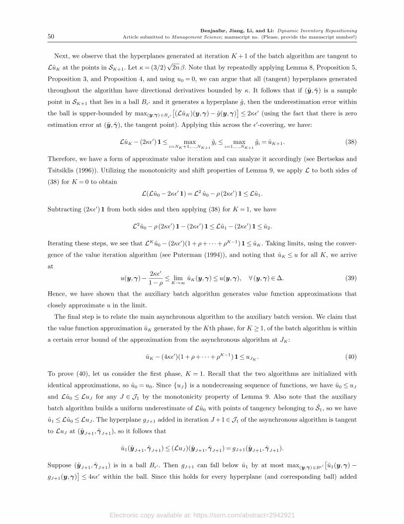
Benjaafar, Jiang, Li, and Li: Dynamic Inventory Repositioning
50 Article submitted to Management Science; manuscript no. (Please, provide the manuscript number!)
Next, we observe that the hyperplanes generated at iteration K+ 1 of the batch algorithm are tangent to
LuK at the points in SK+1. Let κ= (3/2)√
2nβ. Note that by repeatedly applying Lemma 8, Proposition 5,
Proposition 3, and Proposition 4, and using u0 = 0, we can argue that all (tangent) hyperplanes generated
throughout the algorithm have directional derivatives bounded by κ. It follows that if (y, γ) is a sample
point in SK+1 that lies in a ball Bε′ and it generates a hyperplane g, then the underestimation error within
the ball is upper-bounded by max(y,γ)∈Bε′
[(LuK)(y,γ)− g(y,γ)
]≤ 2κε′ (using the fact that there is zero
estimation error at (y, γ), the tangent point). Applying this across the ε′-covering, we have:
LuK − (2κε′)1≤ maxi=NK+1,...,NK+1
gi ≤ maxi=1,...,NK+1
gi = uK+1. (38)
Therefore, we have a form of approximate value iteration and can analyze it accordingly (see Bertsekas and
Tsitsiklis (1996)). Utilizing the monotonicity and shift properties of Lemma 9, we apply L to both sides of
(38) for K = 0 to obtain
L(Lu0− 2κε′ 1) =L2 u0− ρ (2κε′)1≤Lu1.
Subtracting (2κε′)1 from both sides and then applying (38) for K = 1, we have
L2u0− ρ (2κε′)1− (2κε′)1≤Lu1− (2κε′)1≤ u2.
Iterating these steps, we see that LK u0− (2κε′)(1 + ρ+ · · ·+ ρK−1)1≤ uK . Taking limits, using the conver-
gence of the value iteration algorithm (see Puterman (1994)), and noting that uK ≤ u for all K, we arrive
at
u(y,γ)− 2κε′
1− ρ ≤ limK→∞
uK(y,γ)≤ u(y,γ), ∀ (y,γ)∈∆. (39)
Hence, we have shown that the auxiliary batch algorithm generates value function approximations that
closely approximate u in the limit.
The final step is to relate the main asynchronous algorithm to the auxiliary batch version. We claim that
the value function approximation uK generated by the Kth phase, for K ≥ 1, of the batch algorithm is within
a certain error bound of the approximation from the asynchronous algorithm at JK :
uK − (4κε′)(1 + ρ+ · · ·+ ρK−1)1≤ uJK . (40)
To prove (40), let us consider the first phase, K = 1. Recall that the two algorithms are initialized with
identical approximations, so u0 = u0. Since uJ is a nondecreasing sequence of functions, we have u0 ≤ uJand Lu0 ≤ LuJ for any J ∈ J1 by the monotonicity property of Lemma 9. Also note that the auxiliary
batch algorithm builds a uniform underestimate of Lu0 with points of tangency belonging to S1, so we have
u1 ≤Lu0 ≤LuJ . The hyperplane gJ+1 added in iteration J+1∈J1 of the asynchronous algorithm is tangent
to LuJ at (yJ+1, γJ+1), so it follows that
u1(yJ+1, γJ+1)≤ (LuJ)(yJ+1, γJ+1) = gJ+1(yJ+1, γJ+1).
Suppose (yJ+1, γJ+1) is in a ball Bε′ . Then gJ+1 can fall below u1 by at most max(y,γ)∈Bε′[u1(y,γ) −
gJ+1(y,γ)]≤ 4κε′ within the ball. Since this holds for every hyperplane (and corresponding ball) added
Electronic copy available at: https://ssrn.com/abstract=2942921

Benjaafar, Jiang, Li, and Li: Dynamic Inventory Repositioning
Article submitted to Management Science; manuscript no. (Please, provide the manuscript number!) 51
throughout the phase K = 1 and noting that every point in ∆ can be associated with some well-approximating
hyperplane (due to the property that each phase contains at least one visit to every ball), we have
u1− (4κε′)1≤ maxJ=1,...,J1
gJ = uJ1 , (41)
which proves (40) for K = 1. Applying L to both sides of (41), utilizing Lemma 9, noting that u2 underesti-
mates Lu1, and applying the nondecreasing property of the sequence uJ, we have
u2− ρ (4κε′)1≤Lu1− ρ (4κε′)1≤LuJ1 ≤LuJ , ∀J ∈J2.
By the same reasoning as above, for J + 1∈J2, it must hold that
u2(yJ+1, γJ+1)− ρ (4κε′)≤ (LuJ)(yJ+1, γJ+1) = gJ+1(yJ+1, γJ+1),
and we obtain u2 − ρ (4κε′)1− (4κε′)1≤ uJ2 , proving (40) for K = 2. We can iterate these steps to argue
(40) for any K. Taking limits (all subsequent limits exist due to the boundedness and monotonicity of the
sequences), we get
limK→∞
uK(y,γ)− 4κε′
1− ρ ≤ limK→∞
uJK (y,γ) = limJ→∞
uJ(y,γ)≤ u(y,γ), ∀ (y,γ)∈∆, (42)
where the equality follows by the fact uJK (y,γ) is a subsequence of uJ(y,γ). Combining (39) and (42), we
obtain
u(y,γ)− 6κε′
1− ρ ≤ limK→∞
uK(y,γ)− 4κε′
1− ρ ≤ limJ→∞
uJ(y,γ)≤ u(y,γ), ∀ (y,γ)∈∆,
showing that the asynchronous algorithm generates value function approximations that are arbitrarily close
to u: if we set ε′ = (1− ρ)ε/(6κ), this implies the existence of J(ε) such that for J ≥ J(ε), ‖uJ −u‖∞ ≤ ε.
A.5. Subroutine for Adding Cuts
In Table 6, we provide details regarding the subroutine for computing a new cut, which used in the R-ADP
algorithm.
A.6. Some Practical Considerations in implementing R-ADP
There are two primary practical challenges that arise when implementing Algorithm 1: (1) the value function
approximations are represented by an unbounded number of cuts and (2) the design of the state-sampling
strategy, which becomes crucial in a high-dimensional state space.
A.6.1. Removing Redundant Cuts If we keep adding cuts to the existing approximation, some cuts
become dominated by others, i.e., there exists some k ∈ 1,2, . . . , J such that gk(y,γ)<maxj=1,...,J gj(y,γ)
for all (y,γ)∈∆. It is important to remove these redundant cuts since they can lower the efficiency of solving
optimization problem (20). Fortunately, the simple structure of the simplex enables us to check whether a
piece is redundant efficiently and effectively. We first show how to determine whether a cut is completely
dominated by another cut over the simplex.
Proposition 6. aT1 (y − y1) + bT1 (γ − γ1) + c1 ≥ aT2 (y − y2) + bT2 (γ − γ2) + c2 for all (y,γ) ∈∆ if and
only if
c1−aT1 y1− bT1 γ1− c2 +aT2 y2 + bT2 γ2 + minminia1i− a2i,min
ib1i− b2i ≥ 0.
Electronic copy available at: https://ssrn.com/abstract=2942921
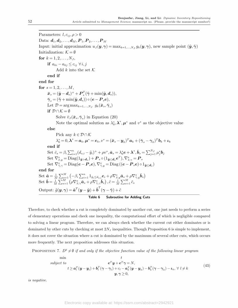
Benjaafar, Jiang, Li, and Li: Dynamic Inventory Repositioning
52 Article submitted to Management Science; manuscript no. (Please, provide the manuscript number!)
Parameters: l, cij, ρ > 0
Data: d1,d2, . . . ,dM ,P 1,P 2, . . . ,PM
Input: initial approximation uJ(y,γ) = maxk=1,...,NJ gk(y,γ), new sample point (y, γ)
Initialization: K= ∅for k= 1,2, . . . ,NJ ,
if aki− akj ≤ cij ∀ i, jAdd k into the set K
end if
end for
for s= 1,2, . . . ,M ,
xs = (y−ds)+ +P Ts (γ+ min(y,ds)),
γs = (γ+ min(y,ds)) (e−P se),
Let D= arg maxk=1,...,NJ gk(xs, γs)
if D∩K= ∅Solve vJ(xs, γs) in Equation (20)
Note the optimal solution as λ∗0,λ∗,µ∗ and v∗ as the objective value
else
Pick any k ∈D∩Kλ∗0 = 0,λ∗ = ak,µ
∗ = ek, v∗ = (xs−yk)Tak + (γs−γk)Tbk + ιk
end if
Set cs = βi∑n
i=1(ds,i− yi)+ + ρv∗, as = λ∗0e+λ∗, bs =∑NJ
j=1 µ∗jbj
Set ∇sx,y = Diag(1y>ds) +P s (1y≤dseT ),∇sx,γ =P s
Set ∇sγ,γ = Diag(e−P se),∇sγ,y = Diag ((e−P se) 1y≤ds)
end for
Set a= 1M
∑M
s=1
(−βi
∑n
i=1 1yi≤ds,iei + ρ∇sx,yas + ρ∇sγ,ybs)
Set b= 1M
∑M
s=1
(ρ∇sx,γas + ρ∇sγ,γ bs
), c= 1
M
∑M
s=1 cs
Output: g(y,γ) = aT (y− y) + bT
(γ− γ) + c
Table 6 Subroutine for Adding Cuts
Therefore, to check whether a cut is completely dominated by another cut, one just needs to perform a series
of elementary operations and check one inequality, the computational effort of which is negligible compared
to solving a linear program. Therefore, we can always check whether the current cut either dominates or is
dominated by other cuts by checking at most 2NJ inequalities. Though Proposition 6 is simple to implement,
it does not cover the situation where a cut is dominated by the maximum of several other cuts, which occurs
more frequently. The next proposition addresses this situation.
Proposition 7. Dk 6= ∅ if and only if the objective function value of the following linear program
min t
subject to eTy+ eTγ =N,
t≥ aTl (y−yl) + bTl (γ−γl) + cl−aTk (y−yk)− bTk (γ−γk)− ιk, ∀ l 6= k
y,γ ≥ 0,
(43)
is negative.
Electronic copy available at: https://ssrn.com/abstract=2942921
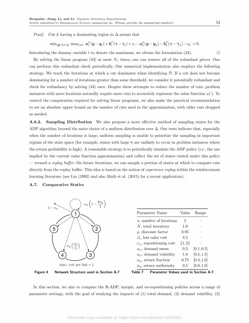
Benjaafar, Jiang, Li, and Li: Dynamic Inventory Repositioning
Article submitted to Management Science; manuscript no. (Please, provide the manuscript number!) 53
Proof. Cut k having a dominating region in ∆ means that
min(y,γ)∈∆ maxl 6=k aTl (y−yl) + bTl (γ−γl) + cl−aTk (y−yk)− bTk (γ−γk)− ιk < 0.
Introducing the dummy variable t to denote the maximum, we obtain the formulation (43).
By solving the linear program (43) at most NJ times, one can remove all of the redundant pieces. One
can perform this redundant check periodically. Our numerical implementation also employs the following
strategy. We track the iterations at which a cut dominates when identifying D. If a cut does not become
dominating for a number of iterations greater than some threshold, we consider it potentially redundant and
check for redundancy by solving (43) once. Despite these attempts to reduce the number of cuts, problem
instances with more locations naturally require more cuts to accurately represent the value function u(·). To
control the computation required for solving linear programs, we also make the practical recommendation
to set an absolute upper bound on the number of cuts used in the approximation, with older cuts dropped
as needed.
A.6.2. Sampling Distribution We also propose a more effective method of sampling states for the
ADP algorithm beyond the naive choice of a uniform distribution over ∆. Our tests indicate that, especially
when the number of locations is large, uniform sampling is unable to prioritize the sampling in important
regions of the state space (for example, states with large γ are unlikely to occur in problem instances where
the return probability is high). A reasonable strategy is to periodically simulate the ADP policy (i.e., the one
implied by the current value function approximation) and collect the set of states visited under this policy
— termed a replay buffer. On future iterations, we can sample a portion of states at which to compute cuts
directly from the replay buffer. This idea is based on the notion of experience replay within the reinforcement
learning literature (see Lin (1992) and also Mnih et al. (2015) for a recent application).
A.7. Comparative Statics
1
2
34
5
repo. cost per link = 1
αp
(αq
5
)
αp
(1− 4αq
5
)
1− αp
Figure 4 Network Structure used in Section A.7
Parameter Name Value Range
n, number of locations 5 –
N , total inventory 1.0 –
ρ, discount factor 0.95 –
βi, lost sales cost 4.5 –
cij , repositioning cost 1,2 –
αν , demand mean 0.3 [0.1,0.5]
ασ, demand volatility 1.0 [0.5,1.5]
αp, return fraction 0.75 [0.4,1.0]
αq, return uniformity 0.5 [0.0,1.0]
Table 7 Parameter Values used in Section A.7
In this section, we aim to compare the R-ADP, myopic, and no-repositioning policies across a range of
parameter settings, with the goal of studying the impacts of (1) total demand, (2) demand volatility, (3)
Electronic copy available at: https://ssrn.com/abstract=2942921

Benjaafar, Jiang, Li, and Li: Dynamic Inventory Repositioning
54 Article submitted to Management Science; manuscript no. (Please, provide the manuscript number!)
return fraction (i.e., fraction of vehicles returned per period), and (4) uniformity of return locations. We
again use N = 1 and set ρ= 0.95. Due to the large number of MDP instances that we need to solve, we only
consider n= 5 locations, creating a set of 9-dimensional MDPs. Let νi = 0.2 for i= 1,2, . . . ,5 and we set the
mean demand at each location to be νi = αν νi for some scaling parameter αν , so that∑
iνi = αν . Similar
to before, we set σi = ασ νi for another scaling parameter ασ. The repositioning costs cij are illustrated in
Figure 4: the cost between adjacent locations is 1 and the cost between non-adjacent locations (e.g., 1 and
3 or 5 and 2) is 2. The return behavior is controlled by two parameters αp, the fraction of rented vehicles
returned (thus, 1−αp is the fraction of rented vehicles that remain rented), and αq, which we interpret as
the “return uniformity.” For αq = 1, returns are split evenly between the 5 locations and for αq = 0, vehicles
are returned to their rental origins. These two parameters are also illustrated in Figure 4 for location 1. We
vary each of the scaling parameters αν , ασ, αp, and αq individually; their nominal values and test ranges are
summarized in Table 7. In all solved instances, we use a maximum of 1,000 cuts in the approximation while
the ADP algorithm is run for 10,000 iterations17; all other algorithmic settings are as described in Section
6.3. The results are given in Figure 5. In each plot, lines illustrate absolute cost values of each policy for each
parameter setting (x-axis), while the bars illustrate the percentage decrease in cost achieved by the ADP
policy compared to the myopic and no-repositioning policies.
Figure 5 Impact of Parameters (Left-Axis & Bar: % Improvement of ADP; Right-Axis & Line: Raw Cost)
There are a few key takeaways from these experiments, which we now summarize. We see that when the
mean demand αν in the system is high (greater than 45% of the total inventory), the performance of the
17 As shown in the previous section, 10,000 iterations is enough to produce a near-optimal policy for n= 5.
Electronic copy available at: https://ssrn.com/abstract=2942921

Benjaafar, Jiang, Li, and Li: Dynamic Inventory Repositioning
Article submitted to Management Science; manuscript no. (Please, provide the manuscript number!) 55
myopic policy essentially matches that of the ADP policy. This can be explained by the observation that
lost sales in high demand systems are somewhat inevitable, so the impact of considering return behavior and
future cost is diminished. On the other hand, when demand is between 10% and 40% of the total inventory,
a substantial improvement of between 7%–40% beyond the myopic performance is observed. The largest
improvement, 40%, is seen for αν = 0.2. Demand volatility ασ has a strong influence on cost for all three
policies, with the cost of the ADP policy ranging from 0.54 for ασ = 0.5 and growing tenfold to 5.90 for
ασ = 1.5. We also observe that the gap between the ADP and myopic policies shrinks for higher volatility
systems.
The latter two plots are related to the return behavior parameters αp and αq. Although the cost decreases
when the return fraction αp increases (as there is more inventory with which to satisfy demand), the improve-
ment upon the myopic policy increases. Intuitively, given more available inventory due to fewer ongoing
rentals, the ADP policy has more “opportunities” to reposition and plan for future periods. We also see
that return uniformity αq tends to increase the cost under the ADP and myopic policies, but interestingly,
if no-repositioning is used, the cost is actually reduced as αq increases in the range of [0,0.6]. This can per-
haps be explained by the “natural repositioning” induced by the return behaviors, an effect that disappears
when active repositioning (i.e., ADP or myopic) is allowed. Similar to the case of demand volatility, the gap
between the ADP and myopic policy decreases as uniformity increases.
A.8. Details of the Clustering Approach Used in the CR-ADP Algorithm
Details of the clustering approach used in Section 7.1 are provided below.
• For simplicity, suppose that n is divisible by n. We take a geographical clustering approach18 and group
adjacent locations by setting Ck = (k− 1)n/n+ 1, . . . , kn/n.• We transform the demand by summing within clusters. For cluster k, we set dt,k =
∑i∈Ck
dt,i. Moreover,
we define “demand weights” χik that conceptually represent the weight of a particular location in a cluster
of locations. For each i∈ Ck, let χik = Edt,i/∑
j∈CkEdt,j .
• We keep the lost sales cost unchanged: βi = βi. For the repositioning cost from cluster k to cluster q, we
take an averaging approach:
ckq =1
|Ck|∑
i∈Ck
1
|Cq|∑
j∈Cq
cij
• The transformed return fraction from cluster k to cluster q is given by:
pt,kq =∑
i∈Ck
χik∑
j∈Cq
pt,ij ,
where we first sum over Cq and then take a weighted average over Ck using the weights χik defined above.
• Finally, for a location i in cluster k, we define our splitting heuristic to be: yi = χik yk.
18 Another conceivable approach is to group locations by demand (i.e., group many small locations together).
Electronic copy available at: https://ssrn.com/abstract=2942921
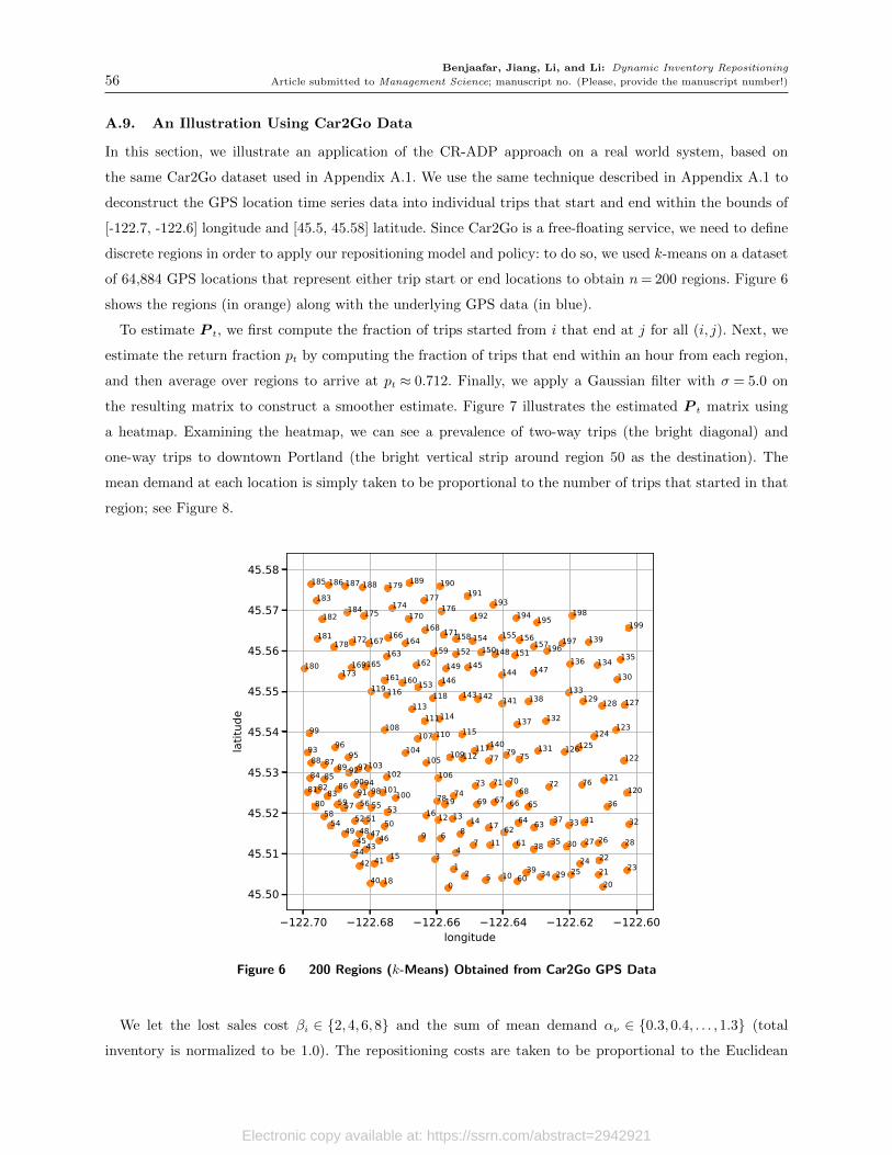
Benjaafar, Jiang, Li, and Li: Dynamic Inventory Repositioning
56 Article submitted to Management Science; manuscript no. (Please, provide the manuscript number!)
A.9. An Illustration Using Car2Go Data
In this section, we illustrate an application of the CR-ADP approach on a real world system, based on
the same Car2Go dataset used in Appendix A.1. We use the same technique described in Appendix A.1 to
deconstruct the GPS location time series data into individual trips that start and end within the bounds of
[-122.7, -122.6] longitude and [45.5, 45.58] latitude. Since Car2Go is a free-floating service, we need to define
discrete regions in order to apply our repositioning model and policy: to do so, we used k-means on a dataset
of 64,884 GPS locations that represent either trip start or end locations to obtain n= 200 regions. Figure 6
shows the regions (in orange) along with the underlying GPS data (in blue).
To estimate P t, we first compute the fraction of trips started from i that end at j for all (i, j). Next, we
estimate the return fraction pt by computing the fraction of trips that end within an hour from each region,
and then average over regions to arrive at pt ≈ 0.712. Finally, we apply a Gaussian filter with σ = 5.0 on
the resulting matrix to construct a smoother estimate. Figure 7 illustrates the estimated P t matrix using
a heatmap. Examining the heatmap, we can see a prevalence of two-way trips (the bright diagonal) and
one-way trips to downtown Portland (the bright vertical strip around region 50 as the destination). The
mean demand at each location is simply taken to be proportional to the number of trips that started in that
region; see Figure 8.
122.70 122.68 122.66 122.64 122.62 122.60longitude
45.50
45.51
45.52
45.53
45.54
45.55
45.56
45.57
45.58
latit
ude
98
75
174
33
154
0
130116
87
6147
19
182
124
153
115
2849
196
6859
171
835
155166
11
188
109
34
82
16
42
121
129
190
165
111
103
126
199
5
53
24
142
91
194
141
95
4
71
140
152
15
134
120
52
191
161
20
183
167
180
105
178
102
93
54 63
177
9
132
90
136151
89
22
40
48
60
26
65
1
66
150
100
6
117
108
14
168
122
32
110
179
7684
195
149
187
25
7
147
38 27
106
198
41
55
157
146
131
123
144
96107
70
50
83
17
193
94
176
163
118
31
135
45
162
181
175
85
74
138143
10
56
172
173
37
101
64
92112
12
30
113
139158
67
189
137
29
79
80 78
125104
72
160
21
13
133119
43
148
184
23
99
145
57
339
366958
164159
185
62
18
77
127
81
197
128
44
51
73
186
86
9788
169
156
192
46
170
114
2
Figure 6 200 Regions (k-Means) Obtained from Car2Go GPS Data
We let the lost sales cost βi ∈ 2,4,6,8 and the sum of mean demand αν ∈ 0.3,0.4, . . . ,1.3 (total
inventory is normalized to be 1.0). The repositioning costs are taken to be proportional to the Euclidean
Electronic copy available at: https://ssrn.com/abstract=2942921

Benjaafar, Jiang, Li, and Li: Dynamic Inventory Repositioning
Article submitted to Management Science; manuscript no. (Please, provide the manuscript number!) 57
0 25 50 75 100 125 150 175destination
0
25
50
75
100
125
150
175
orig
in
Figure 7 Heatmap of Estimated Transition P t
0 25 50 75 100 125 150 175 200location
0.000
0.005
0.010
0.015
0.020
norm
alize
d de
man
d
Figure 8 Normalized Demand Means
βi | αν 0.3 0.4 0.5 0.6 0.7 0.8 0.9 1 1.1 1.2 1.3
2 21.9% 36.2% 34.8% 54.0% 59.2% 67.0% 74.2% 79.3% 83.2% 86.1% 88.4%
4 18.4% 26.1% 32.7% 46.2% 62.9% 66.7% 73.7% 79.1% 83.0% 86.0% 88.2%
6 32.8% 28.7% 31.7% 47.2% 60.5% 67.4% 73.5% 79.0% 82.9% 85.9% 88.2%
8 17.9% 21.8% 33.0% 46.2% 66.2% 71.7% 73.7% 78.8% 82.8% 85.9% 88.2%
Table 8 Performance of CR-ADP as Percentage of the No-Repositioning Policy’s Cost (Lower is Better)
Electronic copy available at: https://ssrn.com/abstract=2942921

Benjaafar, Jiang, Li, and Li: Dynamic Inventory Repositioning
58 Article submitted to Management Science; manuscript no. (Please, provide the manuscript number!)
distance between regions, ranging between 0 and 1. The discount factor is assumed to be ρ = 0.99. Our
CR-ADP policy reduces the problem of 200 locations to a system with n = 10 clusters of equal size, with
cluster k containing regions 20(k − 1) + 1 to 20k, as labeled in Figure 6 (these are roughly grouped by
geographical location). R-ADP is run on the auxiliary MDP for 20,000 iterations and a policy for the n= 200
location case is then defined via the approach described in Section A.8. The results, relative to the cost of
the no-repositioning policy19, are shown in Table 8. We can see that CR-ADP produces significantly lower
costs in all instances. The largest relative improvements compared to no-repositioning are when the total
demand is low, consistent with what is shown in Figure 5.
19 The other policies are omitted due to the high computational cost of running them for n= 200.
Electronic copy available at: https://ssrn.com/abstract=2942921
Related Documents