Dynamic Interpretation of Emerging Systemic Risks Kathleen Weiss Hanley and Gerard Hoberg * Current version: September 15, 2016 ABSTRACT We use computational linguistics to analyze risk factors in bank 10-Ks to develop an empirical model of dynamic, interpretable emerging risks that is grounded in the theory of Gorton and Ordonez (2014) and that successfully predicts financial instability. The model detects risks in advance of the 2008 fi- nancial crisis as early as late 2005. Risks related to interest rates, mortgages, real estate, capital requirements, rating agencies and marketable securities became highly elevated during this pre-crisis period, with individual bank risk expo- sures strongly predicting the probability of bank failure and future stock return volatility. Tests using very recent data indicate a rise in market instability since 2014 related to risks associated with sources of funding, marketable securities, regulation risk, and credit default. Overall, our model reliably assesses both the build-up of systemic risk in the financial system and bank-specific exposures in a timely fashion. * Lehigh University and The University of Southern California Marshall School of Business, respectively. Hanley can be reached at [email protected]. Hoberg can be reached at [email protected]. We thank the National Science Foundation for generously funding this research (grant #1449578). We also thank Christopher Ball for providing extensive support regarding our use of the metaHeuristica software platform and advice on the computational linguistic methods. We also thank Allen Berger, Harry DeAngelo, Greg Duffee, Naveen Khanna, Tse-Chun Lin, Andrew Lo, Frank Olken, Raluca Roman, Maria Zemankova and seminar participants at Michigan State University, UC Davis, University of Georgia, and the University of South Carolina for excellent comments and suggestions.

Welcome message from author
This document is posted to help you gain knowledge. Please leave a comment to let me know what you think about it! Share it to your friends and learn new things together.
Transcript
Dynamic Interpretation of Emerging Systemic Risks
Kathleen Weiss Hanley and Gerard Hoberg ∗
Current version: September 15, 2016
ABSTRACT
We use computational linguistics to analyze risk factors in bank 10-Ks to
develop an empirical model of dynamic, interpretable emerging risks that is
grounded in the theory of Gorton and Ordonez (2014) and that successfully
predicts financial instability. The model detects risks in advance of the 2008 fi-
nancial crisis as early as late 2005. Risks related to interest rates, mortgages, real
estate, capital requirements, rating agencies and marketable securities became
highly elevated during this pre-crisis period, with individual bank risk expo-
sures strongly predicting the probability of bank failure and future stock return
volatility. Tests using very recent data indicate a rise in market instability since
2014 related to risks associated with sources of funding, marketable securities,
regulation risk, and credit default. Overall, our model reliably assesses both the
build-up of systemic risk in the financial system and bank-specific exposures in
a timely fashion.
∗Lehigh University and The University of Southern California Marshall School of Business, respectively.Hanley can be reached at [email protected]. Hoberg can be reached at [email protected]. Wethank the National Science Foundation for generously funding this research (grant #1449578). We alsothank Christopher Ball for providing extensive support regarding our use of the metaHeuristica softwareplatform and advice on the computational linguistic methods. We also thank Allen Berger, Harry DeAngelo,Greg Duffee, Naveen Khanna, Tse-Chun Lin, Andrew Lo, Frank Olken, Raluca Roman, Maria Zemankovaand seminar participants at Michigan State University, UC Davis, University of Georgia, and the Universityof South Carolina for excellent comments and suggestions.

Banks may be the black holes of the financial universe; hugely powerful and influential, but tosome irreducible extent unfathomable.”
Morgan (2002)
I Introduction
Understanding the nature of information production in the banking industry is critical
to assessing whether financial instability is detectable and avoidable. Theories suggest
that the incentives, and ultimately the timing, surrounding information production are
nuanced. Information can be privately valuable to individual investors and depositors, but
significant ongoing informational opaqueness can be socially optimal. For example, Gorton
and Ordonez (2014) argue that the banking sector is more efficient when there is little or
no information production on the quality of bank assets, as this economizes on information
costs and, in so doing, leads to lower borrowing costs and greater economic growth. Yet
opaqueness that is optimal in normal times exposes the economy to periodic crises following
aggregate negative shocks to collateral values. Information production to ascertain collateral
quality will then increase for a period of time until the crisis is resolved.
Models in this area assume that there are only two states of nature: normal times when
there is no information generation, and crisis periods that induce information production.
However, the path from stability to crisis is clearly not instantaneous given real world
frictions. Slow information diffusion in asset pricing could be due, for example, to short
sale constraints (Diamond and Verrecchia (1987)), limits to arbitrage (Shleifer and Vishny
(1997)), information processing and awareness (Merton (1986)), and/or limited investor
attention (Barber and Odean (2007)). Practically speaking, we suggest that there exist
three states of information production: (1) no information production (normal period), (2)
some information production as systemic risk is building (transition period), and (3) high
information production (crisis period).
Although opacity may be useful in stimulating economic growth, existing regulation
limits opacity because regulators require banks to disclose highly aggregated risk exposures
in their annual 10-Ks. We conjecture that the initiation of information production and thus
the start of the transition period can be detected by examining the link between financial
market trading and the collective risks disclosed by financial institutions.1
1For example, Bui, Lin, and Lin (2016) find that short selling in bank stocks increased during the yearsleading up to the crisis and predicts bank outcomes. This provides support for the underlying assumptionthat trading by potential information producers occurs during our proposed transitional period.
1

We use computational linguistics to identify the presence of information production
regarding systemic risks, and also to identify the specific channels through which systemic
risks build. We focus these tools on bank stock price co-movements and their link to
banks’ disclosed verbal risk factors. If the transition period is sufficiently long, then specific
systemic risk channels can, in principle, be identified early when it is possible to still mitigate
the severity of financial instability. Our findings, based on the recent financial crisis, indicate
that information production slowly builds for about three years during the transition period
from stability to instability.
The use of qualitative information in the assessment of emerging risks is a complement
to the many quantitative measures that have been proposed to monitor financial stability.
Bisias, Flood, Lo, and Valavanis (2012) provide a survey of over 30 systemic risk metrics and
this list continues to grow. The large number of proposed methods to monitor the build-up
of systemic risk is related to the fact that there are many ways of defining systemic risk
in a complex financial system. Examples include liquidity mismatch (Brunnermeier, Gor-
ton, and Krishnamurthy (2014)), interconnectedness (Billio, Getmansky, Lo, and Pelizzon
(2012), Allen, Babus, and Carletti (2012) and Elliot, Golub, and Jackson (2014)), and mea-
sures of bank risk (Adrian and Brunnermeier (2016) and Acharya, Pedersen, Philippon,
and Richardson (2012)) to name only a few. In support of using many such measures,
Bisias, Flood, Lo, and Valavanis (2012) argue that “a robust framework for monitoring and
managing financial stability must incorporate both a diversity of perspectives and a contin-
uous process for re-evaluating the evolving structure of the financial system and adapting
systemic risk measures to these changes.”
These existing risk measures can be categorized as general or specific. General measures
include those based on financial market variables such as the correlation of stock returns,
VIX, or CDS spreads. Specific measures obtain from a theoretical understanding of how
systemic risk might manifest, for example, inadequate liquidity or under-capitalization. The
drawbacks of general measures are twofold. First, they do not provide information on the
economic determinants of systemic risks. Second, they often assume that the source of
increased systemic risk is known, and that it is uniform across crises.
We begin by developing a framework that formalizes the ideal properties that systemic
risk models should have. Our approach is cognizant of the fact that the financial system
is complex, difficult for any one researcher to fully understand, and is constantly evolving.
First, we suggest that the econometric model should be automated, replicable, and free
2

from any bias imposed by the researcher. Second, the model must identify a set of emerging
systemic risk channels that are clearly interpretable. Third, the model must be dynamic, and
thus capable of identifying emerging risks that might not have been present in past periods
or that might not be anticipated. Fourth, the methodology should be flexible enough to
permit optional researcher exploration without loss of generality. Finally, the model must
identify emerging risks in a timely fashion and with adequate power to eventually allow for
regulatory intervention. As we argue below, each of these criteria are present in our model.
We propose that risk assessment of the disclosures of financial firms can provide valuable
information on both the intensity and source of emerging systemic risks. Textual analysis us-
ing 10-Ks is well-suited to the task as firms are required to disclose a synopsis of risks facing
the company.2 For example, these include discussions of interest rate risk (“In a sustained
rising interest rate environment the asset yields may not match rising funding costs, which
may negatively impact interest margins.”), capital adequacy (“ Republic’s failure to main-
tain the status of “well-capitalized” under our regulatory framework, or “well-managed”
under regulatory exam procedures, or regulatory violations, could compromise our status
as a FHC and related eligibility for a streamlined review process for acquisition proposals
and limit financial product diversification.”) and mortgage loan risk (“Our interest-only
mortgage loans may have a higher risk of default than our fully-amortizing mortgage loans
and, therefore, may be considered less valuable than other types of mortgage loans in the
sales and securitization process.”).3
We identify the list of potential systemic risks from 10-K text by extracting all text in
sections or subsections of the 10-K that have the root word “risk.” We use two text analytic
tools in tandem: Latent Dirichlet Allocation (LDA), a dimensionality reduction algorithm,
and Semantic Vector Analysis (SVA), which ensures interpretability while allowing for flex-
ibility and standardization. A drawback of LDA, if used alone, is that it is not always
interpretable and it produces a unique set of topics in each year making it difficult to track
the evolution of individual risks through time. Therefore, we use SVA in a second stage to
ensure interpretability and to standardize themes from LDA into a simple panel database
containing bank-year observations of each risk exposure. This approach allows us to lock
2After 2005, the SEC requires a separate risk factors disclosure section, Item 1A. Prior to this time, thesedisclosures were made in different sections throughout the 10-K.
3Text analytics in finance is growing in popularity and has been shown to explain asset prices andcorporate decisions in a variety of settings. For example, see Tetlock (2007), Tetlock, Saar-Tsechanksy, andMacskassy (2008), Tetlock (2010), Hanley and Hoberg (2010), Loughran and McDonald (2011), Hanley andHoberg (2012), Loughran and McDonald (2014), Hoberg and Maksimovic (2015), and Hoberg and Phillips(2016).
3

in some risk factors that are stable through time while allowing flexibility for the model to
detect newly emerging risks in any given period in our sample.
To identify the potential for systemic risk to emerge, we compute a pairwise covariance
matrix based on daily stock return comovement in each quarter from 1998 to 2015. To
determine which semantic risk themes are emerging in a given quarter, we examine the
link between pairwise covariances and common bank-pair exposures to each verbal risk
theme. We predict that return covariance will be significantly associated with common risk
exposures, but only in transition periods where systemic risk is building.
In order to assess whether a specific systemic risk emerges in the time-series leading
up to the financial crisis, we first estimate the adjusted R2 contribution of each of our 18
baseline candidate risks in explaining return covariance over the entire time series. We
then standardize the resulting quarterly time series from 2004 to 2015 by the mean and
standard deviation from a non-crisis baseline period (1998 to 2003). The resulting t-statistic
indicates whether the contribution of a specific theme is statistically significant and provides
an indication of importance. In addition, we also create an aggregate emerging risk score
as the R2 due to the contribution of all semantic themes in explaining return covariance.4
Our aggregate emerging risks score is shown in Figure 1. It becomes highly significant
(t-statistic above 8.0) in the second quarter of 2005, far in advance of the financial crisis. It
more than doubles to a level with a t-statistic exceeding 13.0 by the fourth quarter of 2006.
Other indicators of systemic risk such as VIX or aggregate measures of volatility do not
become significantly elevated until the crisis begins in 2008. We also note that our aggregate
systemic risk score does not become elevated during other episodes of market volatility that
were not ultimately systemic in nature for banks specifically. For example, the bursting of
the technology bubble of 2000 and the events surrounding 9/11/2001 were both associated
with volatile stock returns, but there were no serious spillovers to financial intermediaries
and no threats to financial stability. We view these events as falsification tests. That is, our
model does not produce elevated systemic risk themes simply when markets are volatile.
Rather, our model is designed to measure systemic risks and to assess financial stability.
We next examine the specific types of risks that emerged in the lead-up to the financial
crisis. We show that themes related to interest rates and mortgages (Mian and Sufi (2009)),
rating agencies (White (2010)), dividends (Acharya, Gujral, Kulkarni, and Shin (2011)), risk
4Gao (2016) finds that including a text-based systematic risk factor into a four-factor Fama-French modelincreases R2 and the factor is associated with a positive risk premium.
4

management (Aebia, Sabatob, and Schmid (2012)) and marketable securities rise in their
ability to explain bank-pair return covariance as early as 2005.
Because our methodology allows for flexibility in the examination of risks, we further
consider sub-themes known to be related to increased risk during the financial crisis. For ex-
ample, sub-themes within the broader category of marketable securities include commercial
paper (Covitz, Liang, and Suarez (2013)), cash (Cornett, McNutt, Strahan, and Tehranian
(2011)), mortgage-backed securities (He, Qian, and Strahan (2011)), and municipal bonds
(Dwyer and Tkac (2009)). We show a heightened impact of each of these sub-themes on
bank-pair covariance in the period leading up to the crisis, especially mortgage-backed se-
curities and commercial paper, indicating an early understanding (as early as late 2005) by
investors that risks associated with these asset classes were of concern. Thus, our method
can provide regulators with an early warning of specific emerging risks that might affect
financial stability.
The aforementioned results are based on aggregate time series analysis. Our framework
also enables us to measure the exposure of specific banks to systemic risk in the cross-
section. We examine whether institution level exposure predicts subsequent stock returns,
volatility and bank failures. We find that the more a bank is exposed to emerging risk
factors from early 2006 until the second quarter of 2008, the greater is the negative return
during the financial crisis from September 2008 to December 2012.
We analyze whether our methodology can predict subsequent bank failures. Using data
on bank failures from the FDIC, we show that banks exposed to more emerging risk factors,
as early as the beginning of 2006, are more likely to fail during the 2008 financial crisis and
its aftermath.
Last, to assess the impact of emerging risk factors in the cross-section more generally,
we use Fama and MacBeth (1973) regressions where the dependent variable is an ex post
monthly stock return volatility and the independent variable of interest is the emerging
risk exposure of each financial firm measured over one, two, three and four quarters. We
find that both recent and deeply lagged exposures (up to 30 months) predict subsequent
monthly volatility.
Collectively, our results indicate that text analytics can identify emerging risks and
detailed semantic analysis can reveal the underlying mechanisms driving these risks that can
be useful to researchers and regulators interested in assessing financial stability. Moreover,
5

this might be possible years before systemic risks reach crisis levels.
Up to this point, our analysis has focused on historical events. But in order for our
methodology to prove its dynamic properties, it must also provide insights regarding emerg-
ing risks in the future. Examining emerging risk factors in very recent data (through the
beginning of 2016) indicates a substantial build-up of potential systemic risk at present.5
Concerns about sources of funding, marketable securities, credit default, regulation risk,
and capital requirements are examples of the risks we see emerge starting in early 2014.
More importantly, we show that financial firms’ exposure to these emerging risks predicts
bank-specific negative stock returns from December 2015 to February 2016 (when financial
firms were particularly volatile). While it is too early to tell whether a systemic event will
occur in the future, our findings suggest that researchers and regulators should be aware
about the potential impact of current emerging risks.
In addition to contributing to the research on systemic risk metrics and bank failures
(Sarkar and Sriram (2001), Cole and White (2011), Fahlenbrach, Prilmeier, and Stulz (2012)
and DeYoung and Torna (2013)), our paper is related to a growing literature on early
warning systems.6 Unlike many papers that propose metrics based upon variables known
to affect financial institutions during the financial crisis, our methodology is not predicated
on defining the source of systemic risk, and thus, does not suffer from a “post-crisis bias”
(Bussiere and Fratzscher (2006)). Because of substantial reforms in the financial sector, the
risks that emerge in the next crisis are unlikely to resemble those from previous financial
crises. Our methodology is dynamic and free of researcher bias. Hence it allows for the
identification even of emerging risks for which researchers or regulators have no ex-ante
knowledge.
II Existing Theory and Motivation
We briefly explain how our paper is motivated directly from theories of systemic risk in
the banking sector. Although we discuss specific theories of bank opacity below, we also
note the presence of a broader literature that examines the impact of mandated disclo-
sures on financial market regulation.7 Our findings contribute to the debate of whether
5As with all predictive models, this is a joint test of the significance of the risks in the economy and thesignificance of the model to predict those risks.
6See for example, Huang, Zhou, and Zhu (2009), Giesecke and Kim (2011), Estrella and Mishkin (2016),Frankel and Saravelos (2012), and Duca and Peltonen (2013).
7See Verrecchia (2001), Dye (2001), Healy and Palepu (2001), and Beyer, Cohen, Lys, and Walther (2010)for additional reviews of the literature on collective disclosures and the informational environment.
6

enhanced financial disclosure is beneficial from the perspective of societal welfare (Kurlat
and Veldkamp (2015)).
Early papers such as Diamond and Dybvig (1983) and Gorton and Pennacchi (1990)
and more recently, Gorton and Ordonez (2014) and Dang, Gorton, Holstrom, and Ordonez
(2016), suggest that the banking sector (or debt more broadly) generates the most value
to society when there is no information production specific to underlying loans. Bank
opacity avoids scenarios where banks issue sub-optimally small loans to avoid incentivizing
information production, and allows uninformed investors to participate without paying
information rents.8 In turn, this reduces borrowing costs and increases economic growth.
Other papers theorize that opacity can create financial stability and contagion. Bouvard,
Chaigneau, and Motta (2016) examine the interaction between opacity and the voluntary
disclosure of private information of regulators. In this case, opacity signals good news
because regulators will only disclose information in times of crisis.9 Thus, markets appear
to know some but not all of the relevant information about the risks facing banks. This
creates under-reporting of information because the regulator makes the system opaque in
more states than is optimal, creating instability. Alvarez and Barlevy (2015) agree that bank
opacity can, at times, be optimal for bank risk sharing. However, if contagion is severe,
requiring banks to disclose more information can improve welfare. Begley, Purnanandam,
and Zheng (2016) show that banks under-report their market risks when they have incentives
to save equity capital, and this coincides with periods of systemic risk.
Thus, the literature suggests that bank opacity can expose society to financial crises as
an absence of information production can allow systemic risk to build unchecked, creating
large panics ex post. This raises the question as to whether it is possible to enjoy an optimal
level of bank opacity, and yet establish a mechanism for reducing crisis risk.
The benefits of bank opacity may be feasible to maintain if information produced about
financial instability has the following three traits: (1) such information can be generated
8Whether banks are indeed opaque is subject to debate. Flannery, Kwan, and Nimalendran (2013) ex-amine opacity using market trading patterns of banks. During normal times, larger banks do not appear tobe more opaque than their non-financial control firms. However, during the crisis period, banks’ microstruc-ture diverges from non-banks, which increases opacity. Jeffrey S. Jones and Yeager (2013) find that bankinvestments in opaque assets create more systematic risk and increase price synchronicity.
9Peristian, Morgan, and Savino (2010) provide evidence on the release of stress test results and find thatthe market can distinguish between banks that did and did not have a capital gap before the stress test.They document a market reaction upon announcement only for banks with a capital gap and conclude that“the stress test produced information about the banks that private sector analysts did not already know.”The fact that investors knew some of the risks facing banks, but not all, is a key requirement for a prolongedtransition period leading up to crisis periods.
7

at little to no cost (Andolfatto, Berentsen, and Waller (2014)), (2) it is uninformative in
normal times, and (3) it is uninformative about specific loan attributes. The ability to
produce information having these traits is especially beneficial if the costs to society of
large scale panics is high, and if preemptive regulatory interventions can potentially reduce
the severity of impending crises.
The information generated by our risk model generally satisfies these three criteria.
First, because it is automated, information gathering costs are negligible. Second, the
model is designed to produce no information about individual loans or assets, and it is
also designed to produce no information in normal times. That is, the model is designed to
produce aggregate information about systemic risk, and only when systemic risk is building.
These unique properties are made possible because we focus only on co-movement in returns
that might plausibly be driven by candidate emerging systemic risk factors, which are not
specific to any particular asset.
The empirical framework adopted in our paper is motivated by the aforementioned
theory that suggests that in normal times investors will not find it profitable to produce in-
formation. As financial instability increases, investors will invest in information production
regarding the risks facing banks and will begin to trade on this information. If investors
are trading on specific emerging risks, the key prediction is that pairs of banks exposed
to the same risk will experience aberrational co-movement. This will, in turn, create el-
evated return covariance for bank pairs exposed to the same emerging risks allowing our
methodology to predict the potential for financial instability.
The benefits of such an emerging risk model are highest if the social planner can be
made aware of emerging risks before they reach crisis levels. This would allow the social
planner to fix the systemic flaws through regulatory change, which would then allow the
economy to return to normal times without a full-fledged panic. Thus, in order for our
methodology to be useful for researchers and policymakers, it must identify emerging risks
in a dynamic, flexible and comprehensive manner even in changing market conditions. We
propose that an ideal model should satisfy the following five requirements:
Requirement 1 (Bias-Free): The model should be automated, replicable, and fast
to execute. Non-automated approaches are likely intractable given the large volume of
verbal risk factor data disclosed in 10-Ks. In addition, the method should not require user
input as to the selection of the emerging topics.
8

Requirement 2 (Interpretable): The output from the model must produce a set of
emerging risk factors that are clearly interpretable without ambiguity. Empirical research
requires that identification of specific textual themes should be easily interpretable in order
to measure their impact. Precision in isolating the type of emerging risk is particularly
critical when considering policy interventions.
Requirement 3 (Dynamic): The model must be dynamic, and capable of identify-
ing emerging risks in the current period that might not have been present in past periods.
Generally, empirical asset pricing focuses on stable risk factors. In contrast, systemic risks
are by nature unique, and they can be spontaneous in nature. This requirement is partic-
ularly relevant when specific emerging systemic risks might not be ex ante known to the
researcher.
Requirement 4 (Flexible): Although the model should be capable of identifying
emerging risk factors without any researcher input (per Requirement 1), the model should
nevertheless allow the user to delve more deeply into the sources of risk using their knowledge
of current economic conditions. An ideal model will permit deeper analysis without loss of
generality.
Requirement 5 (Timely): The model must be able to detect emerging risks well in
advance of a systemic event. In order for the model to be useful for regulatory intervention,
the model must provide an early warning sign of areas of concern.
These requirements set a high bar, which cannot be met using many standard compu-
tational linguistic methods. For example, many studies use fixed vocabulary lists to score
documents (see Loughran and McDonald (2011) and Tetlock (2007) for example). This ap-
proach is useful in addressing many existing questions in the literature, and is automated.
However, the approach does not satisfy the bias free component of Requirement 1 in our
setting because the researcher must provide the word lists. The approach also is not dy-
namic (Requirement 3) because it offers no guidance regarding how the word lists might
change over time.
Given Requirement 1 in particular, the most suitable tools should be those that are
automated and that create content organically. Support vector regression (SVR) is an
example of a text analytic method used in the finance and accounting literature (Manela and
Moreira (2016) and Frankel, Jennings, and Lee (2016)) that does not require researcher input
regarding content. However, this method does not satisfy the rather critical Requirement
9

2 of interpretability. SVR only identifies single words or commongrams, and the results
are difficult to interpret. For example, Hoberg (2016) shows that SVR words tend to be
common words, words with multiple interpretations, and shorter words.
Latent Dirichlet Allocation (LDA), like SVR, also generates content automatically with-
out researcher bias. However, because the focus of LDA is on identifying specific topics
based on clusters of vocabulary, the algorithm comes closer to identifying links that are
interpretable. LDA is also fully automated and can be rerun in any period, making it dy-
namic as well. However, one drawback to this approach lies in the dynamic continuity of
LDA models. Because LDA regenerates themes in each time period, there is no thematic
continuity year-to-year, making it difficult to identify exposure to consistent themes over
time. In addition, the LDA algorithm is not flexible as it does not accept researcher input
beyond simple parameter specifications, and hence it does not satisfy Requirement 4.
As a result of these challenges, we consider a model of emerging risks that uses two
tools in tandem. The approach first runs LDA on the risk factor corpus to identify a set
of themes in each year. The model then uses Semantic Vector Analysis (SVA) to generate
fully interpretable output and to provide year-over-year continuity of common themes. The
pairing of these tools generates a model of semantic themes that can identify plausible
emerging risks in a timely fashion (Requirement 5) thus, satisfying all five requirements.
We now discuss how we implement our methodology using LDA and SVA .
III Methodology
We consider the corpus of verbal risk factors disclosed by U.S. banks in their 10-Ks from
1997 to 2014.10 In its raw form, the text is in paragraph form and is very high-dimensional
(many thousands of paragraphs and unique words). This complexity precludes using the
corpus to detect interpretable emerging risk factors without some dimensionality reduction.
We consider two text analytic tools to address this problem. The first, Latent Dirichlet
Allocation (LDA), is a dimensionality reduction algorithm. The second is Semantic Vector
Analysis (SVA), which ensures flexibility and direct interpretation of emerging risks.
10Following convention, we only use the initial 10-K filed in each fiscal year, and do not consider amended10-Ks which can be filed at a much later time.
10

A Extracting 10-K Risk Factors
Our sample of 10-K’s is extracted by web-crawling the Edgar database for all filings that
appear as “10-K,” “10-K405,” “10-KSB,” or “10-KSB40.” The document is processed for
text information, fiscal year, and the central index key (CIK). Although all of the text-
extraction steps outlined in this paper can be programmed using familiar languages and
web-crawling techniques, we utilize text processing software provided by meta Heuristica
LLC. The advantage of doing so is that the technology contains pre-built modules for fast
and highly flexible querying, while also providing direct access to analytics including Latent
Dirichlet Allocation and Semantic Vector Analysis (discussed in the next section).11 We
use all available fiscal years in the metaHeuristica database from 1997 to 2014.
One benefit of using metaHeuristica is that the discussion of risk factors in the 10-K
are time consuming to extract using standard programming methods. Starting in 2005,
risk factors became more standardly placed in Item 1A. Prior to 2005, however, most firms
discussed risk factors in many different parts of the 10-K with heterogeneous subsection
labels. metaHeuristica’s dynamic querying tools allow us to identify and query directly
sections and subsections of the 10-K containing the word root “risk” regardless of where
they are in the 10-K.
The output from these metaHeuristica queries is the full set of paragraphs that contain
discussions of risk factors for all banks in our sample in all years from 1997 to 2014. Each
paragraph is linked to key identifiers including the bank’s central index key (CIK), the file
date of the given 10-K, the bank’s fiscal year end, and the filer’s SIC code. This database
of paragraphs is the central input to the text analytic methods we discuss.
B Latent Dirichlet Allocation
LDA is a dimensionality-reducing algorithm used extensively in computational linguistics
that was developed by Blei, Ng, and Jordan (2003). The method was created from an
underlying model in which each document is assumed to be generated from a probability
distribution over topics. Suppose there are T topics that a document writer might choose
from. The vocabulary corresponding to each topic, when written, is assumed to be generated
using a distribution of vocabulary associated with an individual topic. LDA algorithmically
11For interested readers, the metaHeuristica implementation employs “Chained Context Discovery” (SeeCimiano (2010) for details). The database supports advanced querying including contextual searches, prox-imity searching, multi-variant phrase queries, and clustering.
11

derives both a measure of how much text in each document corresponds to each topic, and
the topic vocabularies for each topic.12
Each LDA topic is defined as a probability distribution over 100 individual words and 100
commongrams. For example, the word “mortgage” might occur with a higher probability
in a discussion of financing risk than in a discussion of internal risk management. Suppose
that there are a fixed number of T such topics that banks draw upon when writing their
risk factors (RFs). Potential topics might include interest rate risk, deposit risk, and risks
relating to sources of funding. When writing the 10-K and discussing risk factors, LDA
assumes that managers draw words from topic-specific vocabularies. Although readers of
10-Ks might expect specific risk factors to appear as topics, LDA does not require the user
to specify any topics ex ante. They are determined algorithmically by LDA using likelihood
analysis. This fact is critical to our requirements, as it implies that the algorithms can
detect an emerging risk even if the user is entirely unaware of the existence of the risk.
LDA requires only one decision from the user, i.e. the number of topics T to be gen-
erated. To maintain parsimony, in this study, we focus on 25 topics (although we consider
50 topics for robustness and find similar results). The choice of 25 topics reflects the
multi-faceted nature of RF text and allows us to identify higher-dimensional topics without
significant overlap.
LDA output is in the form of two data structures. The first data structure describes the
distribution of topics discussed by each bank in each year of our sample. These firm-year
specific distributions are commonly referred to as “topic loadings”. LDA generates a vector
of length 25 for each firm-year in our sample, scoring the document based on the extent
to which it discusses each of the 25 topics. This data structure is a reduced dimension
summary of the aggregate content of the RFs discussed throughout the 10-K. Raw 10-Ks
have a dimensionality exceeding 100,000, on average, corresponding to the number of unique
words. The output of LDA summarizes each document using vectors of length of 25.
The second data structure is a set of word frequency probabilities for each topic. For
LDA based on 25 topics, this data structure contains 25 individual word lists with corre-
sponding word probabilities. In other words, each topic is described as a vector of proba-
bilities of individual words. The word lists associated with each topic can be evaluated to
12We provide only a summary level discussion of LDA here. We refer more advanced readers interestedmethods to the original study by Blei, Ng, and Jordan (2003) for a complete treatment, or to the AppendixA in Ball, Hoberg, and Maksimovic (2016) for a less technical treatment.
12

determine the most important risk factors that appear in the sample of banks in a given
year.
Figure 2 displays a summary of the output of an LDA model using our sample of banks
in 2006. Overall, we find the choice of 25 topics to be both parsimonious and informative.
The figure shows that bank risk factors contain many topics that imply sensible risk factors
being disclosed by banks. These include interest rate risk, economic conditions, mortgage
loan risk, regulation risk, fair value, and corporate governance. However, the quality of
an LDA model needs to be assessed more deeply by looking at the full vocabulary lists
associated with each topic. Only if each topic can be cleanly interpreted as having only one
meaning, would we declare success regarding the “clear interpretation” requirement that
we discussed earlier as an ideal property of a risk model.
For example, the risk topic labeled “r-10” in the summary Figure 2 suggests that it is
related to real estate loans. The list contains phrases such as “real estate,” “loan portfolio,”
and “commercial real estate”. This topic is an example of a highly interpretable emerging
risk, as it is straightforward to understand that this source of this risk is related to real
estate loans.
Not all of the topics in the time-series, however, are easily interpretable, and some tend
to blend themes. For example, the topic labeled “r-08” in the summary Figure 2 contains
phrases such as “fair value,” “interest rate risk,” and “financial instruments.” Although
any one of these items individually might indicate an interpretable risk factor, the blending
of these in one LDA topic suggests ambiguous content.13 Thus, we conclude that LDA only
partially succeeds in satisfying Requirement 2, interpretability.
Another limitation is that LDA creates a unique list of emerging risk factors in each
year, and each is related to the emerging risk factors in prior years in a different way, making
it difficult compare topics over time. In order to identify stable risk factors, the researcher
would need to manually assess the similarity of topics from year to year. Such an assessment
can lead to the introduction of researcher bias, violating Requirement 3.
The final limitation of LDA is that it fails to deliver flexibility (Requirement 5 above).
LDA, as a canned algorithm, and does not accept input regarding the types of risk factors
that a user might like to explore further. For example, upon reviewing the results in Figure
13A deeper dive into the complete word lists comprising this topic confirm this assertion. It containsadditional terms such as “rate risk,” “financial instruments,” “cash flows” and “hedge,” making its overallcategorization ambiguous.
13

2, a researcher might wish to further understand the properties of an individual sub-risk
such as ”commercial real estate” with more granularity. Because LDA does not address
this issue, we propose an extended formulation that satisfies all five requirements.
C Semantic Vector Analysis
We propose a second stage procedure using Semantic Vector Analysis (SVA) based on a
module provided in the metaHeuristica software package to address the aforementioned
limitations of LDA. The SVA algorithm draws upon research in the area of “Distributional
Semantics”, a probabilistic approach used to uncover the semantics of natural language.
The intuition for this approach is that ”a word is characterized by the company it keeps”
as popularized by linguist John Rupert Firth (1957).
The SVA algorithm first collects distributional information (on a per word or a per
phrase basis) from the 10-K and stores it in high-dimensional vectors. The vectors can then
be used as a representational framework to characterize how any given word or phrase is
semantically related to other words in the corpus. This step is done using neural networks
as in Mikolov, Chen, Corrado, and Dean (2013) and Mikolov, Sutskever, Chen, Corrado,
and Dean (2013). In particular, we use a two-layer neural network to learn the contextual
use of words. The algorithm learns contextual use by using features of the text to (A)
predict a single word given its immediate surround words and (B) predict the surrounding
words of a single word. This approach allows us to generate a more flexible, interpretable
mechanism to identify risk factors.
We use the first stage LDA results to extract a list of economically relevant risk factors by
reviewing the results of the LDA model in detail, both at the summary level (Figure 2) and
at the detailed level for the 25 topics. However, this step is not fully automated because
the user must prune the list of LDA phrases to eliminate any boilerplate or redundant
information. Although user input is required (which might violate Requirement 3), it is
a necessary condition to ensure interpretability of the results (Requirement 2). Also note
that the extent of human interaction in this case is limited to pruning a list of essential
terms, which likely poses a more modest level of bias compared to methods that require
researchers to propose such a list without any guidance.
Our examination of the LDA topics results in 18 themes14 and the SVA algorithm
14We originally identified 21 themes but reduced the number to 18 after noting that three were highlycorrelated with other themes and were vague in interpretation. We dropped themes related “Economic
14

converts each of the 18 themes into a vector of 100 words and commongrams that best
represent the given theme in the corpus. The resulting vectors are lists of words and
phrases, each accompanied by a cosine similarity indicating how strongly linked the given
word or phrase is to the semantic theme.
Table I we displays these “semantic vectors” for a sample of six of our baseline 18
semantic themes. For example, the first two columns illustrate that the “Mortgage Risk”
theme loads on the words including “mortgages”, “originated”, “FNMA”, “single family”
etc. Intuitively, these words would be expected to appear in a discussion about Mortgage
Risk. The theme “Derivative & Counterparty Risk” loads on phrases including four words
having the root “counterparty”, and also terms like “swaps”, “netting arrangements”, and
“exposure”.
In all, the word lists associated with each semantic theme, by design, are interpretable.
This is because the lists are designed to maximize the identification of effective synonyms
to the specified theme itself (the key input to SVA is a theme, expressed as a concise
phrase, such as “mortgage risk”). Hence, the algorithm directly satisfies the interpretability
Requirement 2. This approach also offers flexibility because the user can add any risk factors
to this list even if they did not appear visibly in the LDA topics (therefore, satisfying
Requirement 5, flexibility). Because the SVA algorithms are run every year, it is dynamic
and therefore, the method also satisfies Requirement 4.
D Linking LDA to SVA
Our last step is to map the LDA topic model data structures to the SVA themes in order to
determine an individual bank’s exposure to each emerging risk. This is done for each SVA
theme, one at a time, by computing the cosine similarity between each SVA theme and the
raw text corresponding to each bank’s total risk factor disclosure.
In particular, for each year t, suppose there are nikt unique words that are in the union
of firm i’s risk disclosure and theme k. We represent the risk factor disclosure for the firm
as a vector with nikt elements, which we denote Wi,t. Each element is populated by the
number of times firm i uses a given word in its risk factor disclosure in year t and the vector
is normalized to have a length of 1. For any word that appears in SVA theme k but not in
firm i’s risk disclosure, the element is set to zero. Analogously, we represent the vocabulary
Conditions”, “Board of Directors”, and “Products and Services”.
15

of theme k as a vector also with nikt elements, which we denote Tk,t. Each element of this
vector contains the numerical theme loadings as shown in Table I for words that are part
of the theme and this vector is also normalized to length 1. For any word that appears in
firm i’s risk disclosure but not in SVA theme k, the element is set to zero. Note that the
vectors Wi,t and Tk,t have the same length.
We thus compute firm i’s loading on semantic theme k in year t as Si,k,t as the normalized
cosine distance:
Si,k,t =Wi,t
||Wi,t||·Tk,t||Tk,t||
(1)
We compute the loading for firm i for each of the 18 semantic vectors. We thus have
a panel database with one observation being a single bank-year containing 18 semantic
theme loadings (Si,k,t∀k = 1, ...18).15 The resulting data structure allows us to observe the
intensity of every bank’s discussion of each of the 18 themes and how it changes over time.
A final note is that most of the 18 semantic theme loadings Si,l are not highly correlated
in the firm-year panel database. In particular, Table II reports the Pearson correlation
coefficients between each pair of loadings. The pairwise correlations are generally less than
40%. However, there are some exceptions as some pairwise correlations are in the 50% to
60% range. For example, there is a 66.7% correlation between capital requirements and
regulatory risk, and a 63.2% correlation between funding sources and capital requirements.
These correlations indicate that some risk factors tend to co-appear in the same bank
disclosures.
Despite some higher correlations, many banks still disclose one related theme without
disclosing the other, giving us power to separate the impact of each factor. To ensure
that multicollinearity is not affecting our results, we carefully inspect variance inflation
factors when we estimate our covariance regressions containing all 18 factors. Because these
regressions have a very large number of observations (the database is based on permutations
of all bank pairs and we have over 55 million bank-pair-quarter observations in total), our
ability to estimate variance inflation is high. We find that variance inflation factors never
exceed 3.5, well below the problematic threshold of 10 and conclude that multicollinearity
is not a first-order concern.
15Cosine similarity is bounded between 0 and 1 with observations closer to one indicating greater similaritybetween the SVA theme and the firm’s risk factor disclosure. Thus, if a particular SVA theme’s cosinesimilarity with firm i’s risk factor disclosure is close to one, this means that the bank’s discussion of thetheme is highly relevant and the opposite is true if the cosine similarity is close to zero.
16

IV Data and Sample
Our initial sample of publicly traded financial institutions are identified from the Center
for Research in Security Prices (CRSP) and Compustat databases as companies having SIC
codes in the range 6000-6199. To be included in our final database, a bank must also have a
link between its Compustat gvkey and its central index key (CIK), the unique identifier used
to track firms on the Edgar database provided by the Securities and Exchange Commission.
The gvkey to CIK links are obtained from the SEC Analytics database. Observations must
also have a machine readable discussion of risk factors in its 10-K as identified by the
metaHeuristica database. To satisfy this latter requirement, we query the metaHeuristica
database to find any 10-K section titles, or subsection titles, containing the word “risk” or
“risks”.
Our final sample contains 9,046 bank-year observations from 1997 to 2014 that satisfy
these requirements. We have an average of 503 publicly traded banks per year in our sample.
Figure 3 displays the composition of our sample over time. The figure shows that there are
483 banks in the first year of our sample, and the number of banks peaked in 1999 at 617
banks. One reason for this initial increase might be that banks did not consistently disclose
risk factors in the first two years of our sample, but more reliably disclosed risk factors after
1999. After the peak in 1999, the number of banks in our sample slowly declined to roughly
523 by the onset of the financial crisis in 2008 and further declined steeply to 315 by the
end of our sample in 2014. This reflects the well-known finding that many banks failed or
were acquired in the aftermath of the crisis.
A Financial Market Variables and Bank Characteristics
The literature on measurement of systemic risk often relies on financial market variables
to measure intertemporal changes in the financial stability of the economy. For example,
stock market returns capture common risk factors (Fama and French (1993)) that allow
for the identification of potentially systemic events in real-time using readily accessible
data (Brunnermeier and Oehmke (2013)). We consider stock market variables that either
capture the stock return co-movement among financial institutions, or that identify the
overall build-up of risk within the financial system. Our primary variable of interest is the
pairwise covariance based on daily returns from CRSP for pairs of financial firms in our
sample in a given quarter.
17
We then consider four additional measures to capture overall market risk or uncertainty.
The first measure is the cross-sectional standard deviation of monthly returns for all stocks
in the CRSP database in a given quarter. The second is an analogous measure based on
financial firms only. The third is the implied volatility of the European-style S&P 500 index
options (VIX). The fourth is the average pairwise covariance of banks in our sample.
Our primary measure of the informational relationship between banks is the pairwise
covariance for every permutation of bank i and j in every quarter t. We compute the
covariance using daily returns of bank pairs in each given quarter, and denote this as
Ci,j,t.16
We collect information from Call Reports on bank characteristics that have been used
in the literature (Cole and White (2011) and Cornett, McNutt, Strahan, and Tehranian
(2011)) as control variables in our covariance model. In addition, we also separately explore
the extent to which these accounting variables predict systemic risks. We aggregate Call
Report data at the holding company level if the bank has a parent ID, otherwise, data is
at the individual commercial bank level. In order to identify an identifier that can be used
to identify banks in our data, we merge the RSSD ID in the Call Report Data with the
New York Federal Reserves list of publicly listed institutions to obtain a CRSP PERMCO.
We use this field as a key to merge with our sample. If an institution does not have a Call
Report, we collect data on bank characteristics from COMPUSTAT.
Specifically, we construct the following variables (all but Assets are scaled by assets):
Cash and CatFat from Berger and Bouwman (2009) as measures of liquidity17, Loans and
Ln(Assets) as indicators of the size of the bank, Non-Performing Assets, the sum of loans
that are 30 days and 90 days past due and Loan Loss Prov & Allow, the sum of loan loss
provision and allowances to capture potential problem lending, Bank Holding Co. Dummy,
an indicator variable equal to one if the bank has a parent, zero otherwise, Neg. Earnings
Dummy an indicator variable equal to one if net income is negative, zero otherwise as a
measure of profitability, and Capital, the ratio of equity to assets as this measure has been
shown to predict subsequent bank performance (Berger and Bouwman (2013) and Cole and
White (2011)). Finally, we include Bank Age and it is constructed as the time since the
first appearance in CRSP.
16We winsorize these covariance estimates in each quarter at the 1/99% level to reduce the impact of anyoutliers.
17Generously provided by Christa Bouwman at https://sites.google.com/a/tamu.edu/bouwman/data.
18

We augment the database with Compustat industry data, which is based on SIC codes,
and with textual network (TNIC) industry data from Hoberg and Phillips (2016). Because
our framework naturally controls for industry as we limit our sample to banks, our additional
controls for TNIC are conservative, and allow us to control for additional variation in
product market offerings within the sample of banks (we also note that our results are robust
to excluding this step). Overall, the purpose of examining bank and industry characteristics
is to provide an array of control variables in our covariance regressions, as these variables
should explain a material amount of variation in bank-pair-quarter covariances. Hence, any
emerging risk factors we find can be seen as significant even relative to these existing drivers
of covariance.
B Summary Statistics
Table III displays summary statistics. Panel A reports statistics for bank-pair-quarter
variables. Because of the large number of permutations in this sample, there are over 55
million observations during our entire sample period. The Panel shows that the average
pair of banks, not surprisingly, has a high positive covariance. Because all of our sample
firms are financial institutions, 87.2% are in the same two-digit, 50% in the same three-digit
and 46.8% are in the same four-digit SIC code. The average TNIC pairwise similarity from
Hoberg and Phillips (2016) is 0.090, indicating a material amount of product similarity
among the banks in our sample. As a basis for comparison, the average pairwise similarity
of peer firms in the baseline TNIC network that is calibrated to be as granular as three
digit SIC is 0.064.
Panels B and C of Table III display summary statistics for the bank characteristics
that we consider. Most of the financial institutions in our sample, 85%, are bank holding
companies. The average bank has loans to assets of almost 50%. Loan loss provision
and allowances as well as non-performing assets are both close to zero (0.05% and 0.02%,
respectively). Most of the banks in our sample are bank holding companies and, on average,
have a capital ratio of 10%. Only 5% of banks have negative net income.
Panel D displays summary statistics for the quarterly time-series variables and we have
72 observations in our sample from 1997 to 2015. The average VIX index during our sample
is 21.2, and it reaches a high of 51.7 in the 4th quarter of 2008. The average cross sectional
standard deviation of monthly returns in our sample is 15.5% for all firms, and 9.1% for
banks only. The lower result for banks only is because (A) firms in a specific industry have
19

lower cross sectional variance due to the industry component being common to the included
firms and (B) banks are highly regulated and insured.
Although their construction is explained in the next section, we report the summary
statistics for two time series variables obtained from our emerging risk model. The first
is the average accounting variable (bank characteristics and industry ) adjusted R2, 7.7%,
indicating the explanatory power that standard bank characteristics and industry controls
have in explaining bank pairwise covariances. We also report the incremental R2, 0.8%, that
textual risk factors have in explaining pairwise covariance beyond the accounting controls.
Hence, the verbal risk factor metrics improve explanatory power by a material 10.4%. We
note that the accounting variable adjusted R2 has a higher R2 contribution because it is
well known that industry and firm characteristics, particularly size, are first-order drivers
of comovement.
Another observation from Panel C is that both R2 variables have substantial variation.
For example, the marginal R2 from the inclusion of verbal risk factors ranges between 0%
and 2.3%. This variation illustrates a crucial property of our emerging risk model: it can
detect time varying changes in the relationship between disclosed risk factors and bank pair
covariances.
Table IV displays Pearson correlation coefficients for our time series variables. The
standard time series variables used in past studies (VIX, cross sectional return volatility,
and average covariance) tend to be strongly, positively correlated. For example, the av-
erage pairwise covariance, and both metrics of average cross-sectional standard deviation
of monthly returns, are more than 50% correlated with the VIX. In contrast, the two R2
variables, text and accounting, from the risk model have lower and sometimes negative
correlations with the VIX and other volatility variables. This suggests that the measure
of systemic risk we propose is not highly correlated with other quantitative systemic risk
measures. Our later results will show that this is because our risk model R2 variables lead
these other measures in time series, reducing their simultaneous correlations.
V Determination of Emerging Risks
To determine which semantic risk themes are emerging or receding in a given quarter, we
examine the link between exposures to each risk theme and the monthly pairwise covariance
of banks i and j. Our central hypothesis is that stock return covariance, which is a measure
20

of co-movement of banks i and j, should become significantly associated with bank i and
bank j’s exposure to a given semantic risk theme if that specific risk is emerging. This
hypothesis relies on the assumption that a strictly positive number of investors are aware
of emerging risks, and trade on them, before they become prominent. If so, their aggregate
trading patterns will be detectable in the covariance data. Thus, banks jointly exposed to
a given risk factor should comove in a significant way in a given quarter.
The key independent variables we consider are the extent to which banks i and j are
exposed to the 18 semantic themes (Si,l and Sj,l ∀l = 1, ..., 18). Specifically, we take the
product of bank i and j’s loadings (cosine similarity) on each of the semantic themes S
(expressed here in vector form for all 18 risks):
Si,j = Si Sj (2)
The resulting pairwise semantic theme loadings capture the extent to which banks i and
j are exposed to the same emerging risks. We regress the quarterly return covariance of
banks i and j on each of these 18 semantic theme loadings and we also include controls for
industry, size, and accounting characteristics using the following is the regression equation:18
Covariancei,j,t = α0 + β1Si,j,t,1 + β2Si,j,t,2 + β3Si,j,t,3 + ...+ βTSi,j,t,18 + γXi,j,t + εi,j,t, (3)
This model produces 18 β coefficients for each of the 18 pairwise semantic theme load-
ings, and also a set of γ coefficients for industry and bank characteristics. These slopes are
computed separately in each quarter.
In the time series analysis that follows, we consider the R2 from the above regression
and decompose it into parts. First, we compute the R2 attributable to the industry and
accounting controls Xi,j,t by running the regression in equation (3) without the semantic
themes:
Covariancei,j,t = α0 + γXi,j,t + εi,j,t, (4)
Then we compute the marginal R2 that is attributable solely to the textual semantic
themes by taking the R2 from equation (3) and subtracting the R2 from equation (4).19 Note
that both R2 variables are now time-series variables, as each is derived from the regression
18We estimate pairwise control variables as the dot product of the variable for bank i with bank j.19For robustness, we also consider a variation where we use the 25 LDA topic loadings (Ti,j,t) instead
of the 18 semantic theme loadings (Si,j,t) and obtain similar results. This indicates that the 18 semanticthemes are correctly capturing information in the LDA loadings.
21

once per quarter. As a result, we are able to compare the time series properties of these R2
variables to standard financial market variables that are typically used to assess systemic
risk such as VIX or measures of aggregate volatility and comovement.
A Aggregate Time Series Results
We begin our analysis of whether our measures of emerging risk are informative in predicting
the build-up of systemic risk. We do so by comparing the time series R2 contribution
of the accounting and textual variables from our risk model in Equation 4 to the time
series variables that have been proposed as measures of systemic risk intensity. We define
the initial part of our sample (1998 to 2003) as a calibration period, and use this period
to compute each variable’s baseline quarterly mean and standard deviation. In each of
the subsequent quarters from 2004 to 2015, we compute a t-statistic based on how many
standard deviations the current value is from the baseline mean. A high t-statistic indicates
the likely presence of emerging risks.
We plot each variable’s time series of t-statistics in Figure 4, rather than reporting them
in tabular format, for ease of viewing. The benefit of the figure is that it makes it very clear
when each risk begins to emerge. In particular, we can see the relative importance of each
variable in the period leading up to the crisis and more recently.
Panel A of Figure 4 displays the time series of these t-statistics for four variables thought
to be indicative of systemic risk: the VIX, quarterly average pairwise covariance among
bank-pairs and the quarterly average standard deviations of returns for all firms and finan-
cial firms. Panel B plots the analogous time-series of t-statistics for the accounting and text
R2 variables used in our risk model. All variables are defined in Table III.
Examining the significance of financial market variables in Panel A, it is apparent that
the VIX, average covariance and both measures of cross sectional return volatility do not
become elevated above baseline levels until after Lehmann Brothers fails in September of
2008. We conclude that using these basic financial market variables as measures of emerging
risks, or as an early warning system, is problematic. This is because they do not become
prominent until the crisis has already emerged in full, too late to serve as an early warning
indicator.
When we consider the time series of t-statistics for the accounting variables in Panel B
of Figure 4, we find that it becomes different from the baseline period just after the first
22
quarter in 2007. From the end of the second quarter of 2007 through the first quarter of
2009, the R2 from accounting variables rises significantly above pre-crisis levels. Because
the financial market variables in Panel A do not emerge until late 2008, we conclude that
bank and industry characteristics are important in explaining variation in emerging risks,
and can be a leading indicator of financial instability.
More importantly, Panel B of Figure 4 shows that semantic themes emerge earlier than
both the financial market variables and the accounting variables used in the risk model. In
particular, the elevation of the textual semantic theme variables’ R2 becomes apparent as
early as late 2005 and strongly so by mid 2006. This is well before the crisis itself emerges,
and also before the accounting variables emerge. The semantic theme contribution remains
elevated as the crisis materializes in 2008, and tapers off as financial conditions begin to
improve.20
These preliminary results indicate that an aggregate measure of textual themes related
to risk can be an important ex ante indicator of emerging systemic risk. In the next section,
we examine the contribution of individual emerging risks to bank-pair covariance.
B Individual Emerging Risk Factor Time Series
The preceding analysis provides evidence that semantic themes that capture emerging risks
can provide an early warning of future periods of financial instability. A primary advantage
of sematic themes as a measure of emerging risk compared to accounting or financial market
variables is the ability to further interpret the text to identify the specific economic under-
pinnings of systemic risk build-up. Because accounting variables are low dimensional, they
cannot be interpreted with greater depth to identify specific manifestations. For example,
it is not clear what action should be taken to monitor systemic risk if firm size explains a
significant amount of comovement.
In this section, we examine the contribution of each specific semantic theme in explaining
how emerging risks affect the comovement of bank stocks. By doing so, we are able to
identify the content of specific emerging risks and when they begin to emerge.
As with the aggregate time series results in Figure 4, we first estimate the time series
of the marginal R2 contribution of each individual semantic theme in explaining pairwise
bank covariance using the model in Equation (3). This is done by computing the adjusted
20Using the R2 due to LDA topics rather than SVA themes results in a similar pattern. Thus, for theremainder of the paper, we concentrate on SVA textual themes.
23

R2 of the full model including all accounting variables and semantic themes, and then
recomputing the adjusted R2 with a single semantic variable excluded. This calculation is
done separately for each of the 18 semantic themes, and the result is a single quarterly time
series of R2 contributions for each semantic theme.
To generate a plot of statistical significance regarding each theme’s importance, we define
the initial part of our sample (1998 to 2003) as a calibration period, and use this period
to compute each semantic themes’ R2 baseline quarterly time series mean and standard
deviation. In each of the subsequent quarters from 2004 to 2015, we compute a t-statistic
based on how many standard deviations the current value is from the baseline mean. We
then plot the quarterly t-statistics for each semantic theme. We consider an increase in the
t-statistic to be indicative of an emerging risk factor.
Appendix A reports a fully detailed set of figures displaying the time series of t-statistics
for each of our 18 text-based emerging risk factors. In Figure 5, we restrict the presentation
to only the most prominent emerging risks in the period leading up to the 2008 financial
crisis. The figure shows large increases in the t-statistics for semantic themes related to
mortgages, real estate and interest rate risk, consistent with the build-up of risk in mortgage
credit in the period preceding the crisis (Mian and Sufi (2009)). Demyanyk and Hemert
(2011) suggest “that the seeds for the crisis were sown long before 2007, but detecting them
was complicated by high house price appreciation between 2003 and 2005 - appreciation
that masked the true riskiness of subprime mortgages.” Notably, our methodology detects
the emergence of these risks in 2005, well before delinquencies in the 2006 and 2007 loan
vintages became apparent.
We also observe elevated risks for marketable securities, indicative of worries by some
investors regarding the quality of these securities during the crisis. This finding is most
likely due to concerns about mortgage-backed securities and risks to the liquidity of various
short-term assets (Covitz, Liang, and Suarez (2013)).
We find that the semantic theme related to dividends is also prominent in the pre-crisis
period. Acharya, Gujral, Kulkarni, and Shin (2011) present evidence that banks, even
at the height of the financial crisis, continued to pay dividends to equity holders. The
paying of dividends further depletes regulatory capital at precisely the time as banks were
experiencing significant losses. The risk associated with the payment of dividends under
potentially adverse circumstances is reflected in the rise in the t-statistic for this theme
24

before the financial crisis.
It is well-known that credit rating agencies played a role in the crisis and we find an
emergence of this risk in early 2005 that dies down at the end of 2006 but becomes prominent
again in 2007. It re-emerges strongly before the Lehman bankruptcy in the first quarter of
2008. Our finding of a link to ratings supports the literature’s identification of problems
with the rating process such as ratings shopping (Benmelech and Dlugosz (2009), Skreta
and Veldkamp (2009), Bolton, Freixas, and Shapiro (2012), and Griffin and Tang (2012)),
ratings catering (Griffin, Nickerson, and Tang (2013)), rating agency competition (Becker
and Milbourn (2011)), and rating coarseness (Goel and Thakor (2015)).
The risk management theme is heightened as early as 2004 and remains elevated until
late 2007. This risk factor is less specific than those discussed above and likely captures
overall concerns about banks’ ability to manage increased exposure to systemic risk, and
the extent to which banks had robust risk management procedures in place. This theme is
important because the mitigation of risk is often discussed in conjunction with the disclosure
of such risks, making it a prominent leading indicator of the build-up of collective risks.
Finally, regulation risk begins to be elevated in late 2005 perhaps reflecting concern
about Federal Reserve intervention to chill an overheated housing market. In remarks to the
American Bankers Association Annual Convention on September 26, 2005, Chairman Alan
Greenspan expressed concern that the “apparent froth in housing markets may have spilled
over into mortgage markets.”21 Also note the significant increase in 2010 corresponding to
the passage of the Dodd-Frank Act.
Also noteworthy is that some risks do not appear to emerge around the 2008 crisis. In
Appendix A, we do not find elevated themes prior to the 2008 crisis related to credit default,
capital requirements, fair value, funding sources, bank deposits, or executive compensation
even though some of these risks were identified as contributing to the crisis ex post. For ex-
ample, concerns about executive compensation were raised, suggesting that bank managers
might have engaged in excessive risk taking because federal deposit insurance provides a
hedge against downside risk. Alan Blinder “refer(s) to the perverse incentives built into the
compensation plans of many financial firms, incentives that encourage excessive risk-taking
with OPM – Other People’s Money.”22
21http://www.federalreserve.gov/boardDocs/Speeches/2005/200509262/default.htm22Crazy Compensation and the Crisis, Wall Street Journal, May 28, 2009 http://www.wsj.com/articles/
SB124346974150760597. Note that Fahlenbrach and Stulz (2011) do not find evidence that worse compen-sation incentives were correlated with bank performance during the crisis.
25

Derivative and counterparty risk is only slightly elevated prior to the crisis despite the
fact that counterparty risk associated with credit default swaps might have enabled an
“unsustainable credit boom” that might have lead to excessive risk-taking on the part of
financial institutions (Stulz (2010)).
In summary, our examination of interpretable text-based emerging risks indicates that
many of the risks identified during the crisis as being systemically important were visible
in the confluence of trading patterns by investors and the financial disclosures of banks
many months (and sometimes years) in advance of the crisis itself. Financial regulators
currently consider a plethora of financial market indicators to determine whether systemic
risk is increasing. Our analysis suggests that this reliance on financial market indicators
might reveal financial instability too late. The ability to identify specific sources of increased
systemic risk early using semantic themes can be beneficial not only to scholars interested in
examining systemic risk and episodes of stochastic volatility, but also to those who monitor
financial stability, especially when standard metrics might be difficult to interpret and may
not reveal increases in volatilty in a timely fashion.
Although our research question uses the financial crisis as an experiment to assess the
efficacy of our approach, its ultimate viability depends on being able to identify future
emerging risks before they become crises. In this spirit, we first note that there is a notable
decline in the contribution of most semantic themes to bank-pair covariance after the crisis
period, and Figure 1 shows analogous low R2 in the earlier parts of our sample. The
decline in significant themes after the crisis is consistent with the ultimate recovery that
was observed, and with government interventions to reduce systemic risk.
Predicting future events in real-time is a high threshold for academic research. Because
our methodology meets Requirement 5 as being timely, we are also able to examine the
contribution of emerging risks to covariance as late as 2015. As can be seen in both Figure
1 and Figure 6, a substantial number of risks are emerging throughout 2014 and 2015. In
Figure 6 for example, we see evidence of increased systemic risk though the end of 2015 that
presage current economic conditions at the time this draft is written, notably the recent
uncertainty in emerging markets, the rally in gold prices, potential defaults in the energy
sector, slowing growth, poor performance of financial firm stock indices, and the threat of
negative interest rates.
In support of the build-up of systemic risk due to these issues, themes related to funding
26

sources, credit default and short-term securities emerge very strongly (t-statistic based on
comparison to pre-crisis distribution exceeded 30 in some cases by late 2013). This perhaps
indicated that conditions such as negative interest rates might pose challenges for traditional
funding sources of banks. The Wall Street Journal notes that earnings for banks in the first
quarter of 2016 were expected to decline 8.5% from the same period last year.23
Real estate risk declines after the financial crisis but re-emerges in late 2012 as the hous-
ing market begins to rally, particularly in areas hard hit by the recession. For example, a
New York Times article on the housing rebound in Phoenix notes that an influx of newcom-
ers to the state are having difficulty finding housing because of a contraction in the supply
of houses and the lack of construction workers who left the state to find work elsewhere.
Backlogs of foreclosures also continued to rise during that time creating uncertainty in the
balance sheets of financial institutions.24
Derivative and counterparty risk has been a focus for financial regulators recently. Fed-
eral Reserve chair, Janet Yellen notes “Indeed, in the 21st century, a run on a failing banking
organization may begin with the mass cancellation of the derivatives and repo contracts that
govern the everyday course of financial transactions.”25 The increase in the importance of
this theme in late 2013 is consistent with concerns over the importance of this risk to the
financial system.
The capital requirement theme begins to be elevated after 2012 as regulators continue
to stress test banks and evaluate appropriate capital levels. Related to this, regulation
risk is also highly elevated in the recent period (although less so by the end of 2015).
This semantic theme likely captures the heightened regulatory scrutiny faced by financial
institutions in the wake of the implementation of the Dodd-Frank Act, and uncertainty
surrounding monetary policy.
Finally, the risk management theme is also significant after a decline post-crisis signaling
the potential build-up of risk in financial institutions. Although it is too soon to tell whether
these emerging risks will lead to a systemically important event, our results suggest that
some investors are trading in a way consistent with crisis-like expectations. As such, it is
23Kuriloff, Aaron, Miserable Year for Banks: Stocks Suffer as Rates Stay Low, Wall Street Journal April10, 2016.
24See http://www.nytimes.com/2013/10/10/us/real-estate-boom-in-phoenix-brings-its-own-problems.html?_r=0 and http://www.forbes.com/sites/morganbrennan/2013/01/17/
worst-of-foreclosure-crisis-is-over-but-problems-remain/#13bac1435748.25 See http://www.federalreserve.gov/newsevents/press/bcreg/yellen-opening-statement-20160503.
htm
27

valuable for researchers and regulators to be aware of potential threats to financial stability.
C Researcher Identified Themes
In this section, we depart from the main semantic themes generated by our methodology and
demonstrate how the use of LDA and SVA, in tandem, offers the researcher a high degree
of flexibility. Suppose a researcher observes that marketable securities are an emerging risk
factor. A relevant question to ask is which marketable securities are driving this result? One
might be interested in semantic sub-themes related to securities that were affected during
the financial crisis and are likely be affected under current market conditions, for example,
mortgage-backed securities, commercial paper, municipal bonds and cash. By querying the
semantic vector directly on additional key phrases of interest, additional themes can be
added directly to the risk model.
Figure 7 presents results for the added semantic themes using a graphical presentation
akin to that in Figure 5. The figure shows that mortgage-backed securities and commercial
paper, two asset classes that were at the heart of the financial crisis, have the most significant
increase in the period preceding the crisis. The rise in emerging risks relating to these two
types of securities begins as early as late 2005. Cash is also elevated during this time
consistent with concerns about the liquidity of financial institutions.
After the financial crisis, the contribution of most of the sub-themes declines but both
the cash and commercial paper themes increase in early 2014, reflecting current economic
conditions perhaps related to low interest rates and worries about a possible increase in
the federal funds rate. Municipal bond risk elevates particularly in late 2011 possibly
reflecting concerns about potential budget cuts to states and municipalities during the
debate regarding the debt ceiling.26
These findings underscore the flexibility inherent in the combined LDA/SVA methodol-
ogy: the researcher can explore themes or risks even if they were not prominent in the LDA
topics. This feature can be particularly valuable in two different settings. First, researchers
who have a particular hypothesis about a specific emerging risk can determine whether
their priors are valid. Second, regulators may be able to use the knowledge gained from
prudential supervision of banks to explore whether anecdotal references to risk can be seen
in a larger cross-section.
26http://www.barrons.com/articles/SB50001424052702303389204576483952427623210.
28

VI Cross-Sectional Implications
The preceding analysis is all based on time series tests, and it provides evidence that an
early warning of interpretable systemic risks is feasible. While this is important from a
macroeconomic financial stability perspective, intervention might only be needed if such
emerging risks actually predict negative financial outcomes.
We begin by exploring the determinants of financial institutions’ exposure to each of the
themes identified in Appendix A. We run an OLS regression where the dependent variable is
a bank’s loading on a given SVA theme in each year and the independent variables include
bank characteristics (scaled by assets) such as loans, loss provision and allowances, capital,
an indicator variable for negative earnings, CatFat and non-performing assets. Panel A is
based on our baseline model, where the semantic themes are driven purely by a review of the
topics appearing in the LDA model. Panel B lists four additional topics used in an extended
version of the baseline model based upon user defined sub-themes from an examination of
the key words for the emerging risk factor “Marketable Securities”.
For example, banks have a higher loading on mortgage risk when they have greater
loans to assets, low liquidity, more loan loss provision and allowances. They are also more
likely to have negative earnings. This could mean that unprofitable banks are increasing
their exposure to risky loans. Smaller banks, those with low capital but high liquidity, have
more exposure to risks associated with credit default. Consistent with the role of mortgage-
backed securities in the financial crisis, in Panel B, financial institutions with more loans,
lower liquidity, negative earnings but slightly greater capital have higher loadings on risk
associated with these assets.
By determining the type of firm that may be most exposed to a particular semantic
theme, one can assess which financial institutions might be more exposed to specific risk
factors. Although we have tried to capture the most salient characteristics that may be
related to risks facing financial institutions, our methodology allows flexibility in the choice
of independent variables to include in the specification. This flexibility can be particularly
useful to regulators who can use their supervisory information to determine whether a
particular type of bank has the potential to contribute to financial instability.
Next, we examine whether an individual financial institution’s exposure to emerging
risks can predict subsequent outcomes. We do so in three different ways. First, we examine
whether each bank’s total exposure to emerging risk factors can predict bank stock returns
29
during the crisis period from September 2008 to December 2012. This time period is meant
to cover the most intense period of the financial crisis beginning with the failure of Lehman
Brothers and through the period during which most banks failed. In addition, we also test
whether an institution’s exposure to emerging risk factors predicts its return during the
period December 2015 to February 2016, the end of our sample, and a time when banks
experienced high levels of volatility and sharply negative returns compared to the S&P 500.
Second, we use the FDIC’s Failures and Assistance Transactions List to ascertain whether
banks that are exposed to more ex-ante emerging risks are more likely to fail.27. Finally,
we use rolling three month Fama and MacBeth (1973) regressions, where the dependent
variable is the monthly volatility of daily stock returns, to examine whether increasing lags
in a bank’s exposure to quarterly risk factors predicts future volatility.
In each of these tests, we use a measure of each individual bank’s quarterly exposure to
emerging risks, Emerging Risk Exposure, as our primary independent variable of interest.
This variable is computed, as the average predicted covariance bank i has with all other
banks j using the main covariance model in Equation 3. This is computed separately in
each quarter and for each bank using the following two step procedure. First, for each
bank-pair in a given quarter, we take the product of the fitted coefficients for each SVA
theme (β1 to β18) from the estimation of the main covariance model, and multiply it by
the given bank-pair’s product of SVA theme loadings (Si,j,t,1 to Si,j,t,18). We then sum the
resulting 18 products for each bank-pair to get the total predicted covariance of bank i with
each bank j. Finally, we average the predicted covariances over banks j to get the total
Emerging Risk Exposure due to only to the semantic themes of bank i in quarter t.
A Predicting Crisis and Current Period Returns
In Table VI, we examine whether an individual institution’s exposure to emerging risks can
predict stock returns in the period after the financial crisis begins from September 2008
until December 2012 and the current period of economic volatility from December 2015 to
February 2016. In Panel A, we regress the financial crisis stock returns on Emerging Risk
Exposure measured in the specific quarter indicated in the column titled “Quarter”. We
include, but do not display in order to conserve space, controls for bank characteristics,
momentum (month t-12 to t-2), log book-to-market ratio, the log market capitalization
and a dummy variable for negative book-to-market ratio in each regression. For example,
27https://www5.fdic.gov/hsob/SelectRpt.asp?EntryTyp=30&Header=1
30

row (9) examines whether information about bank-level exposures to emerging risks in the
first quarter of 2006 can explain which banks experienced the most negative stock returns
during the crisis. We also indicate whether the emerging risk exposure is measured prior to
the estimation period for the stock returns (these regressions are Predictive) or after (these
regressions are Non-Predictive).
In order for our methodology to be useful, emerging risks must predict the returns of
affected banks both significantly and in a timely fashion. An examination of Panel A in the
table indicates that exposure to emerging risk factors significantly predicts negative stock
returns during the aftermath of the financial crisis as early as the second quarter of 2006.
For every quarter from 2006 until the beginning of the stock return estimation period in
the third quarter of 2008, the Emerging Risk Exposure coefficient is negative and generally
highly significant.
When we previously examined the current period of economic instability in Figure 6,
we found that a number of new risk factors were emerging. Panel B of Table VI shows
that the seeds for the current economic situation were sown as early as 2010. This period
was characterized by the market trough after Lehman’s bankruptcy and the passage of the
Dodd-Frank Act. This was then followed by a period of concern regarding the European
debt crisis, eventually leading up to negotiations over the U.S. government’s raising of the
debt ceiling in 2011. The results in Table VI support the conclusion that the economic
uncertainty seen today might be linked to these events in 2011.
More recent uncertainty regarding the potential impact of raising the federal funds rate
in mid-2015 versus the threat of negative interest rates if growth remains low, most likely
further contributes to the highly significant relationship between emerging risk exposures
and December 2015 to February 2016 returns. Thus, banks with greater exposure to these
emerging risks are more affected in terms of experiencing lower ex post stock returns.
B Predicting Bank Failures
In addition to analyzing whether our methodology can be used to predict returns during
the crisis, we also examine whether financial institutions that are more affected by emerging
risk factors are more likely to experience bank failure. Table VII reports the results of cross-
sectional regressions examining whether emerging risk factors can predict which banks fail
during the period following the Lehman bankruptcy.
31

We restrict the sample of failed banks from the FDIC website to include only publicly
traded banks. The first bank failure following the Lehman bankruptcy in September 2008
occurs in November of 2008. The last occurs in June of 2012. There are 41 such failures,
with 2, 12, 19, 6 and 2 occurring in the years 2008, 2009, 2010, 2011, 2012, respectively.
We note that results are unchanged if we limit the sample of banks to those that failed in
the narrower window between 2008 and 2010. However, we believe that even later failures
during this longer interval are likely related to emerging risks associated with financial crisis
and its aftermath.
We define the dependent variable as a dummy variable, Failure, equal to one if the
given bank was assisted or failed during the crisis period, zero otherwise. This dependent
variable is regressed on the Emerging Risk Exposure in the period specified in the first
column.28 We include controls for bank characteristics (scaled by assets) such as loans, loss
provision and allowances, capital, an indicator variable for negative earnings, CatFat and
non-performing assets. We also control for industry fixed effects based on four-digit SIC
codes. The regressions in the Table use ex ante data and are predictive when noted in the
“Predictive Timing” column.
We find in Table VII that when financial institutions have higher exposure to emerging
risk factors, the more likely the bank will fail in the period after the onset of the financial
crisis. This relationship is predictive in an intermittent way as early as 2005 and 2006,
and the predictive relationship becomes more reliable starting in the third quarter of 2006.
These results are consistent with Table VI that shows that the greater a bank’s exposure
to emerging risks, the more negative are bank stock returns during and after the crisis.
Consistent with studies of the determinants of the probability of bank failure examine
the fundamental characteristics of banks (see Sarkar and Sriram (2001)), we find evidence
that specific bank characteristics aid in predicting which banks fail after controlling for
the bank’s exposure to emerging risks. For example, banks are more likely to fail if they
have more loans and greater loan loss provision and allowances but are less likely to fail if
they have greater capital (Berger and Bouwman (2013)) and higher liquidity (Berger and
Bouwman (2009)).29 Although these studies are useful in understanding the past crisis, the
same activities are unlikely to be a factor in the next crisis. Indeed, our analysis of the types
28Although we present results of a linear probability model (OLS-based) due to the presence of industryfixed effects, we note that these results are robust to using a logistic model instead.
29Other determinants of bank failure include exposure to commercial real estate investments (Cole andWhite (2011)) and non-traditional banking activities such as investment banking and asset securitization(DeYoung and Torna (2013)).
32

of emerging risk factors in the current period (2015) suggest that current concerns about
emerging risks differ from those that were elevated during the financial crisis. Thus, our
methodology allows for a pro-active risk assessment of bank failure independent of specific
bank characteristics, and it is robust to crises having different economic foundations.
C Predicting Monthly Volatility
In this section, we examine whether exposure to emerging risk factors, more generally,
can predict a bank’s monthly volatility in unconditional tests. In Table VIII, we consider
monthly Fama and MacBeth (1973) regressions where the dependent variable is the monthly
stock return volatility. The independent variable of interest, Emerging Risk Exposure, is
the number of emerging risk factors each bank is exposed to measured over the number of
quarters specified in the first column: one, two, three or four quarters. We include, but do
not display in order to conserve space, controls for bank characteristics, momentum (month
t-12 to t-2), log book-to- market ratio, the log market capitalization and a dummy variable
for negative book-to-market ratio in each regression.
Our baseline regression, in the first row, lags this key independent variable by just one
month. Hence, we test whether ex ante exposure to the number of emerging risk factors
computed using the most recent quarter (months t=-2 to t=0) predicts ex post volatility
in the following month (this same quarter’s exposures are used for months t=1 to t=3).
We then apply deeper lags up to 36 months. Table VIII shows that even deeply lagged
exposures to emerging risks can predict subsequent monthly stock return volatility for up
to 30 months.
Columns three and four illustrate that observing emerging risks over longer ex-ante
periods does not improve on predictability. Thus, exposure to emerging risks over one
quarter is sufficient to predict subsequent volatility.
Overall, consistent with the time-period specific results presented previously, a financial
institution’s unconditional exposure to collective emerging risk factors can thus be used to
predict future stock volatility even in this unconditional setting. We interpret this to mean
that emerging risks impact the volatility of stock prices of individual banks both in the
short run and also in the long run when systemic risks are more severe (as was the case in
2008). These results are broadly consistent with Bekaert and Hoerova (2014) who state that
stock market volatility “predicts financial instability more strongly than does the variance
33

premium.” Our results suggest that ongoing monitoring of emerging risks, and individual
financial firm exposures, might improve the ability of researchers and regulators to react
to potential crises well before they are fully visible in aggregate financial variables such as
VIX or cross-sectional return volatilities.
VII Conclusion
We use computational linguistics to analyze financial institutions’ disclosures of risk factors
in 10-Ks. We propose an empirical model based upon theories of bank opacity and the
production of information by Gorton and Ordonez (2014) to identify emerging risks that
may threaten financial stability. Our model satisfies five criteria that we propose an ideal
model of systemic risk should have: it should 1) be automated, replicable, and free from
user bias 2) identify risks that are clearly interpretable without ambiguity, 3) be dynamic,
and capable of identifying new emerging risks not seen in the past, 4) be flexible to permit
deeper analysis and 5) be powerful enough to identify risks well before they reach crisis
levels.
Our methodology is designed to extract themes from the corpus of financial firm 10-Ks
using Latent Dirichlet Allocation (LDA) and Semantic Vector Analysis (SVA) in tandem.
The combination provides a framework that is dynamic, flexible, and allows each of the 18
baseline emerging risk factors we detect to be interpretable. We find that the model de-
tects emerging risks that foreshadow the financial crisis of 2008, well before other potential
indicators become elevated such as stock return volatility, the VIX, or those based on ac-
counting variables. Many emerging risk themes become prominent as early as late 2005 and
include risks associated with credit default, mortgages and real estate, capital requirements
and counterparty risk.
Our model also measures individual bank exposure to emerging risks. We find that
banks with greater ex ante exposure to emerging risks experience significantly lower stock
returns during the financial crisis. Furthermore, the more a bank is exposed to emerging
risks in the period leading up to the crisis, the more likely it is to subsequently fail. In
unconditional tests based on Fama-McBeth regressions using the entire sample from 1998
to 2015, we find that deeply lagged exposures generally predict subsequent stock return
volatility for as long as 30 months.
We also consider whether the model can predict market instability in the current market
34

environment. Using very recent data, we find evidence of significant emerging risks since
2013. In particular, semantic themes related to sources of funding, marketable securities,
regulation risk, and credit default are elevated (among others). These topics suggest that
the market may be concerned about the impact of a potential rise (or prolonged deflation) in
the federal funds rate and the resulting impact on sources of funding. Thus, our risk model
offers insights on emerging risk exposure at both the aggregate level and at the individual
bank level.
We conclude that not all information about banks should necessarily remain opaque.
The disclosure of highly aggregated information, particularly about systemic risks facing
financial institutions, can be used as an input to an early warning system that identifies
emerging risks before a systemic event. The identification of such risks can spur information
production by market participants and regulators at a more granular level to understand the
source of the emerging risk. In normal times, we find that the disclosure of such information
interferes minimally with optimal bank opacity, suggesting that the current 10-K risk factor
disclosure framework likely has few negative externalities. Our findings also point to the
need for additional theory that specifically examines the role of aggregated information
in banks and how information production might increase conditional on the emergence of
systemic risks.
35
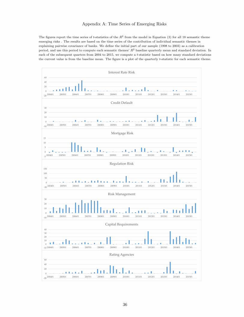
Appendix A: Time Series of Emerging Risks
The figures report the time series of t-statistics of the R2 from the model in Equation (3) for all 18 semantic theme
emerging risks . The results are based on the time series of the contribution of individual semantic themes in
explaining pairwise covariance of banks. We define the initial part of our sample (1998 to 2003) as a calibration
period, and use this period to compute each semantic themes’ R2 baseline quarterly mean and standard deviation. In
each of the subsequent quarters from 2004 to 2015, we compute a t-statistic based on how many standard deviations
the current value is from the baseline mean. The figure is a plot of the quarterly t-statistic for each semantic theme.
‐20
0
20
40
60
200401 200501 200601 200701 200801 200901 201001 201101 201201 201301 201401 201501
Interest Rate Risk
‐10
0
10
20
30
200401 200501 200601 200701 200801 200901 201001 201101 201201 201301 201401 201501
Credit Default
‐5
0
5
10
15
200401 200501 200601 200701 200801 200901 201001 201101 201201 201301 201401 201501
Mortgage Risk
‐50
0
50
100
150
200401 200501 200601 200701 200801 200901 201001 201101 201201 201301 201401 201501
Regulation Risk
‐10
0
10
20
30
200401 200501 200601 200701 200801 200901 201001 201101 201201 201301 201401 201501
Risk Management
‐10
0
10
20
30
40
200401 200501 200601 200701 200801 200901 201001 201101 201201 201301 201401 201501
Capital Requirements
‐20
0
20
40
60
200401 200501 200601 200701 200801 200901 201001 201101 201201 201301 201401 201501
Rating Agencies
36

Appendix A: Time Series of Emerging Risks (continued)
fv
‐20
0
20
40
200401 200501 200601 200701 200801 200901 201001 201101 201201 201301 201401 201501
Marketable Securities
‐5
0
5
10
200401 200501 200601 200701 200801 200901 201001 201101 201201 201301 201401 201501
Fair Value
‐20
0
20
40
200401 200501 200601 200701 200801 200901 201001 201101 201201 201301 201401 201501
Taxes
‐5
0
5
10
200401 200501 200601 200701 200801 200901 201001 201101 201201 201301 201401 201501
Deposits
‐20
0
20
40
200401 200501 200601 200701 200801 200901 201001 201101 201201 201301 201401 201501
Funding Sources
‐5
0
5
10
15
200401 200501 200601 200701 200801 200901 201001 201101 201201 201301 201401 201501
Executive Compensation
‐50
0
50
100
200401 200501 200601 200701 200801 200901 201001 201101 201201 201301 201401 201501
Dividends
37

Appendix A: Time Series of Emerging Risks (continued)
-50
0
50
100
150
200401 200501 200601 200701 200801 200901 201001 201101 201201 201301 201401 201501
Real Estate
-10
0
10
20
200401 200501 200601 200701 200801 200901 201001 201101 201201 201301 201401 201501
Accounting
-10
0
10
20
200401 200501 200601 200701 200801 200901 201001 201101 201201 201301 201401 201501
Competition
-5
0
5
10
200401 200501 200601 200701 200801 200901 201001 201101 201201 201301 201401 201501
Derivative and Counterparty Risk
38

References
Acharya, Viral, Lasse Heje Pedersen, Thomas Philippon, and Matthew Richardson, 2012, Measuring sys-
temic risk, CEPR Discussion Paper.
Acharya, Viral V., Irvind Gujral, Nirupama Kulkarni, and Hyun Song Shin, 2011, Dividends and bank
capital in the financial crisis of 2007-2009, .
Adrian, Tobias, and Markus Brunnermeier, 2016, Co va r, American Economic Review forthcoming.
Aebia, Vincent, Gabriele Sabatob, and Markus Schmid, 2012, Risk management, corporate governance, and
bank performance in the financial crisis, Journal of Banking and Finance 26, 32133226.
Allen, Franklin, Ana Babus, and Elena Carletti, 2012, Asset commonality, debt maturity and systemic risk,
Journal of Financial Economics 104, 519 – 534.
Alvarez, Fernando, and Gadi Barlevy, 2015, Mandatory disclosure and financial contagion, .
Andolfatto, David, Aleksander Berentsen, and Christopher Waller, 2014, Optimal disclosure policy and
undue diligence, Journal of Economic Theory 149, 128–152.
Ball, Christopher, Gerard Hoberg, and Vojislav Maksimovic, 2016, Disclosure, business change, and earnings
quality, University of Maryland and University of Southern California Working Paper.
Barber, Brad M., and Terrance Odean, 2007, All that glitters: The effect of attention and news on the
buying behavior of individual and institutional investors, Review of Financial Studies 21, 785–818.
Becker, Bo, and Todd Milbourn, 2011, How did increased competition affect credit ratings?, Journal of
Financial Economics 101, 493–514.
Begley, Taylor, Amiyatosh Purnanandam, and Kuncheng (K.C.) Zheng, 2016, The strategic under-reporting
of bank risk, .
Bekaert, Geert, and Marie Hoerova, 2014, The vix, the variance premium and stock market volatility, Journal
of Econometrics 183, 181–192.
Benmelech, Efraim, and Jennifer Dlugosz, 2009, The alchemy of cdo credit ratings, Journal of Monetary
Economics 56, 617–634.
Berger, Allen, and Christa Bouwman, 2009, Bank liquidity creation, RFS 22, 3779–3837.
Berger, Allen, and Christa Bouwman, 2013, How does capital affect bank performance during financial
crises?, JFE 109, 146–176.
Beyer, Anne, Daniel A. Cohen, Thomas Z. Lys, and Beverly R. Walther, 2010, The financialreportingenvi-
ronment:reviewoftherecentliterature, Journal of Accounting and Economics 50, 296–343.
Billio, Monica, Mila Getmansky, Andrew W. Lo, and Loriana Pelizzon, 2012, Econometric measures of
connectedness and systemic risk in the finance and insurance sectors, Journal of Financial Economics
104, 535 – 559.
Bisias, Dimitrios, Mark Flood, Andrew W. Lo, and Stavros Valavanis, 2012, A survey of systemic risk
analytics, Annual Review of Financial Economics 4, 255–296.
Blei, David, A Ng, and M Jordan, 2003, Latent dirichlet allocation, Journal of Machine Learning Research
3, 993–1002.
Bolton, Patrick, Xavier Freixas, and Joel Shapiro, 2012, The credit ratings game, The Journal of Finance
67, 85–111.
Bouvard, Matthieu, Pierre Chaigneau, and Adolfo De Motta, 2016, Transparency in the financial system:
Rollover risk and crises, Journal of Finance 70, 1805–1837.
Brunnermeier, Markus, Gary Gorton, and Arvind Krishnamurthy, 2014, Risk Topography . chap. Liquidity
Mismatch Measurement (University of Chicago Press).
Brunnermeier, Markus K., and Martin Oehmke, 2013, Bubbles, Financial Crises, and Systemic Risk (Hand-
book of the Economics of Finance).
Bui, Dien, Chih-Yung Lin, and Tse-Chun Lin, 2016, Yesterday once more: Short selling and two banking
crises, University of Hong Kong Working Paper.
39

Bussiere, Matthieu, and Marcel Fratzscher, 2006, Towards a new early warning system of financial crises,
Journal of International Money and Finance 25, 953–973.
Cole, Rebel, and Lawrence White, 2011, Deja vu all over again: The causes of u.s. commercial bank failures
this time around, Journal of Financial Services Research 42, 5–29.
Cornett, Marcia Millon, Jamie John McNutt, Philip E. Strahan, and Hassan Tehranian, 2011, Liquidity risk
management and credit supply in the financial crisis, Journal of Financial Economics 101, 297–312.
Covitz, Daniel, Nellie Liang, and Gustavo Suarez, 2013, The evolution of a financial crisis: Collapse of the
asset-backed commercial paper market, Journal of Finance 68, 815–848.
Dang, Tri Vi, Gary Gorton, Bengt Holstrom, and Guillermo Ordonez, 2016, Banks as secret keepers, Yale
University Working Paper.
Demyanyk, Yuliya, and Otto Van Hemert, 2011, Understanding the subprime mortgage crisis, RFS 24,
1848–1880.
DeYoung, Robert, and Gokhan Torna, 2013, Nontraditional Banking Activities and Bank Failures During
the Financial Crisis . , vol. 22 (Journal of Financial Intermediation).
Diamond, Douglas, and Phillip Dybvig, 1983, Bank runs, deposit insurance, and liquidity, Journal of Political
Economy 91, 401–419.
Diamond, Douglas, and Robert Verrecchia, 1987, Constraints on short-selling and asset price adjustment to
new information, JFE 18, 277–311.
Duca, Marco Lo, and Tuomas A. Peltonen, 2013, Assessing systemic risks and predicting systemic events,
Journal of Banking & Finance 37, 2183–2195.
Dwyer, Gerald P., and Paula Tkac, 2009, The financial crisis of 2008 in fixed-income markets, Journal of
International Money and Finance 28, 1293–1316.
Dye, Ronald A., 2001, An evaluation of ”essays on disclosure” and the disclosure literature in accounting,
Journal of Accounting and Economics 32, 181–235.
Elliot, Matthew, Benjamin Golub, and Matthew Jackson, 2014, Financial networks and contagion, American
Economic Review 104, 3115–3153.
Estrella, Arturo, and Frederic Mishkin, 2016, Predicting u.s. recessions: Financial variables as leading
indicators, The Review of Economics and Statistics pp. 45–61.
Fahlenbrach, Rudiger, Robert Prilmeier, and Rene Stulz, 2012, This time is the same: Using bank per-
formance in 1998 to explain bank performance during the recent financial crisis, Journal of Finance 67,
2139–2185.
Fahlenbrach, Rudiger, and Rene M. Stulz, 2011, Bank ceo incentives and the credit crisis, Journal of Finan-
cial Economics 99, 11–26.
Fama, Eugene, and Kenneth French, 1993, Common risk factors in stock and bond returns, Journal of
Financial Economics 33, 3–56.
Fama, Eugene, and J. MacBeth, 1973, Risk, return and equilibrium: Empirical tests, Journal of Political
Economy 71, 607–636.
Firth, John Rupert, 1957, A synopsis of linguistic theory 1930-55 (Frank Palmer) published 1968.
Flannery, Mark J., Simon H. Kwan, and Mahendrarajah Nimalendran, 2013, The 20072009 financial crisis
and bank opaqueness, Journal of Financial Intermediation 22, 55–84.
Frankel, Jeffrey, and George Saravelos, 2012, Can leading indicators assess country vulnerability? evidence
from the 2008-09 global financial crisis, Journal of International Economics 87, 216–231.
Frankel, Richard, Jared Jennings, and Joshua Lee, 2016, Using unstructured and qualitative disclosures to
explain accruals, Journal of Accounting and Economics forthcoming.
Gao, Lee, 2016, Text-implied risk and the cross-section of expected stock returns, .
Giesecke, Kay, and Baeho Kim, 2011, Systemic risk: What defaults are telling us, Management Science 57,
1387–1405.
Goel, Anand M., and Anjan V. Thakor, 2015, Information reliability and welfare: a theory of coarse credit
ratings, Journal of Financial Economics 115, 541–557.
40
Gorton, Gary, and Guillermo Ordonez, 2014, Collateral crises, American Economic Review 104, 343–378.
Gorton, Gary, and George Pennacchi, 1990, Financial intermediaries and liquidity creation, Journal of
Finance 45, 49–71.
Griffin, John M., Jordan Nickerson, and Dragon Yongjun Tang, 2013, Rating shopping or catering?an
examination of the response to competitive pressure for cdo credit ratings, Review of Financial Studies
26, 2270–2310.
Griffin, John M., and Dragon Yongjun Tang, 2012, Did subjectivity play a role in cdo credit ratings?, The
Journal of Finance 67, 1293–1328.
Hanley, Kathleen, and Gerard Hoberg, 2010, The information content of IPO prospectuses, Review of Fi-
nancial Studies 23, 2821–2864.
Hanley, Kathleen, and Gerard Hoberg, 2012, Litigation risk and the underpricing of initial public offerings,
Journal of Financial Economics 103, 235–254.
He, Jie, Jun Qian, and Philip Strahan, 2011, Credit ratings and the evolution of the mortgage-backed
securities market, American Economic Review 101, 131–135.
Healy, Paul, and Krishna Palepu, 2001, nformation asymmetry, corporate disclosure, and the capital markets:
A review of the empirical disclosure literature, Journal of Accounting and Economics 31, 405–440.
Hoberg, Gerard, 2016, Discussion of using unstructured and qualitative disclosures to explain accruals,
Forthcoming Discussion in the Journal of Accounting and Economics.
Hoberg, Gerard, and Vojislav Maksimovic, 2015, Redefining financial constraints: a text-based analysis,
Review of Financial Studies 28, 1312–1352.
Hoberg, Gerard, and Gordon Phillips, 2010, Product market synergies in mergers and acquisitions: A text
based analysis, Review of Financial Studies 23, 3773–3811.
Hoberg, Gerard, and Gordon Phillips, 2016, Text-based network industry classifications and endogenous
product differentiation, Journal of Political Economy.
Huang, Xin, Hao Zhou, and Haibin Zhu, 2009, A framework for assessing the systemic risk of major financial
institutions, Journal of Banking and Finance 33, 2036–2049.
Jeffrey S. Jones, and Wayne Y. Lee, and Timothy J. Yeager, 2013, Valuation and systemic risk consequences
of bank opacity, Journal of Financial Information 37, 693–706.
Kurlat, Pablo, and Laura Veldkamp, 2015, Should we regulate financial information?, Journal of Economic
Theory 158, 697–720.
Loughran, Tim, and Bill McDonald, 2011, When is a liability not a liability? Textual analysis, dictionaries,
and 10-Ks, Journal of Finance 66, 35–65.
Loughran, Tim, and Bill McDonald, 2014, Measuring readability in financial text, JF 69, 1643–1671.
Manela, Asaf, and Alan Moreira, 2016, News implied volatility and disasters concerns, Journal of Financial
Economics forthcoming.
Merton, Robert, 1986, A simple model of capital market equilibrium with incomplete information, JF 42,
482–510.
Mian, Atif, and Amir Sufi, 2009, The consequences of mortgage credit expansion: Evidence from the u.s.
mortgage default crisis, The Quarterly Journal of Economics 124, 1449–1496.
Mikolov, T., K. Chen, G. Corrado, and J. Dean, 2013, Efficient estimation of word representations in vector
space, CoRR abs/1301.3781.
Mikolov, T., I. Sutskever, K. Chen, G. Corrado, and J. Dean, 2013, Distributed representations of words and
phrases and their compositionality, Advances in neural information processing systems pp. 3111–3119.
Morgan, Donald P., 2002, Rating banks: Risk and uncertainty in an opaque industry, American Economic
Review 92, 874–888.
Peristian, Stavros, Donald P. Morgan, and Vanessa Savino, 2010, The information value of the stress test
and bank opacity, .
Sarkar, Sumit, and Ram S. Sriram, 2001, Bayesian models for early warning of bank failures., Management
Science 47, 1457–1475.
41

Shleifer, Andrei, and Robert Vishny, 1997, The limits of arbitrage, Journal of Finance 52, 35–55.
Skreta, Vasiliki, and Laura Veldkamp, 2009, Ratings shopping and asset complexity: A theory of ratings
inflation, Journal of Monetary Economics 56, 678–695.
Stulz, Rene, 2010, Credit default swaps and the credit crisis, Journal of Economic Perspectives 24, 79–92.
Tetlock, Paul, 2010, Does public financial news resolve asymmetric information, Review of Financial Studies
23, 3520–3557.
Tetlock, Paul, Maytal Saar-Tsechanksy, and Sofus Macskassy, 2008, More than words: Quantifying language
to measure firms’ fundamentals, Journal of Finance 63, 1437–1467.
Tetlock, Paul C., 2007, Giving content to investor sentiment: The role of media in the stock market, Journal
of Finance 62, 1139–1168.
Verrecchia, Robert E., 2001, Essays on disclosure, Journal of Accounting and Economics 32, 97–180.
White, Lawrence J., 2010, Markets: The credit rating agencies, Journal of Economic Perspectives 24, 211–
226.
42

Fig
ure
1:A
ggre
gate
Syst
emic
Ris
kM
easu
re
Aggre
gate
mea
sure
of
syst
emic
risk
from
ou
rd
yn
am
icem
ergin
gri
sks
mod
el.
Th
em
easu
reis
the
(norm
alize
d)
ad
just
edR
2co
ntr
ibu
tion
top
air
wis
ere
turn
covari
an
ceof
ban
kst
ock
sof
all
of
the
18
sem
anti
cth
emes
extr
act
edfr
om
10-K
dis
close
db
an
kri
skfa
ctors
from
1998
to2015.
‐202468101214
199801
199901
200001
200101
200201
200301
200401
200501
200601
200701
200801
200901
201001
201101
201201
201301
201401
201501
43

Figure 2: Emerging Risks Using LDA with 25 Topics
Overview of the 25 risk factors detected by metaHeuristica from the corpus of bank risk factors disclosed in fiscal
years ending in 2006.
44
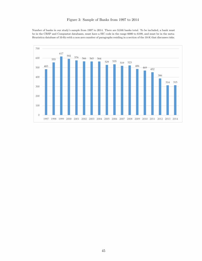
Figure 3: Sample of Banks from 1997 to 2014
Number of banks in our study’s sample from 1997 to 2014. There are 9,046 banks total. To be included, a bank must
be in the CRSP and Compustat databases, must have a SIC code in the range 6000 to 6199, and must be in the meta-
Heuristica database of 10-Ks with a non-zero number of paragraphs residing in a section of the 10-K that discusses risks.
483
555
617592 576 566 565 564
529 535 519 523486 469 452
386
314 315
0
100
200
300
400
500
600
700
1997 1998 1999 2000 2001 2002 2003 2004 2005 2006 2007 2008 2009 2010 2011 2012 2013 2014
45

Figure 4: Emerging Risks Comparison
Time series of t-statistics for semantic theme emerging risk variables. We define the initial part of our sample (1998
to 2003) as a calibration period, and use this period to compute each variable’s baseline quarterly mean and standard
deviation. In each of the subsequent quarters from 2004 to 2015, we compute a t-statistic based on how many
standard deviations the current value is from the baseline mean. The figure is a plot of each variable’s quarterly
t-statistics. Panel A displays the time series of t-statistics for the VIX index, and the quarterly average pairwise
covariance among bank-pairs. We also report t-statistics for the average quarterly standard deviation of monthly
returns across all stocks in the CRSP database and for financial firms only (SIC codes from 6000 to 6199). Panel B
reports t-statistics for the R2 of the accounting and text variables created by our covariance emerging risk model.
Panel A: Financial Market Variables
Panel B: Accounting and Textual Semantic Themes
‐10
0
10
200401 200501 200601 200701 200801 200901 201001 201101 201201 201301 201401 201501
VIX Level
‐10
0
10
200401 200501 200601 200701 200801 200901 201001 201101 201201 201301 201401 201501
Accounting Variables
0
10
20
200401 200501 200601 200701 200801 200901 201001 201101 201201 201301 201401 201501
Semantic Themes
‐50
0
50
100
200401 200501 200601 200701 200801 200901 201001 201101 201201 201301 201401 201501
Average Covariance
‐5
0
5
200401 200501 200601 200701 200801 200901 201001 201101 201201 201301 201401 201501
Std Dev Returns (All)
‐5
0
5
200401 200501 200601 200701 200801 200901 201001 201101 201201 201301 201401 201501
Std Dev Returns (Financials)
‐15
5
25
200401 200501 200601 200701 200801 200901 201001 201101 201201 201301 201401 201501
LDA Topics
46

Figure 5: Crisis Period Emerging Risks
Time series of t-statistics of the R2 from the model in Equation (3) for the most prominent emerging risk
in 2008 (Appendix A presents all 18 semantic theme emerging risks). The results are based on the time
series of the contribution of individual semantic themes in explaining pairwise covariance of banks. We
define the initial part of our sample (1998 to 2003) as a calibration period, and use this period to com-
pute each semantic themes’ R2 baseline quarterly mean and standard deviation. In each of the subsequent
quarters from 2004 to 2015, we compute a t-statistic based on how many standard deviations the cur-
rent value is from the baseline mean. The figure is a plot of the quarterly t-statistic for each semantic theme.
-5
0
5
10
15
200401 200501 200601 200701 200801 200901 201001 201101 201201 201301 201401 201501
Mortgage Risk
-50
0
50
100
200401 200501 200601 200701 200801 200901 201001 201101 201201 201301 201401 201501
Real Estate
-20
0
20
40
200401 200501 200601 200701 200801 200901 201001 201101 201201 201301 201401 201501
Marketable Securities
0
20
40
60
200401 200501 200601 200701 200801 200901 201001 201101 201201 201301 201401 201501
Dividends
-20
0
20
40
60
200401 200501 200601 200701 200801 200901 201001 201101 201201 201301 201401 201501
Interest Rate Risk
-20
0
20
40
200401 200501 200601 200701 200801 200901 201001 201101 201201 201301 201401 201501
Rating Agencies
-10
40
90
200401 200501 200601 200701 200801 200901 201001 201101 201201 201301 201401 201501
Regulation Risk
-10
0
10
20
30
200401 200501 200601 200701 200801 200901 201001 201101 201201 201301 201401 201501
Risk Management
47

Figure 6: Current Period Emerging Risks
Time series of t-statistics of the R2 from the model in Equation (3) for the most prominent emerging risk
in 2015 (Appendix A presents all 18 semantic theme emerging risks). The results are based on the time
series of the contribution of individual semantic themes in explaining pairwise covariance of banks. We
define the initial part of our sample (1998 to 2003) as a calibration period, and use this period to com-
pute each semantic themes’ R2 baseline quarterly mean and standard deviation. In each of the subsequent
quarters from 2004 to 2015, we compute a t-statistic based on how many standard deviations the cur-
rent value is from the baseline mean. The figure is a plot of the quarterly t-statistic for each semantic theme.
-20
0
20
40
200401 200501 200601 200701 200801 200901 201001 201101 201201 201301 201401 201501
Funding Sources
-5
0
5
10
200401 200501 200601 200701 200801 200901 201001 201101 201201 201301 201401 201501
Derivative and Counterparty Risk
-20
0
20
40
200401 200501 200601 200701 200801 200901 201001 201101 201201 201301 201401 201501
Marketable Securities
-10
10
30
200401 200501 200601 200701 200801 200901 201001 201101 201201 201301 201401 201501
Credit Default
-50
0
50
100
150
200401 200501 200601 200701 200801 200901 201001 201101 201201 201301 201401 201501
Regulation Risk
-10
0
10
20
30
200401 200501 200601 200701 200801 200901 201001 201101 201201 201301 201401 201501
Risk Management
-100
10203040
200401 200501 200601 200701 200801 200901 201001 201101 201201 201301 201401 201501
Capital Requirements
-50
0
50
100
150
200401 200501 200601 200701 200801 200901 201001 201101 201201 201301 201401 201501
Real Estate
48

Figure 7: Sub-Theme Emerging Risks
Time series of t-statistics for sub-themes related to the semantic theme “Marketable Securities.” We de-
fine the initial part of our sample (1998 to 2003) as a calibration period, and use this period to compute
each semantic sub-themes’ R2 baseline quarterly mean and standard deviation. In each of the subsequent
quarters from 2004 to 2015, we compute a t-statistic based on how many standard deviations the cur-
rent value is from the baseline mean. The figure is a plot of the quarterly t-statistic for each semantic theme.
-10
0
10
20
30
200401 200501 200601 200701 200801 200901 201001 201101 201201 201301 201401 201501
Mortgage-Backed Securities
-10
0
10
20
30
200401 200501 200601 200701 200801 200901 201001 201101 201201 201301 201401 201501
Commercial Paper
-40
10
60
200401 200501 200601 200701 200801 200901 201001 201101 201201 201301 201401 201501
Cash
-20
0
20
40
200401 200501 200601 200701 200801 200901 201001 201101 201201 201301 201401 201501
Municipal Bonds
49

Tab
leI:
Exam
ple
sof
Sem
anti
cV
ecto
rs
Foca
lw
ord
an
dp
hra
selist
sfo
rsi
xof
the
18
sem
anti
cth
emes
der
ived
from
Late
nt
Dir
ich
let
Alloca
tion
on
the
risk
fact
or
dis
cuss
ion
of
pu
bli
cly
trad
edb
an
ks
(th
ose
havin
gS
ICco
des
inth
era
nge
6000
to6199).
Th
eti
tle
of
each
them
eis
the
short
on
eto
two
word
ph
rase
note
din
the
colu
mn
hea
der
s.F
or
each
of
the
six
them
es,
we
incl
ud
etw
oco
lum
ns.
Th
efi
rst
isth
elist
of
spec
ific
word
sor
ph
rase
sid
enti
fied
by
the
Sem
anti
cV
ecto
rm
od
ule
inm
etaH
euri
stic
aas
bei
ng
hig
hly
sim
ilar
toth
eth
eme’
sti
tle.
Th
ese
con
dis
each
word
’sco
sin
esi
milari
tyto
the
them
e’s
titl
e.
Mort
gage
Ris
kC
ap
ital
Req
uir
emen
tsD
eriv
ati
ve
&C
ou
nte
rpart
yR
isk
Fair
Valu
eD
eposi
tR
isk
Com
pet
itio
n
Cosi
ne
Cosi
ne
Cosi
ne
Cosi
ne
Cosi
ne
Cosi
ne
Row
Word
Dis
tW
ord
Dis
tW
ord
Dis
tW
ord
Dis
tW
ord
Dis
tW
ord
Dis
t
1m
ort
gages
1ca
pit
al
0.7
89
cou
nte
rpart
y1
fair
0.9
61
dep
osi
ts1
com
pet
itio
n1
2m
ort
gage
0.7
974
requ
irem
ents
0.7
89
cou
nte
rpart
ies
0.8
916
valu
e0.9
61
dep
osi
t0.8
211
com
pet
e0.7
932
3im
pac
alt
0.7
148
mee
t0.5
369
cou
nte
rpart
y’s
0.8
009
valu
es0.6
277
bro
ker
edd
e-p
osi
ts0.7
59
inte
nse
com
pe-
titi
on
0.7
822
4re
sid
enti
al
mort
gage
0.7
085
regu
lato
ry0.4
508
net
tin
g0.7
556
valu
ati
on
tech
-n
iqu
es0.5
068
bro
ker
edce
rtifi
-ca
tes
0.7
406
hig
hly
com
pet
i-ti
ve
0.7
798
5ori
gin
ate
d0.6
939
ad
dit
ion
al
0.4
422
cou
nte
rpart
yn
on
per
form
an
0.6
873
esti
mate
d0.4
865
non
inte
rest
bea
ring
0.7
382
com
pet
ing
0.7
504
6re
sid
enti
al
mort
gages
0.6
922
cap
ital
exp
en-
dit
ure
0.4
404
non
per
form
an
ce0.6
869
valu
ati
on
met
hod
olo
gie
s0.4
857
bea
rin
gch
eck-
ing
0.7
213
extr
emel
yco
m-
pet
itiv
e0.7
454
7ad
just
ab
lera
te0.6
726
min
imu
m0.4
278
mast
ern
etti
ng
0.6
704
valu
ati
on
0.4
823
bea
rin
gd
e-p
osi
ts0.7
175
com
pet
es0.7
327
8co
llate
ralizi
ng
0.6
372
exp
end
itu
res
0.4
273
anti
cip
ate
non
-p
erfo
rman
ce0.6
604
carr
yin
g0.4
749
pass
book
0.6
71
com
pet
itors
0.7
297
9ori
gin
ati
on
s0.6
363
requ
irem
ent
0.4
228
net
tin
gar-
ran
gem
ents
0.6
278
dis
cou
nte
d0.4
666
chec
kin
gac-
cou
nts
0.6
655
face
inte
nse
0.7
266
10
fhlm
c0.6
303
iub
fsb
0.4
166
pare
nta
lgu
ar-
ante
es0.5
735
qu
ote
d0.4
645
cdars
0.6
372
face
sco
mp
eti-
tion
0.7
141
11
fnm
a0.6
271
fun
d0.4
096
swap
0.5
659
asc
820
0.4
569
jum
bo
cert
ifi-
cate
s0.6
316
face
com
pet
i-ti
on
0.7
138
12
fan
nie
mae
0.6
231
liqu
idit
y0.4
07
collate
ral
post
-in
gs
0.5
643
valu
ati
on
tech
-n
iqu
e0.4
551
bro
ker
ed0.6
274
com
pet
itiv
e0.7
123
13
sin
gle
fam
ily
0.6
174
com
ply
0.4
004
cou
nte
rpart
yow
es0.5
615
natu
rald
rive
conti
ngen
t0.4
507
pass
book
sav-
ings
0.6
181
inte
nse
0.7
117
14
fred
die
mac
0.6
156
rati
os
0.3
963
isd
a0.5
571
mea
suri
ng
0.4
485
mm
da
0.6
11
inte
nsi
fy0.6
999
15
mb
s0.6
142
regu
lati
on
s0.3
939
swap
s0.5
568
un
der
lyin
g0.4
403
swee
pacc
ou
nts
0.5
862
com
pet
eeff
ec-
tivel
y0.6
993
16
ori
gin
ate
0.6
095
sati
sfy
0.3
9cr
edit
wort
hy
cou
nte
rpart
i0.5
529
pri
cin
gm
od
els
0.4
349
cdars
pro
gra
m0.5
836
entr
ants
0.6
973
17
new
lyori
gi-
nate
d0.6
069
requ
ired
0.3
864
ass
oci
ati
on
isd
a0.5
517
valu
ing
0.4
334
borr
ow
edfu
nd
s0.5
818
face
sin
ten
se0.6
799
18
ass
oci
ati
on
fnm
a0.6
06
gu
idel
ines
0.3
836
isd
am
ast
er0.5
46
115
aacc
ou
nt-
ing
0.4
27
chec
kin
gsa
v-
ings
0.5
724
inte
nse
lyco
m-
pet
itiv
e0.6
721
19
mort
gage
back
ed0.6
052
regu
lato
rs0.3
798
exp
osu
re0.5
252
mea
sure
d0.4
223
bro
ker
edcd
s0.5
678
com
pet
esu
c-ce
ssfu
lly
0.6
644
20
loan
ori
gin
a-
tion
s0.6
049
nee
ds
0.3
781
marg
inin
g0.5
242
det
erm
ined
0.4
217
cdars
dep
osi
ts0.5
526
low
barr
iers
0.6
563
50

Tab
leII
:P
ears
onC
orre
lati
onC
oeffi
cien
ts(S
eman
tic
Th
emes
)
Pea
rson
corr
elati
on
coeffi
cien
tsfo
rth
e18
sem
anti
cth
emes
der
ived
from
Late
nt
Dir
ich
let
All
oca
tion
on
the
risk
fact
or
dis
cuss
ion
of
pu
blicl
ytr
ad
edb
an
ks
(th
ose
havin
gS
ICco
des
inth
era
nge
6000
to6199).
Inte
rest
Mort-
Fund-
Rate
Cre
dit
gage
Regul.
Risk
Capital
Rating
Mkt
Fair
Depo-
ing
Exec.
Div-
Real
Acc-
Comp-
Variable
Risk
Default
Risk
Risk
Mgmt
Req.
Agen.
Secur.
Valu
eTaxes
sits
Sourc
es
Comp.
idends
Estate
ounting
etition
Cre
dit
Default
-0.287
MortgageRisk
0.005
0.237
Regulation
Risk
-0.274
0.061
0.139
Risk
Management
0.268
0.174
0.006
0.025
CapitalReq.
-0.265
0.173
0.090
0.667
0.131
Rating
Agencies
-0.101
0.149
0.070
0.143
0.177
0.196
Mark
eta
ble
Sec.
0.134
0.009
0.220
0.124
0.233
0.388
0.110
Fair
Valu
e0.332
0.017
0.166
-0.063
0.268
0.125
0.006
0.547
Taxes
0.395
-0.125
0.113
0.071
0.147
0.179
0.027
0.452
0.522
Deposits
0.172
0.016
0.179
0.352
0.108
0.375
-0.002
0.355
0.239
0.281
Fundin
gSourc
es
-0.006
0.220
0.139
0.392
0.286
0.632
0.199
0.394
0.091
0.142
0.384
ExecutiveComp.
-0.025
-0.003
0.115
0.202
0.177
0.303
0.075
0.353
0.392
0.397
0.220
0.166
Divid
ends
-0.186
0.010
0.074
0.520
0.015
0.693
0.068
0.392
0.263
0.310
0.343
0.389
0.456
RealEstate
-0.232
0.315
0.430
0.331
-0.051
0.233
0.025
0.029
-0.040
-0.010
0.203
0.162
0.065
0.210
Accounting
-0.151
0.114
0.085
0.166
0.191
0.329
0.049
0.443
0.575
0.420
0.174
0.159
0.475
0.406
0.019
Competition
-0.206
0.084
0.086
0.674
0.037
0.423
0.078
-0.003
-0.152
-0.045
0.273
0.369
0.098
0.378
0.321
0.035
Deriv+Counte
rparty
0.236
0.269
-0.042
-0.275
0.491
-0.118
0.110
0.064
0.254
-0.038
-0.192
0.006
-0.066
-0.188
-0.188
0.084
-0.245
51

Table III: Summary Statistics
Summary statistics for our sample of 9,046 bank-year observations from 1998 to December 2015. Panel A reports sum-mary statistics based on bank-pair-quarter observations (55.4 million observations). The bank-pair daily covarianceis the quarterly covariance of daily stock returns for a pair of banks. Bank-pair SIC variables are dummy variablesequal to one if the pair of banks is in the same 2, 3 or 4 digit SIC-based industry, zero otherwise. The TNIC similarityfor a pair of banks is from Hoberg and Phillips (2010). The bank-level variables in Panel B is based on Compustatdata and includes Ln(Assets) and Ln(Bank Age), the time since the first appearance in CRSP. Panel C is based onCall Reports and includes it Cash/Assets, Loans/Assets, Loan Loss Prov & Allow, the sum of loan loss provisionand allowances, Capital, the ratio of equity to assets, Neg. Earnings Dummy an indicator variable equal to one ifnet income is negative, zero otherwise, Bank Holding Co. Dummy, an indicator variable equal to one if the bankhas a parent, zero otherwise, Non-Performing Assets, the sum of loans that are 30 days and 90 days past due, andCatFat/Assets from Berger and Bouwman (2009). Panel D reports statistics for key time series variables. There are72 quarterly observations in our database from 1998 to 2015. The average pair covariance is the quarterly averagepairwise covariance among bank-pairs. We also report the average quarterly standard deviation of monthly returnsacross all stocks in the CRSP database and for financial firms only (SIC codes from 6000 to 6199). The accountingvariable adjusted R2 is the quarterly adjusted R2 from a regression of bank-pairwise correlation on the bank char-acteristics and industry variables. The text variable adjusted R2 is the incremental improvement to R2 when verbalfactors are also included in the pairwise covariance regression. Daily covariance figures are multiplied by 10,000 forease of viewing.
Std.
Variable Mean Dev. Minimum Median Maximum # Obs.
Panel A: Bank-pair level data
Bank-Pair Daily Covariance 0.913 3.557 -225.51 0.373 329.975 55,412,642
Bank-Pair Same 2-digit SIC 0.872 0.333 0.000 1.000 1.000 55,412,642
Bank-Pair Same 3-digit SIC 0.499 0.499 0.000 0.484 1.000 55,412,642
Bank-Pair Same 4-digit SIC 0.468 0.498 0.000 0.178 1.000 55,412,642
Bank-Pair TNIC Similarity 0.090 0.077 0.000 0.088 0.755 55,412,642
Panel B: Bank-level data (Compustat)
Ln(Assets) 7.308 1.616 1.584 7.007 14.598 9,046
Ln(Bank Age) 2.118 0.897 0.000 2.303 3.970 9,046
Panel C: Bank-level data (Call Reports)
Cash/Assets 0.042 0.035 0.000 0.033 0.336 7,169
Loans/Assets 0.496 0.178 0.000 0.503 0.907 7,169
Loss Prov & Allow/Assets 0.002 0.004 -0.004 0.001 0.057 7,169
Capital 0.100 0.041 0.008 0.093 1.000 7,169
Negative Earnings Dummy 0.050 0.218 0.000 0.000 1.000 7,168
Bank Holding Co. Dummy 0.850 0.357 0.000 1.000 1.000 7,169
Non-Performing Assets/Assets 0.005 0.007 0.000 0.003 0.056 7,169
CatFat/Assets 6.908 366.698 -0.546 0.389 25965.9 7,169
Panel D: Time-series data
VIX Index 21.227 7.594 11.190 20.425 51.723 72
Avg Pair Covariance 1.074 2.069 0.150 0.437 12.704 72
Avg Std Dev Monthly Returns 0.155 0.050 0.095 0.134 0.307 72
Avg Std Dev Monthly Returns (FinancialsOnly)
0.091 0.032 0.050 0.083 0.171 72
Accounting Variable Adj R2 0.078 0.061 0.005 0.054 0.237 72
Text Variable Adj R2 0.009 0.007 0.000 0.008 0.025 72
52

Tab
leIV
:P
ears
onC
orre
lati
onC
oeffi
cien
ts(T
ime
Ser
ies
Vari
able
s)
Pea
rson
Corr
elati
on
Coeffi
cien
tsare
rep
ort
edfo
rou
rkey
tim
ese
ries
vari
ab
les.
Th
ere
are
72
qu
art
erly
ob
serv
ati
on
sin
ou
rd
ata
base
from
1998
to2015.
Th
eaver
age
pair
covari
an
ceis
the
qu
art
erly
aver
age
pair
wis
eco
vari
an
ceam
on
gb
an
k-p
air
s.W
eals
ore
port
the
aver
age
qu
art
erly
stan
dard
dev
iati
on
of
month
lyre
turn
sacr
oss
all
stock
sin
the
CR
SP
data
base
an
dfo
rfi
nan
cial
firm
son
ly(S
ICco
des
from
6000
to6199).
Th
eacc
ou
nti
ng
vari
ab
lead
just
edR
2is
the
qu
art
erly
ad
just
edR
2fr
om
are
gre
ssio
nof
ban
k-p
air
wis
eco
rrel
ati
on
on
the
ban
kch
ara
cter
isti
csan
din
du
stry
vari
ab
les.
Th
ete
xt
vari
ab
lead
just
edR
2is
the
incr
emen
tal
imp
rovem
ent
toR
2w
hen
ver
bal
fact
ors
are
als
oin
clu
ded
inth
ep
air
wis
eco
vari
an
cere
gre
ssio
n.
Acc
ou
nti
ng
Tex
tA
vg
Avg
Vari
ab
leV
ari
ab
leV
IXP
air
wis
eS
tdD
ev
Row
Vari
ab
leA
djR
2A
djR
2In
dex
Covari
an
ceR
etu
rns
(1)
Tex
tV
ari
ab
leA
djR
20.5
26
(2)
VIX
Ind
ex0.2
92
-0.3
59
(3)
Avg
Pair
Covari
an
ce0.5
04
0.1
01
0.7
28
(4)
Avg
Std
Dev
Month
lyR
etu
rns
-0.1
58
-0.6
05
0.5
56
0.1
94
(5)
Avg
Std
Dev
Month
lyR
etu
rns
(Fin
an
cials
On
ly)
-0.0
49
-0.5
78
0.7
80
0.4
88
0.8
80
53

Tab
leV
:B
asel
ine
Sem
anti
cT
hem
esan
dB
ank
Ch
arac
teri
stic
s
Det
erm
inants
of
the
18
sem
anti
cth
emes
usi
ng
OL
Sre
gre
ssio
nu
sin
gb
an
kch
ara
cter
isti
cs.
Th
ed
epen
den
tvari
ab
lein
Pan
elA
isa
ban
k’s
load
ing
on
the
giv
enth
eme,
an
dth
ein
dep
end
ent
vari
ab
les
incl
ud
eb
an
kch
ara
cter
isti
csLn(A
ssets)
Loa
ns/Assets,
Loa
nLoss
Prov,
the
sum
of
loan
loss
pro
vis
ion
an
dallow
an
ces,
Capital,
the
rati
oof
equ
ity
toass
ets,
Neg.Earn
ings
Dummy
an
ind
icato
rvari
ab
leeq
ual
toon
eif
net
inco
me
isn
egati
ve,
zero
oth
erw
ise,
Non-P
erform
ingAssets,
the
sum
of
loan
sth
at
are
30
days
an
d90
days
past
du
e,an
dCatFat/Assets
from
Ber
ger
an
dB
ouw
man
(2009).
Pan
elB
list
sfo
ur
ad
dit
ion
al
sub
-th
emes
rela
ted
tom
ark
etab
lese
curi
ties
.t-
stati
stic
sare
inp
are
nth
eses
.A
llR
HS
vari
ab
les,
an
dea
chd
epen
den
tvari
ab
le,
are
stan
dard
ized
toh
ave
un
itst
an
dard
dev
iati
on
pri
or
toru
nn
ing
the
regre
ssio
nto
ensu
rea
rela
tive
inte
rpre
tati
on
inte
rms
of
magn
itu
des
.
Log
Loan
s/L
oss
Pro
v/
Cap
-N
eg.
CatF
at/
NP
A/
Ad
j
Row
Sem
anti
cT
hem
eA
sset
sA
sset
sA
sset
sit
al
Earn
.A
sset
sA
sset
sR
2
PanelA:Base
lineSemanticM
odel
0U
nex
p.
Top
icC
onte
nt
0.0
37
(1.9
8)
-0.0
39
(-2.1
9)
0.0
02
(0.1
8)
0.0
19
(1.2
6)
-0.0
25
(-2.1
8)
-0.0
04
(-0.8
1)
-0.0
19
(-1.6
6)
0.1
56
1In
tere
stR
ate
Ris
k-0
.014
(-0.6
7)
0.0
30
(1.3
9)
-0.0
23
(-1.4
8)
0.0
26
(1.4
3)
-0.0
21
(-1.6
0)
-0.0
15
(-2.2
4)
-0.0
60
(-3.8
6)
0.1
99
2C
red
itD
efau
lt-0
.061
(-2.6
1)
-0.0
13
(-0.5
4)
0.0
27
(1.5
1)
-0.0
60
(-3.3
6)
-0.0
21
(-1.6
8)
0.0
15
(2.0
0)
0.0
38
(1.7
5)
0.0
23
3M
ort
gage
Ris
k0.0
03
(0.1
3)
0.1
15
(5.1
1)
-0.0
40
(-2.4
1)
0.0
43
(1.8
0)
0.0
26
(1.8
7)
-0.0
19
(-2.4
6)
-0.0
19
(-1.2
2)
0.0
72
4R
egu
lati
on
Ris
k0.0
13
(0.8
0)
-0.0
18
(-1.2
8)
0.0
02
(0.1
1)
-0.0
03
(-0.2
3)
0.0
26
(1.8
6)
0.0
08
(1.5
4)
0.0
29
(1.8
3)
0.4
20
5R
isk
Man
agem
ent
0.0
97
(4.1
7)
-0.0
69
(-3.0
7)
0.0
26
(1.4
0)
-0.0
45
(-2.2
6)
-0.0
23
(-1.6
0)
0.0
22
(3.1
6)
0.0
26
(1.6
2)
0.1
09
6C
ap
ital
Req
.0.0
62
(3.7
3)
-0.0
46
(-2.9
2)
0.0
41
(2.7
1)
0.0
05
(0.4
2)
0.0
19
(1.3
2)
0.0
08
(1.6
3)
0.0
32
(2.6
6)
0.4
46
7R
ati
ng
Agen
cies
0.0
43
(3.0
9)
-0.0
32
(-2.8
6)
0.0
24
(1.0
3)
0.0
04
(0.2
9)
-0.0
18
(-0.9
7)
-0.0
01
(-0.3
8)
0.0
05
(0.2
6)
0.1
49
8M
ark
etab
leS
ec.
0.1
02
(4.2
8)
-0.0
00
(-0.0
1)
-0.0
42
(-2.0
9)
0.0
18
(0.9
1)
0.0
70
(4.1
8)
-0.0
04
(-0.6
7)
0.0
50
(2.7
0)
0.1
29
9F
air
Valu
e-0
.124
(-7.3
9)
0.0
25
(1.5
0)
-0.0
03
(-0.2
4)
-0.0
08
(-0.5
4)
-0.0
25
(-2.1
1)
-0.0
02
(-0.4
9)
-0.0
16
(-1.1
6)
0.3
08
10
Taxes
-0.0
19
(-0.7
0)
0.0
07
(0.2
7)
-0.0
46
(-2.4
7)
0.0
31
(1.3
1)
0.0
24
(1.2
4)
-0.0
13
(-1.5
0)
-0.0
42
(-2.3
2)
0.0
29
11
Dep
osi
ts0.0
12
(0.6
6)
-0.0
00
(-0.0
1)
0.0
23
(1.3
7)
0.0
21
(1.5
2)
0.0
44
(3.5
0)
0.0
03
(0.5
5)
0.0
40
(2.6
0)
0.1
93
12
Fu
nd
ing
Sou
rces
0.0
29
(1.7
4)
-0.0
34
(-2.1
7)
0.0
34
(2.3
6)
0.0
46
(3.3
1)
-0.0
11
(-0.9
1)
-0.0
11
(-2.0
4)
0.0
22
(1.5
9)
0.2
10
13
Exec
uti
ve
Com
p.
0.1
10
(5.0
0)
-0.0
22
(-1.3
2)
-0.0
05
(-0.3
3)
0.0
25
(1.5
4)
0.0
24
(1.8
9)
-0.0
02
(-0.2
4)
0.0
17
(1.2
2)
0.1
77
14
Div
iden
ds
-0.0
16
(-0.8
9)
0.0
17
(0.9
0)
0.0
36
(1.8
7)
0.0
25
(1.3
8)
0.0
46
(2.5
3)
-0.0
06
(-1.0
9)
0.0
16
(0.9
1)
0.2
40
15
Rea
lE
state
-0.0
77
(-3.3
6)
0.0
71
(3.4
5)
0.0
21
(1.2
4)
0.0
39
(1.6
9)
-0.0
04
(-0.3
1)
-0.0
14
(-2.0
6)
-0.0
24
(-1.5
8)
0.0
85
16
Acc
ou
nti
ng
-0.0
25
(-1.2
1)
-0.0
22
(-1.0
7)
-0.0
29
(-1.7
3)
-0.0
49
(-2.6
1)
0.0
00
(0.0
0)
0.0
13
(2.2
2)
0.0
26
(1.6
4)
0.0
48
17
Com
pet
iton
-0.0
11
(-0.6
0)
-0.0
42
(-2.3
2)
0.0
03
(0.1
9)
0.0
10
(0.6
3)
-0.0
00
(-0.0
0)
-0.0
04
(-0.9
4)
-0.0
17
(-1.1
0)
0.2
15
18
Der
iv+
Cou
nte
rpart
y0.1
81
(8.7
7)
-0.0
03
(-0.1
9)
-0.0
15
(-1.0
7)
0.0
04
(0.3
2)
0.0
09
(0.7
3)
0.0
06
(0.8
1)
-0.0
14
(-1.2
9)
0.1
80
PanelB:M
ark
etable
Sec
urity
Sub-T
hemes
19
Mu
nic
ipal
Bon
ds
0.1
04
(5.6
4)
0.0
76
(3.6
8)
-0.0
96
(-6.9
6)
-0.0
02
(-0.1
1)
0.0
45
(4.6
6)
-0.0
01
(-0.1
7)
0.0
28
(2.8
3)
0.2
22
20
Mort
gage
Back
edS
ec.
0.0
29
(1.1
0)
0.0
98
(3.9
3)
-0.0
61
(-3.4
7)
0.0
44
(1.8
0)
0.0
36
(2.2
7)
-0.0
17
(-2.3
3)
-0.0
19
(-1.0
9)
0.0
39
21
Com
mer
cial
Pap
er-0
.005
(-0.4
6)
-0.0
48
(-3.9
5)
0.0
74
(5.5
6)
-0.0
04
(-0.3
9)
-0.0
18
(-1.9
4)
0.0
03
(0.8
2)
0.0
05
(0.5
4)
0.3
48
22
Cash
0.0
95
(5.6
2)
0.0
03
(0.1
5)
-0.0
20
(-1.2
4)
0.0
18
(1.0
7)
0.0
31
(2.2
6)
-0.0
09
(-1.5
3)
0.0
11
(0.9
5)
0.3
27
54

Tab
leV
I:C
risi
san
dC
urr
ent
Per
iod
Ret
urn
Reg
ress
ion
s
Cro
ss-s
ecti
on
al
regre
ssio
ns
pre
dic
tin
gin
div
idu
al
ban
kou
tcom
esd
uri
ng
an
daft
erth
efi
nan
cial
cris
isan
du
nd
ercu
rren
tec
on
om
icco
nd
itio
ns
.F
or
the
cris
isp
erio
din
Pan
elA
,th
ed
epen
den
tvari
ab
leis
the
ban
k’s
stock
retu
rnfr
om
Sep
tem
ber
2008
toD
ecem
ber
2012.
For
the
curr
ent
per
iod
inP
an
elB
,th
ed
epen
den
tvari
ab
leis
the
ban
k’s
stock
retu
rnfr
om
Dec
emb
erof
2015
toF
ebru
ary
2016.
Th
ein
dep
end
ent
vari
ab
leof
inte
rest
,EmergingRiskExposu
re,
isth
equ
art
erly
pre
dic
ted
covari
an
ceb
ase
don
Equ
ati
on
3.
We
note
that
all
regre
ssio
ns
use
ex-a
nte
data
an
dare
pre
dic
tive
wh
enn
ote
das
such
inth
ePredictive
Tim
ing
colu
mn
.W
ein
clu
de,
bu
td
on
ot
dis
pla
yin
ord
erto
con
serv
esp
ace
,co
ntr
ols
for
ban
kch
ara
cter
isti
cs,
mom
entu
m,
log
book
tom
ark
etan
dth
elo
gm
ark
etca
pit
ali
zati
on
inea
chre
gre
ssio
n.
We
als
oin
clu
de
ind
ust
ryfi
xed
effec
tsb
ase
don
fou
r-d
igit
SIC
cod
es.t-
stati
stic
sare
rep
ort
edin
pare
nth
eses
.
PanelA:CrisisPeriod
PanelB:CurrentPeriod
Emerg
ing
Risk
Pre
dictive
Emerg
ing
Risk
Pre
dictive
Row
Quarter
Exposu
reObs
Tim
ing
Quarter
Exposu
reObs
Tim
ing
(1)
2004
1Q
-1.493
(-1.16)
412
Pre
dictive
—2010
1Q
-0.861
(-7.67)
357
Pre
dictive
(2)
2004
2Q
-3.609
(-3.19)
393
Pre
dictive
—2010
2Q
-0.658
(-2.93)
338
Pre
dictive
(3)
2004
3Q
-2.848
(-1.26)
393
Pre
dictive
—2010
3Q
-0.760
(-3.96)
338
Pre
dictive
(4)
2004
4Q
-0.420
(-0.26)
393
Pre
dictive
—2010
4Q
-0.867
(-2.68)
338
Pre
dictive
(5)
2005
1Q
1.014
(0.50)
454
Pre
dictive
—2011
1Q
-1.592
(-2.24)
360
Pre
dictive
(6)
2005
2Q
0.653
(0.40)
444
Pre
dictive
—2011
2Q
-1.843
(-2.98)
353
Pre
dictive
(7)
2005
3Q
0.659
(0.44)
444
Pre
dictive
—2011
3Q
-1.729
(-2.50)
353
Pre
dictive
(8)
2005
4Q
1.291
(0.85)
444
Pre
dictive
—2011
4Q
-1.169
(-1.94)
352
Pre
dictive
(9)
2006
1Q
0.337
(0.47)
488
Pre
dictive
—2012
1Q
-0.566
(-1.51)
369
Pre
dictive
(10)
2006
2Q
-4.107
(-3.04)
462
Pre
dictive
—2012
2Q
-0.424
(-2.94)
360
Pre
dictive
(11)
2006
3Q
-4.809
(-3.54)
462
Pre
dictive
—2012
3Q
-0.559
(-3.81)
360
Pre
dictive
(12)
2006
4Q
-4.863
(-3.03)
462
Pre
dictive
—2012
4Q
-0.341
(-1.23)
360
Pre
dictive
(13)
2007
1Q
-7.441
(-3.56)
517
Pre
dictive
—2013
1Q
-0.603
(-2.88)
372
Pre
dictive
(14)
2007
2Q
-7.169
(-4.03)
508
Pre
dictive
—2013
2Q
-0.888
(-3.58)
337
Pre
dictive
(15)
2007
3Q
-8.040
(-4.51)
507
Pre
dictive
—2013
3Q
-0.704
(-2.78)
337
Pre
dictive
(16)
2007
4Q
-8.332
(-3.85)
507
Pre
dictive
—2013
4Q
-0.649
(-2.53)
337
Pre
dictive
(17)
2008
1Q
-6.780
(-1.83)
545
Pre
dictive
—2014
1Q
-0.950
(-3.11)
346
Pre
dictive
(18)
2008
2Q
-6.788
(-1.93)
512
Pre
dictive
—2014
2Q
-0.758
(-1.55)
294
Pre
dictive
(19)
2008
3Q
-8.761
(-3.38)
512
Non-P
redictive
—2014
3Q
-1.522
(-3.88)
294
Pre
dictive
(20)
2008
4Q
-7.503
(-3.60)
512
Non-P
redictive
—2014
4Q
-1.706
(-6.22)
294
Pre
dictive
(21)
2009
1Q
-8.710
(-7.13)
563
Non-P
redictive
—2015
1Q
-1.327
(-3.25)
297
Pre
dictive
(22)
2009
2Q
-9.591
(-7.92)
521
Non-P
redictive
—2015
2Q
-1.738
(-5.31)
295
Pre
dictive
(23)
2009
3Q
-7.084
(-4.81)
520
Non-P
redictive
—2015
3Q
-1.806
(-7.17)
295
Pre
dictive
(24)
2009
4Q
-5.767
(-2.96)
519
Non-P
redictive
—2015
4Q
-1.373
(-3.25)
295
Non-P
redictive
55

Tab
leV
II:
Ban
kF
ailu
reR
egre
ssio
ns
Cro
ss-s
ecti
on
al
regre
ssio
ns
pre
dic
tin
gw
hic
hb
an
ks
fail
du
rin
gth
ep
erio
daft
erth
eL
ehm
an
ban
kru
ptc
yin
late
2008.
Th
ed
epen
den
tvari
ab
leis
ad
um
my
vari
ab
leeq
ual
toon
eif
ab
an
kw
as
ass
iste
dor
failed
du
rin
gth
ecr
isis
per
iod
,ze
rooth
erw
ise
as
ind
icate
don
the
FD
ICw
ebsi
te.
Th
issa
mp
leof
failed
ban
ks
incl
ud
eson
lyp
ub
licl
ytr
ad
edb
an
ks,
wit
hth
efi
rst
failu
res
occ
urr
ing
inN
ovem
ber
of
2008,
an
dth
ela
stin
Ju
ne
of
2012.
Th
ere
are
41
such
failu
res,
wit
h{2
,12,1
9,6
,2}
occ
urr
ing
inth
eyea
rs{2
008,2
009,2
010,2
011,2
012},
resp
ecti
vel
y.T
he
ind
epen
den
tvari
ab
leof
inte
rest
,EmergingRiskExposu
re,is
the
qu
art
erly
pre
dic
ted
covari
an
cebase
don
Equ
ati
on
3.
We
note
that
all
regre
ssio
ns
use
ex-a
nte
data
an
dare
pre
dic
tive
wh
enn
ote
das
such
inth
ePredictive
Tim
ing
colu
mn
.W
ein
clu
de
as
ind
epen
den
tvari
ab
les
ban
kch
ara
cter
isti
cssu
chasLn(A
ssets)
Loa
ns/Assets,
Loa
nLoss
Prov&
Allow
,th
esu
mof
loan
loss
pro
vis
ion
an
dall
ow
an
ces,
Capital,
the
rati
oof
equ
ity
toass
ets,
Neg.Earn
ings
Dummy
an
ind
icato
rvari
ab
leeq
ual
toon
eif
net
inco
me
isn
egati
ve,
zero
oth
erw
ise,
Non-P
erform
ing
Assets,
the
sum
of
loan
sth
at
are
30
days
an
d90
days
past
du
e,an
dCatFat/Assets
from
Ber
ger
an
dB
ouw
man
(2009).
We
incl
ud
ein
du
stry
fixed
effec
tsb
ase
don
fou
r-d
igit
SIC
cod
es.
t-st
ati
stic
sare
rep
ort
edin
pare
nth
eses
.
Emerg
ing
Risk
Log
Loans
Loss/
Cap-
Neg
CatF
at
NPA
Pre
dictive
Row
Quarter
Exposu
reAssets
Assets
Assets
ital
Earn
.Assets
Assets
Obs
Tim
ing
(1)
2004
1Q
-0.005
(-2.14)
-0.006
(-0.94)
0.039
(112.21)
0.012
(10.12)
-0.016
(-2.14)
0.010
(0.78)
-0.003
(-7.12)
-0.009
(-9.36)
638
Pre
dictive
(2)
2004
2Q
0.002
(0.85)
-0.004
(-0.58)
0.043
(21.54)
0.007
(3.11)
-0.014
(-1.13)
0.005
(0.53)
-0.010
(-19.10)
0.004
(1.80)
546
Pre
dictive
(3)
2004
3Q
0.003
(1.56)
-0.003
(-0.55)
0.043
(21.37)
0.007
(3.13)
-0.014
(-1.13)
0.005
(0.54)
-0.010
(-20.70)
0.004
(1.82)
546
Pre
dictive
(4)
2004
4Q
0.000
(0.26)
-0.004
(-0.66)
0.043
(22.84)
0.007
(3.09)
-0.014
(-1.15)
0.005
(0.53)
-0.010
(-21.94)
0.004
(1.78)
546
Pre
dictive
(5)
2005
1Q
-0.001
(-0.45)
-0.003
(-0.48)
0.044
(12.09)
0.027
(5.25)
-0.022
(-2.97)
0.005
(0.38)
-0.022
(-16.11)
-0.011
(-13.74)
619
Pre
dictive
(6)
2005
2Q
0.008
(3.59)
0.004
(0.54)
0.048
(11.69)
0.041
(12.16)
-0.026
(-3.86)
0.009
(0.64)
-0.033
(-11.77)
-0.019
(-25.42)
562
Pre
dictive
(7)
2005
3Q
0.009
(6.47)
0.004
(0.62)
0.048
(11.53)
0.041
(12.30)
-0.026
(-3.74)
0.011
(0.75)
-0.033
(-11.43)
-0.019
(-29.80)
559
Pre
dictive
(8)
2005
4Q
0.011
(14.09)
0.004
(0.77)
0.049
(11.68)
0.041
(12.52)
-0.026
(-3.66)
0.013
(0.96)
-0.034
(-11.25)
-0.019
(-37.82)
558
Pre
dictive
(9)
2006
1Q
0.004
(1.66)
-0.002
(-0.29)
0.053
(17.68)
0.042
(9.91)
-0.029
(-6.79)
-0.003
(-0.90)
-0.014
(-2.83)
-0.026
(-26.64)
605
Pre
dictive
(10)
2006
2Q
0.005
(1.12)
-0.005
(-0.48)
0.061
(8.77)
0.034
(5.38)
-0.030
(-5.53)
-0.012
(-4.72)
0.002
(0.20)
-0.025
(-19.55)
525
Pre
dictive
(11)
2006
3Q
0.012
(3.18)
-0.003
(-0.24)
0.061
(8.55)
0.034
(5.30)
-0.030
(-6.07)
-0.012
(-4.38)
0.002
(0.18)
-0.024
(-18.26)
525
Pre
dictive
(12)
2006
4Q
0.018
(5.57)
0.000
(0.03)
0.061
(8.42)
0.033
(5.11)
-0.029
(-6.95)
-0.011
(-4.38)
0.001
(0.09)
-0.024
(-15.14)
524
Pre
dictive
(13)
2007
1Q
0.024
(7.57)
0.003
(0.32)
0.068
(14.24)
0.050
(5.80)
-0.044
(-7.44)
-0.010
(-1.32)
-0.016
(-1.40)
-0.023
(-4.67)
579
Pre
dictive
(14)
2007
2Q
0.025
(4.99)
0.003
(0.32)
0.072
(23.08)
0.055
(6.77)
-0.047
(-4.17)
0.003
(0.90)
-0.023
(-2.47)
-0.031
(-5.32)
532
Pre
dictive
(15)
2007
3Q
0.027
(4.74)
0.003
(0.42)
0.072
(19.06)
0.055
(6.61)
-0.047
(-4.52)
0.005
(1.02)
-0.023
(-2.47)
-0.031
(-5.33)
530
Pre
dictive
(16)
2007
4Q
0.029
(3.98)
0.003
(0.41)
0.072
(18.68)
0.055
(6.74)
-0.046
(-4.48)
0.005
(1.06)
-0.023
(-2.48)
-0.031
(-5.47)
530
Pre
dictive
(17)
2008
1Q
0.025
(4.02)
-0.004
(-0.62)
0.067
(7.70)
0.043
(8.43)
-0.049
(-3.47)
0.015
(1.09)
-0.008
(-1.59)
-0.017
(-3.47)
566
Pre
dictive
(18)
2008
2Q
0.014
(6.41)
-0.016
(-3.48)
0.044
(2.70)
0.013
(1.73)
-0.033
(-2.06)
0.004
(0.20)
-0.002
(-1.46)
0.009
(3.23)
517
Pre
dictive
(19)
2008
3Q
0.016
(5.19)
-0.015
(-3.64)
0.044
(2.78)
0.013
(1.75)
-0.033
(-2.07)
0.004
(0.19)
-0.002
(-1.31)
0.009
(3.02)
515
Pre
dictive
(20)
2008
4Q
0.017
(3.44)
-0.016
(-4.19)
0.044
(2.87)
0.013
(1.78)
-0.033
(-2.09)
0.004
(0.20)
-0.001
(-0.76)
0.009
(2.89)
515
Non-P
redictive
(21)
2009
1Q
0.023
(3.07)
-0.015
(-3.39)
0.033
(4.45)
0.037
(5.65)
-0.042
(-2.08)
0.023
(2.40)
-0.015
(-2.00)
0.025
(4.28)
564
Non-P
redictive
(22)
2009
2Q
0.011
(4.59)
-0.028
(-3.63)
-0.001
(-0.78)
0.018
(4.88)
-0.023
(-1.49)
0.028
(3.31)
-0.017
(-2.36)
0.055
(8.27)
520
Non-P
redictive
(23)
2009
3Q
0.008
(5.26)
-0.029
(-3.61)
-0.001
(-0.38)
0.019
(5.21)
-0.024
(-1.53)
0.028
(3.36)
-0.017
(-2.30)
0.055
(8.26)
519
Non-P
redictive
(24)
2009
4Q
0.005
(3.08)
-0.029
(-3.55)
-0.000
(-0.24)
0.019
(5.12)
-0.023
(-1.52)
0.028
(3.41)
-0.017
(-2.28)
0.055
(8.05)
518
Non-‘Pre
dictive
56
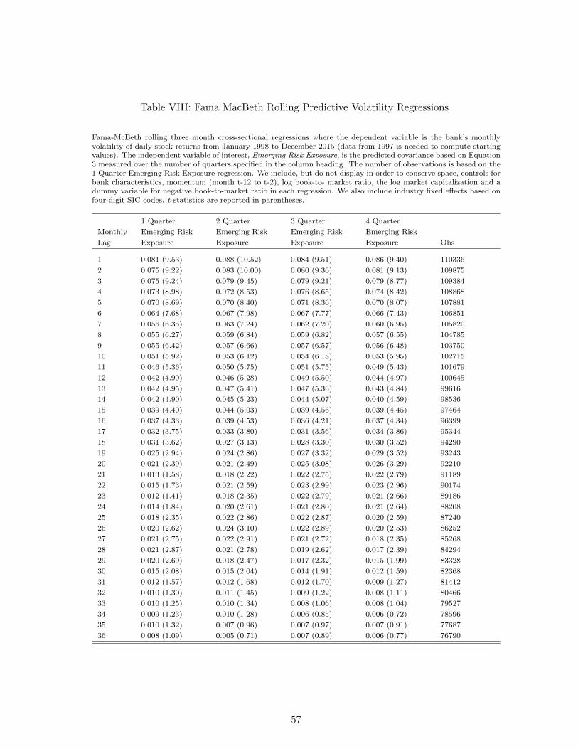
Table VIII: Fama MacBeth Rolling Predictive Volatility Regressions
Fama-McBeth rolling three month cross-sectional regressions where the dependent variable is the bank’s monthlyvolatility of daily stock returns from January 1998 to December 2015 (data from 1997 is needed to compute startingvalues). The independent variable of interest, Emerging Risk Exposure, is the predicted covariance based on Equation3 measured over the number of quarters specified in the column heading. The number of observations is based on the1 Quarter Emerging Risk Exposure regression. We include, but do not display in order to conserve space, controls forbank characteristics, momentum (month t-12 to t-2), log book-to- market ratio, the log market capitalization and adummy variable for negative book-to-market ratio in each regression. We also include industry fixed effects based onfour-digit SIC codes. t-statistics are reported in parentheses.
1 Quarter 2 Quarter 3 Quarter 4 Quarter
Monthly Emerging Risk Emerging Risk Emerging Risk Emerging Risk
Lag Exposure Exposure Exposure Exposure Obs
1 0.081 (9.53) 0.088 (10.52) 0.084 (9.51) 0.086 (9.40) 110336
2 0.075 (9.22) 0.083 (10.00) 0.080 (9.36) 0.081 (9.13) 109875
3 0.075 (9.24) 0.079 (9.45) 0.079 (9.21) 0.079 (8.77) 109384
4 0.073 (8.98) 0.072 (8.53) 0.076 (8.65) 0.074 (8.42) 108868
5 0.070 (8.69) 0.070 (8.40) 0.071 (8.36) 0.070 (8.07) 107881
6 0.064 (7.68) 0.067 (7.98) 0.067 (7.77) 0.066 (7.43) 106851
7 0.056 (6.35) 0.063 (7.24) 0.062 (7.20) 0.060 (6.95) 105820
8 0.055 (6.27) 0.059 (6.84) 0.059 (6.82) 0.057 (6.55) 104785
9 0.055 (6.42) 0.057 (6.66) 0.057 (6.57) 0.056 (6.48) 103750
10 0.051 (5.92) 0.053 (6.12) 0.054 (6.18) 0.053 (5.95) 102715
11 0.046 (5.36) 0.050 (5.75) 0.051 (5.75) 0.049 (5.43) 101679
12 0.042 (4.90) 0.046 (5.28) 0.049 (5.50) 0.044 (4.97) 100645
13 0.042 (4.95) 0.047 (5.41) 0.047 (5.36) 0.043 (4.84) 99616
14 0.042 (4.90) 0.045 (5.23) 0.044 (5.07) 0.040 (4.59) 98536
15 0.039 (4.40) 0.044 (5.03) 0.039 (4.56) 0.039 (4.45) 97464
16 0.037 (4.33) 0.039 (4.53) 0.036 (4.21) 0.037 (4.34) 96399
17 0.032 (3.75) 0.033 (3.80) 0.031 (3.56) 0.034 (3.86) 95344
18 0.031 (3.62) 0.027 (3.13) 0.028 (3.30) 0.030 (3.52) 94290
19 0.025 (2.94) 0.024 (2.86) 0.027 (3.32) 0.029 (3.52) 93243
20 0.021 (2.39) 0.021 (2.49) 0.025 (3.08) 0.026 (3.29) 92210
21 0.013 (1.58) 0.018 (2.22) 0.022 (2.75) 0.022 (2.79) 91189
22 0.015 (1.73) 0.021 (2.59) 0.023 (2.99) 0.023 (2.96) 90174
23 0.012 (1.41) 0.018 (2.35) 0.022 (2.79) 0.021 (2.66) 89186
24 0.014 (1.84) 0.020 (2.61) 0.021 (2.80) 0.021 (2.64) 88208
25 0.018 (2.35) 0.022 (2.86) 0.022 (2.87) 0.020 (2.59) 87240
26 0.020 (2.62) 0.024 (3.10) 0.022 (2.89) 0.020 (2.53) 86252
27 0.021 (2.75) 0.022 (2.91) 0.021 (2.72) 0.018 (2.35) 85268
28 0.021 (2.87) 0.021 (2.78) 0.019 (2.62) 0.017 (2.39) 84294
29 0.020 (2.69) 0.018 (2.47) 0.017 (2.32) 0.015 (1.99) 83328
30 0.015 (2.08) 0.015 (2.04) 0.014 (1.91) 0.012 (1.59) 82368
31 0.012 (1.57) 0.012 (1.68) 0.012 (1.70) 0.009 (1.27) 81412
32 0.010 (1.30) 0.011 (1.45) 0.009 (1.22) 0.008 (1.11) 80466
33 0.010 (1.25) 0.010 (1.34) 0.008 (1.06) 0.008 (1.04) 79527
34 0.009 (1.23) 0.010 (1.28) 0.006 (0.85) 0.006 (0.72) 78596
35 0.010 (1.32) 0.007 (0.96) 0.007 (0.97) 0.007 (0.91) 77687
36 0.008 (1.09) 0.005 (0.71) 0.007 (0.89) 0.006 (0.77) 76790
57
Related Documents