Dynamic Factor Models and Factor Augmented Vector Autoregressions Lawrence J. Christiano

Welcome message from author
This document is posted to help you gain knowledge. Please leave a comment to let me know what you think about it! Share it to your friends and learn new things together.
Transcript

Dynamic Factor Models and FactorAugmented Vector Autoregressions
Lawrence J. Christiano

Dynamic Factor Models and FactorAugmented Vector Autoregressions
• Problem:— the time series dimension of data is relatively short.— the number of time series variables is huge.
• DFM’s and FAVARs take the position:— there are many variables and, hence, shocks,— but, the principle driving force of all the variables may be justa small number of shocks.
• Factor view has a long-standing history in macro.— almost the definition of macroeconomics: a handfull of shocks- demand, supply, etc. - are the principle economic drivers.
— Sargent and Sims: only two shocks can explain a large fractionof the variance of US macroeconomic data.• 1977, “Business Cycle Modeling Without Pretending to HaveToo Much A-Priori Economic Theory,” in New Methods inBusiness Cycle Research, ed. by C. Sims et al., Minneapolis:Federal Reserve Bank of Minneapolis.

Why Work with a Lot of Data?
• Estimates of impulse responses to, say, a monetary policyshock, may be distorted by not having enough data in theanalysis (Bernanke, et. al. (QJE, 2005))
— Price puzzle:• measures of inflation tend to show transitory rise to a monetarypolicy tightening shock in standard (small-sized) VARs.
• One interpretation: Monetary authority responds to a signalabout future inflation that is captured in data not included in astandard, small-sized VAR.
• May suppose that ‘core inflation’is a factor that can only bededuced from a large number of different data.
• May want to know (as in Sargent and Sims), whether the datafor one country or a collection of countries can be characterizedas the dynamic response to a few factors.
Outline
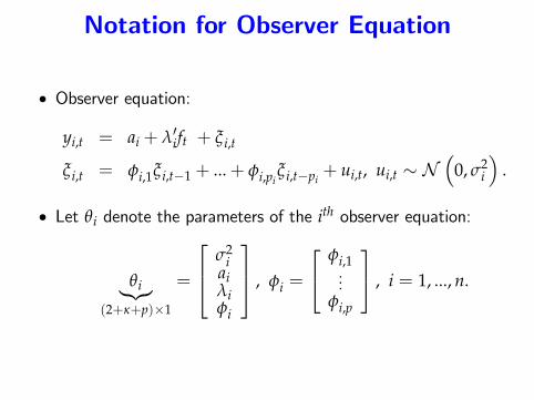
• Describe Dynamic Factor Model— Identification problem and one possible solution.
• Derive the likelihood of the data and the factors.• Describe priors, joint distribution of data, factors andparameters.
• Go for posterior distribution of parameters and factors.— Gibbs sampling, a type of MCMC algorithm.— Metropolis-Hastings could be used here, but would be veryineffi cient.
— Gibbs exploits power of Kalman smoother algorithm and thetype of fast ‘direct sampling’done with BVARS.
• FAVAR
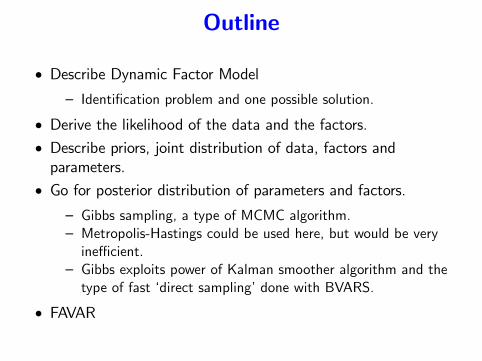
Dynamic Factor Model• Let Yt denote an n× 1 vector of observed data• Yt related to κ � n unobserved factors, ft, by measurement(or, observer) equation:
yi,t = ai +
vector of κ factor loadings︷︸︸︷λ′i ft +
idiosyncratic component of yi,t︷︸︸︷ξi,t .
• Law of motion of factors:
ft = φ0,1ft−1 + ...+ φ0,qft−q + u0,t, u0,t ∼ N (0, Σ0) .
• Idiosyncratic shock to yi,t (‘measurement error’):
ξi,t = φi,1ξ i,t−1 + ...+ φi,piξ i,t−pi
+ ui,t, ui,t ∼ N(
0, σ2i
).
• ui,t, i = 0, ..., n, drawn independently from each other and overtime.
• For convenience:
pi = p, for all i, q ≤ p+ 1.
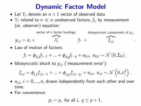
Notation for Observer Equation
• Observer equation:
yi,t = ai + λ′ift + ξi,t
ξi,t = φi,1ξ i,t−1 + ...+ φi,piξi,t−pi
+ ui,t, ui,t ∼ N(
0, σ2i
).
• Let θi denote the parameters of the ith observer equation:
θi︸︷︷︸(2+κ+p)×1
=
σ2i
aiλiφi
, φi =
φi,1...
φi,p
, i = 1, ..., n.
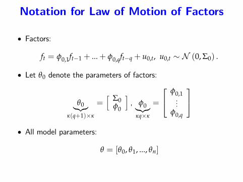
Notation for Law of Motion of Factors
• Factors:
ft = φ0,1ft−1 + ...+ φ0,qft−q + u0,t, u0,t ∼ N (0, Σ0) .
• Let θ0 denote the parameters of factors:
θ0︸︷︷︸κ(q+1)×κ
=[ Σ0
φ0
], φ0︸︷︷︸
κq×κ
=
φ0,1...
φ0,q
• All model parameters:
θ = [θ0, θ1, ..., θn]
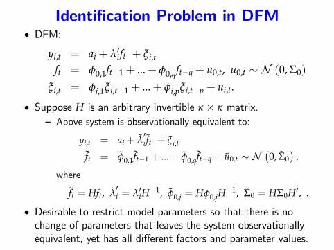
Identification Problem in DFM• DFM:
yi,t = ai + λ′ift + ξi,t
ft = φ0,1ft−1 + ...+ φ0,qft−q + u0,t, u0,t ∼ N (0, Σ0)
ξi,t = φi,1ξi,t−1 + ...+ φi,pξi,t−p + ui,t.
• Suppose H is an arbitrary invertible κ × κ matrix.— Above system is observationally equivalent to:
yi,t = ai + λ′i ft + ξ i,t
ft = φ0,1 ft−1 + ...+ φ0,q ft−q + u0,t ∼ N(0, Σ0
),
where
ft = Hft, λ′i = λ′iH
−1, φ0,j = Hφ0,jH−1, Σ0 = HΣ0H′, .
• Desirable to restrict model parameters so that there is nochange of parameters that leaves the system observationallyequivalent, yet has all different factors and parameter values.

Geweke-Zhou (1996) Identification• Note for any model parameterization, can always choose an Hso that Σ0 = Iκ.— Find C such that CC′ = Σ0 (there is a continuum of these),set H = C−1.
• Geweke-Zhou (1996) suggest the identifying assumption,Σ0 = Iκ.— But, this is not enough to achieve identification.— Exists a continuum of orthonormal matrices with property,
CC′ = Iκ.• Simple example: for κ = 2, for each ω ∈ [−π, π] ,
C =[
cos (ω) sin (ω)− sin (ω) cos (ω)
], 1 = cos2 (ω) + sin2 (ω)
— For each C, set H = C−1 = C′. That produces anobservationally equivalent alternative parameterization, whileleaving intact the normalization, Σ0 = Iκ, sinceHΣ0H′ = C′C = C−1C = Iκ.
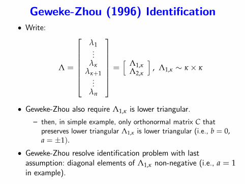
Geweke-Zhou (1996) Identification• Write:
Λ =
λ1...
λκλκ+1...
λn
=[ Λ1,κ
Λ2,κ
], Λ1,κ ∼ κ × κ
• Geweke-Zhou also require Λ1,κ is lower triangular.
— then, in simple example, only orthonormal matrix C thatpreserves lower triangular Λ1,κ is lower triangular (i.e., b = 0,a = ±1).
• Geweke-Zhou resolve identification problem with lastassumption: diagonal elements of Λ1,κ non-negative (i.e., a = 1in example).
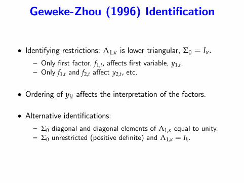
Geweke-Zhou (1996) Identification
• Identifying restrictions: Λ1,κ is lower triangular, Σ0 = Iκ.
— Only first factor, f1,t, affects first variable, y1,t.— Only f1,t and f2,t affect y2,t, etc.
• Ordering of yit affects the interpretation of the factors.
• Alternative identifications:— Σ0 diagonal and diagonal elements of Λ1,κ equal to unity.— Σ0 unrestricted (positive definite) and Λ1,κ = Ik.
Next:
• Move In direction of using data to obtain posterior distributionof parameters and factors.
• Start by going after the likelihood.
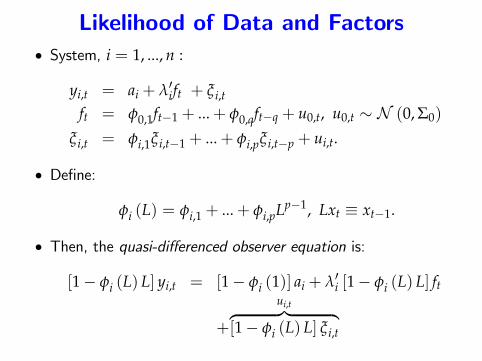
Likelihood of Data and Factors• System, i = 1, ..., n :
yi,t = ai + λ′ift + ξi,t
ft = φ0,1ft−1 + ...+ φ0,qft−q + u0,t, u0,t ∼ N (0, Σ0)
ξi,t = φi,1ξi,t−1 + ...+ φi,pξi,t−p + ui,t.
• Define:
φi (L) = φi,1 + ...+ φi,pLp−1, Lxt ≡ xt−1.
• Then, the quasi-differenced observer equation is:
[1− φi (L) L] yi,t = [1− φi (1)] ai + λ′i [1− φi (L) L] ft
+
ui,t︷ ︸︸ ︷[1− φi (L) L] ξi,t
Likelihood of Data and of Factors
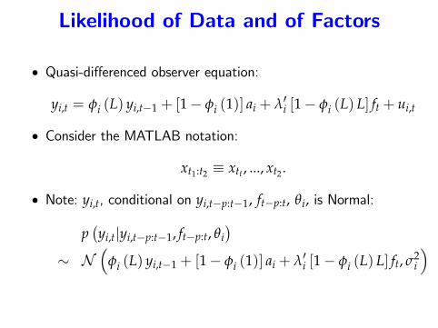
• Quasi-differenced observer equation:
yi,t = φi (L) yi,t−1 + [1− φi (1)] ai + λ′i [1− φi (L) L] ft + ui,t
• Consider the MATLAB notation:
xt1:t2 ≡ xtt , ..., xt2 .
• Note: yi,t, conditional on yi,t−p:t−1, ft−p:t, θi, is Normal:
p(yi,t|yi,t−p:t−1, ft−p:t, θi
)∼ N
(φi (L) yi,t−1 + [1− φi (1)] ai + λ′i [1− φi (L) L] ft, σ2
i
)
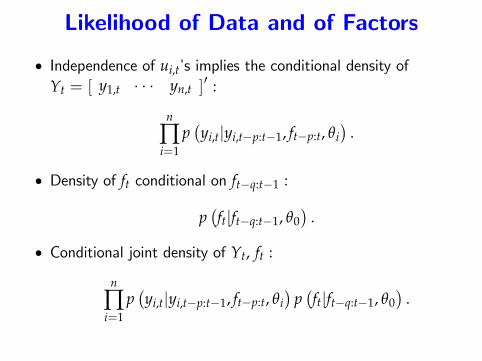
Likelihood of Data and of Factors
• Independence of ui,t’s implies the conditional density ofYt = [ y1,t · · · yn,t ]
′ :
n
∏i=1
p(yi,t|yi,t−p:t−1, ft−p:t, θi
).
• Density of ft conditional on ft−q:t−1 :
p(ft|ft−q:t−1, θ0
).
• Conditional joint density of Yt, ft :
n
∏i=1
p(yi,t|yi,t−p:t−1, ft−p:t, θi
)p(ft|ft−q:t−1, θ0
).
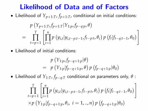
Likelihood of Data and of Factors• Likelihood of Yp+1:T, fp+1:T, conditional on initial conditions:
p(Yp+1:T, fp+1:T|Y1:p, fp−q:p, θ
)=
T
∏t=p+1
[n
∏i=1
p(yi,t|yi,t−p:t−1, ft−p:t, θi
)p(ft|ft−q:t−1, θ0
)]• Likelihood of initial conditions:
p(Y1:p, fp−q+1:p|θ
)= p
(Y1:p|fp−q+1:p, θ
)p(fp−q+1:p|θ0
)• Likelihood of Y1:T, fp−q:T conditional on parameters only, θ :
T
∏t=p+1
[n
∏i=1
p(yi,t|yi,t−p:t−1, ft−p:t, θi
)p(ft|ft−q:t−1, θ0
)]×p(Y1:p|fp−q+1:p, θi, i = 1, .., n
)p(fp−q+1:p|θ0
)

Joint Density of Data, Factors andParameters
• Parameter priors: p (θi) , i = 0, ..., n.• Joint density of Y1:T, fp−q:T, θ :
T
∏t=p+1
p(ft|ft−q:t−1, θ0
) n
∏i=1
p(yi,t|yi,t−p:t−1, ft−p:t, θi
)×[
n
∏i=1
p(yi,1:p|fp−q+1:p, θ
)p (θi)
]p(fp−q+1:p|θ0
)p (θ0)
• From here on, drop the density of initial observations.— if T is not too small, then has no effect on results.— BVAR lecture notes describe an example of how to not ignoreinitial conditions; for general discussion, see Del Negro andOtrok (forthcoming, RESTAT, "Dynamic Factor Models withTime-Varying Parameters: Measuring Changes in InternationalBusiness Cycles").

Outline
• Describe Dynamic Factor Model (done!)— Identification problem and one possible solution.
• Derive the likelihood of the data and the factors. (done!)• Describe priors, joint distribution of data, factors andparameters. (done!)
• Go for posterior distribution of parameters and factors.— Gibbs sampling, a type of MCMC algorithm.— Metropolis-Hastings could be used here, but would be veryineffi cient.
— Gibbs exploits power of Kalman smoother algorithm and thetype of fast ‘direct sampling’done with BVARS.
• FAVAR
Gibbs Sampling
• Idea is similar to what we did with the Metropolis-Hastingsalgorithm.

Gibbs Sampling versus Metropolis-Hastings• Metropolis-Hastings: we needed to compute the posteriordistribution of parameters, θ, conditional on the data.
— output of Metropolis-Hastings algorithm: sequence of values ofθ whose distribution corresponds to the posterior distributionof θ given the data:
P =[
θ(1) · · · θ(M)]
• Gibbs sampling algorithm: sequence of values of DFM modelparameters, θ, and unobserved factors, f , whose distributioncorresponds to the posterior distribution conditional on thedata:
P =[
θ(1) · · · θ(M)
f (1) · · · f (M)
].
Histogram of elements in individual rows of P representmarginal distribution of corresponding parameter or factor.

Gibbs Sampling Algorithm
• Computes sequence:
P =[
θ(1) · · · θ(M)
f (1) · · · f (M)
]= [ P1 · · · PM ] .
• Given Ps−1 compute Ps in two steps.
— Step 1: draw θ(s) given Ps−1 (direct sampling, using approachfor BVAR)
— Step 2: draw f (s) given θ(s) (direct sampling, based oninformation from Kalman smoother).

Step 1: Drawing Model Parameters
• Parameters, θ
observer equation: ai, λi
measurement error: σ2i , φi
law of motion of factors: φ0.
where the identification, Σ0 = I, is imposed.— Algorithm must be adjusted if some other identification is used.
• For each i :
— Draw ai, λi, σ2i from Normal-Inverse Wishart, conditional on
the φ(s−1)i ’s.
— Draw φi from Normal, given ai, λi, σ2i .
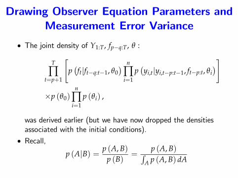
Drawing Observer Equation Parameters andMeasurement Error Variance
• The joint density of Y1:T, fp−q:T, θ :
T
∏t=p+1
[p(ft|ft−q:t−1, θ0
) n
∏i=1
p(yi,t|yi,t−p:t−1, ft−p:t, θi
)]
×p (θ0)n
∏i=1
p (θi) ,
was derived earlier (but we have now dropped the densitiesassociated with the initial conditions).
• Recall,
p (A|B) = p (A, B)p (B)
=p (A, B)∫
A p (A, B) dA

Drawing Observer Equation Parameters andMeasurement Error Variance
• Conditional density of θi obtained by dividing joint density byitself, after integrating out θi :
p(
θi|Y1:T, fp−q:T,{
θj}
j 6=i
)=
p(Y1:T, fp−q:T, θ
)∫θi
p(Y1:T, fp−q:T, θ
)dθi
∝ p (θi)T
∏t=p+1
p(yi,t|yi,t−p:t−1, ft−p:t, θi
)here, we have taken into account that the numerator anddenominator have many common terms.
• We want to draw θ(s)i from this posterior distribution for θi.
Gibbs sampling procedure:
— first, draw ai, λi, σ2i taking the other elements of θi from θ
(s−1)i .
— then, draw other elements of θi taking ai, λi, σ2i as given.
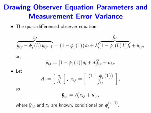
Drawing Observer Equation Parameters andMeasurement Error Variance
• The quasi-differenced observer equation:
yi,t︷ ︸︸ ︷yi,t − φi (L) yi,t−1 = (1− φi (1)) ai + λ′i
fi,t︷ ︸︸ ︷[1− φi (L) L] ft + ui,t,
or,yi,t = [1− φi (1)] ai + λ′i fi,t + ui,t.
• LetAi =
[ aiλi
], xi,t =
[(1− φi (1))
fi,t
],
soyi,t = A′ixi,t + ui,t,
where yi,t and xt are known, conditional on φ(s−1)i .

Drawing Observer Equation Parameters andMeasurement Error Variance
• From the Normality of the observer equation error:
p(yi,t|yi,t−p:t−1, ft−p:t, θi
)∝
1σi
exp
{−1
2
(yi,t −
[φi (L) yi,t−1 +A′ixi,t
])2
σ2i
}
=1σi
exp
{−1
2
(yi,t −A′ixi,t
)2
σ2i
}• Then,
T
∏t=p+1
p(yi,t|yi,t−p:t−1, ft−p:t, θi
)∝
1
σT−pi
exp
{−1
2
T
∑t=p+1
(yi,t −A′ixi,t
)2
σ2i
}.
Drawing Observer Equation Parameters andMeasurement Error Variance
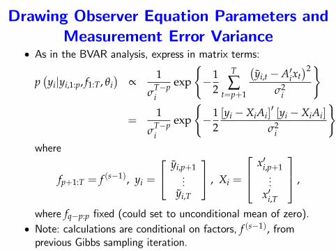
• As in the BVAR analysis, express in matrix terms:
p(yi|yi,1:p, f1:T, θi
)∝
1
σT−pi
exp
{−1
2
T
∑t=p+1
(yi,t −A′ixt
)2
σ2i
}
=1
σT−pi
exp
{−1
2[yi −XiAi]
′ [yi −XiAi]
σ2i
},
where
fp+1:T = f (s−1), yi =
yi,p+1...
yi,T
, Xi =
x′i,p+1...
x′i,T
,
where fq−p:p fixed (could set to unconditional mean of zero).• Note: calculations are conditional on factors, f (s−1), fromprevious Gibbs sampling iteration.

Including Dummy Observations• As in the BVAR analysis, T dummy equations are one way torepresent priors, p (θi) :
p (θi)T
∏t=p+1
p(yi,t|yi,t−p:t−1, ft−p:t, θi
)• Dummy observations (can include restriction that Λ1,κ is lowertriangular by suitable construction of dummies)
yi = XiAi + Ui,
Ui =
ui,1...
ui,T
.
• Stack the dummies with the actual data:
yi︸︷︷︸
(T−p+T)×1
=[ yi
yi
], Xi︸︷︷︸(T−p+T)×(1+κ)
=
[XiXi
].

Including Dummy Observations• As in BVAR:
p(yi|yi,1:p, f1:T, θi
)p(
λi, ai|σ2i
)∝
1
σT+T−pi
exp
−12
[y
i−XiAi
]′ [y
i−XiAi
]σ2
i
=
1
σT+T−pi
exp
{−1
2S+ (Ai −Ai)
′ X′iXi (Ai −Ai)
σ2i
}
=1
σT+T−pi
exp
{−1
2Sσ2
i
}exp
{−1
2(Ai −Ai)
′ X′iXi (Ai −Ai)
σ2i
}where
S =[y
i−XiAi
]′ [y
i−XiAi
], Ai =
(X′iXi
)−1 X′iyi.
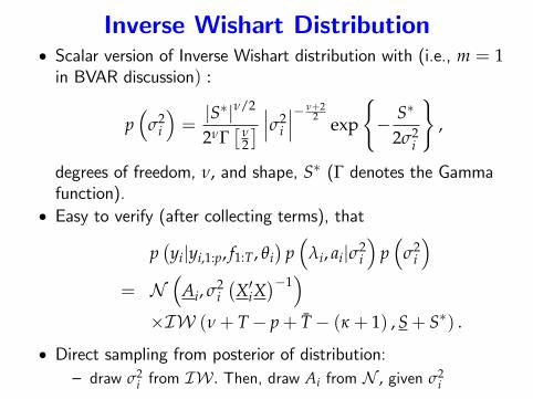
Inverse Wishart Distribution• Scalar version of Inverse Wishart distribution with (i.e., m = 1in BVAR discussion) :
p(
σ2i
)=|S∗|ν/2
2νΓ[
ν2
] ∣∣∣σ2i
∣∣∣− ν+22 exp
{− S∗
2σ2i
},
degrees of freedom, ν, and shape, S∗ (Γ denotes the Gammafunction).
• Easy to verify (after collecting terms), that
p(yi|yi,1:p, f1:T, θi
)p(
λi, ai|σ2i
)p(
σ2i
)= N
(Ai, σ2
i(X′iX
)−1)
×IW (ν+ T− p+ T− (κ + 1) , S+ S∗) .
• Direct sampling from posterior of distribution:— draw σ2
i from IW . Then, draw Ai from N , given σ2i

Draw Distributed Lag Coeffi cients inMeasurement Error Law of Motion
• Given λi, ai, σ2i , draw φi.
• Observer equation and measurement error process:
yi,t = ai + λ′ift + ξi,t
ξi,t = φi,1ξi,t−1 + ...+ φi,pξi,t−p + ui,t.
• Conditional on ai, λi and the factors, ξi,t can be computed from
ξi,t = yi,t − ai − λ′ift,
so the measurement error law of motion can be written,
ξi,t = A′ixi,t + ui,t, Ai = φi =
φi,1...
φi,p
, xi,t =
ξi,t−1...
ξi,t−p
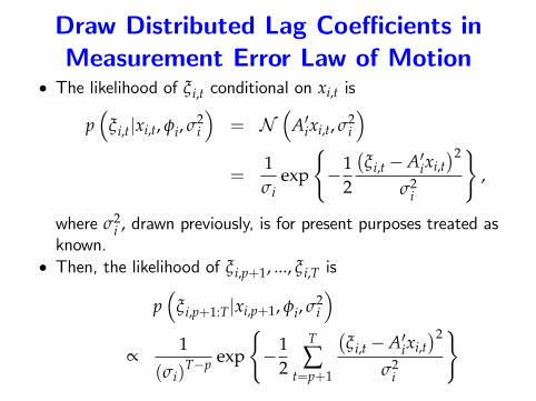
Draw Distributed Lag Coeffi cients inMeasurement Error Law of Motion
• The likelihood of ξi,t conditional on xi,t is
p(
ξi,t|xi,t, φi, σ2i
)= N
(A′ixi,t, σ2
i
)=
1σi
exp
{−1
2
(ξi,t −A′ixi,t
)2
σ2i
},
where σ2i , drawn previously, is for present purposes treated as
known.• Then, the likelihood of ξi,p+1, ..., ξi,T is
p(
ξi,p+1:T|xi,p+1, φi, σ2i
)∝
1
(σi)T−p exp
{−1
2
T
∑t=p+1
(ξi,t −A′ixi,t
)2
σ2i
}

Draw Distributed Lag Coeffi cients inMeasurement Error Law of Motion
T
∑t=p+1
(ξi,t −A′ixi,t
)2= [yi −XiAi]
′ [yi −XiAi] ,
where
yi =
ξi,p+1...
ξi,T
, Xi =
x′i,p+1...
x′i,T
,

Draw Distributed Lag Coeffi cients inMeasurement Error Law of Motion
• If we impose priors by dummies, then
p(
ξi,p+1:T|xi,p+1, φi, σ2i
)p (φi)
∝1
(σi)T−p exp
−12
[y
i−XiAi
]′ [y
i−XiAi
]σ2
i
,
where yiand Xi represents the stacked data that includes
dummies.• By Bayes’rule,
p(
φi|ξi,p+1:T, xi,p+1, φi, σ2i
)= N
(Ai, σ2
i(X′iX
)−1)
.
So, we draw φi from N(
Ai, σ2i(X′iX
)−1)
.
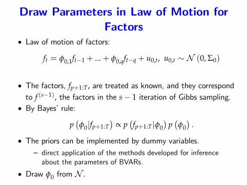
Draw Parameters in Law of Motion forFactors
• Law of motion of factors:
ft = φ0,1ft−1 + ...+ φ0,qft−q + u0,t, u0,t ∼ N (0, Σ0)
• The factors, fp+1:T, are treated as known, and they correspondto f (s−1), the factors in the s− 1 iteration of Gibbs sampling.
• By Bayes’rule:
p(φ0|fp+1:T
)∝ p
(fp+1:T|φ0
)p(φ0)
.
• The priors can be implemented by dummy variables.— direct application of the methods developed for inferenceabout the parameters of BVARs.
• Draw φ0 from N .
This Completes Step 1 of Gibbs Sampling
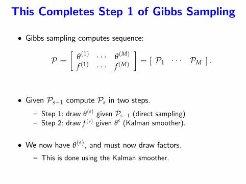
• Gibbs sampling computes sequence:
P =[
θ(1) · · · θ(M)
f (1) · · · f (M)
]= [ P1 · · · PM ] .
• Given Ps−1 compute Ps in two steps.
— Step 1: draw θ(s) given Ps−1 (direct sampling)— Step 2: draw f (s) given θs (Kalman smoother).
• We now have θ(s), and must now draw factors.
— This is done using the Kalman smoother.

Drawing the Factors• For this, we will put the DFM in the state-space form used tostudy Kalman filtering and smoothing.
— In that previous state space form, the measurement error wasassumed to be iid.
— We will make use of the fact that we have all modelparameters.
• The DFM:
yi,t = ai + λ′ift + ξi,t
ft = φ0,1ft−1 + ...+ φ0,qft−q + u0,t, u0,t ∼ N (0, Σ0)
ξi,t = φi,1ξi,t−1 + ...+ φi,pξi,t−p + ui,t.
• This can be put into our state space form (in which the errorsin the observation equation are iid) by quasi-differencing theobserver equation.

Observer Equation• Quasi differencing:
yi,t︷ ︸︸ ︷[1− φi (L) L] yi,t =
constant︷ ︸︸ ︷[1− φi (1)] ai + λ′i [1− φi (L) L] ft + ui,t
Then,
a =
[1− φi (1)] ai...
[1− φi (1)] ai
, yt =
y1,t...
yn,t
, Ft =
ft...
ft−p
H =
λ′1 −λ′1φ1,1 · · · −λ′1φ1,p...
.... . .
...λ′n −λ′nφn,1 · · · −λ′nφn,p
, ut =
u1,t...
un,t
yt = a+HFt + ut

Law of Motion of the State• Here, the state is denoted by Ft.• Law of motion:
ftft−1ft−2...
ft−p
=
φ0,1 φ0,2 · · · φ0,q 0κ×(p+1−q)Iκ 0κ · · · 0κ 0κ×(p+1−q)0 Iκ · · · 0κ 0κ×(p+1−q)...
.... . .
......
0 0 · · · Iκ 0κ×(p+1−q)
ft−1ft−2ft−3...
ft−1−p
+
u0,t
0κ×10κ×1...
0κ×1
• LoM:
Ft = ΦFt−1 + ut, ut ∼ N(
0κ(p+1)×1, V(p+1)κ×(p+1)κ
).

State Space Representation of the Factors• Observer equation:
yt = a+HFt + ut.
• Law of motion of state:
Ft = ΦFt−1 + ut.
• Kalman smoother provides:
P[Fj|y1, ..., yT
], j = 1, ..., T,
together with appropriate second moments.• Use this information to directly sample f (s) from theKalman-smoother-provided Normal distribution, completingstep 2 of the Gibbs sampler.

Factor Augmented VARs (FAVAR)• Favar’s are DFM’s which more closely resemble macro models.
— There are observables that act like ‘factors’, hitting allvariables directly
— Examples: the interest rate in the monetary policy rule,government spending, taxes, price of housing, world trade,international price of oil, uncertainty, etc.
• The measurement equation:
yi,t = ai + γiy0,t + λift + ξ i,t, i = 1, ..., n, t = 1, ..., T,
where y0,t and γi are m× 1 and 1×m vectors, respectively.• The vectors, y0,t and ft follow a VAR:[ ft
y0,t
]= Φ0,1
[ ft−1y0,t−1
]+ ...+Φ0,q
[ft−q
y0,t−q
]+ u0,t,
u0,t ∼ N (0, Σ0)
Literature on FAVARs is Large
• Initial paper: Bernanke and Boivin (2005QJE), "Measuring theEffects of Monetary Policy: A Factor-Augmented VectorAutoregressive (FAVAR) Approach."
• Intention was to correct problems with conventional VAR-basedestimates of the effects of monetary policy shocks.
• Include a large number of variables:— better capture the actual policy rule of monetary authorities,which look at lots of data in making their decisions.
— include a lot of variables so that the FAVAR can be used toobtain a comprehensive picture of the effects of a monetarypolicy shock on the whole economy.
— Bernanke, et al, include 119 variables in their analysis.

Literature on FAVARs is Large
• Literature is growing: "Large Bayesian Vector Autoregressions,"Banbura, Giannone, Reichlin (2010Journal of AppliedEconomicts), studies importance of including sectoral data toget better estimates of impulse response functions to policyshocks and a better estimate of their impact.
• DFM have been taken in interesting directions, more suitablefor multicountry settings, see, e.g., Canova and Ciccarelli(2013,ECB WP1507)
• Time varying FAVARs: Eickmeier, Lemke, Marcellino, "Classicaltime-varying FAVAR models - estimation, forecasting andstructural analysis," (2011Bundesbank Discussion Paper, no.04/2011). Argue that by allowing parameters to change overtime, get better forecasts and characterize how the economy ischanging.
Related Documents