Dynamic environmental modelling in GIS: 1. Modelling in three spatial dimensions

Research Article

Dynamic environmental modelling in GIS: 1. Modelling in three spatialdimensions

D. KARSSENBERG* and K. DE JONG

Department of Physical Geography, Faculty of Geosciences, Utrecht University, PO Box

80115, 3508 TC Utrecht, The Netherlands

(Received 18 February 2003; in final form 20 August 2004 )

Environmental modelling languages are programming languages developed for

building computer models simulating environmental processes. They come with

database and visualization routines for the data used in the models.

Environmental modelling languages provide the possibility to construct dynamic

models, also called forward models, which are simulations run forward in time,

where the state of the model at time t is defined as a function of its state in a time

step preceding t. Nowadays, these modelling languages can deal with simulations

in two spatial dimensions, but existing software does not support the

construction of models in three dimensions. We describe concepts of an

environmental modelling language supporting dynamic model construction in

two and three spatial dimensions. The lateral dimension is represented by gridded

maps, with a regular discretization, while the vertical dimension is represented by

an irregular discretization in voxels. Universal spatial functions are described

with these entities of the modelling language as input. Dynamic modelling

through time is possible by combining these functions in structured script

sections, providing a section, which is executed repetitively, representing the time

steps. The concepts of the language are illustrated with two example models, built

with a prototype of the language.

Keywords: Dynamic environmental modelling; Three spatial dimensions;

Python; Voxel; Spatio-temporal modelling

1. Introduction

In the environmental sciences, numerical computer models are a powerful means to

represent and communicate our understanding of the environment, and have a wide

application in predicting future changes in natural processes, often as a result of

human impact. Since most natural processes have spatial components that change

through time, these environmental computer models are typically spatial, with a

flow of information in two- or three-dimensional space, and over time. The

temporal behaviour is often simulated by dynamic modelling (Van Deursen 1995,

Gurney and Nisbet 1998), which uses rules of cause and effect. Dynamic modelling

involves a simulation which is run forward in time, where the state of a model at

time t+1 is defined as a deterministic or probabilistic function of its state in a

previous time step t. Examples of environmental models are found in research fields

*Corresponding author. E-mail: [email protected]

International Journal of Geographical Information Science

Vol. 19, No. 5, May 2005, 559–579

International Journal of Geographical Information ScienceISSN 1365-8816 print/ISSN 1362-3087 online # 2005 Taylor & Francis Group Ltd

http://www.tandf.co.uk/journalsDOI: 10.1080/13658810500032362

such as hydrology, ecology, crop science, soil science, sedimentology, climatology,

and glaciology.

Environmental models are currently mainly developed in general-purpose

programming languages (C++, Fortran, Python, Basic), technical computing

languages (MATLAB 2004) or graphical modelling languages (ModelMaker 2004,

STELLA 2004). General-purpose programming languages have the advantage that

these enable almost any program to be made, but they are not ideal for

environmental modellers who are not computer programmers mainly because the

level of thinking of these languages is too strongly related to specialized computer

science which may make model construction and modification cumbersome

(Karssenberg 2002). Although very powerful for numerical computation, technical

computing languages lack tools specific for environmental model construction, such

as standard spatial functions for watershed analysis, while coupling with databases

of Geographical Information Systems (GIS) is difficult. The graphical modelling

languages are very powerful for process modelling, but their non-spatial operators

do not provide the possibility of construction of models with spatial interaction.

Although not widely used, modelling languages included in many GIS are a

potential alternative for developing environmental models, since their concepts

provide advantages over the aforementioned tools, when applied for environmental

model construction (Karssenberg et al. 2001a, Karssenberg 2002). This is because

modelling languages in GIS:

1. provide functions in which commonly used spatial algorithms have been

pre-programmed;

2. provide these functions in a suitable way such that they can be glued together

in a model by a modeller using his or her understanding of environmental

processes rather than computer expertise;

3. provide generic tools for data input, database management and visualization

of data read and written by the model.

Nevertheless, GIS (ESRI 2004, Idris 2004) have so far failed to become important

tools for environmental model construction. Although they contain an extensive set

of spatial analysis tools, they are not tailored to dynamic spatial modelling requiring

optimization of sets of spatial functions executed in a sequence of time steps. In

addition, GIS do not provide interfaces specially developed for dynamic model

construction while they lack good tools for database management and visualization

of temporal data, such as rain time series or time series of vegetation patterns. Even

though GIS provide insufficient functionality for environmental model construc-

tion, the three conceptual advantages of GIS modelling languages over system

programming languages, as noted above, still exist. This has driven specialist

research groups to develop new modelling languages with sufficient functionality for

dynamic model building, embedded in GIS (Takeyama and Couclelis 1997, Pullar

2001, 2003, GRASS 2004, PCRaster 2004). For environmental model building, these

so-called environmental modelling languages now provide an alternative to system

programming languages. For instance, the PCRaster language (Van Deursen 1995,

Wesseling et al. 1996, PCRaster 2004) includes 120 spatial functions on gridded

maps. Building upon the natural language approach to modelling which was used by

Tomlin (1990), these languages use a mathematical notation of functions on maps:

ResultMap~function InputMapsð Þ ð1Þ

560 D. Karssenberg and K. De Jong

where function is a pre-programmed function, ResultMap is its output, and InputMaps

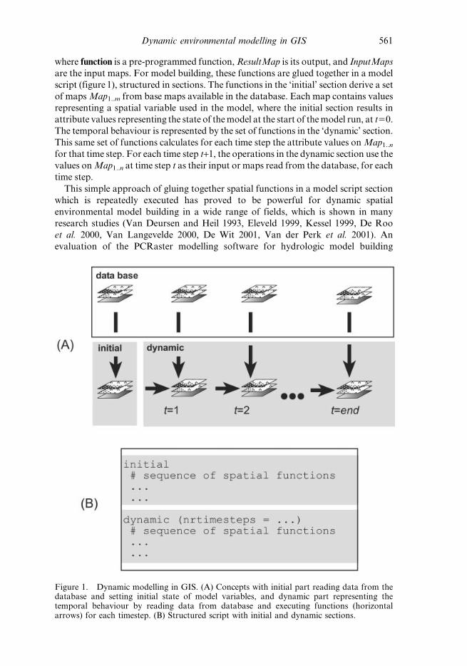
are the input maps. For model building, these functions are glued together in a model

script (figure 1), structured in sections. The functions in the ‘initial’ section derive a set

of maps Map1..m from base maps available in the database. Each map contains values

representing a spatial variable used in the model, where the initial section results in

attribute values representing the state of the model at the start of the model run, at t50.

The temporal behaviour is represented by the set of functions in the ‘dynamic’ section.

This same set of functions calculates for each time step the attribute values on Map1..n

for that time step. For each time step t+1, the operations in the dynamic section use the

values on Map1..n at time step t as their input or maps read from the database, for each

time step.

This simple approach of gluing together spatial functions in a model script section

which is repeatedly executed has proved to be powerful for dynamic spatial

environmental model building in a wide range of fields, which is shown in many

research studies (Van Deursen and Heil 1993, Eleveld 1999, Kessel 1999, De Roo

et al. 2000, Van Langevelde 2000, De Wit 2001, Van der Perk et al. 2001). An

evaluation of the PCRaster modelling software for hydrologic model building

Figure 1. Dynamic modelling in GIS. (A) Concepts with initial part reading data from thedatabase and setting initial state of model variables, and dynamic part representing thetemporal behaviour by reading data from database and executing functions (horizontalarrows) for each timestep. (B) Structured script with initial and dynamic sections.

Dynamic environmental modelling in GIS 561

(Karssenberg 2002), showed that its successful, wide application is mainly because

the pre-programmed functions can easily be glued together in a model script,

without the need for specialist programmers. But the same evaluation revealed many

weaknesses of environmental modelling languages. The main disadvantage lies in

the restricted functionality. In particular, the existing dynamic spatial environmental

modelling languages do not provide functionality for dynamic modelling in three

dimensions or for handling error propagation in dynamic modelling. This paper

focuses on modelling in three dimensions, while the second paper (Karssenberg and

De Jong 2005) of this series of two papers will deal with error propagation

modelling, building upon the language described here.

In addition to the two lateral dimensions, the third, vertical dimension, has an

obvious relevance in many dynamic environmental models. Three-dimensional

models are found in fields such as hydrology and soil science (Harbaugh and

McDonald 1996), sedimentology (Paola 2000), marine and lacustrine sciences

(Mason et al. 1994), crop and vegetation science (Song et al. 1997), and

meteorology. These models are generally developed in system programming

languages with a restricted application of GIS for visualization of model inputs

and outputs. Although three-dimensional GIS exist (EarthVision 2004, LYNX

2004), these are not used for dynamic modelling, since their functionality is focused

on database management, static (non-temporal) operations, such as volume

modelling, and visualization. There is a strong need to extend existing environ-

mental modelling languages, such as the PCRaster language described above, which

do provide functionality for dynamic modelling, with three-dimensional function-

ality, in addition to their two-dimensional functions on maps.

This paper describes how environmental modelling languages can be extended

with functionality for three-dimensional modelling and provides a prototype

environmental modelling language encapsulating these concepts, which is partly

developed using functions from the PCRaster software (Van Deursen 1995,

PCRaster 2004). In the first part of the paper, the application field of the developed

language is described. In the second part, the concepts of the language itself, its

entities and functions, and the syntax are described, while a prototype language

developed following these concepts is used in example models to illustrate its

application. Finally, the results are discussed.

2. Application field

2.1 Spatial dimension

The environmental modelling language is meant to simulate environmental

processes occurring within a three-dimensional block of material such as rock,

air, and/or vegetation. The focus is on spatially continuous phenomena. Processes

dealing with individuals moving in space, such as animals (Westervelt and Hopkins

1999, Bian 2000), are not dealt with, since this requires a different approach which is

beyond the scope of this research. Within the three-dimensional block, different

‘units’, such as rock layers, can be distinguished, each with specific properties for the

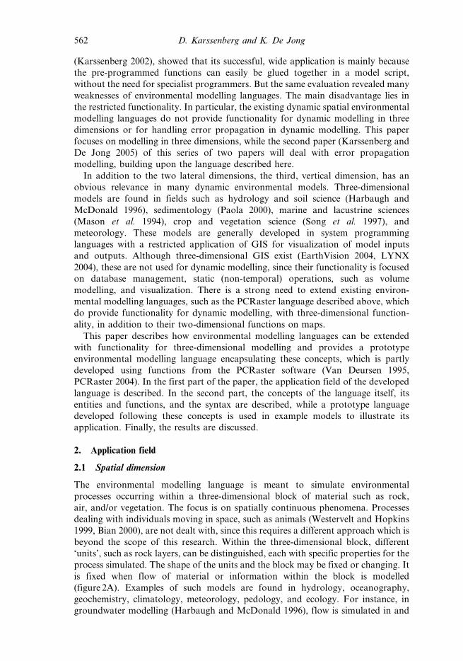
process simulated. The shape of the units and the block may be fixed or changing. It

is fixed when flow of material or information within the block is modelled

(figure 2A). Examples of such models are found in hydrology, oceanography,

geochemistry, climatology, meteorology, pedology, and ecology. For instance, in

groundwater modelling (Harbaugh and McDonald 1996), flow is simulated in and


between aquifers that mostly do not change in form and location in time spans

represented by the model.

The shape of the block will change when flow of material is simulated, resulting in

a change in shape of existing units, removal, or addition of units (figure 2B). Models

in fields such as geomorphology (Ahnert 1987), sedimentology (Tetzlaff and

Harbaugh 1989, Mackey and Bridge 1995), petroleum engineering (Karssenberg

et al. 2001b), and glaciology use a block of solid earth or ice where erosion and

deposition of material cause addition or abstraction of layers of material on the topside of the block. Processes such as compaction, faulting, and soil creep will cause a

change in shape of the units inside the block. In plant-growth models, the block of

units could represent a canopy, and growth of new layers of plants could extend the

block with new plant layers on the top side. Our focus is on changes in the shape of

the block by movement, deposition, or compression in vertical direction, ignoring

changes in the block in lateral direction, such as those caused by folding.

2.2 Temporal dimension

The focus is on dynamic environmental models that use the rules of cause and effect,

with a discretization of time in time steps. The state of the model variables, which

are attributes in one-, two-, or three-dimensional space, at time t+1 is defined by

their state at t and a function f. Similar descriptions can be found in Beck et al.

(1993), Van Deursen (1995), and Gurney and Nisbet (1998):

Z1::m tz1ð Þ~f Z1::m tð Þ, I1::n tð Þ, t, P1::lð Þ ð2Þ

The model variable(s) Z1..m belong to coupled processes and therefore have feedback

in time, for instance the stream water level. The model variable(s) I1..n are simple

inputs to the model, for instance incident rainfall in a runoff model and initial plantdistribution. Without I1..n, the model would represent a closed system. Boundary

conditions needed in a model are regarded here as an input Ii (t), too. The function f

with associated parameters P1..l models the change in the state of all model variables

over the time step t to t+1, and it can be either an update rule, explicitly specifying

the change of the state variable over the time slice (t, t+1), for instance a rule-based

function such as cellular automata (Toffoli 1989, Miyamoto and Sasaki 1997), or

alternatively a derivative of a differential equation describing the change of the state

variables as a continuous function (Gurney and Nisbet 1998). It may also includeprobabilistic rules when model behaviour is better described as a stochastic process,

which will be covered by the second paper.

Figure 2. (A) Processes in a three-dimensional block with a constant shape. (B) Processeschanging the shape of a three-dimensional block.


3. Entities of the language

3.1 Introduction

Entities of a language are the basic objects that carry the data, which are changed by

the modelling functions. Although the function f in equation (2) principally operates

at all locations in three-dimensional space, some processes typically represent only

the flow of material or information in the lateral direction, while other processes are

truly three-dimensional, such as groundwater flow. For this reason, two entities are

used in the language: two-dimensional ‘maps’, with a spatial discretization in ‘cells’,

and three-dimensional ‘blocks’, with a spatial discretization in ‘voxels’ (figure 3).

Both entities use the same discretization of the temporal dimension. In addition, the

discretization of the lateral spatial dimension is the same for maps and blocks. This

correspondence in discretization between maps and blocks guarantees efficient

exchange of information between the entities, in the same modelling environment.

3.2 Maps

A map discretizes the lateral space with a regular grid, as applied in many GIS.

Other possible approaches would be a vector approach or an irregular grid

discretization, but for the envisioned application field of the language (see section 2),

their advantages do not compensate for the advantages of a regular grid

discretization. The advantages of a regular grid are (1) its fixed neighbourhood

for each cell, which makes numerical solution schemes straightforward, (2) its

constant ‘support’ (Bierkens et al. 2000) of one grid cell, implying that cell values

and functions used in a model represent the average state or behaviour in an area of

a constant cell size, and (3) the availability of many numerical solution schemes,

including cellular automata. A vector approach would be needed for a change of

shape in the lateral direction (Raper 2000), caused for instance by folding inside the

three-dimensional block, but these processes are not meant to be modelled with the

language.

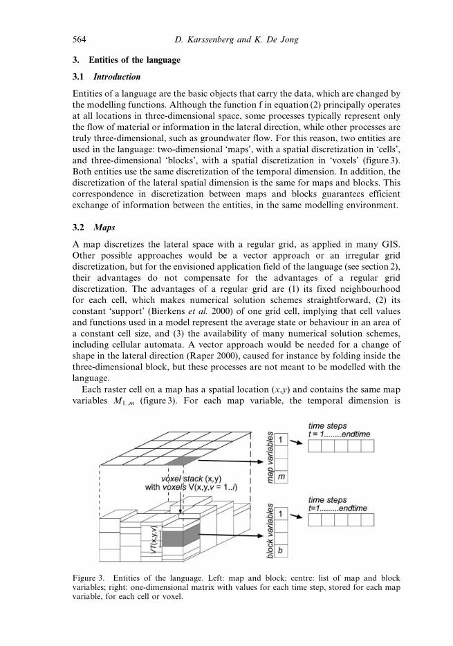
Each raster cell on a map has a spatial location (x,y) and contains the same map

variables M1..m (figure 3). For each map variable, the temporal dimension is

Figure 3. Entities of the language. Left: map and block; centre: list of map and blockvariables; right: one-dimensional matrix with values for each time step, stored for each mapvariable, for each cell or voxel.


represented by a one-dimensional array that is filled with cell values during a model

run. At the end of a model run, each field in this array contains an attribute value

for time step t, for the cell at (x,y). Each map variable is assigned a data type

(Boolean, nominal, scalar). Advantages of such a data-typing mechanism for spatial

data in a raster-modelling language were described by Van Deursen (1995) and

Wesseling et al. (1996).

3.3 Blocks

A block discretizes the lateral direction with the same regular grid of the maps used

in a model, providing a tight link between maps and blocks. For representing the

vertical direction in a block, there are at least three different approaches to choose

from. The first approach shown in figure 4A, using a regular discretization of the

vertical direction, has the advantage that each voxel has the same fixed set of

neighbouring cells, which provides a straightforward framework for implementing

spatial operations and visualization routines. In spite of this advantage, this

approach is not used here, because, (1) in often occurring cases of units with a very

small thickness, such as units formed by deposition of thin layers of sediment, a

small voxel thickness in the whole block would be required to represent these units,

resulting in an unacceptably large number of voxels; (2) the fixed vertical thickness

of voxels would result in unacceptably large numerical errors when a certain amount

of volume (sediment) is added on the top of the block, or in the case of a decrease in

thickness of existing units in the block (compaction); (3) exchange of data with

models that use another approach for discretization, such as groundwater flow

models (see below), becomes cumbersome and might involve resampling of voxels in

the vertical direction. It is obvious, though, that this regular discretization is still

powerful for many applications, which is shown by its use in models constructed

with the 3D module included in GRASS 5.0 (GRASS Development Team 2002,

Ciolli et al. 2004) and 3D-visualization software (OpenDX 2004, Slicer 2004).

The second approach (figure 4B), with a fixed number of voxels at each (x,y)

location, each with a different thickness, is efficient in representing laterally

continuous layers. As such, it is widely used in groundwater and unsaturated zone

flow modelling (Harbaugh and McDonald 1996, van Beek and van Asch 2004) or

meteorological modelling, but it is inadequate when layers are discontinuous, for

instance in the case of complex geological formations. The third approach with a

variable voxel thickness and a variable number of voxels per (x,y) location (figure 3)

is used here. It assumes a strong relation between the discretization and the

thickness of units mentioned in section 2.1, such as volumes with a specific rock

Figure 4. Discretization of the vertical dimension: (A) regular discretization and (B) fixednumber of voxels at each x,y location, each with a different thickness.


type, or trees with a certain property (see figure 1). Preferably, the thickness of a

voxel corresponds with the thickness of a certain unit at that location, although

exceptions may occur, when multiple voxels on top of each other are used to

represent the same unit. Note that the discretization in vertical direction is

analogous to a vector (polygon) representation of different units in two dimensions,

for instance applied on a soil type map, where the boundary between polygons is

defined by an abrupt change in a certain property. The same holds for boundaries

between voxels in the vertical direction, applied here. Advantages of this approach

are (1) an exact representation of the vertical position and thickness of units; (2) the

possibility of adding volumes of material or changing the thickness of units inside

the block within acceptable ranges of error; (3) minimization of the number of

voxels, since each unit is represented by one voxel, independent of the thickness of

the unit; and (4) generality, since the discretizations described in the first two

approaches above are subsets of this discretization. The main disadvantage of this

approach is that the number and location of neighbouring voxels will be different

for each voxel. As a result, spatial operations requiring a topology in three

dimensions will be complicated compared with spatial operations on a map with a

regular discretization. But this disadvantage is considered of minor importance,

mainly because the use of operations requiring a topology in three dimensions is

expected to be less frequent than the use of other operations, such as recoding voxel

values or operations requiring just the topology in vertical direction (vertical fluid

flow), which is constant for all voxels.

In the approach applied here, each location (x,y) on a regular grid contains a

stack of voxels with a temporally variable number of i voxels V(x,y,v), with v51 …

ix,y (figure 3). Each voxel V(x,y,v) has its own temporally variable voxel thickness

VT(x,y,v), and the bottom elevation of each voxel stack is the voxel stack bottom

VB(x,y). The top elevation of each voxel stack is VB(x,y) plus the sum of VT(x,y,v)

over v51 … ix,y. Each voxel contains the same block variables B1..b with an array

representation of attribute values in the temporal dimension also used for map

variables.

4. Functions of the language

4.1 General concepts

The function f (equation (2)) is represented by one or several functions on the map

or block entities of the modelling language. Functions are chosen, representing

universal functions on spatial entities, which can be applied in a wide range of

models. Many operations make sense in both the two-dimensional and three-

dimensional domain (think, for instance, of distance calculation). For this reason,

most functions work both on map and block entities, and the operation is modified

according to the input entity. For instance, a distance calculation function on a map

results in distances in two dimensions, given on a map, while the same calculation on

a block would result in a block entity with distances. This polymorphic behaviour

cannot be used for all functions, and a relatively small set of functions is provided

that work only on either maps or blocks. All functions check the data type of input

entities, and might change their behaviour according to the data type of the inputs

(Van Deursen 1995, Wesseling et al. 1996).

One group of functions results in a change of cell or voxel values on a map or in a

block, respectively. These are referred to as ‘functions on maps and blocks, no


change of form in spatial dimension’. In addition, a group of functions may change

the thickness of voxels or add or remove voxels from a block. These are referred to

as ‘functions on blocks, change of form in spatial dimension’. This group of

functions is not used for map entities, since the size and number of cells on a map are

constant.

4.2 Functions on maps and blocks, no change of form in spatial dimension

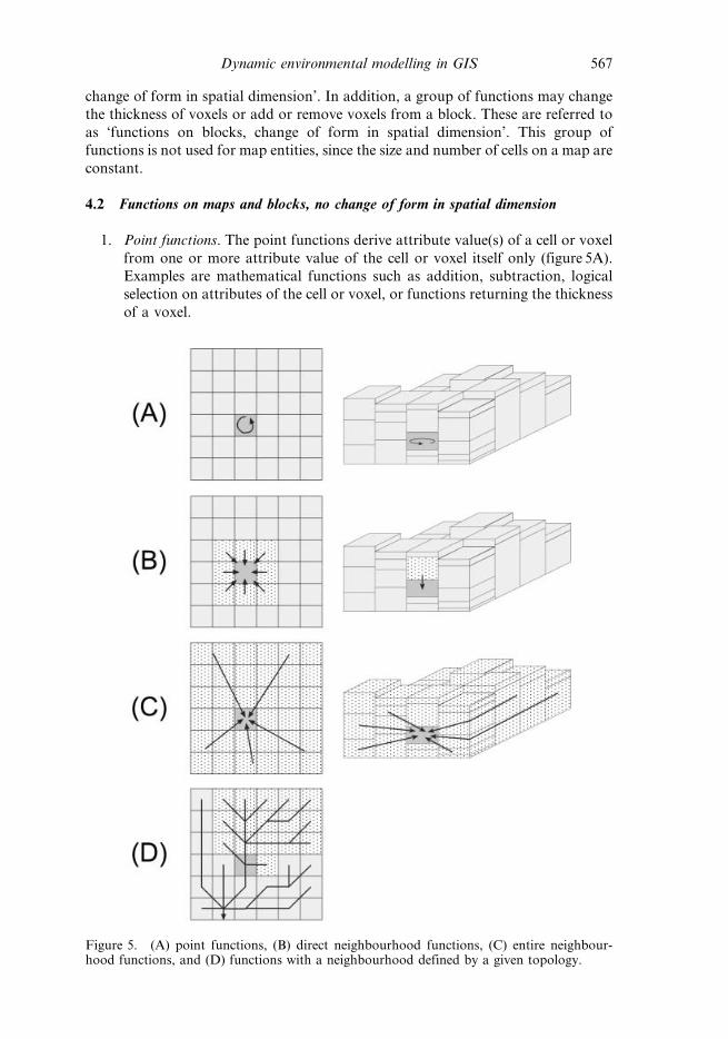
1. Point functions. The point functions derive attribute value(s) of a cell or voxel

from one or more attribute value of the cell or voxel itself only (figure 5A).

Examples are mathematical functions such as addition, subtraction, logical

selection on attributes of the cell or voxel, or functions returning the thickness

of a voxel.

Figure 5. (A) point functions, (B) direct neighbourhood functions, (C) entire neighbour-hood functions, and (D) functions with a neighbourhood defined by a given topology.


2. Direct neighbourhood functions. The direct neighbourhood functions

derive attribute value(s) of a cell or voxel from attribute value(s) in a

spatially restricted neighbourhood. Examples are two- or three-

dimensional moving filters, computing a new value of the centre cell or voxel

of a 2D or 3D window as a function of attribute values in the window.

An example of a direct neighbourhood function provided for blocks only

is a function assigning for each voxel an attribute value of the voxel

immediately above it (figure 5B, right), which could be used for simulating

infiltration.

3. Entire neighbourhood functions. The entire neighbourhood functions derive

attribute value(s) of a cell or voxel from attribute values(s) in all cells on a

map or block (figure 5C). All functions involving the solution of flow

equations in two or three dimensions belong to this group, e.g. groundwater

flow. Other functions belonging to this group are calculators of Euclidean or

relative distances to specific cells or voxels.

4. Functions with a neighbourhood defined by a given topology. This group of

functions derives for each cell or voxel an attribute value from attribute values

in a neighbourhood defined by an explicitly given topology. This topology

defines connections between cells or voxels. An example of such a topology is

a local drain direction network, representing flow directions over a map

(figure 5D). Functions using such a topology calculate catchment character-

istics such as catchment area or slope length, or transport material in a

downstream direction over the network (Van Deursen 1995).

4.3 Functions on blocks, change of form in spatial dimension

These are functions that change the form of the block as a whole, but only in the

vertical direction. This implies that the neighbourhood in the lateral direction

around voxels changes. The following groups are distinguished.

1. Top side block form functions. The top side block form functions remove or

add material at the top of the block, in a vertical direction. In the case of

addition of material (figure 6A), the attribute values of the volume added are

specified. Addition is done in two ways. If the added volume has attribute

properties similar to these of the voxel at the top of the block, the voxel

thickness of this existing voxel is increased. If the added volume is different

from the top voxel regarding attribute properties, a new voxel is added to

represent the addition. Removing volume means that voxels are completely or

partially removed at the top side of the block (figure 6B).

2. Inside block form functions. The inside block form functions change the

thickness of existing material inside the block, in the vertical direction

(figure 6C). This is done by changing the thickness of existing voxels inside the

block, without changing their attribute values. A change of thickness can be

caused by (1) a change of thickness of volume that is already inside the voxel

itself, e.g. compaction or decompaction of rock in situ, or compression of air,

and (2) addition or abstraction of volume from the voxel as a result of flow of

material between neighbouring voxels in lateral direction, e.g. soil creep.

3. Bottom side block form functions. The bottom side block form functions

change the location of volume in the block per x,y location, in a vertical

direction, as a result of change of elevation of the bottom of the block


(figure 6D). If the block represents the subsurface, it could be caused by faults

in the block.

4. Resampling functions. A resampling to another discretization in the vertical

dimension is done (1) when a regular discretization is needed for solving a

numerical algorithm in another function, e.g. for groundwater flow, while the

available data for that algorithm are available in a block with an irregular

discretization; or (2) when two blocks with a different discretization are

combined in a function that needs blocks with a corresponding discretization

as input, for instance when spatial statistics are calculated for different

realizations of a three-dimensional block.

5. Syntax

5.1 Introduction

The interface provided by the language for invoking and combining operations in a

model is mainly important for the activity of model building. While building a

Figure 6. Functions on blocks, change of form in spatial dimension: (A) top side block formfunctions, addition of material; (B) top side block form functions, removal of material; (C)inside block form functions; (D) bottom side block form functions.


model, the modeller is forced to work in this framework, and their way of thinking

will be influenced by it. Existing environmental modelling languages use either a

framework with a graphical representation (ESRI 2004, ModelMaker 2004,

STELLA 2004) or one with a textual representation of a model, being a

program or script (Pullar 2001, 2003, ESRI 2004, GRASS 2004, PCRaster 2004).

Since the graphical representation represents functions, and their inputs or outputs

as graphical entities, it has the advantage that it is very easy to use for

inexperienced users. While building a model, the researcher simply connects these

entities on the screen, resulting in a flow diagram similar to graphical representa-

tions of models often used in scientific reports (Forrester 1968). In spite of

this advantage of graphical modelling languages, a textual representation is

proposed here. This is mainly because a textual representation has the

advantage of an exact definition of the model in a model script, while the

functionality of a model represented by a flow diagram of a graphical representation

is not always unambiguous. Apart from this, experienced modellers are not expected

to prefer a graphical above a textual representation of a model, since they are

familiar with the mathematical notation that is often applied by textual modelling

languages.

The syntax of the language should follow common concepts of mathematical

notation and reasoning applied in scientific environmental modelling. The

natural language approach to modelling which was used by Tomlin (1990) is

convenient for simple spatial problems, but it cannot be used for more

complex modelling. The operations of the language are better represented as

functions with one or more inputs and one output, which can be nested. This

results in programs or scripts of a model that look similar to a theoretical,

mathematical description of the model, enhancing the readability of the model code.

In addition, the language should be understandable and easy to use for

environmental model builders, who do not necessarily need to be experienced

programmers. Technical details such as read/write definitions and storage allocation

should be avoided as much as possible, since they distract the modeller from

constructing the model.

5.2 Syntax of functions

From the line of thinking described above, a syntax for the functions is proposed

that follows algebraic notation (Wesseling et al. 1996):

Result~function Input1::nð Þ

with one of the functions of the language, function, having the input map or block

variables Input1..n, resulting in the output map or block variable Result. In most

cases, all input and output variables are either maps or blocks, although exceptions

occur, for instance when an input map adds information to a block, in which case

Input1..n are a block and a map, while the output is a block. The functions that make

sense both in two and three dimensions show polymorphic behaviour, which means

that their behaviour is adapted to the input(s). For instance, a point function sqrt

with a map variable as input calculates the square root for each cell on a map, giving

a map as Result, while the same function on a block would result in square roots for

each voxel in a block. In addition, all functions check the data type of their inputs,

and might change their behaviour depending on the data type of the input variable


(van Deursen 1995). The functions can be nested in a statement, where the result of

one or more functions function1..l is an input variable to another function:

Result~function function1::l Input1::mð Þ; Input1::nð Þ

5.3 Script structure

The functions are combined in a script or program, structured in sections (figure 7).

The concept of the script is similar to the concept of the script for dynamic

modelling in two dimensions (figure 1), although both maps and blocks can be used

now. Each section contains a list of operations that are sequentially executed. The

functions in the initial section are executed only once, at the start of the model run.

These read data from the database, generating map or block variables for the first

time step. The dynamic section, representing the temporal change, is a section that is

run for each time step. The functions in the dynamic section represent the change in

the state of model variables over one time step (equation (2)).

Figure 7. (A) Concepts and (B) modelling script for temporal, two- and three-dimensionalmodelling in GIS.


6. Example models

6.1 Dynamic model, no change of form in spatial dimension

A prototype implementation of the modelling language proposed here has been

created by extending an existing scripting language (Python 2004) with our 3D

modelling domain-specific data structures (maps and blocks) and functions. The

data structures and algorithms were written in a system programming language

(C++), using existing code from the PCRaster modelling language (Van Deursen

1995, PCRaster 2004). Data are read from and written to files. The dynamic model

given in table 1 simulates flow of water in the unsaturated zone of a soil, which is an

example of a model with a form of the block that is constant through time. For

reasons of clarity, it is a highly simplified example simulating only the key processes,

but it can easily be extended to a more realistic model. The functions in the initial

section, which are executed only once at the start of the model run, define the state

of the model at time step50. The first two statements create a block variable Type

(figure 8, left), containing the sediment type in three dimensions, and a block

variable T, which is the initial moisture content of the soil. These variables areassigned existing blocks, type.blk and t.blk, read from the database. The

residual moisture content (Tres, m3/m3) and the saturated moisture content (Tsat,m3/m3), which are, respectively, the minimum and maximum volume fraction ofwater the soil may contain, are assigned one value throughout the block. In reality,

these values will be different between soil types, but they are assumed to be constanthere. The fifth statement assigns a real length of 0.1 day to a variable TS

representing the length of a time step, which is used in the dynamic section.

The remaining statements in the initial section are all point functions on block

variables. The unsaturated conductivity (K, m/day) is assumed here to be constantthrough time, having the same value for all soil types, except the clay soil, which has

a lower value of unsaturated conductivity. The statement creating the block variable

Table 1. Modelling script for simulating infiltration of water (remarks are after a ‘#’, and allvariables are block variables).

initial

Type5’type.blk’ # block variable, sediment type

T5’t.blk’ # block var., initial moisture cont. (m3/m3)

Tres50.2 # residual moisture content (m3/m3)

Tsat50.5 # saturated moisture content (m3/m3)

TS50.1 # duration of a time step (days)

# unsaturated conductivity (m/day)

K5if((Type552) then 0.005 else 0.05)

# initial value of actual storage (m)

St5voxelthickness()*(T-Tres)

# maximum storage (m)

StMax5voxelthickness()*(Tsat-Tres)

dynamic (nrtimesteps5200)

# percolation (m per time step)

Perc5St*((K*TS)/voxelthickness())

# actual storage (m)

St5St-Perc+upper(Perc)

# relative degree of saturation (-)

Te5St/StMax


K nests an..(equals) function in an if..then..else function. If the condition

‘Type552’ is TRUE for a certain voxel, representing a voxel in Type with a class

value 2 (clay), the voxel is assigned an unsaturated conductivity of 0.005; if it isFALSE, it is assigned a value of 0.05 (figure 8). The next two statements calculate

the actual water storage (St, m) of a voxel, which is the actual amount of moveablewater in a voxel given as a slice of water, and the maximum storage (StMax, m).Both use the function voxelthickness() returning for each voxel its voxel thickness

(here in metres).

The sequence of functions in the dynamic section is run 200 times, representing

200 time steps of 0.1 day. The first function calculates for each voxel the amount of

water (Perc, m per time step) that percolates to its underlying voxel. According to

the theory of unsaturated flow, this is a function of the unsaturated conductivity, the

distance of transport (voxel thickness) and the length of a timestep. The next

statement updates the actual storage (St, m) for each voxel by subtracting from theactual storage the amount of water that flows out of the voxel to its underlying voxel(Perc), and adding the percolation from the overhead voxel. The latter is done with

the upper function, which assigns to each voxel the value from its overhead voxel.

The last function in the dynamic calculates for each time step the resulting relative

degree of saturation, for which the results are shown for three time steps in figure 9.

It should be noted that this simplified model script can be extended with a surface

water component (Karssenberg 2002) representing with map variables and functions

the process of rainfall, interception, surface storage, and runoff, providing water

inputs to the upper voxels of the model component shown here. In addition,

saturated flow in deeper soil layers can be simulated by extending the model script.

6.2 Dynamic model, change of form in spatial dimension

Another example model was made, predicting the three-dimensional architecture of

river deposits, simulating the formation of a series of deposits formed by the river

channel, with associated overbank deposits next to these channel belt deposits.

Table 2 gives the script for a simplified version of the model described by Mackey

and Bridge (1995), rewritten in PCRaster (Karssenberg et al. 2001b). Note that all

variables in table 2 are maps, apart from LithBlock, which is a block variable.Figure 10 gives the set of maps created for one time step in the model, representing

the formation of one channel belt, and its associated deposits.

Figure 8. Input block variable Type (left) and resulting block variable K (right) of thefunction K5if((Type552) then 0.005 else 0.05).


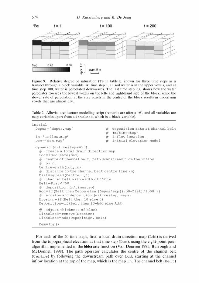
For each of the 20 time steps, first, a local drain direction map (Ldd) is derived

from the topographical elevation at that time step (Dem), using the eight-point pouralgorithm implemented in the lddcreate function (Van Deursen 1995, Burrough and

McDonnell 1998). The path operator calculates the centre of the channel belt

(Centre) by following the downstream path over Ldd, starting at the channelinflow location at the top of the map, which is the map In. The channel belt (Belt)

Table 2. Alluvial architecture modelling script (remarks are after a ‘#’, and all variables aremap variables apart from LithBlock, which is a block variable).

initial

Depos5’depos.map’ # deposition rate at channel belt

# (m/timestep)

In5’inflow.map’ # inflow location

Dem5’dem.map’ # initial elevation model

dynamic (nrtimesteps520)

# create a local drain direction map

Ldd5lddcreate(Dem)

# centre of channel belt, path downstream from the inflow

# point

Centre5path(Ldd,In)

# distance to the channel belt centre line (m)

Dist5spread(Centre,0,1)

# channel belt with width of 1500m

Belt5Dist,750

# deposition (m/timestep)

Add5if(Belt then Depos else (Depos*exp((750-Dist)/1500)))

# erosion and deposition (m/timestep, maps)

Erosion5if(Belt then 10 else 0)

Deposition5if(Belt then 10+Add else Add)

# adjust thickness of block

LithBlock5remove(Erosion)

LithBlock5add(Deposition, Belt)

Dem5top()

Figure 9. Relative degree of saturation (Te in table 1), shown for three time steps as atransect through a block variable. At time step 1, all soil water is in the upper voxels, and attime step 100, water is percolated downwards. The last time step 200 shows how the waterpercolates towards the lowest voxels on the left- and right-hand side of the block, while theslower rate of percolation at the clay voxels in the centre of the block results in underlyingvoxels that are almost dry.


Figure 10. Alluvial architecture model, one realization at time step 20; the flow direction isfrom top to bottom on the maps. (A) Zoomed area of local drain direction map (Ldd intable 2); (B) channel belt centre cells (Centre); (C) distance to the channel belt centre (Dist);(D) channel belt (Belt); (E) deposition (Add, m/time step); and (F), topographical elevation(Dem, m) after erosion and deposition, used for the next time step.


consists of all cells with a distance less than half the width of the channel belt, whichis 750m in this case. This map is calculated by the two spread operations, which

calculate the distance from the TRUE cells on Centre, resulting in the map Dist,and a ‘less than’ (0) function operating on Dist. The pattern of deposition (Add) is

derived from the channel belt map, assuming a negative exponential decrease indeposition with distance from the channel belt. The variable LithBlock is thethree-dimensional block with the lithology, containing channel belt deposits in a

matrix of overbank deposits. This block is for each time step updated by the remove

function, resulting in incision in the old deposits at the location of the channel belt,

and the add function, resulting in filling of this incised band with channel belt

deposits, and additional deposition next to the channel. Figure 11 gives a three-

dimensional output of one realization of the model. Since deposition decreases with

downstream distance, each new channel belt diverges from the previous one at the

inflow location, which is called nodal avulsion (Mackey and Bridge 1995).

7. Discussion and conclusions

The goal of this study is to provide new concepts to extent existing dynamic spatial

environmental modelling languages with functionality for modelling in three spatial

dimensions. It was possible to implement an example model with the prototype

language, built according to these concepts. This does not mean that we have arrived

at a final version of the language. Many steps need to be taken before a new grown-

up tool for construction of multi-dimensional models becomes available. Below, a

short discussion is given of the main weaknesses of the current prototype language.

Compared with two-dimensional static or dynamic models, the amount of data

related to the type of models worked with here is enormous, since three spatial

Figure 11. Example output of alluvial architecture model, timestep 20, three-dimensionalpicture of channel belt deposits, LithBlock in table 2. Inflow point at top of image: the lateralextension corresponds to figure 10, and the thickness of the individual channel belts is 10m.


dimensions need to be represented. This is a problem both from the data-storage

point of view and with regard to the run times of models. Since this paper focuses on

the concepts of the language and its entities, these problems are not dealt with in theprototype language. So, optimization routines need to be developed. Regarding data

storage, the main optimization possible is to reduce the number of voxels in three-

dimensional blocks until acceptable degrees of resolution are obtained by built-in

resampling. This would also decrease the run times of the models, since the data

volume decreases.

In order to be useful for environmental researchers, the language needs to match

their way of thinking. It should be possible for researchers to understand the

concepts intuitively. Although different approaches are possible, the approach

regarding the script structure and syntax of the functions used here is similar to

concepts of other existing environmental modelling languages (PCRaster 2004).

Since these languages have a wide application, it is expected that researchers will

understand the concepts of the language proposed here, too.

The PCRaster research and development team will release a PCRaster Python

extension based upon the prototype language described in this paper. Information is

available at http://pcraster.geo.uu.nl

Acknowledgements

We wish to thank Peter Burrough, Cees Wesseling, Willem van Deursen,

Marc Bierkens, and Edzer Pebesma for giving many inputs to the research

described. This research was supported in part by EC grant Eurodelta, EVK3-

CT2001–20001.

ReferencesAHNERT, F., 1987, Process-response models of denudation at different spatial scales. Catena

Supplement, 10, pp. 31–50.

BECK, M.B., JAKEMAN, A.J. and MCALEER M.J., 1993, Construction and evaluation of

models of environmental systems. In M.B. Beck, A.J. Jakeman and M.J. McAleer

(Eds.), Modelling change in environmental systems (New York: Wiley), pp. 3–35.

BIAN, L., 2000, Object-oriented representation for modelling mobile objects in an

aquatic environment. International Journal of Geographical Information Science, 14,

pp. 603–623.

BIERKENS, M.F.P., FINKE, P.A. and DE WILLIGEN, P., 2000, Upscaling and Downscaling

Methods for Environmental Research (Dordrecht: Kluwer).

BURROUGH, P.A. and MCDONNELL, R.A., 1998, Principles of Geographical Information

Systems (Oxford: Oxford University Press).

CIOLLI, M., DE FRANCESCHI, M., REA, R., VITTI, A., ZARDI, D. and ZATELLI, P., 2004,

Development and application of 2D and 3D GRASS modules for simulation of

thermally driven slope winds. Transactions in GIS, 8, pp. 191–209.

DE ROO, A.P.J., WESSELING, C.G. and VAN DEURSEN, W.P.A., 2000, Physically based river

basin modelling within a GIS; the LISFLOOD model. Hydrological Processes, 14, pp.

1981–1992.

DE WIT, M., 2001, Nutrient fluxes at the river basin scale. I: the PolFlow model. Hydrological

Processes, 15, pp. 743–759.

EARTHVISION, 2004, EarthVision, Dynamic Graphics, Inc. Available online at: http://

www.dgi.com (accessed February 24th 2005).

ELEVELD, M., 1999, Exploring Coastal Morphodynamics of Ameland (the Netherlands) with

Remote Sensing Monitoring Techniques and Dynamic Modelling in GIS (Amsterdam:

Universiteit van Amsterdam).


ESRI, 2004, Environmental Systems Research Institute. Available online at: http://

www.esri.com/ (accessed February 24th, 2005).

FORRESTER, J.W., 1968, Principles of systems. Text and workbook chapters 1 through 10

(Cambridge, MA: Wright-Allen Press).

GRASS, 2004, Available online at: http://www.geog.uni-hannover.de/grass/ (accessed February

24th, 2005).

GRASS DEVELOPMENT TEAM, 2002, GRASS 5.0 User’s Manual, Trento, Italy, ITC-irst.

Available online at: http://grass.itc.it/gdp/html_grass5 (accessed February 24th, 2005).

GURNEY, W.S.C. and NISBET, R.M., 1998, Ecological Dynamics (New York: Oxford

University Press).

HARBAUGH, A.W. and MCDONALD, M.G., 1996, User’s documentation for MODFLOW-96,

an update to the U.S. Geological Survey Modular Finite-Difference Ground-Water Flow

Model (Denver, CO: US Geological Survey).

IDRISI 2004. Available online at: http://www.clarklabs.org (accessed February 24th, 2005).

KARSSENBERG, D., 2002, The value of environmental modelling languages for building

distributed hydrological models. Hydrological Processes, 16, pp. 2751–2766.

KARSSENBERG, D. and DE JONG, K., 2005, Dynamic environmental modelling in GIS: 2.

Modelling error propagation. International Journal of Geographic Information

Science, in press.

KARSSENBERG, D., BURROUGH, P.A., SLUITER, R. and DE JONG, K., 2001, The PCRaster

software and course materials for teaching numerical modelling in the environmental

sciences. Transactions in GIS, 5, pp. 99–110.

KARSSENBERG, D., TORNQVIST, T. and BRIDGE, J.S., 2001, Conditioning a process-based

model of sedimentary architecture to well data. Journal of Sedimentary Research, 71,

pp. 868–879.

KESSEL, G., 1999, Biological control of Botrytis spp. by Ulocladium atrum, an ecological

analysis (Wageningen: Wageningen University).

LYNX, 2004, Lynx Geosystems, 2004. Available online at: http://www.lynxgeo.com (accessed

February 24th, 2005).

MACkEY, S.D. and BRIDGE, J.S., 1995, Three-dimensional model of alluvial stratigraphy:

theory and application. Journal of Sedimentary Research, B65, pp. 7–31.

MASON, D.C., O’CONNALL A. and BELL, S.B.M., 1994, Handling four-dimensional geo-

referenced data in environmental GIS. International Journal of Geographical

Information Systems, 8, pp. 191–215.

MATLAB 2004. Available online at: http://www.mathworks.com (accessed February 24th,

2005).

MIYAMOTO, H. and SASAKI, S., 1997, Simulating lava flows by an improved cellular automata

method. Computers & Geosciences, 23, pp. 283–292.

MODELMAKER, 2004. Available online at: http://www.modelkinetix.com/modelmaker

(accessed February 24th, 2005).

OPENDX 2004. Available online at: http://www.research.ibm.com/dx/ (accessed February

24th, 2005).

PAOLA, C., 2000, Quantitative models of sedimentary basin filling. Sedimentology,

47(Supplement 1), pp. 121–178.

PCRASTER 2004. Available online at: http://pcraster.geo.uu.nl (accessed February 24th, 2005).

PULLAR, D., 2001, MapScript: a map algebra programming language incorporating

neighborhood analysis. Geoinformatica, 5, pp. 145–163.

PULLAR, D., 2003, Simulation modelling applied to runoff modelling using MapScript.

Tranactions in GIS, 7, pp. 267–283.

PYTHON, 2004. Python language. Available online at: http://www.python.org (accessed

February 24th, 2005).

RAPER, J., 2000, Multidimensional Geographic Information Science (London: Taylor &

Francis).

SLICER, 2004. Available online at: http://www.slicer.org (accessed February 24th, 2005).


SONG, B., CHEN, J., DESANKER, P.V., REED, D.D., BRADSHAW, G.A. and FRANKLIN, J.F.,

1997, Modeling canopy structure and heterogeneity across scales: from crowns to

canopy. Forest Ecology and Management, 96, pp. 217–229.

STELLA, 2004. Available online at: http://www.iseesystems.com (accessed February 24th,

2005).

TAKEYAMA, M. and COUCLELIS, H., 1997, Map dynamics: integrating cellular automata and

GIS through Geo-Algebra. International Journal of Geographical Information Science,

11, pp. 73–91.

TETZLAFF, D.M. and HARBAUGH, J.W., 1989, Simulating Clastic Sedimentation (New York:

Van Nostrand Reinhold).

TOFFOLI, T., 1989, Cellular Automata Machines (Cambridge, MA: MIT Press).

TOMLIN, C.D., 1990, Geographic Information Systems and Cartographic Modelling

(Englewood Cliffs, NJ: Prentice-Hall).

VAN BEEK, L.P.H. and VAN ASCH, T.W.J., 2004, Regional assessment of the effects of land-

use change on landslide hazard by means of physically based modelling. Natural

Hazards, 31, pp. 289–304.

VAN DER PERK, M., BUREMA, J.R., BURROUGH, P.A., GILLET, A.G. and VAN DER

MEER, M.B., 2001, A GIS-based environmental decision support system to assess

the transfer of long-lived radiocaesium through food chains in areas contaminated by

the Chernobyl accident. International Journal of Geographical Information Science, 15,

pp. 43–64.

VAN DEURSEN, W.P.A., 1995, Geographical Information Systems and Dynamic Models

(Utrecht: Koninklijk Nederlands Aardrijkskundig Genootschap/Faculteit Ruimtelijke

Wetenschappen, Universiteit Utrecht).

VAN DEURSEN, W.P.A. and HEIL, G.W., 1993, Analysis of heathland dynamics using a spatial

distributed GIS model. Scripta Geobotanica, 21, pp. 17–28.

VAN LANGEVELDE, F., 2000, Scale of habitat connectivity and colonization in fragmented

nuthatch populations. Ecography, 23, pp. 614–622.

WESSELING, C.G., KARSSENBERG, D., VAN DEURSEN, W.P.A. and BURROUGH, P.A., 1996,

Integrating dynamic environmental models in GIS: the development of a Dynamic

Modelling language. Transactions in GIS, 1, pp. 40–48.

WESTERVELT, J.D. and HOPKINS, L.D., 1999, Modeling mobile individuals in

dynamic landscapes. International Journal of Geographical Information Science, 13,

pp. 191–208.


Dynamic environmental modelling in GIS: 1. Modelling in three spatial dimensions

Documents