Dynamic Effects of Feedback Control Robert Stengel Robotics and Intelligent Systems MAE 345, Princeton University, 2017 Copyright 2017 by Robert Stengel. All rights reserved. For educational use only. http://www.princeton.edu/~stengel/MAE345.html • Inner, Middle, and Outer Feedback Control Loops • Step Response of Linear, Time- Invariant (LTI) Systems • Position and Rate Control • Transient and Steady-State Response to Sinusoidal Inputs 1 Outer-to-Inner-Loop Control Hierarchy • Inner Loop – Small Amplitude – Fast Response – High Bandwidth • Middle Loop – Moderate Amplitude – Medium Response – Moderate Bandwidth • Outer Loop – Large Amplitude – Slow Response – Low Bandwidth • Feedback – Error between command and feedback signal drives next inner-most loop 2

Welcome message from author
This document is posted to help you gain knowledge. Please leave a comment to let me know what you think about it! Share it to your friends and learn new things together.
Transcript
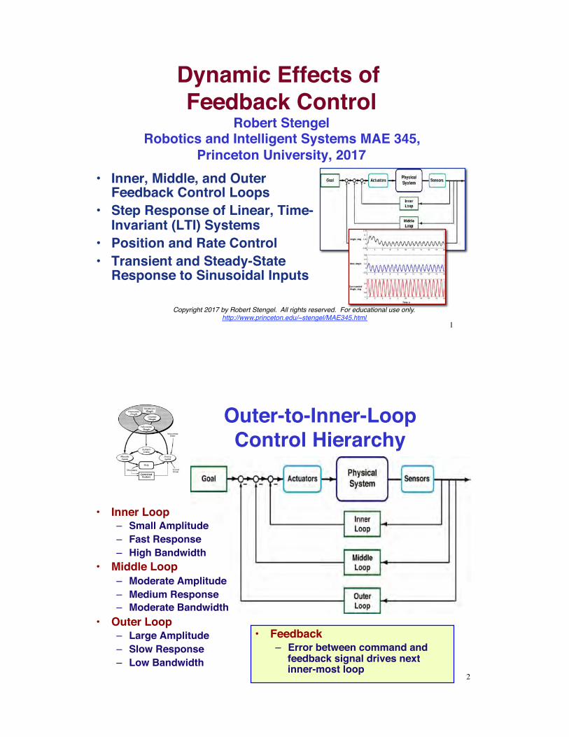
Dynamic Effects of Feedback Control !
Robert Stengel! Robotics and Intelligent Systems MAE 345,
Princeton University, 2017
Copyright 2017 by Robert Stengel. All rights reserved. For educational use only.http://www.princeton.edu/~stengel/MAE345.html
•! Inner, Middle, and Outer Feedback Control Loops
•! Step Response of Linear, Time-Invariant (LTI) Systems
•! Position and Rate Control•! Transient and Steady-State
Response to Sinusoidal Inputs
1
Outer-to-Inner-Loop Control Hierarchy
•! Inner Loop–! Small Amplitude–! Fast Response–! High Bandwidth
•! Middle Loop–! Moderate Amplitude–! Medium Response–! Moderate Bandwidth
•! Outer Loop–! Large Amplitude–! Slow Response–! Low Bandwidth
•! Feedback–! Error between command and
feedback signal drives next inner-most loop
2
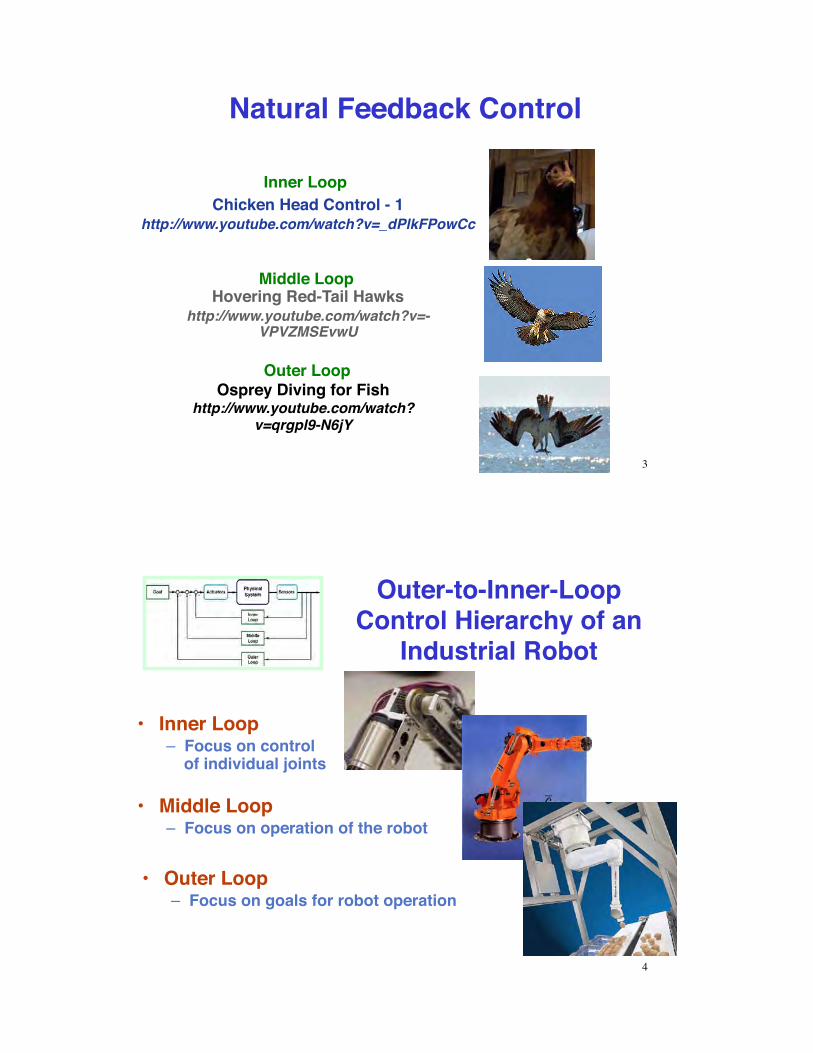
Natural Feedback Control
Chicken Head Control - 1http://www.youtube.com/watch?v=_dPlkFPowCc
Osprey Diving for Fishhttp://www.youtube.com/watch?
v=qrgpl9-N6jY
Inner Loop
Middle Loop
Outer Loop
Hovering Red-Tail Hawkshttp://www.youtube.com/watch?v=-
VPVZMSEvwU
3
Outer-to-Inner-Loop Control Hierarchy of an
Industrial Robot
•! Inner Loop–! Focus on control
of individual joints
•! Middle Loop–! Focus on operation of the robot
•! Outer Loop–! Focus on goals for robot operation
4

Inner-Loop Feedback Control
Single-Input/Single-Output Example, with forward and feedback control logic ( compensation )
Feedback control design must account for actuator-system-sensor dynamics
5
Thermostatic Temperature Control
•! Dynamics–! Delays–! Dead Zones–! Saturation–! Coupling
•! External Effects–! Solar Radiation–! Air Temperature–! Wind–! Rain, Humidity
•! Structure–! Layout–! Insulation–! Circulation–! Multiple Spaces
... all controlled by a simple (but nonlinear) on/off switch6

Thermostat Control Logic
e(t) = yc(t)! y(t) = uc(t)! ub (t)< Thermostat >
u(t) =1(on), e(t) > 00 (off ), e(t) " 0
#$%
&%
•! Control Law [i.e., logic that drives the control variable, u(t)]
•! yc: Desired output variable (command)
•! y: Actual output•! u: Control variable
(forcing function)•! e: Control error
7
Thermostat Control Logic
•! ...but control signal would chatter with slightest change of temperature
•! Solution: Introduce lag to slow the switching cycle, e.g., hysteresis
u(t) =1 (on), e(t) ! T > 00 (off ), e(t) + T " 0
#$%
&%
u(t) =1 (on), e(t) > 00 (off ), e(t) ! 0
"#$
%$
8
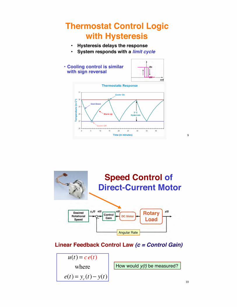
Thermostat Control Logic with Hysteresis
•! Hysteresis delays the response•! System responds with a limit cycle
•!Cooling control is similar with sign reversal
9
Speed Control of Direct-Current Motor
u(t) = ce(t)where
e(t) = yc(t)! y(t)
How would y(t) be measured?
Angular Rate
Linear Feedback Control Law (c = Control Gain)
10

Characteristics of the Model
•! Simplified Dynamic Model–! Rotary inertia, J, is the sum of motor and load inertias–! Internal damping neglected–! Output speed, y(t), rad/s, is an integral of the control
input, u(t)–! Motor control torque is proportional to u(t) –! Desired speed, yc(t), rad/s, is constant
11
1/J
Model of Dynamics and Speed Control
First-order LTI ordinary differential equation
y(t) = 1J
u(t)dt0
t
! = cJ
e(t)dt0
t
! = cJ
yc(t)" y(t)[ ]dt0
t
!
= " cJ
y(t)[ ]dt0
t
! + cJ
yc(t)[ ]dt0
t
!
dy(t)dt
=1Ju(t) = c
Je(t) = c
Jyc (t) ! y(t)[ ], y 0( ) given
Integral of the equation, with y(0) = 0
•!Positive integration of yc(t)•!Negative feedback of y(t) 12
c
Angular Rate
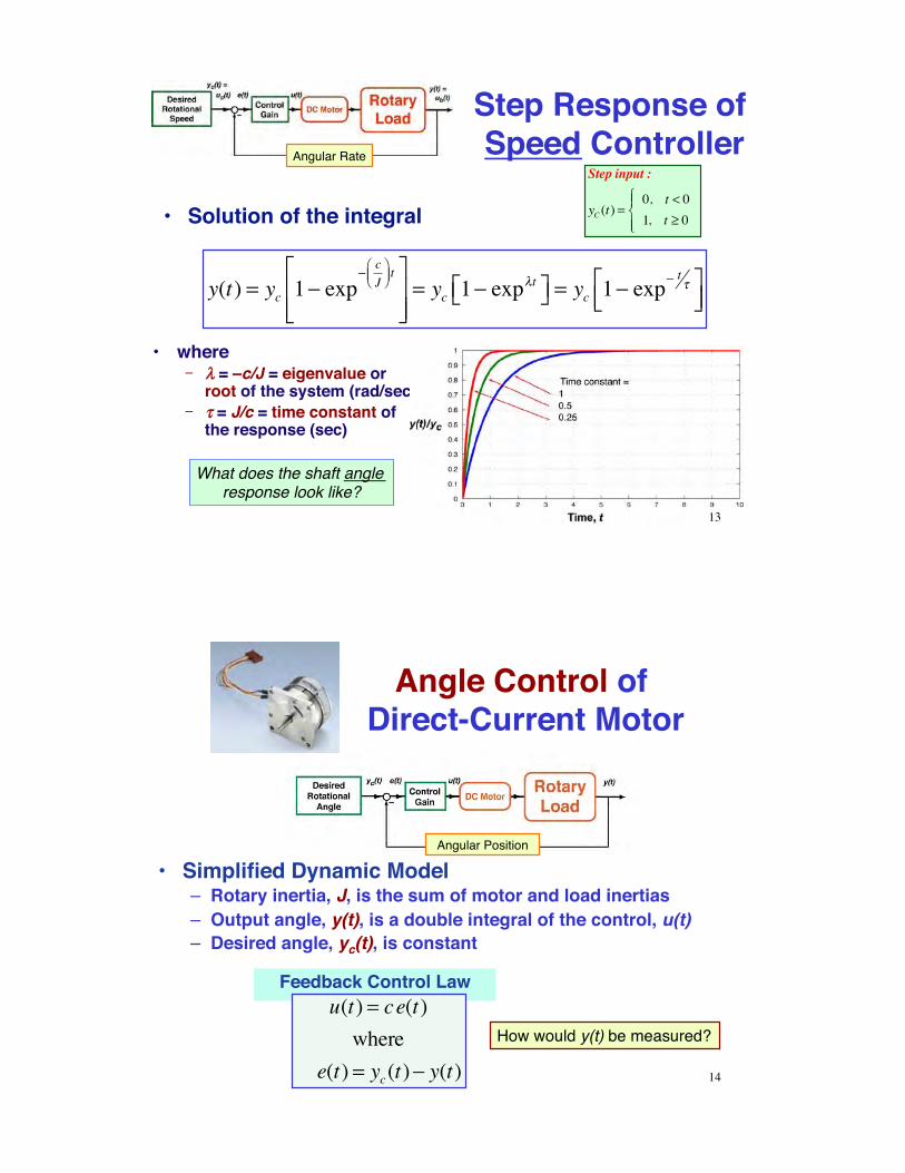
Step Response of Speed Controller
y(t) = yc 1! exp!
cJ
"#$
%&' t(
)**
+
,--= yc 1! exp
.t() +, = yc 1! exp! t /(
)*+,-
•! where! !! = –c/J = eigenvalue or
root of the system (rad/sec)! "" = J/c = time constant of
the response (sec)
Step input :
yC (t) =0, t < 01, t ! 0
"#$
%$•! Solution of the integral
What does the shaft angle response look like?
13
Angular Rate
Feedback Control Lawu(t) = ce(t)where
e(t) = yc(t)! y(t)
How would y(t) be measured?
Angular Position
•! Simplified Dynamic Model–! Rotary inertia, J, is the sum of motor and load inertias–! Output angle, y(t), is a double integral of the control, u(t)–! Desired angle, yc(t), is constant
Angle Control of Direct-Current Motor
14

Model of Dynamics and Angle Control
y(t) = cJ
yc ! y(t)[ ]0
t
" dt dt0
t
"
= ! cJ
y(t)[ ]0
t
" dt 20
t
" + cJ
yc[ ]0
t
" dt 20
t
"
2nd-order, linear, time-invariant ordinary differential equation
d 2y(t)dt 2
= !!y(t) = 1Ju t( ) = c
Je t( ) = c
Jyc ! y(t)[ ]
Output angle, y(t), as a function of time
15
Angular Position
Model of Dynamics and Angle Control•! Corresponding set of 1st-order equations, with
–! Angle: x1(t) = y(t)–! Angular rate: x2(t) = dy(t)/dt
!x1(t) = x2 (t)
!x2 (t) =u(t)J
= cJyc ! y(t)[ ] = c
Jyc ! x1(t)[ ]
16
Angular Position
State-Space Model of the DC Motor
Open-loop dynamic equation
!x1(t)!x2 (t)
!
"##
$
%&&= 0 1
0 0!
"#
$
%&
x1(t)x2 (t)
!
"##
$
%&&+ 0
1 / J!
"#
$
%&u(t)
Closed-loop dynamic equation
Feedback control law
u(t) = c yc (t) ! y1(t)[ ]= c yc (t) ! x1(t)[ ]
!x1(t)!x2 (t)
!
"##
$
%&&= 0 1
'c / J 0!
"#
$
%&
x1(t)x2 (t)
!
"##
$
%&&+ 0
c / J!
"#
$
%& yc
17
Step Response with Angle Feedback
% Step Response of Undamped Angle Control F1 = [0 1;-1 0]; G1 = [0;1]; F2 = [0 1;-0.5 0]; G2 = [0;0.5]; F3 = [0 1;-0.25 0]; G3 = [0;0.25]; Hx = [1 0;0 1]; Sys1 = ss(F1,G1,Hx,0); Sys2 = ss(F2,G2,Hx,0); Sys3 = ss(F3,G3,Hx,0); step(Sys1,Sys2,Sys3)
c/J = 1, 0.5, and 0.25
!x1(t)!x2 (t)
!
"##
$
%&&= 0 1
'c / J 0!
"#
$
%&
x1(t)x2 (t)
!
"##
$
%&&+ 0
c / J!
"#
$
%& yc
18

What Went Wrong?•! No damping!•! Solution: Add rate feedback in
the control law
Closed-loop dynamic equation
u(t) = c1 yc (t) ! y1(t)[ ]! c2y2 (t)
!x1(t)!x2 (t)
!
"##
$
%&&=
0 1'c1 / J 'c2 / J
!
"##
$
%&&
x1(t)x2 (t)
!
"##
$
%&&+
0c1 / J
!
"##
$
%&&yc
•! Control law with rate feedback
19
Alternative Implementations of Rate Feedback
One input, two outputs
u(t) = c1 yc (t) ! y1(t)[ ]! c2y2(t) = c1 yc (t) ! y1(t)[ ]! c2dy1(t)dt
One input, one output
20

c1 /J = 1 c2 /J = 0, 1.414, 2.828
% Step Response of Damped Angle Control F1 = [0 1;-1 0]; G1 = [0;1]; F1a = [0 1;-1 -1.414]; F1b = [0 1;-1 -2.828]; Hx = [1 0;0 1]; Sys1 = ss(F1,G1,Hx,0); Sys2 = ss(F1a,G1,Hx,0); Sys3 = ss(F1b,G1,Hx,0); step(Sys1,Sys2,Sys3)
Step Response with Angle and Rate Feedback
21
LTI Model with Feedback Control•! Command input, uc, has dimensions of u
˙ x (t) = F x(t) + Gu(t) + Lw(t)y(t) = Hxx(t) + Huu(t)u(t) = uc (t) !Cy(t)
22

LTI Control with Forward-Loop Gain
˙ x (t) = F x(t) + Gu(t) + Lw(t)y(t) = Hxx(t) + Huu(t)
u(t) = C yc (t) ! y(t)[ ]
With Cc = C, command input, yc, has dimensions of y23
Effect of Feedback Control on the LTI Model
!x(t) = Fx(t) +Gu(t) = Fx(t) +G uc (t) !Cy(t)[ ]= Fopen loop x(t) +G uc (t) !C Hxx(t)[ ]{ }
Feedback modifies the stability matrix of the closed-loop system
Convergence or divergenceEnvelope of transient response
= F !GCHx[ ]x(t)+Guc(t)! Fclosed loopx(t)+Guc(t)
24
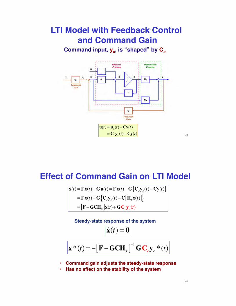
LTI Model with Feedback Control and Command Gain
Command input, yc, is shaped by Cc
u(t) = uc(t)!Cy(t)= Ccyc(t)!Cy(t) 25
Effect of Command Gain on LTI Model
!x(t) = Fx(t)+Gu(t) = Fx(t)+G Ccyc(t)!Cy(t){ }= Fx(t)+G Ccyc(t)!C Hxx(t)[ ]{ }= F !GCHx[ ]x(t)+GCcyc(t)
Steady-state response of the system
x * (t) = ! F !GCHx[ ]!1GCcyc * (t)
•! Command gain adjusts the steady-state response•! Has no effect on the stability of the system
!x(t) = 0
26
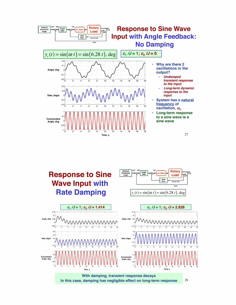
Response to Sine Wave Input with Angle Feedback:
No Dampingc1 /J = 1; c2 /J = 0yc (t) = sin ! t( ) = sin 6.28 t( ), deg
•! Why are there 2 oscillations in the output?
–! Undamped transient response to the input
–! Long-term dynamic response to the input
•! System has a natural frequency of oscillation, ##n
•! Long-term response to a sine wave is a sine wave
27
Response to Sine Wave Input with
Rate Dampingc1 /J = 1; c2 /J = 1.414 c1 /J = 1; c2 /J = 2.828
yc (t) = sin ! t( ) = sin 6.28 t( ), deg
With damping, transient response decaysIn this case, damping has negligible effect on long-term response 28

System Dynamics Produces Differences in Amplitude and
Phase Angle of Input and Output
Amplitude ratio and phase angle characterize the
system model
29
Amplitude Ratio (AR) =yOutput PeakyInput Peak
Phase Angle = 360tInput Peak ! tOutput Peak( )Period of Input
, deg
Effect of Input Frequency on Output Amplitude and
Phase Anglec1 /J = 1; c2 /J = 1.414
•! With low input frequency, input and output amplitudes are about the same
•! Output angle oscillation “lags” input by a few degrees
•! Rate oscillation leads angle
oscillation by ~90 deg
yc(t) = sin t / 6.28( ), deg
30

At Higher Frequency, Output Amplitude Decreases, Phase Angle Lag Increases
c1 /J = 1; c2 /J = 1.414yc(t) = sin t( ), deg
31
c1 /J = 1; c2 /J = 1.414
yc(t) = sin 6.28 t( ), deg At Even Higher Frequency, Amplitude Ratio Decreases
32
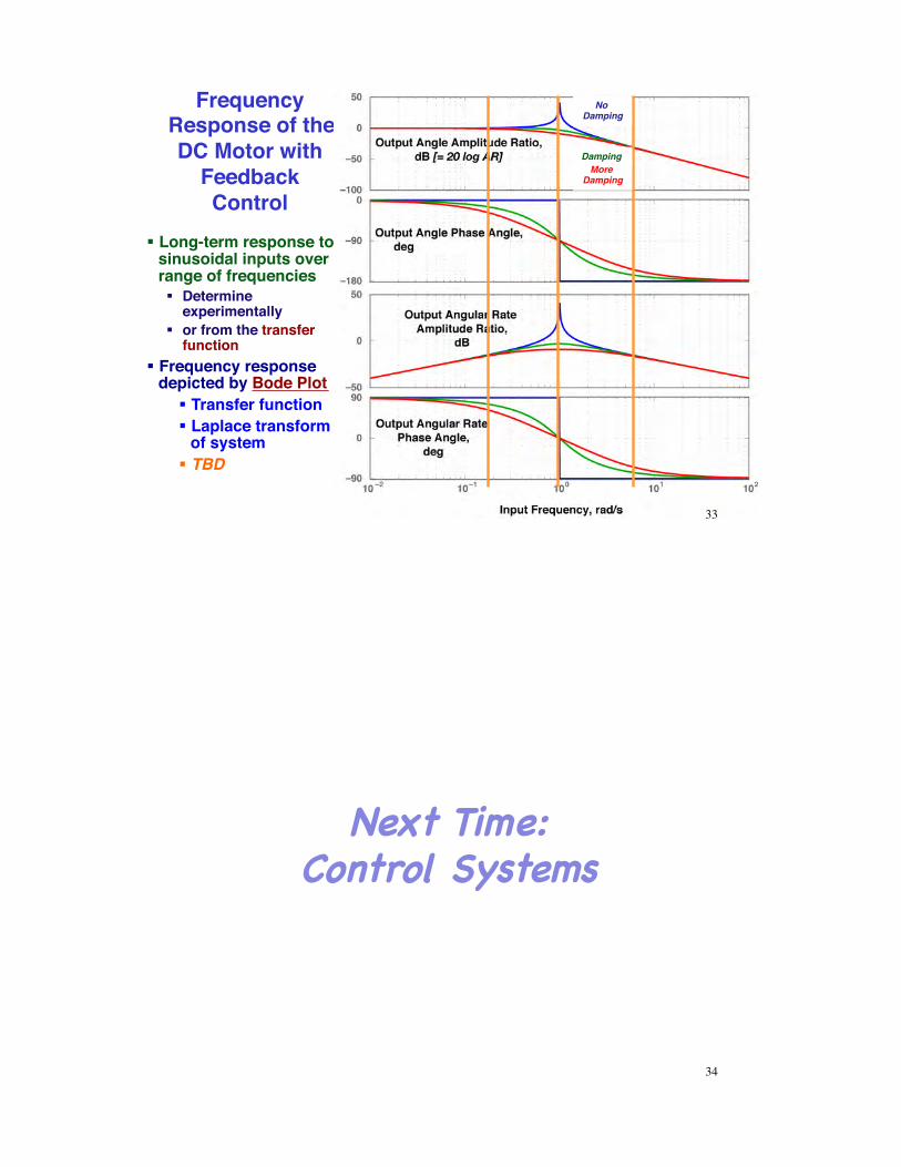
Frequency Response of the DC Motor with
Feedback Control
!!Long-term response to sinusoidal inputs over range of frequencies!! Determine
experimentally !! or from the transfer
function!!Frequency response
depicted by Bode Plot !!Transfer function!!Laplace transform
of system!!TBD
33
No Damping
More Damping
Damping
Next Time:!Control Systems!
34
Related Documents