Dynamic Computations in Ever-Changing Networks Idit Keidar Technion, Israel 1Idit Keidar, TADDS Sep 2011.

1

Dynamic Computations in Ever-Changing Networks

Dynamic Computations in Ever-Changing Networks

Idit KeidarTechnion, Israel

Idit Keidar, TADDS Sep 2011

2

TADDS: Theory of DynamicDistributed Systems

TADDS: Theory of DynamicDistributed Systems

(This Workshop)

?


3

What I Mean By “Dynamic”*What I Mean By “Dynamic”*

• A dynamic computation– Continuously adapts its output

to reflect input and environment changes

• Other names– Live, on-going, continuous, stabilizing

*In this talk Idit Keidar, TADDS Sep 2011

4

In This Talk: Three ExamplesIn This Talk: Three Examples

• Continuous (dynamic) weighted matching

• Live monitoring – (Dynamic) average aggregation)

• Peer sampling– Aka gossip-based membership


5

Ever-Changing Networks*Ever-Changing Networks*

• Where dynamic computations are interesting• Network (nodes, links) constantly changes• Computation inputs constantly change

– E.g., sensor reads• Examples:

– Ad-hoc, vehicular nets – mobility– Sensor nets – battery, weather – Social nets – people change friends, interests– Clouds spanning multiple data-centers – churn

*My name for “dynamic” networks Idit Keidar, TADDS Sep 2011

6

Continuous Weighted Matching

in Dynamic Networks

Continuous Weighted Matching

in Dynamic Networks

With Liat Atsmon Guz, Gil Zussman

Dynamic

Ever-Changing


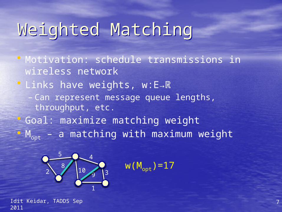
Weighted MatchingWeighted Matching

• Motivation: schedule transmissions in wireless network

• Links have weights, w:E→ℝ– Can represent message queue lengths,

throughput, etc.• Goal: maximize matching weight• Mopt – a matching with maximum weight

8

5

2 9

4

10 3

1

w(Mopt)=177


8

ModelModel

• Network is ever-changing, or dynamic– Also called time-varying graph, dynamic

communication network, evolving graph– Et,Vt are time-varying sets, wt is a time-

varying function • Asynchronous communication• No message loss unless links/node

crash– Perfect failure detection


9

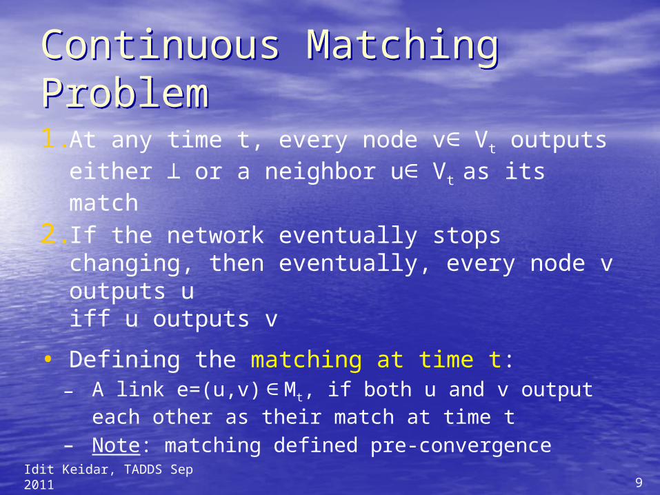
Continuous Matching ProblemContinuous Matching Problem1.At any time t, every node v∈ Vt outputs

either ⊥ or a neighbor u∈ Vt as its match

2. If the network eventually stops changing, then eventually, every node v outputs u iff u outputs v

• Defining the matching at time t:– A link e=(u,v) ∈ Mt, if both u and v output

each other as their match at time t– Note: matching defined pre-convergence


10

Classical Approach to MatchingClassical Approach to Matching• One-shot (static) algorithms• Run periodically

– Each time over static input• Bound convergence time

– Best known in asynchronous networks is O(|V|)• Bound approximation ratio at the end

– Typically 2• Don’t use the matching while algorithm is

running – “Control phase”


11

Self-Stabilizing ApproachSelf-Stabilizing Approach

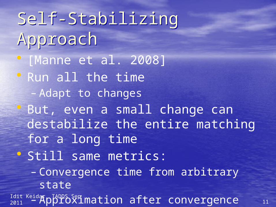
• [Manne et al. 2008]• Run all the time

– Adapt to changes• But, even a small change can

destabilize the entire matching for a long time

• Still same metrics:– Convergence time from arbitrary state– Approximation after convergence


12

Our Approach: Maximize Matching “All the Time”Our Approach: Maximize Matching “All the Time”• Run constantly

– Like self-stabilizing• Do not wait for convergence

– It might never happen in a dynamic network!• Strive for stability

– Keep current matching edges in the matching as much as possible

• Bound approximation throughout the run– Local steps can take us back to the

approximation quickly after a local change


13

Continuous Matching StrawmanContinuous Matching Strawman• Asynchronous matching using

Hoepman’s (1-shot) Algorithm– Always pick “locally” heaviest link for

the matching– Convergence in O(|V|) time from scratch

• Use same rule dynamically: if new locally heaviest link becomes available, grab it and drop conflicting links


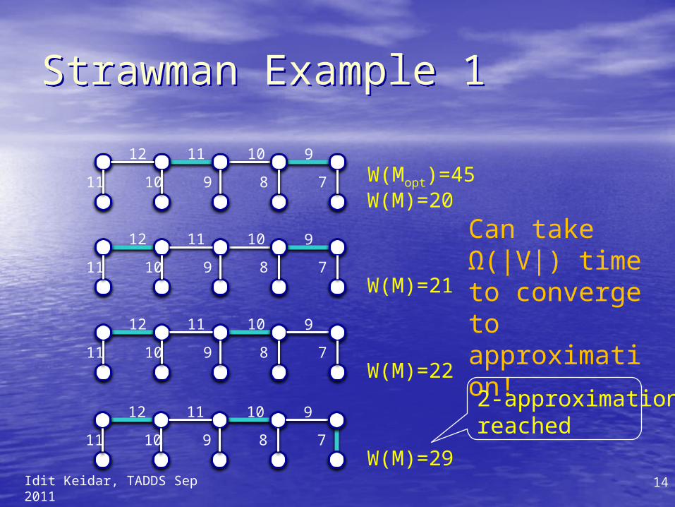
Strawman Example 1Strawman Example 1

11 10 9

14

10 9

12

11 78 W(Mopt)=45W(M)=20

11 10 9

10 9

12

11 78W(M)=21

11 10 9

10 9

12

11 78W(M)=22

11 10 9

10 9

12

11 78W(M)=29

Can take Ω(|V|) time to converge to approximation!

2-approximationreached


15

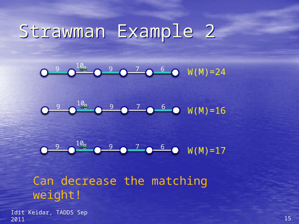
Strawman Example 2Strawman Example 2


9 7 68109

9 7 68109

W(M)=24

W(M)=16

9 7 68109 W(M)=17

Can decrease the matching weight!

16

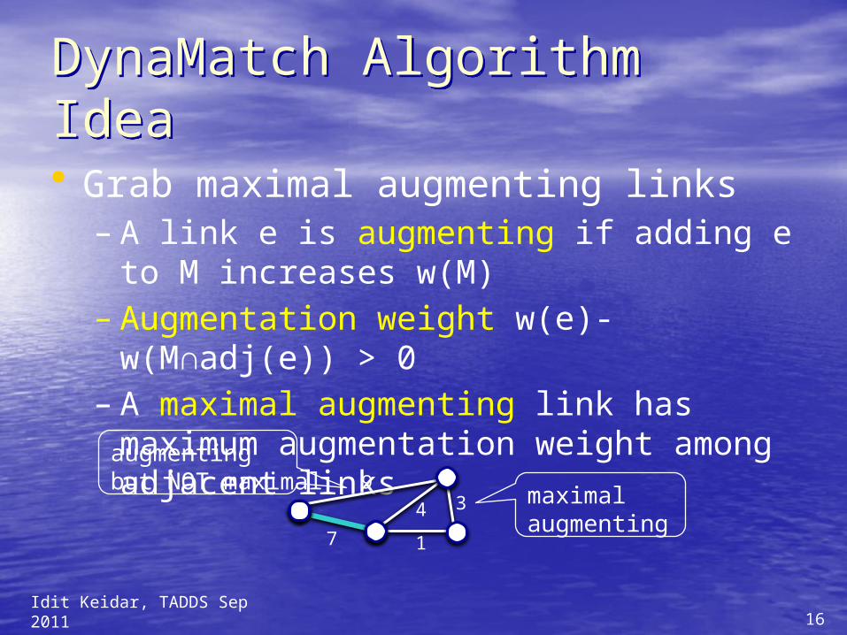
DynaMatch Algorithm IdeaDynaMatch Algorithm Idea

• Grab maximal augmenting links – A link e is augmenting if adding e to M

increases w(M)– Augmentation weight w(e)-w(M∩adj(e))

> 0– A maximal augmenting link has

maximum augmentation weight among adjacent links


4

9

7

3

1

augmenting but NOT maximal

maximalaugmenting

17

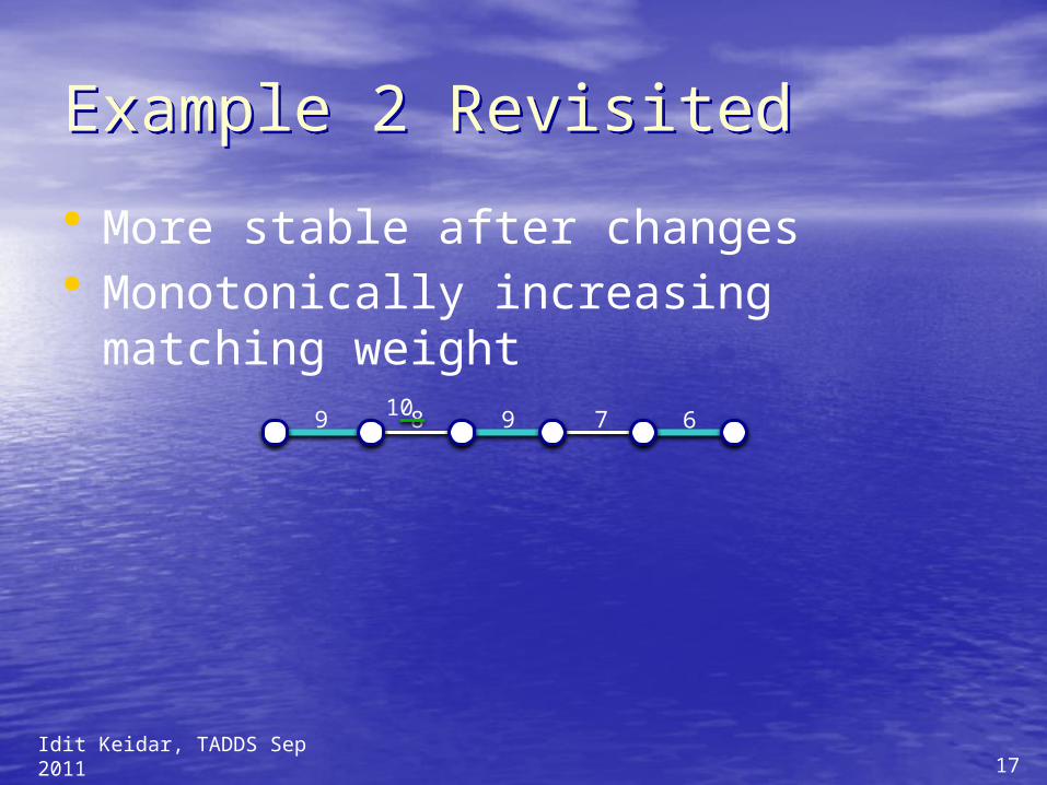
• More stable after changes• Monotonically increasing matching

weight

Example 2 RevisitedExample 2 Revisited

9 7 68109


18

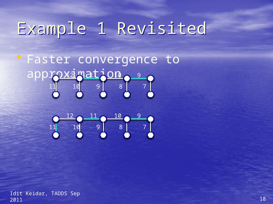
Example 1 RevisitedExample 1 Revisited

• Faster convergence to approximation11 10 9

10 9

12

11 78

11 10 9

10 9

12

11 78


19

General ResultGeneral Result

• After a local change– Link/node added, removed, weight

change• Convergence to approximation within

constant number of steps – Even before algorithm is quiescent

(stable)– Assuming it has stabilized before the

change


20

LiMoSense – Live Monitoring in Dynamic Sensor NetworksLiMoSense – Live Monitoring in Dynamic Sensor Networks

With Ittay Eyal, Raphi RomALGOSENSORS'11

Dynamic

Ever-Changing


21

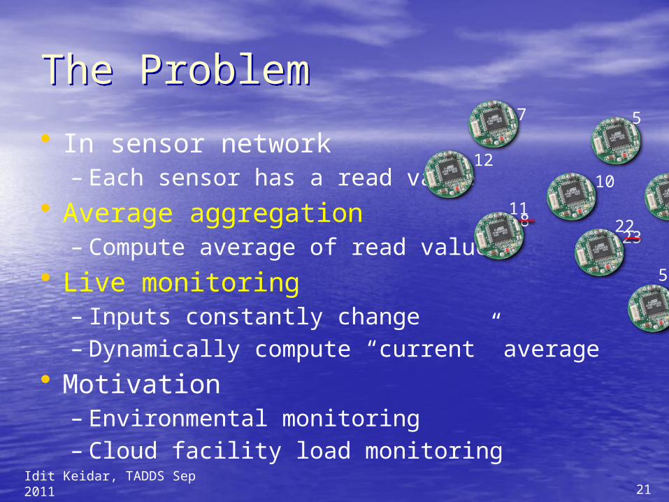
The ProblemThe Problem

• In sensor network– Each sensor has a read value

• Average aggregation – Compute average of read values

• Live monitoring– Inputs constantly change– Dynamically compute “current” average

• Motivation– Environmental monitoring– Cloud facility load monitoring


7

12

823

5

5

10

1122

22

RequirementsRequirements

• Robustness– Message loss– Link failure/recovery – battery decay,

weather– Node crash

• Limited bandwidth (battery), memory in nodes (motes)

• No centralized server– Challenge: cannot collect the values – Employ in-network aggregation


23

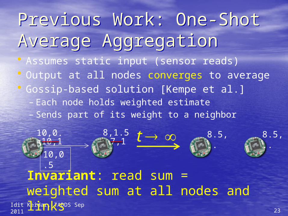
Previous Work: One-Shot Average AggregationPrevious Work: One-Shot Average Aggregation• Assumes static input (sensor reads)• Output at all nodes converges to average• Gossip-based solution [Kempe et al.]

– Each node holds weighted estimate– Sends part of its weight to a neighbor


10,1 7,1

10,0.5

10,0.5

8,1.5 8.5, ..

t 8.5, ..

Invariant: read sum = weighted sum at all nodes and links

24

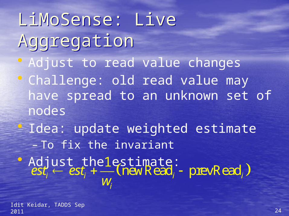
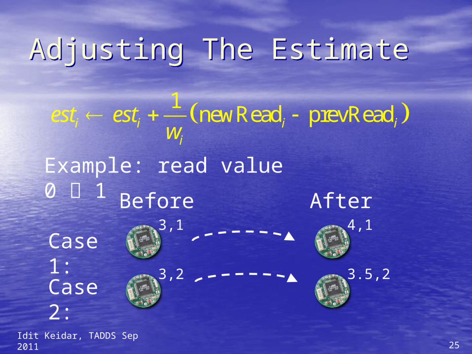
LiMoSense: Live AggregationLiMoSense: Live Aggregation• Adjust to read value changes• Challenge: old read value may have

spread to an unknown set of nodes• Idea: update weighted estimate

– To fix the invariant• Adjust the estimate:


1newRead prevReadi i i i

i

est estw

25

Adjusting The Estimate Adjusting The Estimate


Case 1:

Case 2:

Example: read value 0 1 Before After

1newRead prevReadi i i i

i

est estw

3,1

3,2 3.5,2

4,1

26

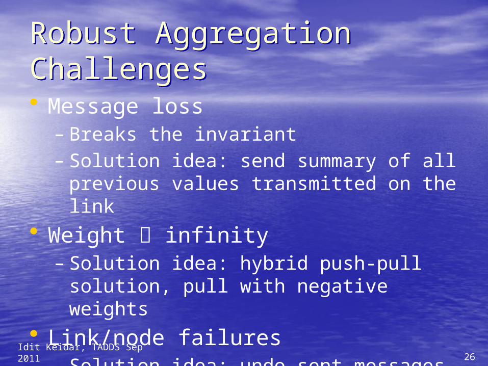
Robust Aggregation ChallengesRobust Aggregation Challenges• Message loss

– Breaks the invariant – Solution idea: send summary of all

previous values transmitted on the link• Weight infinity

– Solution idea: hybrid push-pull solution, pull with negative weights

• Link/node failures– Solution idea: undo sent messages


27

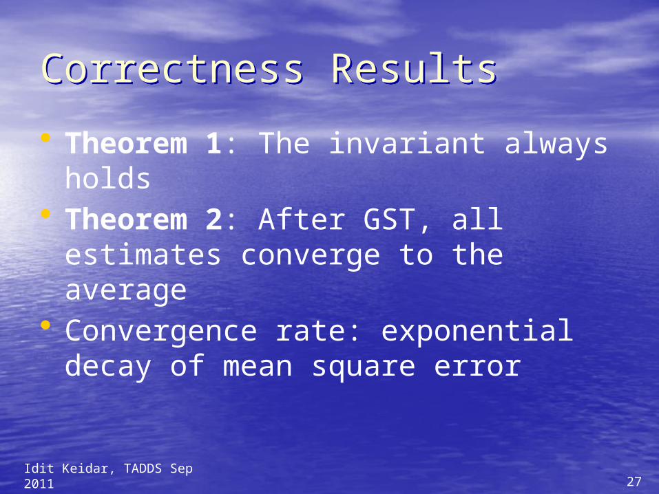
Correctness ResultsCorrectness Results

• Theorem 1: The invariant always holds

• Theorem 2: After GST, all estimates converge to the average

• Convergence rate: exponential decay of mean square error


28

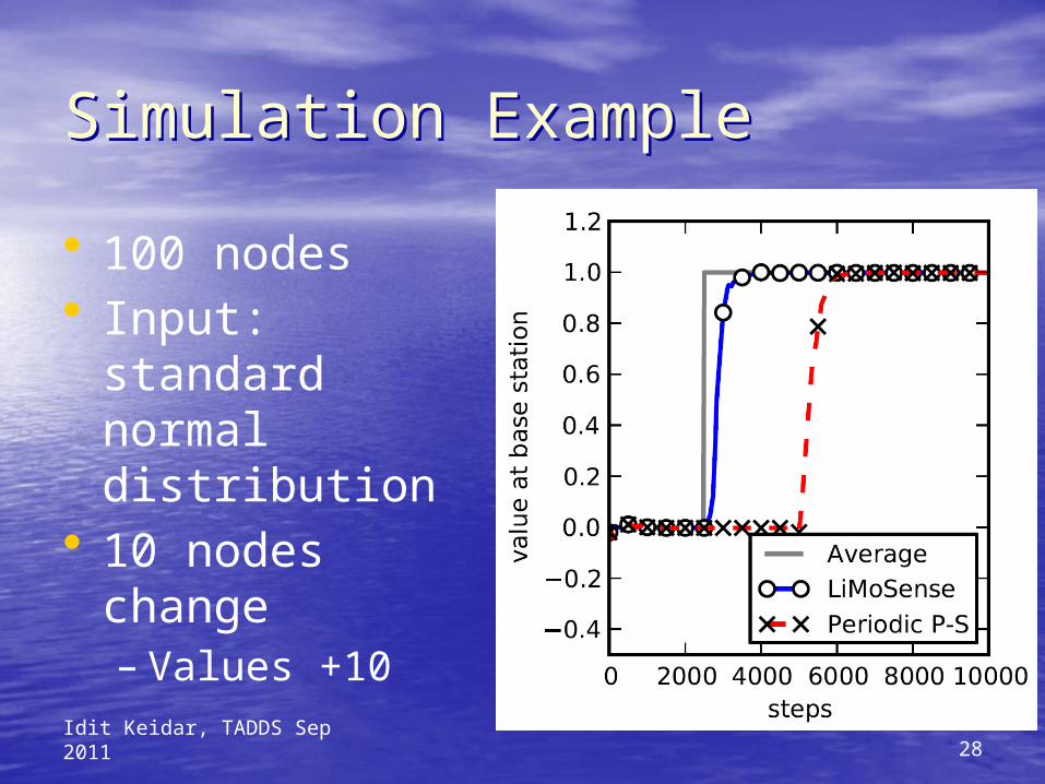
Simulation ExampleSimulation Example

• 100 nodes • Input: standard

normal distribution

• 10 nodes change – Values +10


29

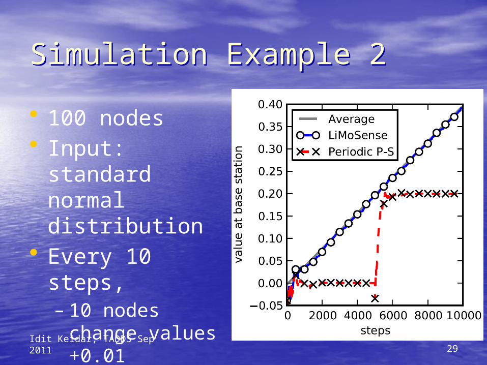
Simulation Example 2Simulation Example 2

• 100 nodes • Input: standard

normal distribution

• Every 10 steps, – 10 nodes change

values +0.01


30

SummarySummary

• LiMoSense – Live Average Monitoring– Aggregate dynamic data reads

• Fault tolerant– Message loss, link failure, node crash

• Correctness in dynamic asynchronous settings

• Exponential convergence after GST• Quick reaction to dynamic behavior


31

Correctness of Gossip-Based Membership under Message Loss

Correctness of Gossip-Based Membership under Message Loss

With Maxim GurevichPODC'09; SICOMP 2010

Dynamic


32

The SettingThe Setting

• Many nodes – n– 10,000s, 100,000s, 1,000,000s, …

• Come and go– Churn (=ever-changing input)

• Fully connected network topology– Like the Internet

• Every joining node knows some others– (Initial) Connectivity


33

Membership or Peer SamplingMembership or Peer Sampling• Each node needs to know some live

nodes• Has a view

– Set of node ids– Supplied to the application– Constantly refreshed (= dynamic

output)• Typical size – log n


34

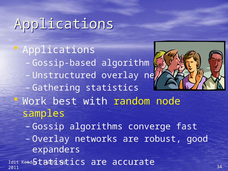
ApplicationsApplications

• Applications– Gossip-based algorithm– Unstructured overlay networks– Gathering statistics

• Work best with random node samples– Gossip algorithms converge fast– Overlay networks are robust, good

expanders– Statistics are accurate


35

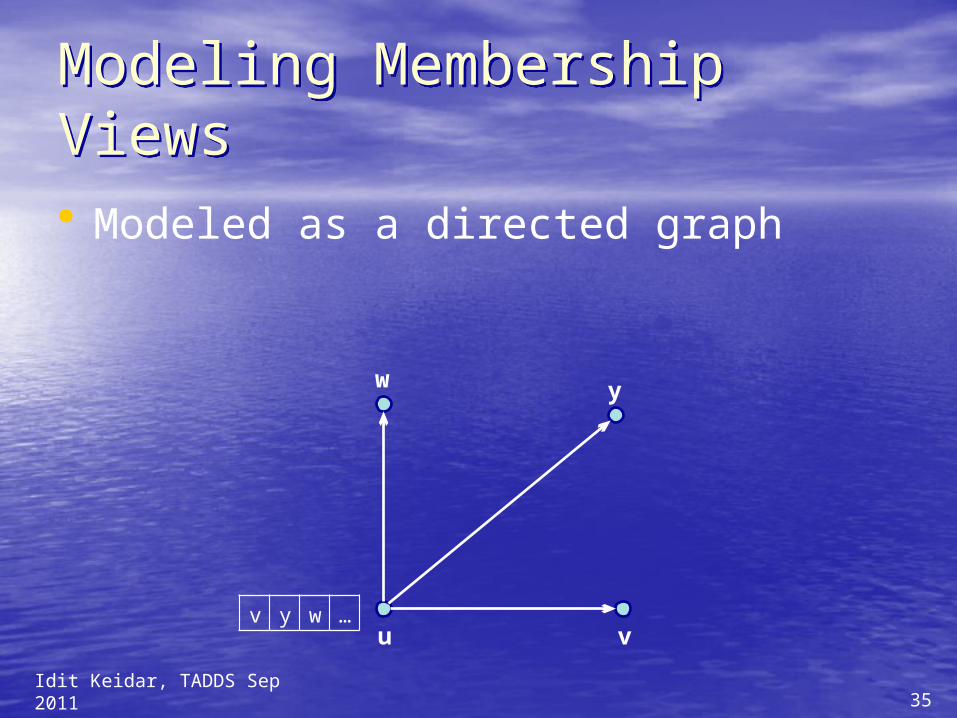
Modeling Membership ViewsModeling Membership Views

• Modeled as a directed graph

u v

w

v y w …

y


36

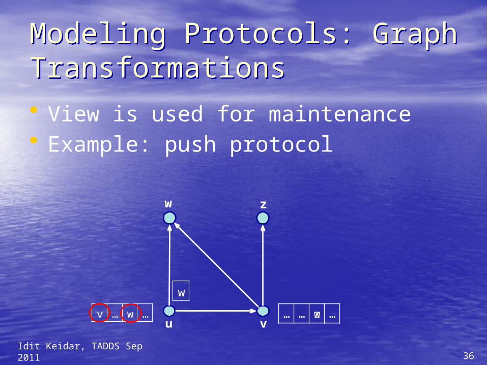
Modeling Protocols: Graph TransformationsModeling Protocols: Graph Transformations• View is used for maintenance• Example: push protocol

… … w …… … z …u v

w

v … w …

w

z


37

Desirable Properties?Desirable Properties?

• Randomness– View should include random samples

• Holy grail for samples: IID– Each sample uniformly distributed– Each sample independent of other

samples• Avoid spatial dependencies among view

entries• Avoid correlations between nodes

– Good load balance among nodesIdit Keidar, TADDS Sep 2011

38

What About Churn?What About Churn?

• Views should constantly evolve– Remove failed nodes, add joining ones

• Views should evolve to IID from any state

• Minimize temporal dependencies– Dependence on the past should decay

quickly – Useful for application requiring fresh

samples


39

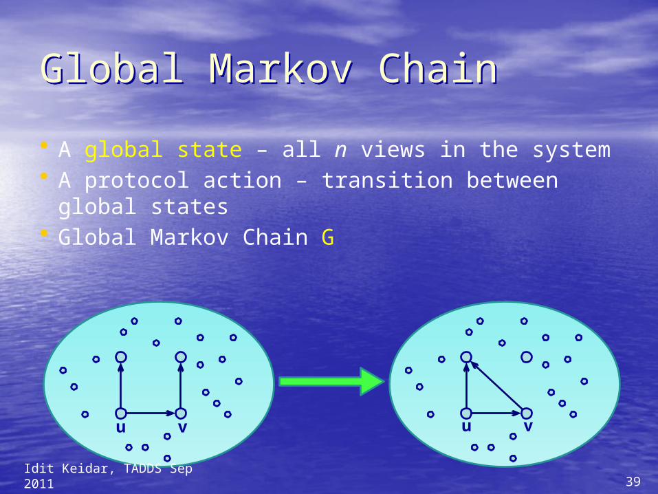
Global Markov ChainGlobal Markov Chain

• A global state – all n views in the system• A protocol action – transition between

global states• Global Markov Chain G

u v u v


40

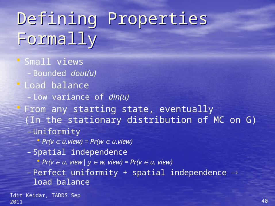
Defining Properties FormallyDefining Properties Formally

• Small views– Bounded dout(u)

• Load balance– Low variance of din(u)

• From any starting state, eventually(In the stationary distribution of MC on G)– Uniformity

• Pr(v u.view) = Pr(w u.view)

– Spatial independence• Pr(v u. view| y w. view) = Pr(v u. view)

– Perfect uniformity + spatial independence load balance


41

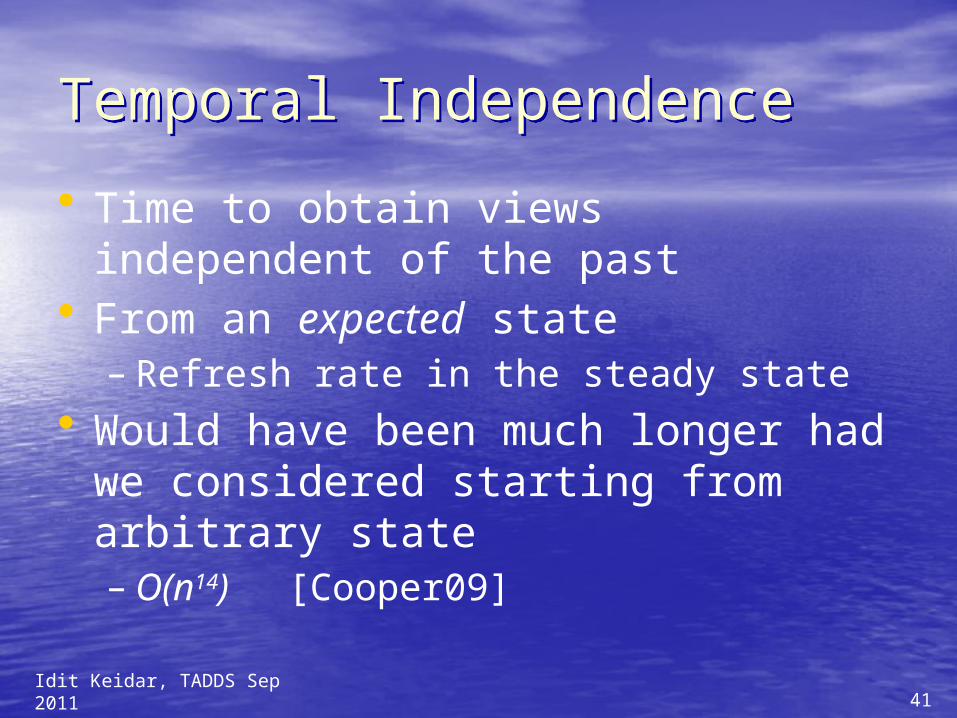
Temporal IndependenceTemporal Independence

• Time to obtain views independent of the past

• From an expected state– Refresh rate in the steady state

• Would have been much longer had we considered starting from arbitrary state– O(n14) [Cooper09]


42

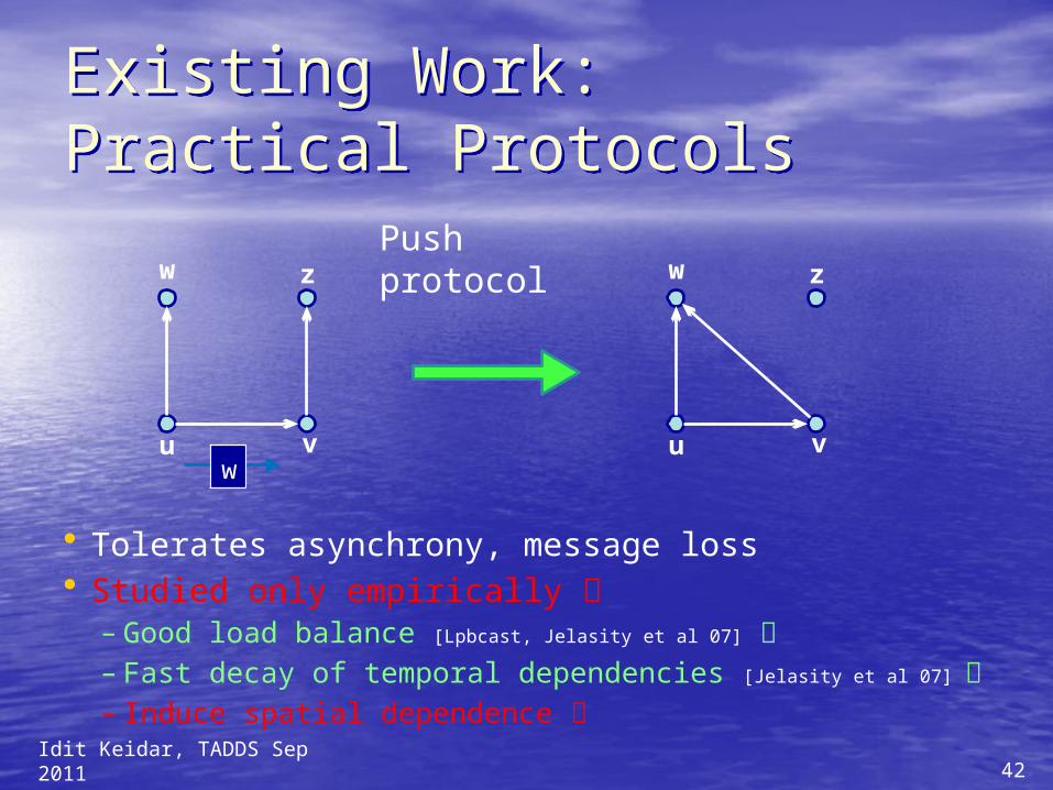
Existing Work: Practical ProtocolsExisting Work: Practical Protocols

• Tolerates asynchrony, message loss• Studied only empirically

– Good load balance [Lpbcast, Jelasity et al 07] – Fast decay of temporal dependencies [Jelasity et al 07] – Induce spatial dependence

Push protocol

u v

w

u v

w

w

z z


43

v … z …

Existing Work: AnalysisExisting Work: Analysis

• Analyzed theoretically [Allavena et al 05, Mahlmann et al 06]

– Uniformity, load balance, spatial independence – Weak bounds (worst case) on temporal independence

• Unrealistic assumptions – hard to implement – Atomic actions with bi-directional communication– No message loss

… … z …… … w …u v

w

v … w …

w

zShuffle protocol

z

*


44

Our Contribution : Bridge This GapOur Contribution : Bridge This Gap

• A practical protocol– Tolerates message loss, churn, failures– No complex bookkeeping for atomic

actions• Formally prove the desirable

properties– Including under message loss


45

… …

Send & Forget MembershipSend & Forget Membership• The best of push and shuffle

u v

w

v … w … u w

u w

• Perfect randomness without loss

Some view entries may be empty


46

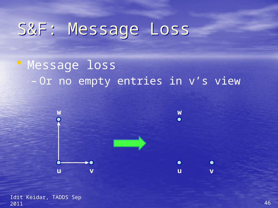
S&F: Message LossS&F: Message Loss

• Message loss– Or no empty entries in v’s view

u v

w

u v

w


47

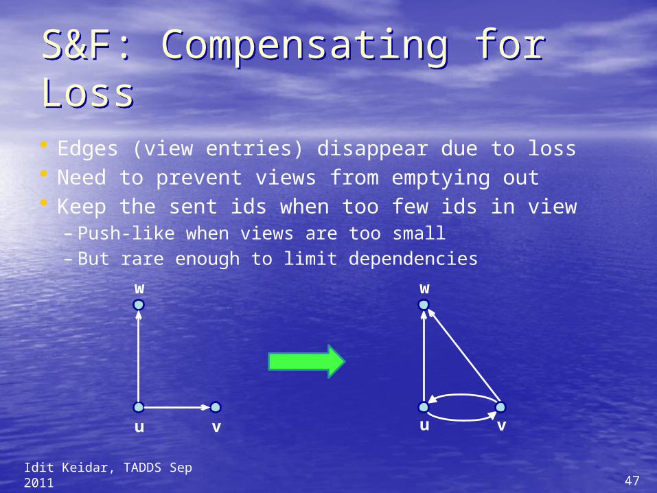
S&F: Compensating for LossS&F: Compensating for Loss

• Edges (view entries) disappear due to loss• Need to prevent views from emptying out• Keep the sent ids when too few ids in view

– Push-like when views are too small– But rare enough to limit dependencies

u v

w

u v

w


48

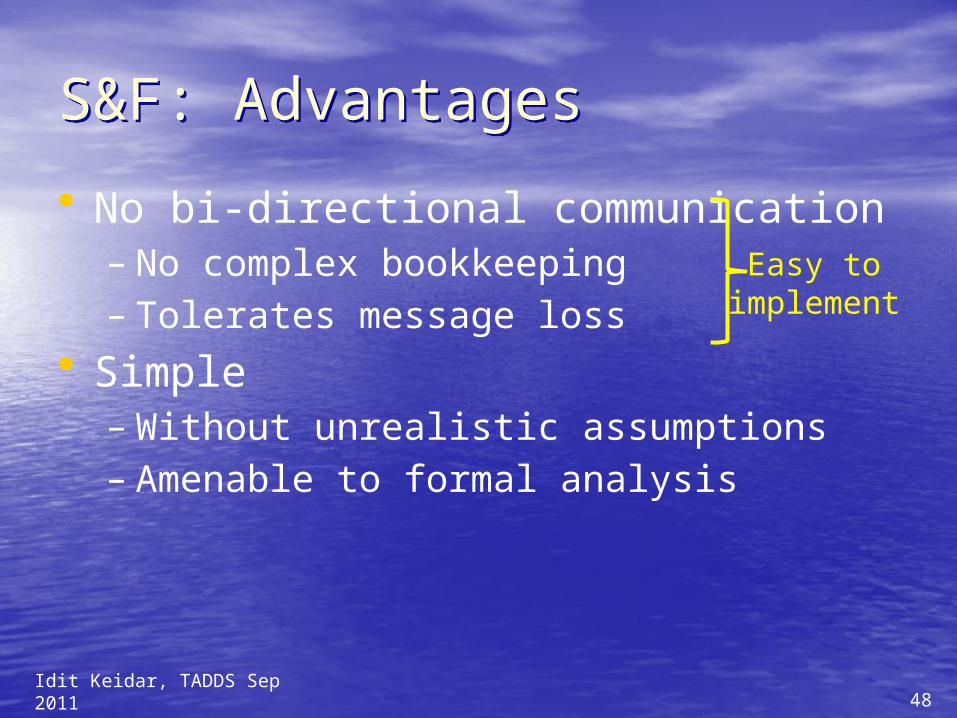
S&F: AdvantagesS&F: Advantages

• No bi-directional communication– No complex bookkeeping– Tolerates message loss

• Simple– Without unrealistic assumptions– Amenable to formal analysis

Easy to implement


49

• Degree distribution (load balance)• Stationary distribution of MC on

global graph G– Uniformity– Spatial Independence– Temporal Independence

• Hold even under (reasonable) message loss!

Key Contribution: AnalysisKey Contribution: Analysis


50

ConclusionsConclusions

• Ever-changing networks are here to stay

• In these, need to solve dynamic versions of network problems

• We discussed three examples – Matching– Monitoring– Peer sampling

• Many more have yet to be studiedIdit Keidar, TADDS Sep 2011

51

Thanks!Thanks!

• Liat Atsmon Guz, Gil Zussman• Ittay Eyal, Raphi Rom• Maxim Gurevich


Dynamic Computations in Ever-Changing Networks Idit Keidar Technion, Israel 1Idit Keidar, TADDS Sep 2011.

Documents

dynamic networks

time t

dynamic computations

dynamic communication

continuous weighted

weighted matching motivation

continuous matching

matching weight goal