Dynamic binaural sound localization based on variations of interaural time delays and system rotations Claude Baumann, 1,a) Chris Rogers, 2 and Francis Massen 1 1 Lyc ee Classique Diekirch, Computarium, 32 Avenue de la Gare, Diekirch 9233, Luxembourg 2 Tufts University, School of Engineering, 200 College Avenue, Medford, Massachusetts 02155, USA (Received 7 February 2015; revised 16 June 2015; accepted 22 June 2015; published online 6 August 2015) This work develops the mathematical model for a steerable binaural system that determines the in- stantaneous direction of a sound source in space. The model combines system angular speed and interaural time delays (ITDs) in a differential equation, which allows monitoring the change of source position in the binaural reference frame and therefore resolves the confusion about azimuth and elevation. The work includes the analysis of error propagation and presents results from a real- time application that was performed on a digital signal processing device. Theory and experiments demonstrate that the azimuthal angle to the sound source is accurately yielded in the case of hori- zontal rotations, whereas the elevation angle is estimated with large uncertainty. This paper also proves the equivalence of the ITD derivative and the Doppler shift appearing between the binau- rally captured audio signals. The equation of this Doppler shift is applicable for any kind of motion. It shows that weak binaural pitch differences may represent an additional cue in localization of sound. Finally, the paper develops practical applications from this relationship, such as the synthe- sizing of binaural images of pure and complex tones emitted by a moving source, and the genera- tion of multiple frequency images for binaural beat experiments. V C 2015 Acoustical Society of America.[http://dx.doi.org/10.1121/1.4923448] [ICB] Pages: 635–650 I. INTRODUCTION One particularity of the auditory system in mammals is its physical proximity with the vestibular system, responsible for most of the animal balance and spatial orientation capaci- ties. The interconnection of both different sensory systems suggests that motion somehow contributes to complex forms of analysis of the auditory scene and more particularly of sound localization. In this paper, the authors want to give evidence that the dynamics of head rotations play an impor- tant role in three-dimensional (3D) sound localization. The work starts from a reduced binaural system capable of sens- ing interaural time delays (ITDs) and angular velocity and uses a differential equation to describe the involved dynam- ics, which forms a special view on ITDs by considering their variability over time. It is shown that the knowledge of three quantities, the instantaneous ITD, its first derivative with respect to time and the rotation speed of the binaural system unambiguously and robustly yields the azimuth in the case of a horizontal rotation, thus solving the back/front confu- sion. Additionally and much more unintuitively, it is demon- strated that theoretically the magnitude of the elevation is also yielded. The work includes the analysis of error propa- gation and proves that the elevation can only be validly esti- mated if the sound source is not located in the horizontal or the median plane. Furthermore, the paper presents results from a physi- cal experiment of the model using a high-speed digital sig- nal processing device. Finally, the authors demonstrate that one can determine the frequency modulation applied to the original acoustic signal because of the effect of head rotation. This might be considered as an additional cue in sound localization, expressing itself as a Doppler shift between the left and right signals. This binaural Doppler shift is proven to be mathematically equal to the ITD derivative. II. ROTATIONS AND SOUND LOCALIZATION A. Fundamentals For an immobile binaural system, the knowledge of interaural time delays (ITDs) cannot solve the localiza- tion problem better than yielding a lateral surface of all possible locations of the sound source for a specific delay. This surface represents the sheet of a hyperboloid of confusion, which is generated by revolving one branch of the hyperbola that can be constructed for a certain value of the ITD upon two foci formed by the acoustic receivers. 1 Asymptotically, the hyperbolic sheet changes to a conical surface. The confusion in spatial localization of sound therefore only disappears if other cues are available. In their mathematical and experimental study, Kneip and Baumann 2 have analyzed and proven the utility of delib- erate rotations of a binaural system for the determination of the direction in space of a static sound source. The described active method is based on the measurements of ITDs before and after a single determined rotation of the interaural base- line about the z or y axis. The equations show that the angu- lar component of the sound vector is unambiguously a) Electronic mail: [email protected] J. Acoust. Soc. Am. 138 (2), August 2015 V C 2015 Acoustical Society of America 635 0001-4966/2015/138(2)/635/16/$30.00

Welcome message from author
This document is posted to help you gain knowledge. Please leave a comment to let me know what you think about it! Share it to your friends and learn new things together.
Transcript
Dynamic binaural sound localization based on variationsof interaural time delays and system rotations
Claude Baumann,1,a) Chris Rogers,2 and Francis Massen1
1Lyc�ee Classique Diekirch, Computarium, 32 Avenue de la Gare, Diekirch 9233, Luxembourg2Tufts University, School of Engineering, 200 College Avenue, Medford, Massachusetts 02155, USA
(Received 7 February 2015; revised 16 June 2015; accepted 22 June 2015; published online 6August 2015)
This work develops the mathematical model for a steerable binaural system that determines the in-
stantaneous direction of a sound source in space. The model combines system angular speed and
interaural time delays (ITDs) in a differential equation, which allows monitoring the change of
source position in the binaural reference frame and therefore resolves the confusion about azimuth
and elevation. The work includes the analysis of error propagation and presents results from a real-
time application that was performed on a digital signal processing device. Theory and experiments
demonstrate that the azimuthal angle to the sound source is accurately yielded in the case of hori-
zontal rotations, whereas the elevation angle is estimated with large uncertainty. This paper also
proves the equivalence of the ITD derivative and the Doppler shift appearing between the binau-
rally captured audio signals. The equation of this Doppler shift is applicable for any kind of motion.
It shows that weak binaural pitch differences may represent an additional cue in localization of
sound. Finally, the paper develops practical applications from this relationship, such as the synthe-
sizing of binaural images of pure and complex tones emitted by a moving source, and the genera-
tion of multiple frequency images for binaural beat experiments.VC 2015 Acoustical Society of America. [http://dx.doi.org/10.1121/1.4923448]
[ICB] Pages: 635–650
I. INTRODUCTION
One particularity of the auditory system in mammals is
its physical proximity with the vestibular system, responsible
for most of the animal balance and spatial orientation capaci-
ties. The interconnection of both different sensory systems
suggests that motion somehow contributes to complex forms
of analysis of the auditory scene and more particularly of
sound localization. In this paper, the authors want to give
evidence that the dynamics of head rotations play an impor-
tant role in three-dimensional (3D) sound localization. The
work starts from a reduced binaural system capable of sens-
ing interaural time delays (ITDs) and angular velocity and
uses a differential equation to describe the involved dynam-
ics, which forms a special view on ITDs by considering their
variability over time. It is shown that the knowledge of three
quantities, the instantaneous ITD, its first derivative with
respect to time and the rotation speed of the binaural system
unambiguously and robustly yields the azimuth in the case
of a horizontal rotation, thus solving the back/front confu-
sion. Additionally and much more unintuitively, it is demon-
strated that theoretically the magnitude of the elevation is
also yielded. The work includes the analysis of error propa-
gation and proves that the elevation can only be validly esti-
mated if the sound source is not located in the horizontal or
the median plane.
Furthermore, the paper presents results from a physi-
cal experiment of the model using a high-speed digital sig-
nal processing device. Finally, the authors demonstrate
that one can determine the frequency modulation applied
to the original acoustic signal because of the effect of head
rotation. This might be considered as an additional cue in
sound localization, expressing itself as a Doppler shift
between the left and right signals. This binaural Doppler
shift is proven to be mathematically equal to the ITD
derivative.
II. ROTATIONS AND SOUND LOCALIZATION
A. Fundamentals
For an immobile binaural system, the knowledge of
interaural time delays (ITDs) cannot solve the localiza-
tion problem better than yielding a lateral surface of all
possible locations of the sound source for a specific
delay. This surface represents the sheet of a hyperboloid
of confusion, which is generated by revolving one branch
of the hyperbola that can be constructed for a certain
value of the ITD upon two foci formed by the acoustic
receivers.1 Asymptotically, the hyperbolic sheet changes
to a conical surface. The confusion in spatial localization
of sound therefore only disappears if other cues are
available.
In their mathematical and experimental study, Kneip
and Baumann2 have analyzed and proven the utility of delib-
erate rotations of a binaural system for the determination of
the direction in space of a static sound source. The described
active method is based on the measurements of ITDs before
and after a single determined rotation of the interaural base-
line about the z or y axis. The equations show that the angu-
lar component of the sound vector is unambiguouslya)Electronic mail: [email protected]
J. Acoust. Soc. Am. 138 (2), August 2015 VC 2015 Acoustical Society of America 6350001-4966/2015/138(2)/635/16/$30.00
determined in the plane of rotation, whereas the orthogonal
component appears in two symmetric instances. If the inter-
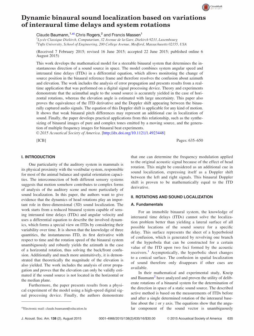
aural axis is rotated about the z axis, as indicated on Fig. 1,
the azimuth b is exactly yielded and the elevation w is found
with ambiguity, which means that the magnitude of the ele-
vation angle is known, but its sign is not. (Note that unlike
the cited paper, this text uses the symbol w for the elevation.
See Nomenclature.)
The present work starts from this viewpoint and deduces
further equations from the properties of the cone of confu-
sion. The following mathematical development proves that
the combination of continuous measurements and differen-
tiation of ITDs, and the measurements of the rotation speed
in a given plane determines the angular component of the
sound vector in that particular plane. Consequently, the mag-
nitude of the second orthogonal component also is deter-
mined, whereas its sign is not. The disambiguation of this
persistent uncertainty consists of clarifying whether the
sound source is located in the upper/lower, or the frontal/
backward hemispheres—depending on the rotation plane.
This requires little additional information that can be easily
obtained by complementary means, especially through a sin-
gle subsequent orthogonal rotation.
The mathematical description restricts the analysis to a
simple binaural sensor made of two omnidirectional micro-
phones in the free field, augmented with a sensor for meas-
uring angular velocity. Neither pinnae, nor head, nor torso
are involved. Therefore, no spectral or level differences are
considered. It is also assumed that the sound source, a single
immobile spot in space, is located in the far field. According
to Kneip and Baumann,2 deviations between the asymptotic
cone of confusion and the correct hyperbolic surface are less
than 1� for sound distances greater than 4k, and less than
0.1� for distances greater than 12k, where 2k is the micro-
phone spacing. Furthermore, the binaural system rotates
about the z axis, while the speed of the microphone
movements is very slow in comparison to the speed of
sound. It must be underlined that the orthogonal system of
coordinates ðO; x; y; zÞ is always referenced to the binaural
system using the interaural baseline as x axis. This must not
be confused with the “world” reference frame. Because the
coordinate system may be arbitrarily fixed in the median
plane (O, y, z), it is obvious that the present study in fact
covers any case of rotation of the binaural system, except the
one about the x axis. It should be noted that the choice of
this head referencing is consistent with the findings of
Altmann et al.,3 who concluded from their neurophysiologi-
cal study that humans process spatial changes of sound
source position in a head-related coordinate system.
This work is based on the insight that has been gained
through the research about natural sound localization in
combination with head rotations by van Soest,4 who stated
that through head movements, according to the phase theory,
the sound direction is given by the intersectional line of suc-
cessive cones of confusion. The approach of van Soest4 has
been verified by Reid and Milios5 using an approximation
method running on a digital signal processing device.
Wallach6 showed that head rotations provide essential infor-
mation about the azimuth and the elevation of the sound
source. His hypotheses have been testified by Perret and
Noble7 and Wightman and Kistler,8 for instance. Thurlow
et al.9 observed three types of head rotations about each of
the main axis that contribute to the localization of a sound
source in space. Hill et al.10 developed a simulation model
in order to show that back/front ambiguity may be resolved
through ITD variations arising from head rotation.
Lambert11 developed a theory of sound-source localiza-
tion in the horizontal plane using a function of the rate at
which the interaural time delay changes with respect to the
azimuthal angle. Rao and Xie12 worked out a mathematical
model, in order to prove that variations of ITDs caused by
head rotations represent a valuable localization cue in the
median plane (O, y, z). These authors used derivatives of
the ITD with respect to changes in azimuth and altitude. The
present work goes a step further by considering ITD deriva-
tives with respect to time, as azimuth and altitude are them-
selves functions of time.
Recent research by Macpherson13 confirms that in the
absence of spectral cues, vestibular information that
becomes available through head rotations represents the
dominant cue for back/front localization. If the head is not
allowed to move, interaural differences can only resolve the
lateral localization. However, the temporal dynamics related
to head rotations adds enough information to produce correct
back/front disambiguation, if the stimulus is presented for
more than �100 ms. Morikawa et al.14 report that band-
limited and band-unlimited white noise could be well local-
ized for sources in the horizontal plane, if head movements
were allowed. All subjects turned their heads in direction of
the source, without necessarily centering it after the rotation.
If the source was presented in the median plane (O, y, z),
subjects yawed their heads left and right, independently of
the elevation angle of the sound vector. Hirahara et al.15
used the Telehead, a steerable dummy head, in order to ver-
ify the impact of head rotation on sound localization. The
FIG. 1. Two microphones R and L, separated by distance 2 k, form a binau-
ral system, which is rotated in the horizontal plane about its center O by
angle hz. The sound source S and its associated horizontal projection Sxy
yield the azimuth angles b0 and b1 in the coordinate systems ðO; x0; y0Þ and
ðO; x1; y1Þ. The elevation w is constant during rotations about the z axis. The
angle /0 represents the direction to the sound source in the plane (R, L, S).
636 J. Acoust. Soc. Am. 138 (2), August 2015 Baumann et al.
Telehead was coupled to the listener’s head through a
motion sensor and followed the horizontal head rotation in
real-time. Listener and Telehead were located in different
experiment rooms, and the listener received sound stimuli
from the Telehead via headphones. Results showed that vol-
untary head rotations play a crucial role in sound
localization.
Blauert16 underlines that motional theories of sound
localization based on ITDs must necessarily be heterosen-
sory, which directly follows from the present equations.
Indeed, it is obvious that ITD detection alone can only dis-
criminate the angle / (cf. Fig. 1), which is the sound direc-
tion in the plane (R, L, S). Wallach6 and Kneip and
Baumann2 showed that the angle / represents a compound
made of the azimuth b and the elevation w of the sound
source. These three angles are related to each other through
a variant on Wallach’s formula,
cos / ¼ cos w cos b: (1)
The ITD s depends on the microphone spacing 2k, the
sound velocity c and the cosine of / following a variant on
von Hornbostel and Wertheimer’s17 equation using
smax ¼ 2k=c,
s ¼ smax cos /: (2)
These important relations, which are directly connected
to the definition of the cone of confusion, lead to the conclu-
sion that ITD measurements performed by an immobile bin-
aural system, incapable of monaural cues, can only
discriminate the magnitude of the azimuth in the case of
known elevation, or the magnitude of the elevation in the
case of known azimuth. The identity / ¼ 6b, which follows
for source locations in the horizontal plane has repeatedly
been exploited, in order to conceive robots able to track
sound sources in 2D. However, as the ambiguity of the sign
is unresolved in that equation, the robots must somehow get
additional information for correct back/front discrimination.
For instance, Andersson et al.18 solved the back/front ambi-
guity by using a spherical head. In addition to the measure-
ments of interaural phase differences (IPD)—an alternative
view upon temporal differences19—the device read interau-
ral level differences (ILDs) during the motion toward the
sound source. Portello et al.20 used a binaural sensor made
of two omnidirectional microphones in the free field. The
processing device detected ITDs and applied a complex
probabilistic algorithm, in order to have the robot track mo-
bile sound sources in the horizontal plane. These two proj-
ects typify comparable attempts of using binaural systems in
2D sound localization.
Although it is impossible to yield the exact magnitude
of the azimuth, if no other source of information is available
than ITD measurements, the sign of the actual ITD value sunambiguously determines in which lateral hemisphere the
sound source is located. However, if the binaural system is
allowed to move, a simple and efficient 2D sound localiza-
tion strategy can be developed for a robot that additionally
solves the back/front ambiguity (cf. Table I). Basically, this
strategy exploits the lateral discrimination given by the sign
of s and rotates the robot accordingly, always ending in a
stable steady state where the robot will face the sound
source.
There is a metastable special case that appears with
this algorithm. A sound source that is initially located in
the rear section of the median plane represents an unstable
steady state. In such a condition, as ITDs actually are zero,
the robot will stop rotating according to the algorithm.
Yet, minimal perturbations will cause measurable non-zero
ITDs and launch the rotational movement toward the stable
steady state. Because the robot only reacts on lateral cues,
it does not matter if the sound source is located in a differ-
ent plane than the robot. The discussed algorithm is capa-
ble of physically localizing the horizontal sound direction
by considering changes of the ITDs that are due to the
robot’s motion. One can evaluate variations of ITDs with
respect to time by differentiating Eq. (2). The resulting
equation, Eq. (3), is true at any time and for any kind of
motion,
_sðtÞ ¼ �smax_/ðtÞ sin /ðtÞ: (3)
In the case of a horizontal rotation, the elevation
remains invariant, and the derivative can be expressed with
Eq. (4):
_sðtÞ ¼ �smax cos wxbðtÞ sin bðtÞ: (4)
This derivative is proportional to the angular speed
xbðtÞ ¼ _bðtÞ and the sine of the azimuth b(t). The approach
of using determined rotations and differentiating ITDs with
respect to time for the sound localization problem introduces
unexpected features. For instance, the back/front ambiguity
may be solved without difficulty through the sign of the de-
rivative for a known direction of rotation (cf. Table II). Note
that this is true only if w 6¼ 6p=2, where cos w > 0. In the
other case, the sound source is located on the axis of rota-
tion, where no changes of s can occur.
It must be underlined that the azimuth b is always
expressed in the referential frame of the binaural system, as
indicated in Fig. 1. The consequence of this referencing is
expressed in Eq. (5) saying that a positive (anticlockwise)
TABLE I. Simple 2D sound localization algorithm.
If s > 0 then rotate to the right
If s < 0 then rotate to the left
If s ¼ 0 then stop rotating
TABLE II. Dynamically resolve the frontal ambiguity.
Perform a positive horizontal rotation of the binaural system in the “world”
reference
If _s > 0 then source is located in the frontal hemisphere
If _s < 0 then source is located in the backward hemisphere
If _s ¼ 0 then source is located on the frontal plane (O, x, z)
J. Acoust. Soc. Am. 138 (2), August 2015 Baumann et al. 637
rotation of the system corresponds to the negative summa-
tion of the rotation speed:
hz ¼ �ðt1
t0
xbðtÞdt; (5)
during which time it moved from b0 to b1, so
b1 ¼ b0 � hz: (6)
This becomes more evident through the following
example. Assuming that the sound source is located at
b0¼ 45� and the rotation speed of the world frame is positive_bworld ¼ 5�=s ð () _brobot ¼ �5�=sÞ. After 2 seconds, the
system frame has rotated anticlockwise by 10�. Observed
from the perspective of the binaural system, the sound source
has moved clockwise. Therefore the new azimuth is
b1¼ 35�. Also, the corresponding ITD values yield s1 > s0,
because the source has come closer to the right microphone.
Hence, the ITD derivative must be positive in that case.
For the case that sðtÞ 6¼ 0 and the elevation w 6¼ 6ðp=2Þ,it follows that the relative variation of ITDs may be expressed
as [combining Eqs. (2), (1) and (4)]
_s tð Þs tð Þ ¼ �xb tð Þtan b tð Þ: (7)
In other words, the relative variation of ITDs is propor-
tional to the angular speed of the interaural axis in the hori-
zontal plane and the tangent of the azimuth. Equation (7)
proves that it is possible with the knowledge of the instant
ITD, its derivative and the rotation speed, to unambiguously
determine the azimuth at any moment. Because the sign of sresolves the lateral ambiguity, Eq. (7) delivers a unique
value of b for any valid combination of _s, s, and xb.
Notably, the equation is independent of the sound velocity
and the microphone spacing.
It might be interesting to analyze the case, where the
system moved from b0 to b1 by integrating Eq. (7) over time
(disregarding the discussion about signs and domains),ðt1
t0
_s tð Þs tð Þ dt ¼
ðt1
t0
� _b tð Þtan b tð Þdt (8)
Using Eq. (6) and defining s0;1 ¼ sðt0;1Þ, Eq. (8) yields
(cf. Appendix A)
tan b1 ¼ cot hz �s0
sin hzs1
: (9)
Therefore, if one measures two ITDs (s0 and s1) at
some arbitrary time difference and the angle hz through
which the microphones have moved in that time, one can
estimate the azimuthal location of the source b1 relative to
the microphone axis at the end time of the rotation. This
equation [Eq. (9)] has been worked out geometrically in the
cited work by Kneip and Baumann.2
B. Uncertainty analysis
The present paper does not discuss techniques for esti-
mating ITDs and rotation speed. ITD derivatives may be
obtained by applying appropriate numerical differentiation
methods in the case of digital signal processing. In such a
case, the relative uncertainty of the ITD derivative can be
written
D _sj _sj ¼
ffiffiffiffiffiffiffiffiffiffiffiffiffiffiffiffiffiffiffiffiffiffiffiffiffiffiffiffiffiffiffiffiffiffiDss
� �2
þ Dt
t
� �2s
: (10)
As it may be supposed that the error in timing is negligible,
the uncertainty of the derivative may be expressed with
D _s ¼ j _sjDsjsj : (11)
1. Uncertainty in azimuthal measurements
Rewriting Eq. (7),
b ¼ arctan � _ssxb
� �; s 6¼ 0; xb 6¼ 0; (12)
and using Eqs. (11) and (12), the error propagation in azi-
muth can be expressed applying the first order Taylor expan-
sion over several stages,21
Db ¼���� @b@ _s
����D _s þ���� @b@s
����Dsþ���� @b@xb
����Dxb
¼���� 2 sin b
cos w
���� Dssmax
þ���� sin 2b
2
��������Dxb
xb
����: (13)
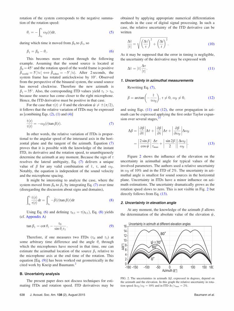
Figure 2 shows the influence of the elevation on the
uncertainty in azimuthal angle for typical values of the
involved parameters. The authors used a relative uncertainty
in xb of 10% and in the ITD of 2%. The uncertainty in azi-
muthal angle is smallest for sound sources in the horizontal
plane. Uncertainty in ITDs have a minor influence on azi-
muth estimations. The uncertainty dramatically grows as the
rotation speed slows to zero. This is not visible in Fig. 2 but
directly follows from Eq. (13).
2. Uncertainty in elevation angle
At any moment, the knowledge of the azimuth b allows
the determination of the absolute value of the elevation w,
FIG. 2. The uncertainties in azimuth Db, expressed in degrees, depend on
the azimuth and the elevation. In this graph the relative uncertainty in rota-
tion speed Dxb=xb ¼ 10% and in ITD Ds=smax ¼ 2%.
638 J. Acoust. Soc. Am. 138 (2), August 2015 Baumann et al.

independently of any motion of the binaural system.
However, the equations cannot discriminate whether the
sound source is located in the upper or lower hemisphere.
Disregarding the missing sign, uncertainty bounds in eleva-
tion can be estimated by combining Eqs. (1) and (2), in order
to form Eq. (14),
w ¼ arccoss
smax cos b
� �: (14)
The uncertainty in elevation is calculable through Eqs.
(13) and (14),
Dw ¼���� @w@s
����Dsþ���� @w@b
����Db
¼���� 1
sin w cos b
���� Dssmax
þ jcotw tan bjDb: (15)
Figure 3 shows the uncertainty in elevation in function
of the azimuth. Errors strongly depend on the elevation, and
rapidly grow, as b approaches 6p=2. Uncertainty in eleva-
tion is smallest for sound sources that are located on the
frontal plane, and greatest for sound sources located near the
horizontal or the median planes.
C. Experimental applications
In order to study the practical value of the described
dynamic localization model, the equations have been imple-
mented into a digital signal processing device with real-time
capacities. The binaural sensor was composed of two omnidir-
ectional Electret condenser microphones fixed on a rod and
two high gain audio amplifiers (cf. Fig. 4). Spacing 2k between
the microphones was 19.5 cm. The binaural sensor was
mounted on a motorized structure, which was horizontally ro-
tatable at variable angular speed between 0 and p rad/s. A ro-
tary encoder measured angular velocity and position for
control purposes at 0.5� resolution.
Experiments were performed in semi-anechoic room
conditions (empty cinema theater with unknown attenuation
coefficient) at different elevation angles. Sound waves were
emitted by a small music playing radio at a distance of 2 m
ð>12kÞ from the microphones. The digital signal acquisition
and processing device consisted of the National Instruments
(Austin, TX) myRIOTM
embedded hardware device, a dual-
core real-time system based on a customizable field pro-
grammable gate array (FPGA).
ITDs were extracted from digitized audio signals by
finding the peak in the running cross-correlation function, as
proposed by Sayers and Cherry.22 In contrast to the method
applied by these authors, a sliding rectangular time-window
of 10 ms was used instead of the original exponential win-
dow. Because timing was critical, especially during fast
rotations of the binaural system, the normalized cross-
correlation function was calculated in the time domain
applying a fast recursive algorithm23 that allowed to produce
ITD at the audio sampling frequency fs¼ 20 kHz. Also, the
resolution in ITD measurement was 1=fs. In order to elimi-
nate bad cues, ITD values were prefiltered with an adaptive
digital filter using the degree of coherence as a weight (cf.
Blauert,16 p. 201). The windowing and prefiltering was about
40 ms. In the case of a rotation speed of 1 rad/s, this signified
an additional uncertainty less than 2.5� in appreciation of the
angle /. Such delay effects in localization have been
observed with human listeners. The existence of binaural
sluggishness suggests that ITD appreciation requires some
processing time in natural hearing as well. Grantham and
Wightman24 evaluate this delay between 44 and 243 ms.
ITDs were differentiated using a first-order polynomial
low-pass filter that was especially designed for the purpose.
Numerical differentiation requires particular precaution, as
the involved operations inevitably introduce truncation and
round off errors that may become excessively high.25
Moreover, because the underlying ITD function sðtÞ is
unmodeled, error-prone and susceptible to noise, simple
methods for computing the numerical derivative were not
helpful. Therefore, a least-square smoothing algorithm26 was
used, in order to guarantee sufficient noise suppression, low
distortion and zero-phase characteristics in the relevant
angular frequency band. This feature was essential, in order
to prevent that the filtering process would generate malign
FIG. 3. This graph evaluates the uncertainty in elevation Dw in function of
the azimuth at different elevation angles. (Identical conditions as explained
in Fig. 2.)
FIG. 4. The picture shows the steerable binaural system made of LEGOTM
parts, microphones, amplifiers and uncased FPGA-based digital signal proc-
essing (DSP) device.
J. Acoust. Soc. Am. 138 (2), August 2015 Baumann et al. 639

phase shifts of the ITD derivative _sðtÞ with respect to sðtÞ,which would cause misinterpretations of sound direction.
Applying Gauss’ method of the least-squares, under the
assumption of constant time steps Dt, a synchronized estima-
tion at current time ti ¼ iDt of the derivative is given by the
following discrete polynomial function p½i� for M consecutive
past values of the difference quotient q½j� ¼ ðs½j� � s½j� 1�Þ=Dt (cf. Appendix E),
p i½ � ¼
XM�1
j¼0
6j� 2 M � 2ð Þ� �
q j½ �
M M þ 1ð Þ : (16)
In order to reduce the number of computations for large
values of M, the filter was modified as follows.
The function, Eq. (16), can be rewritten,
p i½ � ¼ 6Siq i½ � � 2 M � 2ð ÞSq i½ �M M þ 1ð Þ ; (17)
where at any time index i the summations Sq and Siq are
computed upon the latest M values of q,
Sq½i� ¼XM�1
j¼0
q½j� and Siq½i� ¼XM�1
j¼0
jðq½j�Þ: (18)
These sums can be calculated easily and independently
of M (in terms of computing time) with Eq. (19), which at
any time index i, exclusively considers the effects of the de-
parture of the oldest and the arrival of the most recent values
of the difference quotient stored in an M-sized first-in, first-
out (FIFO) data buffer with circular index,
Sq½i� ¼ Sq½ði� 1Þmod M� � qold½i� þ qnew½i�;Siq½i� ¼ Siq½ði� 1Þmod M� � Sq½i� þMðqnew½i�Þ: (19)
(Note that the correctness of this algorithm can be dem-
onstrated without difficulty by induction.)
Figure 5 shows typical filtered measurements of ITD,
ITD derivative, and rotation speed. The measurements were
made at elevation w¼ 0. The robotic system was programmed
to perform a full revolution of the binaural baseline at differ-
ent angular speeds. Figure 6 displays the results of the estima-
tions that have been made by applying the model equations of
this paper. Visibly, the azimuth is well estimated in compari-
son with the measured position [standard deviation in azimuth
is rðb;w¼0Þ ¼ 0:2 rad]. By contrast, although expectedly,
because of the propagation of errors, the elevation of w¼ 0 is
estimated in the three experiments with mean l1 ¼ 0:6 rad
(standard deviation, r1 ¼ 0:3), l2 ¼ 0:4 rad ðr2 ¼ 0:4Þ, and
l3 ¼ 0:3 rad ðr3 ¼ 0:4Þ. A further experiment yielded for
FIG. 5. This graph depicts three exem-
plary experiments. ITDs are expressed
as relative values s=smax, and the
derivatives as _s=smax. Angular speed is
referenced to the binaural coordinate
system. Therefore, the sign is positive,
although the rotation of the binaural
system has been performed clockwise.
FIG. 6. This graph compares the calcu-
lated azimuth values with the reference
values recorded by the rotary encoder.
As expected for sound sources in the
horizontal plane, elevation estimations
present large errors during most of the
time.
640 J. Acoust. Soc. Am. 138 (2), August 2015 Baumann et al.
w ¼ 0:5 rad, rðb;w¼0:5Þ ¼ 0:33 rad, and l ¼ 0:6 rad ðr¼ 0:36Þ in elevation, for instance.
In conclusion, the experiments were necessary to find
out that the critical part of the application of the present
model is related to the synchronicity of the ITD function sðtÞand its derivative _sðtÞ, because common methods of numeri-
cal differentiation of noisy signals introduce an undesired
delay between both functions. The results of the tests con-
firmed that the method yields excellent estimations of the
azimuth in the case of horizontal rotations with growing
errors as the elevation is increased. The method provides
rather bad estimations of the elevation, which improve with
rising elevation at the cost of the azimuthal measurement.
III. MOTION AND BINAURAL DOPPLER EFFECT
In the context of binaural hearing, the appearance of the
Doppler effect in combination with head movements or
motion of the sound source in the horizontal plane has been
studied by Jenison,27 who listed first order formulas showing
that source position, velocity and distance are observable
from combined measurements of interaural time delay,
Doppler effect and sound intensity. M€uller and Schnitzler28
stepped further into the subject by trying to find a relation-
ship between the interaural time delays and the Doppler
effect. The authors studied the Doppler effect on the head
considered as a single spot rather than on the binaural system
with two receivers. Neelon and Jenison29 focused on the
comparison of translatory and rotational source movements.
From observation they concluded that a source that is rotat-
ing around a binaural system does not produce any noticea-
ble Doppler shift. The present paper will prove evidence that
the Doppler shift exists in spite of these results. Only it is
very weak, in the case of slow rotations, as applied by
Neelon and Jenison.29 Iwaya et al.30 developed a rather com-
plex algorithm based on head-related impulse responses
(HRIRs) that adds the Doppler shift to the computations of
time delays. Kumon and Uozumi31 proposed an auditory sys-
tem using an extended Kalman filter (EKF), which fuses the
motion of a mobile robot platform with the sensory informa-
tion of a binaural ITD detector carried by the robot. The
applied model included the Doppler shift in the calculations.
In Sec. III A, three special cases of motion will be stud-
ied: (1) rotations of the binaural system (with a stationary
sound source); (2) rotations of the sound source about the
center (with a stationary binaural system); and (3)
translations of the sound source in parallel to the binaural
baseline (again with the binaural system staying stationary).
Finally, (4) the general case of an arbitrary trajectory of the
sound source will be investigated. The present developments
will prove that the Doppler shift between the binaurally per-
ceived waves and the first derivative of the interaural time
delay are equivalent. It must be recognized that motion is
described in the plane (R, L, S) and that the sound distance is
greater than 12k, so that the true sound direction coincides
with the slope of the asymptote of the related hyperbola of
confusion (/ ’ u) (cf. Fig. 8).
A. Theory
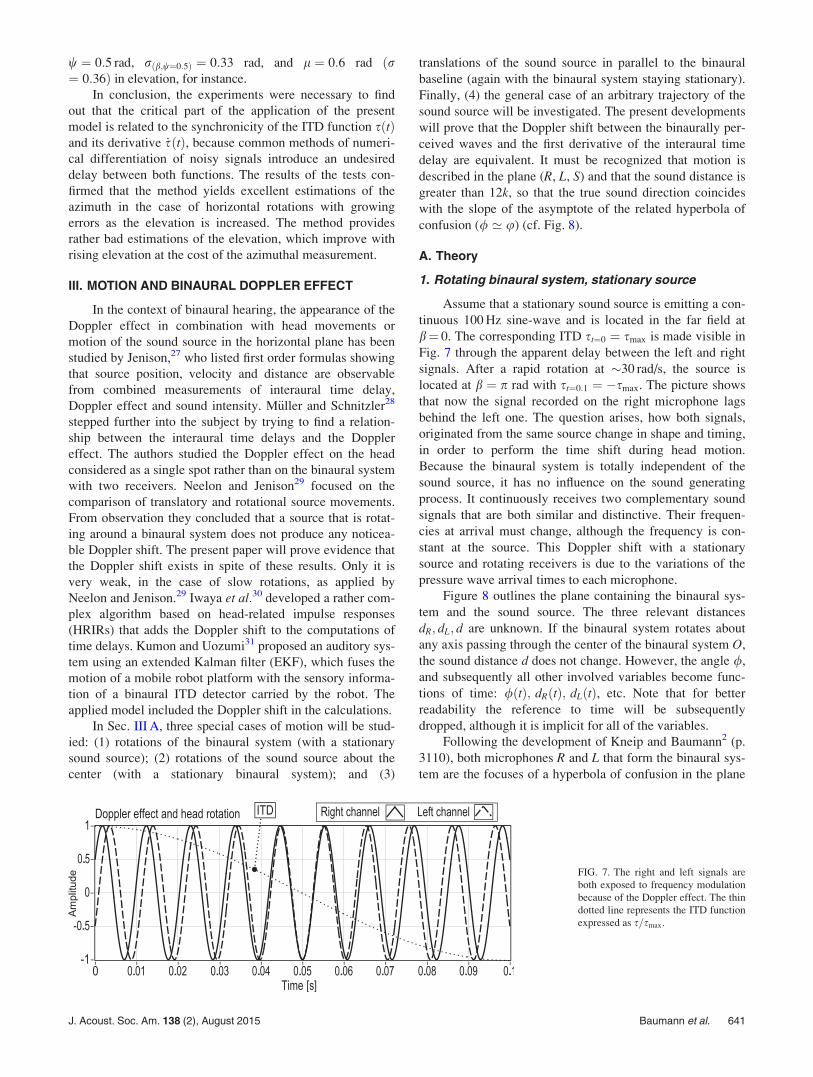
1. Rotating binaural system, stationary source
Assume that a stationary sound source is emitting a con-
tinuous 100 Hz sine-wave and is located in the far field at
b¼ 0. The corresponding ITD st¼0 ¼ smax is made visible in
Fig. 7 through the apparent delay between the left and right
signals. After a rapid rotation at �30 rad/s, the source is
located at b ¼ p rad with st¼0:1 ¼ �smax. The picture shows
that now the signal recorded on the right microphone lags
behind the left one. The question arises, how both signals,
originated from the same source change in shape and timing,
in order to perform the time shift during head motion.
Because the binaural system is totally independent of the
sound source, it has no influence on the sound generating
process. It continuously receives two complementary sound
signals that are both similar and distinctive. Their frequen-
cies at arrival must change, although the frequency is con-
stant at the source. This Doppler shift with a stationary
source and rotating receivers is due to the variations of the
pressure wave arrival times to each microphone.
Figure 8 outlines the plane containing the binaural sys-
tem and the sound source. The three relevant distances
dR; dL; d are unknown. If the binaural system rotates about
any axis passing through the center of the binaural system O,
the sound distance d does not change. However, the angle /,
and subsequently all other involved variables become func-
tions of time: /ðtÞ; dRðtÞ; dLðtÞ, etc. Note that for better
readability the reference to time will be subsequently
dropped, although it is implicit for all of the variables.
Following the development of Kneip and Baumann2 (p.
3110), both microphones R and L that form the binaural sys-
tem are the focuses of a hyperbola of confusion in the plane
FIG. 7. The right and left signals are
both exposed to frequency modulation
because of the Doppler effect. The thin
dotted line represents the ITD function
expressed as s=smax.
J. Acoust. Soc. Am. 138 (2), August 2015 Baumann et al. 641

(R, L, S), and the angle / representing the slope of the char-
acteristic asymptote of that hyperbola is defined by
cos / ¼ dL � dR
2k¼ cs
2k(20)
with
s ¼ dL � dR
c: (21)
The variables may be differentiated with respect to time,
_s ¼ 1
c
d
dtdLð Þ �
d
dtdRð Þ
� �: (22)
If dL or dR are decreased, the respective microphone verges
on the sound source. Therefore, let
vL ¼ �d
dtdLð Þ;
vR ¼ �d
dtdRð Þ: (23)
(It is assumed here that, depending on the direction of
motion on the radial axes, vL ¼ 6k~vLk and vR ¼ 6k~vRk.)Finally, combining these equations results in
_s ¼ vR � vL
c: (24)
Assuming that a pure tone is emitted by the source with
frequency fA, the wavelengths are the same at the source kA
and at the microphones (kR and kL), because the sound
source is stationary in the fluid medium. However, as the
microphones are moving, the speed of sound is virtually
increased (or decreased) by the speeds vR and vL, the fre-
quencies fR and fL must change accordingly,
kR ¼ kA;
cþ vRð ÞfR
¼ c
fA
) fR ¼ 1þ vR
c
� �fA
and similarly fL ¼ 1þ vL
c
� �fA: (25)
Subtracting these equations leads to an expression of the bin-
aural Doppler shift,
fR � fLfA
¼ 1
cvR � vLð Þ ¼ _s: (26)
The role of the unknown source frequency fA in this equation
is to set up the magnitude of the frequency shift.
The law of cosines yields
dR ¼ffiffiffiffiffiffiffiffiffiffiffiffiffiffiffiffiffiffiffiffiffiffiffiA� B cos u
p’
ffiffiffiffiffiffiffiffiffiffiffiffiffiffiffiffiffiffiffiffiffiffiffiA� B cos /
p;
dL ¼ffiffiffiffiffiffiffiffiffiffiffiffiffiffiffiffiffiffiffiffiffiffiffiAþ B cos u
p’
ffiffiffiffiffiffiffiffiffiffiffiffiffiffiffiffiffiffiffiffiffiffiffiAþ B cos /
p;
A ¼ k2 þ d2;
B ¼ 2kd; (27)
d
dtdRð Þ ¼ fR
_/ tð Þsin / tð Þ with
fR ¼kd
d
ffiffiffiffiffiffiffiffiffiffiffiffiffiffiffiffiffiffiffiffiffiffiffiffiffiffiffiffiffiffiffiffiffiffiffiffiffiffiffiffi1þ k2
d2� 2k
dcos / tð Þ
r : (28)
Important note: Eq. (28) is only true, because k and d are
constants,
) limd!1
fR ¼ k: (29)
Therefore, for sufficiently large d compared to k,
vR ¼ �k _/ðtÞ sin /ðtÞ; (30)
and similarly
vL ¼ þk _/ðtÞ sin /ðtÞ; (31)
whence
vL ¼ �vR: (32)
Applying Eq. (25),
fR þ fL ¼ fA 2þ vR þ vL
c
� �¼ 2fA ) fA ¼
fR þ fL2
:
(33)
Finally, by combining Eqs. (26) and (33), the derivative
of the ITD function may be written as the binaural Doppler
equation,
_s ¼ 2fR � fL
fR þ fL: (34)
In conclusion, rotations of the binaural system in any
plane produce relative changes of frequency that are equal in
all frequency band for a source away from the microphones.
2. Rotating sound source, stationary microphones
The development of the binaural Doppler equation from
Sec. III A 1 needs to be reconsidered here, because the
FIG. 8. A rotation of the binaural system in the plane (R, L, S) with the
involved distances and radial speeds. The picture emphasizes the true sound
direction u and the slope of the cone of confusion /, which coincide for
sound sources in the far field.
642 J. Acoust. Soc. Am. 138 (2), August 2015 Baumann et al.
conditions are not the same in the case of a moving sound
source and immobile binaural system (cf. Fig. 9). The wave-
lengths at the source kA and the receivers kR and kL are no
longer identical, because the source is moving in the fluid me-
dium. For instance, if the source is moving away from the
right receiver at speed vSR ¼ �vR, the wavelength of the sig-
nal generated at the source is lengthened by the traveled dis-
tance within the duration of one cycle (note that vSL ¼ �vL):
kR ¼ kA �vR
fA; kL ¼ kA �
vL
fA) fR ¼ fA 1� vR
c
� ��1
;
fL ¼ fA 1� vL
c
� ��1
: (35)
If the involved speeds are much smaller than the speed
of sound, the binomial series approximation can be applied,
1þ qð Þa � 1þ aq; if q� 1
) fR � fL ¼ fA 1þ vR
c� 1þ vL
c
� �� �: (36)
Because the development of Eqs. (27) to (33) can be
applied to a rotating sound source and stationary micro-
phones, the Doppler shift obeys the same equations as dis-
cussed in Sec. III A 1,
fR � fLfA
¼ 1
cvR � vLð Þ ¼ _s; (37)
which leads to
) _s ¼ 2fR � fL
fR þ fL: (38)
In conclusion, both cases of rotation, either with rotating
auditory system, or with rotation of the source, produce the
same Doppler shift.
3. Shifting sound source, stationary microphones
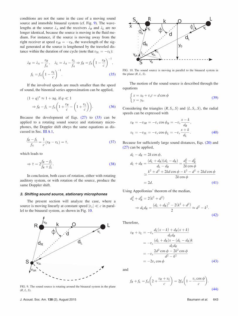
The present section will analyze the case, where a
source is moving linearly at constant speed jvxj � c in paral-
lel to the binaural system, as shown in Fig. 10.
The motion of the sound source is described through the
equations
x ¼ x0 þ vxt ¼ d cos /y ¼ y0:
�(39)
Considering the triangles ðR; Sx; SÞ and ðL; Sx; SÞ, the radial
speeds can be expressed with
vR ¼ �vSR ¼ �vx cos /R ¼ �vxx� k
dR;
vL ¼ �vSL ¼ �vx cos /L ¼ �vxxþ k
dL: (40)
Because for sufficiently large sound distances, Eqs. (20) and
(27) can be applied,
dL � dR ¼ 2k cos /;
dL þ dR ¼dL þ dRð Þ dL � dRð Þ
dL � dR¼ d2
L � d2R
2k cos /
’ k2 þ d2 þ 2kd cos /� k2 � d2 þ 2kd cos /2k cos /
¼ 2d: (41)
Using Appollonius’ theorem of the median,
d2L þ d2
R ¼ 2 k2 þ d2ð Þ
) dLdR ¼dL þ dRð Þ2 � 2 k2 þ d2ð Þ
2� d2 � k2:
(42)
Therefore,
vR þ vL ¼ �vxdL x� kð Þ þ dR xþ kð Þ
dLdR
¼ �vxdL þ dRð Þx� dL � dRð Þk
dLdR
¼ �vx2d2 cos /� 2k2 cos /
d2 � k2
¼ �2vx cos / (43)
and
fR þ fL ¼ fA 2þ vR þ vL
c
� �¼ 2fA 1� vx cos /
c
� �:
(44)FIG. 9. The sound source is rotating around the binaural system in the plane
(R, L, S).
FIG. 10. The sound source is moving in parallel to the binaural system in
the plane (R, L, S).
J. Acoust. Soc. Am. 138 (2), August 2015 Baumann et al. 643

Hence
fA ¼ 1� vx cos /c
� ��1fR þ fL
2: (45)
In this equation, vx is supposed to be small in comparison to
c, so that the first factor can be considered as 1. Because Eq.
(37) is applicable here, the Doppler equation becomes
_s ¼ 2fR � fLfR þ fL
: (46)
In conclusion, slow parallel shifts of the binaural system
obey the same binaural Doppler rule as rotations.
4. Arbitrary trajectory of the sound source, stationarymicrophones
The motion of the sound source on an arbitrary trajec-
tory in the plane (R, L, S) with speed vector~v ¼~vx þ~vy and
k~vk � c can be described with (cf. Fig. 11) the following:
x ¼ d cos /; _x ¼ vx;
y ¼ d sin /; _y ¼ vy; (47)
where, depending on the direction of motion on the x or yaxis,
vx ¼ 6k~vxk and vy ¼ 6k~vyk: (48)
The distance to the sound source is not necessarily constant,
so (cf. Appendix B),
d ¼ffiffiffiffiffiffiffiffiffiffiffiffiffiffiffiffiffiffix2 þ y2ð Þ
p;
_d ¼ vx cos /þ vy sin /;
/ ¼ arctany
x
� �;
_/ ¼ vy cos /� vx sin /d
: (49)
The distances to the microphones are defined by
dR ’ffiffiffiffiffiffiffiffiffiffiffiffiffiffiffiffiffiffiffiffiffiffiffiA� B cos /
p;
dL ’ffiffiffiffiffiffiffiffiffiffiffiffiffiffiffiffiffiffiffiffiffiffiffiAþ B cos /
p(50)
with
A ¼ k2 þ d2;
B ¼ 2kd (51)
and
_A ¼ 2d _d ;
_B ¼ 2k _d : (52)
The radial speed vR may be expressed with (cf. Fig. 11 and
Appendix C)
vR ¼ �vSR ¼ � _dR
¼ � d _d � kvx
dR: (53)
And similarly,
vL ¼ �d _d þ kvx
dL: (54)
Therefore, applying Eq. (41) and Appolonius’ theorem [cf.
Eq. (42) and Appendix D]
vR þ vL ’ �2ðvx cos /þ vy sin /Þ: (55)
Finally, and similarly to Eq. (45),
fA ¼ 1� vx cos /þ vy sin /c
� ��1fR þ fL
2’ fR þ fL
2;
(56)
and from Eq. (37),
_s ¼ 2fR � fL
fR þ fL: (57)
In conclusion, the binaural Doppler equation is applicable
for any kind of motion of the sound source given the
involved speeds are much smaller than the sound velocity.
B. Applications
1. Generating a binaural image
The Doppler equations developed so far describe the
relationship between the binaurally received frequencies and
the ITD derivative. These equations may serve for the simu-
lation of motion in the context of binaural hearing.
Assume that a sound source in the far field is emitting a
pure tone of constant angular frequency xA ¼ 2pfA and zero
phase. The signal amplitude is 1,
sAðtÞ ¼ sin xAt: (58)FIG. 11. The sound source is moving into an arbitrary direction in the plane
(R, L, S).
644 J. Acoust. Soc. Am. 138 (2), August 2015 Baumann et al.

Furthermore suppose that there are no signal losses and that
the binaural system is rotating in the plane (R, L, S) with
angular frequency x/ðtÞ ¼ _/ðtÞ. (Note that the function /ðtÞmay be an arbitrary continuous function of time.)
The generated signals are the results of complementary
frequency modulations of the source signal. Applying Eqs.
(25), (30), and (31), the instantaneous frequencies can be
expressed with
fR tð Þ ¼ 1� k
cx/ tð Þsin / tð Þ
� �fA
¼ 1� smax
2x/ tð Þsin / tð Þ
� �fA ¼ 1þ _s
2
� �fA;
fL tð Þ ¼ 1� _s2
� �fA: (59)
According to the rules of frequency modulation (cf.
Hartmann32), the signal received at the right microphone
changes to
sR tð Þ ¼ sin xA
ðt
0
1þ _s2
dt
!
¼ sin xA tþ s2
� �¼ sin xA tþ smax
2cos / tð Þ
� �:
(60)
Note that the integration constant has been dropped.
Similarly,
sL tð Þ ¼ sin xA t� s2
� �
¼ sin xA t� smax
2cos / tð Þ
� �: (61)
In the case of a constant angular frequency x/, the
sound direction changes according to the equation
/ðtÞ ¼ /0 þ x/t. Figure 12 shows binaural signals that have
been synthesized by applying Eqs. (60) and (61) to each
component of a complex sound signal.
In conclusion, because any desired physical motion of
the sound source can be analytically transformed into varia-
tions of the compound angle /, the developed frequency and
phase equations may be applied for the generation of binau-
ral sound signals. If the constructed sound signals are pre-
sented to a subject via headphones, it is likely that the
impression of source motion will be perceived. However, as
neither back/front nor up/down ambiguity is resolved, only
lateralization will be possible (cf. Plenge33).
2. Constructing a binaural beat
The important relationship described in Eq. (34) may be
illustrated through an experiment known in psychoacoustics
as the binaural beat (cf. Rayleigh,34 Licklider et al.,35 and
Akeroyd36). A typical form of the binaural beat consists in
presenting a 500 Hz sine wave to one ear and a 501 Hz sine
wave to the other (first curve in Fig. 13). Because the fre-
quency difference is very small, humans do not perceive two
separate tones. Instead a single tone is heard, which seems to
move across the head at a rate of 1 Hz from one side to the
other, then flip back, and restart its virtual motion. Because
the appreciation of direction reaches its extrema / ¼ 0; pat smax and �smax, respectively, ITDs have been clipped in
Fig. 13.
This perception of motion directly follows from the bin-
aural Doppler shift equation Eq. (34). In fact, the time lag
between both signals (¼ITD), induced by the slightly shorter
wavelength of one signal, increases at a constant rate, until
both signals are in phase again.
FIG. 12. The right and left signals
have been generated by applying the
equations of Sec. III B 1 to each com-
ponent of a complex signal. Similarly
to Fig. 7, the thin dotted line represents
the ITD function expressed in s=smax.
FIG. 13. Binaural beat experiment.
Two pure tones were generated with
frequencies 500 and 501 Hz (1000 and
1002 Hz). Each signal was recorded at
the opposite input of the binaural sys-
tem. ITDs were calculated through the
running cross-correlation method. The
graph depicts the relative ITD values
s=smax, bounded to the interval
ð�1; 1Þ. In this experiment, the micro-
phone spacing 2 k was 17 cm.
J. Acoust. Soc. Am. 138 (2), August 2015 Baumann et al. 645

Assuming that the microphone spacing 2k ¼ 17 cm,
speed of sound c¼ 343 m/s, fR¼ 501 Hz and fL¼ 500 Hz, the
ITD derivative equals
_ssmax
¼ 2
0:17=c
1
1001� 4 s�1: (62)
Saberi37 mentions that in a complex tone, for a higher
frequency component to maintain the same rate of change in
interaural delay as a lower component, the difference in fre-
quency at the contralateral ear must be proportionately
larger. The factor of proportionality can easily be determined
by rearranging Eq. (34),
fR ¼2þ _s2� _s
fL: (63)
In the example of Eq. (62), the factor of proportionality
in Eq. (63) is 1.002. Therefore, if fL¼ 1000 Hz, the contralat-
eral frequency must be fR¼ 1002 Hz. The second curve in
Fig. 13 shows that, in the case of these frequencies, the rate
of change in ITDs is the same as for 500 and 501 Hz.
However, the appreciation of laterality changes, because at
1 kHz, the signals are out of phase by 180� after 0.25 s. At
500 Hz, this phase shift is reached only after 0.5 s.
In conclusion, the binaural Doppler equation shows that
binaural pitch differences are directly related to dynamic
sound localization.
IV. DISCUSSION
From the epistemological point of view this work
clearly follows a deductive method by attempting to develop
a model for binaural localization of sound that does not pri-
marily rely on empirical data, but on a mathematical con-
struct. The presented model requires a few scaffolding
conditions. The first requirement consists of the (over)sim-
plification of the binaural system to a couple of acoustic
receivers in the free field. Such a system does not exist in na-
ture, nor can it be made artificially. Even with the best
design, real microphones are not reduced to infinitesimal
spots. Acoustic signals are never generated on such a spot ei-
ther. Sound waves represent complex phenomena that are
affected by diffraction in the presence of a head causing im-
portant bias to the fundamental formula relating ITDs to the
slope of the cone of confusion [Eq. (2)]. For that reason
Lambert11 and Duda et al.38 adapted this equation to spheri-
cal or ellipsoidal heads. Regarding such alternative condi-
tions of the initial geometry, further studies could examine
the present model development from the aspect of relevant
variants on Eq. (2).
Another constraint for this model is the far field assump-
tion, which allows a few essential simplifications in the
equation development. This somehow vague condition has
been made precise with two key sound distances 4k and 12kyielding deviations between the slope of the cone of confu-
sion and the true sound direction less than 1� and 0.1�,respectively.2 Further investigation of the near field could
start from the work by Shinn-Cunningham et al.,39 who
suggest considering a torus of confusion for sound sources
within the listeners reach.
An additional implicit assumption in the present paper
is that acoustic signals received by the microphones are iden-
tical in shape and spectrum, except for the modulation
effects due to the Doppler shift and the time delays caused
by path differences of arrival. In all of the practical experi-
ments made during the development of this work, it
appeared that in ordinary room environments this condition
could not be reliably controlled. In fact, disturbances such as
reverberation interference and standing waves do not neces-
sarily display in the same manner in each of the binaurally
received signals, mostly because the microphones occupy
different locations in space, introducing unpredictable errors
in ITD measurements. Hartmann40 reports that the quality of
sound localization in rooms depends on many different pa-
rameters such as direct-signal-to-reverberant-noise ratio,
room geometry, and presence of strong attack transients.
This explains the choices of an empty cinema theater as the
room environment, and a music playing radio as the sound
source used in the experiments of this work. Fortunately, the
application of the normalized cross-correlation function, as
the chosen method for the determination of ITDs, delivers a
measure for the quality of every single ITD estimation. The
maximum of this function defines the degree of coherence
between both audio signals41,42 and may therefore be used as
a weight in an adaptive digital filter, as mentioned in Sec.
II C. Note that the time-domain method deployed in our
experiments did not allow the separation of multiple sound
sources.
In order for Eq. (7) to yield a unique solution for b at
any moment in time, the value of the ITD s may not be zero,
which is equivalent to saying that the sound source may not
be located in the median plane (O, y, z). Also, angular speed
xb must be non-zero as well. However, according to Eqs. (1)
and (2), the trivial case where s¼ 0, yields b ¼ 6p=2.
Moreover, because Eq. (4) always holds, the sign is resolved
in this equation, if the binaural system is moving with a
known direction of rotation.
The analysis of error propagation in Sec. II B unveiled
that in the described model, uncertainty in azimuth dramati-
cally grows as the horizontal rotation speed slows to zero.
This does not necessarily apply to human hearing, where dif-
ferent sources of information, such as ITD, ILD, head-
related transfer function (HRTF), visual and motional cues,
come into play. For instance, Hirahara et al.15 showed that
sound localization accuracy in the horizontal or median
plane was better with the head rotating (even for slow rota-
tions) than when the head was stationary. Further experimen-
tal research could focus on the estimation of the error
bounds that are related to human processing of ITD and its
derivative.
If the state of the binaural system is defined by its orien-
tation in space with respect to the location of the static sound
source, there is confusion about the initial definition of the
binaural coordinate system, because only the x axis is
unequivocal. However, as soon as a system rotation is per-
formed, it stands to reason that the plane of rotation should
be chosen as the “horizontal” plane. In this case, the system
646 J. Acoust. Soc. Am. 138 (2), August 2015 Baumann et al.
is observable for both azimuth and elevation except for the
disambiguation about the upper or lower hemisphere.
System observability is seriously affected in the case of
motion of the sound source, which was explicitly excluded
in Sec. II, and reintroduced in Sec. III of this paper. The bin-
aural system cannot draw inferences about the instantaneous
speed of the sound source, and as a consequence, Eq. (7) is
underdetermined. The reference paper by Kneip and
Baumann2 mentions the possibility of completely solving
the localization problem through combined motion sequen-
ces. In the case of source motion, such a sequence could
override the system underdetermination. In fact, if the binau-
ral system is controlled with the source centering algorithm
displayed in Table I, it will always keep the moving sound
source in the median plane by tracking it. Without any refer-
ence to the “world” coordinate system this means that the
source will appear immobile in the binaural reference frame.
Any additional deliberate rotation of the system with known
angular speed will therefore solve the localization problem
within the limits explained in this paper.
The binaural Doppler equation developed in Sec. III
identifies weak pitch differences between the left and right
signals with the variation of ITDs. In other words, a direct
relationship has been established between spectral displace-
ments in the binaurally captured signals and sound localiza-
tion due to system motion. Yet, it can be concluded from
the definition of _s [Eq. (3)] that, at any moment in time,
there is a unique value of the ITD derivative for a known
angular speed and a specific sound direction in each lateral
hemisphere. Therefore, two or more sound sources that are
located on different cones of confusion will produce differ-
ent patterns of the binaural Doppler shift. We predict that
it might be possible to recognize these patterns in spectral
analyses of the auditory scene, which therefore could con-
tribute to the separation of multiple sound sources. A good
starting point for further research might be the work by
Roman and Wang.43
A final note must be addressed about the binaural
Doppler shift. Despite the promising way of determining
ITD derivatives indirectly via pitch differences, the authors
did not follow this approach in their experimental part,
because they considered the field of pitch detection beyond
the scope of the present work.
V. SUMMARY
In the first part, this paper developed the mathemati-
cal model for dynamic sound localization in space in the
case of rotations of the binaural baseline based on the
knowledge of the rotation speed and the differentiation
of ITDs with respect to time, showing that the sound
direction in the plane of rotation is exactly and instanta-
neously determined, whereas its orthogonal direction is
only yielded in magnitude without the specification of its
sign. The paper also evaluated the error propagation
through the established equations, clarifying that uncer-
tainties in the plane of rotation are bounded and mostly
depend on the sound direction in the orthogonal plane
and the rotation speed. By contrast, uncertainties in the
orthogonal plane were proven to grow excessively for
sound sources located either in that plane or in the plane
of rotation. Finally, the work presented experiments, in
order to examine the practical value of the model for
embedded real-time applications. The experiments did
not include comparative studies with other methods, but
focused on the solution of one major issue related to the
approach, namely, the synchronization of ITD values and
the values of the first ITD derivative. The second part
of the paper developed the binaural Doppler equation
stating that the first ITD derivative is equivalent to the
Doppler effect appearing between the two binaural
receivers. This equation was used to describe the com-
plementary frequency modulation taking place at each re-
ceiver and the binaural beat phenomenon in the case of
small frequency differences.
ACKNOWLEDGMENTS
The authors thank Stephanie Malek and Timothy P.
Martin, Department of Mechanical Engineering, Tufts
University Medford, MA.
NOMENCLATURE
Rðk; 0; 0Þ Position of the right microphone, k> 0
Lð�k; 0; 0Þ Position of the left microphone
2k Spacing between the two microphones
c Sound velocity (�343 m/s in air)
Sðx; y; zÞ Sound-source location
Sxyðx; y; 0Þ Orthogonal projection of S on the hori-
zontal plane
Sxðx; 0; 0Þ Orthogonal projection of S on the x axis
s Interaural time delay (ITD)
smax ¼ 2k=c Maximal detectable ITD
_s Derivative of ITD with respect to time
dR; dL; d Distance to sound source equal to
k~RSk; k~LSk; k ~OSkdL � dR ¼ cs Path difference of arrival (c¼ sound
velocity)
vSR, vSL Speed of the sound source toward the
microphones, equal to the derivatives_dR; _dL
vR, vL Speed of the microphones toward the
sound source, equal to �vSR;�vSL
sA Acoustic signal at the source
sR, sL Acoustic signals at the microphones
fA;xA; kA Frequency, angular frequency and
wavelength of the acoustic signal at
its source
fR; kR; fL; kL Frequencies and wavelengths of the acous-
tic signal as detected on each microphone
u 2 ½0; p� True sound direction in the plane (R, L,
S), referred to the origin O/ 2 ½0; p� Slope of the cone of confusion, / ’ u
for sound sources in the far field
/R;/L Sound directions referred to the micro-
phones R, Lx/ ¼ _/ Variation of sound direction in the plane
(R, L, S)
J. Acoust. Soc. Am. 138 (2), August 2015 Baumann et al. 647
w 2 ½�p=2; p=2� Elevation, vertical angle between the
horizontal plane and the sound-source
vector
b 2 ½�p; p� Horizontal angle (¼azimuth), referenced
to the x axis
xb ¼ _b Variation of azimuth over time, i.e., rota-
tion speed about the z axis
hz Rotation angle about the z axis in
“world” referential frame
APPENDIX A: EQUATIONS (8) AND (9)
ðt1
t0
_s tð Þs tð Þ dt ¼
ðt1
t0
� _b tð Þtan b tð Þdt
() lnjs tð Þj� �t1
t0¼ lnj cos b tð Þj� �t1
t0
() ln
���� s1
s0
���� ¼ ln
���� cos b1
cos b0
����() s1
s0
¼ cos b1
cos b0
ors0
s1
¼ cos b0
cos b1
:
Because b0 ¼ b1 þ hz [cf. Eq. (6)], this changes to (provided
s0 6¼ 0; s1 6¼ 0 and hz 6¼ 0)
s0
s1
¼ cos b1 cos hz � sin b1 sin hz
cos b1
¼ cos hz � tan b1 sin hz
() s0
sin hzs1
¼ cot hz � tan b1
() tan b1 ¼ cot hz �s0
sin hzs1
:
APPENDIX B: EQUATION (49)
_/ ¼ x2
x2 þ y2
x _y � _xy
x2
¼ xvy � yvx
d2
¼ vy cos /� vx sin /d
:
APPENDIX C: EQUATION (53)
vR¼�vSR¼� _dR
¼�_A� _B cos/þB _cos/� �
2dR
¼�2d _d� 2k _d cos/�2kd _/ sin/� �
2dR
¼�d vx cos/þvy sin/� �
�k vx cos2/þvy sin/cos/� �
þ k vy sin/cos/�vx sin2/� �
=dR
¼�d vx cos/þvy sin/� �
�kvx
dR¼�d _d�kvx
dR:
APPENDIX D: EQUATION (55)
vR þ vL ¼ �dL d _d � kvx
� �þ dR d _d þ kvx
� �dLdR
¼ � dL þ dRð Þd _d � dL � dRð Þkvx
d2 � k2
’ �2d2 vx cos /þ vy sin /� �
� 2k2vx cos /
d2 � k2
¼ �2 vx cos /þ d2
d2 � k2vy sin /
� �
¼ �2 vx cos /þ 1
1� k2=d2vy sin /
� �
’ �2 vx cos /þ vy sin /� �
:
APPENDIX E: LEAST-SQUARE LOW-PASS FILTER
Equation (16) in Sec. II C is derived according to
Sch€ußler.26 In contrast to the method used by this author, the
low-pass filter is developed here to the first order only, which
is why ordinary algebraic equations appear more appropriate
than the original vector notation.
Assume that s(t) describes a noisy signal in function of
time. A least-square filter for this function can be designed
as a discrete polynomial approximation p½j� that is evaluated
at M values of the input signal s(t), which have been taken at
equal time steps Dt with respect to the current time
tM�1 ¼ ðM � 1ÞDt. The equation of such a first-order poly-
nomial may be written as
sj ¼ sðtjÞ � p½j� ¼ a0 þ a1tj: (E1)
Ultimately, if Dt! 0, the segment defined by p½j� can
be considered as a superposable model for the signal curve
within the same interval. However, because this model is not
correct for finite values of Dt, the best linear fit can be
obtained by minimizing the sum of the squared residuals Rr,
Rr ¼XM�1
j¼0
½sj � ða0 þ a1tjÞ�2: (E2)
The sum Rr is unknown. However, it can be considered
a function of both values a0 and a1, and its minimum can be
found, if both partial derivatives are zeroed:
@Rr
@a0
¼ �2XM�1
j¼0
sj � a0 þ a1tjð Þ½ � ¼ 0
@Rr
@a1
¼ �2XM�1
j¼0
tj sj � a0 þ a1tjð Þ½ � ¼ 0:
8>>>>>><>>>>>>:
(E3)
Gauss’s method of the least-squares yields a0 and a1 as
the solution of the system of equations that follows from Eq.
(E3),44
648 J. Acoust. Soc. Am. 138 (2), August 2015 Baumann et al.
Ma0 þ ðX
tjÞa1 ¼X
sj Xtj
�a0 þ
Xt2j
�a1 ¼
Xtjsj:
8<: (E4)
Using the summation terms c1 ¼P
tj; c2 ¼P
t2j , and
c3 ¼ Mc2 � c21, the solutions for a0, a1 may be written as
a0 ¼c2
Xsj � c1
Xtjsj
c3
;
a1 ¼MX
tjsj � c1
Xsj
c3
: (E5)
Under the assumption of constant Dt, the terms of Eq. (E5)
may be rewritten,
c1 ¼XM�1
j¼0
tj ¼XM�1
j¼0
jDt ¼ DtXM�1
j¼0
j¼! Dtc01;
c2 ¼XM�1
j¼0
t2j ¼ Dt2
XM�1
j¼0
j2¼! Dt2c02;
c3 ¼ Mc2 � c21 ¼ Dt2ðMc02 � c021 Þ¼
!Dt2c03;X
tjsj ¼ DtX
jsj; (E6)
leading to the equations
a0 ¼c02X
sj � c01X
jsj
c03;
a1 ¼MX
jsj � c01X
sj
Dtc03(E7)
The summations of consecutive integers and their
squares are standard operations of sequences that can be eas-
ily pre-calculated.
c01 ¼XM�1
j¼0
j ¼ MðM � 1Þ=2;
c02 ¼XM�1
j¼0
j2 ¼ MðM � 1Þð2M � 1Þ=6; (E8)
which is why
a0 ¼2 2M � 1ð Þ
Xsj � 6
Xjsj
M M þ 1ð Þ ;
a1 ¼12X
jsj � 6 M � 1ð ÞX
sj
Dt �M M2 � 1ð Þ : (E9)
Because the polynomial p½j� should be evaluated at tM�1, in
order to yield the most actual estimation,
p M� 1½ � ¼ a0 þ a1 M� 1ð ÞDt ¼
XM�1
j¼0
6j� 2 M� 2ð Þ� �
sj
M Mþ 1ð Þ :
(E10)
This low-pass filtering technique can be developed for
higher orders using Faulhaber’s sums of powers formula (cf.
Knuth45).
1K. Nixdorff, Mathematische Methoden der Schallortung in derAtmosph€are (Mathematical Methods of Sound Localization in theAtmosphere) (Vieweg-Verlag, Braunschweig, Germany, 1977), pp. 5–11.
2L. Kneip and C. Baumann, “Binaural model for artificial spatial sound
localization based on interaural time delays and movements of the interau-
ral axis,” J. Acoust. Soc. Am. 124, 3108–3119 (2008).3C. F. Altmann, E. Wilczek, and J. Kaiser, “Processing of auditory location
changes after horizontal head rotation,” J. Neurosci. 29, 13074–13078 (2009).4J. L. van Soest, “Richtungshooren bij sinusvormige geluidstrillingen”
(“Directional hearing of sinusoidal waves”), Physica (The Hague) 9,
271–282 (1929), available at http://opac.nebis.ch.5G. L. Reid and E. Milios, “Active stereo sound localization,” J. Acoust.
Soc. Am. 113, 185–193 (2003).6H. Wallach, “The role of head movements and vestibular and visual cues
in sound localization,” J. Exp. Psychol. 27, 339–368 (1940).7S. Perret and W. Noble, “The effect of head rotations on vertical sound
localization,” J. Acoust. Soc. Am. 102, 2325–2332 (1997).8F. Whightman and D. J. Kistler, “Resolution of front-back ambiguity in
spatial hearing by listener and source movement,” J. Acoust. Soc. Am.
105, 2841–2853 (1999).9W. R. Thurlow, J. W. Mangels, and P. S. Runge, “Head movements during
sound localization,” J. Acoust. Soc. Am. 42, 489–493 (1967).10P. A. Hill, P. A. Nelson, O. Kirkeby, and H. Hamada, “Resolution of
front-back confusion in virtual acoustic imaging systems,” J. Acoust. Soc.
Am. 108, 2901–2910 (2000).11R. M. Lambert, “Dynamic theory of sound-source localization,” J. Acoust.
Soc. Am. 56, 165–171 (1974).12D. Rao and B. Xie, “Head rotation and sound image localization in the me-
dian plane,” Chin. Sci. Bull. 50, 412–416 (2005).13E. A. Macpherson, “Cue weighting and vestibular mediation of temporal
dynamics in sound localization via head rotation,” Proc. Meet. Acoust. 19,
050131 (2013).14D. Morikawa, Y. Toyoda, and T. Hirahara, “Head movement during hori-
zontal and median sound localization experiments in which head-rotation
is allowed,” J. Acoust. Soc. Am. 133, 3510–3510 (2013).15T. Hirahara, D. Yoshisaki, and D. Morikawa, “Impact of dynamic binaural
signal associated with listener’s voluntary movement in auditory spatial
perception,” J. Acoust. Soc. Am. 133, 3459–3459 (2013).16J. Blauert, Spatial Hearing, revised edition (MIT Press, Cambridge, MA,
1983), pp. 178–202.17E. M. von Hornbostel and M. Wertheimer, “€Uber die Wahrnehmung der
Schallrichtung” (“On the perception of the direction of sound”), Sitzungsber.
K. Preuss. Akad. Wiss. 20, 388–396 (1920), available at https://ia802607.us.
archive.org/33/items/sitzungsberichte1920preu/sitzungsberichte1920preu.pdf.18S. B. Andersson, A. A. Handzel, V. Shah, and P. S. Krishnaprasad, “Robot
phonotaxis with dynamic sound-source localization,” in Proceedings ofthe 2004 IEEE International Conference on Robotics and Automation(2004), Vol. 5, pp. 4833–4838.
19P. X. Zhang and W. M. Hartmann, “Lateralization of sine tones-interaural
time vs phase,” J. Acoust. Soc. Am. 120, 3471–3474 (2006).20A. Portello, P. Danes, and S. Argentieri, “Acoustic models and Kalman fil-
tering strategies for active binaural sound localization,” in Proceedings ofthe 2011 IEEE International Conference on Intelligent Robots andSystems (2011), pp. 137–142.
21M. Grabe, Measurement Uncertainties in Science and Technology(Springer, New York, 2005), pp. 70–90.
22B. M. Sayers and E. C. Cherry, “Mechanism of binaural fusion in the hear-
ing of speech,” J. Acoust. Soc. Am. 29, 973–987 (1957).23U. Meyer-Baese, Digital Signal Processing With Field Programmable
Gate Arrays, 3rd ed. (Springer, New York, 2007), 518 pp.24D. W. Grantham and F. L. Wightman, “Detectability of a pulsed tone in
the presence of a masker with time-varying interaural correlation,”
J. Acoust. Soc. Am. 65, 1509–1517 (1979).25D. R. Kincaid and E. W. Cheney, Numerical Analysis, Mathematics of
Scientific Computing, 3rd ed. (American Mathematical Society,
Providence, RI, 2002), pp. 28–41.26H. W. Sch€ußler, Digitale Signalverarbeitung 2 (Digital Signal Processing
2) (Springer, Heidelberg, Germany, 2010), pp. 376–381.
J. Acoust. Soc. Am. 138 (2), August 2015 Baumann et al. 649

27R. L. Jenison, “On acoustic information for motion,” Ecol. Psychol. 9,
131–151 (1997).28R. M€uller and H.-U. Schnitzler, “Acoustic flow perception in cf-
bats: Properties of the available cues,” J. Acoust. Soc. Am. 105, 2958–2966
(1999).29M. F. Neelon and R. L. Jenison, “The effect of trajectory on the auditory
motion aftereffect,” Hearing Res. 180, 57–66 (2003).30Y. Iwaya, M. Toyoda, and Y. Suzuki, “A new rendering method of
moving sound with the Doppler effect,” in 11th InternationalConference on Auditory Display, Limerick, Ireland (2005) pp.
253–255.31M. Kumon and S. Uozumi, “Binaural localization for a mobile sound
source,” J. Biomech. Sci. Eng. 6, 26–30 (2011).32W. M. Hartmann, Signals, Sound and Sensation (Springer, New York,
1998), 430 pp.33G. Plenge, “On the differences between localization and lateralization,”
J. Acoust. Soc. Am. 56, 944–951 (1974).34Lord Rayleigh, “On our perception of sound direction,” Philos. Mag. 13,
214–232 (1907).35J. C. R. Licklider, J. C. Webster, and J. M. Hedlun, “On the frequency lim-
its of binaural beats,” J. Acoust. Soc. Am. 22, 468–473 (1950).36M. A. Akeroyd, “A binaural beat constructed from a noise,” J. Acoust.
Soc. Am. 128, 3301–3304 (2010).
37K. Saberi, “Fast Fourier-based dsp algorithm for auditory motion
experiment,” Behav. Res. Methods Instrum. Comput. 36, 585–589 (2004).38R. O. Duda, C. Avendano, and V. R. Algazi, “An adaptable ellipsoidal
head model for the interaural time difference,” in Proceedings of the IEEEInternational Conference of the Acoustics, Speech, and Signal Processing(1999), pp. 965–968.
39B. G. Shinn-Cunningham, S. Santarelli, and N. Kopco, “Tori of confusion:
Binaural localization cues for sources within reach of a listener,”
J. Acoust. Soc. Am. 107, 1627–1636 (2000).40W. M. Hartmann, “Localization of sound in rooms,” J. Acoust. Soc. Am.
74, 1380–1391 (1983).41B. Rakerd and W. M. Hartmann, “Localization of sound in rooms. V. bin-
aural coherence and human sensitivity to interaural time differences in
noise,” J. Acoust. Soc. Am. 128, 3052–3063 (2010).42C. Faller and J. Merimaa, “Source localization in complex listening situa-
tions: Selection of binaural cues based on interaural coherence,” J. Acoust.
Soc. Am. 116, 3075–3089 (2004).43N. Roman and D. Wang, “Binaural tracking of multiple moving sources,”
Trans. Audio Speech Lang. Proc. 16, 728–739 (2008).44J. O. Rawling, S. G. Pantula, and D. A. Dickey, Applied Regression
Analysis: A Research Tool, 2nd ed. (Springer, New York, 1998), pp. 3–7.45D. E. Knuth, “Johann Faulhaber and sums of powers,” Math. Comp. 61,
277–294 (1993).
650 J. Acoust. Soc. Am. 138 (2), August 2015 Baumann et al.
Related Documents