Dynamic Asset Allocation Using Systematic Sector Rotation

IT IS

ILLEGAL T

O REPRODUCE T

HIS A

RTICLE IN

ANY F

ORMAT

SPRING 2006 THE JOURNAL OF HEALTH MANAGEMENT 1

The financial markets downturn of2000-2002 has tested a number ofinvestment strategies and raised(again) the question of whether one

can devise a rule to achieve returns abovemarket indices while protecting the capitalinvested. The results obtained by investmentfunds during 2000-2002 suggest that passiveand semipassive investment strategies cannotprotect investors against the negative effect ofa prolonged period of poor economic condi-tions. At the same time, the alternative offeredby active investment strategies, based on theidea of selecting specific stocks or asset classes,has obtained mixed results. Although real estateinvestment trusts (REITs) and funds special-izing in precious metals have been able tomaintain their value at times of falling marketindices, they did not keep pace with the riseof technology stocks in early 2003. Areinvestors really stuck with choosing betweena passive investment strategy and active diver-sification through asset classes within or acrosscountries? We do not think so, and in thisarticle we present the results of a series of sim-ulations that use systematic rotation amongequity sectors as a tool for dynamic asset allo-cation. We test our strategy on U.S. data forthe period 1998-2003. Our aim is not to searchfor a system to “beat the market” but toencourage investors, academics, and fund man-agers to question some of the assumptionscommonly used in investment managementand to investigate with more rigor some of theheuristic methods used by practitioners.

The article is organized as follows. Webegin by reviewing the reference literaturebefore introducing the concept and practiceof dynamic sector rotation. We then presentour experiment: to apply a number of heuristictechniques of sector momentum to a fullyinvested portfolio of sector-specific investments(41 funds of the Fidelity Select Sector family,for which we have data). We first present theempirical results obtained using alternativemeasures of relative strength (rate of change,alpha, and MACD [moving average conver-gence divergence)] indicators) and subse-quently expand our investment strategy to aportfolio composed of shares and cash. Ourresults do not take into account the capitalgains tax regime of the country of the investor.Hence, they do not illustrate the tax efficiencyof strategies of systematic sector rotation, whichmay require the realization of significant short-term net capital gains.

LITERATURE

Although the links among business cycle,sectoral performance, and investment strategyare an obvious area of confluence for financialand economic sciences and investment prac-tice, there is a lack of interaction between thesedisciplines, which results in a significant butseemingly untouched middle ground. Thisstatus quo may be the consequence of the dif-ferent objectives. At the one extreme, the aca-demic and practicing worlds of finance haveexpended much effort in predicting and

Dynamic Asset Allocation UsingSystematic Sector RotationPAOLO SASSETTI AND MASSIMILIANO TANI

MASSIMILIANO TANI

is at the School ofBusiness, University ofNew South Wales at theAustralian Defence ForceAcademy, CampbellACT, [email protected]

PAOLO SASSETTI

is a member of thescientific committee ofRivista Aiaf (Review of theItalian Financial Analysts),Milan, [email protected]

JWM_SP06_Sassetti.qxp 12/28/05 10:02 PM Page 1

IT IS

ILLEGAL T

O REPRODUCE T

HIS A

RTICLE IN

ANY F

ORMAT

accounting for asset price movements. For instance, thefoundation papers of Fama and Schwert [1977], Campbell[1991], Harvey [1991], and Campbell and Ammer [1993]use dividend yields and interest rates to predict excess stockreturns, and the studies of Shiller et al. [1983] and Famaand Bliss [1987] draw parallels between bond returns andterm structures, but they do not explore in any detail themany common threads between financial performance andthe economic cycle. At the other extreme, the economicliterature focuses on much broader and abstract issues aboutthe functioning and efficiency of capital markets.

The status quo notwithstanding, existing work hasgenerally recognized the significant explanatory power ofmacroeconomic variables in determining asset prices. Sincethe early 1970s (e.g., Officer [1973]; Schwert [1989]), aportion of the literature has explored the relationshipbetween investment performance and macroeconomic indi-cators with the explicit intent of improving the predictiveability of underlying forecast models. The typical approachfollowed in these studies, which absorbs the insights of thearbitrage pricing theory, is to treat the aggregate economicvariable as an exogenous black box and include it directlyinto a forecast model. For example, Flavin and Wickens[1998, 2003] include movements in the UK Retail PriceIndex (RPI) to update a portfolio of three UK assets (equity,short-term, and long-term bonds) and find that this invest-ment strategy consistently reduces risk (by more than 20%)for only a marginal reduction in the average return. Bordoand Jeanne [2002] find that monetary policy tools have asignificant impact on asset price movements, suggestingthat a proactive use of monetary policy indicators canenhance returns over the business cycle. In some cases,stock market behavior is also used as a predictor of the eco-nomic cycle (e.g., Moore [1983]).

A variation on this theme is the inclusion of severalmacroeconomic influences (rather than an individual influ-ence) as explanatory variables of stock market movementsin an attempt to fill the “embarrassing gap [that] existsbetween the theoretically exclusive importance of system-atic ‘state variables’ and our complete ignorance of theiridentity” (Chen et al. [1986], p. 384). For instance, Chenet al. [1986] find that industrial production and unantici-pated levels of inflation are significant determinants of pricemovements, unlike consumption and oil prices. Kearneyand Daly [1998], building on Schwert [1990], study marketvolatility using monthly data for movements in industrialproduction, money supply, inflation, the current account,exchange rates, and interest rates and find a significant sta-tistical relationship between all these variables bar exchange

rates1 and movements in stock prices. Still within thisapproach is the study of the functional forms that mayunderpin the relationship between fluctuations in the busi-ness cycle and movements in indices of either aggregatefinancial market activity or individual sectors. Chen [1996],building on the economic chaos literature of Brock andSayers [1998], Ramsey et al. [1990], and DeCoster andMitchell [1991], suggests that the variance of aggregatestock prices is not a pure random walk, as suggested by theefficient market hypothesis, but can largely be explainedby a chaos model of the business cycle. Empirical evidencethat indices do not follow a random walk is provided byEdwards et al. [2003] in a study of price movements insome emerging markets of Latin America and SoutheastAsia since liberalization in the late 1980s and early 1990s.

A major criticism of this approach is its emphasison the response of aggregate indices of financial perfor-mance, which are typically based on asset classes (e.g.,stocks, bonds, and the money market), rather thanexploring the heterogeneous behavior of the sectors thatcompose the economy. Upward and downward swingsof the business cycle and their interactions with the finan-cial markets are studied across asset types and markets (per-haps reflecting an accounting approach to data collection)with minimal reference to the fact that at different stagesalong the cycle different industries will perform betterthan others. Even when the analysis focuses on the rela-tionship between the economy and a particular industry,emphasis seems to be placed on describing the pro- orcounter-cyclical nature of a sector rather than exploitingsuch information with the aim of developing a dynamiccross-sectoral investment strategy. For example, Ross andZisler [1991] and Zisler [1990] discuss the hedging qual-ities achievable with real estate, where returns depresswith high levels of industrial production and surge withhigh consumption. More recently, Sadorsky [2003] foundthat the price volatility of U.S. technology stocks over theperiod 1986–2000 is better explained by own lagged vari-ables and macroeconomic influences are successful pre-dictors of stock market prices at the aggregate level,implying that technology moves in a cyclical fashion, butnot at the same pace as the market as a whole.

Exclusive focus on asset classes rather than a sec-torally based portfolio is also a major limitation of the lit-erature on investment management. Yet, it is due to thisliterature that we know the success of dynamic asset allo-cation strategies in consistently reducing portfolio riskand increasing investment returns. For instance, Brinsonet al. [1986, 1991] show that 90% of the variability of

2 DYNAMIC ASSET ALLOCATION USING SYSTEMATIC SECTOR ROTATION SPRING 2006


IT IS

ILLEGAL T

O REPRODUCE T

HIS A

RTICLE IN

ANY F

ORMAT

portfolio performance and 91.5% of the differential returnsacross pension funds is due to the use of active asset allo-cation strategies. Brennan et al. [1997], Brocato and Steed[1998], and Harloff [1998], among others, report thatstrategic asset allocation produces better risk-adjustedreturns than a passive (buy-and-hold) investment strategy.Among asset allocation techniques, Grauer et al. [1990,1995] compare the success of three classes of investmentestimators (the simple historic or sample estimator, twoshrinkage estimators, and a Capital Asset Pricing Model(CAPM)-based estimator) and find that neither of thetwo shrinkage estimators nor the CAPM based estimatorwas able to outperform the sample estimator.

We believe that the insights of these studies shouldbe explored together as a single research area.

SYSTEMATIC SECTOR ROTATION

Systematic (or dynamic) sector rotation is based onthe idea that the sectors making up the economy do notfollow the same patterns over time but move differentlyfrom one another (e.g., Stovall [1996]). Two main reasonsseem to underpin this behavior. The first is the presenceof fundamentals. Some sectors benefit relative to othersduring the growth phases of the economy (e.g., hotels andleisure), whereas other sectors are relatively better off whenthe economy is in decline (e.g., tobacco). The second reasonis psychological, and it reflects investors’ beliefs about asector’s future performance relative to another or a momen-tarily fashion. Hence, at each point of the economic cycle,there are sectors that have more chances to generate anextra return (or hold value) relative to other sectors or thatare reputed to achieve this result. Systematic sector rotationaims at switching the portfolio regularly so as to capture atleast part of the extra returns that different sectors experi-ence relative to the rest of the market. The ability to iden-tify current and next “hot themes” would give investors thepossibility of outperforming the market.

As suggested by Fowler [1997], the critical issue indynamic asset allocation is to define the guiding rule toidentify ex ante the rotation criteria to follow in switchingamong sectors. Since this guiding rule in discretionaryportfolio management is typically subjective, it is open toquestion. Hence, institutional investors tend to avoid usingdynamic investment strategies, preferring to invest in apredefined mix of asset classes managed by specialists whoseperformances are measured against specific benchmarks.2

Market-timing techniques are a simplified form ofdynamic asset allocation that is popular among individual

investors. They include only two asset classes: shares andcash. Given their simplified nature, they should be lessopen to interpretation. One would therefore expect to seethem commonly used by professional fund managers,though this does not seem to be the case. The reasons forthe modest popularity of these techniques in professionalportfolio management can be summarized as follows:

1. Market-timing techniques are heuristic, with noneof the formal rigor of optimization models. Hence,they have never enjoyed the favor of academics, whotraditionally have preferred using optimization tech-niques despite their most notable limitations, suchas the reliance on static models of the past ratherthan dynamic representations of the present.

2. Given their heuristic rather than scientific nature,these models are tied to the ability, creativity, andintuition of their individual developers. Therefore,their adoption is at odds with the rigid organiza-tional structures and management styles typical oflarge investment firms.

3. Market-timing techniques have typically only twodimensions to the investment: price and time. How-ever, they leave aside the selection of the asset class,which is normally predetermined. The applicationof market-timing uses computerized trading systems,which normally define when and by how much afund manager can be positioned on a specific market,though they do not specify which market or assetclass to choose. This limitation compromises theoptimal criterion that institutional investors set fortheir fund managers (“Who says that these marketsare the most promising/trending at any given time?”).

4. Last but not least, when markets have risen consis-tently with few limited and sudden falls, as from theearly 1980s to 2000, market-timingtechniques haveperformed worse than buy-and-hold strategies. Insti-tutional investors rarely use market-timing tech-niques, and when they do use them have done sofor the purpose of insuring the investment againstthe possibility of disastrous losses rather than in thebelief that they may outperform the market underany conditions.

Despite these limitations, the dynamic nature of thecapital markets and the possibility of new prolonged fallsin the stock market indices suggest that institutionalinvestors might consider introducing more flexibility,adaptability, and readiness to change into their currentpractices.



IT IS

ILLEGAL T

O REPRODUCE T

HIS A

RTICLE IN

ANY F

ORMAT

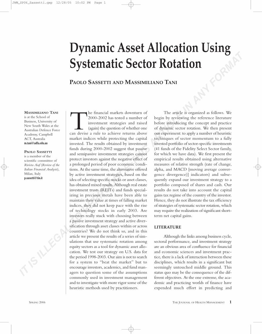
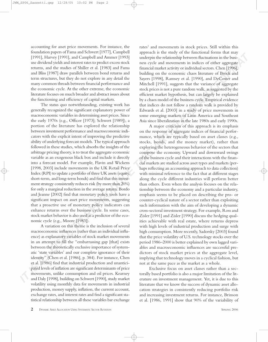
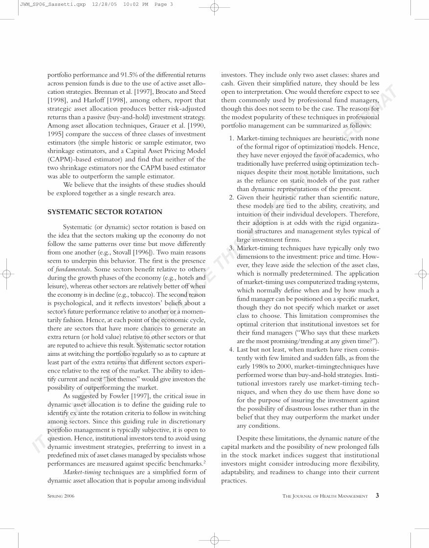
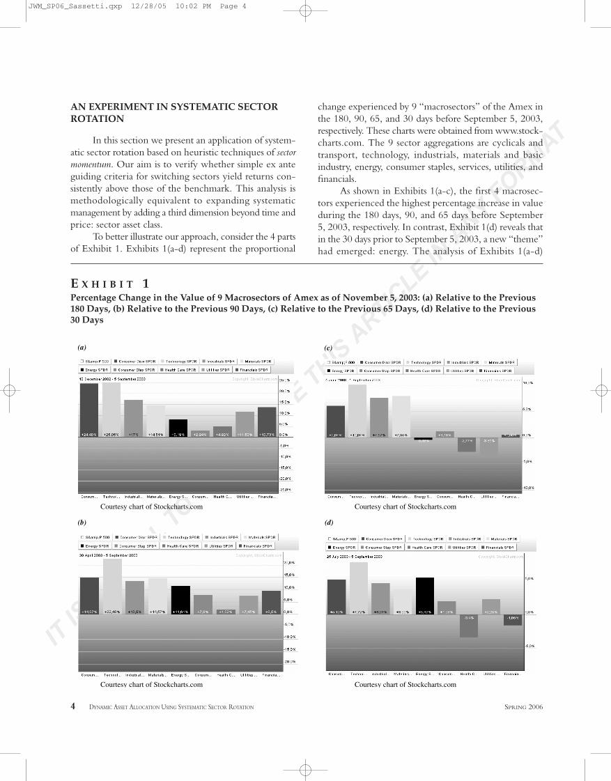
AN EXPERIMENT IN SYSTEMATIC SECTORROTATION

In this section we present an application of system-atic sector rotation based on heuristic techniques of sectormomentum. Our aim is to verify whether simple ex anteguiding criteria for switching sectors yield returns con-sistently above those of the benchmark. This analysis ismethodologically equivalent to expanding systematicmanagement by adding a third dimension beyond time andprice: sector asset class.

To better illustrate our approach, consider the 4 partsof Exhibit 1. Exhibits 1(a-d) represent the proportional

change experienced by 9 “macrosectors” of the Amex inthe 180, 90, 65, and 30 days before September 5, 2003,respectively. These charts were obtained from www.stock-charts.com. The 9 sector aggregations are cyclicals andtransport, technology, industrials, materials and basicindustry, energy, consumer staples, services, utilities, andfinancials.

As shown in Exhibits 1(a-c), the first 4 macrosec-tors experienced the highest percentage increase in valueduring the 180 days, 90, and 65 days before September5, 2003, respectively. In contrast, Exhibit 1(d) reveals thatin the 30 days prior to September 5, 2003, a new “theme”had emerged: energy. The analysis of Exhibits 1(a-d)


(a)

Courtesy chart of Stockcharts.com

(b)


(c)


(d)


E X H I B I T 1Percentage Change in the Value of 9 Macrosectors of Amex as of November 5, 2003: (a) Relative to the Previous180 Days, (b) Relative to the Previous 90 Days, (c) Relative to the Previous 65 Days, (d) Relative to the Previous30 Days


IT IS

ILLEGAL T

O REPRODUCE T

HIS A

RTICLE IN

ANY F

ORMAT

suggests the existence of path dependence (a sort of sectormemory) in the returns of the macrosectors. Such pathdependence drives, at least for a little while, the subsequentoverperformance of these sectors relative to the othermacrosectors. This example is indicative of the fact thatprice movements across sectors do not seem to follow achaotic path. In contrast, they seem to evolve over fairlydefined trends.

Next, we wanted to verify empirically whetherthis phenomenon could be exploited in practice (andnot only recognized ex post) to obtain a total returnabove that of the S&P 500, which we used as a bench-mark. Again, this idea is not new. In the early 1980s,Gil Blake, a trader who became famous for developingtrading systems on mutual funds, noticed that althoughindividual stocks and funds followed a random behavioron a day-by-day basis, some sector funds had a higherlikelihood (approximately 70-80%) of performing in thesame direction for some days after a particularly anom-alous daily change. As he said, “assume you have 99chemical stocks which on average are up 1 or 2 percenttoday, while the broad market is flat. In the very shortrun, this homogenous group of stocks tends to behavelike a school of fish. While the odds of a single chem-ical stock being up tomorrow may be 55%, the odds forthe entire chemical group are much closer to 75%”(Schwager [1992]).

Later, Harloff [1998] showed that a strategy ofdynamic switching among uncorrelated asset classes (e.g.,precious metals, long- and short-term bonds, sector funds,growth funds, international funds) based on relativestrength momentum was very successful in terms of highercompound return and Sharpe ratio relative to a bench-mark composed of aggressive growth funds.

More recently, King et al. [2002] have suggestedthat the long-term persistence in asset class index returnsmay be captured in order to enhance portfolio riskand return vis-à-vis buy-and-hold and constant mix strate-gies.

Consistent with Blake’s original insight, we simu-lated investing in the U.S. market using sector rotation asa dynamic investment device, and we did so for a longerperiod of time. The simulations were run on U.S. marketdata covering the period from January 1, 1998, to Sep-tember 18, 2003. This period includes a market charac-terized by a “bull,” a “distribution,” a “bear,” and a second“bull” trend, therefore covering a complete market cycle.We simulated our strategy using 41 sector funds from theFidelity Select Sector family.3

EMPIRICAL RESULTS

The first set of empirical results was obtained byfully investing in the Fidelity funds. In particular, we sim-ulated investing in the first 1, 2, 3, . . ., 10 and all the 41funds of the series Fidelity Select Sector, picking as aselection criterion the funds with the highest relative strengthin the previous 30, 60, and 90 days. The relative strengthwas calculated using three different indicators:

1. the rate of change, calculated for each fund in theprevious 30, 60, and 90 days, which is a simple mea-sure of price “speed” in the chosen time frame

2. the alpha of the Capital Asset Pricing Model,calculated for each fund using the same time frame,which represents the risk-adjusted return of a fundrelative to the market index

3. the relative strength of each fund with respect to theS&P 500. Specifically, the relative strength of eachfund over the S&P 500 was computed using itsmoving average calculated over a period of 180 daysand then over 3 shorter periods (30, 60, and 90 days).The difference between each of the three shortermoving averages and the one calculated on 180 dayswas interpreted as the relative strength of the fund

The time frames of 30, 60, and 90 days were chosenpurely on the basis of heuristic criteria, with no opti-mization algorithm. We simply assumed that our invest-ments in each fund were held for at least 30 days in ordernot to incur the switch commissions applied by Fidelityfor shorter holding periods (recently Fidelity hasannounced the removal of the front-end load for the SelectSector fund family we used in our simulations). Obvi-ously, the minimum holding period of 30 days is not anoptimal condition. Nor did we apply the stop loss andtrailing stop features, to avoid adding more structure andinterferences with the “natural” dynamics of sector rota-tion to the preliminary simulations we wanted to per-form. This simplified approach was chosen to avoid therisk of overfitting the sector rotation criteria we followedand to provide an unrefined and raw computational outputwith which future work, based on more sophisticatedalgorithms, could be compared.

Our first result indicated that if we had invested anequal amount in each of the 41 funds of the Fidelity SelectSector family at the beginning of January 1998, the resultingportfolio performance at the end of the period would havebeen 37%. The corresponding performance of the S&P500 was 7%. Hence, between 1998 and 2003, the Fidelity



IT IS

ILLEGAL T

O REPRODUCE T

HIS A

RTICLE IN

ANY F

ORMAT

(on average) of the family of funds we used in our tests. Thefollowing sections describe the results of the simulationsobtained following each of the criteria described here.

Using the Rate of Change

The selection of funds based on the rate of changein the previous 30, 60, and 90 days yielded the followingperformance.

Exhibit 2 indicates that choosing a reduced numberof sector funds to invest in at the same time (1-2) does notappear to yield the best returns, possibly because of thenoise signals that characterize the funds with high volatility.The noise leads to exiting from such funds prematurelyafter a sudden fall in prices. The highest return is high-lighted in bold in the exhibit and was obtained followingthe rate of change calculated on the previous 60 days,keeping positions simultaneously in 3 sector funds, and car-rying out on average 26 trades each year, of which 62%yielded a profit. The relatively high proportion of tradesincurring a loss (38%) is neither surprising nor particularlysignificant as the model cannot short trade, and it was alwaysfully invested throughout the period.

Using the Alpha Indicator

The results following a sector rotation based on thealpha indicator using the same time frames (30, 60, and90 days) are reported in Exhibit 3. They appear moreregular and stable than those obtained using the rate of


Number 30 days 60 days 90 days

of funds R.o.C. R.o.C. R.o.C.

1 156% 10% 5%

2 86% 95% 78%

3 37% 215% 84%

4 64% 148% 101%

5 66% 148% 132%

6 69% 144% 121%

7 80% 120% 89%

8 49% 96% 88%

9 72% 110% 99%

10 52% 110% 99%

41 37% 37% 37%

E X H I B I T 2Total Return of a Sector Rotation Strategy Basedon the Rate of Change Indicator


of funds Alpha Alpha Alpha

1 43% 48% 56%

2 81% 44% 67%

3 40% 164% 57%

4 72% 179% 106%

5 92% 186% 149%

6 125% 138% 138%

7 115% 151% 162%

8 110% 116% 141%

9 79% 88% 135%

10 94% 60% 110%

41 37% 37% 37%

E X H I B I T 3Total Return of a Sector Rotation Strategy Basedon the Alpha Indicator

12

34

56

78

910

30 days60 days

90 days

0

50

100

150

200

To

tal R

etu

rn

Number of Funds

Period

E X H I B I T 4Distribution of Total Returns of the Sector RotationModel Based on the Alpha Indicator

Select Sector family of funds experienced an additional30% returns above the S&P 500. It is difficult to believe thatall of the extra performance achieved using sector rotationcan be attributed to this strategy. Part of the strategy’s over-performance may be attributed to the high relative strength


IT IS

ILLEGAL T

O REPRODUCE T

HIS A

RTICLE IN

ANY F

ORMAT

change. The best total return, highlighted in bold, wasobtained using the alpha indicator calculated on the pre-vious 60 days, with 5 funds and 42 trades per annum, ofwhich 56% yielded a profit.

One interesting feature is that with both the alphaindicator and the rate of change, the overperformancerelative to the benchmark rises with the number of fundsinvested, peaks when the number of funds is between 3

and 7, and declines thereafter (see Exhibit 4). At the sametime, the strength line of the equity curve relative to thebenchmark (see later) becomes smoother as the numberof funds invested peaks at the optimal number. Hence,the extra performance of the rotational strategies seemsto become more stable and regular over time. This pat-tern suggests that sector rotation outperforms the bench-mark during speculative phases and “administers” suchgains in subsequent periods, accepting some periods oflimited underperformance.

Using the MACD

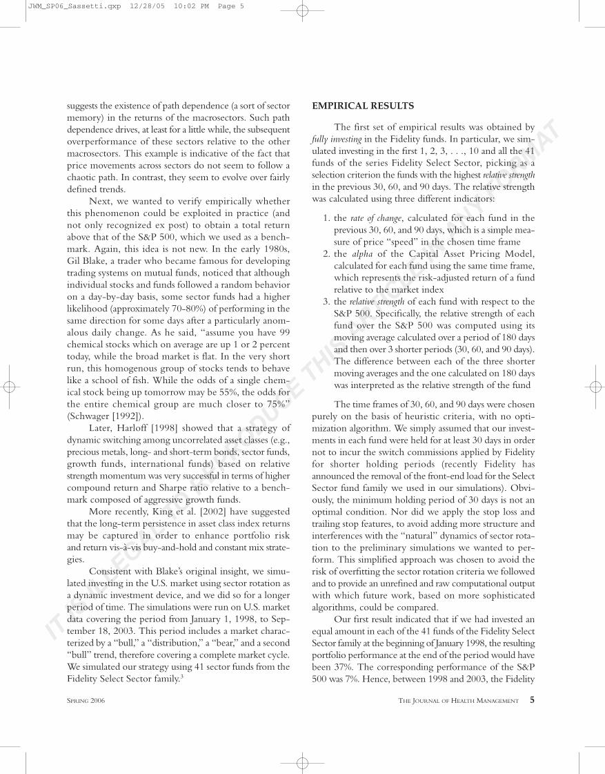
Exhibit 5 shows the results obtained when sectorrotation follows the MACD indicator, calculated over theprevious 30, 60, and 90 days relative to the S&P 500.

This simulation has yielded the most reliable returnsamong those examined so far, in the sense that their dis-tribution “almost” follows the shape of a normal distri-bution, which we take as indicating the absence ofextremely high spikes in the distribution of total returns.This result may be due to the fact that the MACD indexcaptures the strongest and most lasting intermediate sectortrends.4 The best performance test was obtained on therelative strength indicator calculated over the previous 90days, using 5 funds and generating on average 15 tradeseach year, which yielded a profit 52% of the time.

This model withstood the bear market up to mid-2002. Then it lost ground relative to the benchmark. Itsubsequently bounced back in 2003 and gained more than

proportionally relative to the S&P 500 fol-lowing the recovery of the technology sec-tors that took place in early 2003. In fact,at the end of the test (September 18) thismodel held positions in five technologyfunds (Developing Communications�19%, Technology �10%, Networking�13%, Computers �11%, Wireless �1%).

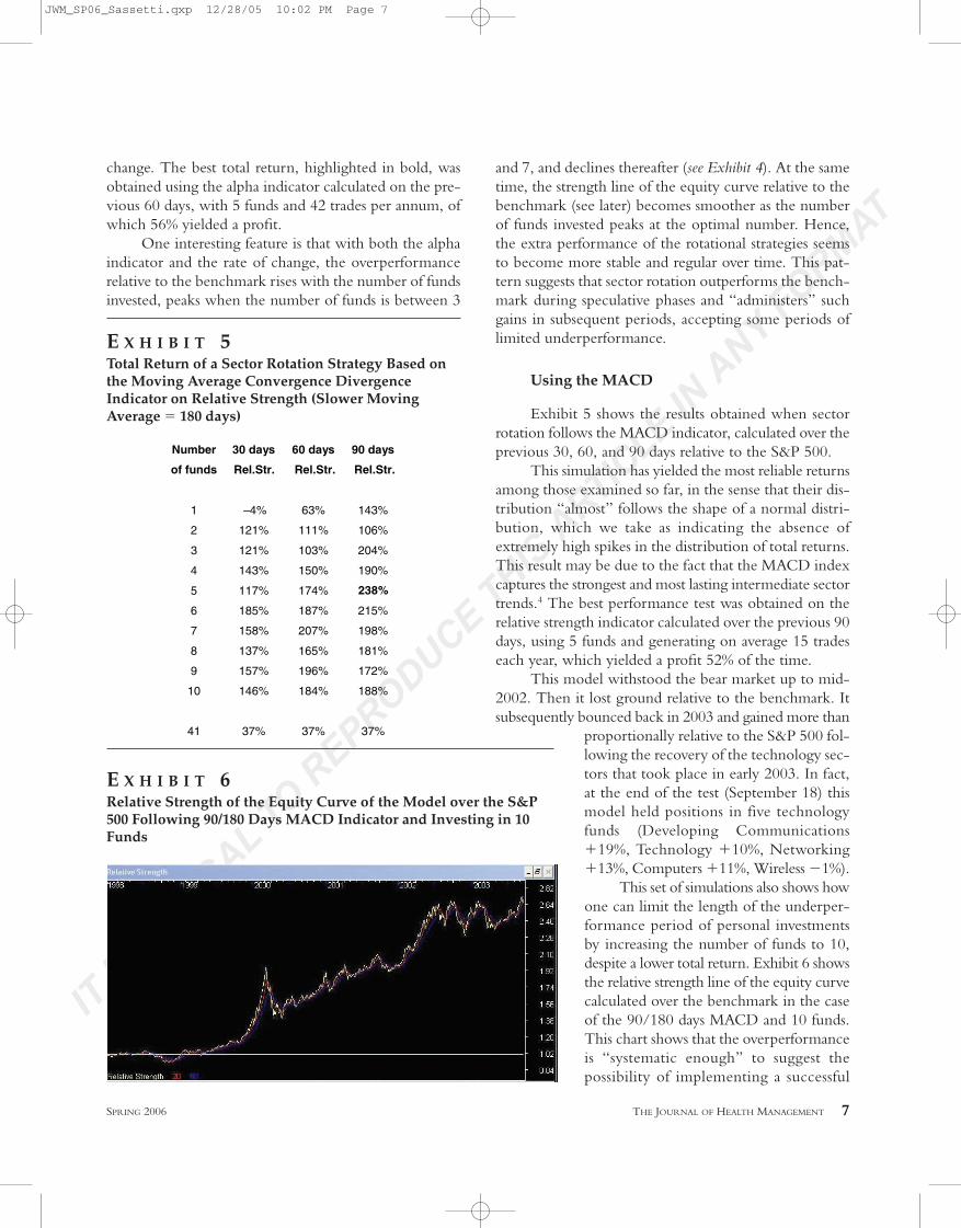
This set of simulations also shows howone can limit the length of the underper-formance period of personal investmentsby increasing the number of funds to 10,despite a lower total return. Exhibit 6 showsthe relative strength line of the equity curvecalculated over the benchmark in the caseof the 90/180 days MACD and 10 funds.This chart shows that the overperformanceis “systematic enough” to suggest thepossibility of implementing a successful



of funds Rel.Str. Rel.Str. Rel.Str.

1 –4% 63% 143%

2 121% 111% 106%

3 121% 103% 204%

4 143% 150% 190%

5 117% 174% 238%

6 185% 187% 215%

7 158% 207% 198%

8 137% 165% 181%

9 157% 196% 172%

10 146% 184% 188%

41 37% 37% 37%

E X H I B I T 5Total Return of a Sector Rotation Strategy Based onthe Moving Average Convergence DivergenceIndicator on Relative Strength (Slower MovingAverage � 180 days)

E X H I B I T 6Relative Strength of the Equity Curve of the Model over the S&P500 Following 90/180 Days MACD Indicator and Investing in 10Funds


IT IS

ILLEGAL T

O REPRODUCE T

HIS A

RTICLE IN

ANY F

ORMAT

long-term market-neutral investment strategy (long onthe strongest sectors, short on the S&P 500).

EXTENDING THE SIMULATIONS TO INCLUDEMONEY MARKET FUNDS

The next step in our exercise was to make thesimulation models more reactive and flexible by adding

money market funds and bond market funds. We used 14funds of the Fidelity family, a number above the max-imum allowed by our initial assumptions in order to givethe models more choice. Rotation models can therefore(at least theoretically) be fully invested in cash/bond equiv-alents during some phases of the cycle. Investments in themoney market and bond funds followed the conservativerule that once we invested, we would hold the position forat least 30 days in order to avoid commission penalties.

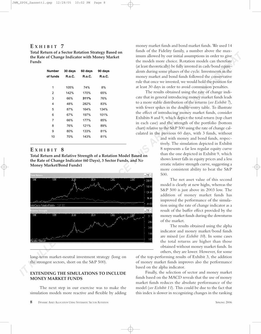
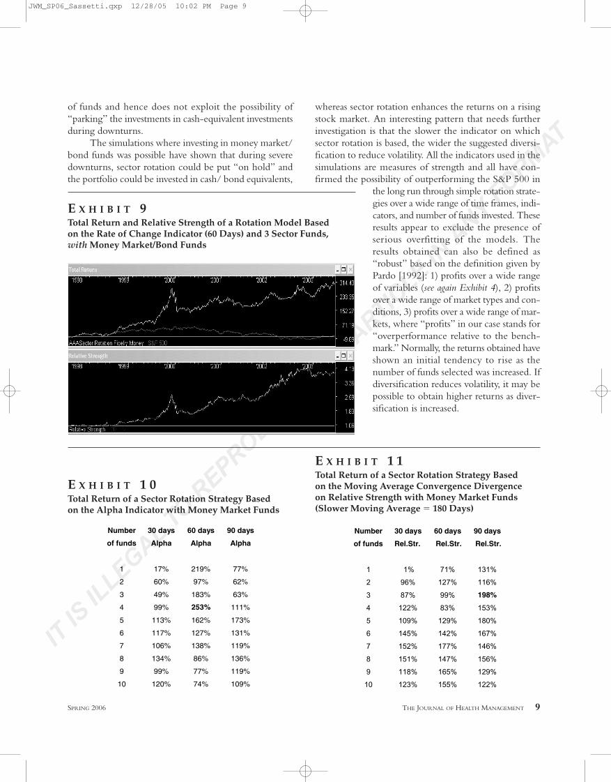
The results obtained using the rate of change indi-cate that in general introducing money market funds leadsto a more stable distribution of the returns (see Exhibit 7),with fewer spikes in the double-entry table. To illustratethe effect of introducing money market funds, considerExhibits 8 and 9, which depict the total return (top chartin each case) and the strength of the portfolio (bottomchart) relative to the S&P 500 using the rate of change cal-culated in the previous 60 days, with 3 funds, without

and with money and bond funds, respec-tively. The simulation depicted in Exhibit8 represents a far less regular equity curvethan the one depicted in Exhibit 9, whichshows lower falls in equity prices and a lesserratic relative strength curve, suggesting amore consistent ability to beat the S&P500.

The net asset value of this secondmodel is clearly at new highs, whereas theS&P 500 is just above its 2003 low. Theaddition of money market funds hasimproved the performance of the simula-tion using the rate of change indicator as aresult of the buffer effect provided by themoney market funds during the downturnsof the market.

The results obtained using the alphaindicator and money market/bond fundsare mixed (see Exhibit 10). In some casesthe total returns are higher than thoseobtained without money market funds. Inothers, they are lower. However, for some

of the top-performing results of Exhibit 3, the additionof money market funds improves also the performancebased on the alpha indicator.

Finally, the selection of sector and money marketfunds based on the MACD reveals that the use of moneymarket funds reduces the absolute performance of themodel (see Exhibit 11). This could be due to the fact thatthis index is slower in recognizing changes in the ranking



of funds R.o.C. R.o.C. R.o.C.

1 105% 74% 8%

2 142% 170% 65%

3 66% 311% 76%

4 48% 282% 83%

5 87% 164% 134%

6 67% 197% 101%

7 66% 177% 85%

8 76% 121% 89%

9 80% 133% 81%

10 70% 143% 81%

E X H I B I T 7Total Return of a Sector Rotation Strategy Based onthe Rate of Change Indicator with Money MarketFunds

E X H I B I T 8Total Return and Relative Strength of a Rotation Model Based onthe Rate of Change Indicator (60 Days), 3 Sector Funds, and NoMoney Market/Bond Funds1


IT IS

ILLEGAL T

O REPRODUCE T

HIS A

RTICLE IN

ANY F

ORMAT

whereas sector rotation enhances the returns on a risingstock market. An interesting pattern that needs furtherinvestigation is that the slower the indicator on whichsector rotation is based, the wider the suggested diversi-fication to reduce volatility. All the indicators used in thesimulations are measures of strength and all have con-firmed the possibility of outperforming the S&P 500 in

the long run through simple rotation strate-gies over a wide range of time frames, indi-cators, and number of funds invested. Theseresults appear to exclude the presence ofserious overfitting of the models. Theresults obtained can also be defined as“robust” based on the definition given byPardo [1992]: 1) profits over a wide rangeof variables (see again Exhibit 4), 2) profitsover a wide range of market types and con-ditions, 3) profits over a wide range of mar-kets, where “profits” in our case stands for“overperformance relative to the bench-mark.” Normally, the returns obtained haveshown an initial tendency to rise as thenumber of funds selected was increased. Ifdiversification reduces volatility, it may bepossible to obtain higher returns as diver-sification is increased.


E X H I B I T 9Total Return and Relative Strength of a Rotation Model Basedon the Rate of Change Indicator (60 Days) and 3 Sector Funds,with Money Market/Bond Funds


of funds Alpha Alpha Alpha

1 17% 219% 77%

2 60% 97% 62%

3 49% 183% 63%

4 99% 253% 111%

5 113% 162% 173%

6 117% 127% 131%

7 106% 138% 119%

8 134% 86% 136%

9 99% 77% 119%

10 120% 74% 109%

E X H I B I T 1 0Total Return of a Sector Rotation Strategy Basedon the Alpha Indicator with Money Market Funds



1 1% 71% 131%

2 96% 127% 116%

3 87% 99% 198%

4 122% 83% 153%

5 109% 129% 180%

6 145% 142% 167%

7 152% 177% 146%

8 151% 147% 156%

9 118% 165% 129%

10 123% 155% 122%

E X H I B I T 1 1Total Return of a Sector Rotation Strategy Basedon the Moving Average Convergence Divergenceon Relative Strength with Money Market Funds(Slower Moving Average � 180 Days)

of funds and hence does not exploit the possibility of“parking” the investments in cash-equivalent investmentsduring downturns.

The simulations where investing in money market/bond funds was possible have shown that during severedownturns, sector rotation could be put “on hold” andthe portfolio could be invested in cash/ bond equivalents,


IT IS

ILLEGAL T

O REPRODUCE T

HIS A

RTICLE IN

ANY F

ORMAT

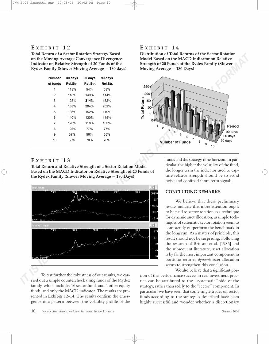
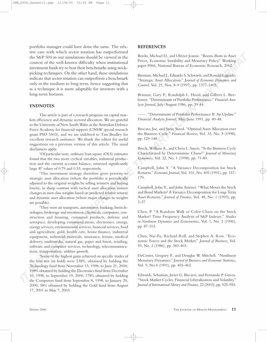
To test further the robustness of our results, we car-ried out a simple countercheck using funds of the Rydexfamily, which includes 16 sector funds and 4 other equityfunds, and only the MACD indicator. The results are pre-sented in Exhibits 12-14. The results confirm the emer-gence of a pattern between the volatility profile of the

funds and the strategy time horizon. In par-ticular, the higher the volatility of the fund,the longer term the indicator used to cap-ture relative strength should be to avoidnoise and confused short-term signals.

CONCLUDING REMARKS

We believe that these preliminaryresults indicate that more attention oughtto be paid to sector rotation as a techniquefor dynamic asset allocation, as simple tech-niques of systematic sector rotation seem toconsistently outperform the benchmark inthe long run. As a matter of principle, thisresult should not be surprising. Followingthe research of Brinson et al. [1986] andthe subsequent literature, asset allocationis by far the most important component inportfolio returns: dynamic asset allocationseems to strengthen this conclusion.

We also believe that a significant por-tion of this performance success in real investment prac-tice can be attributed to the “systematic” side of thestrategy, rather than solely to the “sector” component. Inparticular, we have seen that some single trades on sectorfunds according to the strategies described have beenhighly successful and wonder whether a discretionary




1 113% 54% 63%

2 118% 149% 114%

3 125% 214% 152%

4 133% 204% 209%

5 136% 152% 119%

6 140% 120% 115%

7 128% 110% 103%

8 103% 77% 77%

9 52% 56% 65%

10 56% 78% 73%

E X H I B I T 1 2Total Return of a Sector Rotation Strategy Basedon the Moving Average Convergence DivergenceIndicator on Relative Strength of 20 Funds of theRydex Family (Slower Moving Average � 180 days)

12

34

56

78

910

30 days60 days

90 days

0

50

100

150

200

250

To

tal R

etu

rnNumber of Funds

Period

E X H I B I T 1 4Distribution of Total Returns of the Sector RotationModel Based on the MACD Indicator on RelativeStrength of 20 Funds of the Rydex Family (SlowerMoving Average � 180 Days)

E X H I B I T 1 3Total Return and Relative Strength of a Sector Rotation ModelBased on the MACD Indicator on Relative Strength of 20 Funds ofthe Rydex Family (Slower Moving Average � 180 Days)


IT IS

ILLEGAL T

O REPRODUCE T

HIS A

RTICLE IN

ANY F

ORMAT

portfolio manager could have done the same. The rela-tive ease with which sector rotation has outperformedthe S&P 500 in our simulations should be viewed in thecontext of the well-known difficulty when institutionalinvestment funds try to beat their benchmarks using stock-picking techniques. On the other hand, these simulationsindicate that sector rotation can outperform a benchmarkonly in the medium to long term, hence suggesting thatas a technique it is more adaptable for investors with along-term horizon.

ENDNOTES

This article is part of a research program on capital mar-kets efficiency and dynamic sectoral allocation. We are gratefulto the University of New South Wales at the Australian DefenceForce Academy for financial support (UNSW special researchgrant PSO 5503), and we are indebted to Tim Bradley forexcellent research assistance. We thank the editor for usefulsuggestions on a previous version of this article. The usualdisclaimers apply.

1Of particular note, ordinary least square (OLS) estimatesfound that the two more cyclical variables, industrial produc-tion and the current account balance, returned significantlylarge R2 values of 0.79 and 0.53, respectively.

2This investment strategy therefore gives priority tostrategic asset allocation (where the portfolio is periodicallyadjusted to the original weights by selling winners and buyinglosers), in sharp contrast with tactical asset allocation (minorchanges in asset class weights based on predicted relative return)and dynamic asset allocation (where major changes in weightsare possible).

3They were air transports, automotive, banking, biotech-nologies, brokerage and investment, chemicals, computers, con-struction and housing, consumer products, defense andaerospace, developing communications, electronics, energy,energy services, environmental services, financial services, foodand agriculture, gold, health care, home finance, industrialequipment, industrial materials, insurance, leisure, medicaldelivery, multimedia, natural gas, paper and forest, retailing,software and computer services, technology, telecommunica-tions, transportation, utilities growth.

4Some of the highest gains achieved on specific trades ofthe best test (in bold) were 238%, obtained by holding theTechnology fund from November 13, 1998, to June 21, 2000;198% obtained by holding the Electronics fund from December10, 1998, to September 19, 2000; 178% obtained by holdingthe Computers fund from September 8, 1998, to January 20,2000; 58% obtained by holding the Gold fund from August17, 2001 to May 7, 2003.

REFERENCES

Bordo, Michael D., and Olivier Jeanne. “Boom-Busts in AssetPrices, Economic Instability and Monetary Policy.” Workingpaper 8966, National Bureau of Economic Research, 2002.

Brennan, Michael J., Eduardo S. Schwartz, and Ronald Lagnado.“Strategic Asset Allocation.” Journal of Economic Dynamics andControl, Vol. 21, Nos. 8-9 (1997), pp. 1377-1403.

Brinson, Gary P., Randolph L. Hood, and Gilbert L. Bee-bower. “Determinants of Portfolio Performance.” Financial Ana-lysts Journal, July/August 1986, pp. 39-44.

——. “Determinants of Portfolio Performance II: An Update.”Financial Analysts Journal, May/June 1991, pp. 40-48.

Brocato, Joe, and Steve Steed. “Optimal Asset Allocation overthe Business Cycle.” Financial Review, Vol. 33, No. 3 (1998),pp. 129-148.

Brock, William A., and Chera L. Sayers. “Is the Business CycleCharacterized by Deterministic Chaos?” Journal of MonetaryEconomics, Vol. 22, No. 1 (1998), pp. 71-80.

Campbell, John Y. “A Variance Decomposition for StockReturns.” Economic Journal, Vol. 101, No. 405 (1991), pp. 157-179.

Campbell, John Y., and John Ammer. “What Moves the Stockand Bond Markets? A Variance Decomposition for Long-TermAsset Returns.” Journal of Finance, Vol. 48, No. 1 (1993), pp.3-37.

Chen, P. “A Random Walk or Color Chaos on the StockMarket? Time Frequency Analysis of S&P Indexes.” Studiesin Nonlinear Dynamics and Econometrics, Vol. 1, No. 2 (1996),pp. 87-103.

Chen, Nai-Fu, Richard Roll, and Stephen A. Ross. “Eco-nomic Forces and the Stock Market.” Journal of Business, Vol.59, No. 3 (1986), pp. 383-403.

DeCoster, Gregory P., and Douglas W. Mitchell. “NonlinearMonetary Dynamics.” Journal of Business and Economic Statistics,Vol. 9, No.4 (1991), pp. 455-462.

Edwards, Sebastian, Javier G. Biscarri, and Fernando P. Gracia.“Stock Market Cycles, Financial Liberalization and Volatility.”Journal of International Money and Finance, 22 (2003), pp. 925-955.



IT IS

ILLEGAL T

O REPRODUCE T

HIS A

RTICLE IN

ANY F

ORMAT

Fama, Eugene, and Robert R. Bliss. “The Information in LongMaturity Forward Rates.” American Economic Review, Vol. 77,No. 4 (1987), pp. 680-692.

Fama, Eugene, and William G. Schwert. “Asset Returns andInflation.” Journal of Financial Economics, Vol. 5, No. 2 (1977),pp. 115-146.

Flavin, Thomas J., and Michael R. Wickens. “A Risk Man-agement Approach to Optimal Asset Allocation.” Workingpaper N85, NUI Maynooth, December 1998.

——. “Macroeconomic Influences on Optimal Asset Alloca-tion.” Review of Financial Economics, Vol. 12, No. 2 (2003),pp. 207-231.

Fowler, Stuart. “Asset Allocation: Too Important to Be Left toMoney Managers.” Professional Investor, February (1997).

Grauer, Robert R., Nils H. Hakansson, and Frederick C. Shen.“Industry Rotation in the US Stock Market: 1934–1986 Returnson Passive, Semi-Passive, and Active Strategies.” Journal of Bankingand Finance, Vol. 14, Nos. 2-3 (August 1990), pp. 513-535.

——. “Stein and CAPM Estimators of the Means in Asset Allo-cation.” International Review of Financial Analysis, Vol. 4, No. 1(1995), pp. 35-66.

Harloff, G.J. “Dynamic Asset Allocation: Beyond Buy andHold.” Technical Analysis of Stocks and Commodities Magazine,January 1998.

Harvey, Campbell R. “The World Price of Covariance Risk.”Journal of Finance, Vol. 46, No. 1 (1991), pp. 111-157.

Keraney, C., and K. Daly. “The Causes of Stock MarketVolatility in Australia.” Applied Financial Economics, 8 (1998),pp. 597-605.

King, M., S. Oscar, and B. Guo. “Passive Momentum AssetAllocation”, The Journal of Wealth Management, Winter 2002.

Moore, Geoffrey H. Business Cycles, Inflation and Forecasting,2nd ed. Cambridge, MA: Ballinger Publishing Co., 1983.

Officer, R.R. “The Variability of the Market Factor of theNew York Stock Exchange.” Journal of Business, Vol. 46, No. 3(1973), pp. 434-453.

Pardo, Robert. Design, Testing, and Optimization of TradingSystems. New York: Wiley, 1992.

Ramsey, James B., Chera L. Sayers, and Philip Rothman. “TheStatistical Properties of Dimension Calculations Using SmallData Sets: Some Economic Applications.” International EconomicReview, Vol. 31, No. 4 (1990), pp. 991-1020.

Ross, Stephen A., and Randall C. Zisler. “Risk and Return inReal Estate.” Journal of Real Estate Finance and Economics, Vol. 4,No. 2 (1991), pp. 175-190.

Sadorsky, Perry. “The Macroeconomic Determinants of Tech-nology Stock Price Volatility.” Review of Financial Economics,Vol. 12, No. 2 (2003), pp. 191-205.

Schwager, Jack D. The New Market Wizards. New York: HarperBusiness, 1992.

Schwert, G. William. “Indexes of United States Stock Pricesfrom 1802 to 1987.” Journal of Business, Vol. 63, No. 3 (1990),pp. 399-426.

——. “Why Does Stock Market Volatility Change over Time?”Journal of Finance, Vol. 44, No. 5 (1989), pp. 1115-1153.

Shiller, Robert J., John Y. Campbell, and Kermit L. Schoen-holtz. “Forward Rates and Future Policy, Interpreting the TermStructure of Interest Rates.” Brookings Papers on Economic Activity,1 (1983), pp. 173-217.

Stovall, Sam. Sector Investing. New York: McGraw Hill, 1996.

Zisler, Randall C. Managing Real Estate Portfolios: A DynamicProcess, 2nd ed. Boston, MA: Warren, Gorham and LaMontPublishing, 1990.

To order reprints of this article, please contact Dewey Palmieri [email protected] or 212-224-3675.



Dynamic Asset Allocation Using Systematic Sector Rotation

Documents