University of Windsor University of Windsor Scholarship at UWindsor Scholarship at UWindsor Electronic Theses and Dissertations Theses, Dissertations, and Major Papers 2004 Dynamic and static analyses of continuous curved composite Dynamic and static analyses of continuous curved composite multiple-box girder bridges. multiple-box girder bridges. Magdy Said Samaan University of Windsor Follow this and additional works at: https://scholar.uwindsor.ca/etd Recommended Citation Recommended Citation Samaan, Magdy Said, "Dynamic and static analyses of continuous curved composite multiple-box girder bridges." (2004). Electronic Theses and Dissertations. 1791. https://scholar.uwindsor.ca/etd/1791 This online database contains the full-text of PhD dissertations and Masters’ theses of University of Windsor students from 1954 forward. These documents are made available for personal study and research purposes only, in accordance with the Canadian Copyright Act and the Creative Commons license—CC BY-NC-ND (Attribution, Non-Commercial, No Derivative Works). Under this license, works must always be attributed to the copyright holder (original author), cannot be used for any commercial purposes, and may not be altered. Any other use would require the permission of the copyright holder. Students may inquire about withdrawing their dissertation and/or thesis from this database. For additional inquiries, please contact the repository administrator via email ([email protected]) or by telephone at 519-253-3000ext. 3208.

Welcome message from author
This document is posted to help you gain knowledge. Please leave a comment to let me know what you think about it! Share it to your friends and learn new things together.
Transcript
University of Windsor University of Windsor
Scholarship at UWindsor Scholarship at UWindsor
Electronic Theses and Dissertations Theses, Dissertations, and Major Papers
2004
Dynamic and static analyses of continuous curved composite Dynamic and static analyses of continuous curved composite
multiple-box girder bridges. multiple-box girder bridges.
Magdy Said Samaan University of Windsor
Follow this and additional works at: https://scholar.uwindsor.ca/etd
Recommended Citation Recommended Citation Samaan, Magdy Said, "Dynamic and static analyses of continuous curved composite multiple-box girder bridges." (2004). Electronic Theses and Dissertations. 1791. https://scholar.uwindsor.ca/etd/1791
This online database contains the full-text of PhD dissertations and Masters’ theses of University of Windsor students from 1954 forward. These documents are made available for personal study and research purposes only, in accordance with the Canadian Copyright Act and the Creative Commons license—CC BY-NC-ND (Attribution, Non-Commercial, No Derivative Works). Under this license, works must always be attributed to the copyright holder (original author), cannot be used for any commercial purposes, and may not be altered. Any other use would require the permission of the copyright holder. Students may inquire about withdrawing their dissertation and/or thesis from this database. For additional inquiries, please contact the repository administrator via email ([email protected]) or by telephone at 519-253-3000ext. 3208.
DYNAMIC AND STATIC ANALYSES OF CONTINUOUS CURVED COMPOSITE MULTIPLE-BOX GIRDER
BRIDGES
BY
MAGDY SAID SAMAAN
A DissertationSubmitted to the Faculty of Graduate Studies and Research through
the Department of Civil and Environmental Engineering in partial fulfillment of the requirements for the
degree of Doctor of Philosophy at the University of Windsor
Windsor, Ontario, Canada 2004
Reproduced with permission of the copyright owner. Further reproduction prohibited without permission.

1 ^ 1National Library of Canada
Acquisitions and Bibliographic Services
395 Wellington Street Ottawa ON K1A 0N4 Canada
Bibliotheque nationals du Canada
Acquisisitons et services bibliographiques
395, rue Wellington Ottawa ON K1A 0N4 Canada
Your file Votre reference ISBN: 0-612-92551-X Our file Notre reference ISBN: 0-612-92551-X
The author has granted a nonexclusive licence allowing the National Library of Canada to reproduce, loan, distribute or sell copies of this thesis in microform, paper or electronic formats.
The author retains ownership of the copyright in this thesis. Neither the thesis nor substantial extracts from it may be printed or otherwise reproduced without the author's permission.
L'auteur a accorde une licence non exclusive permettant a la Bibliotheque nationale du Canada de reproduire, preter, distribuer ou vendre des copies de cette these sous la forme de microfiche/film, de reproduction sur papier ou sur format electronique.
L'auteur conserve la propriete du droit d'auteur qui protege cette these. Ni la these ni des extraits substantiels de celle-ci ne doivent etre imprimes ou aturement reproduits sans son autorisation.
In compliance with the Canadian Privacy Act some supporting forms may have been removed from this dissertation.
Conformement a la loi canadienne sur la protection de la vie privee, quelques formulaires secondaires ont ete enleves de ce manuscrit.
While these forms may be included in the document page count, their removal does not represent any loss of content from the dissertation.
Bien que ces formulaires aient inclus dans la pagination, il n'y aura aucun contenu manquant.
CanadaReproduced with permission of the copyright owner. Further reproduction prohibited without permission.

Magdy Said SAMAAN©-------------------------------------------------- 2004
All Rights Reserved
Reproduced with permission of the copyright owner. Further reproduction prohibited without permission.

I hereby declare that I am the sole author of this document.
I authorize the University of Windsor to lend this document to other institutions or individuals for the purpose of scholarly research.
Magdy Said Samaan
I further authorize the University of Windsor to reproduce the document by photocopying or by other means, in total or part, at the request of other institutions or individuals for the purpose of scholarly research.
Magdy Said Samaan
IV
Reproduced with permission of the copyright owner. Further reproduction prohibited without permission.

THE UNIVERSITY OF WINDSOR requires the signatures of all persons using or photocopying this document.
Please sign below, and give address and date.
Reproduced with permission of the copyright owner. Further reproduction prohibited without permission.
Abstract
Horizontally curved concrete deck on multiple steel box girder bridges is a
structurally efficient, economic, and aesthetically pleasing method of supporting curved
roadway systems. Modem highway constractions are often in need of bridges with
horizontally curved alignments due to the tight geometry restrictions. Continuous curved
composite box girder bridges allow for the use of longer spans, thus reducing costs of the
substmcture.
Despite all inherent advantages of continuous curved composite box girder
bridges, they do pose challenging problems for engineers in calculating the load
distribution due to moving vehicles across the bridges. Curved bridges are subjected to
high torsional as well as flexural stresses. The interaction between the box girders is also
more complicated in curved bridges than that in straight bridges. North American codes
for bridges have recommended expressions for the load distribution factors only for
straight bridges and not for curved bridges. Impact factors proposed in these codes are
generally restricted also to straight bridges. In addition, simplifled formula to predict the
fundamental frequency of analyzing the bridges is not available. To assist engineers in
dealing with the complexities of continuous curved composite box girder bridges, a
reliable, accurate, and simple method is required to calculate the structure’s response
under self-weight and vehicular loading.
The refined three-dimensional finite-element analysis method is employed to
investigate the static and dynamic responses of the bridge. Two two-equal-span two-box
physical bridge models were constmcted in the laboratory. One of the bridge models was
vi
Reproduced with permission of the copyright owner. Further reproduction prohibited without permission.

straight in plan while the other was horizontally curved. The physical models were tested
under several static loading cases to better comprehend their elastic behaviour. Free-
vibration tests were also conducted to obtain the natural frequencies and the
corresponding mode shapes of the bridge models. Both models were loaded up to failure
to examine the collapse mechanism and its correlation with the finite element modeling.
Findings obtained from the two physical bridge models were compared to those predicted
by the analytical models. The agreement between the finite element model and the
experimental model made it possible to use the analytical models to conduct three
parametric studies on several bridges.
Vll
Reproduced with permission of the copyright owner. Further reproduction prohibited without permission.

TO MY FAMILY
V lll
Reproduced with permission of the copyright owner. Further reproduction prohibited without permission.

Acknowledgements
I would like to express my sincere thanks and deepest gratitude to GOD who
helped me and blessed me all the way of my study.
I would like to express my strongest appreciation to my co-advisor Dr. J.
Kermedy, University Distinguished Professor, for his patience, guidance, and support
throughout the course of this study. I would like to state my genuine thanks to my co
advisor Dr. K. Sennah, Associate Professor, for devoting his time and effort to make this
study a success.
I wish to thank Dr. Madugula, Dr. Hearn, Dr. Ghrib, and Dr. Budkowska for their
help and encouragement.
I wish to acknowledge the financial support provided by the Natural Sciences and
Engineering Research Council of Canada.
I am greatly indebted to my family, parents, and my wife for their strong
encouragement, support, understanding, and patience during the years of this study.
IX
Reproduced with permission of the copyright owner. Further reproduction prohibited without permission.
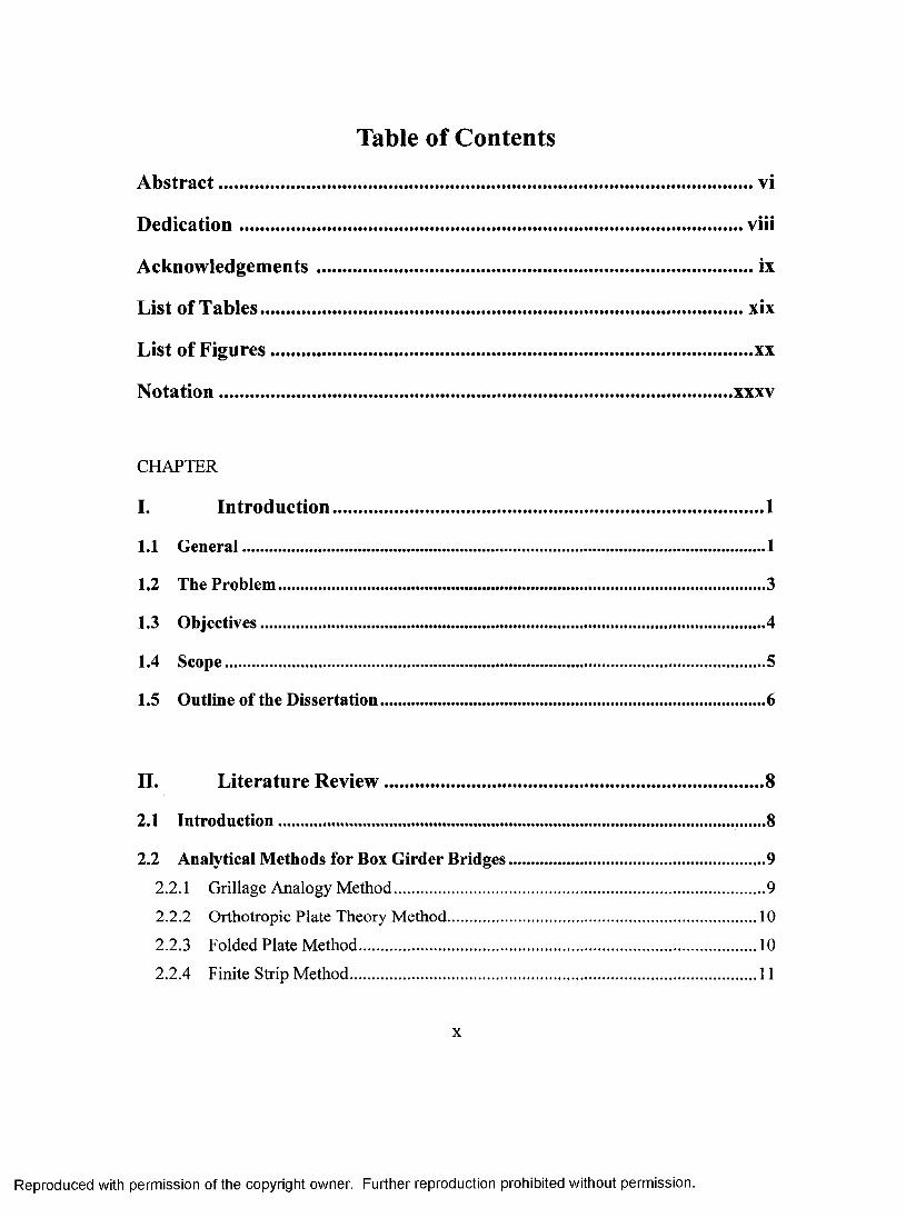
Table of Contents
Abstract................................................................................................................vi
Dedication......................................................................................................... viii
Acknowledgements............................................................................................ix
List of Tables..................................................................................................... xix
List of Figures.................................................................................................... xx
Notation...........................................................................................................xxxv
CHAPTER
I. Introduction...........................................................................................1
1.1 General............................................................................................................................ 1
1.2 The Problem................................................................................................................... 3
1.3 Objectives........................................................................................................................4
1.4 Scope................................................................................................................................ 5
1.5 Outline of the Dissertation........................................................................................... 6
II. Literature Review ................................................................................8
2.1 Introduction.............................................................. 8
2.2 Analytical Methods for Box Girder Bridges.............................................................9
2.2.1 Grillage Analogy Method.......................................................................................9
2.2.2 Orthotropic Plate Theory Method.........................................................................10
2.2.3 Folded Plate Method..............................................................................................10
2.2.4 Finite Strip Method................................................................................................11
X
Reproduced with permission of the copyright owner. Further reproduction prohibited without permission.
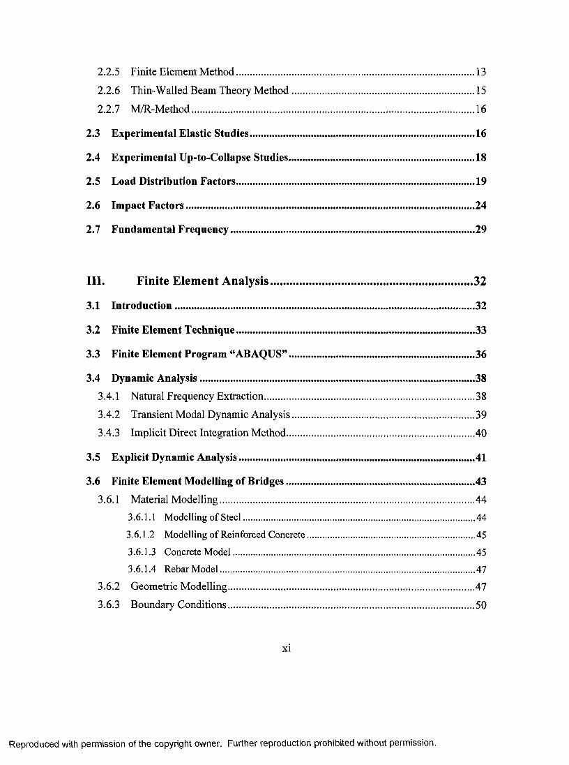
2.2.5 Finite Element Method......................................................................................... 13
2.2.6 Thin-Walled Beam Theory M ethod.................................................................... 15
2.2.7 M/R-Method.......................................................................................................... 16
2.3 Experimental Elastic Studies......................................................................................16
2.4 Experimental Up-to-CoIIapse Studies....................................................................... 18
2.5 Load Distribution Factors........................................................................................... 19
2.6 Impact Factors..............................................................................................................24
2.7 Fundamental Frequency.............................................................................................29
III. Finite Element Analysis....................................................................32
3.1 Introduction..................................................................................................................32
3.2 Finite Element Technique...........................................................................................33
3.3 Finite Element Program “ABAQUS” .......................................................................36
3.4 Dynamic Analysis........................................................................................................ 38
3.4.1 Natural Frequency Extraction.............................................................................. 38
3.4.2 Transient Modal Dynamic Analysis....................................................................39
3.4.3 Implicit Direct Integration Method...................................................................... 40
3.5 Explicit Dynamic Analysis..........................................................................................41
3.6 Finite Element Modelling of Bridges........................................................................43
3.6.1 Material Modelling.................................................................................................. 443.6.1.1 Modelling of Steel........................................................................................44
3.6.1.2 Modelling of Reinforced Concrete................................................................453.6.1.3 Concrete Model............................................................................................453.6.1.4 Rebar Model................................................................................................ 47
3.6.2 Geometric Modelling............................................................................................ 47
3.6.3 Boundary Conditions............................................................................................ 50
XI
Reproduced with permission of the copyright owner. Further reproduction prohibited without permission.
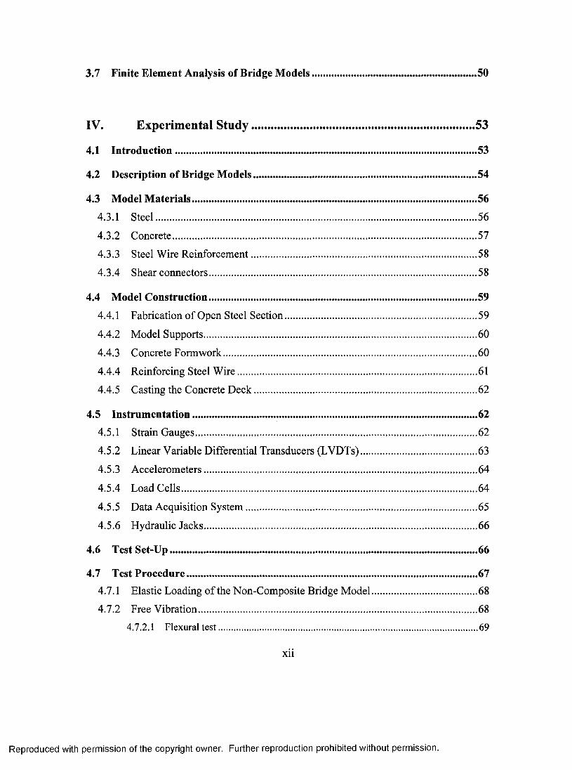
3.7 Finite Element Analysis of Bridge Models..............................................................50
IV. Experimental Study........................................................................... 53
4.1 Introduetion................................................................................................................. 53
4.2 Description of Bridge Models....................................................................................54
4.3 Model Materials...........................................................................................................56
4.3.1 Steel......................................................................................................................... 56
4.3.2 Conerete.................................................................................................................. 57
4.3.3 Steel Wire Reinforeement.....................................................................................58
4.3.4 Shear eonneetors..................................................................................................... 58
4.4 Model Construction.....................................................................................................59
4.4.1 Fabrieation of Open Steel Section........................................................................ 59
4.4.2 Model Supports....................................................................................................... 60
4.4.3 Concrete Form work............................................................................................... 60
4.4.4 Reinforcing Steel W ire.......................................................................................... 61
4.4.5 Casting the Concrete Deck.................................................................................... 62
4.5 Instrumentation........................................................................................................... 62
4.5.1 Strain Gauges...........................................................................................................62
4.5.2 Linear Variable Differential Transducers (LYDTs)............................................ 63
4.5.3 Accelerometers.......................................................................................................64
4.5.4 Load Cells............................................................................................................... 64
4.5.5 Data Acquisition System.......................................................................................65
4.5.6 Hydraulic Jacks.......................................................................................................66
4.6 Test Set-Up................................................................................................................... 66
4.7 T est Procedure............................................................................................................. 674.7.1 Elastic Loading of the Non-Composite Bridge Model..........................................68
4.7.2 Free Vibration.........................................................................................................68
4.7.2.1 Flexural test..................................................................................................69
xii
Reproduced with permission of the copyright owner. Further reproduction prohibited without permission.

4.7.2.2 Torsion test.................................................................................................. 70
4.7.3 Elastic Loading the Composite Bridge Models................................................... 70
4.7.4 Loading of Bridge Models Up-to-Collapse..........................................................73
V. Model Validation...............................................................................74
5.1 Introduction................................................................................................................. 74
5.2 Elastic Response of Non-Composite Straight Bridge Model................................75
5.2.1 Loading Case 1 .....................................................................................................75
5.2.2 Loading Case 2 .....................................................................................................76
5.2.3 Loading Case 3 .....................................................................................................77
5.2.4 Loading Case 4 .....................................................................................................78
5.2.5 Loading Case 5 .....................................................................................................79
5.3 Elastic Response of Non-Composite Curved Bridge Model ........................ 80
5.3.1 Loading Case 1 ..................................................................................................... 80
5.3.2 Loading Case 2 ..................................................................................................... 81
5.3.3 Loading Case 3 ..................................................................................................... 82
5.3.4 Loading Case 4 ..................................................................................................... 83
5.3.5 Loading Case 5 ..................................................................................................... 84
5.4 Elastic Response of Composite Straight Bridge Model......................................... 84
5.4.1 Loading Case 1 ..................................................................................................... 84
5.4.2 Loading Case 2 ..................................................................................................... 85
5.4.3 Loading Case 3 ..................................................................................................... 86
5.4.4 Loading Case 4 ..................................................................................................... 87
5.5 Elastic Response of Curved Composite Bridge Model.......................................... 88
5.5.1 Loading Case 1 ..................................................................................................... 88
5.5.2 Loading Case 2 ..................................................................................................... 89
5.5.3 Loading Case 3 .....................................................................................................90
5.5.4 Loading Case 4 .....................................................................................................91
Xlll
Reproduced with permission of the copyright owner. Further reproduction prohibited without permission.
5.5.5 Loading Case 5 ...................................................................................................... 92
5.5.6 Loading Case 6 ......................................................................................................92
5.6 Dynamic Characteristics of the Composite Bridge Model...................................94
5.7 Nonlinear Response of the Composite bridge model............................................ 96
5.8 Discrepancies between the Experimental and Theoretical Results......................... 101
5.9 Summary.................................................................................................................... 102
VI. Parametric Studies..........................................................................105
6.1 Introduction...............................................................................................................105
6.2 Description of Bridges Used in the Parametric Studies..................................... 106
6.3 Loading Conditions.................................................................................................. 110
6.3.1 Dead Load.............................................................................................................110
6.3.2 Live Load..............................................................................................................110
6.4 Parametric Study for Load Distribution Factors................................................112
6.4.1 AASHTO Live Loading......................................................................................114
6.4.2 Dead Load.............................................................................................................118
6.5 Parametric Study for Impact Factors....................................................................119
6.6 Parametric Study for the Fundamental Frequency............................................120
VII. Load Distribution Factors............................................................. 121
7.1 Introduction...............................................................................................................121
7.2 Distribution Factors for Tensile Stress..................................................................1227.2.1 Effect of Span Length..........................................................................................122
7.2.2 Effect of Number of Lanes..................................................................................122
7.2.3 Effect of Number of Boxes..................................................................................123
xiv
Reproduced with permission of the copyright owner. Further reproduction prohibited without permission.

7.2.4 Effect of Span-to-Radius of Curvature Ratio.................................................... 124
7.3 Distribution Factors for Compressive Stress........................................................124
7.3.1 Effect of Span Length.......................................................................................... 124
7.3.2 EffectofNumber of Lanes.................................................................................. 125
7.3.3 Effect of Number of Boxes................................................................................. 125
7.3.4 Effect of Span-to-Radius of Curvature Ratio....................................................126
7.4 Distribution Factors for Deflection.........................................................................126
7.4.1 Effect of Span Length..........................................................................................126
7.4.2 Effect of Number of Lanes................................................................................. 127
7.4.3 Effect of Number of Boxes................................................................................. 127
7.4.4 Effect of Span-to-Radius of Curvature Ratio....................................................128
7.5 Distribution Factors for S hear................................................................................128
7.5.1 Effect of Span Length.......................................................................................... 128
7.5.2 Effect of Number of Lanes................................................................................129
7.5.3 Effect of Number of Boxes................................................................................ 129
7.5.4 Effect of Span-to-Radius of Curvature Ratio.....................................................130
7.6 Distribution Factors for Exterior Support Reaction...........................................130
7.6.1 Effect of Span Length.......................................................................................... 130
7.6.2 Effect of Number of Lanes................................................................................ 131
7.6.3 Effect of Number of Boxes................................................................................ 131
7.7.1 Effect of Span-to-Radius of Curvature Ratio....................................................132
7.7 Distribution Factors for Interior Support Reaction............................................ 132
7.7.1 Effect of Span Length..........................................................................................132
7.7.2 Effect of Number of Lanes................................................................................ 133
7.7.3 Effect of Number of Boxes................................................................................ 133
7.7.4 Effect of Span-to-Radius of Curvature Ratio.....................................................133
7.8 Distribution Factors for Minimum Reaction........................................................134
7.8.1 Effect of Span Length.......................................................................................... 134
7.8.2 Effect of Number of Lanes................................................................................ 135
XV
Reproduced with permission of the copyright owner. Further reproduction prohibited without permission.
7.8.3 Effect of Number of Boxes............................................................... 135
7.8.4 Effect of Span-to-Radius of Curvature Ratio.....................................................136
7.9 Empirical Formulas For Load Distribution Factors...........................................136
7.10 Effect of Number of Spans......................................................................................140
7.11 Effeet of Inclined Webs...........................................................................................142
7.12 Effect of Span-to-Depth Ratio............................................................................... 143
7.13 Effect of Cross Bracing...........................................................................................145
7.14 Effect of Different Types of Live Loading........................................................... 147
7.15 Illustrative Design Example....................................................................................149
7.16 Summary................................................................................................................... 152
VIII. Impact Factors.................................................................................. 154
8.1 Introduction.............................................................................................................. 154
8.2 Vehicle Idealization................................................................................................. 155
8.3 Vehicle Loading Positions....................................................................................... 157
8.4 Vehicle Speed............................................................................................................158
8.5 Mode Superposition versus Direct Integration Method................................... 160
8.6 Stability and Accuracy............................................................................................ 162
8.7 Damping Effect.........................................................................................................164
8.8 Dynamic Impact Factor.......................... ......165
8.9 Parametric Study......................................................................................................1668.9.1 Effect of Number of Lanes................................................................................. 1678.9.2 Effect of Number of Boxes................................................................................. 167
8.9.3 Effect of Span Length......................................................................................... 168
8.9.4 Effect of Span-to-Radius of Curvature Ratio....................................................168
xvi
Reproduced with permission of the copyright owner. Further reproduction prohibited without permission.
8.10 Expressions for Impact Factor................................................................................169
8.10.1 Impact Factor as a Fimction in Fundamental Frequency................................. 170
8.10.2 Impact Factor as a Function in Bridge Span Length....................................... 172
8.10.3 Impact Factor as a Function in Span-to-Radius of Curvature Ratio............... 174
8.11 Summary................................................................................................................... 175
IX. Fundamental Frequency............................................................... 178
9.1 Introduction..............................................................................................................178
9.2 Effect of Span Length..............................................................................................179
9.3 Effect of Number of Lanes........................................................................................180
9.4 Effect of Number of Boxes........................................................................................180
9.5 Effect of Span-to-Radius of Curvature Ratio..................................................... 181
9.6 Empirical Expressions for Fundamental Frequency...........................................182
9.7 Comparison with Flexural Beam Theory.............................................................. 183
9.8 Effect of Span-to-Depth ratio.................................................................................184
9.9 Effect of End-Diaphragm Thickness..................................................................... 185
9.10 Effect of Cross Bracing........................................................................................... 186
9.11 Effect of Number of Spans......................................................................................186
9.12 Forced-Vibration Analysis......................................................................................187
9.12.1 Effect of Vehicle Speed....................................................................................... 187
9.12.2 Effect of Curvature R atio .................................................................................... 188
9.12.3 Effect of End-Diaphragm Thickness.................................................................. 188
9.12.4 Effect of Number of Cross Braeings.................................................................. 189
9.13 Summary................................................................................................................... 189
xvii
Reproduced with permission of the copyright owner. Further reproduction prohibited without permission.

X. Summary and Conclusions............................................................192
10.1 Summary.....................................................................................................................192
10.2 Conclusions..................................................................................................................194
10.3 Recommendation for Further Research......................................... 196
References..........................................................................................................197
Tables .............................................................................................................216
Figures ......................................................................... 223
Appendix A ....................................................................................................... 444
Appendix B ....................................................................................................... 449
Vita Auctoris.................................................................................................... 454
X V lll
Reproduced with permission of the copyright owner. Further reproduction prohibited without permission.

List of Tables
TABLE
4.1 Average properties of the eoncrete cylinders for the bridge models........................216
5.1 Natural frequencies and mode shape of tested bridge models..................................216
5.2 Fundamental frequency obtained from the experimental tests.................................217
6.1 Geometries of bridges used in parametrie study for load distribution factor 218
6.2 Geometries of bridges used in parametric study for impact factor and fundamental frequency..................................................................................................................... 219
6.3 Vehicle speed used in parametric study for impact factor........................................ 220
7.1 Comparison between the results obtained from finite element analysis and theproposed method for different codes for load distribution factor............................221
9.1 Comparison between the finite-element results and proposed equations forfundamental frequency............................................................................................... 222
XIX
Reproduced with permission of the copyright owner. Further reproduction prohibited without permission.
List of Figures
FIGURE
1.1 Various box girder cross-sections............................................................................. 223
1.2 View of continuous curved composite twin box-girder bridge .............................. 224
1.3 Box girder bridge under construction (US290/IH 35 interchange, Direct connector Z) .................................................................................................................................224
1.4 Typical twin-box girder bridge cross section .......................................................... 225
3.1 Stress-strain relationship for steel adopted in ABAQUS model ............................226
3.2 Tension stiffening model in reinforced concrete..................................................... 226
3.3 Uniaxial stress-strain relationship for plain concrete ............................................. 227
3.4 Concrete failure surfaces in plane stress ................................................................. 227
3.5 Finite element discretization of cross-section of the bridge models.......................228
3.6 Shell element “S4R” used for plate modelling........................................................ 229
3.7 Beam element “B3IH” for beam in space................................................................230
3.8 Boundary condition of the bridges used in the parametric studies......................... 231
3.9 Typical finite element mesh for: a) the non-composite bridge model; and b) the composite bridge m odel............................................................................................. 232
4.1 Plan for the experimental straight bridge model .....................................................233
4.2 Plan for the expereimental curved bridge m odel.....................................................234
4.3 Cross-sectional details of the bridge models ........................................................... 235
4.4 Tension test set-up for steel reinforcement specimen used in the bridge models ..236
4.5 True stress-true strain relationship for structural steel plate...................................236
4.6 View of a tested concrete cylinder after failure.......................................................237
XX
Reproduced with permission of the copyright owner. Further reproduction prohibited without permission.

4.7 Stress-strain relationship for concrete cylinders of the curved bridge model ...237
4.8 Stress-strain relationship for the reinforcing s tee l...................................................238
4.9 True stress-true strain relationship for steel shear connectors................................ 238
4.10 View of shear connectors welded to the top flange.................................................239
4.11 View of straight bridge model during fabrication ................................................... 239
4.12 View of the formwork for the curved bridge model.................................................240
4.13 View of the formwork and reinforcing steel bars for the straight bridge model ....240
4.14 View of the formwork and reinforcing steel bars for the curved bridge model ....241
4.15 View of the curved bridge model along with the concrete cylinders during curing ... ...................................................................................................................................... 241
4.16 View of the strain gauges installed along the bottom flange width at the mid-span section...........................................................................................................................242
4.17 Locations of strain gauges on the longitudinal direction of the bridge m odels... 243
4.18 View of the LVDTs in the first span of the bridge m odel.......................................244
4.19 Locations of LVDTs in the cross section of the bridge m odel............................... 245
4.20 View of the accelerometers in the second span of the bridge model .....................246
4.21 Locations of accelerometers in the cross section of the bridge model ....................247
4.22 View of the load eells at the exterior support...........................................................248
4.23 Locations of load cells at support lines of the bridge m odel.................................. 249
4.24 Details of bearings......................................................................................................250
4.25 Data acquisition system cormected to the straight bridge m odel............................251
4.26 Test set-up for the straight bridge m odel..................................................................251
4.27 View of Loading Case 1 applied to the non-composite straight bridge model ....252
4.28 View of the flexural vibration test for straight bridge model................................. 253
4.29 View of the torsional vibration test for curved bridge m odel................................ 254
XXI
Reproduced with permission of the copyright owner. Further reproduction prohibited without permission.

4.30 View of straight bridge model imder Loading Case 1 ............................................255
4.31 View of straight bridge model under Loading Case 2 ........................................... 255
4.32 View of straight bridge model under Loading Case 3 ........................................... 256
4.33 View of straight bridge model under Loading Case 4 ............................................256
4.34 View of curved bridge model under Loading Case 1 .............................................. 257
4.35 View of curved bridge model under Loading Case 2 ..............................................257
4.36 View of curved bridge model under Loading Case 3 ..............................................258
4.37 View of curved bridge model under Loading Case 4 ............................................. 258
4.38 View of curved bridge model under Loading Case 5 ..............................................259
4.39 View of curved bridge model under Loading Case 6 ..............................................259
5.1 Cases of loading for non-composite straight bridge m odel................................... 260
5.2 Deflections of the non-composite straight bridge model due to Loading Case 1 ..261
5.3 Longitudinal strains of the non-composite straight bridge model due to Loading C asel ..........................................................................................................................262
5.4 Reactions for the non-composite straight bridge model due to Loading Case 1 ...263
5.5 Deflections of the non-composite straight bridge model due to Loading Case 2 ..264
5.6 Longitudinal strain distributions of the non-composite straight bridge model due to loading case 2 .............................................................................................................265
5.7 Reactions for the non-composite straight bridge model due to Loading Case 2 ...266
5.8 Deflections of the non-composite straight bridge model due to Loading Case 3 ..267
5.9 Longitudinal strains of the non-composite straight bridge model due to Loading Case 3 ..........................................................................................................................268
5.10 Reactions for the non-composite straight bridge model due to Loading Case 3 ...269
5.11 Deflections of the non-composite straight bridge model due to Loading Case 4 ..270
5.12 Longitudinal strains of the non-composite straight bridge model due to Loading Case 4 ..........................................................................................................................271
xxii
Reproduced with permission of the copyright owner. Further reproduction prohibited without permission.
5.13 Reactions for the non-composite straight bridge model due to Loading Case 4 ...272
5.14 Deflections of the non-composite straight bridge model due to Loading Case 5 ..273
5.15 Longitudinal strains of the non-composite straight bridge model due to Loading Case 5 ..........................................................................................................................274
5.16 Reactions for the non-composite straight bridge model due to Loading Case 5 ...275
5.17 Cases of loading for the non-composite curved bridge model ............................... 276
5.18 Deflections of the non-composite curved bridge model due to Loading Case 1 ...277
5.19 Longitudinal strains of the non-composite curved bridge model due to Loading C asel ..........................................................................................................................278
5.20 Reactions for the non-composite curved bridge model due to Loading Case 1 ....279
5.21 Deflections of the non-composite curved bridge model due to Loading Case 2 ...280
5.22 Longitudinal strains of the non-composite curved bridge model due to Loading Case 2 ..........................................................................................................................281
5.23 Reactions for the non-composite curved bridge model due to Loading Case 2 ....282
5.24 Deflections of the non-composite curved bridge model due to Loading Case 3 ...283
5.25 Longitudinal strains of the non-composite curved bridge model due to Loading Case 3 ..........................................................................................................................284
5.26 Reactions for the non-composite curved bridge model due to Loading Case 3 ....285
5.27 Deflections of the non-composite curved bridge model due to Loading Case 4 ...286
5.28 Longitudinal strains of the non-composite curved bridge model due to Loading Case 4 ..........................................................................................................................287
5.29 Reactions for the non-composite curved bridge model due to Loading Case 4 ....288
5.30 Deflections of the non-composite curved bridge model due to Loading Case 5 ...289
5.31 Longitudinal strains of the non-composite curved bridge model due to Loading Case 5 ..........................................................................................................................290
5.32 Reactions for the non-composite curved bridge model due to Loading Case 5 ....291
X X lll
Reproduced with permission of the copyright owner. Further reproduction prohibited without permission.

5.33 Cases of loading for the composite straight bridge model .................................... 292
5.34 Deflections of the composite straight bridge model due to Loading Case 1 ........293
5.35 Longitudinal strains of the composite straight bridge model due to Loading Case 1 294
5.36 Reactions for the composite straight bridge model due to Loading Case 1 .........295
5.37 Deflections of the composite straight bridge model due to Loading Case 2 ........296
5.38 Longitudinal strains of the composite straight bridge model due to Loading Case 2 297
5.39 Reactions for the composite straight bridge model due to Loading Case 2 .........298
5.40 Deflections of the composite straight bridge model due to Loading Case 3 ........299
5.41 Longitudinal strains of the composite straight bridge model due to Loading Case 3 300
5.42 Reactions for the composite straight bridge model due to Loading Case 3 .........301
5.43 Deflections of the composite straight bridge model due to Loading Case 4 ........302
5.44 Longitudinal strains of the composite straight bridge model due to Loading Case 4 303
5.45 Reactions for the composite straight bridge model due to Loading Case 4 .........304
5.46 Cases of loading for the composite curved bridge model ..................................... 305
5.47 Deflections of the composite curved bridge model due to Loading Case 1 .........306
5.48 Longitudinal strains of the composite curved bridge model due to Loading Case 1 ...................................................................................................................................... 307
5.49 Reactions for the composite curved bridge model due to Loading Case 1 ..........308
5.50 Deflections of the composite curved bridge model due to Loading Case 2 .........309
5.51 Longitudinal strains of the composite curved bridge model due to Loading Case 2 ...................................................................................................................................... 310
5.52 Reactions for the composite curved bridge model due to Loading Case 2 .......... 311
XXIV
Reproduced with permission of the copyright owner. Further reproduction prohibited without permission.
5.53 Deflections of the composite curved bridge model due to Loading Case 3 ..........312
5.54 Longitudinal strains of the composite curved bridge model due to Loading Case 3 ...................................................................................................................................... 313
5.55 Reactions for the composite curved bridge model due to Loading Case 3 ...........314
5.56 Deflections of the composite curved bridge model due to Loading Case 4 ......... 315
5.57 Longitudinal strains of the composite curved bridge model due to Loading Case 4 ...................................................................................................................................... 316
5.58 Reactions for the composite curved bridge model due to Loading Case 4 ...........317
5.59 Deflections of the composite curved bridge model due to Loading Case 5 ......... 318
5.60 Longitudinal strains of the composite curved bridge model due to Loading Case 5 ...................................................................................................................................... 319
5.61 Reactions for the composite curved bridge model due to Loading Case 5 ...........320
5.62 Deflections of the composite curved bridge model due to Loading Case 6 ..........321
5.63 Longitudinal strains of the composite curved bridge model due to Loading Case 6 ...................................................................................................................................... 322
5.64 Reactions for the composite curved bridge model due to Loading Case 6 ........... 323
5.65 Typical acceleration-time history of the straight bridge m odel.............................324
5.66 Typical displacement-time history of the straight bridge m odel........................... 324
5.67 Typical acceleration-time history of the curved bridge m odel.............................. 325
5.68 Typical displacement-time history of the curved bridge m odel............................ 325
5.69 Experimental acceleration frequency response of the straight bridge model in the flexural t e s t ................................................................................................................. 326
5.70 Experimental acceleration frequency response of the straight bridge model in the torsional te s t ................................................................................................................ 326
5.71 Experimental acceleration frequency response of the curved bridge model in the flexural test.................................................................................................................. 327
XXV
Reproduced with permission of the copyright owner. Further reproduction prohibited without permission.
5.72 Experimental acceleration frequency response of the curved bridge model in the torsional te s t ................................................................................................................ 327
5.73 First and second mode shapes obtained analytically for the bridge m odels.......... 328
5.74 First and second mode shapes obtained experimentally for the bridge models ....329
5.75 Load-deflection relationship for the straight bridge model at mid-span 1 ............ 330
5.76 Load-strain relationship of the concrete deck for the straight bridge model at midspan 1 ...........................................................................................................................330
5.77 Load-strain relationship of the bottom flange for the straight bridge model at midspan 1 ...........................................................................................................................331
5.78 Load-strain relationship at the top of the web for the straight bridge model at midspan 1 ...........................................................................................................................331
5.79 Load-strain relationship at the bottom of the weh for the straight bridge model at mid-span 1 .................................................................................................................. 332
5.80 Load-deflection relationship for the curved bridge model at mid-span 1 ............. 332
5.81 Load-deflection relationship for the curved bridge model at mid-span 1 .............. 333
5.82 Load-strain relationship of the concrete deck for the curved bridge model at midspan 1............................................................................................................................333
5.83 Load-strain relationship of the concrete deck for the curved bridge model at midspan 1............................................................................................................................334
5.84 Load-strain relationship of the bottom flange for the curved bridge model at midspan 1............................................................................................................................334
5.85 Load-strain relationship of the bottom flange for the curved bridge model at midspan 1............................................................................................................................335
5.86 Load-strain relationship at the top of the web for the curved bridge model at midspan 1 ...........................................................................................................................335
5.87 Load-strain relationship at the bottom of the weh for the curved bridge model at mid-span 1 .................................................................................................................. 336
5.88 Load-strain relationship at the top of the web for the curved bridge model at midspan 1 ...........................................................................................................................336
XXVI
Reproduced with permission of the copyright owner. Further reproduction prohibited without permission.
5.89 Load-strain relationship at the bottom of the web for the curved bridge model at mid-span 1 .................................................................................................................. 337
5.90 View of the deflected shape of the straight bridge model at failure........................338
5.91 View of the deflected shape of the curved bridge model at failure............... 338
5.92 Crack pattern of the concrete deck in the straight bridge model at failure....339
5.93 Crack pattern of the concrete deck in the curved bridge model at failure............. 339
5.94 Deformation of the bottom flange in the straight bridge model at failure.............. 340
5.95 Deformation of the bottom flange in the curved bridge model at failure............... 340
6.1 Symbols used for cross-section of four-box girder bridge........................................341
6.2 Cross-section configurations used in the parametric studies................................... 342
6.3 Effect of bottom flange thickness on distribution factor for tensile stress.....343
6.4 Effect of web thickness on distribution factor for tensile stress......................343
6.5 Standard truck and lane loads according to AASHTO Standard Specifications ...344
6.6 AASHTO truck loading cases in the transverse direction of the bridges............... 345
6.7 AASHTO truck loading cases considered in the parametric study for impact factor ...................................................................................................................................... 346
6.8 Idealized four-box bridge ........................................................................................... 347
6.9 AASHTO truck loading cases in the longitudinal direction of the bridges 348
6.10 Typical mode shapes for two-box girder bridge...................................................... 349
6.11 Typical mode shapes of two-equal-span continuous bridges ................................. 350
7.1 Effect of bridge span length on distribution factor for tensile stress for bridges dueto: a) AASHTO live load; and b) dead load .............................................................351
7.2 Effect of number of lanes on distribution factor for tensile stress for bridges due to:a) AASHTO live load; and b) dead load...................................................................352
7.3 Effect of number of boxes on distribution factor for tensile stress for bridges due to:a) AASHTO live load; and b) dead load...................................................................353
xxvii
Reproduced with permission of the copyright owner. Further reproduction prohibited without permission.

7.4 Effect of bridge curvature on distribution factor for tensile stress for bridges due to: a) AASHTO live load; and b) dead load...................................................................354
7.5 Effect of bridge span length on distribution factor for compressive stress for bridges due to: a) AASHTO live load; and b) dead load...................................................... 355
7.6 Effect of number of lanes on distribution factor for compressive stress for bridges due to: a) AASHTO live load; and b) dead load...................................................... 356
7.7 Effect of number of boxes on distribution factor for compressive stress for bridges due to: a) AASHTO live load; and b) dead load...................................................... 357
7.8 Effect of bridge curvature on distribution factor for compressive stress for bridges due to: a) AASHTO live load; and b) dead load...................................................... 358
7.9 Effect of bridge span length on distribution factor for deflection for bridges due to: a) AASHTO live load; and b) dead load...................................................................359
7.10 Effect of number of lanes on distribution factor for deflection for bridges due to: a)AASHTO live load; and b) dead load....................................................................... 360
7.11 Effect of number of boxes on distribution factor for deflection for bridges due to: a) AASHTO live load; and b) dead load....................................................................... 361
7.12 Effect of bridge curvature on distribution factor for deflection for bridges due to: a) AASHTO live load; and b) dead load ....................................................................... 362
7.13 Effect of bridge span length on distribution factor for shear force for bridges due to: a) AASHTO live load; and b) dead load...................................................................363
7.14 Effect of number of lanes on distribution factor for shear force for bridges due to: a)AASHTO live load; and b) dead load....................................................................... 364
7.15 Effect of number of boxes on distribution factor for shear force for bridges due to: a) AASHTO live load; and b) dead load...................................................................365
7.16 Effect of bridge curvature on distribution factor for shear force for bridges due to: a) AASHTO live load; and b) dead load...................................................................366
7.17 Effect of bridge span length on distribution factor for exterior support reaction for bridges due to: a) AASHTO live load; and b) dead load..........................................367
7.18 Effect of number of lanes on distribution factor for exterior support reaction for bridges due to: a) AASHTO live load; and b) dead load..........................................368
XXVlll
Reproduced with permission of the copyright owner. Further reproduction prohibited without permission.

7.19 Effect of number of boxes on distribution factor for exterior support reaction for bridges due to: a) AASHTO live load; and b) dead load..........................................369
7.20 Effect of bridge curvature on distribution factor for exterior support reaction for bridges due to: a) AASHTO live load; and b) dead load..........................................370
7.21 Effect of bridge span length on distribution factor for interior support reaction for bridges due to: a) AASHTO live load; and b) dead load..........................................371
7.22 Effect of number of lanes on distribution factor for interior support reaction for bridges due to: a) AASHTO live load; and b) dead load..........................................372
7.23 Effect of number of boxes on distribution factor for interior support reaction for bridges due to: a) AASHTO live load; and b) dead load..........................................373
7.24 Effect of bridge curvature on distribution factor for interior support reaction for bridges due to: a) AASHTO live load; and b) dead load..........................................374
7.25 Effect of bridge span length on distribution factor for minimum reaction for bridges due to: a) AASHTO live load; and b) dead load...................................................... 375
7.26 Effect of number of lanes on distribution factor for minimum reaction for bridges due to: a) AASHTO live load; and b) dead load...................................................... 376
7.27 Effect of number of boxes on distribution factor for minimum reaction for bridges due to: a) AASHTO live load; and b) dead load...................................................... 377
7.28 Effect of bridge curvature on distribution factor for minimum reaction for bridges due to: a) AASHTO live load; and b) dead load...................................................... 378
7.29 Effect of number of spans on distribution factor for tensile stress........................ 379
7.30 Effect of number of spans on distribution factor for compressive stress ..............379
7.31 Effect of number of spans on distribution factor for deflection .............................380
7.32 Effect of number of spans on distribution factor for shear force............................380
7.33 Effect of number of spans on distribution factor for exterior support reaction 381
7.34 Effect of number of spans on distribution factor for interior support reaction..... 381
7.35 Effect of number of spans on distribution factor for uplift reaction...................... 382
7.36 Effect of web slope on distribution factor for tensile stress due to AASHTO live load ..............................................................................................................................383
XXIX
Reproduced with permission of the copyright owner. Further reproduction prohibited without permission.

7.37 Effect of web slope on distribution factor for compressive stress due to AASHTO live load........................................................................................................................383
7.38 Effect of web slope on distribution factor for deflection due to AASHTO live load ...................................................................................................................................... 384
7.39 Effect of web slope on distribution factor for shear force due to AASHTO live load ...................................................................................................................................... 384
7.40 Effect of web slope on distribution factor for exterior support reaction due to AASHTO live load......................................................................................................385
7.41 Effect of web slope on distribution factor for interior support reaction due to AASHTO live load......................................................................................................385
7.42 Effect of web slope on distribution factor for uplift reaction due to AASHTO live load...............................................................................................................................386
7.43 Effect of span-to-depth ratio on distribution factor for tensile stress .....................387
7.44 Effect of span-to-depth ratio on distribution factor for compressive stress .......... 387
7.45 Effect of span-to-depth ratio on distribution factor for deflection .........................388
7.46 Effect of span-to-depth ratio on distribution factor for shear force........................388
7.47 Effect of span-to-depth ratio on distribution factor for exterior support reaction .389
7.48 Effect of span-to-depth ratio on distribution factor for interior support reaction ..389
7.49 Effect of span-to-depth ratio on distribution factor for uplift reaction...................390
7.50 Effect of number of bracings on distribution factor for tensile stress ....................391
7.51 Effect of number of bracings on distribution factor for compressive stress 391
7.52 Effect of number of bracings on distribution factor for deflection..........................392
7.53 Effect of number of bracings on distribution factor for shear force........................392
7.54 Effect of number of bracings on distribution factor for exterior support reaction .393
7.55 Effect of number of bracings on distribution factor for interior support reaction..393
7.56 Effect of number of bracings on distribution factor for uplift reaction...................394
XXX
Reproduced with permission of the copyright owner. Further reproduction prohibited without permission.

7.57 Truck loading considered in AASHTO LRFD and CHBDC codes........................395
7.58 Effect of truck loading specified in different codes on distribution factor for tensile stress.............................................................................................................................396
7.59 Effect of truck loading specified in different codes on distribution factor for compressive stress.......................................................................................................396
7.60 Effect of truck loading specified in different codes on distribution factor for deflection..................................................................................................................... 397
7.61 Effect of truck loading specified in different codes on distribution factor for shear force..............................................................................................................................397
7.62 Effect of truck loading specified in different codes on distribution factor for exteriorsupport reaction...........................................................................................................398
7.63 Effect of truck loading specified in different codes on distribution factor for interiorsupport reaction...........................................................................................................398
7.64 Effect of truck loading specified in different codes on distribution factor for uplift reaction.........................................................................................................................399
8.1 HS20-44 truck loading configuration according to AASHTO Specifications ..... 400
8.2 Vehicle idealization...................................................................................................401
8.3 Loading locations considered in: a) transverse direction; and b) longitudinaldirection...................................................................................................................... 402
8.4 Effect of loading position on tensile stress for 4/-4^»-20 curved bridge ................403
8.5 Effect of loading position on compressive stress for 4/-46-20 curved bridge 403
8.6 Effect of loading position on reaction force for 4/-46-20 curved bridge...............404
8.7 Effect of loading position on shear force for 4l-4b-20 curved b ridge...................404
8.8 Effect of vehicle speed on tensile stress for 4/-66-20 straight bridge ...................405
8.9 Effect of vehicle speed on compressive stress for 4/-6Z>-20 straight bridge..........405
8.10 Effect of vehicle speed on reaction force for 4l-6b-20 straight bridge..................406
8.11 Effect of vehicle speed on shear force for 4l-6b-20 straight bridge ...................... 406
XXXI
Reproduced with permission of the copyright owner. Further reproduction prohibited without permission.
8.12 Comparison between direct integration and superposition methods for tensile stress of 2/-2&-20 straight b ridge.........................................................................................407
8.13 Comparison between direct integration and superposition methods for compressive stress of 2/-26-20 straight bridge.............................................................................. 407
8.14 Comparison between direct integration and superposition methods for reaction force of 2/-26-20 straight b ridge.........................................................................................408
8.15 Comparison between direct integration and superposition methods for shear force of 2l-2b-20 straight bridge ............................................................................................. 408
8.16 Effect of time step on tensile stress of 2/-26-20 curved bridge.............................409
8.17 Effect of time step on compressive stress of2l-2b-20 curved bridge .................. 409
8.18 Effect of time step on reaction force of 2/-2Z?-20 curved bridge ...........................410
8.19 Effect of time step on shear force of21-2b-20 curved bridge................................ 410
8.20 Effect of time step on tensile stress of 3l-3b-60 curved bridge.............................411
8.21 Effect of time step on compressive stress of 3l-3b-60 curved bridge ..................411
8.22 Effect of time step on reaction force of 3/-3i-60 curved bridge ...........................412
8.23 Effect of time step on shear force of 3/-36-60 curved bridge................................ 412
8.24 Damping effect on tensile stress of 3/-36-60 curved bridge................................... 413
8.25 Damping effect on reaction force of 3l-3b-60 straight bridge................................ 413
8.26 Effect of number of lanes on impact factor for tensile stress for 46-20 bridges ...414
8.27 Effect of number of boxes on impact factor for tensile stress for 46-20 bridges ..414
8.28 Effect of span length on impact factor for tensile stress for 2Z-26 bridges 415
8.29 Effect of span-to-radius of curvature ratio on impact factor for tensile stress for 41- 26 bridges ................................................................................................................... 415
8.30 Impact factor for tensile stress versus fundamental frequency for: a) straight bridge; and b) curved b ridge.................................................................................................. 416
8.31 Impact factor for compressive stress versus fundamental frequency for: a) straight bridge; and b) curved bridge......................................................................................417
xxxii
Reproduced with permission of the copyright owner. Further reproduction prohibited without permission.
8.32 Impact factor for deflection versus fundamental frequency for: a) straight bridge; and b) curved bridge .................................................................................................. 418
8.33 Impact factor for exterior support reaction versus fundamental frequency for: a) straight bridge; and b) eurved bridge........................................................................ 419
8.34 Impact factor for interior support reaction versus fundamental frequency for; a) straight bridge; and b) curved bridge........................................................................ 420
8.35 Impact factor fro uplift reaction versus fundamental frequency for: a) straight bridge; and b) curved bridge......................................................................................421
8.36 Impact factor for shear force at the exterior supports versus fundamental frequency for: a) straight bridge; and b) curved bridge............................................................ 422
8.37 Impact factor for shear force at the interior support versus fundamental frequency for: a) straight bridge; and b) curved bridge............................................................ 423
8.38 Impact factor for tensile stress versus span length for: a) straight bridge; and b) curved bridge ..............................................................................................................424
8.39 Impact factor for compressive stress versus span length for: a) straight bridge; and b) curved bridge..........................................................................................................425
8.40 Impact factor for deflection versus span length for: a) straight bridge; and b) curved bridge ...........................................................................................................................426
8.41 Impact factor for exterior support reaction versus span length for: a) straight bridge; and b) curved bridge .................................................................................................. 427
8.42 Impact factor for interior support reaction versus span length for: a) straight bridge; and b) curved bridge ............................................................................................... ...428
8.43 Impact factor for uplift reaction span length for: a) straight bridge; and b) curved bridge ...........................................................................................................................429
8.44 Impact factor for shear force at the exterior supports versus span length for: a) straight bridge; and b) curved bridge........................................................................ 430
8.45 Impact factor for shear force at the interior support versus span length for: a) straight bridge; and b) curved bridge........................................................................ 431
8.46 Impact factor for tensile stress versus span-to-radius of curvature ratio for curved bridges .........................................................................................................................432
XXXlll
Reproduced with permission of the copyright owner. Further reproduction prohibited without permission.
8.47 Impact factor for compressive stress versus span-to-radius of curvature ratio for curved bridges..............................................................................................................432
8.48 Impact factor for deflection versus span-to-radius of curvature ratio for curved bridges..........................................................................................................................433
8.49 Impact factor for exterior support reaction versus span-to-radius of curvature ratio for curved bridges........................................................................................................433
8.50 Impact factor for interior support reaction versus span-to-radius of curvature ratio for curved bridges........................................................................................................434
8.51 Impact factor for uplift reaction versus span-to-radius of curvature ratio for curved bridges..........................................................................................................................434
8.52 Impact factor for shear force at the exterior supports versus span-to-radius of curvature ratio for curved bridges............................................................................. 435
8.53 Impact factor for shear force at the interior support versus span-to-radius of curvature ratio for curved bridges............................................................................. 435
9.1 Effect of span length on: a) fundamental frequency; and b) mode shape ............ 436
9.2 Effect of number of lanes on: a) fundamental frequency; and b) mode shape..... 437
9.3 Effect of number of boxes on: a) fundamental frequency; and b) mode shape 438
9.4 Effect of span-to-radius of curvature ratio on: a) fundamental frequency; and b)mode shape ................................................................................................................. 439
9.5 Effect of span-to-depth ratio on the fundamental frequency..................................440
9.6 Effect of end-diaphragm on the first four natural fundamental frequencies ........ 440
9.7 Effect of number of cross bracings on the first four natural fundamental frequencies ...................................................................................................................................... 441
9.8 Effect of number of spans on the first four natural fundamental frequencies ...... 441
9.9 Effect of vehicle speed on the peak acceleration.................................................... 442
9.10 Effect of span-to-radius of curvature ratio on the peak acceleration.....................442
9.11 Effect of end-diaphragm thickness on the peak acceleration ................................ 443
9.12 Effect of number of bracings on the peak acceleration ..........................................443
xxxiv
Reproduced with permission of the copyright owner. Further reproduction prohibited without permission.
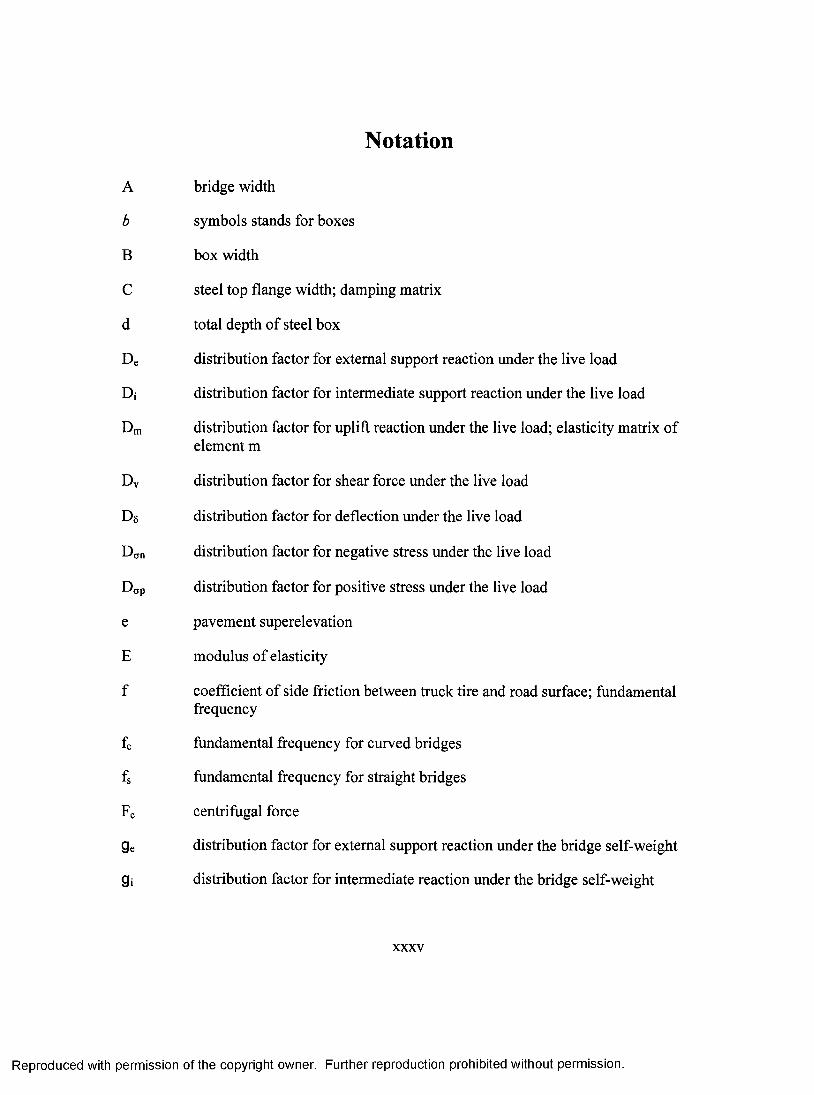
Notation
A bridge width
b symbols stands for boxes
B box width
C steel top flange width; damping matrix
d total depth of steel box
De distribution factor for external support reaction under the live load
Di distribution factor for intermediate support reaction under the live load
Dm distribution factor for uplift reaction under the live load; elasticity matrix ofelement m
Dv distribution factor for shear force under the live load
De distribution factor for deflection under the live load
D(jn distribution factor for negative stress imder the live load
Dnp distribution factor for positive stress under the live load
e pavement superelevation
E modulus of elasticity
f coefficient of side friction between truck tire and road surface; fundamentalfrequency
f c fundamental frequency for curved bridges
fs fundamental frequency for straight bridges
F c centrifugal force
Qe distribution factor for external support reaction under the bridge self-weight
9i distribution factor for intermediate reaction under the bridge self-weight
XXXV
Reproduced with permission of the copyright owner. Further reproduction prohibited without permission.
9m distribution factor for uplift reaction under the bridge self-weight
Qv distribution factor for shear force under the bridge self-weight
9 5 distribution factor for deflection under the bridge self-weight
9an distribution factor for negative stress under the bridge self-weight
9(jp distribution factor for positive stress under the bridge self-weight
H Total cross section depth including the concrete slab
I impact factor; flexural moment of inertia
Id deflection impact factor
In negative stress impact factor
Ip positive stress impact factor
Ire reaction impact factor at end-support
Iri reaction impact factor at intermediate support
Ise shear impact factor at end-support
Isi shear impact factor at intermediate support
lu uplift reaction impact factor
ki stiffness matrix for element i
K global stiffness matrix
I symbols stands for lanes
L arc length along the centreline of a bridge span
m total mass per unit length
M total mass
Nb number of boxes
Nl number of lanes
P weight of an axle
xxxvi
Reproduced with permission of the copyright owner. Further reproduction prohibited without permission.

r radius of the path on which the vehicle centre is traveling
R radius of curvature; global force vector acting in the direction of thedisplacements U
Rb forces per unit volume
Rc concentrated load at nodal C
Rd maximum dynamic response
Re maximum reaction at end-support in three-dimensional bridge obtained fromfmite-element modelling
Rea average reaction at end-support in two-span continuous idealized girder
Rj maximum reaction at intermediate support in three-dimensional bridgeobtained from fmite-element modelling
Ria average reaction at intermediate support in two-span continuous idealizedgirder
Rm minimum reaction support in three-dimensional bridge obtained from finite-clement modelling
Rs maximum static response
Rs forces per unit surface area
t sampling time
T total measuring time
ti thickness of the steel flanges and webs
tj thickness of the concrete deck slab
T„ smallest period of the finite element assemblage with n degrees of freedom
U global modal displacement vector
U virtual global modal displacement vector
V maximum shear force stress in three-dimensional bridge obtained from fmite-element modelling; vehicle speed
xxxvii
Reproduced with permission of the copyright owner. Further reproduction prohibited without permission.

Va average shear force stress in two-span continuous idealized girder
Atcr critical time step
5 maximum deflection in three-dimensional bridge obtained from fmite-elementmodelling
5a average deflection in two-span continuous idealized girder
8 virtual strain matrix for element m
s“ failure strain in the concrete model
fraction of critical damping
K = L/R span-to-radius of curvature ratio
p modification factor
On maximum negative stress in three-dimensional bridge obtained from fmite-element modelling
CTna average negative stress in two-span continuous idealized girder
Op maximum positive stress in three-dimensional bridge obtained from finite-element modelling
Opa average positive stress in two-span continuous idealized girder
o “ failure stress in the concrete model
O eigenvectors
CO circular frequency
xxxvni
Reproduced with permission of the copyright owner. Further reproduction prohibited without permission.
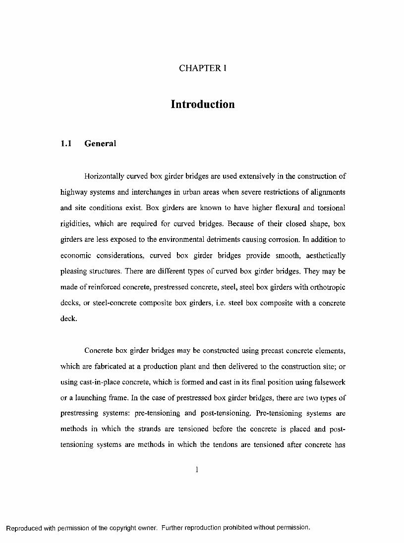
CHAPTER I
Introduction
1.1 General
Horizontally curved box girder bridges are used extensively in the construction of
highv^ay systems and interchanges in urban areas vy hen severe restrictions of alignments
and site conditions exist. Box girders are known to have higher flexural and torsional
rigidities, which are required for curved bridges. Because of their closed shape, box
girders are less exposed to the environmental detriments causing corrosion. In addition to
economic considerations, curved box girder bridges provide smooth, aesthetically
pleasing structures. There are different types of curved box girder bridges. They may be
made of reinforced eonerete, prestressed concrete, steel, steel box girders with orthotropic
decks, or steel-concrete composite box girders, i.e. steel box composite with a concrete
deck.
Concrete box girder bridges may be constructed using precast concrete elements,
which are fabricated at a production plant and then delivered to the construction site; or
using cast-in-place concrete, which is formed and cast in its final position using falsework
or a launching frame. In the case of prestressed box girder bridges, there are two types of
prestressing systems: pre-tensioning and post-tensioning. Pre-tensioning systems are
methods in which the strands are tensioned before the concrete is placed and post
tensioning systems are methods in which the tendons are tensioned after concrete has
1
Reproduced with permission of the copyright owner. Further reproduction prohibited without permission.

reached a specified strength. High tensile steel or advanced composite-fibre is usually
used as tendons in the concrete. There are also box girder bridges erected using an
orthotropic steel deck. A typical orthotropic deck bridge is formed by welding
longitudinal ribs to the transverse floor system which is supported by the main box
girders. A deck plate is then welded to the ribs.
Curved composite box girder bridges are generally used in moderate- to medium-
span bridges. Horizontal curvature of box girder may be obtained by either heat curving
or cold bending. Heat curving is typically accomplished by fabricating a straight girder in
a conventional manner and then applying thermal stresses and yielding in the top edges of
bottom flanges. Assuming the temperature is high enough, the heated edges will yield
resulting in residual stresses and straining that remains after the flanges cool. Cold
bending may be performed by using either a press or a three-roll bender. The process
must be controlled to prevent the flanges and webs from buckling or twisting out-of
plane. Bottom flanges of the box girders must be cut curved. The top flanges may be
fabricated from a single wide plate, or nested for multiple cutting from a single plate to
minimize the scrap. After preparing the webs and flanges, the webs are then welded to the
flanges and then placed in their location. Vertical camber of the girders should be
provided to allow for dead-load deflections and support rotations about an axis radial to
the girder. Cross bracing, diaphragms, and stiffeners must be provided to prevent any
distortion of the desired shape of the bridge cross section. The deck forms may be either
plywood or steel. Permanent deck forms are highly recommended inside the boxes
because of the difficulty of removing them [62]. Rebars are then placed in their position
and the concrete is cast in approved sequences to form the reinforced concrete deck,
Reproduced with permission of the copyright owner. Further reproduction prohibited without permission.
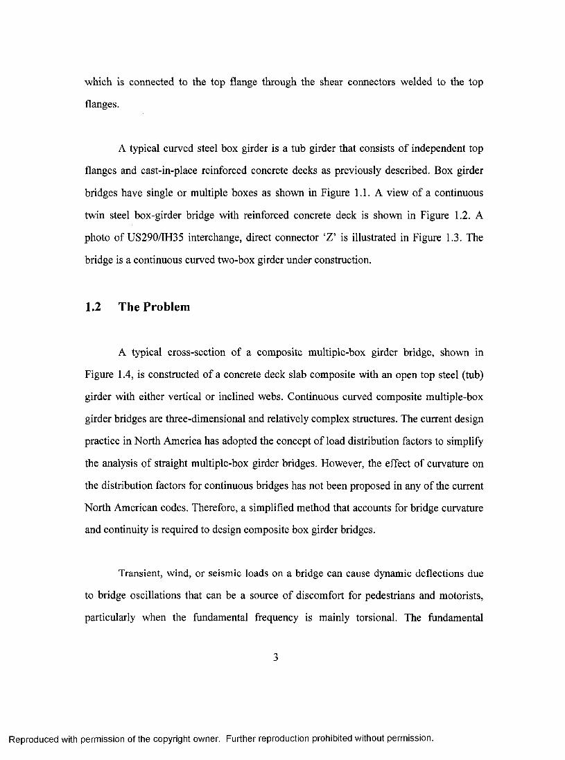
which is connected to the top flange through the shear connectors welded to the top
flanges.
A typical curved steel box girder is a tub girder that consists of independent top
flanges and cast-in-place reinforced concrete decks as previously described. Box girder
bridges have single or multiple boxes as shown in Figure 1.1. A view of a continuous
twin steel box-girder bridge with reinforced concrete deck is shovra in Figure 1.2. A
photo of US290/IH35 interchange, direct connector ‘Z’ is illustrated in Figure 1.3. The
bridge is a continuous curved two-box girder under construction.
1.2 The Problem
A typical cross-section of a composite multiple-box girder bridge, shown in
Figure 1.4, is constructed of a concrete deck slab composite with an open top steel (tub)
girder with either vertical or inclined webs. Continuous curved composite multiple-box
girder bridges are three-dimensional and relatively complex structures. The current design
practice in North America has adopted the concept of load distribution factors to simplify
the analysis of straight multiple-box girder bridges. However, the effect of curvature on
the distribution factors for continuous bridges has not been proposed in any of the current
North American codes. Therefore, a simplified method that accounts for bridge curvature
and continuity is required to design composite box girder bridges.
Transient, wind, or seismic loads on a bridge can cause dynamic deflections due
to bridge oscillations that can be a source of discomfort for pedestrians and motorists,
particularly when the fundamental frequency is mainly torsional. The fundamental
Reproduced with permission of the copyright owner. Further reproduction prohibited without permission.

frequency of a bridge is the main characteristic in investigating the effects due to dynamic
loads imposed on the structure. Experience [139] shows that high dynamic response is to
be expected only if bridge resonant frequencies coincide within the peaks of the
fundamental spectrum of the dynamic wheel load. Commercial vehicles exhibit basically
natural frequency between 2 and 5 Hz. Bridges of short to medium span length 10-100 m,
have fundamental longitudinal flexural and torsional frequencies in the range of 1 to 15
Hz. Despite the importance of obtaining the fundamental frequency for bridge structures,
there is no simplified method available in any codes in the literature to evaluate reliably
the fundamental frequency of continuous curved composite box girder bridges.
There is a tendency in most bridge codes to treat loads as static loads avoiding the
use of complicated and difficult dynamic analysis. As a result, impact factors or dynamic
amplification factors are proposed to magnify the maximum straining action exerted by a
moving vehicle to account for the dynamic effects. Impact factors recommended by the
current AASHTO Guide Specifications for Horizontally Curved Highway Bridges, 2003
[5], are based on work done a decade ago by Schelling [120] using the two-dimensional
grid technique to investigate three-dimensional bridge structures. The dynamic load
allowance suggested in the Canadian Highway Bridge Design Code, CHBDC, 2000 [20]
is basically a result of dynamic tests on several bridges other than eontinuous eurved
composite box girder bridges. Thus, the expressions for impact factors for continuous
curved composite box girder bridges based on three-dimensional bridge modeling are as
yet unavailable. Therefore, experimental and theoretical investigations on the dynamic
response o f these latter bridges are required.
Reproduced with permission of the copyright owner. Further reproduction prohibited without permission.

1.3 Objectives
Based on the problem diseussed in the previous section, the main objectives of the
conducted research work can be stated as follows:
1. Develop a three-dimensional finite element model capable of predicting
the structural response of continuous curved composite box girder
bridges;
2. Verify and substantiate the analytical model by testing in the laboratory
box-girder bridge models under different loading conditions;
3. Deduce simplified expressions for such bridges in the form of load
distribution factors for stresses, deflection, shear, and reactions;
4. Study the dynamic behaviour of these bridges when subjected to simulated
moving vehicles, and thus propose impact factors for stresses, deflection,
shear force, and reactions; and
5. Provide empirical formulas to estimate the fundamental frequency of
continuous curved composite box girder bridges.
Reproduced with permission of the copyright owner. Further reproduction prohibited without permission.

1.4 Scope
To achieve the aforementioned objectives, the scope of this research work
includes the following:
1. Literature review of the analytieal methods, previous experimental and
theoretical research work, and codes of practice for straight and curved
box girder bridges;
2. Develop three-dimensional finite element bridge models using the
commercially available finite element eomputer program “ABAQUS”;
3. Test straight and curved bridge models made of twin-box girders
continuous over two-equal-span, having a cast-in concrete deck;
4. Compare the finite element model predictions with the experimental
findings of the laboratory tested bridge models for various load cases to
verify the finite element model and provide information about the
nonlinear response of box girder bridges;
5. Undertake several parametric studies on the main variables that may affect
the load distribution factors, impact factors, and fundamental frequeneies
of such bridges;
Reproduced with permission of the copyright owner. Further reproduction prohibited without permission.

6. Deduce empirical formulas for load distribution and impact factors for
stresses, deflection, shear, and reaction, and fundamental frequencies of
continuous curved concrete deck on multiple steel box girder bridges.
1.5 Outline of the Dissertation
In this dissertation a literature review of the earlier analytical and experimental
work on box girder bridges is presented in Chapter II. The finite element analysis is
described in Chapter III. In that chapter, linear static, free-vibration, and dynamic
analyses, and idealizing and modeling of the bridge components are also incorporated and
explained. Chapter IV includes the details of the experimental work conducted on two
bridge models, including instrumentations, loading systems, and the test procedure. In
Chapter V, the comparison between the experimental results and those predicated by the
finite element modeling is undertaken. Also, the nonlinear structural response is
examined analytically and experimentally. Chapter VI explains the parametric studies
conducted on the prototype bridges. Chapter VII presents the results of the load
distribution factors and the effects of various parameters on these factors. Chapters VIII
and IX deal with the results obtained for the impact factors and fundamental frequency,
respectively. The summary, conclusions and recommendations for further research are
presented in Chapter X.
Reproduced with permission of the copyright owner. Further reproduction prohibited without permission.
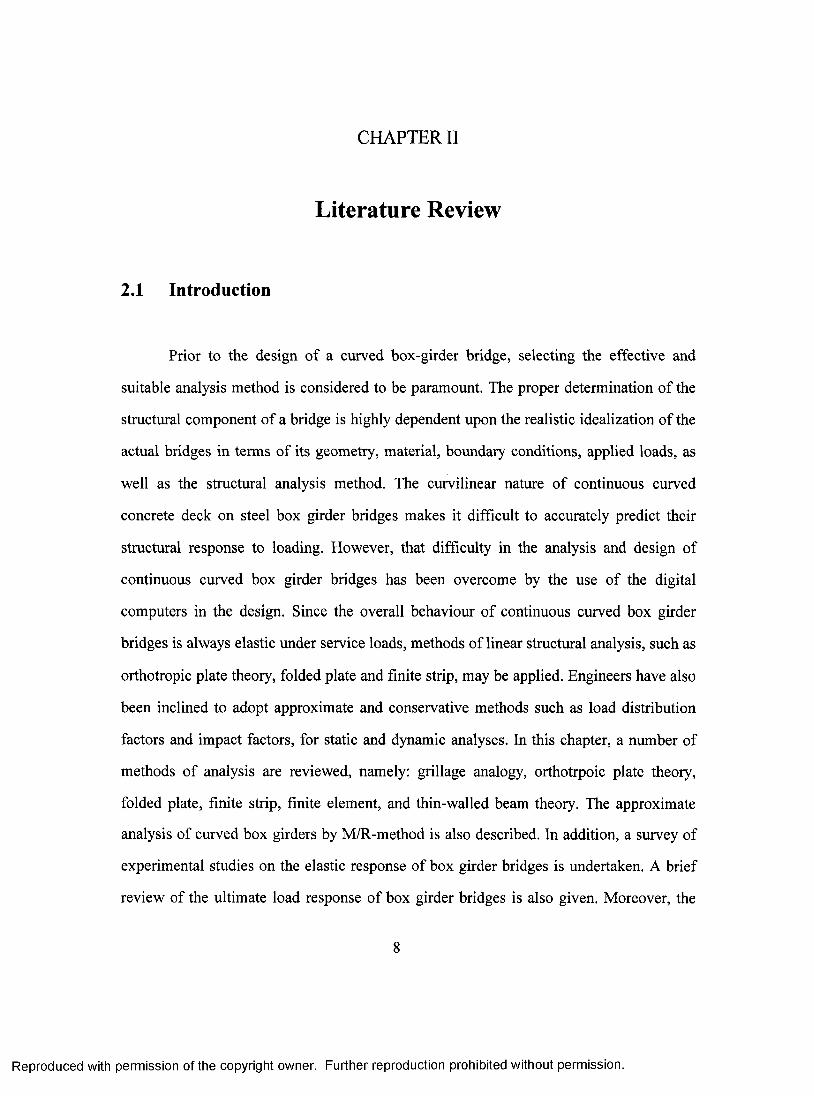
CHAPTER II
Literature Review
2.1 Introduction
Prior to the design of a curved box-girder bridge, selecting the effective and
suitable analysis method is considered to be paramount. The proper determination of the
structural component of a bridge is highly dependent upon the realistic idealization of the
actual bridges in terms of its geometry, material, boundary conditions, applied loads, as
well as the structural analysis method. The curvilinear nature of continuous curved
concrete deck on steel box girder bridges makes it difficult to accurately predict their
structural response to loading. However, that difficulty in the analysis and design of
continuous curved box girder bridges has been overcome by the use of the digital
computers in the design. Since the overall behaviour of continuous curved box girder
bridges is always elastic under service loads, methods of linear structural analysis, such as
orthotropic plate theory, folded plate and finite strip, may be applied. Engineers have also
been inclined to adopt approximate and conservative methods such as load distribution
factors and impact factors, for static and dynamic analyses. In this chapter, a number of
methods of analysis are reviewed, namely: grillage analogy, orthotrpoic plate theory,
folded plate, finite strip, finite element, and thin-walled beam theory. The approximate
analysis of curved box girders by M/R-method is also described. In addition, a survey of
experimental studies on the elastic response of box girder bridges is undertaken. A brief
review of the ultimate load response of box girder bridges is also given. Moreover, the
8
Reproduced with permission of the copyright owner. Further reproduction prohibited without permission.

results of a earlier work concerning load distribution, impact factors and fundamental
frequencies of box girder bridges are presented.
2.2 Analytical Methods for Box Girder Bridges
Several methods are available for the analysis of box girder bridges. In each
analysis method, the three-dimensional bridge structure is usually simplified by means of
assumptions in the geometry, materials and the relationship between its components. The
accuracy of the structural analysis is dependent upon the choice of a particular method
and its assumptions. A review of different analytical methods for concrete box girder
bridges has been published by Scordelis [121] with reference to a large number of
computer programs developed at the University of California, Berkeley. Kirstek [88] has
discussed the theoretical aspect of some of the methods. Also, a comparative study of the
various methods available for the analysis of straight prismatic single-cell box girders has
been presented by Maisel and Roll [93]. A brief review of the aforementioned methods is
presented in the following sections.
2.2.1 Grillage Analogy Method
Grillage analysis has been applied to multiple cell boxes with vertical and sloping
webs and voided slabs. In this method, the bridge deck is idealized as a grid assembly.
The continuous curved bridge is modelled as a system of discrete curved longitudinal
members intersecting orthogonally with transverse grillage members. As a result of the
fall-off in stress at points remote from webs due to shear lag, the slab width is replaced by
a reduced effective width over which the stress is assumed to be uniform. The equivalent
Reproduced with permission of the copyright owner. Further reproduction prohibited without permission.

stiffnesses of the continuum are lumped orthogonally along the grillage members. One
problem which arises by using the grillage analogy method is in determining the effective
width of the slab to include the shear lag effects. Another difficulty of this method lies in
estimating the torsional stiffness of the closed cells. Approximate technique may be used
to model the torsional stiffness of closed cells by an equivalent I-beam torsional stiffness.
This technique, established by Evans and Shanmugam [50], provides satisfactory results.
2.2.2 Orthotropic Plate Theory Method
In the orthotropic plate theory method, the interaction between the concrete deck
and the curved girder of a box girder bridge is considered. The stiffness of the diaphragms
is distributed over the girder length. The stiffnesses of the flanges and girders are lumped
into an orthortropie plate of equivalent stiffness. However, the estimation of the flexural
and torsional stiffnesses is considered to be one major problem in this method. Also, the
evaluation of the stresses in the slab and girder presents another difficulty in adopting this
approach. In spite of that Cheung [33] has suggested this method for multiple-girder
eurved bridges with high torsional rigidity. The Canadian Highway Bridge Design Code
[20] has recommended using this method mainly for the analysis of straight box girder
bridges.
2.2.3 Folded Plate Method
A multiple-box girder bridge can be modeled as a folded system which consists of
longitudinal plate elements interconnected at joints along their longitudinal edges and
simply-supported at both ends by diaphragms which are infinitely stiff in their planes and
10
Reproduced with permission of the copyright owner. Further reproduction prohibited without permission.
perfectly flexible perpendicular to these planes. Any arbitrary longitudinal joint loading
can be resolved into harmonic component of the loading using Fourier series. Then, a
direct stiffness analysis can be performed for each component. Originally, the folded plate
method is limited to simply supported box girder and no intermediate diaphragms are
assumed. This method produces solutions for linear elastic analysis of a box girder
bridge, within the scope of the assumptions of the elasticity theory. The method has been
used to analyze cellular structures by Al-Rifaie and Evans [2], Evans [49], and Meyer and
Scordelis [95]. Canadian Highway Bridge Design Code [20] restricted the use of this
method to bridges with support conditions closely equivalent to a line support. One of the
major shortcomings of the folded plate method is the large computational effort required
and its complexity.
2.2.4 Finite Strip Method
The finite strip method discretizes the bridge into a longitudinal number of strips,
running from one end support to the other. The strips are connected along their
longitudinal edges by nodal lines. The stiffness matrix is then calculated for each strip
based upon a displacement function in terms of Fourier series, rather than on the theory of
elasticity. Similar to the folded plate method, in the finite strip method the direct stiffness
harmonic analysis is performed. The finite element method is basically different from the
strip method in terms of the assumed displacement interpolation functions. Unlike the
finite element method, the displacement functions for the corresponding finite strip are
assumed as combination o f harmonics varying longitudinally and polynomialy in the
transverse direction. Therefore, the strip method is considered as a transition between the
folded plate method and the finite element method. The method is well suited and is a
11
Reproduced with permission of the copyright owner. Further reproduction prohibited without permission.

powerful technique for the analysis of orthotropic and circularly curved plate elements for
which direct application of the theory of elasticity becomes too involved. In 1968,
Cheung [32] introduced this method and then in 1971 Cheung and Cheung [28] applied
the finite strip method for curved box girder bridges. In 1974, Kabir and Scordelis [79]
developed a finite strip computer program to analyze curved continuous span cellular
bridges, with interior radial diaphragms, on supporting planar frame bents. Free vibration
of curved and straight beam-slab and box-girder bridges was conducted by Cheung and
Cheung [34] using the finite strip method. In 1978, the method was adopted by Cheung
and Chan [27] to determine the effective width of the compression flange of straight
multi-spine and multi-cell box girder bridges. Cheung [26] in 1984 used a numerical
technique based on the finite strip method and the force method for the analysis of
continuous curved box girder bridges. In 1989, Ho et al. [71] used the finite strip to
analyze three different types of simply supported highway bridges, slab-on-girder, two
cell box girder, and rectangular voided slab bridges.
The basic advantage of the finite strip method is that it requires small computer
storage and relatively little computation time. Although the finite strip method has
broader applicability as compared to folded plate method, the method is still limited to
simply supported prismatic structures. For multi-span bridges, Canadian Highway Bridge
Design Code [20] restricts the method to those with interior supports closely equivalent to
line supports and isolated columns supports.
12
Reproduced with permission of the copyright owner. Further reproduction prohibited without permission.

2.2.5 Finite Element Method
The finite element technique is being extensively applied to complicated
structures and is generally the most powerful and versatile as well as accurate numerical
tool of all the available methods. The finite element method has rapidly become a very
popular technique for the computer solution of a box girder bridge of arbitrary plan
geometry and variable cross section. In the finite element analysis the structure is
modelled using suitable finite elements by subdividing its solution domain into discrete
elements. A large number of elements have been developed for use in the finite element
technique. These finite elements may be one-dimensional beam-type elements, two-
dimensional plate or shell elements or even three-dimensional solid elements.
Since the structure is composed of several finite elements interconnected at nodal
points, the individual element stiffness matrix, which approximates the behaviour in the
continuum, is assembled based on assumed displacement or stress patterns. Then, the
nodal displacements and hence the internal stresses in the finite element are obtained by
the overall equilibrium equations. By using adequate mesh refinement, results obtained
from finite element model usually satisfy compatibility and equilibrium [152].
Aneja and Roll [8, 117] have used the finite element technique for horizontally
curved bridge with a box cross-section using flat plate element with curved boundaries
for discretizing the flanges and flat rectangular elements for the webs. The analytical
results showed poor agreement with the experimental findings, because the elements used
did not have sufficient degrees of freedom at their nodes to account for rotation around all
axes; further the web modelling with flat rectangular element did not seem to be
13
Reproduced with permission of the copyright owner. Further reproduction prohibited without permission.

sufficiently accurate. Chu and Pinjarkar [36] in 1971 developed finite element
formulation for curved box girder bridges consisting of horizontal sector plates and
vertical cylindrical shell elements. In 1972, Wiliam and Scordelis [144] analyzed cellular
structures of constant depth with arbitrary plan geometry using quadrilateral element in
the finite element analysis. Bazant and El Nimeiri [11] in 1974 attributed the problems
associated with the neglect of curvilinear bovmdaries in the elements used to model
curved box beams by the loss of continuity at the end cross-section of two adjacent
elements meeting at an angle. Instead of developing curvilinear element boundaries, they
developed the skew-ended finite element with shear deformation using straight elements.
Fam and Turkstra [53, 54] and Fam [52] adopted the finite element method for static and
free vibration analysis of box girders with orthogonal boundaries and arbitrary
combination of straight and horizontally curved sections, the analysis has been shown to
be reliable and efficient. Four-node plate bending annular elements were chosen to
idealize the flange members and conical elements for the inclined web members. In 1995,
Galuta and Cheung [60] combined the boundary element with the conventional finite
element method to analyze box girder bridges. The bending moments and vertical
deflection were found to be in good agreement when compared with the finite strip
solution. Davidson et al. [40] in 1996 utilized the finite element method to develop a
detailed model for horizontally curved steel I-girder bridges. In 1998, Sennah and
Kermedy [128] conducted an extensive parametric study on composite multi-cell box
girder bridges using the finite element analysis. The results obtained from the finite
element method were in good agreement with the experimental findings.
The numerical effectiveness, accuracy as well as the flexibility of the method in
linear, non-linear, static or dynamic analyses has been well established. Therefore, many
14
Reproduced with permission of the copyright owner. Further reproduction prohibited without permission.

investigators have been attracted to adopt the finite element method to analyze the
complex mechanics of arbitrary box girder bridges. Canadian Highway Bridge Design
Code has recommended the finite element method for all type of bridges.
2.2.6 Thin-Walled Beam Theory Method
Thin-walled beam theory applicable to box beam has been established by Vlasov
[141] and elaborated by Dabrowski [39] and others. The theory assumes non-distortional
cross-section and, hence, does not account for all warping or bending stress. The
predication of shear lag or the response of deck slabs to local wheel load cannot be
obtained using the theory. In 1966, Kolbrunner and Hajden [84] treated thin-walled beam
structures similar to Vlasov but in more general form by including shear deformation for
closed thin-walled cross sections. The load-deformation response of curved box girder,
which considers bending, torsion and warping deformations, as developed by Vlasov, was
used to predict the behaviour of the cross section assumed to retain their shape xmder
loads [106, 67, 69, 100]. In 1985, Maisel [92] extended Vlasov’s thin-walled beam theory
to account for torsional, distortional, and shear lag effects of straight, thin-walled cellular
box beams. Mavaddat and Mirza [94] implemented formulations into computer programs
to analyze straight concrete box beams with one, two, or three cells and side cantilevers
over a simple span or two spans with symmetric mid-span loading. Li [90] and Razaqpur
and Li [113, 114, 115] developed a box girder finite element, which includes extension,
torsion, distortion, and shear lag analysis of straight, skew, and curved multi-cell box
girders using thin-walled finite element based on Vlasov’s theory. Exact shape functions
were used to eliminate the need for dividing the box into many elements in the
longitudinal direction. The results of the proposed element agreed well with those results
15
Reproduced with permission of the copyright owner. Further reproduction prohibited without permission.

obtained from full three-dimensional shell finite element analysis. For both static and
dynamic analyses of multi-cell box girder bridges, Vlasov’s thin-walled beam theory was
cast in a finite element formulation and exact shape function was used by El-Azab [48] to
derive the stiffness matrix.
2.2.7 M/R-Method
The M/R-method provides a means to account for the effect of curvature in curved
box girder bridges. The basic concept behind this method is to load a conjugate beam
with a distributed loading. The load on the conjugated beam is equal to the moment in the
real simple or continuous beam induced by the applied load divided by the radius of
curvature of the girder. The reactions of supports are obtained and thus the shear diagram
can be drawn representing the internal torque diagram of the curved beam. The method
and suggested limitations on its use were discussed by Tung and Fountain [140].
However, the method may be restrictive because the box girder is idealized as a 2-D
beam. The vertical reactions at the interior supports on the concave side of a continuous
span bridge may be significantly underestimated by the M/R-method.
2.3 Experimental Elastic Studies
In order to verify the analytical solutions and computer programs developed,
several experimental studies were conducted on box girder bridges. Occasionally,
experimental studies were reported on field-testing of existing box girders. However, the
majority of experimental tests have taken place in the laboratories on small scale bridge
models.
16
Reproduced with permission of the copyright owner. Further reproduction prohibited without permission.
In 1975, Kissane and Beal [83] performed a field test program initiated by the
Engineering Research and Development Bureau of the New York State Department of
Transportation. The program was to evaluate the behaviour of a two-span, continuous,
curved box-girder bridge under dead and static live loads. Yoo et al. [148] in 1976
measured the response of a three-span continuous curved box girder bridge designed for
two-lane traffic. The bridge was tested when the concrete deck was cast and later, when
the construction of the bridge was completed. In 1979, Brennan and Mandel [16]
conducted an experimental study on eight different small-scale horizontally curved
bridges. Six models were 1-section girder bridges and two were three-span two box-girder
bridges. The experimental findings were used to verify a computer program developed at
Syracuse University. In 1982, Buckle and Hood [19] performed an experimental test on a
continuous curved box girder model to validate the finite element method results. In
1987, Xi-jin and De-rong [145] tested a three-span conditions curved box girder bridge.
The main objective of the model was to detect the characteristics of the curved box-girder
under various loading continuous and to further verify the accuracy of the finite strip
method as well as a computer program used in the analytical analysis. In 1988, Siddiqui
and Ng [134] examined two straight plexiglass, single cell, box girder bridge models to
investigate the influence of the transverse diaphragms on the behaviour of the box
section. Ng et al. [101] in 1992 conducted on experimental study of a 1/24 scale
composite concrete deck aluminium four-cell model of the Cyrville Road Bridge overpass
east of Ottawa, under various OHDBC truck loading conditions. The prototype was a
two-span continuous two-lane concrete curved four-cell box girder bridge. Green [61] in
1978, Branco [14] in 1985, and Branco and Green [15] in 1985 conducted experimental
study to examine the effect of construction loadings, as well as the bracing configurations
of simple-span open and quasi-closed cross-section beams. The results from the tests
17
Reproduced with permission of the copyright owner. Further reproduction prohibited without permission.
were used to verify those obtained from the analytical study. In 1985, McGill University
[43] conducted an experimental study of a 1/10.45 scale two-span continuous straight
composite concrete deck-steel box girder bridge. In 1997, Ebeido and Kennedy [47]
conducted an experimental study on three continuous skew composite steel concrete
bridge models with two unequal spans. In 1998, Setmab [124] tested five straight and
curved deck-steel three-cell bridge models vmder various static loading conditions and
free vibration tests. Four models were simply-supported and the fifth was a two-equal-
span continuous bridge model. The results obtained from the experimental work were
utilized to verify the finite element model.
2.4 Experimental Up-to-Collapse Studies
Fewer experimental studies have dealt with the up-to-collapse response of straight
and curved box girder bridges. Dogaki et al. [45] in 1979 investigated experimentally the
ultimate behaviour of two horizontally curved steel single-cell box girder bridge models
under two concentrated loads. In 1979, Heins and Humphnay [64] tested up-to-failure a
series of box beam models, composed of top steel flanges, steel webs, steel bottom
flanges and cross-bracings. Some of the beam models had concrete deck, while the rest
did not. An interaction, non-dimensional, equation was developed based on the
experimental findings to predict the load distribution factor of curved steel box girders.
Scordelis et al. [122] tested a two-span, four-cell, reinforced concrete box girder bridge
up-to-collapse. Results obtained from that test agreed well with a three-dimensional
grillage model and a computer program to estimate the non-linear response of multi-cell
reinforced concrete box girder bridges subjected to static loading. In 1985, McGill
University [43] tested a composite deck-steel box girder bridge up to failure. Owens et al.
18
Reproduced with permission of the copyright owner. Further reproduction prohibited without permission.

[110] conducted similar experimental study on curved composite concrete-deck steel
multi-spine box girders assembly. In 1994, Soliman [135] performed experimental studies
on straight and curved reinforced concrete single-cell box girder bridge models to
investigate the influence of diaphragms on the bridge behaviour. In 1997, Ebeido and
Kennedy [47] tested three continuous skew composite bridges up to collapse using
simulated truck loads applied on two lanes. Theoretical studies were also undertaken to
better understand the non-linear behaviour as well as the local buckling of individual steel
plates of straight and curved box girder bridges. In 1995, Yabuki et al. [146] developed a
numerical method to estimate the effect of the local buckling in plates and distortional
phenomenon on the non-linear response and ultimate strength of thin-walled curved steel
box girders. In 1998, Sennah [124] employed the finite element method to predict the
non-linear response of composite concrete-deck steel cellular bridges.
2.5 Load Distribution Factors
The distribution of dead load and wheel load on highway bridges is the most
important method in selecting the member size. Engineers can predict the bridge response
by applying the load distribution factor concept. Prior to 1959, design of concrete box-
girder bridges was based on the distribution factor approach in which individual 1-section
were assumed loaded with S/5 wheel lines of a standard H-series vehicle [3], where S is
the spacing (in feet) between centrelines of webs [41]. In 1959, California Design
Engineers [123] suggested to American Association of State Highway Officials
(AASHO) to change this distribution factor to S/7. A computer program was written by
Johnston and Mattock [78] in 1967 to study the lateral distribution of load in simple span
composite box girder bridges without transverse diaphragms or internal stiffeners. In
19
Reproduced with permission of the copyright owner. Further reproduction prohibited without permission.

1968, Fountain and Mattock [56] implemented the folded plate method in a computer
program to calculate the lateral distribution of loads in 24 simply supported composite
multiple box girder bridges. The results of the folded plate computer program were
verified by testing one-quarter model of a two-lane, 24.4 m span bridge with three box
girders and one-fifth model of a two-lane, 30.4 m span bridge with two box girders, under
AASHTO truck loadings. The results obtained from the computer program were used to
develop an expression for the live load bending moment distribution factor for each
girder as a function of the roadway width and the number of box girders. The results from
the research program by Fountain and Mattock formed the basis for the lateral
distribution factors for bending moment currently adopted by AASHTO [3] and Ontario
Highway Bridge Design Code in 1983 [108] for multiple box girder bridges. The
application of the deduced expression, however, was limited to bridges having the ratio of
the number of lanes to number of boxes within 0.5-1.5. The results were obtained based
on ratio of relatively limited investigation of a number of bridges considering only the
number of lanes and number of boxes as variables. Most importantly, the curvature and
the continuity effects were not considered in the study. In 1969, Scordelis and Meyer
[123] published an extensive study of wheel load distribution in concrete box girder
bridges and developed formulas that included parameters thought to influence the load
distributions; i.e., span length, number of lanes, cell width, and number of cells.
In 1978, Heins [63] collected the detailed geometry of 82 bridges built until 1975.
Typical composite sections were constructed from these available data. A computer
program developed by Heins and Olenick [67] was utilized to obtain the response o f nine
braced and nine composite sections of horizontally curved multiple box girder bridges. In
1984, Heins and Jin [65] carried out a design-oriented research study on live load
20
Reproduced with permission of the copyright owner. Further reproduction prohibited without permission.

distribution of curved composite I-girder bridges. A modification factor to the straight
girder moment distribution developed by Fountain and Mattock [56] was proposed as a
function of the radius of curvature. Bridges with span lengths of 15, 30 and 45 m only
were included. In 1980, Mukherjee and Trikha [99] developed a set of design coefficients
for twin cell curved box girder reinforced concrete bridges using the finite strip method.
These coefficients were for moment, shear, transverse moment, and vertical deflection
under the webs. However, these coefficients were limited only for bridges of two-lanes
with span length between 20 and 40 m, and radius of curvature between 45 and 150 m. In
1988, Nutt et al. [104] developed a set of equations for moment distribution in straight,
reinforced and prestressed concrete, multi-cell box girder bridges as a function of number
of lanes, number of cells, cell width, and span length. In 1989, Ho et al. [71] investigated
straight simply-supported, two-cell box girder and rectangular voided slab bridges using
the finite strip method. As a result of that research, formulas were deduced for the ratio of
the maximum longitudinal bending moment to the equivalent beam moment. However,
the application of the formulas was limited to straight two-cell bridge sections made of
either steel or concrete with span lengths of bridges up to 40 m in case of two-lane, 50 m
in the case of three-lane, and 67 m in the case of four-lane. In 1986, Brockenbrough [18]
derived load distribution factors using the finite element method for curved composite 1-
girder bridges as a function of the span length, radius of curvature, girder spacing, and
cross-bracing spacing. In 1985 and 1992, Bakht and Jaeger [9, 10] presented a particular
case of multi-spine bridges having at least three spines having zero transverse bending
stiffness, with the load transfer between the various spines through transverse shear. They
proposed simplified expressions for the load distribution factors for bending moment and
shear. These expressions formed the basis for the live load distribution factors used by the
OHBDC [109] for multi-spine bridges.
21
Reproduced with permission of the copyright owner. Further reproduction prohibited without permission.

In 1992, Zokaie et at. [151] developed moment and shear distribution factors for
moment and shear for reinforced and prestressed concrete box girder bridges. The
proposed expressions were adopted by the current AASHTO LRFD [7] for straight
concrete bridges. In 1994, Noramandin and Massicotte [102] used the finite element
method in determining the distribution patterns for bending moment and shear force in
simply supported straight multi-spine box girder bridges. The effects of internal
diaphragms, external bracings, inclined webs and vehicle loading were studied for such
bridges. They concluded that the internal diaphragms contributed largely to the reduction
of the cross section distortion. However, the external bracing did not significantly
influence the distribution characteristics for bending moments and shear force. In 1995,
Cheung and Foo [29] studied the behaviour of simply supported curved and straight box
girder bridges subjected to OHBDC truck loading. The finite strip element was used in
the parametric study to develop expression for the moment distribution factors of such
bridges as function of span length, number of lanes, box spacing, and radius of curvature.
The effects of the number of boxes and dead load distribution were not included in the
study. Dean [42] in 1994 and Fu and Yang [57] in 1996 investigated the torsional
distribution on multi cellular members. In 1996, Brighton et al. [17] studied the live load
distribution for a new type of concrete double cell box girders proposed for a
prefabricated bridge system for the rapid construction of short-span bridges.
In 1997, Foinquinos et al. [55] studied the influence of intermediate diaphragms
on the live load distribution of straight multiple steel box girder bridges. The results
showed that using only two cross frames sufficed to redistribute the live load stresses and
adding more cross frames did not improve the distribution of live load. In 1998, Mabsout
et al. [91] presented finite element results of a study of the effect of continuity on the
22
Reproduced with permission of the copyright owner. Further reproduction prohibited without permission.
wheel load distribution factors for I-girder bridges. Sennab [124] in 1998 and Sennab and
Kennedy [126, 128] in 1999 eonducted an extensive parametric study on curved simply
supported composite concrete deck-steel cellular bridges using the finite element analysis.
Empirical expressions for moment, shear and axial forces in the bracing system were
developed. Nour [103] in 2000 and Sennab et al. [131] in 2003 adopted the finite element
method to deduce empirical formulas for load distribution factors in curved composite
deck-steel multiple-spine box girder bridges. However, the proposed equations were
limited to simply supported box girder bridges. Sennab and Kermedy [129, 130]
presented a comprehensive literature review in analyzing of box-girder bridges.
The superseded version of the Ontario Highway Bridge Design Code [109] and
Canadian Standard for Design of Highway Bridges [21], OHBDC, draft [107], and
CHBDC [20] allow the treatment of a curved bridge as a straight one if the ratio (L^/bR)
is not greater than 1.0, where L is the span length, R is the mean radius of curvature and b
is half-width of the bridge. However, there are no expressions for the more common cases
where the above ratio is greater than 1.0. The superseded 1993 version of the AASHTO
Guide Specifications for Horizontally Curved Highway Bridges [4] ignored the curvature
effect in determining primary bending moments when the subtended angle did not exceed
5°. However, AASHTO 2003 [5] did not propose any other expression for load
distribution factors. Therefore, research work to investigate the live load distribution in
continuous curved concrete deck on multiple steel box girder bridges is required to
provide engineers with simplified method to design such bridges. This is the first
objective for the parametric study.
23
Reproduced with permission of the copyright owner. Further reproduction prohibited without permission.
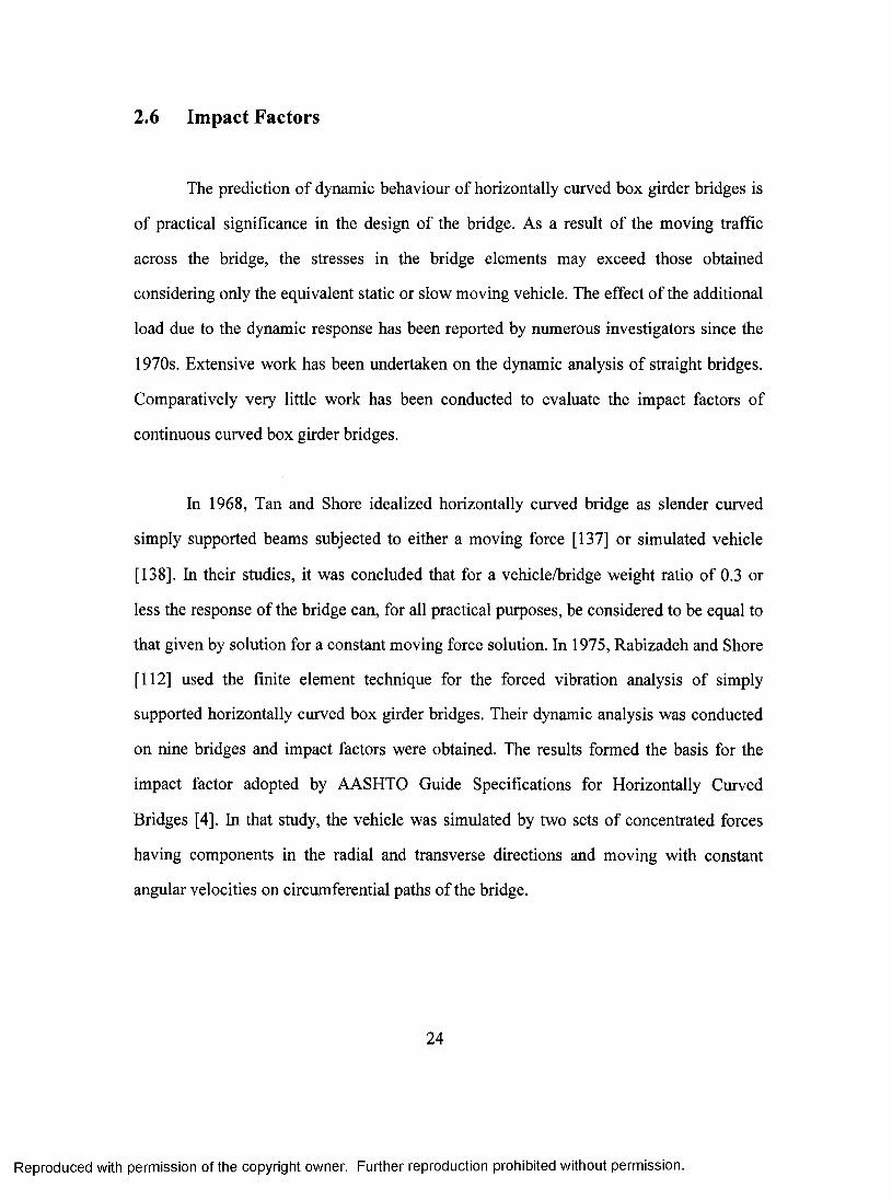
2.6 Impact Factors
The prediction of dynamic behaviour of horizontally curved box girder bridges is
of practical significance in the design of the bridge. As a result of the moving traffic
across the bridge, the stresses in the bridge elements may exceed those obtained
considering only the equivalent static or slow moving vehicle. The effect of the additional
load due to the dynamic response has been reported by numerous investigators since the
1970s. Extensive work has been undertaken on the dynamic analysis of straight bridges.
Comparatively very little work has been conducted to evaluate the impact factors of
continuous curved box girder bridges.
In 1968, Tan and Shore idealized horizontally curved bridge as slender curved
simply supported beams subjected to either a moving force [137] or simulated vehicle
[138]. In their studies, it was concluded that for a vehicle/bridge weight ratio of 0.3 or
less the response of the bridge can, for all practical purposes, be considered to be equal to
that given by solution for a constant moving force solution. In 1975, Rabizadeh and Shore
[1 1 2 ] used the finite element technique for the forced vibration analysis of simply
supported horizontally curved box girder bridges. Their dynamic analysis was conducted
on nine bridges and impact factors were obtained. The results formed the basis for the
impact factor adopted by AASHTO Guide Specifications for Horizontally Curved
Bridges [4]. In that study, the vehicle was simulated by two sets of concentrated forces
having components in the radial and transverse directions and moving with constant
angular velocities on circumferential paths of the bridge.
24
Reproduced with permission of the copyright owner. Further reproduction prohibited without permission.
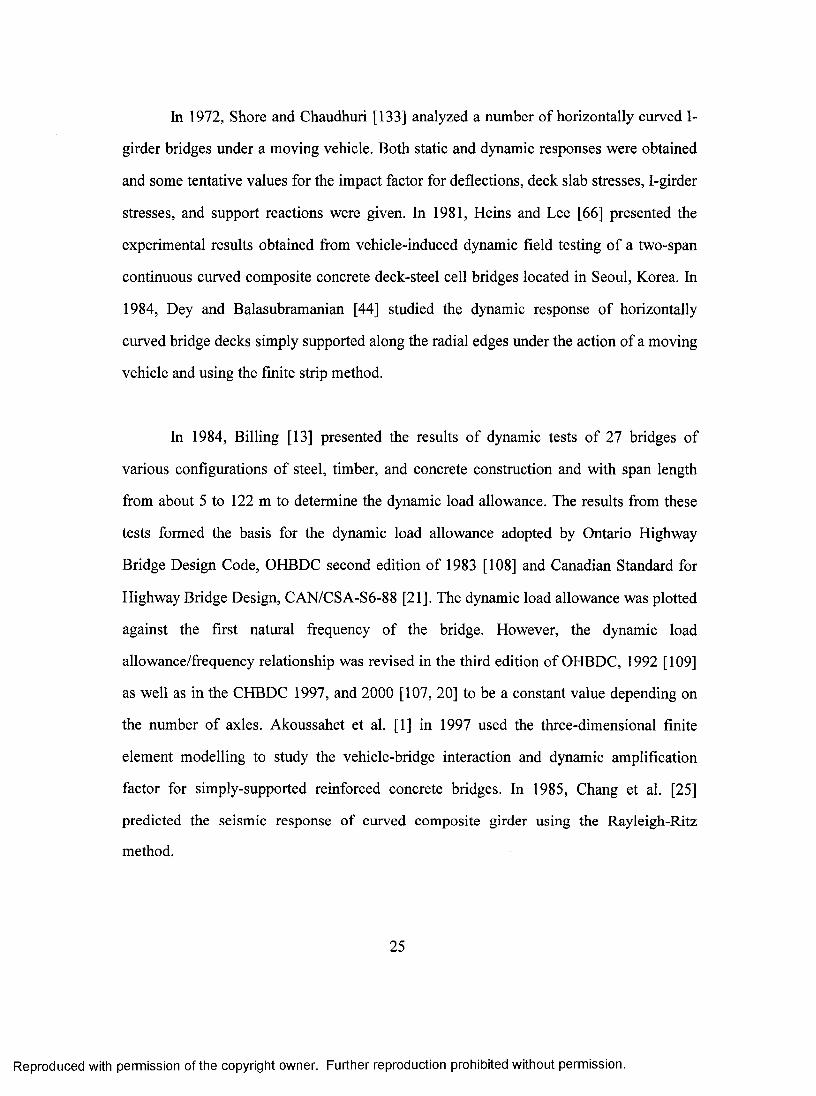
In 1972, Shore and Chaudhuri [133] analyzed a number of horizontally curved 1-
girder bridges under a moving vehicle. Both static and dynamic responses were obtained
and some tentative values for the impact factor for deflections, deck slab stresses, 1-girder
stresses, and support reactions were given. In 1981, Heins and Lee [6 6 ] presented the
experimental results obtained from vehicle-induced dynamie field testing of a two-span
continuous curved composite concrete deck-steel cell bridges located in Seoul, Korea. In
1984, Dey and Balasubramanian [44] studied the dynamic response of horizontally
curved bridge deeks simply supported along the radial edges under the action of a moving
vehicle and using the finite strip method.
In 1984, Billing [13] presented the results of dynamic tests of 27 bridges of
various configurations of steel, timber, and concrete construction and with span length
from about 5 to 122 m to determine the dynamic load allowance. The results from these
tests formed the basis for the dynamic load allowance adopted by Ontario Highway
Bridge Design Code, OHBDC second edition of 1983 [108] and Canadian Standard for
Highway Bridge Design, CAN/CSA-S6 - 8 8 [21]. The dynamic load allowance was plotted
against the first natural frequency of the bridge. However, the dynamic load
allowance/frequency relationship was revised in the third edition of OHBDC, 1992 [109]
as well as in the CHBDC 1997, and 2000 [107, 20] to be a constant value depending on
the number of axles. Akoussahet et al. [1] in 1997 used the three-dimensional finite
element modelling to study the vehicle-bridge interaction and dynamic amplification
factor for simply-supported reinforced concrete bridges. In 1985, Chang et al. [25]
predicted the seismic response of curved composite girder using the Rayleigh-Ritz
method.
25
Reproduced with permission of the copyright owner. Further reproduction prohibited without permission.
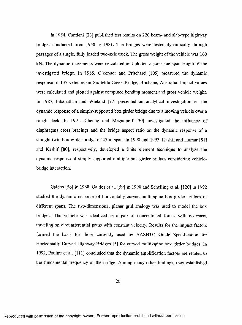
In 1984, Cantieni [23] published test results on 226 beam- and slab-type highway
bridges conducted from 1958 to 1981. The bridges were tested dynamically through
passages of a single, fully loaded two-axle truck. The gross weight of the vehicle was 160
kN. The dynamic increments were calculated and plotted against the span length of the
investigated bridge. In 1985, O’connor and Pritchard [105] measured the dynamic
response of 137 vehicles on Six Mile Creek Bridge, Brisbane, Australia. Impact values
were calculated and plotted against computed bending moment and gross vehicle weight.
In 1987, Inbanathan and Wieland [77] presented an analytical investigation on the
dynamic response of a simply-supported box girder bridge due to a moving vehicle over a
rough deck. In 1991, Cheung and Megnounif [30] investigated the influence of
diaphragms cross bracings and the bridge aspect ratio on the dynamie response of a
straight twin-box girder bridge of 45 m span. In 1990 and 1992, Kashif and Humar [81]
and Kashif [80], respectively, developed a finite element technique to analyze the
dynamic response of simply-supported multiple box girder bridges considering vehicle-
bridge interaction.
Galdos [58] in 1988, Galdos et al. [59] in 1990 and Schelling et al. [120] in 1992
studied the dynamic response of horizontally curved multi-spine box girder bridges of
different spans. The two-dimensional planar grid analogy was used to model the box
bridges. The vehicle was idealized as a pair of concentrated forces with no mass,
traveling on circumferential paths with constant velocity. Results for the impact factors
formed the basis for those currently used by AASHTO Guide Specification for
Horizontally Curved Highway Bridges [5] for curved multi-spine box girder bridges. In
1992, Paultre et al. [ I l l ] concluded that the dynamic aipplification factors are related to
the fundamental frequency of the bridge. Among many other findings, they established
26
Reproduced with permission of the copyright owner. Further reproduction prohibited without permission.
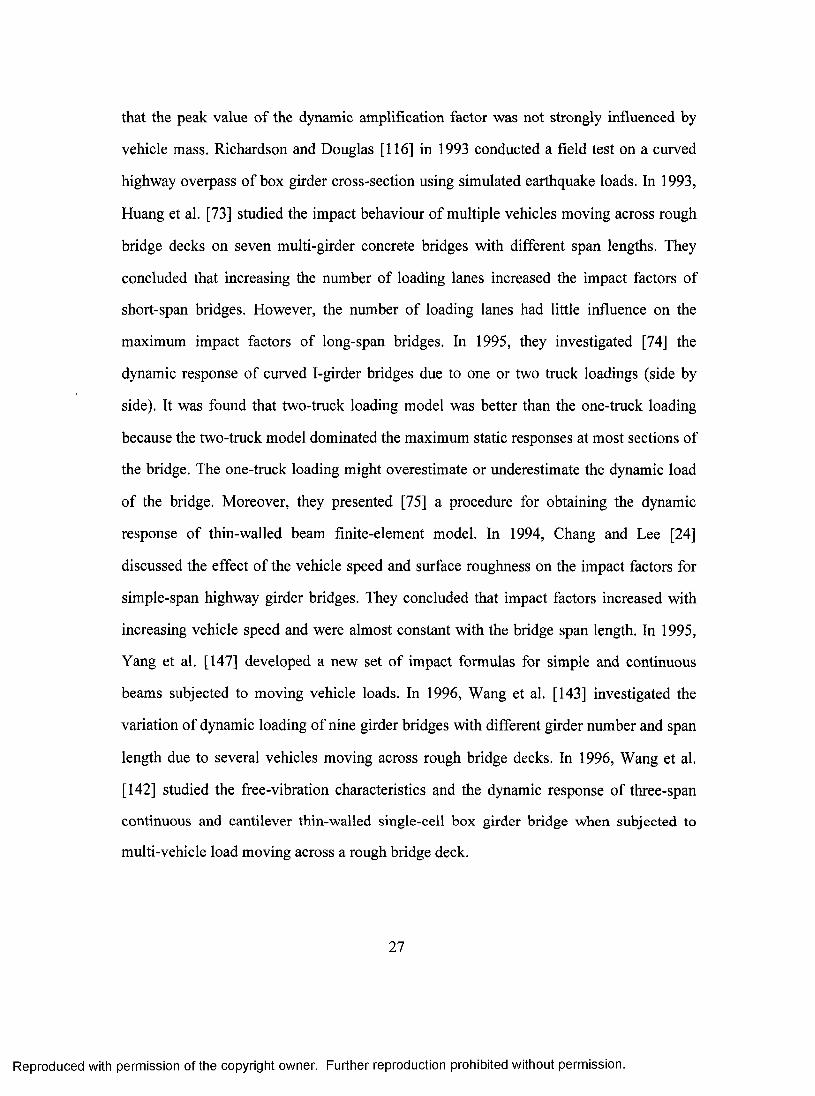
that the peak value of the dynamic amplification factor was not strongly influenced by
vehicle mass. Richardson and Douglas [116] in 1993 conducted a field test on a curved
highway overpass of box girder cross-section using simulated earthquake loads. In 1993,
Huang et al. [73] studied the impact behaviour of multiple vehicles moving across rough
bridge deeks on seven multi-girder concrete bridges with different span lengths. They
concluded that increasing the number of loading lanes increased the impact factors of
short-span bridges. However, the number of loading lanes had little influence on the
maximum impact factors of long-span bridges. In 1995, they investigated [74] the
dynamic response of curved I-girder bridges due to one or two truck loadings (side by
side). It was found that two-truck loading model was better than the one-truck loading
because the two-truck model dominated the maximum static responses at most sections of
the bridge. The one-truck loading might overestimate or underestimate the dynamic load
of the bridge. Moreover, they presented [75] a procedure for obtaining the dynamic
response of thin-walled beam finite-element model. In 1994, Chang and Lee [24]
discussed the effect of the vehicle speed and surface roughness on the impact factors for
simple-span highway girder bridges. They concluded that impact factors increased with
increasing vehicle speed and were almost constant with the bridge span length. In 1995,
Yang et al. [147] developed a new set of impact formulas for simple and continuous
beams subjected to moving vehicle loads. In 1996, Wang et al. [143] investigated the
variation of dynamic loading of nine girder bridges with different girder number and span
length due to several vehicles moving aeross rough bridge decks. In 1996, Wang et al.
[142] studied the free-vibration characteristics and the dynamic response of three-span
continuous and cantilever thin-walled single-cell box girder bridge when subjected to
multi-vehicle load moving across a rough bridge deek.
27
Reproduced with permission of the copyright owner. Further reproduction prohibited without permission.

In 1997, Senthilvasan et al. [132] combined the spline finite strip method of
analysis and a horizontally curved folded plate model to investigate the bridge-vehicle
interaction in curved box girder bridges. They established that for curved box girder
bridges, if the mass of the vehicle is less than 35% of the mass of the bridge, the vehicle
can be considered as a moving load rather than a moving mass. Generally, the dynamic
response increased with the speed of the vehicle. Kim and Nowak [82] in 1997 presented
the procedure and results of field tests that were performed on two simply supported steel
1-girder bridges to assess girder distribution and impact factors. In 1998, Fafard et al. [51]
investigated the effect of dynamic loading on the dynamic amplification factors of an
existing continuous bridge. In 1999, Laman et al. [89] evaluated experimentally the
statistics of dynamically induced stress levels in steel through-truss bridge as a function
of bridge component type, component peak static stress, vehicle type, and vehicle speed.
In 2001, Huang [72] analyzed the impact of seven three-span continuous single
box girder bridges with overall span lengths ranging from 76.2 to 213.36 m due to
vehicles moving across rough bridge decks. In 2001, Zhang [149] conducted an extensive
theoretical study to examine dynamie response of simply supported curved composite
concrete deck-steel cellular bridges using the finite element analysis. Expressions for the
dynamic impact factors for moment, reaction, and deflection were deduced. In 2001,
Cheung et al. [35] described recent development in the vibration analysis of girder and
slab girders under action of moving vehicles or trains. Numerical results from analyzing
the entire bridge-track-vehicle system showed that the effect of vibrating track structure
on the dynamic response of the bridge was insignificant.
28
Reproduced with permission of the copyright owner. Further reproduction prohibited without permission.

As a result of earlier studies, continuous curved concrete deck on steel multiple
box girder bridges gained very little attention to evaluate their dynamic response. Impact
factors used by the North American Codes were based on examining very limited number
of bridges, majority of which were not of that type. Therefore, expressions for impact
factors for curved bridges are required. This then forms the second objective of this study.
2.7 Fundamental Frequency
The vibration of box girder bridges occurring due to a moving load is a crucial
factor in the study of the dynamic characteristic of the bridge. Most of the previous
studies on the free-vibration analysis have been conducted on simply supported or straight
bridges, with very little information on curved box girder bridges. In 1966, Komatsu and
Nakia [85] studied the free vibration of curved girder bridge with I- or box girder cross-
section using Vlasov’s thin walled beam theory. In 1970, they [8 6 ] conducted a study on
forced vibration of curved single- and twin-box girder bridges using the fundamental
equation of motion. In 1967, Culver [38] established the natural frequencies of a
horizontally curved beam using the closed form solution for the equation of motion. In
1972, Cheung and Cheung [34] determined the natural frequencies and mode shapes of
undamped vibrations of curved or straight single-span beam-slab or box girder bridges
using the finite strip method. Tabba [136] in 1972 and Fam [52] in 1973 conducted free
vibration analysis of curved box girder bridges using the finite element analysis. Results
from testing curved two-cell box girder Plexiglas models were used to verify the method
proposed by them.
29
Reproduced with permission of the copyright owner. Further reproduction prohibited without permission.

In 1979, Heins and Sahin [6 8 ] obtained the natural frequency of curved box
girders by utilizing a computer-oriented finite difference scheme. Study was conducted on
nine simply supported, nine two-span, and nine three-span bridges with span lengths
between 15 and 60 m. They used the finite difference technique to solve the differential
equations of motion based on Vlasov’s thin walled beam theory. In 1984, Dey and
Balasubramanian [44] evaluated the natural frequencies of a horizontally curved bridge
simply supported along the radial edges, using the finite strip method.
Cantieni [23] measured the fundamental frequencies of 226 beam- and slab-type
highway bridges in Switzerland. A relationship between the fundamental frequency of a
bridge and its maximum span length was determined through nonlinear regression. In
1985 and 1986, Mirza et al. [98] and Cheung and Mirza [31], respectively, investigated
experimentally and analytically the influence of bracing systems on the fundamental
frequency of composite concrete deck-steel twin-box girder bridge model continuous over
two spans, with varying depth at the intermediate support. In 1992, Kou et al. [87]
presented a theory that incorporates a special treatment of warping in the free-vibration
analysis of continuous curved thin-walled girder bridges. In 1997, Sennah and Kennedy
[125] conducted free and forced vibration analyses of simply supported curved composite
multi-cell bridges. In 1998, they [127] studied the free vibration of composite cellular
bridges continuous over two and three spans using the finite element model. Empirical
formulas for the dominant frequency were deduced for such bridges. In 2001, Zhang
[149] deduced empirical expressions for the fundamental frequency of simply supported
curved composite concrete deck-steel cellular box bridges using the finite element
method. In 2003, Samaan et al. [119] deduced expressions to estimate the fundamental
30
Reproduced with permission of the copyright owner. Further reproduction prohibited without permission.

frequency of simply supported curved concrete deck on steel box girder bridges using the
finite element analysis.
Based on the aforementioned review, there seems to be no simplified method to
determine the fundamental frequency for continuous curved concrete deck on multiple
steel box girder bridges. This then is the third objective of the parametric study.
31
Reproduced with permission of the copyright owner. Further reproduction prohibited without permission.
CHAPTER III
Finite Element Analysis
3.1 Introduction
Of all the available analysis methods, the finite element method is considered to
be the most powerful, versatile and suitable numerical tool to solve a complex continuum
problem. The method has become an important and frequently indispensable part of
engineering analysis and design. Recent development in computer technology makes it
possible to use finite element computer programs practically in all branches of
engineering. A complex geometry such as that of continuous curved concrete deck on
multiple steel box girder bridges can be readily modelled using the finite element
technique. The method is also capable of dealing with different material properties,
relationships between structural components, boundary conditions, as well as statically or
dynamically applied loads. The linear and nonlinear structural response of such bridges
can be predicted with good accuracy using this method.
In this chapter, the finite element procedure employed to reduce three-dimensional
physical bridges to lumped-parameter numerical models is summarized. The
commercially available finite element program “ABAQUS” was used throughout this
study to determine both linear and nonlinear behaviours of continuous curved concrete
deck on multiple steel box girder bridges subjected to static and dynamic loads as well as
their free vibration response. A brief description of the ABAQUS program as well as the
32
Reproduced with permission of the copyright owner. Further reproduction prohibited without permission.
finite element modelling technique for various bridge components is presented in this
chapter.
3.2 Finite Element Technique
The finite element method offers a way to solve a complex continuum
problem by means of subdividing it into a series of simpler interrelated problems.
Essentially, it gives a consistent technique for modelling the whole structure as an
assemblage of discrete parts or finite elements. In other words, in the finite element
analysis, the structure is approximated as an assemblage of discrete finite elements
interconnected at nodal points on the element boundaries. The standard formulation for
the finite element solution of solids is the displacement method. The displacement-based
method of analysis is introduced in detail in many of the finite element literature [1 2 ,
152]. In this section, the method is only briefly presented.
Considering the equilibrium of a three dimensional structure, such as a bridge, the
structure is located in the fixed coordinate system X, Y, Z. The external loads applied to
the structure are considered to be Rb (forces per unit volume), concentrated loads Rc and
Rs (forces per unit surface area). The displacements of the structure from the original
configuration as a result of the externally applied loads measured in the X, Y, Z
coordinate system are denoted as U, where U represents the global nodal displacement
vector. From the stiffness matrices of the individual elements, the global stiffness matrix,
K, o f the complete element assemblage is obtained, where
K = (3.1)
33
Reproduced with permission of the copyright owner. Further reproduction prohibited without permission.
where ki is the stiffness matrix for element i, The equilibrium equations for the system
become [1 2 ]
KU = R (3.2)
where R is a vector of forces acting in the direction of the displacements U.
The basis of the displacement-based finite element solution is the principle of
virtual work. The principle states that the equilibrium of a structure requires that for any
compatible small virtual displacements imposed on the body in its state of equilibrium,
the total internal virtual work is equal to the total external virtual work:
jsTdV = |u ,R ,d V + |U ,R ,d S + 2 ;u ;:R i: (33)V V S i
where U are the virtual displacements and e are the corresponding virtual strains.
Equation 3.2 is a statement of the static equilibrium of the element assemblage.
However, if the loadings on the structure are applied rapidly a dynamic problem needs to
be solved. Using d’Alembert’s principle [76], the element inertia forces may be included
parting the body forces. Considering the energy dissipation occurring during vibration,
the equilibrium equations become
M U +C U +K U =R (3.4)
where C is the damping matrix of the structure and M is the mass matrix of the structure.
In the case of linear analysis, the displacement is assumed to be infinitesimally small and
34
Reproduced with permission of the copyright owner. Further reproduction prohibited without permission.

the material is linearly elastic. Also, the nature of the boundary conditions remains
unchanged during the application of the loads. Since the displacement is a linear function
of the applied load, the response is obtained directly by applying the loads.
However, in the nonlinear finite element analysis a step-by-step incremental
solution is required to calculate the structural response. While there are several methods
to solve nonlinear problems, ABAQUS applies either the Newton’s method or the BFGS
(Broyden-Fletcher-Goldfarb-Shanno) method as a numerical technique for solving the
nonlinear equilibrium equations. Newton’s method is the most frequently used iteration
scheme for the solution of nonlinear finite element equations. To reduce significantly the
computational cost of generating the stiffness matrix, the alternative form of Newton
methods can be applied. There are several methods known as matrix update methods or
quasi-Newton methods that have been applied for the solution of nonlinear systems of
equations. Among these methods, the BFGS method seems to be the most effective.
These methods provide a secant approximation to the matrix from iteration (i-1) to (i) by
updating the coefficient matrix or its inverse. The BFGS method provides a compromise
between the full-reformation of the stiffness matrix performed in the full Newton method
and the use of a stiffness matrix from a previous configuration as is done in the modified
Newton method. In general, the rate of convergence of the quasi-Newton method is
slower than the quadratic rate of the convergence of Newton’s method, although it is
faster than the linear rate of convergence of the modified Newton method.
An incremental solution strategy based on the iterative methods is considered to
be effective if realistic criteria for the termination of the iteration are used. In a nonlinear
problem it is almost impossible to have a tolerance value of zero. Therefore, a realistic
35
Reproduced with permission of the copyright owner. Further reproduction prohibited without permission.

value for the tolerance is required. By default, in ABAQUS this tolerance value is set to
be 0.5% of an average force in the structure, averaged over time. A second convergence
criterion must be satisfied before the program accepts the solution. The last displacement
correction is also checked. For each iteration in a nonlinear analysis the finite element
program forms the model’s stiffness matrix and solves a system of equations which is
equivalent in computational cost to conducting a complete linear analysis for the system.
3.3 Finite Element Program “ABAQUS”
ABAQUS [70] is a powerful engineering simulation program based on the finite
element method that can solve linear and nonlinear problems. The finite element program
contains an extensive library of elements that can model almost any arbitrary structure
geometry. The program has a large list of material models that can simulate the behaviour
of most engineering materials, such as steel and reinforced concrete. The ABAQUS
analysis modules are batch programs; therefore, an input file that describes a problem
must be assembled so that ABAQUS can provide an analysis. An input file for ABAQUS
contains model data and history data. Model data describes a finite element model: the
elements, nodes, element properties, material definitions and any data that define the
model itself. The required model data are the finite element model geometry and the
material definitions. History data define the sequence of events or loadings for which the
model’s response is sought. The required history data that must be included in an input
file are response type, linear or nonlinear, static or dynamic. There are also optional
history data such as loading, boundary conditions, and output control. This history is
divided into sequence of steps in the input file. Each step is a response of a particular
static or dynamic response. Static loading cases might be applied in several steps so that
36
Reproduced with permission of the copyright owner. Further reproduction prohibited without permission.
the required output requests can be obtained. When the analysis is completed, several new
files that contain the results and any error or warning messages are created. The basic
coordinate system in ABAQUS is a right-handed, rectangular Cartesian system. However,
the program provides the *TRANSFORM option to choose other local systems for output
of nodal variables and point load or boundary and for material specification the
* ORIENTATION option can be used.
A basic concept in ABAQUS is the division of the problem history into steps. For
each step, an analysis procedure must be selected. This choice defines the type of analysis
to be performed during the step whether static or dynamic stress analysis. ABAQUS
provides solution procedures for analyzing linear or nonlinear response. In nonlinear
problems ABAQUS will increment and iterate as necessary to analyze a step, depending
on the severity of the nonlinearity. In most cases, ABAQUS offers two options for
controlling the solution: automatic time incrementation or user-specified fixed time
incrementation. Automatic incrementation is recommended for most cases. Direet user
control can sometimes save computational cost in cases where the user is familiar with
the problem and knows a suitable incrementation scheme. Direct control can also
occasionally be useful when the automatie control encounters trouble with convergence in
nonlinear problems. In spite of the fact that modified Riks algorithm is assumed to work
well in nonlinear static problems involving collapse behaviour, the algorithm shows
difficulty when dealing with structures containing reinforced concrete elements. In such
cases, cracks in the reinforced concrete element due to the tension forces produce
instability in the structural response and the analysis is automatically terminated before
reaching the ultimate load of the structure as a result of the failure and instability of only
some elements in the model. Thus, in this research work the modified Riks method did
37
Reproduced with permission of the copyright owner. Further reproduction prohibited without permission.
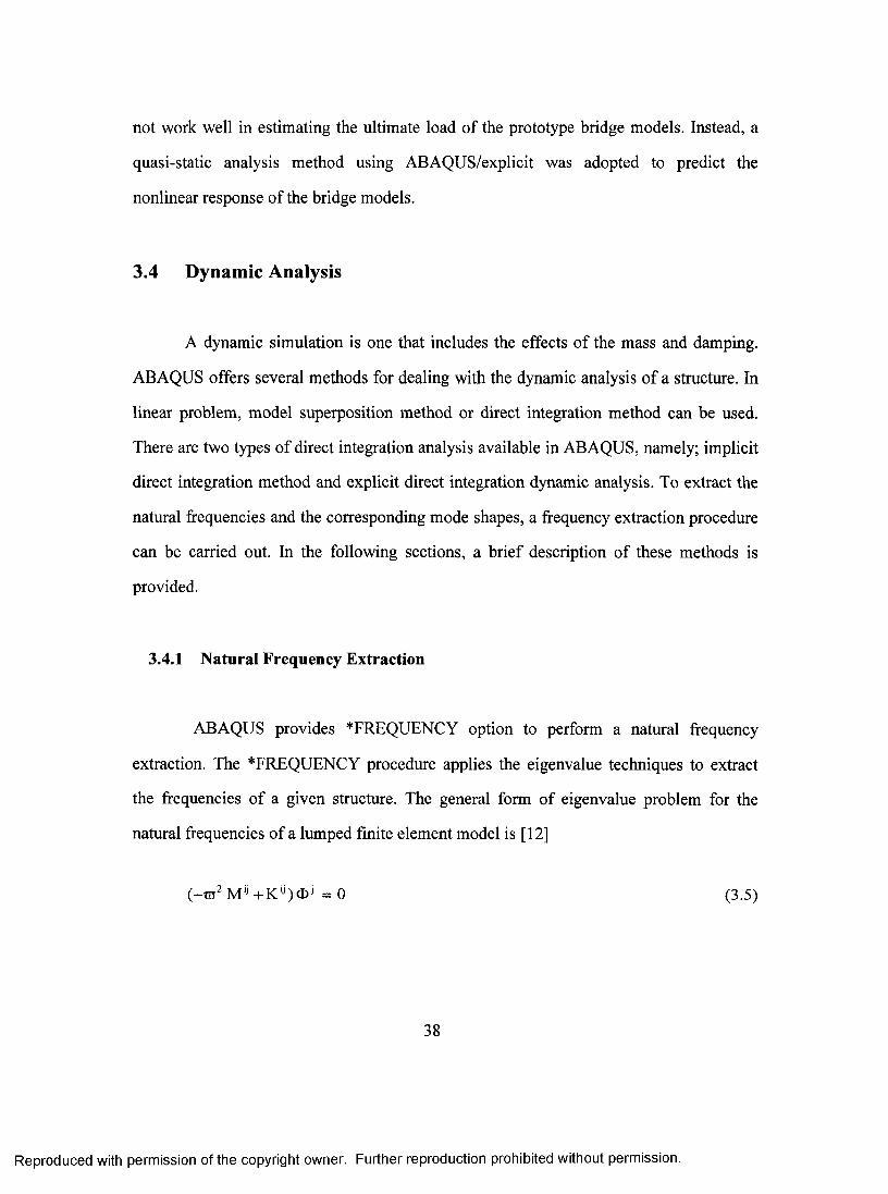
not work well in estimating the ultimate load of the prototype bridge models. Instead, a
quasi-static analysis method using ABAQUS/explicit was adopted to predict the
nonlinear response of the bridge models.
3.4 Dynamic Analysis
A dynamic simulation is one that includes the effects of the mass and damping.
ABAQUS offers several methods for dealing with the dynamic analysis of a structure. In
linear problem, model superposition method or direct integration method can be used.
There are two types of direct integration analysis available in ABAQUS, namely; implicit
direct integration method and explicit direct integration dynamic analysis. To extract the
natural frequencies and the corresponding mode shapes, a frequency extraction procedure
can be carried out. In the following sections, a brief description of these methods is
provided.
3.4.1 Natural Frequency Extraction
ABAQUS provides *FREQUENCY option to perform a natural frequency
extraction. The *FREQUENCY procedure applies the eigenvalue techniques to extract
the frequencies of a given structure. The general form of eigenvalue problem for the
natural frequencies of a lumped finite element model is [1 2 ]
( - r a ^ M y + K ' Q t b j = 0 (3 .5)
38
Reproduced with permission of the copyright owner. Further reproduction prohibited without permission.

where M*-* is the mass matrix (which is symmetric and positive definite) ; K'-" is the
stiffness matrix; is the eigenvector; and i and j are degrees of freedom; co is the circular
frequency.
ABAQUS offers Lanczos and Subspace iteration eigenvalue extraction methods.
The Lanczos method is generally faster when a larger number of eigenmodes is required
for a structure with many degrees of freedom. The subspace iteration may be faster when
only a few eigenvalues are required. ABAQUS extracts eigenvalues until either the
required number of eigenvalues has been extracted or the last frequency extracted exceeds
the maximum frequency of interest. In extracting the required natural frequencies and the
corresponding mode shapes for bridges, Subspace iteration method was adopted in this
work. For this method, ABAQUS automatically calculates the participation factor and the
effective mass for each mode. The eigenvectors are normalized by-default so that the
largest displacement entry in each vector is unity. In the case of torsional modes where
the displacements may be negligible, the eigenvalues are normalized so that the largest
rotation entry in each vector is unity.
3.4.2 Transient Modal Dynamic Analysis
A modal dynamic analysis is performed in ABAQUS by using the *MODAL
DYNAMIC procedure. This method is used to analyze transient linear dynamic problems
using modal superposition; it can only be performed after a frequency extraction
procedure since it predicts the structure’s dynamic response according to the extracted
natural modes of the problem. The method is a very popular dynamic analysis technique
but it has several important limitations. The method is only valid for linear systems and
39
Reproduced with permission of the copyright owner. Further reproduction prohibited without permission.
damping in the system must be proportional. The mode superposition procedure is most
useful when the system response can be accurately estimated by considering only a
relatively small subset of all the vibration modes for the system, which is the case in most
structural systems. Thus, the *MODAL DYNAMIC procedure can be much less
expensive computationally than the dynamic analysis using the direct integration method.
The *MODAL DYNAMIC option provides the time period of the analysis and the time
increment to be used. The *MODAL DAMPING option is often used in conjunction with
a modal dynamic analysis to describe the damping of the system.
Concentrated nodal or distributed pressure or body forces can be applied to the
structure in the modal dynamic analysis. The *AMPLITUDE option can be utilized to
define arbitrary time variation of a load given throughout a step. In order to simulate a
truck moving over a bridge deck, the amplitude of truck load must be specified with time
at each nodal point. The computer program interpolates linearly between these given
values of the time increment in the analysis. The dynamic response of the structure due to
the applied load-time history can be obtained in the form of displacement-, velocity-,
acceleration-, and stress-time histories.
3.4.3 Implicit Direct Integration Method
General linear and nonlinear dynamic responses can be evaluated using the
implicit time integration method. In this method, the equation of motion for a general
system is integrated using a numerical step-by-step procedure. Thus, the system
differential equations are integrated directly in a coupled form, as they exist in the
physical coordinates. Dynamic integration operators are mostly described as implicit or
40
Reproduced with permission of the copyright owner. Further reproduction prohibited without permission.

explicit. The implicit direct integration operator used in ABAQUS is called Hiber-
Hughes-Taylor operator; it is an extension of the trapezoidal rule [70]. Implicit schemes
solve for dynamic quantities at time t+At based not only on values at t, but also on these
same quantities at t+At. In the implicit method, the integration operator matrix must be
inverted and a set of simultaneous dynamic equilibrium equations must be solved at each
time increment. The main advantage of Hilber-Hughes-Taylor operator is that it is
imconditionally stable for linear systems. The direct time increment can be automatieally
provided by ABAQUS or speeified by the user. Artificial damping can be introduced by
the ALPHA parameter on the *DYNAMIC option. The parameter values vary from 0,
which gives no artificial damping, to -0.33, which provides the maximum artifieial
damping available for this operator. At the maximum level ALPHA gives a damping ratio
of about 6 % when time increment is 40% of the period of oscillation of the mode being
studied. Therefore, this artifieial damping is never very substantial for realistic time
increments. The moving loaded truck across the bridge deck can be simulated by using
the *AMPLITUDE option or by writing a subroutine *DLOAD to deseribe the load-time
histories at each nodal point on the bridge deek. A typieal input file for the dynamic
analysis using a user-subroutine is given in Appendix A.
3.5 Explicit Dynamic Analysis
The explicit method is well-suited to solving quasi-static analysis with
complicated nonlinear structural behaviour. The explicit dynamic procedure performs a
large number of small-time increments efficiently. The explicit central difference operator
satisfies the dynamic equilibrium equations at the beginning of the increment, t. Then, the
accelerations calculated at time, t, are used to advance the velocity solution to time t+At/ 2
41
Reproduced with permission of the copyright owner. Further reproduction prohibited without permission.

and the displacement solution to time t+At. The use of diagonal element mass matrices is
the key to the computational efficiency of the explicit procedure, where the inversion of
the mass matrix required at the beginning of the increment is simple to compute. The
central difference operator is conditionally stable. A small amount of damping is
introduced in the analysis to control high frequency oscillations. The time incrementation
scheme in explicit analysis is fully automatic. The central difference method is required to
be integrated at a time step, At, smaller than a critical time step, Atcr- The critical time
step, Atcr, can be evaluated from the mass and stiffness properties of the complete
structure, where Atcr can be obtained as [70]
At„ = i (3.6)7t
where T„ is the smallest period of the finite element assemblage with n degrees of
freedom. In ABAQUS, the stable time increment is given by [70]
At < + ) (3.7)
where is the fraction of critical damping in the mode with the highest frequency. Hence,
the cost of the analysis may be very expensive in cases where the total analysis time is
high.
This method was adopted in predicting the collapse load of the bridge. While this
method is a dynamic analysis method, only the ultimate static load is sought; the bridge
was loaded slowly enough to eliminate any significant inertia effects. The prototype
42
Reproduced with permission of the copyright owner. Further reproduction prohibited without permission.

bridge deck slab was loaded by applying a velocity that increased linearly from 0 to 40
mm/s. Such very low load rate was selected to ensure quasi-static solution. The
computational cost of this solution is relatively high, however, the results obtained from
this method showed good agreement with the experimental findings as described in
Chapter V.
3.6 Finite Element Modelling of Bridge Models
The finite element technique was used to model continuous curved concrete deck-
on multiple steel box girder bridges. Three-dimensional finite element model was
constructed in a way to simulate the actual structural geometry, boundary conditions, and
material properties of the bridge components namely: reinforced concrete deck slab, steel
webs, steel bottom flange, steel top flange, diaphragms, cross bracings, and top chords.
The reinforced concrete slab was fully constrained to the steel top flanges by means of
shear connectors.
In this section, the element types selected for each component, the material
modelling, and the boundary conditions are described. The model presented herein was
verified and substantiated by results gathered from the experimental values from two
continuous composite box girder bridge models tested under several loading cases as
shown in Chapter V.
43
Reproduced with permission of the copyright owner. Further reproduction prohibited without permission.

3.6.1 Material Modelling
The material library in ABAQUS allows the modelling of the material used in the
bridges studied. The bridge slab is made of reinforeed eonerete while the rest of the box
girder is made of steel. In the input file, eaeh material definition starts with a
*MATERIAL option. The material option bloeks define the behaviour of a partieular
material throughout the analysis.
3.6.1.1 Modelling of Steel
In the elastie analysis, only the modulus of elasticity, Poisson’s ratio, and the
material density are required to be given in the input file. The density is used in case of
dynamic analysis or to calculate the gravitation loads of the studied bridges. The
*PLASTIC option must be defined, wherever the plastic behaviour of the steel is needed
in the analysis. Since the steel is assumed to be perfectly plastic, only the yield stress
must be given in the *PLASTIC option. This classical metal plasticity model uses von
Mises yield surface with associated plastic flow for isotropic metal behaviour. The von
Mises surface assumes that the metal yielding is independent of the equivalent stress and
it is used to define isotropic yielding. It is defined by giving the value of the uniaxial yield
stress as a function of uniaxial equivalent plastic strain. The true stress-true strain must be
used in defining the plasticity data in ABAQUS. Figure 3.1 presents the elastic-perfectly-
plastie stress-strain relationship assumed for steel in the finite element analysis.
44
Reproduced with permission of the copyright owner. Further reproduction prohibited without permission.

3.6.1.2 Modelling of Reinforced Concrete
The reinforced concrete bridge deck slab can be modelled in ABAQUS by
defining the concrete model using * CONCRETE option and the reinforcement in the
concrete by the *REBAR option. The ^TENSION STIFFENING option is required in the
concrete model. This option allows for the effects of reinforcement interaction with
concrete to be simulated in a simple manner where the load is transferred aeross the
concrete cracks through the rebar.
3.6.1.3 Concrete Model
The concrete model in ABAQUS is intended to model plain concrete element or
with the *REBAR LAYER option to model reinforced concrete elements. The most
essential aspect of modelling the concrete behaviour is cracking, which dominate the
concrete model under loading. Once the stress in the concrete reaches a failure surfaee,
called crack detection surface, cracks occur. Cracks in the concrete model are
irrecoverable but they may open and close during the calculation. The concrete model
does not track each individual crack. Instead, the model is considered a smeared crack
model by forming constitutive calculations independently at each integration point of the
finite element model. The presenee of cracks is introduced in the calculations by
considering their effect on the stress and material stiffness associated with the integration
point.
In the case of reinforced concrete model, the strain-softening behaviour for
cracked concrete can be identified by using the setting TYPE parameter equal to STRAIN
on the *TENSION STIFFENING option. In the case of the reinforced concrete model, it
45
Reproduced with permission of the copyright owner. Further reproduction prohibited without permission.

is recommended that each element contain a rebar to reduce the mesh sensitivity. The
tension stiffening value must be assumed. It is assumed that strain softening after failure
reduces the stress linearly to zero at a total strain of about 1 0 times the strain at failure.
Figure 3.2 illustrates the simulation of the influence of the rebar in the concrete model
implemented in the finite element model. The failure stress, a “ , occurs at a failure
strain, ef*.
The concrete reveals initially an elastie response when it is loaded in compression.
As a result of increasing the stress in the concrete beyond the elastic region, inelastic
straining takes place and the response of the concrete softens. When the ultimate stress is
reached the material softens such that it can no longer carry any stress. At some point
after inelastistic straining has occurred and the model is unloaded, the reduction in the
model stiffnesses is ignored in the model. If the model is loaded in tension under uniaxial
load, cracks form at a stress corresponding to, typically, 7-10% of the ultimate
compression stress. Figure 3.3 shows that cracking and compression responses of
concrete are integrated in the model by the uniaxial response of a specimen. For the
purpose of developing the model it is assumed that the material loses strength through a
softening mechanism and that this is a dominantly a damage effect in the sense that open
cracks can be represented by loss of elastic stiffness. It is also assumed that cracks are
allowed to close completely if the stress across them becomes compression. In multiaxial
stress states observations can be implemented through the concept of surfaces of failure
and the ultimate strength in the stress space. The computer program defines these surfaces
as shown in Figure 3.4, fitted to experimental data. The *FAILURE RATIOS option can
be used to define the shape of the failure surface. The model is based on the classical
concepts of theory of plasticity.
46
Reproduced with permission of the copyright owner. Further reproduction prohibited without permission.
In ABAQUS/explicit, the brittle cracking model is used for the concrete structure.
The *BR1TTLE CRACKING option is used to define the concrete model. The brittle
cracking model allows removal of elements with *BR1TTLE FAILURE option. In this
model, the postfailure behaviour for direct straining across cracks is modeled with the
^BRITTLE CRACKING option.
3.6.1.4 Rebar Model
In ABAQUS, the *REBAR LAYER option is used to define the reinforcement in
the concrete. The rebars are treated in the model as one-dimensional isoparametric
elements. These elements are superposed on the mesh of the plain concrete elements. The
standard metal plasticity model shown in Figure 3.1 is assumed to deseribe the behaviour
of the rebar material. Adopting this model approach, the concrete behaviour is considered
independently of the rebar. This option can model double layers of the rebar in the
longitudinal direction and double layer of the rebar in the transverse direction. The area of
each rebar, the offset of the mid surface in shell element and the spacing can be defined in
the model. In ABAQUS an equivalent smeared orthotropic layer is assumed. The
equivalent thickness of the smeared layer is equal to the area of the rebar divided by the
rebar’s spaeing. The rebar can be also placed in the radial and tangential directions, as
required in the case of curved deck slabs.
3.6.2 Geometric Modelling
A three-dimensional finite element model was created to simulate each bridge
studied. Three-dimensional shell elements were selected to model the reinforced concrete
47
Reproduced with permission of the copyright owner. Further reproduction prohibited without permission.
deck slab, steel webs, steel bottom flanges, and steel end-diaphragms. For the steel top
flanges, top chords and cross-bracing, three-dimensional beam elements were chosen in
the finite element model. The connections between the reinforced concrete deck slab and
the steel top flanges were idealized using the *MPC option. Figure 3.5 illustrates a typical
idealized cross-section of a bridge.
ABAQUS offers a wide variety of shell elements for stress/displacement analysis.
A four-node doubly curved general-purpose shell element called S4R was adopted in
modelling the required bridge components. The element can idealize either straight or
curved boundaries depending on the node definition. The element has six active degrees
of freedom at each node; three displacements (Ui, U2, U3) and three rotation ((j)i, ^2 , <j)3).
The general-purpose elements are suitable in all loading conditions for thin and thick
shell elements and provide robust and accurate results. The element allows transverse
shear deformation. They use thick shell theory as its shell thickness increases and become
discrete Kirchhoff thin shell element as the thickness decreases. When a shell element is
made of the same material throughout its thickness, the element is considered a thick
element when the thickness is more than 1/15 of a characteristic length on the surface of
the shell. This characteristic length is the span for a static analysis and the wavelength of
a significant natural mode for the dynamic analysis. This element type uses the reduced
integration to form the element stiffness. However, the matrix and distributed loadings
are still integrated exactly. Reduced integration usually provides accurate results and
significantly reduces the computational cost. The shell element accounts for finite
membrane strains and will allow for change in thickness. Figure 3.6 shows a detailed
description of the shell element S4R.
48
Reproduced with permission of the copyright owner. Further reproduction prohibited without permission.
The three-dimensional two-node linear interpolation beam element called B31H
was used to model the steel top flanges, top-chords and cross bracing. The beam element
reduces the problem to one-dimensional problem mathematically and therefore, the
computational time is reduced. The Timoshenko B31H element allows for transverse
shear deformation. The element has two-nodes with six degrees of freedom at each node,
three displacements (Ui, U2, U3) and three rotations ((j)i, (j>2, ^3 ). This hybrid element is
well suited to handle very slender components, where the axial stiffness of the member is
very large compared with its bending stiffness. In this case, the element is considered to
be loaded mainly in tension and compression. The element defines the orientation of the
beam, whether it is straight or curved. Figure 3.7 shows a detailed description of the beam
element chosen for the bridge models.
The *MPC option in ABAQUS allows constraints to be imposed between
different degrees of freedom of the model. The multi-point constraint option was adopted
to simulate the connection between the concrete slab and the steel top flange. This option
is used to ensure full interaction between the concrete deck slab and the steel box girder.
Thus, MFC type is used to model the shear connectors between two nodes. This type is
sorted internally by ABAQUS so that the MFC is imposed by eliminating the degree of
freedom at the first node given. Thus the first node in the MFC option becomes a
dependent node on the last node defined in the option. Therefore, both nodes produce the
same degree of freedom.
49
Reproduced with permission of the copyright owner. Further reproduction prohibited without permission.
3.6.3 Boundary Conditions
There were two different boundary constraints considered in modelling the
continuous curved concrete deck on multiple steel box girder bridges: the roller support
and the binged support. The *BOUNDARY option was used in ABAQUS to prescribe
both boundary conditions for the analysis. The roller support was modeled by releasing
the horizontal movements of the node in the required directions. However, the binged
support was constrained from any horizontal movements. All supports were constrained
in the vertical direction, but allowed to rotate around the support line. In the case of
curved bridge models, the tangential, radial, and vertical support arrangements were
adopted. The support conditions were applied at the lower end nodes of each web, at the
outer and internal support lines, as shown in Figure 3.8.
3.7 Finite Element Analysis of Bridge Models
Various finite element meshes were eonstrueted and compared to select the most
suitable mesh for the linear and nonlinear analyses. In idealizing bridges, mesh
convergence was investigated first, by means of several pilot runs. Figure 3.9 illustrates
the final finite element mesh used in the static and dynamic analyses of twin-box girder
bridges. Two elements on each side of the boxes and four elements between the webs
were used in the transverse direction for all the bridges. In the longitudinal direction, the
total number of elements varied depending upon the span length of the bridge. The
number of elements was 72 for 20-m span bridge, 144 for 40-m span bridge, 432 for 60-
m span bridge, 576 for 80-m span bridge, and 720 for 100-m span bridge. The webs and
the end-diaphragms were simulated using six elements in the vertical direction for all
50
Reproduced with permission of the copyright owner. Further reproduction prohibited without permission.

bridge models. The mesh proved to be adequate for the static and dynamic analyses. The
chosen mesh was quite adequate to accommodate different truck loading cases, as
described in Chapter VI. The total number of elements used to model the bridges varied
from around 4,000 in the case of bridges with span length of 20 m, to 106,000 in the case
of bridges with span length of 100 m. For curved bridge models, the generation of the
elements were in the radial and tangential directions. The aspect ratios of the element
used for the concrete deck slab and the bottom flanges ranged from 1.0 to 1.9 for all
bridge models. The aspect ratios of the shell element for the webs and end-diaphragms
ranged between 1.2 and 2.1 for all the bridge models. However, for bridges with span
length of 20 m, this aspect ratio was 4.
A sensitivity study was conducted to examine the effect of vertical web stiffeners
on the overall structural behaviour of the bridges. The study showed that these stiffeners
had an insignificant influence on the linear response of the bridge structure. Also, it was
established from the pilot runs that the steel reinforcement in the concrete deck slab had
only marginal effects on the bridge elastie response in the static and dynamic analyses.
However, in the nonlinear analysis the effect of the reinforcement was considerable in
predicting the ultimate load for the bridge models. The cross bracing members were
modeled to connect the points at the comer of the box girders. The connecting gusset
plates were ignored. The top chord members were idealized at the same level as the top
steel flanges. The shear connectors were considered to be at the element nodes over the
top steel flanges. The finite element modelling was conducted using a well-established
technique adopted by Sennah [124]. The finite element model was verified using static
equilibrium checks. In addition, the model was substantiated and validated by results
obtained from testing two continuous concrete deck-steel two-box girder bridge models
51
Reproduced with permission of the copyright owner. Further reproduction prohibited without permission.

discussed in Chapter V. The finite element model was then adopted to conduct extensive
parametric studies for static and dynamic responses of continuous curved composite box
girder bridges. Typical input data decks employed in the analysis are given in Appendix
A.
52
Reproduced with permission of the copyright owner. Further reproduction prohibited without permission.
CHAPTER IV
Experimental Study
4.1 Introduction
The presence of continuity and curvature in multi-box girder bridges add
considerably to their complex structural behaviour. Due to torsional moments, stresses
and deformations developed in such bridge members are significant. Experimental studies
can provide design engineers and Specification writers with an insight to their response to
loads. A few experimental studies have been undertaken to verify the elastic response of
box girder bridges. However, experimental investigations on continuous curved concrete
deck on steel multiple box girder bridges at construction phase, service and ultimate load
stages as well as under free vibration conditions are yet unavailable. In this research, an
experimental study has been conducted on two continuous, twin-box girder bridge models
to achieve the following main objectives:
(1) To establish accurate experimental data base and compare it with those
obtained from the finite element analysis.
(2) To investigate the elastic response of continuous curved multi-box
girder bridges at the construction phase and under service loading
conditions.
53
Reproduced with permission of the copyright owner. Further reproduction prohibited without permission.

(3) To determine the free-vibration response of such bridges.
(4) To use the data gathered experimentally from the inelastic structural
response of the bridge models to validate a finite element model
capable of predicting the structural behaviour of the prototype bridges
up to failure.
(5) To determine the collapse load of such bridges and compare the results
to those predicted by the analytical solution.
The experimental program is described in details in this chapter. Bridge models,
geometry, material properties, instrumentation and loading cases are presented. Views of
the model test equipment and test set-up are also presented.
4.2 Description of Bridge Models
In general, full-scale experimental investigation would entail high
expenditures. The availability of suitable testing equipment and space are the important
consideration in choosing suitable length scale factor. Mirza [97] and others have shown
that models erected to scales as small as 1/6 to 1/8 can be reliable, time-saving and
relatively inexpensive. Based on the previous considerations, a length scale factor 1/8 was
selected. The aim of this experimental study is to compare its results with the ones
obtained from the finite element method for the same model with the same linear scale
length. Thus, for practical reasons a larger linear scale length was used for the thickness
54
Reproduced with permission of the copyright owner. Further reproduction prohibited without permission.
of the steel box plates and reinforced concrete deck, in order to avoid difficulties in the
fabrication process.
The concrete deck was constructed without the curbs for simplification and to
match the analytical model used. Care was taken and special procedures were followed to
minimize the amount of possible deformation of the steel box section during fabrication
as a result of welding. The depth of the steel box section was maintained constant at 150
mm throughout for both the straight and curved bridge models.
Two continuous two-box girder bridge models were constructed. The first model
was a straight, while the second one was curved in plan with span-to-radius of curvature
ratio of 1. Figures 4.1 and 4.2 show plans for the straight and curved bridge models,
respectively. The thickness of all steel plates used to construct the steel box sections was
3 mm. Each box girder consisted of a bottom flange 7300-mm long and 270-mm wide,
two top flanges each 7300-mm long and 47-mm wide and two webs each 7300-mm long
and 144-mm deep. At the end support lines and the interior support line only, diaphragms
with access holes were welded inside the boxes, while cross bracing were provided
between the boxes. Also, cross bracings were used inside and between the boxes in both
models at equal intervals between the support lines. Cross bracing members were made of
20 X 3 m m rectangular cross section. It should be noted that these cross members were
installed in the radial direction in the curved model at equal intervals. C-channel section
was used as shear connectors to provide full interaction between the concrete deck and
the steel box section. Shear connectors with a length of 25-mm were placed at 100-mm
intervals, being in the radial direction. Four layers of steel reinforcement wires were
placed in the longitudinal and transverse directions, in the case of the straight bridge
55
Reproduced with permission of the copyright owner. Further reproduction prohibited without permission.
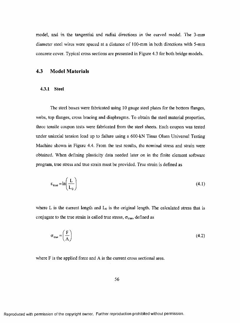
model, and in the tangential and radial directions in the curved model. The 3-mm
diameter steel wires were spaced at a distance of 100-mm in both directions with 5-mm
eonerete cover. Typical cross sections are presented in Figure 4.3 for both bridge models.
4.3 Model Materials
4.3.1 Steel
The steel boxes were fabricated using 10 gauge steel plates for the bottom flanges,
webs, top flanges, cross bracing and diaphragms. To obtain the steel material properties,
three tensile coupon tests were fabricated from the steel sheets. Each coupon was tested
under uniaxial tension load up to failure using a 600-kN Tinus Olsen Universal Testing
Machine shovra in Figure 4.4. From the test results, the nominal stress and strain were
obtained. When defining plasticity data needed later on in the finite element software
program, true stress and true strain must be provided. True strain is defined as
^ true (4.1)
where L is the current length and Lo is the original length. The calculated stress that is
conjugate to the true strain is called true stress, atme, defined as
^true Ix Jwhere F is the applied force and A is the current cross sectional area.
56
Reproduced with permission of the copyright owner. Further reproduction prohibited without permission.
Nominal strain can be expressed as
L - L o LSno m in a l = “ j— ^ = ~ ~ 1 ( 4 .3 )
L q L q
The relationship between true stress and nominal stress is formed by considering
the following equation:
Lo Ao = L A (4.4)
Carrying out the necessary substitutions provides the relationship between true
strain and nominal strain and true stress and nominal stress, as follows:
^ t ru e ~ n o m in a l ) ( 4 -5 )
^ t r u e “ ^ n o m i n a l ( ^ " ^ ^ n o m i n a l ) ( 4 -6 )
The average relationship between the true stress and true strain for the steel used
to build the box girders is depicted in Figure 4.5.
4.3.2 Concrete
Ready mix concrete was donated by CBM Company for the experimental
program. Smooth limestone 10 mm was used in the concrete mixture with 125-mm
slump. Water-cement ratio and aggregate-cement ratio were selected to obtain a nominal
compressive strength, f c = 40 MPa.
57
Reproduced with permission of the copyright owner. Further reproduction prohibited without permission.

Four standard cylinders 100 x 200 mm and four standard cylinders 150 x 300 mm
were sampled concurrently with the casting of the concrete slab. The cylinders were
placed in the same condition as the concrete deck slab. The cylinders and the concrete
slab were cured for at least two weeks under the same room temperature. All cylindrical
specimens were tested under uniaxial compressive load using the 1350 kN Riehle
Compression Testing Machine, as shown in Figure 4.6. Mechanical Dial gauges were
installed on the concrete specimen to measure displacement. The average strength as well
as Young’s moduli of elasticity of the concrete samples are listed in Table 4.1 and a
typical stress-strain relationship is presented in Figure 4.7.
4.3.3 Steel Wire Reinforcement
Three-millimetre diameter steel wires were used as steel reinforcement at the top
and the bottom of the concrete deck in the longitudinal and transverse directions. Three
specimens were tested under uniaxial tension load up to failure. After obtaining the load-
displacement relationship from the laboratory tests, the average true stress-true strain
results were calculated and are shown in Figure 4.8. The yield strength and modulus of
elasticity were found to be 800 MPa and 208 GPa, respectively.
4.3.4 Shear Connectors
To ensure full interaction between the concrete slab deck and the steel section, 25-
mm deep, 10-mm flange width chaimel-sections were used as shear connectors. The
channel section was cut into pieces 25 mm in length. Marks on the top flanges of box
girders at 100 mm were drawn to weld the shear connectors to the top flanges. Three
coupons were cut from the channel section and the average true stress-true strain
58
Reproduced with permission of the copyright owner. Further reproduction prohibited without permission.

relationship is presented in Figure 4.9. The shear connectors were positioned on all top
flanges and along the entire length of both bridge models. A view of the shear connectors
welded to the steel top flanges is shown in Figure 4.10.
4.4 Model Construction
4.4.1 Fabrication of Open Steel Section
Steel boxes forming both bridge models were fabricated using the same steel
plates for the bottom flanges, webs, top flanges, cross bracing and diaphragms. Top
flanges and webs were first formed from the flat steel sheets. Then, the webs were
clamped in position with the top flanges and tack welded at discrete locations to reduce
the amount of possible distortion during the welding process. To minimize the heat
generation during the welding process, a medium-heat welding machine was used.
To make it possible to weld the cross bracing and the diaphragm inside the steel
boxes, they were welded to the top flange-web members first before welding the bottom
flange of the box. Then, bottom flanges cut from flat steel sheets were clamped to the
webs in position. Spot welds were used to ensure the right dimension and to stabilize the
cross-section during the welding process. Shear connectors were placed and then welded,
as illustrated in Figure 4.10, on the top flanges and the fabricated open steel box girder
was completed. Continuous welding was provided at the interface of channel shear
connectors. Finally, each box girder was carried and positioned in its testing place on the
supports. A view of the straight bridge model after welding is shown in Figure 4.11. The
two box girders were then connected using the cross bracing members between the boxes.
59
Reproduced with permission of the copyright owner. Further reproduction prohibited without permission.

4.4.2 Model Supports
The interior support in both models was placed in the centre of the structural rigid
portal frame available in the structural laboratory. The bridge model support conditions
were designed to simulate the interior bearings as a hinged support and the outer bearings
as roller supports. In the case of the curved bridge model, the outer bearings were released
in the tangential direction. However, at the interior support the bridge model was
prevented from movement in the tangential direction by welding a steel rod just beside
the roller underneath each web. At each support line, the bridge model was tied down
using a tie-down system to prevent the bridge models from uplift movements.
4.4.3 Concrete Formwork
After placing the steel box girders in the testing position under the laboratory
structural frame, the concrete formwork was prepared. Twelve-millimetre plywood sheets
were installed under the steel box girders and supported to the laboratory floor by 100 x
100 mm wooden struts. To form the slab overhang and the slab between the steel box
girders, strips of styrofoam sheets 5 and 10 mm thick were used on the top of the plywood
to form the bottom surface of the concrete deck. One hundred-millimetre of styrofoam
sheets were installed inside the steel boxes with intermediate supports made of small
pieces of these sheets. It should be noted that the styrofoam strips inside the boxes could
not have been removed after easting the eonerete. However, due to their negligible
stiffness, they would not affect the structural performance of the model. Styrofoam
sheets, 40 mm thick, were cut to form the edge of the concrete slab. In the case of the
curved bridge model, small pieces of styrofoam were used to support a very thin flexible
60
Reproduced with permission of the copyright owner. Further reproduction prohibited without permission.
wood strip of 40 mm depth, to obtain a well-formed curved edge of the concrete slab. A
view of the formwork for the curved bridge model is presented in Figure 4.12.
4.4.4 Reinforcing Steel Wire
Two meshes of reinforcing steel wires were placed at a distance of 100 mm in
both directions near the top and bottom surface of the concrete slab. To ensure the
stability of the wire mesh during casting the concrete slab, the wires in the transverse
direction were first placed and tied to the bottom of the shear connectors. On the top of
the transverse wires, the longitudinal wires were put on place and held to the transverse
wires. Figures 4.13 and 4.14 show the wire meshes in straight and curved bridge models,
respectively. Due to the flexibility of the steel wire, it was possible to form the steel wires
in the tangential direction in the curved bridge model easily.
Similar procedures were followed to place the top steel wire layer. First, the
transverse wires (the radial in the curved bridge model) were held to the top of the shear
connectors and then the longitudinal wires (the tangential in the curved bridge model)
were placed on top of them. Small pieces of wires were used to ensure a proper cover at
the bottom of the concrete deck and were observed to make sure that they were not
displaced during casting the concrete.
4.4.5 Casting the Concrete Deck
Casting the concrete deck required extreme care in order to prevent the flexible
vsdre meshes or the styrofoam from displacing. Concrete was carried from the mixer to the
end of the bridge and carefully shovelled onto the bridge model. The concrete was
61
Reproduced with permission of the copyright owner. Further reproduction prohibited without permission.
compacted manually, where the thickness of the concrete deck was only 40 mm. Then,
the concrete surface was finished with a wooden screed from one end of the bridge and
continued to the other end. To ensure a well-finished surface a final troweling with a steel
screed was made. Later, the concrete was moist-cured for two weeks along with the
concrete cylinders sampled at the time of casting the concrete deck slab, as shown in
Figure 4.15.
4.5 Instrumentation
4.5.1 Strain Gauges
Strain gauges were installed at three cross-sections along the bridge model,
namely: The middle of the first span, the interior support, and the middle of the second
span. Electrical strain gauges type N11-FA-10-350-11 (Showa Co., Ltd) were used at
thirty-two different locations along the bridge model. The length of each strain gauge was
10 mm, with a resistance of 350 + 0.3 % ohms. The gauge faetor varied from 2.14 to 2.15
± 1 %. All the steel strain gauges were placed in the longitudinal direction of the bridge
models. The installed strain gauges on the bottom flange of a steel box at the mid-span
are shown in Figure 4.16.
Eight concrete strain gauges of type N2A-06-20CBW-350 (Showa Co., Ltd) were
used on eaeh bridge model. The length of the concrete strain gauge was 50 mm, with a
resistance of 350. + 0.3% ohms. The gauge faetor was 2.10 ± 0.5% for all concrete strain
gauges used in both models. Three concrete strain gauges were positioned on the concrete
deck at the middle of the first span, three over the interior support and two at the middle
62
Reproduced with permission of the copyright owner. Further reproduction prohibited without permission.
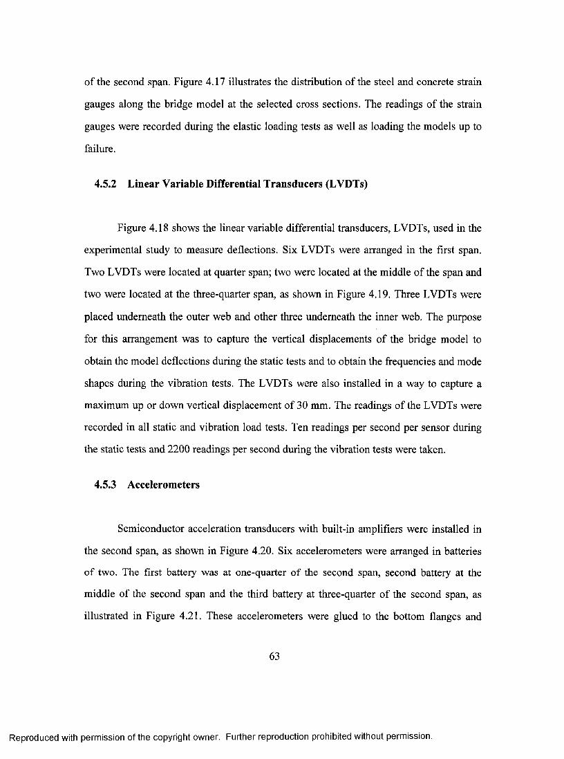
of the second span. Figure 4.17 illustrates the distribution of the steel and concrete strain
gauges along the bridge model at the selected cross sections. The readings of the strain
gauges were recorded during the elastic loading tests as well as loading the models up to
failure.
4.5.2 Linear Variable Differential Transducers (LVDTs)
Figure 4.18 shows the linear variable differential transducers, LVDTs, used in the
experimental study to measure deflections. Six LVDTs were arranged in the first span.
Two LVDTs were located at quarter span; two were located at the middle of the span and
two were located at the three-quarter span, as shown in Figure 4.19. Three LVDTs were
placed underneath the outer web and other three underneath the inner web. The purpose
for this arrangement was to capture the vertical displacements of the bridge model to
obtain the model deflections during the static tests and to obtain the frequencies and mode
shapes during the vibration tests. The LVDTs were also installed in a way to capture a
maximum up or down vertical displacement of 30 mm. The readings of the LVDTs were
recorded in all static and vibration load tests. Ten readings per second per sensor during
the static tests and 2200 readings per second during the vibration tests were taken.
4.5.3 Accelerometers
Semiconductor acceleration transducers with built-in amplifiers were installed in
the second span, as shown in Figure 4.20. Six accelerometers were arranged in batteries
of two. The first battery was at one-quarter of the second span, second battery at the
middle of the second span and the third battery at three-quarter of the second span, as
illustrated in Figure 4.21. These accelerometers were glued to the bottom flanges and
63
Reproduced with permission of the copyright owner. Further reproduction prohibited without permission.
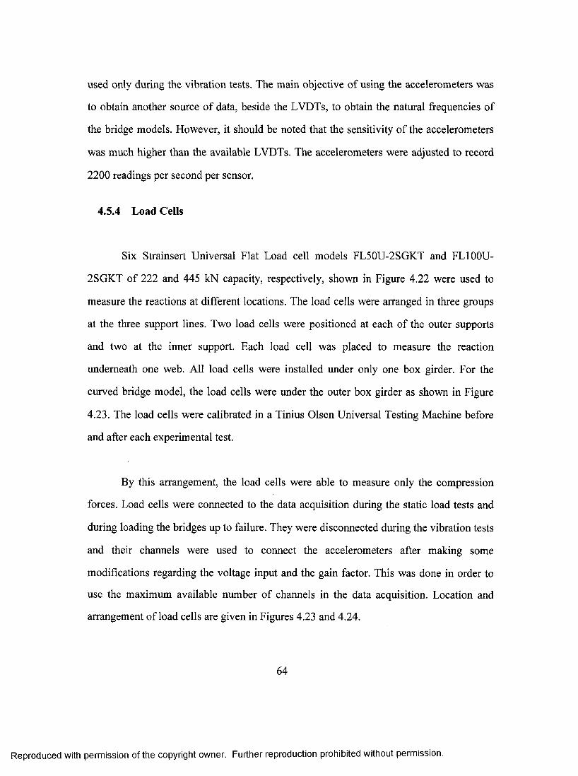
used only during the vibration tests. The main objective of using the accelerometers was
to obtain another source of data, beside the LVDTs, to obtain the natural frequencies of
the bridge models. However, it should be noted that the sensitivity of the accelerometers
was much higher than the available LVDTs. The accelerometers were adjusted to record
2200 readings per second per sensor.
4.5.4 Load Cells
Six Strainsert Universal Flat Load cell models FL50U-2SGKT and FLIOOU-
2SGKT of 222 and 445 kN capacity, respectively, shown in Figure 4.22 were used to
measure the reactions at different locations. The load cells were arranged in three groups
at the three support lines. Two load cells were positioned at each of the outer supports
and two at the irmer support. Each load cell was placed to measure the reaction
underneath one web. All load cells were installed under only one box girder. For the
curved bridge model, the load cells were under the outer box girder as shown in Figure
4.23. The load cells were calibrated in a Tinius Olsen Universal Testing Machine before
and after each experimental test.
By this arrangement, the load cells were able to measure only the compression
forces. Load cells were cormected to the data acquisition during the static load tests and
during loading the bridges up to failure. They were disconnected during the vibration tests
and their channels were used to connect the accelerometers after making some
modifications regarding the voltage input and the gain factor. This was done in order to
use the maximum available number of channels in the data acquisition. Location and
arrangement of load cells are given in Figures 4.23 and 4.24.
64
Reproduced with permission of the copyright owner. Further reproduction prohibited without permission.

4.5.5 Data Acquisition System
The available seven cards installed in the MEG AD AC 3000 series data
acquisition unit were effectively used to obtain as much data as possible from the
experimental investigations. Eaeh card contains eight channels that can be adjusted to a
certain power input and gain factors that depend on the sensors connected to that card.
The first four cards, thirty-two channels, were connected to steel strain gauges and the
fifth one was connected to the concrete strain gauges. One card was used to read the data
from the linear variable differential transducers, LVDTs. The last available card was used
for the load cells in the static load tests (and the accelerometers in the vibration tests).
Test Control Software program (TCS) was installed in the MEGADEC to capture
the data from the sensors and then save and export it in ASCII format for further analysis.
During the static tests, the reading rate of the all sensors was 10 readings per second per
sensor. However, in an attempt to maintain high accuracy in the vibration tests, where the
required readings were for only the sensors connected to the LVDTs and the
accelerometers, it was possible to increase the rate of reading to 2200 readings per second
per sensor. A view of the data acquisition unit beside the straight bridge model along with
electrical cormections to all the sensors is shown in Figure 4.25.
4.5.6 Hydraulic Jacks
Three hydraulic jacks were utilized to perform the static and vibration tests. Two
hydraulic jacks were used in the static load tests where each jack had a capacity of 890
kN. One hydraulic jack was supported on the transverse beam of the structural frame to
allow jack movement in the transverse direction only. The second jack was supported on
65
Reproduced with permission of the copyright owner. Further reproduction prohibited without permission.
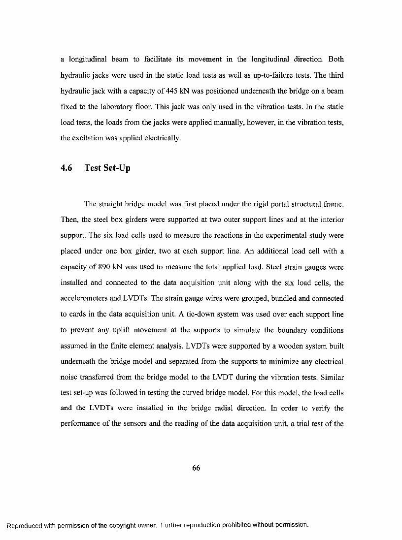
a longitudinal beam to facilitate its movement in the longitudinal direction. Both
hydraulic jacks were used in the static load tests as well as up-to-failure tests. The third
hydraulic jack with a capacity of 445 kN was positioned underneath the bridge on a beam
fixed to the laboratory floor. This jack was only used in the vibration tests. In the static
load tests, the loads from the jacks were applied manually, however, in the vibration tests,
the excitation was applied electrically.
4.6 Test Set-Up
The straight bridge model was first placed under the rigid portal structural frame.
Then, the steel box girders were supported at two outer support lines and at the interior
support. The six load cells used to measure the reactions in the experimental study were
placed under one box girder, two at each support line. An additional load cell with a
capacity of 890 kN was used to measure the total applied load. Steel strain gauges were
installed and cormected to the data acquisition unit along with the six load cells, the
accelerometers and LVDTs. The strain gauge wires were grouped, bundled and cormected
to cards in the data acquisition unit. A tie-down system was used over each support line
to prevent any uplift movement at the supports to simulate the boundary conditions
assumed in the finite element analysis. LVDTs were supported by a wooden system built
underneath the bridge model and separated from the supports to minimize any electrical
noise transferred from the bridge model to the LVDT during the vibration tests. Similar
test set-up was followed in testing the curved bridge model. For this model, the load cells
and the LVDTs were installed in the bridge radial direction. In order to verify the
performance of the sensors and the reading of the data acquisition unit, a trial test of the
66
Reproduced with permission of the copyright owner. Further reproduction prohibited without permission.
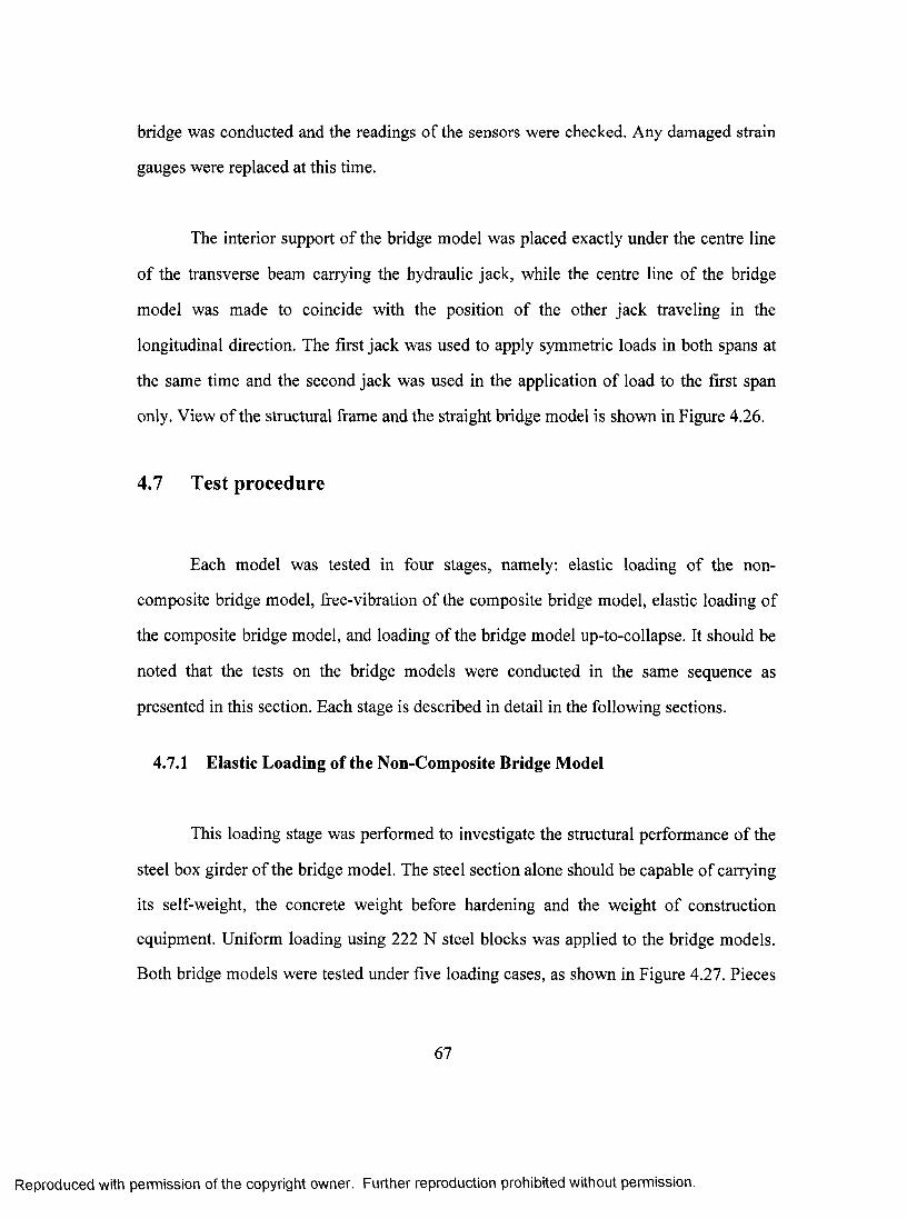
bridge was conducted and the readings of the sensors were checked. Any damaged strain
gauges were replaced at this time.
The interior support of the bridge model was placed exactly under the centre line
of the transverse beam carrying the hydraulic jack, while the centre line of the bridge
model was made to coincide with the position of the other jack traveling in the
longitudinal direction. The first jack was used to apply symmetric loads in both spans at
the same time and the second jack was used in the application of load to the first span
only. View of the structural frame and the straight bridge model is shown in Figure 4.26.
4.7 Test procedure
Each model was tested in four stages, namely: elastic loading of the non
composite bridge model, ffee-vibration of the composite bridge model, elastic loading of
the composite bridge model, and loading of the bridge model up-to-collapse. It should be
noted that the tests on the bridge models were conducted in the same sequence as
presented in this section. Each stage is described in detail in the following sections.
4.7.1 Elastic Loading of the Non-Composite Bridge Model
This loading stage was performed to investigate the structural performance of the
steel box girder of the bridge model. The steel section alone should be capable of carrying
its self-weight, the concrete weight before hardening and the weight of construction
equipment. Uniform loading using 222 N steel blocks was applied to the bridge models.
Both bridge models were tested under five loading cases, as shown in Figure 4.27. Pieces
67
Reproduced with permission of the copyright owner. Further reproduction prohibited without permission.
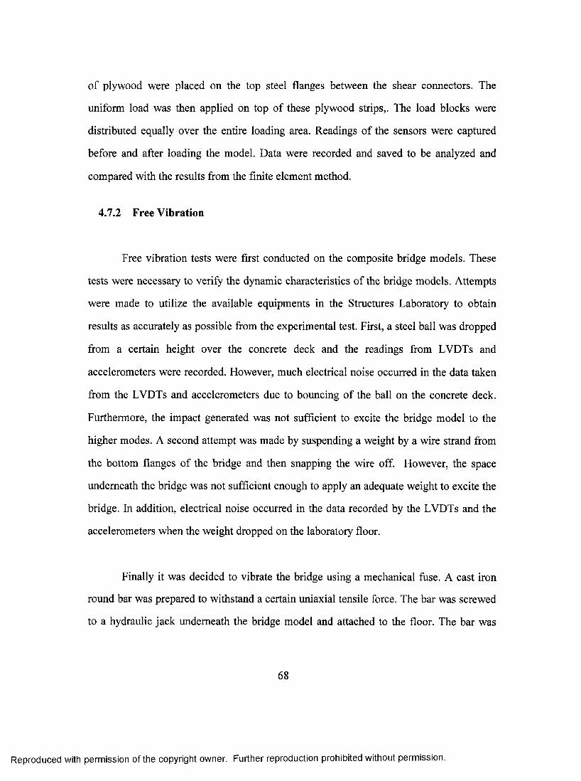
of plywood were placed on the top steel flanges between the shear connectors. The
uniform load was then applied on top of these plywood strips,. The load blocks were
distributed equally over the entire loading area. Readings of the sensors were captured
before and after loading the model. Data were recorded and saved to be analyzed and
compared with the results from the finite element method.
4.7.2 Free Vibration
Free vibration tests were first conducted on the composite bridge models. These
tests were necessary to verify the dynamic characteristics of the bridge models. Attempts
were made to utilize the available equipments in the Structures Laboratory to obtain
results as accurately as possible from the experimental test. First, a steel ball was dropped
from a certain height over the concrete deck and the readings from LVDTs and
accelerometers were recorded. However, much electrical noise occurred in the data taken
from the LVDTs and accelerometers due to bouncing of the ball on the concrete deck.
Furthermore, the impact generated was not sufficient to excite the bridge model to the
higher modes. A second attempt was made by suspending a weight by a wire strand from
the bottom flanges of the bridge and then snapping the wire off. However, the space
underneath the bridge was not sufficient enough to apply an adequate weight to excite the
bridge. In addition, electrical noise occurred in the data recorded by the LVDTs and the
accelerometers when the weight dropped on the laboratory floor.
Finally it was decided to vibrate the bridge using a mechanical fuse. A cast iron
round bar was prepared to withstand a certain uniaxial tensile force. The bar was screwed
to a hydraulic jack underneath the bridge model and attached to the floor. The bar was
68
Reproduced with permission of the copyright owner. Further reproduction prohibited without permission.
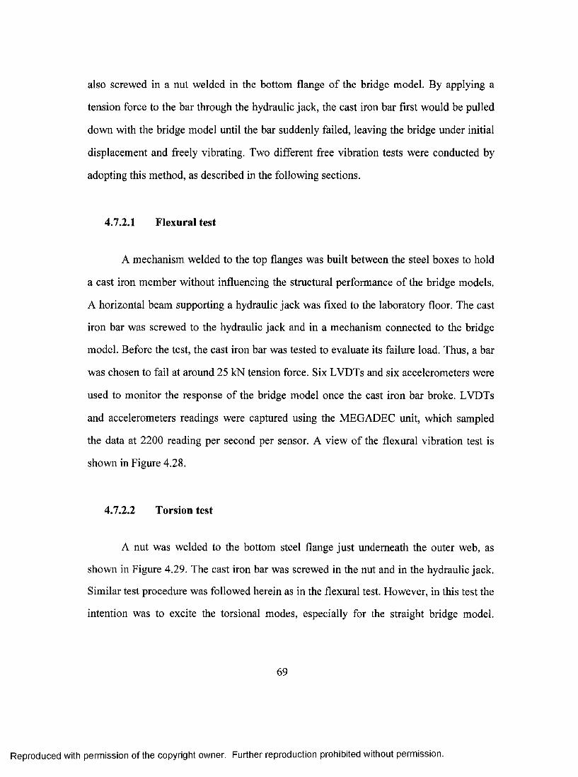
also screwed in a nut welded in the bottom flange of the bridge model. By applying a
tension force to the bar through the hydraulic jack, the cast iron bar first would be pulled
down with the bridge model until the bar suddenly failed, leaving the bridge under initial
displacement and freely vibrating. Two different free vibration tests were conducted by
adopting this method, as described in the following sections.
4.7.2.1 Flexural test
A mechanism welded to the top flanges was built between the steel boxes to hold
a cast iron member without influencing the structural performance of the bridge models.
A horizontal beam supporting a hydraulic jack was fixed to the laboratory floor. The cast
iron bar was screwed to the hydraulic jack and in a mechanism connected to the bridge
model. Before the test, the cast iron bar was tested to evaluate its failure load. Thus, a bar
was chosen to fail at around 25 kN tension force. Six LVDTs and six accelerometers were
used to monitor the response of the bridge model once the cast iron bar broke. LVDTs
and accelerometers readings were captured using the MEGADEC unit, which sampled
the data at 2200 reading per second per sensor. A view of the flexural vibration test is
shovm in Figure 4.28.
4.7.2.2 Torsion test
A nut was welded to the bottom steel flange just underneath the outer web, as
shovm in Figure 4.29. The cast iron bar was screwed in the nut and in the hydraulic jack.
Similar test procedure was followed herein as in the flexural test. However, in this test the
intention was to excite the torsional modes, especially for the straight bridge model.
69
Reproduced with permission of the copyright owner. Further reproduction prohibited without permission.
Recording the readings of LVDTs and accelerometers was started just before turning the
hydraulic jack on and stopped after the vibrations of the model died out.
4.7.3 Elastic Loading of the Composite Bridge Models
The objective here of the experimental test was to investigate the elastic structural
behaviour of the bridge models. Since this test was conducted after the free vibration
tests, some cracks were observed over the interior support due to series of attempts to
vibrate the bridge models. Various loading conditions were applied to the bridge model:
four cases in the case of the straight bridge model and six cases in the case of the curved
bridge model. The straight bridge model was subjected to the following loading cases:
(1) Two concentrated loads, one over each web of one box, were
applied over the webs of one box girder at 0.4 of the span from the
outer support line. View of this loading case is shown in Figure
4.30.
(2) Four concentrated loads, one over each web, were applied at 0.4 of
the span from the outer support line. View of this loading case is
shown in Figure 4.31.
(3) Four concentrated loads, two in each span and one over each web
of one box, were applied at 0.6 of the span from the outer support
line. View of this loading case is shown in Figure 4.32.
70
Reproduced with permission of the copyright owner. Further reproduction prohibited without permission.
(4) Eight concentrated loads, one over each web, four loads per span,
applied at 0.6 of the span from the outer support line. View of this
loading case is shown in Figure 4.33.
Loadings cases (1) and (2) were intended to simulate partially and fully loaded
lanes to obtain the maximum stresses in the positive moment region. However, loadings
cases (3) and (4) were intended to represent partially and fully loaded lanes to obtain the
maximum stresses in the negative moment region. For all the loading cases, the
concentrated loads were always applied over the webs to prevent any possibility of
punching the 40 mm concrete deck. For all the loading cases, the applied load was
increased slowly until each load reached a value of 15 kN.
Six static tests were conducted on the curved bridge model as follows:
(1) Two concentrated loads, one over each web of the outer box, were
applied at 0.4 of the span from the outer support line. View of this
loading case is shown in Figure 4.34.
(2) Two concentrated loads, one over each web of the irmer box, were
applied at 0.4 of the span from the outer support line. View of this
loading case is shown in Figure 4.35.
(3) Four concentrated loads, one over each web of each box, were applied
at 0.4 of the span from the outer support line. View of this loading case
is shown in Figure 4.36.
71
Reproduced with permission of the copyright owner. Further reproduction prohibited without permission.

(4) Two concentrated loads in each span, one over each web of the outer
box, were applied at 0.6 of the span from the outer support line. View
of this loading case is shown in Figure 4.37.
(5) Two concentrated loads in each span, one over each web of the inner
box, were applied at a distance of 0.6 the span from the outer support
line. View of this loading case is shown in Figure 4.38.
(6) Four concentrated loads in each span, one over each web, were applied
at 0.6 of the span from the outer support line. View of this loading case
is shown in Figure 4.39.
In all load cases for the curved bridge model, the loads were positioned over the
webs in the radial direction. All LVDTs, strain gauges and load cells readings data were
recorded and analyzed.
4.7.4 Loading of Bridge Models Up-to-CoIlapse
This static load test was conducted to obtain the structural response under
overloads as well as to determine the collapse load for each bridge model. The straight
bridge model was subjected to eight concentrated loads at a distance of 2145 mm from
the outer support line. The curved bridge model was subjected to eight concentrated loads
at a distance of 2150 mm, measured on the central line arc of the bridge model from the
outer support line. Under this loading case, a plastic hinge was expected to develop at the
interior support. Increasing the loads resulted in complete failure of the structure when
72
Reproduced with permission of the copyright owner. Further reproduction prohibited without permission.

two other plastic hinges developed near the mid spans. The loads were increased slowly
to have sufficient time to trace the cracks on the concrete deck.
The readings of the LVDTs, strain gauges and load cells were recorded during the
entire loading time history until failure. All loads wee applied over the webs to prevent
any possibility of punching the concrete slab before reaching the overall collapse load of
the bridge model. Significant deflections were observed near the mid spans associated
with severe web bucking of the steel section at the interior support. The test was then
terminated for safety reasons and the load was released slowly.
73
Reproduced with permission of the copyright owner. Further reproduction prohibited without permission.

CHAPTER V
Model Validation
5.1 Introduction
Experimental details of the bridge models were presented in the previous ehapter.
Since the main objective of the experimental program was to validate and substantiate the
finite element model used in the static and dynamic analyses of such bridges, comparison
between the experimental results and the results obtained from the finite element solution
is required. Results recorded in the experimental study were compared with those
obtained from finite element analysis using the commercial software “ABAQUS”,
suitably modified. To idealize the continuous composite two-box bridges models, the
modelling techniques presented in Chapter III were employed for both the straight and
curved bridge models. The results from the static load cases presented in this ehapter
include: deflections, longitudinal strains, support reactions, and collapse loads of the
bridge models. The results obtained from the free-vibration tests were also analyzed and
presented.
74
Reproduced with permission of the copyright owner. Further reproduction prohibited without permission.
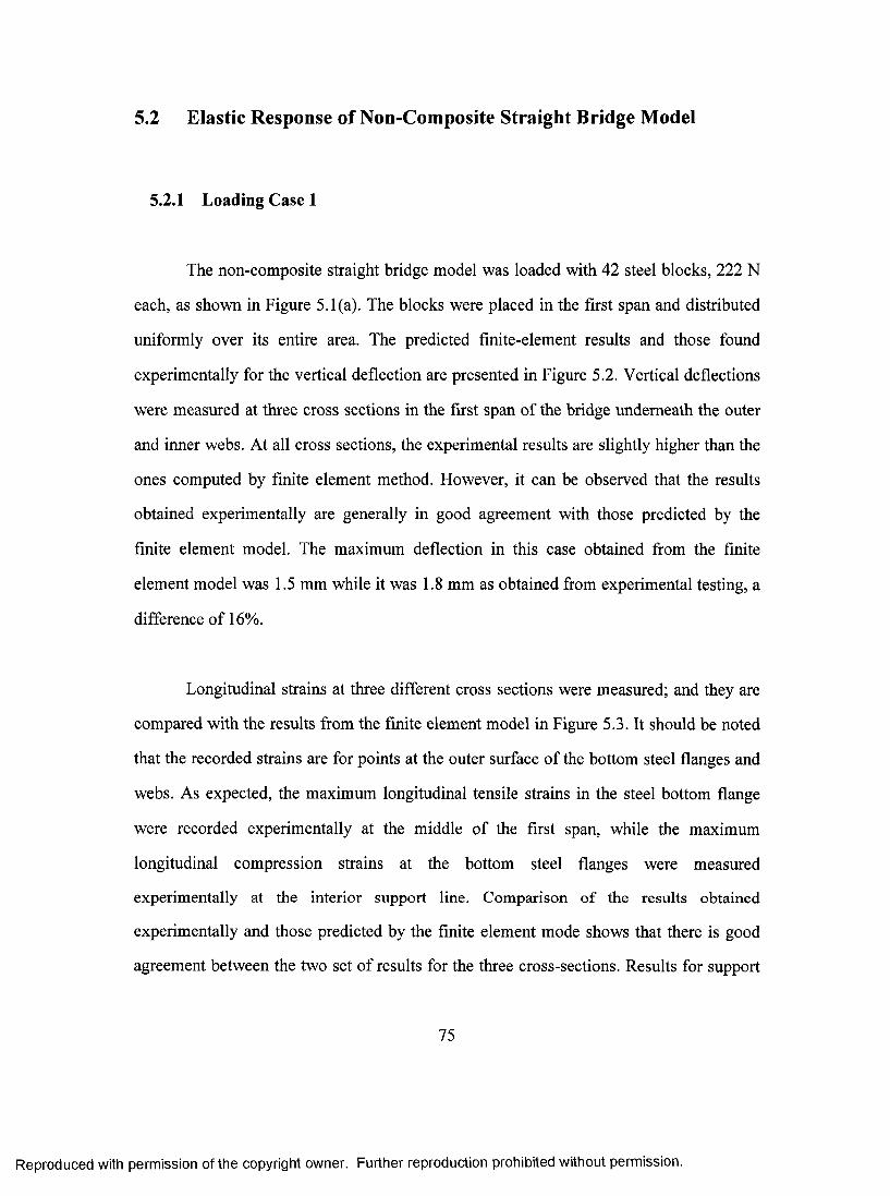
5.2 Elastic Response of Non-Composite Straight Bridge Model
5.2.1 Loading Case 1
The non-composite straight bridge model was loaded with 42 steel blocks, 222 N
each, as shown in Figure 5.1(a). The blocks were placed in the first span and distributed
uniformly over its entire area. The predicted finite-element results and those found
experimentally for the vertical deflection are presented in Figure 5.2. Vertical deflections
were measured at three cross sections in the first span of the bridge underneath the outer
and inner webs. At all cross sections, the experimental results are slightly higher than the
ones computed by finite element method. However, it can be observed that the results
obtained experimentally are generally in good agreement with those predicted by the
finite element model. The maximum deflection in this case obtained from the finite
element model was 1.5 mm while it was 1.8 mm as obtained from experimental testing, a
difference of 16%.
Longitudinal strains at three different cross sections were measured; and they are
compared with the results from the finite element model in Figure 5.3. It should be noted
that the recorded strains are for points at the outer surface of the bottom steel flanges and
webs. As expected, the maximum longitudinal tensile strains in the steel bottom flange
were recorded experimentally at the middle of the first span, while the maximum
longitudinal compression strains at the bottom steel flanges were measured
experimentally at the interior support line. Comparison o f the results obtained
experimentally and those predicted by the finite element mode shows that there is good
agreement between the two set of results for the three cross-sections. Results for support
75
Reproduced with permission of the copyright owner. Further reproduction prohibited without permission.
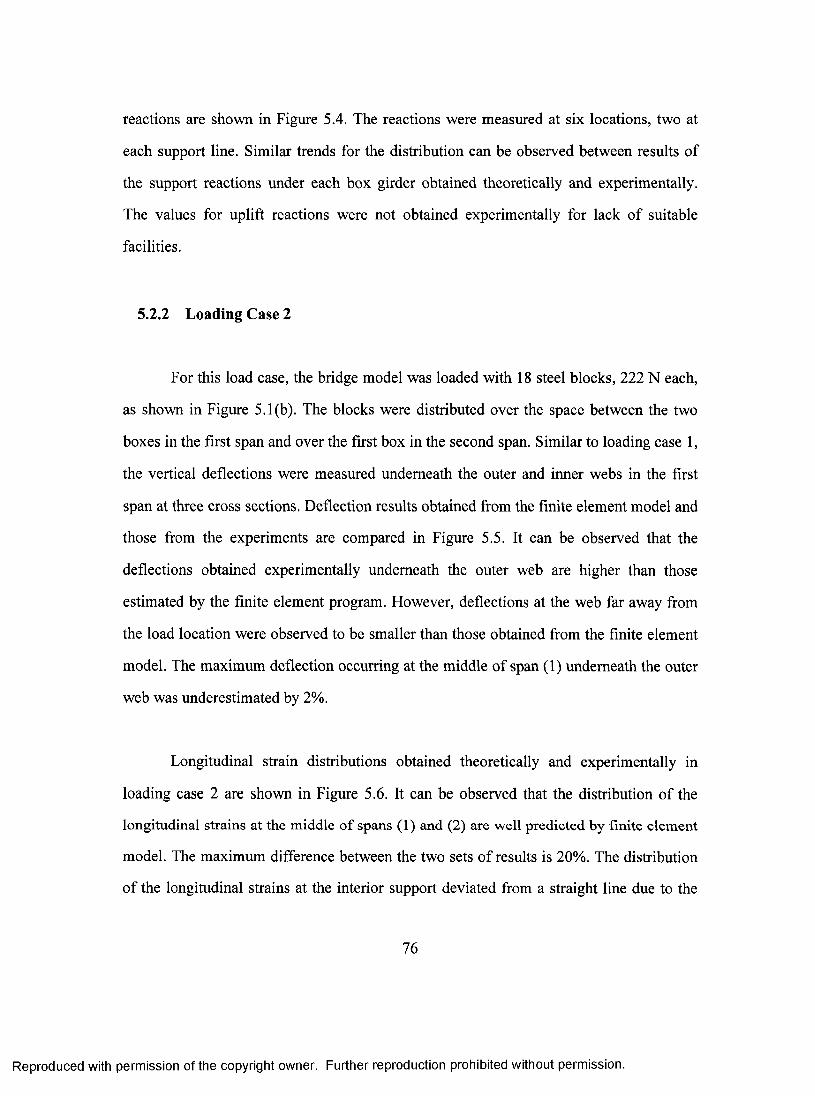
reactions are shown in Figure 5.4. The reactions were measured at six locations, two at
each support line. Similar trends for the distribution can be observed between results of
the support reactions under each box girder obtained theoretically and experimentally.
The values for uplift reactions were not obtained experimentally for lack of suitable
facilities.
5.2.2 Loading Case 2
For this load case, the bridge model was loaded with 18 steel blocks, 222 N each,
as shown in Figure 5.1(b). The blocks were distributed over the space between the two
boxes in the first span and over the first box in the second span. Similar to loading case 1,
the vertical deflections were measured underneath the outer and inner webs in the first
span at three cross sections. Deflection results obtained from the finite element model and
those from the experiments are compared in Figure 5.5. It can be observed that the
deflections obtained experimentally underneath the outer web are higher than those
estimated by the finite element program. However, deflections at the web far away from
the load location were observed to be smaller than those obtained from the finite element
model. The maximum deflection occurring at the middle of span (1) underneath the outer
web was underestimated by 2%.
Longitudinal strain distributions obtained theoretically and experimentally in
loading case 2 are showm in Figure 5.6. It can be observed that the distribution of the
longitudinal strains at the middle o f spans (1) and (2) are well predicted by finite element
model. The maximum difference between the two sets of results is 20%. The distribution
of the longitudinal strains at the interior support deviated from a straight line due to the
76
Reproduced with permission of the copyright owner. Further reproduction prohibited without permission.

localized effect of the boundary conditions. Support reactions due to loading case 2 are
presented in Figure 5.7. It can be observed that the maximum support reaction occurred at
the interior support, as expected. This loading case did not produce uplift at any of the
support points. It can also be observed that total reactions underneath each support line
obtained theoretically and experimentally are in good agreement. Yet, the experimentally
obtained transverse reaction distribution is somewhat different from that estimated by the
finite element model, the maximum difference being under 25%.
5.2.3 Loading Case 3
Unlike the previous loading cases, there was no distributed load between the
boxes. The loading case 3 was antisymmetric in both spans and only over each box, as
shown in Figure 5.1(c). Deflection plots for this loading case are shown in Figure 5.8.
Results obtained by the finite element model and from tests are compared. As can be
seen, the results predicted by the finite element model agree quite well with those
obtained from the experimental study. The maximum deflection developed under the
outer web in the mid-span 1.
Figure 5.9 compares the longitudinal strains for loading case 3 at three different
cross sections. It can be seen that the experimental results of the distribution of the
longitudinal strains along these cross sections at the mid-span locations can be well
predicted by the finite element model. However, it was no surprise to observe some
fluctuations in the results at the interior support, where the locations o f the strain gauges
were close to the supports. The predicted and measured support reactions for loading case
77
Reproduced with permission of the copyright owner. Further reproduction prohibited without permission.
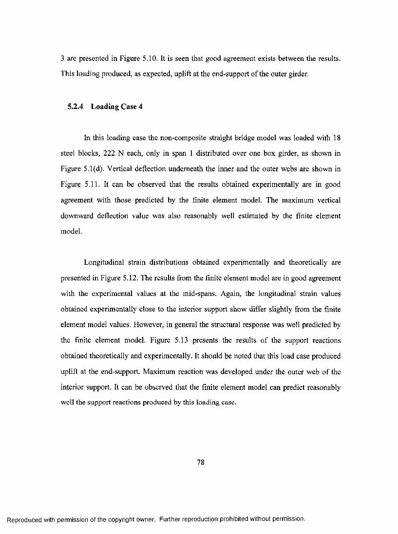
3 are presented in Figure 5.10. It is seen that good agreement exists between the results.
This loading produced, as expected, uplift at the end-support of the outer girder.
5.2.4 Loading Case 4
In this loading case the non-composite straight bridge model was loaded with 18
steel blocks, 222 N each, only in span 1 distributed over one box girder, as shown in
Figure 5.1(d). Vertical deflection underneath the inner and the outer webs are shown in
Figure 5.11. It can be observed that the results obtained experimentally are in good
agreement with those predicted by the finite element model. The maximum vertical
downward deflection value was also reasonably well estimated by the finite element
model.
Longitudinal strain distributions obtained experimentally and theoretically are
presented in Figure 5.12. The results from the finite element model are in good agreement
with the experimental values at the mid-spans. Again, the longitudinal strain values
obtained experimentally close to the interior support show differ slightly from the finite
element model values. However, in general the structural response was well predicted by
the finite element model. Figure 5.13 presents the results of the support reactions
obtained theoretically and experimentally. It should be noted that this load case produced
uplift at the end-support. Maximum reaction was developed under the outer web of the
interior support. It can be observed that the finite element model can predict reasonably
well the support reactions produced by this loading case.
78
Reproduced with permission of the copyright owner. Further reproduction prohibited without permission.
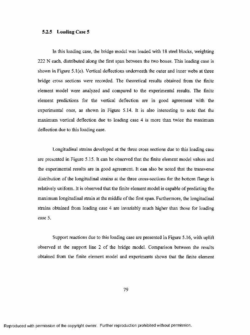
5.2.5 Loading Case 5
In this loading case, the bridge model was loaded with 18 steel blocks, weighting
222 N each, distributed along the first span between the two boxes. This loading case is
shown in Figure 5.1(e). Vertical deflections underneath the outer and inner webs at three
bridge cross sections were recorded. The theoretical results obtained from the finite
element model were analyzed and compared to the experimental results. The finite
element predictions for the vertical deflection are in good agreement with the
experimental ones, as shown in Figure 5.14. It is also interesting to note that the
maximum vertical deflection due to loading case 4 is more than twice the maximum
deflection due to this loading case.
Longitudinal strains developed at the three cross sections due to this loading case
are presented in Figure 5.15. It can be observed that the finite element model values and
the experimental results are in good agreement. It can also be noted that the transverse
distribution of the longitudinal strains at the three cross-sections for the bottom flange is
relatively uniform. It is observed that the finite element model is capable of predicting the
maximum longitudinal strain at the middle of the first span. Furthermore, the longitudinal
strains obtained from loading case 4 are invariably much higher than those for loading
case 5.
Support reactions due to this loading case are presented in Figure 5.16, with uplift
observed at the support line 2 of the bridge model. Comparison between the results
obtained from the finite element model and experiments shows that the finite element
79
Reproduced with permission of the copyright owner. Further reproduction prohibited without permission.
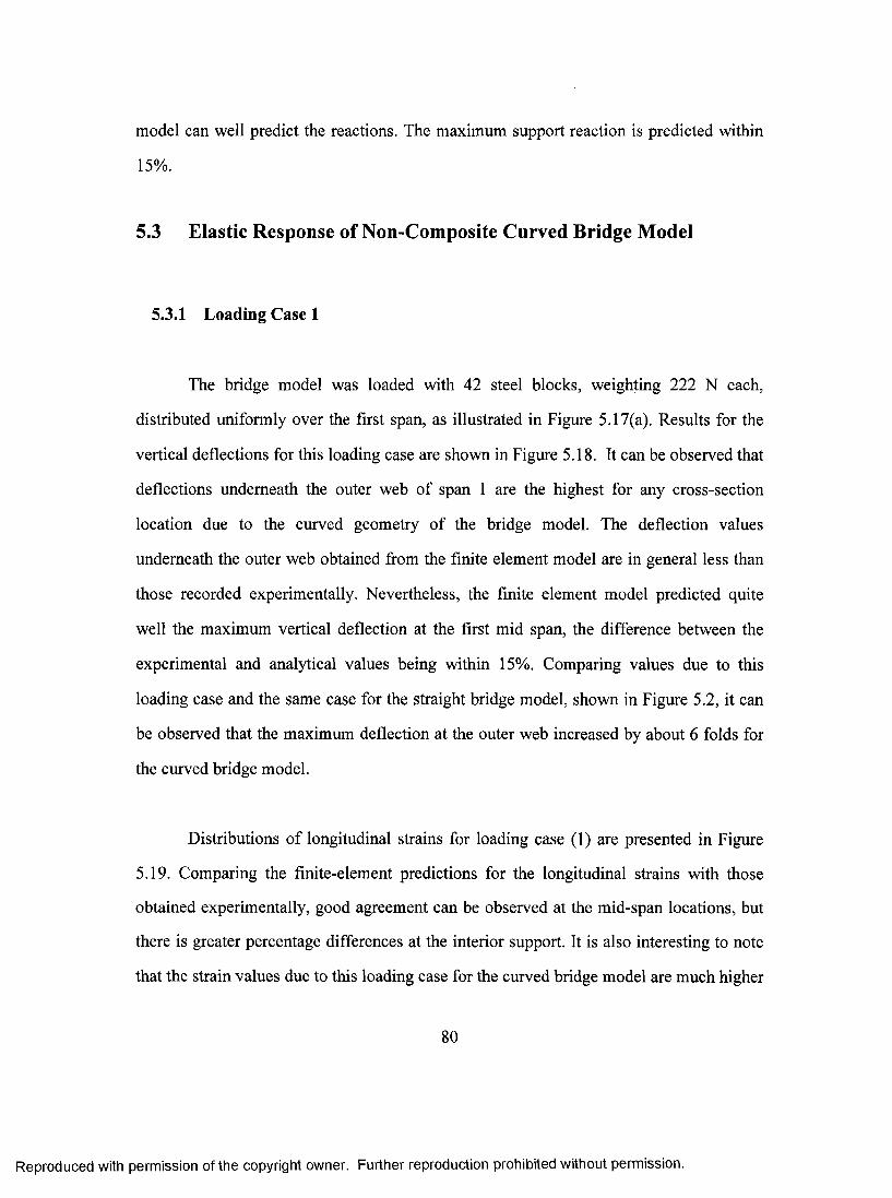
model can well predict the reactions. The maximum support reaction is predicted within
15%.
5.3 Elastic Response of Non-Composite Curved Bridge Model
5.3.1 Loading Case 1
The bridge model was loaded with 42 steel blocks, weighting 222 N each,
distributed uniformly over the first span, as illustrated in Figure 5.17(a). Results for the
vertical deflections for this loading case are shown in Figure 5.18. It can be observed that
deflections underneath the outer web of span 1 are the highest for any cross-section
location due to the curved geometry of the bridge model. The deflection values
underneath the outer web obtained from the finite element model are in general less than
those recorded experimentally. Nevertheless, the finite element model predicted quite
well the maximum vertical defiection at the first mid span, the difference between the
experimental and analytical values being within 15%. Comparing values due to this
loading case and the same case for the straight bridge model, shown in Figure 5.2, it can
be observed that the maximum deflection at the outer web increased by about 6 folds for
the curved bridge model.
Distributions of longitudinal strains for loading case (1) are presented in Figure
5.19. Comparing the finite-element predictions for the longitudinal strains with those
obtained experimentally, good agreement can be observed at the mid-span locations, but
there is greater percentage differences at the interior support. It is also interesting to note
that the strain values due to this loading case for the curved bridge model are much higher
80
Reproduced with permission of the copyright owner. Further reproduction prohibited without permission.
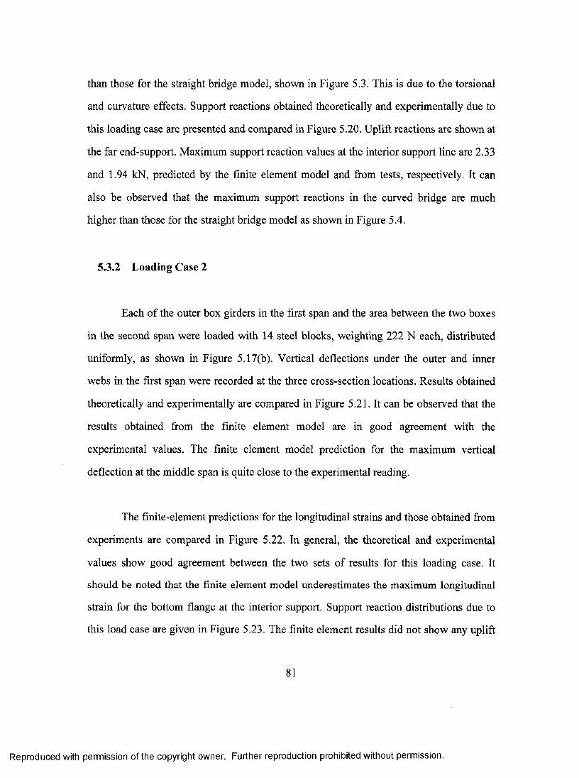
than those for the straight bridge model, shown in Figure 5.3. This is due to the torsional
and curvature effects. Support reactions obtained theoretically and experimentally due to
this loading case are presented and compared in Figure 5.20. Uplift reactions are shown at
the far end-support. Maximum support reaction values at the interior support line are 2.33
and 1.94 kN, predicted by the finite element model and from tests, respeetively. It ean
also be observed that the maximum support reactions in the curved bridge are much
higher than those for the straight bridge model as shown in Figure 5.4.
5.3.2 Loading Case 2
Each of the outer box girders in the first span and the area between the two boxes
in the second span were loaded with 14 steel blocks, weighting 222 N each, distributed
uniformly, as shown in Figure 5.17(b). Vertical deflections under the outer and irmer
webs in the first span were recorded at the three cross-section locations. Results obtained
theoretically and experimentally are compared in Figure 5.21. It can be observed that the
results obtained from the finite element model are in good agreement with the
experimental values. The finite element model prediction for the maximum vertieal
deflection at the middle span is quite elose to the experimental reading.
The finite-element predictions for the longitudinal strains and those obtained from
experiments are compared in Figure 5.22. In general, the theoretical and experimental
values show good agreement between the two sets of results for this loading ease. It
should be noted that the finite element model underestimates the maximum longitudinal
strain for the bottom flange at the interior support. Support reaction distributions due to
this load case are given in Figure 5.23. The finite element results did not show any uplift
81
Reproduced with permission of the copyright owner. Further reproduction prohibited without permission.
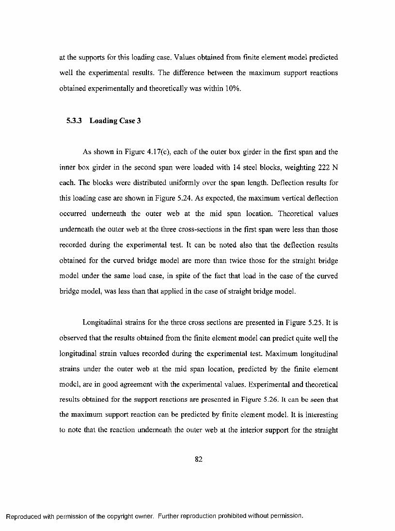
at the supports for this loading case. Values obtained from finite element model predicted
well the experimental results. The difference between the maximum support reactions
obtained experimentally and theoretically was within 10%.
5.3.3 Loading Case 3
As shown in Figure 4.17(c), each of the outer box girder in the first span and the
inner box girder in the second span were loaded with 14 steel blocks, weighting 222 N
each. The blocks were distributed uniformly over the span length. Deflection results for
this loading case are shown in Figure 5.24. As expected, the maximum vertical deflection
occurred underneath the outer web at the mid span location. Theoretical values
underneath the outer web at the three cross-sections in the first span were less than those
recorded during the experimental test. It can be noted also that the deflection results
obtained for the curved bridge model are more than twice those for the straight bridge
model under the same load case, in spite of the fact that load in the case of the curved
bridge model, was less than that applied in the case of straight bridge model.
Longitudinal strains for the three cross sections are presented in Figure 5.25. It is
observed that the results obtained from the finite element model can predict quite well the
longitudinal strain values recorded during the experimental test. Maximum longitudinal
strains under the outer web at the mid span location, predicted by the finite element
model, are in good agreement with the experimental values. Experimental and theoretical
results obtained for the support reactions are presented in Figure 5.26. It can be seen that
the maximum support reaction can be predicted by finite element model. It is interesting
to note that the reaction underneath the outer web at the interior support for the straight
82
Reproduced with permission of the copyright owner. Further reproduction prohibited without permission.
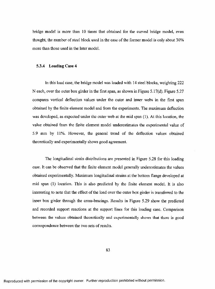
bridge model is more than 10 times that obtained for the cnrved bridge model, even
thought, the number of steel block used in the case of the former model is only about 30%
more than those used in the later model.
5.3.4 Loading Case 4
In this load case, the bridge model was loaded with 14 steel blocks, weighting 222
N each, over the outer box girder in the first span, as shown in Figure 5.17(d). Figure 5.27
compares vertical deflection values under the outer and irmer webs in the first span
obtained by the finite element model and from the experiments. The maximum deflection
was developed, as expected under the outer web at the mid span (1). At this location, the
value obtained from the finite element model underestimates the experimental value of
5.9 mm by 11%. However, the general trend of the deflection values obtained
theoretically and experimentally shows good agreement.
The longitudinal strain distributions are presented in Figure 5.28 for this loading
case. It can be observed that the finite element model generally underestimates the values
obtained experimentally. Maximum longitudinal strains at the bottom flange developed at
mid span (1) location. This is also predicted by the finite element model. It is also
interesting to note that the effect of the load over the outer box girder is transferred to the
inner box girder through the cross-bracings. Results in Figure 5.29 show the predicted
and recorded support reactions at the support lines for this loading case. Comparison
between the values obtained theoretically and experimentally shows that there is good
correspondence between the two sets of results.
83
Reproduced with permission of the copyright owner. Further reproduction prohibited without permission.
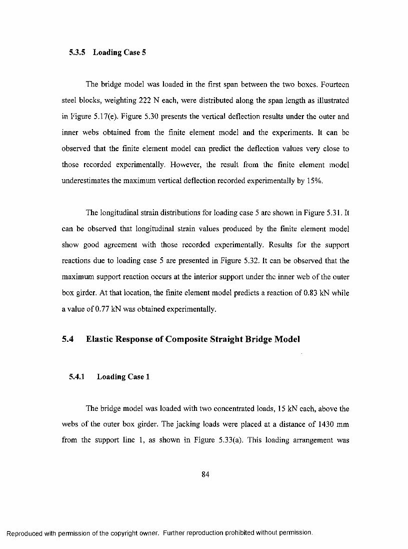
5.3.5 Loading Case 5
The bridge model was loaded in the first span between the two boxes. Fourteen
steel blocks, weighting 222 N each, were distributed along the span length as illustrated
in Figure 5.17(e). Figure 5.30 presents the vertical deflection results under the outer and
inner webs obtained from the finite element model and the experiments. It can be
observed that the finite element model can predict the deflection values very close to
those recorded experimentally. However, the result from the finite element model
underestimates the maximum vertical deflection recorded experimentally by 15%.
The longitudinal strain distributions for loading case 5 are shown in Figure 5.31. It
can be observed that longitudinal strain values produced by the finite element model
show good agreement with those recorded experimentally. Results for the support
reactions due to loading case 5 are presented in Figure 5.32. It can be observed that the
maximum support reaction occurs at the interior support under the inner web of the outer
box girder. At that location, the finite element model predicts a reaction of 0.83 kN while
a value of 0.77 kN was obtained experimentally.
5.4 Elastic Response of Composite Straight Bridge Mode!
5.4.1 Loading Case 1
The bridge model was loaded with two concentrated loads, 15 kN each, above the
webs of the outer box girder. The jacking loads were placed at a distance of 1430 mm
from the support line 1, as shown in Figure 5.33(a). This loading arrangement was
84
Reproduced with permission of the copyright owner. Further reproduction prohibited without permission.
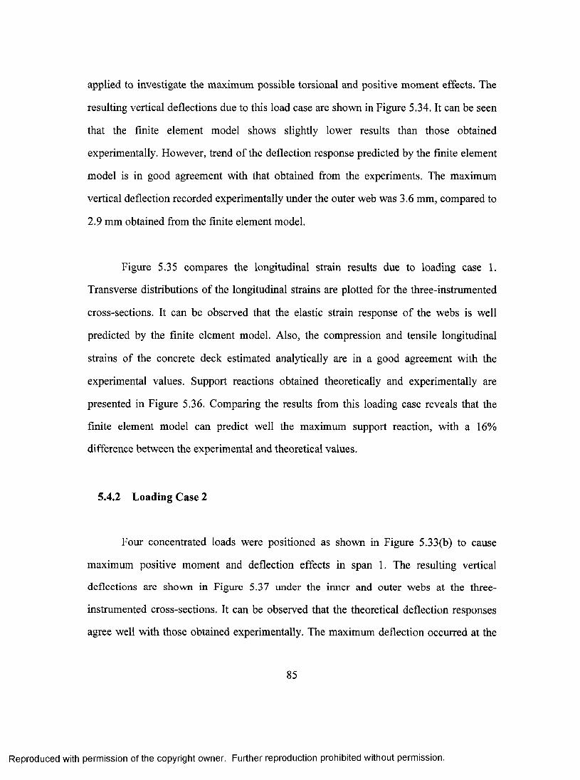
applied to investigate the maximum possible torsional and positive moment effects. The
resulting vertical deflections due to this load case are shovm in Figure 5.34. It can be seen
that the finite element model shows slightly lower results than those obtained
experimentally. However, trend of the deflection response predicted by the finite element
model is in good agreement with that obtained from the experiments. The maximum
vertical deflection recorded experimentally under the outer web was 3.6 mm, compared to
2.9 mm obtained from the finite element model.
Figure 5.35 compares the longitudinal strain results due to loading case 1.
Transverse distributions of the longitudinal strains are plotted for the three-instrumented
cross-sections. It can be observed that the elastic strain response of the webs is well
predicted by the finite element model. Also, the compression and tensile longitudinal
strains of the concrete deck estimated analytically are in a good agreement with the
experimental values. Support reactions obtained theoretically and experimentally are
presented in Figure 5.36. Comparing the results from this loading case reveals that the
finite element model can predict well the maximum support reaction, with a 16%
difference between the experimental and theoretical values.
5.4.2 Loading Case 2
Four coneentrated loads were positioned as shown in Figure 5.33(b) to cause
maximum positive moment and deflection effects in span 1. The resulting vertical
deflections are shown in Figure 5.37 under the inner and outer webs at the three-
instrumented eross-seetions. It can be observed that the theoretieal deflection responses
agree well with those obtained experimentally. The maximum deflection occurred at the
85
Reproduced with permission of the copyright owner. Further reproduction prohibited without permission.
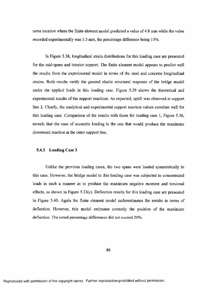
same location where the finite element model predicted a value of 4.8 mm while the value
recorded experimentally was 5.3 mm, the percentage difference being 13%.
In Figure 5.38, longitudinal strain distributions for this loading case are presented
for the mid-spans and interior support. The finite element model appears to predict well
the results from the experimental model in terms of the steel and concrete longitudinal
strains. Both results verify the general elastic structural response of the bridge model
under the applied loads in this loading case. Figure 5.39 shows the theoretical and
experimental results of the support reactions. As expected, uplift was observed at support
line 2. Clearly, the analytical and experimental support reaction values correlate well for
this loading case. Comparison of the results with those for loading case 1, Figure 5.36,
reveals that the case of eccentric loading is the one that would produce the maximum
downward reaction at the outer support line.
5.4.3 Loading Case 3
Unlike the previous loading cases, the two spans were loaded symmetrically in
this case. However, the bridge model in this loading case was subjected to concentrated
loads in such a manner as to produce the maximum negative moment and torsional
effects, as shown in Figure 5.33(c). Deflection results for this loading case are presented
in Figure 5.40. Again the finite element model underestimates the results in terms of
deflection. However, this model estimates correctly the position of the maximum
deflection. The noted percentage differences did not exceed 20%.
86
Reproduced with permission of the copyright owner. Further reproduction prohibited without permission.
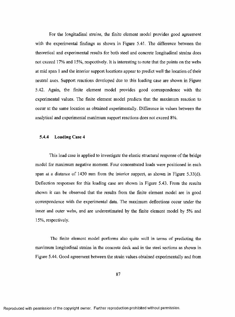
For the longitudinal strains, the finite element model provides good agreement
with the experimental findings as shown in Figure 5.41. The difference between the
theoretical and experimental results for both steel and concrete longitudinal strains does
not exceed 17% and 15%, respectively. It is interesting to note that the points on the webs
at mid span 1 and the interior support locations appear to predict well the location of their
neutral axes. Support reactions developed due to this loading case are shown in Figure
5.42. Again, the finite element model provides good correspondence with the
experimental values. The finite element model predicts that the maximum reaction to
occur at the same location as obtained experimentally. Difference in values between the
analytical and experimental maximum support reactions does not exceed 8%.
5.4.4 Loading Case 4
This load case is applied to investigate the elastic structural response of the bridge
model for maximum negative moment. Four concentrated loads were positioned in each
span at a distance of 1430 mm from the interior support, as shown in Figure 5.33(d).
Deflection responses for this loading case are shown in Figure 5.43. From the results
shown it can be observed that the results from the finite element model are in good
correspondence with the experimental data. The maximum deflections occur under the
inner and outer webs, and are underestimated by the finite element model by 5% and
15%, respectively.
The finite element model performs also quite well in terms of predicting the
maximum longitudinal strains in the concrete deck and in the steel sections as shown in
Figure 5.44. Good agreement between the strain values obtained experimentally and from
87
Reproduced with permission of the copyright owner. Further reproduction prohibited without permission.
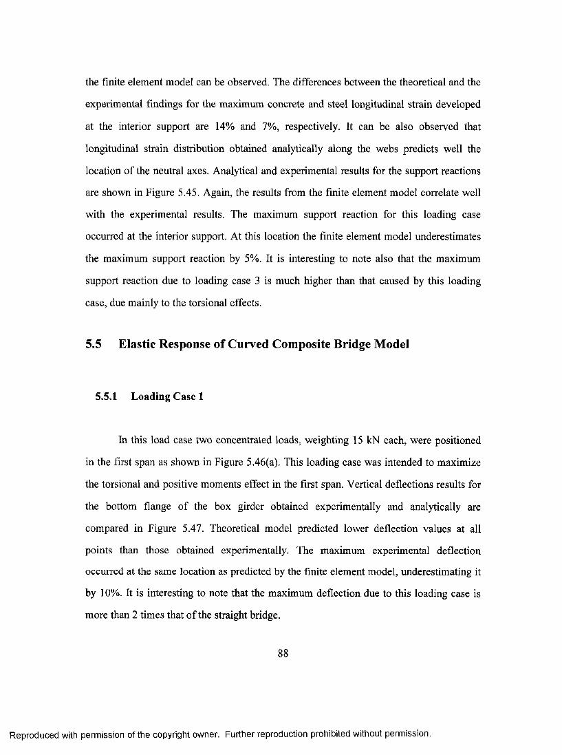
the finite element model can be observed. The differences between the theoretical and the
experimental findings for the maximum concrete and steel longitudinal strain developed
at the interior support are 14% and 7%, respectively. It can be also observed that
longitudinal strain distribution obtained analytically along the webs predicts well the
location of the neutral axes. Analytical and experimental results for the support reactions
are shown in Figure 5.45. Again, the results from the finite element model correlate well
with the experimental results. The maximum support reaction for this loading case
occurred at the interior support. At this location the finite element model underestimates
the maximum support reaction by 5%. It is interesting to note also that the maximum
support reaction due to loading case 3 is much higher than that caused by this loading
case, due mainly to the torsional effects.
5.5 Elastic Response of Curved Composite Bridge Mode!
5.5.1 Loading Case 1
In this load case two concentrated loads, weighting 15 kN each, were positioned
in the first span as shown in Figure 5.46(a). This loading case was intended to maximize
the torsional and positive moments effect in the first span. Vertical deflections results for
the bottom flange of the box girder obtained experimentally and analytically are
compared in Figure 5.47. Theoretical model predicted lower deflection values at all
points than those obtained experimentally. The maximum experimental deflection
occurred at the same location as predicted by the finite element model, underestimating it
by 10%. It is interesting to note that the maximum deflection due to this loading case is
more than 2 times that of the straight bridge.
88
Reproduced with permission of the copyright owner. Further reproduction prohibited without permission.

Comparison of the analytical and experimental longitudinal strains distributions is
shown in Figure 5.48. It is clear that the finite element model can predict reasonably well
the results. It can also be noted that the maximum longitudinal strain due to this loading
case is higher than that for the straight bridge model. Results in Figure 5.49 show the
analytical and experimental support reactions due to loading case 1. Again, good
agreement between the experimental and the theoretical results ean be seen. Maximum
support reaetion values at the interior support are 7.52 kN and 8.63 kN from the finite
element model and experimental model, respectively. It can be observed that maximum
support reaction for the curved model is higher than the one for the straight model.
5.5.2 Loading Case 2
This load case is similar to the previous load case. However, the inner box girder
was loaded instead of the outer box girder, as shown in Figure 5.46(b). Deflections
calculated from the finite element model and the experimental findings are compared in
Figure 5.50. The results show that the maximum deflection occurs at mid-span 1 under
the outer web. Again, the finite element model underestimates the deflection results at all
points. Maximum deflection values predicted by this model and from the experimental
study are 3.1 mm and 3.2 mm, respectively. Obviously, this loading case produces lower
values in terms of deflection than loading case 1.
Results in Figure 5.51 show the calculated and measured longitudinal strains at
various instrumented cross-sections. It is observed that the transverse longitudinal strain
distributions at all cross-section predicted by the finite element model are in good
agreement with those obtained experimentally. It is also noted that the maximum
89
Reproduced with permission of the copyright owner. Further reproduction prohibited without permission.

longitudinal strain at the interior support developed from this loading case is much lower
than those obtained from loading case 1. Support reaction values are compared and
shown in Figure 5.52. Maximum support reaction was observed along support line 1.
Comparison between theoretical and experimental support reactions shows that there is a
good correlation between the two results. Uplift is shown to develop at support line 2.
However, this was not recorded experimentally.
5.5.3 Loading Case 3
Four concentrated loads were positioned in span 1 as shown in Figure 5.46(c).
Maximum positive moment effects accompanied with torsional effects were produced
due to this loading case. Deflection results are shown for the three instrumented cross-
sections in Figure 5.53. The finite element model predicts lower deflection values at all
points. The maximum deflection occurs at the mid span 1 under the outer web as
predicted by the finite element model. Also, the deflection response for the curved bridge
model is much higher than that for the straight bridge model due to the curvature and
torsional effects.
Analytical and experimental longitudinal strains are compared in Figure 5.54. It is
observed that the finite element model results are in fairly good agreement with the
experimental findings for this loading case. The maximum longitudinal tensile strain at
the bottom flange at the mid span 1 predicted by the finite element model is 627
microstrain, compared to an experimental value of 645 microstrain. The maximum
longitudinal tensile strain at the interior support in the middle of the concrete deck
calculated by the finite element model and from experimental model are 158 and 125
90
Reproduced with permission of the copyright owner. Further reproduction prohibited without permission.
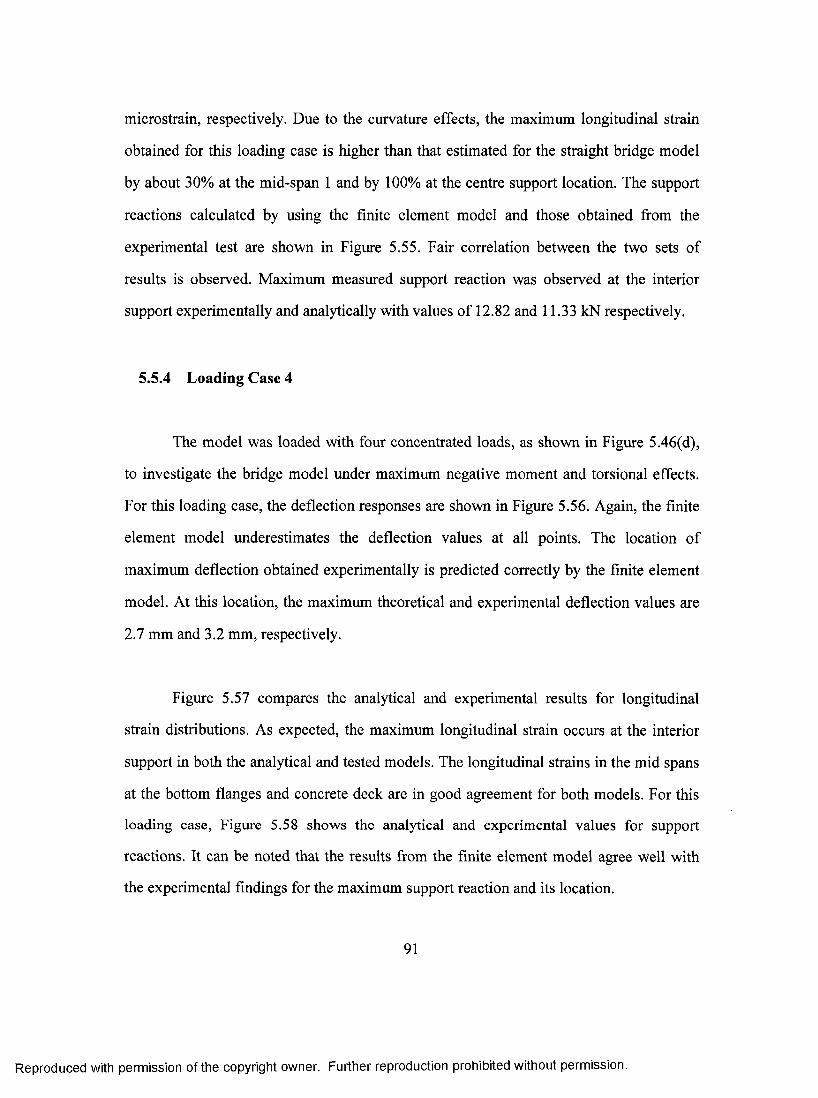
microstrain, respectively. Due to the curvature effects, the maximum longitudinal strain
obtained for this loading case is higher than that estimated for the straight bridge model
by about 30% at the mid-span 1 and by 100% at the centre support location. The support
reactions calculated by using the finite element model and those obtained from the
experimental test are shown in Figure 5.55. Fair correlation between the two sets of
results is observed. Maximum measured support reaction was observed at the interior
support experimentally and analytically with values of 12.82 and 11.33 kN respectively.
5.5.4 Loading Case 4
The model was loaded with four concentrated loads, as shown in Figure 5.46(d),
to investigate the bridge model under maximum negative moment and torsional effects.
For this loading case, the deflection responses are shown in Figure 5.56. Again, the finite
element model underestimates the deflection values at all points. The location of
maximum deflection obtained experimentally is predicted correctly by the finite element
model. At this location, the maximum theoretical and experimental deflection values are
2.7 mm and 3.2 mm, respectively.
Figure 5.57 compares the analytical and experimental results for longitudinal
strain distributions. As expected, the maximum longitudinal strain occurs at the interior
support in both the analytical and tested models. The longitudinal strains in the mid spans
at the bottom flanges and concrete deck are in good agreement for both models. For this
loading case, Figure 5.58 shows the analytical and experimental values for support
reactions. It can be noted that the results from the finite element model agree well with
the experimental findings for the maximum support reaction and its location.
91
Reproduced with permission of the copyright owner. Further reproduction prohibited without permission.
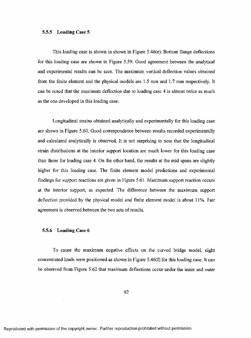
5.5.5 Loading Case 5
This loading case is shown in shown in Figure 5.46(e). Bottom flange deflections
for this loading case are shown in Figure 5.59. Good agreement between the analytical
and experimental results can be seen. The maximum vertical deflection values obtained
from the finite element and the physical models are 1.5 mm and 1.7 mm respectively. It
can be noted that the maximum deflection due to loading case 4 is almost twice as much
as the one developed in this loading case.
Longitudinal strains obtained analytically and experimentally for this loading case
are shown in Figure 5.60. Good correspondence between results recorded experimentally
and calculated analytically is observed. It is not surprising to note that the longitudinal
strain distributions at the interior support location are much lower for this loading case
than those for loading case 4. On the other hand, the results at the mid spans are slightly
higher for this loading case. The finite element model predictions and experimental
findings for support reactions are given in Figure 5.61. Maximum support reaction occurs
at the interior support, as expected. The difference between the maximum support
deflection provided by the physical model and finite element model is about 11%. Fair
agreement is observed between the two sets of results.
5.5.6 Loading Case 6
To cause the maximum negative effects on the curved bridge model, eight
concentrated loads were positioned as shown in Figure 5.46(f) for this loading case. It can
be observed from Figure 5.62 that maximum deflections occur under the inner and outer
92
Reproduced with permission of the copyright owner. Further reproduction prohibited without permission.

webs, and are well predicted by the finite element model. The maximum deflection values
are 4.0 mm and 4.7 mm as obtained from the finite element and experimental models,
respectively. It is obvious from all the previous comparisons that the finite element model
generally provides stiffer response.
Negative longitudinal moment at the interior support is evident from Figure 5.63
by observing the development of tensile strains in the concrete deck and compression
strains in the steel bottom flanges. The results from finite element model are in fair
agreement with those obtained from experimental model. Also, it is clear that there is
very little difference between the maximum longitudinal strains in both bottom flanges at
the interior support from the two models. In addition, the longitudinal strain along the
concrete deck is almost uniformly distributed. It is obvious that the concrete deck and the
presence of cross-bracings provided an excellent distribution for the strains. Comparing
these results with those obtained from the same loading case for the straight bridge shows
that the longitudinal strains at the interior support are much higher in the curved bridge
model. However, at the mid-span, the curved model shows higher values than those
estimated for the straight bridge by about 15%. Figure 5.64 shows the experimental and
theoretical results for the support reactions for this loading case. Maximum support
reaction values are 24.3 kN and 26.7 kN given by the finite element and experimental
models, respectively. Again, the finite element model appears to predict quite well the
experimental model findings in terms of support reactions. It is also interesting to note
that there is no significant change in the maximum support reaction for the straight and
curved bridge models.
93
Reproduced with permission of the copyright owner. Further reproduction prohibited without permission.
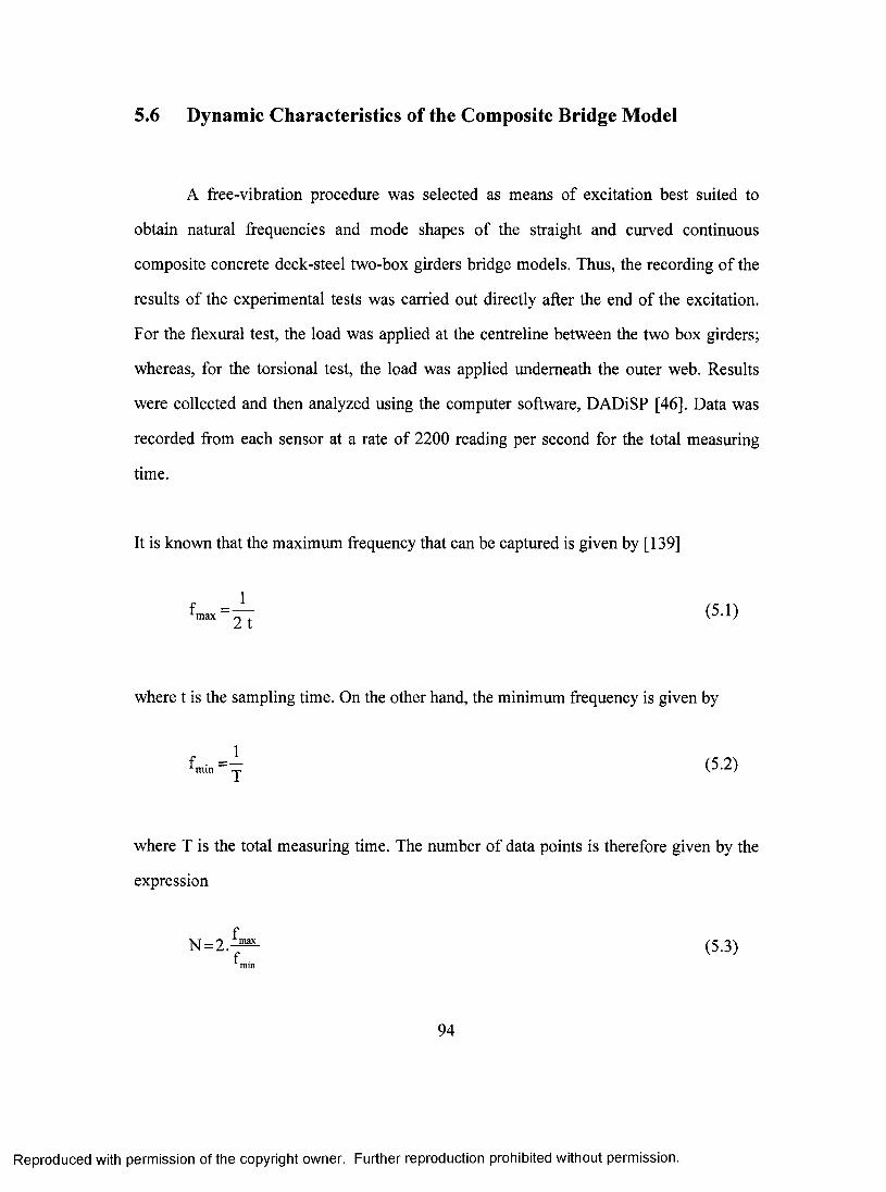
5.6 Dynamic Characteristics of the Composite Bridge Model
A free-vibration procedure was selected as means of excitation best suited to
obtain natural frequencies and mode shapes of the straight and curved continuous
composite concrete deck-steel two-box girders bridge models. Thus, the recording of the
results of the experimental tests was carried out directly after the end of the excitation.
For the flexural test, the load was applied at the centreline between the two box girders;
whereas, for the torsional test, the load was applied underneath the outer web. Results
were collected and then analyzed using the computer software, DADiSP [46]. Data was
recorded from each sensor at a rate of 2200 reading per second for the total measuring
time.
It is known that the maximum frequency that can be captured is given by [139]
(5.1)
where t is the sampling time. On the other hand, the minimum frequency is given by
4 , .= ] : (5.2)
where T is the total measuring time. The number of data points is therefore given by the
expression
N = 2 . ^ (5.3)
94
Reproduced with permission of the copyright owner. Further reproduction prohibited without permission.

Typical acceleration-time history from the accelerometers and displacement-time
history from LVDTs, obtained from the free-vibration tests on the straight bridge model
are shown in Figures 5.65 and 5.66, respectively. Similarly, for the curved bridge model,
results obtained from the accelerometers and LVDTs were recorded and typical
acceleration-time and displacement-time histories are shown in Figures 5.67 and 5.68,
respectively. Signal analysis in the frequency domain was performed on the data captured
using Fast Fourier Transform (FFT) technique. From the FFT analyzer, the spectrum
response of the bridge model in the frequency domain was calculated. Frequency spectra
for the straight bridge model from the flexural and torsional tests are shown in Figures
5.69 and 5.70, respectively. Figure 5.71 shows the frequency spectrum for the curved
bridge from the flexural test; Figure 5.72 shows for the results obtained from the torsional
test. The natural frequencies and their corresponding mode shapes were calculated, where
the peaks in frequency response suggest the locations and the values of the natural
frequencies. The values of the measured and predicted natural frequencies and their
corresponding mode shapes by the finite element model are presented in Table 5.1. It
should be noted that the measured results presented in the table are the average results
obtained from flexural and torsional tests. Table 5.2 shows the values of the fundamental
frequencies obtained experimentally for six LVDTs and six accelerometers from the
flexural and torsional tests for straight and curved bridge models. Comparing the
predictions from the fmite-element model with those obtained experimentally, good
agreement can be observed between the first two natural frequencies in both bridge
models. For the straight bridge model, the fundamental frequency values are 29.9 Hz and
31.2 Hz, obtained from the finite element model and the experimental model,
respectively, with a 4% difference. Also, the corresponding mode shape was purely
flexural in both the theoretical and experimental findings, as shown in Figures 5.73(a)
95
Reproduced with permission of the copyright owner. Further reproduction prohibited without permission.

and 5.74(a), respectively. In the case of the curved bridge model, the measured value of
the fundamental frequency was 24.5 Hz and the predicted one by the fmite-element model
was 24.1 Hz, with only 2% difference. The corresponding mode shape for the curved
bridge was a combined flexural and torsional, as given in Figure 5.73(b). This was also
confirmed by the finite element model in Figure 5.74(b). It is also interesting to note from
the these findings, that the fundamental fi-equency of the curved bridge model was lower
than the fundamental frequency of the straight bridge model by almost 29%. This
decrease in the fundamental frequency can be attributed to an increase in the degree of
curvature.
For the straight bridge model, the third and the fourth natural frequency values
were relatively close to each other, which made it difficult to extract them experimentally.
For the curved bridge model, the average third natural frequency value obtained
experimentally was 64.1 Hz. It can be observed that from Table 5.1 that the finite element
model overestimates these values by 22% for the third mode and 14% for the fourth
mode. The mode shapes of the straight and curved bridges obtained analytically and
experimentally were presented in Figures 5.73 and 5.74, respectively.
5.7 Nonlinear Response of the Composite Bridge Model
The straight and curved bridge models were loaded with two sets of concentrated
loads, symmetrically placed. Each set consisted of four equal concentrated loads. One set
was placed at 1430 mm from the interior support in each span. The load was applied at a
low rate and 10 readings per second were taken. For this loading case, the negative
moment capacity of the bridge is expected to control. The data was recorded during the
96
Reproduced with permission of the copyright owner. Further reproduction prohibited without permission.

entire loading process until failure. The loading was terminated and the models were
considered failed when they could not carry any further load, or when excessive
deflections were observed. This procedure was followed for safety reasons. Examining
the behaviour of the loaded model at its mid-span and at or near the interior support
would provide an understanding of the collapse mechanism for such bridges. Therefore,
the relationships between the applied load and deflections, steel strain and concrete strain
were investigated.
For the straight bridge model, load-deflection response is shown in Figure 5.75.
The analytical and experimental relationships between the applied load and the deflection
underneath the outer web at the mid-span are compared. It is observed that the behaviour
of the bridge model is elastic up to 250 kN. Cracks were observed on the top of the
concrete deck at about 80 kN which was observed as a kink in the load-deflection
diagram predicted by the finite element model. An increase in deflection can be observed
as the load level increases above 250 kN. However, the changes in load-deflection slope
are not pronounced due to the presence of the two layers of wire mesh in the concrete
deck. At this load level, the initial formation of the plastic hinge at the interior support
was observed. Effective plastic strain at the bottom steel flanges and extensive buckling
of the webs were also taking place. On increasing the load further, the slope of the load-
deflection curve decreased. Failure occurred by crushing of the concrete deck near the
mid-span at an approximate load of 400 kN obtained experimentally. The finite element
model estimated fairly well the load-deflection response of the tested model, predicting
an ultimate load of 365 kN.
97
Reproduced with permission of the copyright owner. Further reproduction prohibited without permission.
The results from the finite element model agreed well with the experimental
findings in predicting the longitudinal strain on the top of the concrete slab, as shown in
Figure 5.76. It is interesting to note that a significant decline in the structure stiffness is
observed at a load of 300 kN. This indicates the development of plastic strain within the
element in the maximum positive moment region. Similar observations were made for the
load-strain diagram for the bottom steel flange, as illustrated in Figure 5.77. It is obvious
that the bottom flange started yielding at a load value of about 350 kN in both the finite
and the tested models. Due to material hardening, the tested bridge model continued
carrying further load up to 400 kN when the concrete crushed, leading to failure.
Excessive deformations were also detected.
The development of the plastic hinges though the steel web at the mid span can be
followed by examining Figures 5.78 and 5.79. Analysis indicates that plastic flow started
at the bottom steel flange and propagated through the web from the bottom to the top.
The finite element model predicted the formation of the plastic hinge in the positive
moment region. This was confirmed by the results obtained from the experimental results.
For the curved bridge model, load-displacement diagram for the bottom of the
outer and inner webs are shown in Figures 5.80 and 5.81, respectively. These figures
show the deflection of the bridge model under the same loading case prescribed
previously. As can be noted from these diagrams, the behaviour of the structure model is
mainly elastic up to load of 200 kN. At this load, the concrete slab above the interior
support was extensively cracked and plastic hinges were formed. Subsequently, the bridge
model exhibited pronounced nonlinear behaviour with increasing applied load. The finite
element model corresponded well with the results obtained from the experimental model
98
Reproduced with permission of the copyright owner. Further reproduction prohibited without permission.
in terms of the deflection at the bottom of the irmermost web, but it underestimated the
deflection at the bottom of the outermost web. The finite element model estimated the
ultimate load at a value of 320 kN, on the other hand, while the maximum applied load
during the experimental test was 310 kN. The test was terminated due to large deflections
of the model near the mid-span. In addition, the tested model was not able to carry any
further load.
Load-strain relationships of the concrete deck are plotted in Figures 5.82 and 5.83,
respeetively. The finite-element model predicted fairly well the longitudinal strains at the
concrete deck. It can be observed that the finite element model showed greater structural
stiffness than that observed experimentally. Figures 5.84 and 5.85 present the comparison
between the experimental and analytical results for strains at the bottom steel flange
underneath the inner and outer webs, respectively. It can be observed that the bottom
flanges started yielding at almost 250 kN in the finite element model. It is evident from
the results that the longitudinal tensile strain under the innermost web is higher than that
under the outermost web for the same applied load, where the plastic flow near the mid
span started and spread from the bottom flange underneath the innermost web to the
bottom flange underneath outermost web.
The relationships between the applied load and the longitudinal strains for the
innermost web at mid-span are shown in Figures 5.86 and 5.87. Near the top position of
the innermost web, the finite element model results correlate quite well with the results
from the experimental model up to a load of almost 200 kN. Beyond this load, the finite-
element model overestimates the longitudinal tensile strain. Larger longitudinal tensile
strains were obtained experimentally and analytically for the bottom position of the
99
Reproduced with permission of the copyright owner. Further reproduction prohibited without permission.

innennost web, where the plastic strains near the mid-span were spreading from the
hottom flange through the weh.
Longitudinal tensile strains are plotted against the applied load for the outermost
web at mid-span in Figures 5.88 and 5.89. Again, results from the fmite-element and
tested models agreed well as long as the general structural behaviour is elastic. For a load
greater than 200 kN, the finite element model appears to be more stiff than the
experimental model. However, both models showed similar trend with respect to the
longitudinal tensile strains for the outermost web. It is also obvious that the plastic strains
started at the bottom flange and propagated through the web upward from bottom.
Figures 5.90 and 5.91 illustrate the deflected shapes of the straight and curved
tested bridge models, respectively. It should be noted that in both cases, the bridge
models exhibited large deflections prior to failure. However, for the curved bridge model,
the deflections were much more pronounced than for the straight bridge model. For the
latter, the test was terminated when excessive deformation of the bridge model was
observed. The development of cracks gives an insight into the progression of failure of
the straight and curved bridge models, as shown in Figures 5.92 and 5.93, respectively.
For the straight bridge model. Figure 5.92, the cracks are close and parallel to the interior
support line. First crack was observed on both side of the interior support at 80 kN. At
almost 200 kN, the concrete slab failed and wide cracks developed at the interior support.
This indicated that a plastic hinge had developed at the interior support.
In the curved bridge model, tracing the cracks was more complicated. The first
crack was observed at a low load of around 40 kN, and was inclined to the support line.
100
Reproduced with permission of the copyright owner. Further reproduction prohibited without permission.
Upon increasing the load, cracks progressed on the top concrete slab in the negative
moment region. At a load of 200 kN, wide cracks developed on both side of the interior
support, inclined to the support line, indicating the contribution of the torsional moment
associated with the higher curvature of the bridge model and combined with the flexural
moment. The crack pattern for the curved bridge model is shown in Figure 5.93.
Excessive deformation at the interior support at the bottom flange was observed in
both bridge models, as shown in Figures 5.94 and 5.95, respectively. Severe buckling of
the webs at the interior support was detected. It should be noted that the deformation at
the bottom flange and the buckling in the webs contributed to the development of the
plastic hinge at the interior support. Figures 5.94 and 5.95 show the deformation of the
bottom flange in straight and curved bridge models, respeetively. Cross bracing members
were investigated after terminating the test in both bridge models. No significant
deformation was detected in the straight bridge model. However, excessive deformation
in the cross bracing members was observed in the curved model due to the torsional
moments.
5.8 Discrepancies Between the Experimental and Theoretical Results
The results obtained from the experimental and finite-element models indicate
that there are some differences between the two sets. However, a reasonable agreement
within the range of the experimental and finite-element errors can be concluded. The
experimental errors lie primarily in the sensitivity of equipment measurement and the
simulation of the boundary condition. Also, the tolerance in the rolling of thin sheets used
for the webs of the bridge models may be attributed to the discrepancies between the
101
Reproduced with permission of the copyright owner. Further reproduction prohibited without permission.
experimental findings and finite element results. Finite-element errors may be introduced
as a result of structure modelling, boundary condition simulation, shear connectors
simulation, and concentrated loads. In addition, to obtain the collapse load, the explicit
method was adopted to analyze the finite-element model, where the model was subjected
to vertical displacement at the load location points. Material modelling can contribute to
the fmite-element errors, particularly in the study of the nonlinear response of the bridge
models. In the case of the reinforced concrete deck, effects associated with the
rebar/concrete interface, such as bond slip and dowel action, are modeled approximately
by introducing tension stiffening into the concrete modelling to simulate load transfer
across cracks through the rebar. Also, welding between steel plates can be regarded as
constrained points.
5.9 Summary
The structural elastic responses of non-composite and composite continuous two-
box bridge models were examined analytically and experimentally. The inelastic
behaviour as well as the dynamic characteristic was determined for the two composite
bridge models. The finite element commercial program ABAQUS/standard was utilized
to obtain the elastic behaviour and free-vibration analysis. The finite element
ABAQUS/explicit was employed to investigate the structural nonlinear response of such
bridges.
Comparisons between the two sets of results were carried out in terms of vertical
deflection, longitudinal strain, support reaction, natural frequency, mode shape as well as
the collapse load. The comparisons indicate both the reliability of ABAQUS ‘s model in
102
Reproduced with permission of the copyright owner. Further reproduction prohibited without permission.
predicting the actual structural responses elastically and inelastically. The physical and
analytical models were in fair to good agreement for all load cases with a reasonably
small percentage of errors. These errors could be attributed to both experimental and
modelling reasons. The experimental errors include: measurements, loading and
unloading, boundary conditions and equipment calibration. Errors in the finite element
modelling can be attributed to: load application, interaction between the concrete and the
steel, boundary conditions and material properties.
Generally the structural stiffness of the fmite-element model is higher than that of
the physical model. As a result, in the elastic loading cases, the finite element model has
underestimated the deflection and overestimated the reactions of the bridge model. It is
also interesting to note that the finite element model estimated the fimdamental frequency
of the bridge models within 5% of the experimental findings. Also, the corresponding
mode shape was accurately predicted. The inelastic responses of the analytical models
were in good correlation with the experimental readings. This validates the use of the
finite element model in predicting the elastic and inelastic behaviour of such bridges. The
finite element model underestimated the collapse load in the case of straight bridge model
by 10% from the experimental results, and overestimated it by 5% for the curved bridge
model.
The reasonable correlation between analytical and experimental findings
presented in this chapter for all loading cases in the static and dynamic tests point to the
following:
103
Reproduced with permission of the copyright owner. Further reproduction prohibited without permission.

1. The finite element analysis can reliably predict the static and dynamic
responses as well as the inelastic behaviour of continuous composite box
girder bridges.
2. Loading the outer lane in a continuous curved box girder bridge produces
the maximum vertical deflection, longitudinal strains as well as support
reaction.
3. The vertical deflection, longitudinal strain and support reactions obtained
for a curved bridge are much higher than those for the straight bridge
model.
4. The presence of the concrete deck and the cross bracing inside and
between the boxes enhances the overall structural performance of such
bridges. They are effective in distributing the flexural and torsional
moments throughout the bridge cross-section.
5. The fundamental frequency of such bridges decreases significantly with
increase in bridge curvature.
6. Inelastic structural behaviour as well as the ultimate load of continuous
composite box girder bridges can be well predicted by the finite element
model.
104
Reproduced with permission of the copyright owner. Further reproduction prohibited without permission.
CHAPTER VI
Parametric Studies
6.1 Introduction
Parametric studies were performed on continuous curved two-equal-span bridges
having a eoncrete deck on multiple steel box girders. The objectives of the studies were
to: (1) examine the influence of key parameters affecting the structural response; (2)
establish a data base for the various distribution factors, for maximum stresses,
deflection, shear force, and support reaction forces necessary for design; (3) generate
information as yet unavailable for the impact factors for maximum stresses, deflection,
shear force, and support reaction forces; (4) investigate the dynamic behaviour of sueh
bridges; and (5) deduce empirical formulas for load distribution factors, impact factors,
and fundamental frequencies.
The results for the load distribution factors were obtained for traffic live loading
and self-weight of the bridges. AASHTO live loading was mainly used in the parametric
study for the load distribution factors. Subsequently, these load distribution factors were
examined for various truck loading types by applying AASHTO LRFD, CHBDC, and
CHBDC-ONT live loadings. However, only AASHTO truck loading was considered in
the generation of the impact factors. A parametric study was also conducted using free
vibration analysis to obtain the fundamental frequencies of such bridges.
105
Reproduced with permission of the copyright owner. Further reproduction prohibited without permission.
6.2 Description of Bridges Used in the Parametric Studies
In the parametric study for load distribution factors, the effects of the following
main parameters that influence the load distribution in the studied bridges: (1) number of
lanes, Nl; (2) number of boxes, Nb; (3) span length, L; (4) span-to-radius of curvature
ratio, K = L/R. The choice of these parameters was based on other studies [9, 63]. The
same variables were also applied in the parametric studies for impact factors and
fundamental frequencies.
Table 6.1 presents the sectional configurations examined for the bridges used in
the parametric study for the load distribution factors, while. Table 6.2 shows the bridges
considered in the parametric studies for impact factors and fundamental frequencies. The
symbols used in Tables 6.1 and 6.2 represent designations of the bridge types considered
in these parametric studies: / stands for lane; b stands for box; and the number in the
middle of the designation embodies the span length of the bridge in meters. For example,
4/-80-6Z> denotes a continuous two-equal-span bridge of four lanes, 6 boxes and each span
being 80 m long. The cross-sectional symbols used in Tables 6.1 and 6.2 are showm in
Figure 6.1.
Five different lengths of 20, 40, 60, 80, and 100 m for each span were considered
in all the parametric studies. Such a range of spans covers medium span bridges. The
number of lanes was taken as 2, 3, and 4 lanes. According to Geometric Design Standards
for Ontario Highways [96], the lane width for two or more lanes should be 3.75 m.
Providing two sidewalks, one on each side of the bridge, of 0.9 m for all bridges, the total
bridge width would be 9.30 m in the case of two-lane, 13.05 m in the case of three-lane
106
Reproduced with permission of the copyright owner. Further reproduction prohibited without permission.
and 16.80 m in the case of four-lane bridges. The number of boxes ranged from two to
four in the case of two-lane bridges, two to six in the case of three-lane bridges, and three
to six in the case of four-lane bridges. Figure 6.2 presents the number of boxes along with
the number of lanes considered in the parametric studies.
The curved bridges considered in the parametric studies were assumed to have
constant radii of curvature for both spans. The degree of curvature defined as span-to-
radius of curvature ratio, k = L/R, where the span length of the each bridge span, L, is the
arc length along the centreline of its cross-section and the radius of curvature, R, is the
distance from the origin of the circular arc to the centreline of the cross-section. The L/R
ratios used in the parametric study for the load distribution factors were 0.0, 0.1, 0.2, and
0.4 in the case of span lengths of 20 and 40 m, and 0.0, 0.4, 0.8, and 1.2 in the case of
span lengths of 60, 80, and 100 m. However, in the parametric studies for the impact
factors and fundamental frequencies, the L/R ratios were taken as 0.0, 0.1, 0.2, and 0.4 in
the case of span lengths of 20 and 40 m, and 0.0, 0.4, 0.6, and 1.2 in the case of span
lengths of 60, 80, and 100 m. The values of the radius of curvature were selected to be in
accordance with the Geometric Design Standard for Ontario Highways [96], which
requires that the radius of curvature be no smaller than 45 m.
The practical range of span-to-depth ratio for box girder bridges range from 20 to
30 [62]. For steel girders having a specified minimum yielding stress of 350 MPa or less,
the preferred span-to-depth ratio of the steel girder is not to exceed 25 [62], where the
span to be used in determining this ratio is defined as 0.9 times the arc length for
continuous end spans. In a curved bridge, each box girder in the bridge cross-section is
likely to deflect differently. Increasing the depth, and hence the stiffness, of the girders in
107
Reproduced with permission of the copyright owner. Further reproduction prohibited without permission.
curved bridge leads to smaller relative differences in the deflections and smaller cross
bracing forces. Therefore, the span-to-depth ratio was slightly relaxed to 25.
Interior diaphragms were provided inside the box girders at each support in the
radial direetion. The end diaphragm thicknesses were taken to be the same as those of the
webs in all cases. The depth of the diaphragms was taken the same as the depth of the
steel box. A sensitivity study had shown that the aecess holes through the diaphragms had
an insignificant effect on the overall structural response of the bridges. Therefore, solid
end diaphragms were assumed inside the boxes at all supports and bracings were
provided between the boxes at support lines, as shown in Figure 6.1, to resist torsion and
deformation. Intermediate eross braeings were also placed at a spacing of 5 m for all
bridge configurations. Based on a study by Sennah [124] on curved simply supported
bridges, it was shown that this spacing is quite adequate in case of eellular bridges.
Moreover, this spacing is less than the maximum of 7.5 m recommended by AASHTO
Standard [3]. Permanent intermediate external eross braeings between boxes are usually
unnecessary. However, temporary intermediate external bracing may be desirable to
prevent or alleviate the twisting of boxes during casting of the concrete deck slab. In
addition to the cost, the removal of the intermediate external bracing may increase the
stresses in the concrete deek slab. Therefore, in this parametric, intermediate external
bracings were provided at the same spacing as the internal bracings.
Top chords internal to the tub steel girders were placed at the support lines to help
control twist and distortion. A sensitivity study conducted by Sennah [124] revealed that
replacing the area of angle cross-section by a rectangular cross-section for the top chord
showed no effect on the structural response of the bridges. Moreover, changing the
108
Reproduced with permission of the copyright owner. Further reproduction prohibited without permission.
stiffness of the rectangular bracing systems or replacing the bracing system by an
equivalent solid plate member of the same volume has also shown no significant effect on
the elastic structural behaviour, irrespective of the degree of curvature. Accordingly, all
X-type bracing members and top chords were chosen to be of 100 x 100 mm rectangular
cross section in all bridges.
The effect of the thickness of the bottom flange and web on the distribution
factors was investigated for 4/-60-36 bridge having L/R = 0.4, where the local buckling of
the steel plates and the plastic behaviour of the materials were not considered in this
study. Figures 6.3 and 6.4 show the influence of the thickness of bottom flange and web,
respectively, on the distribution factor for tensile stress on the AASHTO truck load and
dead load. It should be noted that the change in the thickness of the bottom flange or web
has less than 3% effect, in the case of the live load, and less than 1%, in the case of dead
load. A study conducted by Zhang et al. [150] showed that the bottom flange or web
thickness has no significant effect on the impact factors for horizontally curved composite
bridges. Therefore, the thickness of the bottom flange and web were taken constant
through the parametric studies.
A preliminary sensitivity study regarding the change in flexural stiffness of the
bridge revealed that changing the span-to-depth ratio of the steel section has more effect
on the structural response than changing the concrete slab thickness. Therefore, the
thickness of the concrete deck was kept constant for all bridges considered in the
parametric studies. For all bridges used in the parametric studies, the moduli of elasticity
of concrete and steel were taken as 27 and 200 GPa, respectively. Possion’s ratio was
taken as 0.2 for concrete and 0.3 for steel.
109
Reproduced with permission of the copyright owner. Further reproduction prohibited without permission.

6.3 Loading Conditions
The bridges were analyzed under the effect of their self-weight and highway
traffic loadings. The behaviour of curved box girder bridges is unsymmetrical by nature.
As a result, it docs not seem reasonable to distribute the dead loads equally to all box
girders in sueh bridges. Consequently, the assumption made by North American Codes of
Practice [3, 4, 5, 6, 7, 20] that the dead load is considered distributed uniformly between
box girders does not seem to be accurate for curved bridges. Moreover, the traffic loads is
even more unevenly transferred to the box girders. AASHTO live loading was adopted in
the parametric studies to investigate the distribution of live loads. The load distribution
factors were also compared with those obtained by considering AASHTO LRFD,
CHBDC and CHBDC-ONT live loadings. For the study of impact factors, only AASHTO
truck loading, HS20-44, was used in the dynamic analysis.
6.3.1 Dead Load
The dead load due to self-weight of the bridges was considered. Gravity was
specified by the constant, g = 9.81 m/s^. In addition, the material densities were taken as
2400 kg/m^ for concrete and 7800 kg/m^ for steel. Thus, the self-weight of the bridge can
be calculated from these values.
6.3.2 Live Load
AASHTO Standard truck load HS20-44 as well as the equivalent lane load was
considered in the parametric study for the load distribution factors. The truck loading,
110
Reproduced with permission of the copyright owner. Further reproduction prohibited without permission.
HS20-44, with a total load of 325 kN is shown in Figure 6.5. The equivalent lane load
consisted of superimposed load of 9.3 kN/m uniformly and centrally distributed within
strip of 3.0 m plus a single concentrated load distributed over 3.0 m width on a line
normal to the centreline of the lane. The single concentrated load was taken as 80 kN to
generate the stress distribution factors and 116 kN to generate the shear distribution
factors. Modification factors of 1, 0.9, and 0.75 for two-, three-, four-lane loading,
respectively, were applied to account for multiple lanes loading in accordance with
AASHTO standard [3].
To obtain the load distribution factors, the above two types of loading were first
applied to a two-equal-span continuous straight girder with a span equal to the span
length of the centreline of one of the two spans of the bridge, to determine which load
type will cause maximum effects. As a result of this investigation, it was established that
the truck loading HS20-44 would be used in the case of bridges with 20 and 40 m span
lengths, and the equivalent lane loading plus the eoncentrated load would be applied for
bridges with 60, 80, and 100 m span lengths.
In order to determine maximum response, two loading cases were applied to each
bridge in the transverse direction using the finite element analysis, viz., full and partial
AASHTO truck loading (or equivalent lane loading) as shown in Figure 6.6. In the partial
loading case, the wheel loads close to the curbs were positioned at a distance of 0.6 m
from the eurb edge of the bridge and the outer lane was loaded to produce the maximum
torsional effects. However, in the parametric study of impact factors, only full AASHTO
truck loading was analyzed in the dynamic analysis for all bridges considered herein, as
shown in Figure 6.7.
I l l
Reproduced with permission of the copyright owner. Further reproduction prohibited without permission.

In the AASHTO LRFD [7], the effect of the truck loading or design tandem is
combined with the lane load in the design. Both the design lane load and the truck
loading are the same as those used in the AAHSTO standard. The design tandem consists
of a pair of 110 kN axles spaced 1.2 m apart. Modification factors based on AASHTO
LRFD are 1, 0.85, and 0.65 for two-, three-, four-lane loadings, respectively. A different
vehicular loading is specified in the case of CHBDC of 2000 [20]. The CL-625 truck
loading as well as the lane loading is considered in the design of bridges everywhere in
Canada except in Ontario, where CL-625-ONT truck is applied instead of CL-625 truck.
The lane loading consisted of superimposed load of 9 kN/m uniformly and centrally
distributed within a strip of 3 m width. The truck loading, or 80% of the truck loading
combined with the lane load, whichever produces higher structural responses is applied.
The modification factors applied in accordance with CHBDC of 2000 [20], are: 0.9, 0.8,
and 0.7 for two-, three-, four-lane loading, respectively.
6.4 Parametric Study for Load Distribution Factors
To calculate the load distribution factors for the bridges, an extensive parametric
study was carried out. The parametric study was conducted on two-equal-span continuous
curved concrete deck on multiple steel box girder bridges to achieve all the objectives
stated in section 6.1. The key parameters chosen for this parametric study were also stated
earlier. In addition, the influence of the inclined webs, span-to-depth ratio, and the cross
bracings on the load distribution factors were examined.
The assumptions made in the parametric study were as follows: (1) the reinforced
concrete slab deck had complete composite action with the top flange of the box girders
112
Reproduced with permission of the copyright owner. Further reproduction prohibited without permission.

through the presence of the shear connectors; (2) the analysis was conducted assuming
the behaviours of the steel and concrete were elastic and homogenous. Thus the effect of
the plastic deformation or local buckling has not been considered in the analysis; (3) the
effects of the road superelevation, outer-web-slopes, curbs and railings were not taken
into account; (4) solid diaphragms at the support lines were used in the radial directions;
(5) the bridges had constant radii of curvature between support lines; (6) to avoid stresses
due to the effect of supports constrained in plan, bearing A at the inner support line (pier).
Figure 3.8, was constrained in two directions and the innermost bearings on the outer
support lines (abutments) were constrained in the direction perpendicular to the line from
A to that bearings B at the outer support lines (abutments) [118]; all other bearings at the
abutments remained free to move along the horizontal plan of the bridge; and (7) the
truck wheel loads were simulated as concentrated loads.
The load distribution factors for the bridge straining action were calculated by
dividing the maximum straining action determined from the finite element analysis of
three-dimensional bridge by the maximum value for the corresponding straining action
for an idealized girder. The idealized girder was formulated by partitioning the two-span
continuous composite multiple box girder cross section of the bridge to a number of
individual girders, as shown in Figure 6.8. The span lengths for the idealized girder are
exactly the corresponding centreline lengths of the bridges. Each individual girder
consisted of one steel web, steel top flange, ( A / 2 N b ) portion of concrete deck slab, and
( A / 4 N b ) wide steel bottom flange, where A = bridge width and N b = number of boxes.
A form of the function to be fitted to the data collected from the finite element
analysis was specified using several trials. A nonlinear regression analysis was performed
113
Reproduced with permission of the copyright owner. Further reproduction prohibited without permission.

to determine the values of parameters for a function that cause the function to best fit the
set of data obtained from the finite element analysis. The goal of this technique is to
evaluate the values of the parameters that minimize the sum of the squared residuals
values for the set of observations. That is known as a Least Square regression fit. The
sum of the squared differences between the actual value of the dependent variables for
each data and the value predicted by the function, using the final parameters, was
calculated. The average deviation over all observations of the absolute value of the
difference between the actual value of the dependent variable and its predicted value was
calculated.
6.4.1 AASHTO Live Loading
Several loading cases were considered in the transverse and longitudinal
directions for each bridge to obtain the maximum straining actions. In the longitudinal
direction, the truck loadings, or the equivalent lane loading plus the corresponding
concentrated load, were placed as follows: (1) AASHTO live loading near the mid-span
to produce the maximum tensile stresses and deflection at the bottom flange, as presented
in Figure 6.9(a); (2) AASHTO live loading in both spans as shown in Figure 6.9(b) to
evaluate the maximum compression stresses in the bottom flange at the interior support;
(3) AASHTO live loading in one span at 1 m distance from the outer support line, as
shown in Figure 6.9(c) to obtain the maximum shear force and the reaction force at the
exterior support; (4) AASHTO live load on both spans to get the maximum shear force at
the interior support, as shown in Figure 6.9(d); and (5) AASHTO live load in each span to
get the maximum reaction at the interior support, as illustrated in Figure 6.9(e).
114
Reproduced with permission of the copyright owner. Further reproduction prohibited without permission.
All AASHTO live loading cases were applied twice, fully and partially loaded
lanes. Using the finite element analysis for the three-dimensional bridge, maximum
straining actions were obtained for all the loading cases and then multiplied by the
corresponding modification factors. The minimum reaction force (uplift) was estimated
by considering the minimum reaction at all support points in all loading cases. Figure 6.6
shows the location of live load in the transverse direction of the bridges.
The maximum tensile stress, Op, was obtained in the three-dimensional bridge
using the finite element analysis. The two-equal-span continuous idealized girder was
loaded with the total AASHTO live loading on the bridge divided by the number of
idealized girders to produce the maximum positive moment near the mid-span. Then, the
maximum tensile stress at the bottom fibre near the mid-span, Opa, for the idealized girder
was calculated using the simple beam bending formula. Thus, the distribution factor for
tensile stress, Dnp, in the bridges was calculated from the following formula:
= — (6 .1)
The distribution factor for compressive stress was formulated in the same manner
as that for the distribution factor for tensile stress. From the finite element analysis of the
bridge, the maximum compressive stress, a„, was calculated. Again, the two-equal-span
continuous idealized girder was loaded with the total AASHTO live loading on the bridge
divided by the number of idealized girders to produce the maximum negative moment at
the interior support. The maximum compression stress at the bottom fibre at the interior
support, Ona, for the idealized girder was calculated using the simple beam bending
115
Reproduced with permission of the copyright owner. Further reproduction prohibited without permission.

formula. The distribution factor for compressive stress, Den, in the bridges was
determined from:
D a n = — ( 6 . 2 )
According to the North American Codes of Practice for bridges [3, 20], the
limiting value of the live-load deflection is specified in the form of the span length, span-
to-depth ratio, or first flexural frequency. The maximum live-load deflection of each
girder of the bridge cross section is preferably limited to L/800, except for the girders
under the sidewalks for which the live-load deflection is preferably limited to L/1000
[62], where L is taken as the girder arc length between the support lines. Therefore, the
deflection due the live load should be considered in the design of bridges. The deflection
distribution factor was developed by obtaining the maximum deflection under the webs,
6, and the maximum deflection of the idealized girder, 5a. Thus, the deflection
distribution factor, Dg, was calculated as:
D6 = | - (6.3)
In order to determine the shear distribution factor, Dy, the maximum shear forces
in the three-dimensional bridge, V, and the maximum shear force in the corresponding
idealized girder, Va, were first calculated. It must be noted that the maximum shear forces
of the bridges were obtained by considering the absolute maximum values, regardless of
the loading case or the location of the shear force in the box girders. The shear
distribution factor was then calculated from the following relationship:
116
Reproduced with permission of the copyright owner. Further reproduction prohibited without permission.

D. = ^ (6.4)V.
Distribution factors for the exterior reaction forces, Dg, were also determined in
the similar way as those for the shear distribution factors. The maximum exterior reaction
considering all loading cases, Rg, was estimated from the three-dimensional finite element
analysis of bridges. Then, the maximum reaction force at the exterior support, Rea, was
calculated for the idealized girder. The exterior reaction distribution factor was calculated
from;
D e = - ^ (6.5)^ea
In the same fashion, the distribution factor for the interior reaction force, Dj, was
formulated as:
(6.6)^ia
where Rj is the maximum reaction force at the interior support obtained from all the
loading cases considered in the parametric study, and Rja is the maximum reaction force
at the interior support of the corresponding idealized girder.
The minimum reaction force, Rm, was determined at all support lines from all
loading cases considered in the parametric study for each bridge. To obtain the uplift
(minimum reaction) distribution factors. Dm, the minimum reaction force calculated from
117
Reproduced with permission of the copyright owner. Further reproduction prohibited without permission.
the finite element analysis of the bridge was divided by the maximum reaction force at
the exterior support for the idealized girder, Rea, thus,
= - ^ (6.7)^ea
6.4.2 Dead Load
To obtain load distribution factors for dead load, the maximum tensile and
compressive stresses in the steel bottom flange, Opa and ana, respectively, the maximum
deflection, 6a, the maximum shear force, Va, the maximum exterior and interior reactions,
Rea and Rja, respectively, were first calculated for a two-equal-span continuous idealized
girder, loaded by a uniform load q, where q = total dead load/ 2 Nb, where Nb is the
number of boxes. The moment of inertia used in calculating the maximum tensile and
compressive stresses corresponded to that of the composite section which included both
the steel girders and portion of the concrete deck slab. Thus, to determine the distribution
factors for the tensile, compressive stresses, gcp, g^n, deflection, gs, shear force, gv,
exterior reaction, ge, interior reaction, gj, and minimum reaction, gm, due to the dead load
the maximum tensile and compressive stresses, ap and a„, deflection, 6, shear force V,
exterior reaction. Re, interior reaction force, Ri, and the minimum reaction force, R^,
were calculated from the finite element analysis for each of the bridges subjected only to
its self-weight. Thus, the distribution factors for dead load were formulated as follows:
9 a p = — (6.8)
118
Reproduced with permission of the copyright owner. Further reproduction prohibited without permission.
Qan = (6.9)
98 = (6.10)
9v = V(6 . 11)
Req = —^ (6 .12)
9i = - ^3 iiR„
(6.13)
9 m =R„ (6.14)
where the symbols are explained under “Notations”
6.5 Parametric Study for Impact Factors
A sensitivity study was first undertaken to determine the influence of different
parameters such as the vehicle speed on the impact factors. Table 6,3 presents the vehicle
speed considered in the parametric study for impact factors for all bridges. This will be
discussed further in Chapter VIII.
119
Reproduced with permission of the copyright owner. Further reproduction prohibited without permission.

In this parametric study, full loaded lanes with AASHTO trucks HS20-44 were
considered. Each truck travelled with a constant speed along the centreline arc of the
loaded lane. The travelling speed was considered in accordance with the maximum safe
allowable highway speed. It must be stated that in the longitudinal direction of each
bridge, two trucks were placed at certain distance to produce the maximum compressive
stresses at the bottom flange at the interior support line. Static and dynamic analyses were
conducted for each bridge subjected exactly to the same loading condition. The maximum
tensile and compressive stresses, deflection, shear force, exterior and interior reactions,
and the minimum reaction were estimated from both static and dynamic analyses. Thus,
the impact factor for each straining action was obtained by dividing the increase in the
straining action due to the dynamic effect by the straining action resulting from the static
analysis.
6.6 Parametric Study for the Fundamental Frequency
This parametric study was undertaken using free vibration analysis to investigate
main parameters that may influence the natural frequencies and mode shapes of
continuous curved concrete deck-on multiple steel box girder bridges. The mode shapes
of two-equal-span curved bridges are generally either symmetric or antisymmetric about
the interior support line. Schematic views of these mode shapes are shown in Figures 6.10
and 6.11. As a result of an extensive parametric study of 180 bridges, empirical
expressions to estimate the fundamental frequency for each bridge were deduced, together
with recommendations for increasing the torsional resistance of continuous curved
bridges.
120
Reproduced with permission of the copyright owner. Further reproduction prohibited without permission.

CHAPTER VII
Load Distribution Factors
7.1 Introduction
Despite all the inherent advantages of a curved composite concrete deek-steel
multiple box girder bridge, its behaviour is more complex than that of the I-girder bridge.
Bridge designers in North America strongly prefer a simplified method of analysis to
reduce the complexity involved in the load distribution analysis of a bridge. Accordingly,
in this chapter the results from a rigorous parametric study are presented. Three-
dimensional finite-clement models are used in the analysis, in which 240 two-span
composite multiple box-girder bridges are studied. Various loading conditions are
considered to evaluate the results for the maximum structural responses of such bridges.
The results from the parametric study are based on AASHTO live load and the
bridge self-weight. The following are obtained: (i) the distribution factor for tensile
stress; (ii) the distribution factor for compressive stress; (iii) the distribution factor for
deflection; (ix) the distribution factor for shear force; (x) the distribution factor for
maximum exterior reaction force; (xi) the distribution factor for maximum interior
reaction force; and (xii) the distribution factor for minimum reaction force (uplift). The
effects of bridge span length, number of lanes, number of boxes and span-to-radius of
curvature on the structural responses of the bridges are discussed. Moreover, the effects
of the number of bracing members on the distribution factors are investigated. Empirical
121
Reproduced with permission of the copyright owner. Further reproduction prohibited without permission.
expressions for these distribution factors corresponding to the AASHTO live load and
dead load are deduced. Furthermore, the effects of the number of bridge spans on the
distribution factors are examined as well as the influence of inclined webs in the steel box
girder. Sensitivity study on three bridges is conducted to evaluate the effect on the
aforementioned distribution factors due to AASHTO LRFD, CL-625, and CL-625-ONT
truck loadings.
7.2 Distribution Factors for Tensile Stress
7.2.1 Effect of Span Length
Figures 7.1(a) and 7.1(b) show the distribution factors for maximum longitudinal
tensile stress in four-lane three-box girder bridges with L/R = 0.0 and 0.4 due to
AASHTO live load and dead load, respectively. For both loading cases, it can be
observed that the stress distribution factors for straight bridges decrease by about 12%
with increasing span length from 20 m to 60 m. For straight bridge with span length
exceeding 60 m, the distribution factor for tensile stress changes by less than 1%. In the
case of curved bridge, the distribution factors for tensile stress are affected by the span
length, with differences not exceeding 14 %.
7.2.2 Effect of Number of Lanes
The bridge width, represented by the number of lanes, is considered to be one of
the criteria that affect the distribution factor for tensile stress in curved bridges. The
distribution factors for longitudinal tensile stress in curved bridges with four boxes and
122
Reproduced with permission of the copyright owner. Further reproduction prohibited without permission.

span lengths of 20 m and 60 m, due to AASHTO live load and dead load are shown in
Figures 7.2(a) and 7.2(b), respectively. It can be observed that the distribution factors
vary almost linearly with the number of lanes varies for both span lengths. The
distribution factor for tensile stress decreases with increasing number of lanes for
AASHTO live load. However, for bridges with span length of 60 m, the changes in the
distribution factor for tensile stress are higher than those obtained for bridges with span
lengths of 20 m. The distribution factor for tensile stress under the self weight of the
bridge increases by almost 10% for short span bridges and becomes almost constant for
bridges with longer span lengths.
7.2.3 Effect of Number of Boxes
The effects of the number of box girders on the distribution factor for tensile
stress for two bridges having different span lengths are illustrated in Figures 7.3(a) and
7.3(b) for AASHTO live load and dead load, respectively. The distribution factor for
tensile stress is almost uniform in case of live load irrespective of the number of boxes
for bridges with span length of 40 m. However, it increases by about 13% with increase in
the number of boxes from 2 to 6 for bridges with span lengths of 100 m. In the case of
dead load. Figure 7.3(b) shows a small increase in the distribution factor for tensile stress
when more boxes are added. The above results reveal that increasing the number of boxes
may not result in a cost effective design in most cases in terms of tensile stresses.
123
Reproduced with permission of the copyright owner. Further reproduction prohibited without permission.
7.2.4 Effect of Span-to-Radius of Curvature Ratio
As expected, the span-to-radius of curvature ratio of box girder bridges had a
significant effect on the distribution factor for tensile stress. Figure 7.4(a) shows the
relationship between the distribution factor for tensile stress and the span-to-radius of
curvature ratio for AASHTO live load. It can be noted that for both bridge span lengths,
considered herein, the distribution factor for tensile stress increases significantly with
increase in the span-to-radius of curvature ratio. Similar trends are observed in Figure
7.4(b) for the distribution factors due to the bridge self weight. Interestingly these two
figures show that the longitudinal tensile stress increases by almost 40% for the same
bridge configurations when the L/R is increased from 0 to 1.2.
7.3 Distribution Factors for Compressive Stress
7.3.1 Effect of Span Length
The results for the bridge span length effect on the distribution factors for
compressive stress are presented in Figures 7.5(a) and 7.5(b), for AASHTO live load and
the bridge dead load, respectively. It is observed that the distribution factors for
longitudinal compressive stress decrease when the bridge span length changes from 20 m
to 40 m. Increasing the span length beyond 40 m, increases somewhat the distribution
factors for compressive stress. This observation was noted for bridges under AASHTO
live load for both straight and curved bridges. This may be attributed to the fact that
maximum compressive stress obtained in the case of 20 m and 40 m bridges are based on
AASHTO live load case. For bridges with larger span length, maximum values are
124
Reproduced with permission of the copyright owner. Further reproduction prohibited without permission.

obtained from AASHTO lane loading. In the case of bridge self-weight, the distribution
factors for compressive stress increase generally by almost 6% with increasing span
length for both straight and curved bridges from 40 to 100 m.
7.3.2 Effect of Number of Lanes
The relationship between the distribution factors for compressive stress versus
number of lanes in bridges due to AASHTO live load and bridge dead load are plotted in
Figures 7.6(a) and 7.6(b), respectively. It can be observed that the distribution factors for
compressive stress vary almost linearly with the number of lanes in both figures. It is
interesting to note that the distribution factors for compressive stress increase by almost
3% with the number of lanes only for bridges under their own weight. In contrast, these
factors decrease by almost 11% with increasing number of lanes for bridges subjected to
AASHTO live load. The rate of variation in the factors for live load is greater than that in
the case of self-weight.
7.3.3 Effect of Number of Boxes
Distribution factors for compressive stress of three-lane box-girder bridges with
span-to radius of eurvature ratio of 0.4 are plotted against the number of box-girder as
shown in Figures 7.7(a) and 7.7(b), for AASHTO live load and self-weight, respectively.
It can be observed that the live load distribution factors increase by about 10% with
increase in the number of box girders. It is also interesting to observe that the minimum
value of distribution factors can be obtained when the number of boxes is almost the
125
Reproduced with permission of the copyright owner. Further reproduction prohibited without permission.
same as the number of lanes. The same observation can be made for self-weight, Figure
7.7(b).
7.3.4 Effect of Span-to-Radius of Curvature Ratio
Figures 7.8(a) and 7.8(b) present the influence of the span-to-radius of curvature
ratio on the distribution factors for compressive stress for AASHTO live load and the
bridge self-weight, respectively. The results show that the higher this ratio is, the higher
the distribution factors for compressive stress are under either live or dead loads. It should
be noted that the distribution factors of 100-m span length bridge with L/R value of 1.2
are higher by more than 65% than those obtained for straight bridges with the same span
lengths. Moreover, in some cases the maximum compressive stress is developed when
only one span is loaded, particularly for bridges with larger span length and span-to-
radius of curvature ratio. In this specific case, high longitudinal compressive stresses
occur at the interior support line due to the combined bending and torsional moments.
Occasionally with only one span loaded, unbalanced forces on the two sides of the
interior support line cause larger stresses than those determined by loading
simultaneously the two spans of the bridge.
7.4 Distribution Factors for Deflection
7.4.1 Effect of Span Length
Distribution factors for maximum deflection versus the span length for four-lane
three-box girder bridges are plotted in Figures 7.9(a) and 7.9(b) for AASHTO live load
126
Reproduced with permission of the copyright owner. Further reproduction prohibited without permission.

and self-weight, respectively. Clearly, the distribution factors for maximum deflection
occur for bridges with span length of 20 m, decreasing by about 45% as the span length
increases from 20 to 100 m. However, the rate of the decrease in the distribution factors
for deflection levels off with increase in the span length from 40 m to 100 m for bridges.
7.4.2 Effect of Number of Lanes
Similar to the variations in the distribution factors for tensile and compressive
stresses with numbers of lanes, the number of lanes also influences the distribution
factors for deflection in the same marmer. For AASHTO live load. Figure 7.10(a) shows
the reduction in the distribution factors for deflection by about 11% with increase in the
number of lanes from 2 to 4. Figure 7.10(b) shows an increase by almost 11% in the
factors with numbers of lanes for self-weight.
7.4.3 Effect of Number of Boxes
The relationships between the distribution factors for deflection and the number of
boxes are illustrated in figure 7.11(a) and 7.11(b) for bridges subjected to AASHTO live
load and dead load, respectively. The results in both graphs exhibit the same pattern.
Increasing the number of boxes produces a change of about 5% in the distribution factors
for deflection in all cases, irrespective of the span length. The distribution factors for
deflection remain almost unchanged as the number of boxes is increased from 3 to 6 for
bridges subjected to their dead load or to AASHTO live load.
127
Reproduced with permission of the copyright owner. Further reproduction prohibited without permission.

7.4.4 Effect of Span-to-Radius of Curvature Ratio
Figures 7.12(a) and 7.12(b) show the relationship between the distribution factors
for deflection with the span-to-radius of curvature ratios for bridges subjected to
AASHTO live load and self-weight, respectively. The distribution factors for deflection
increase by almost 46% as the span-to-radius of curvature ratio increases from 0 to 1.2.
Furthermore, the trend of the increase is the same irrespective of the span length.
7.5 Distribution Factors for Shear
7.5.1 Effect of Span Length
Distribution factors for maximum shear force are plotted for 4/-3Z> straight and
curved bridges in Figures 7.13(a) and 7.13(b) for AASHTO live load and dead load,
respectively. Under AASHTO live load, distribution factors for shear are almost the same
for spans between 20 m and 40 m for straight and or curved bridges. For spans greater
than 40 m, the distribution factors for straight bridges approach unity. This means that the
live load will be distributed evenly on all bridge girders. In contrast, the distribution
factors for curved bridges increase by 8% due to an increase in the torsional effects
present in the curved bridges with larger span lengths. On the other hand, distribution
factors for shear due to self-weight load showed almost the same trend for both straight
and curved bridges, with no significant change.
128
Reproduced with permission of the copyright owner. Further reproduction prohibited without permission.
7.5.2 Effect of Number of Lanes
The variations in the distribution factors for shear force with number of lanes are
presented in Figure 7.14(a) for AASHTO live load. It can be observed that the highest
distribution factor for shear force occurs for two-lane bridges. These factors decrease with
increasing the number of lanes for both bridges. However, for bridges with larger span
length, the distribution factors remain almost constant when the number of lanes
increases from 3 to 4. It must be noted that the maximum shear forces are obtained from
different loading cases and accordingly various multiple presence factors should be
applied. This can cause an inconsistent trend with increase in the number of lanes. The
distribution factor for shear force due to the bridge self-weight is illustrated in Figure
7.14(b). It can be observed that the changes in the distribution factors are marginal for
both bridges spans.
7.5.3 Effect of Number of Boxes
Number of boxes reflects the number of webs present in the bridge cross-section:
and the webs are the main members in resisting the shear forces in the bridge
superstructure. Therefore, increasing the number of boxes affects the distribution factors
for shear force. However, this effect is too complex to quantify in some cases, given the
fact that the distribution factor for shear developed herein is the envelope of factors
resulting from different loading eases shown in Figure 6.7 in Chapter VI. Figure 7.15(a)
shows the change in the distribution factors for shear with an increase in the number of
boxes. No general trend is observed except that the lowest distribution factor for shear
occurs when the number of boxes is three, which is also equal to the number of lanes. An
129
Reproducecl with permission of the copyright owner. Further reproduction prohibited without permission.
increase in the number of boxes beyond three produces higher values of distribution
factors for shear. Figure 7.15(b) presents the relationship between the distribution factors
for shear force and the number of boxes for self-weight. The variation in these factors
with number of boxes is only nominal.
7.5.4 Effect of Span-to-Radius of Curvature Ratio
The span-to-radius of curvature ratio effects on the distribution factors for shear
are shown in Figure 7.16(a) and 7.16(b), for live and self-weight, respectively. It can be
seen that the span-to-radius of curvature ratio, L/R, has a significant influence on the
distribution factors for shear for both load cases. For live load, the distribution factors
increase by about 80 % and 160% for 60-m and 100-m span bridges, respectively. As
expected, this large increase is due to the torsional effects, which give rise to high shear
forces in the webs near the support lines. The same applies to the self-weight case, except
that the rate of change is not that steep.
7.6 Distribution Factors for Exterior Support Reaction
7.6.1 Effect of Span Length
Distribution factors for maximum reaction force at the end supports are plotted
against the bridge span length for straight and curved bridges as shown in Figures 7.17(a)
and 7.17(b) for AASHTO live load and bridge dead load, respectively. It can be noted
that the distribution factors for exterior reaction change by almost 5% with regard to span
length for straight bridge subjected to either AASHTO live or self-weight. However,
130
Reproduced with permission of the copyright owner. Further reproduction prohibited without permission.

curved bridges with spans more than 40 m exhibit an increase by about 19% in these
factors as the span length is increased. For example, the distribution factor for exterior
reaction for a bridge with 60 m span length is 20% higher than that obtained for bridge
with 40 m span length. With regard to live loading case, it should be also noted that
measurable change in the distribution factors occurs by increasing the bridge span length
from 40 to 60 m due to the use of different type of live load on the bridges; i.e. truck load
or lane load whichever produces higher distribution values.
7.6.2 Effect of Number of Lanes
Figure 7.18(a) and 7.18(b) show the change in distribution factors for exterior
reaction with increase in the number of lanes for bridges subjected to AASHTO live load
and self-weight, respectively. As shown in Figure 7.18(a), the distribution factors vary by
a maximum of 10% for bridges subjected to AASHTO live load. However, this change is
also dependent on the bridge span length; i.e. on the type of AASHTO live load, truck or
lane load, considered in the study to obtain the maximum exterior reaction force. Figure
7.18(b) shows the variation of these factors with the number of lanes for bridges under
their self-weight. It is observed that in this case the maximum range of fluctuation in the
distribution factors for maximum exterior reaction is no more than 5%.
7.6.3 Effect of Number of Boxes
Distribution factors for exterior reaction are plotted against the number of boxes
in Figure 7.19(a) and 7.19(b) for AASHTO live load and dead load, respectively. The
distribution factors for reaction due to the live load for bridges show only an 11%
131
Reproduced with permission of the copyright owner. Further reproduction prohibited without permission.
variation as the number of boxes is increased. For bridges subjected to self-weight, a
change in the number of boxes changes the distribution factor by less than 6%.
7.6.4 Effect of Span-to-Radius of Curvature Ratio
The change in the distribution faetors for exterior reaction force with the span-to-
radius of curvature ratios is presented in Figures 7.20(a) and 7.20(b) for AASHTO live
load and the bridge self-weight, respectively. The graphs show very significant changes in
the distribution factors for reaction as the span-to-radius of curvature ratio increases from
0 to 1.2. It is also obvious that the variation rate increases with increase in the bridge span
length. Similar observations can be made for bridges subjected to their own self-weight.
For both loading cases considered in Figure 7.20, the distribution faetors for reaction
increase by about 160% as the span-to-radius of curvature ratio increases from 0 to 1.2 for
bridges considered in this investigation.
7.7 Distribution Factors for Interior Support Reaction
7.7.1 Effect of Span Length
The influence of bridge span on the distribution factors for reaction force at the
interior support is shown in Figures 7.21(a) and 7.21(b) for live load and self-weight,
respectively. From the results shown, it is seen that the distribution factors for reaction
under AASHTO live load decrease by about 8% with increase in the span length for
curved bridges. However, there is no significant variation in these faetors for self-weight.
132
Reproduced with permission of the copyright owner. Further reproduction prohibited without permission.

7.7.2 Effect of Number of Lanes
Straight bridges loaded with AASHTO live load show a decrease by about 19% in
the distribution factors for interior reaction with increase in the number of lanes as
illustrated in Figure 7.22(a). For bridges with larger span length, the distribution factors
remain almost constant when the number of lanes exceeds 3. Figure 7.22(b) presents the
effect of number of lanes on the distribution factors for interior reaction for bridges under
their self-weight. It should be noted that the number of lanes has no significant effect on
these factors.
7.7.3 Effect of Number of Boxes
As before, the number of boxes shows no consistent trend in its effects on the
distribution factors, as revealed in Figure 7.23(a) for bridges subjected to AASHTO live
load. It is interesting to observe that as the number of boxes increases from 3 to 4 for 40
m bridge the distribution factor for reaction increases by almost 12%. Distribution factors
for interior reaction are plotted against the number of boxes in Figure 7.23(b) for bridges
subjected to dead load. Obviously, an increase in the number of boxes does not reveal any
general trend in the variation of distribution factors.
7.7.4 Effect of Span-to-Radius of Curvature Ratio
For bridges under AASHTO live load, the effect of span-to-radius of curvature
ratio, L/R, on the distribution factors for interior reaction is presented in Figures 7.24(a).
It is clear that increasing this ratio increases the distribution factors for interior reaction
133
Reproducecl with permission of the copyright owner. Further reproduction prohibited without permission.

by almost 20%. For bridges with 100-m span length, the effect is more pronounced than
for those with 60-m span length for L/R above 0.8. The influence of the span-to-radius of
curvature ratio on the distribution factors is plotted in Figure 7.24(b) for bridges subjected
to their self-weight. The change in the distribution factors follows the same trend as
observed for bridges subjected to AASHTO live load. It is estimated that the distribution
factors increase by almost 30% with increase in L/R ratio from 0.0 to 1.2 for bridges
having 100-m span length. This increase can be attributed to the torsional effects
produced by bridge curvature.
7.8 Distribution Factors for Minimum Reaction
7.8.1 Effect of Span Length
The effect of span length on the distribution factors for minimum reaction (uplift)
for bridges under AASHTO live load is shown in Figure 7.25(a). The behaviour of this
factor seems to follow a certain pattern. The distribution factors are negative signifying
that there is a net uplift. For straight bridges, the absolute value of the factor increases
with increase in the span length from 20 m to 40 m. However, it remains reasonably
constant after that. For curved bridges, the uplift force continues to increase rapidly, as
expected, with increase in the bridge span length due to the torsional moments produced
by the bridge curvature. Figure 7.25(b) shows the factors calculated for bridges subjected
to their own self-weight. Continuous straight multiple box girder bridges do not develop
uplift reactions and the minimum reaction force remains almost constant for all span
lengths. Curved bridges also show no uplift. However, the minimum reactions keep
decreasing almost linearly with increase in the span-to-radius ratio. The minimum
134
Reproducecl with permission of the copyright owner. Further reproduction prohibited without permission.
reaction force under self-weight for Al-2b 100 m-bridge with L/R value of 0.4 is almost
negligible.
7.8.2 Effect of Number of Lanes
Figure 7.26(a) presents the variation of distribution factor for uplift for straight
bridges having three boxes. It is obvious that no general trend is observed in the variation
of distribution factors with increase in the number of lanes. This may be attributed to the
fact that the uplift forces are produced by several different loading cases while only the
maximum values are considered herein, mostly by loading the outmost lanes in both
bridge spans. In the case of bridges subjected to self-weight, number of lanes does not
have a pronounced effect on the distribution factors, as shown in Figure 7.26(b).
7.8.3 Effect of Number of Boxes
Figure 7.27(a) shows the influence of number of boxes on the distribution factors
for minimum reaction force for bridges subjected to live load. There is a net uplift
reaction force in this case. The absolute value of the factors increases significantly with
increase in the number of boxes. Figure 7.27(b) presents the distribution factors under
self-weight. For 40 m span bridge, the factor remains almost constant as the number of
boxes increases. However, for bridges having 100-m span length, slight decrease in these
factors is observed with increase in the number of boxes. It is interesting to note that the
distribution factors for reaction remain positive, which means that there is no uplift at the
supports for straight bridges.
135
Reproducecl with permission of the copyright owner. Further reproduction prohibited without permission.
7.8.4 Effect of Span-to-Radius of Curvature Ratio
As expected, the span-to-radius of curvature ratio gives rise to uplift forces at the
support lines due to torsional effects. Figures 7.28(a) shows this effect on bridges
subjected to AASHTO live load. The increase in the distribution factors for uplift reaction
is dramatic for 100-m span bridge. It can be observed that under self-weight the minimum
reaction becomes an uplift force at the support lines with increase in bridge curvature as
presented in Figure 7.28(b). This is a very important result since it shows that for curved
bridges uplift force occurs and the self-weight of the bridge may not be able to balance
the uplift forces due to the live load.
7.9 Empirical Formulas For Load Distribution Factors
Based on the results obtained from the parametric study on 240 bridges,
expressions were developed for the distribution factors for maximum tensile, compressive
stresses, deflection, shear, as well as for reactions. The empirical formulas are in terms of
multiplying factors applied to the distribution factors for straight bridges, in order to
account for the effect of the bridge curvature. The empirical formulas for self-weight and
for AASHTO live load are in terms of: (1) span length of the bridge, L (L = one half of
the total centreline span in a continuous two-equal-span bridge in meters); (2) number of
lanes, Nl; (3) number of boxes, Nb; (4) span-to-radius of curvature ratio, k, where k =
L /R . For AASHTO live load, both full and partial loadings were considered. Using a
statistical computer package for best fit based on the Method of Least Squares for
nonlinear data, the following empirical formulas were generated for the various
distribution factors. Typical samples of the finite element results and proposed
136
Reproduced with permission of the copyright owner. Further reproduction prohibited without permission.
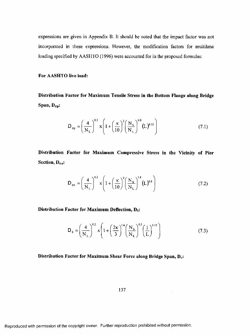
expressions are given in Appendix B. It should be noted that the impact factor was not
incorporated in these expressions. However, the modification factors for multilane
loading specified by AASHTO (1996) were accounted for in the proposed formulas:
For AASHTO live load:
Distribution Factor for Maximum Tensile Stress in the Bottom Flange along Bridge
Span, Dcrp:
op 1 + ' - Tv i o j v N w(L)'
.0.75 (7.1)
Distribution Factor for Maximum Compressive Stress in the Vicinity of Pier
Section, D<ji,:
/ ( / \V-KT A'* ^1 +
K
vTOyN ,
v N . y(L )- (7.2)
Distribution Factor for Maximum Deflection, Dg:
vN lv
0,2 f1 +
/ -KT / 2 \ 0 .1 5 ^
vN l 7(7.3)
Distribution Factor for Maximum Shear Force along Bridge Span, Dy
137
Reproduced with permission of the copyright owner. Further reproduction prohibited without permission.

2N 0.1 A
0 .1 x t O.2
L yL" ‘ NX
/
1 4"1.8 ^
/ Vl i o o j
y
(7 .4)
Distribution Factor for Maximum Exterior Support Reaction, De
^1.9^ rV TV y
X 1 +V V 300 N L y
(7.5)
Distribution Factor for Maximum Interior Support Reaction, Di:
vL“'1 +
V U O y y(7.6)
Distribution Factor for Minimum Reaction Force at the Supports, D„
D„ =\ v 6 /
+ ■0.2 N"-'N«.4 (7.7)
For Self-weight:
Distribution Factor for Maximum Tensile Stress in Bottom Flange along Bridge
Span, 9ap:
(7.8)l . lOx/
1 + f - 1f N j
0.5 ^
VU J I n l J /
138
Reproduced with permission of the copyright owner. Further reproduction prohibited without permission.

Distribution Factor for Maximum Compressive Stress in the Vicinity of Pier
Section, go„:
9 a n = 1 . 1 0 X 1 +/ \ l - 5' K '
v2y
/ -KT AN
0.5 ^
(7.9)
Distribution Factor for Maximum Deflection, gs:
Qs =1.10x 1 + (4k)' ^0.5 \
(7.10)
Distribution Factor for Maximum Shear Force along Bridge Span, gv*.
9v =1.10x 1 +v50y
(7.11)
Distribution Factor for Maximum Exterior Support Reaction, ge
9 e = l - 1 0 x 1 -----(TT3NV V L y y(7.12)
Distribution Factor for Maximum Interior Support Reaction, gi;
9i = 1 . 1 0 X 1 +5 0 ,
(7.13)
139
Reproduced with permission of the copyright owner. Further reproduction prohibited without permission.

Distribution Factor for Minimum Reaction Force at the Supports, g^:
9m =0.8 X 1 -
10 ^ 0.06 (7.14)J )
7.10 Effect of Number of Spans
In the previous sections, results from a parametric study, using three-dimensional
finite-element simulation of two-equal-span bridges were analyzed and reported.
Empirical expressions for the various distribution factors were deduced taking into
account the variations in the span length, number of lanes, number of boxes and span-to-
radius of curvature ratio. In this section, the effect of number of spans on the distribution
factors are investigated to determine whether the proposed expressions are applicable for
multiple-box girder bridges with various numbers of spans.
Four-lane three-box girder straight and curved bridges with span length of 60 m
were considered in this study. The span-to-radius of curvature ratio of the curved bridge
was taken as 1.2. Bridges with one, two, three and four spans were analyzed. Distribution
factors were calculated in each case through dividing the straining action obtained from
the 3-D finite element model by the corresponding straining action determined from the
idealized girder. It should be emphasized that the number of spans in the idealized girder
must always be the same as in the 3-D fmite-element model of the bridge analyzed.
Figure 7.29 compares the results for the distribution factor for tensile stress for all
cases considered herein. It can be observed that these factors remain almost constant for
140
Reproduced with permission of the copyright owner. Further reproduction prohibited without permission.
the various numbers of spans analyzed. The same trend was observed for both straight
and curved bridges. This confirms that distribution factor for tensile stress does not
depend on the number of spans if the distribution factor is calculated using the previously
adopted approach. Distribution factors for compressive stress for two-, three-, and four-
span bridges are plotted in Figure 7.30. It is observed that the fluctuations in the values of
distribution factors for compressive stress are less than 2%, which suggests that the
number of spans has no significant effect on the distribution factors for compressive
stress as presented. Distribution factors for deflection are illustrated for one-, two-, three-,
and four-spans bridges in Figure 7.31. The results in this Figure show that the distribution
factors for deflection for simply or continuously supported straight or curved bridges are
not significantly affected by the number of spans in the bridge.
The effect of number of spans on distribution factors for shear is presented in
Figure 7.32. No variations in the distribution factors for shear are observed for different
number of spans in the case of straight bridges. However, for curved bridges, about 5%
variations in the load distribution factor can be observed. Results for the distribution
factors for exterior reaction versus the number of spans are shown in Figure 7.33. The
trends are similar to the ones discussed for the distribution factors for shear in Figure
7.32. Similar behaviour is presented for the distribution factors for interior support
reaction in Figure 7.34. Because of the complex behaviour of the uplift reaction, some
differences in the distribution factors can be observed with different number of spans, as
shown in Figure 7.35. Such differences may be due to the changes in the location of the
uplift reaction, as governed by the loading position in the longitudinal and transverse
directions. However, it is interesting to note that the value for the distribution factors for
uplift obtained for two-span bridges can be used in estimating the uplift in straight and
141
Reproduced with permission of the copyright owner. Further reproduction prohibited without permission.
curved bridges with span length varies from 2 to 4. For curved bridges the proposed
empirical equation for distribution factors for uplift will provide conservative values
when applied to three- or four-span curved bridges.
In conclusion, it can be stated that the number of spans has an insignifieant
influence on the distribution factors. Therefore, applying the proposed empirical
equations to multiple-box girder bridges with 3 or 4 spans will lead to a fair prediction of
the actual straining action in the three dimensional bridge structures.
7.11 Effect of Inclined Webs
As a practical matter, inclined webs are often used in tub girders. The use of
inclined webs reduces the width of the bottom flange to provide for greater efficiency in
the design of bridge substructure. Their use is also aesthetically pleasing. It has been
suggested [3] that the inclination of the webs relative to a plane normal to the bottom
flange should not exceed 1 to 4. For simplicity and to reduce the number of variables in
the parametric study, webs were considered to be normal to the bottom flanges in all
bridge configurations listed in Table 6.1. In this section, the effect of inclined webs on the
load distribution factors is examined. Two bridges were analyzed herein with web slopes
having values of 0, 1/8 and 1/4. Each bridge had three lanes with span-to-radius of
curvature ratio of 0.4. The maximum results for the distribution factors were obtained
considering full and partial loading cases.
Distribution factor for tensile stress versus web slope is shown in Figure 7.36. The
results reveal differences of about 1% in these factors due to the inclination of the webs.
142
Reproduced with permission of the copyright owner. Further reproduction prohibited without permission.
It should be noted that the idealized girder consists of one-half the reduced bottom flange
and an inclined web. Figure 7.37 show the effect of web slope on the distribution factors
for compressive stress. The graph indicates that there is no noticeable variation in the
factor for the bridge with two-box girders. In the case of four-box girder bridge, increase
in the distribution factors of less than 5% is observed. The changes are quite small.
Similar trends are noted for the distribution factors for deflection, shear, exterior support
reaction, interior support reaction, and uplift reaction, shown in Figures 7.38, 7.39, 7.40,
7.41, and 7.42, respectively.
In conclusion, web slope has an insignificant effect on the load distribution
factors. However, for web design, the shear force component in the direction of the web
can be calculated by dividing the vertical shear force by the cosine of the slope angle.
7.12 Effect of Span-to-Depth Ratio
The preferred span-to depth ratio of steel box girder is not to exceed 25 [62] for
girder having a specified minimum yield stress of 350 MPa or less. With the adoption of
composite design, the preferred span-to-depth ratio for the steel box girder was relaxed to
30 [62]. The span-to-depth ratio for the composite girder, including the eoncrete deek
slab, was set at 25. Due to the curvature, the span-to-depth ratio of the steel box girder
was increased to be 25, excluding the concrete deck, for all bridges considered in this
parametric study. Accordingly, it was decided to examine the effect of span-to-depth
ration on the distribution factors.
143
Reproduced with permission of the copyright owner. Further reproduction prohibited without permission.

Two bridges with span-to-radius of curvature ratio of 0.0 and 1.2 were considered
in this study. Each bridge was a two-equal-span continuous bridge with span length of
100 m. The bridges had four-lane three-box girders each. Span-to-depth ratio of 20, 25
and 30 were considered for each bridge. Various loading cases using AASHTO live load
were applied to determine the maximum structural responses in terms of tensile stress,
compressive stress, deflection, shear force, exterior support reaction, interior support
reaction and uplift force.
Distribution factors for tensile stress are plotted versus span-to-depth ratio for
both bridges in Figure 7.43. It can be observed that these factors remain constant for the
straight bridges, with only minor variation in the results for the curved bridges. It can be
observed that as the span-to-depth ratio increase the distribution factors for tensile stress
decrease. The same trends are seen in Figures 7.44 and 7.45 for the distribution factors
for compressive stress and deflection, respectively. Therefore applying the results derived
herein, which are based on a span-to-depth ratio of 25, to bridges with span-to-depth ratio
> 25, will lead to conservative results.
Distribution factors for shear force versus span-to-depth ratio are presented in
Figure 7.46. It can be observed that for straight bridges this ratio does not influence these
factors. For curved bridges, the distribution factor for shear does increase marginally with
increase in the span-to-depth ratio. Distribution factors for exterior support reaction seem
to have the same trend as that for shear, as shown in Figure 7.47. The results for
distribution factors for interior support reaction versus span-to-depth ratio are presented
in Figure 7.48, showing no significant effect. The results for reaction distribution factors
for straight and curved bridges are given in Figure 7.49. The figure shows a decline in the
144
Reproduced with permission of the copyright owner. Further reproduction prohibited without permission.
factors with increase in the span-to-depth ratio. This means that adopting the proposed
equations for interior support reaction and uplift reaction can provide conservative values
in case of curved bridges and fairly accurate predictions for straight bridges.
7.13 Effect of Cross Bracing
Internal cross bracing are necessary to maintain the steel box shape and to reduce
transverse bending and longitudinal warping stresses in the box girder. External bracings
are also required between the boxes, as a good practice for curved bridges, to resist
torsion and distortion. Certainly, at all external brace locations, there must be a brace
placed inside the box girder to assist in the force transfer. To study the effect of cross
bracings on the structural response, a three-lane two box-girder bridge of 60-m span and
span-to-radius of curvature of 0.8 was analyzed for AASHTO truck loading. Internal
bracings, inside the boxes, and external bracings, between the boxes, were examined with
respect to their numbers between the support lines and their combined effect.
The relationship between distribution factor for tensile stress and number of cross
bracing is shown in Figure 7.50. It is evident that providing external bracing in addition to
the internal bracing slightly improves the distribution factor for tensile stress. Maximum
distribution factor for tensile stress occurs when the number of bracing is 5, at a spacing
of 10 m. Providing more cross bracings enhances marginally the distribution factors.
Figure 7.51 presents the change in the distribution factors for compressive stress versus
the niimber of cross bracings. Significant improvement in the distribution factor for
compressive stress is gained with increase in the number of bracing from 1 to 5. No
further enhancement can be realized by adding more cross bracings. Again, the graph
145
Reproduced with permission of the copyright owner. Further reproduction prohibited without permission.
shows that the presence of external bracings in addition to internal bracings does not
improve the load distribution significantly. No change is shown in the distribution factors
for deflection with increase in the number of bracings, as illustrated in Figure 7.52. It can
also be observed that external bracings do not help in reducing these factors. Figure 7.53
shows the changes in the distribution factor for shear with the number of cross bracings.
No significant effect is noted with increase of the number in cross bracings or with the
presence of external bracings. Figure 7.54 shows the same trend for the distribution
factors for exterior reaction and number of cross bracings. The influence of number of
bracings on the distribution factors for interior support reaction and distribution factors
for uplift reaction are presented in Figures 7.55 and 7.56, respectively. It can be observed
that for five bracing or more, distribution factors remain unchanged with increase in the
number of bracings. It is interesting to note that providing external bracing in addition to
internal bracing can reduce the distribution factors for uplift reaction by approximately
10%.
Figures 7.50 through 7.56 present also the effect of number of bracings on the
distribution factors for tensile stress, compressive stress, deflection, shear force, exterior
support reaction, interior support reaction, and uplift reaction for bridges under only their
self-weight. It can be observed that the graphs show similar trends to those for bridges
subjected to AASHTO live load. For number of bracings of 5 and more, the distribution
factors continue to be almost unchanged. It should also be noted that providing external
bracing maybe necessary only during casting of the concrete deck slab to prevent twisting
of the steel box girders. Thus, external bracing seems mostly unnecessary as permanent
members. However, it is good practice not to remove them since their removal can be
quite cumbersome and costly.
146
Reproducecl with permission of the copyright owner. Further reproduction prohibited without permission.

7.14 Effect of Different Type of Live Loading
The American Association of State Highway and Transportation Officials,
AASHTO 1996 [3] specifies HS20 truck semi-trailer combination in their loading. Also,
the equivalent AASHTO lane loading, consisting of a concentrated loading that is 80 kN
for bending moments and 116 kN for shear, together with a uniformly distributed load of
9.34 kN/m for all span lengths. In the parametric study conducted herein, both AASHTO
truck and lane loading were considered in order to arrive at maximum responses. In 1998,
AASHTO published a new LRFD Bridge Design Specifications [7], where the loading
consists of a design truck, or a tandem, coincident with a design lane load. The design
truck is effectively the old AASHTO truck loading. The Canadian Highway Bridge Code,
CHBDC 2000 [20] specifies two types of loading namely; CL-625 truck loading and CL-
625 lane loading. The CL-625 lane load consists of a CL-625 truck, with each axel
reduced to 80% of its normal value, together with a uniformly distributed load of 9 kN/m,
on a lane that is 3.0 m wide. In Ontario, CL-625 truck loading is replaced by CL-625-
ONT truck loading. Figure 7.57 shows the AASHTO LRFD and CHBDC truck loads. To
examine the effect of using any of these vehicular loadings on the distribution factors
derived herein, three bridges. Bridge 1, Bridge 2, Bridge 3, were analyzed using the
fmite-element method and the corresponding distribution factors were computed. The
three bridges were of two-equal-spans, continuous and horizontally curved bridges with
spans of 20, 60 and 100 m, respectively. Bridge 1 had two-lane two-box girder with span-
to-radius of curvature ratio of 0.4. Four-lane three-box girders were considered for Bridge
2 with span-to-radius of curvature ratio of 0.8. Bridge 3 was a four-lane six-box girder
brodge with a value of 1.2 for span-to-radius of curvature ratio. The multiple presence
factors specified in each code were also included in the reported results.
147
Reproduced with permission of the copyright owner. Further reproduction prohibited without permission.

Distribution factors for tensile stress are compared in Figure 7.58. It appears that
CL-625 and CL-625-ONT lane loads produce the same distribution factors. It can be
observed that AASHTO truck load gives higher values for the distribution factors for
tensile stress than those calculated on the basis of AASHTO LRFD, CHBDC and
CHBDC-ONT truck loadings. Figure 7.59 shows the variation of distribution factors for
compressive stress for bridges subjected to live loads given by the various codes. Results
based on AASHTO live loads are relatively higher than those obtained by considering the
other loadings. For shorter span length, the graphs show insignificant variation in the
distribution factors for compressive stress for all live load types examined herein.
However, for larger span length, the difference between the distribution factor for stress
based on AASHTO code and those obtained based on the other codes increases. Similar
observation can be made in Figure 7.60 for distribution factors for deflection.
Distribution factors for shear force obtained using the AASHTO, AASHTO
LRFD, and CHBDC truck loadings are compared in Figure 7.61. It can be observed that
these factors fluctuate with changes in the span length. For Bridge 1 and 3, AASHTO
truck loading gives higher results than the results corresponding to the other loadings.
However, in the case of Bridge 2, AASHTO truck loading produce lower results by
almost 5% than those obtained from CL-625-ONT. Figures 7.62 through 6.64 present the
effect of truck loadings on distribution factors for exterior, interior and uplift reactions,
respectively. In almost all cases, AASHTO truck loading provides conservative results for
design when compared to the other loadings considered herein.
148
Reproducecl with permission of the copyright owner. Further reproduction prohibited without permission.
7.15 Illustrative Design Example
Given a two-lane, two-box, curved two-equal span continuous steel girder bridge,
with a composite concrete deck slab. The box girders are simply supported at the
abutments and continuous over the pier. The bridge, designed to accommodate the
AASHTO live load (1996), has the following details: Length of one span = 45.0 m; deck
width = 9.75 m; k =L/R =0.5; deck slab thickness = 200 mm; bottom flange width =
2.4375 m and its thickness = 24 mm; web depth = 1.80 m and its thickness = 16 mm; top
steel flange width = 360 mm and its thickness = 38 mm; modulus of elasticity of steel =
200 GPa; and modular ratio = 7.4. The wearing surface is assumed to be distributed
uniformly and is = 1.2 kN W . Calculate the maximum design stresses and maximum
deflection.
The moment of inertia of an idealized girder including the concrete deck slab, I =
0.0875 m“, and the distance from the neutral axis to the bottom fibers is y = 1.277 m.
Taking the concrete and steel densities as 2,400 and 7,800 kg/m \ respectively, the total
dead load per meter length for the bridge is 20.8 kN/m. Based on this value and assuming
that the distribution for dead load is uniform, the maximum dead load positive and
negative moment in a two-45 m equal span continuous idealized girder are: 2,948 kN.m,
5,265 kN.m, respectively, and the maximum deflection and shear force are 26 mm and
585 kN, respectively. Exterior and interior support reactions are calculated as: 35land
1170 kN, respectively.
From the simple beam bending formula, the maximum tensile and compressive
stresses in the idealized girder due to the above dead load are 43.0 MPa and 76.9 MPa,
149
Reproduced with permission of the copyright owner. Further reproduction prohibited without permission.
respectively. The distribution factors for the continuous two-span bridge are now
calculated. From (7.8) and (7.9) the distribution factors for maximum tensile and
compressive stresses = 1.24 and 1.24, respectively; from (7.10) and (7.11) the distribution
factor for maximum deflection and shear force = 1.50 and 1.12, respectively. The
distribution factor for exterior, interior, and minimum support reactions obtained from
Eqs. (7.12), (7.13) and (7.14) are 1.84, 1.12, and -0.04, respectively. Based on these
distribution factors and the results from the two-span continuous idealized girder under
its own self-weight, the dead load design values for the curved continuous composite box
girder bridge according to (6.8) through (6.14) become: Op = 53.3 MPa; o„ = 95.4 MPa; 6
= 39.0 mm; V = 655 kN, Re = 646 kN; Rj = 1312 kN; R„ = -14.3 kN.
For maximum stresses, deflection, shear, and reactions due to live load on the
bridge, the procedure is to calculate first the maximum moment at the mid-span of a two-
span continuous idealized girder of 45 m span, loaded by: either a line of AASHTO
wheel loads or half the lane loading in additional to half the concentrated load. The
resulting maximum positive moment at mid-span and the negative moment in the vicinity
of the pier support are 1,270 kN.m, 1,530 kN.m, respectively, and the maximum
deflection, 5a, and shear are 13 mm and 188 kN, respectively. Maximum exterior and
interior support reactions are 149 and 320 kN, respectively. From the simple beam-
bending formula, the maximum tensile and compressive stresses, resulting from the
above moments are determined as: Opa = 18.5 MPa, and a„a = 22.3 MPa. The distribution
factors for the continuous two-span bridge are now calculated. From (7.1) and (7.2) the
distribution factors for maximum tensile and compressive stresses = 1.20 and 1.21,
respectively; from (7.3) and (7.4) the distribution factor for maximum deflection and
shear force = 1.26 and 1.36, respectively; from (7.5), (7.6), and (7.7) the distribution
150
Reproduced with permission of the copyright owner. Further reproduction prohibited without permission.
factors for exterior, interior, and minimum support reactions = 1.71, 1.34, and -0.54,
respectively. Thus, based on these distribution factors and the above results for maximum
tensile and compressive stresses, deflection, shear, and reactions for the two-span
continuous idealized girder, the design values due to live load for the box girder bridge
according to (6.1) through (6.7), become: Op == 22 MPa; a„ = 27 MPa; 6 = 0.016 m; V =
256 kN; Re = 258 kN; Ri = 429 kN; R„ = -80 kN.
Analyzing this bridge by the finite-element method, the maximum tensile and
compressive stresses obtained due to the dead load are 47 and 86 MPa, respectively, and
the maximum deflection is 34 mm. Also, for AASHTO live load, the maximum tensile
and compressive stresses are 20 and 26 MPa, respectively. The deflection due to the
AASHTO live load obtained from the finite-element analysis model is 16 mm.
Comparing the results from finite-element analysis with the ones obtained above using
the empirical formulas derived herein, it can be observed that they are in fair agreement.
For comparison, the bridge in the illustrated deign example was subjected to
AASHTO LRFD live load (1998) and also to CHBDC live load (2000). Following the
same procedure, the resulting maximum live load positive moment near mid-span and
negative moment at the interior support of a two-span continuous idealized girder were
calculated. The maximum deflection near mid-span and shear force along the span were
obtained. Also, the maximum exterior and interior support reaction forces were
calculated. The results obtained from the finite element analysis and the empirical
formulas were compared in Table 7.1. The comparisons show a fair agreement between
the results predicted by the finite element and the proposed formulas.
151
Reproduced with permission of the copyright owner. Further reproduction prohibited without permission.
7.16 Summary
The load distribution factors in continuous curved concrete deck on multiple steel
box girder bridges, subjected to AASHTO live load and dead load, were examined.
Parametric study was conducted to evaluate the maximum tensile, and compressive
stresses, deflection, shear force, exterior support reaction, interior support reaction and
minimum support reaction (uplift) using the calibrated three-dimensional fmite-element
model. Based on results obtained from the parametric study presented in this chapter, the
following conclusions can be drawn:
1. The bridge span, number of lanes, number of boxes and span-to-radius of
curvature ratio are the key parameters affecting the distribution factors.
2. Empirical expressions for the aforementioned distribution factors were deduced
for straight and curved two-span concrete-steel multiple box girder bridges. These
expressions have been shown to be reliable, simple to apply and provide
information unavailable in the current codes. They obviate the need for a rigorous
analysis involving the repeated use of three-dimensional finite element program
for different load conditions.
3. The proposed expressions for the load distribution factors can be used for the
design of equal-span continuous curved multiple box girder bridges with number
of spans varying from 2 to 4.
152
Reproduced with permission of the copyright owner. Further reproduction prohibited without permission.

4. Web slope has no significant effect on the distribution factors. Therefore, the
proposed formulas are applicable for bridges with web slope not exceeding 1 to 4.
5. The proposed expressions can be applied with confidence for bridges with span-
to-depth ratio of 25 to 30.
6. Reducing the spacing of cross bracings from 7.5 m does not improve the structural
response for the continuous curved composite multiple box girder bridges in terms
of load distribution factors. The proposed expressions are valid if internal bracings
are provided at equal intervals between the support lines with spacing not
exceeding 7.5 m.
7. The proposed expressions for distribution factors can also be used for the design
of bridges subjected to AASHTO LRFD or CHBDC live loads.
153
Reproduced with permission of the copyright owner. Further reproduction prohibited without permission.
CHAPTER VIII
Impact Factors
8.1 Introduction
In this chapter the finite element analysis of dynamic impact factors for
continuous straight and curved composite multiple-box girder bridges is described. The
main eriteria that affeet the dynamic response of curved continuous composite box girder
bridges are investigated. Methodology of the vehicle idealization, loading positions and
the vehicle speed are first presented. Then, forced vibration analysis methods are
described and compared. Stability and accuracy of the numerical methods are discussed.
Consequently, a suitable time step interval for the dynamic analysis method and damping
coefficient are selected.
Sensitivity study is conducted to decide on the unfavourable vehicle loading
conditions and the vehicle speed adapted in this dynamic analysis for such bridges.
Comparison between the mode superposition and direct integration methods is made to
choose the most effective dynamie analysis method in evaluating the impact factors. An
extensive parametric analysis is then undertaken to examine the effects of the various
aspects on the impact factors of such bridges. Results obtained from the parametric study
of 180 continuous curved composite multiple-box girder bridges are analyzed and
compared. The effects of number of lanes, number of boxes, bridge span length and the
span-to-radius of curvature ratio are discussed.
154
Reproduced with permission of the copyright owner. Further reproduction prohibited without permission.
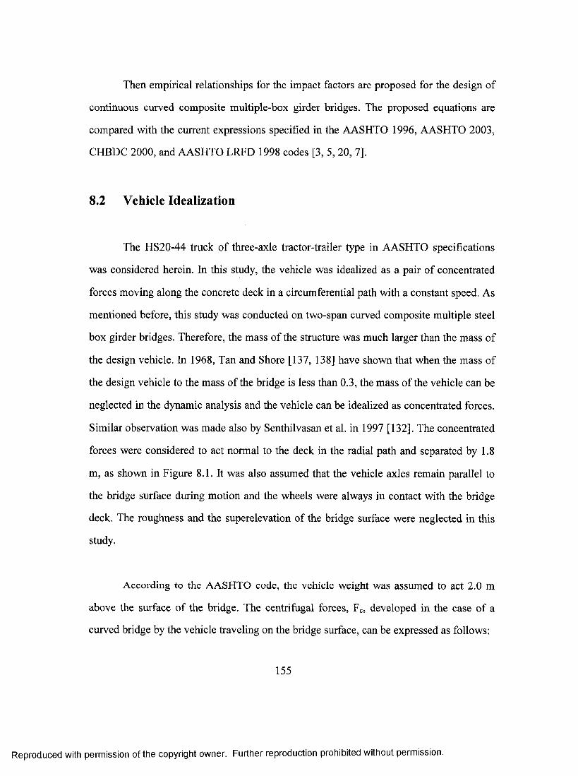
Then empirical relationships for the impact factors are proposed for the design of
continuous curved composite multiple-box girder bridges. The proposed equations are
compared with the current expressions specified in the AASHTO 1996, AASHTO 2003,
CHBDC 2000, and AASHTO LRFD 1998 codes [3, 5, 20, 7].
8.2 Vehicle Idealization
The HS20-44 truck of three-axle tractor-trailer type in AASHTO specifications
was considered herein. In this study, the vehicle was idealized as a pair of concentrated
forces moving along the concrete deck in a circumferential path with a constant speed. As
mentioned before, this study was conducted on two-span curved composite multiple steel
box girder bridges. Therefore, the mass of the structure was much larger than the mass of
the design vehicle. In 1968, Tan and Shore [137, 138] have shown that when the mass of
the design vehicle to the mass of the bridge is less than 0.3, the mass of the vehicle can be
neglected in the dynamic analysis and the vehicle can be idealized as concentrated forces.
Similar observation was made also by Senthilvasan et al. in 1997 [132]. The concentrated
forces were considered to act normal to the deck in the radial path and separated by 1.8
m, as shown in Figure 8.1. It was also assumed that the vehicle axles remain parallel to
the bridge surface during motion and the wheels were always in contact with the bridge
deck. The roughness and the superelevation of the bridge surface were neglected in this
study.
According to the AASHTO code, the vehicle weight was assumed to act 2.0 m
above the surface of the bridge. The centrifugal forces, Fc, developed in the case of a
curved bridge by the vehicle traveling on the bridge surface, can be expressed as follows;
155
Reproduced with permission of the copyright owner. Further reproduction prohibited without permission.
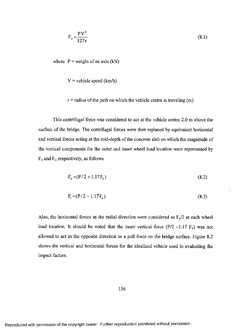
PV^(8.1)127r
where P = weight of an axle (kN)
V = vehicle speed (km/h)
r = radius of the path on which the vehicle centre is traveling (m)
This centrifugal force was considered to act at the vehicle centre 2.0 m above the
surface of the bridge. The centrifugal forces were then replaced by equivalent horizontal
and vertical forces acting at the mid-depth of the concrete slab on which the magnitude of
the vertical components for the outer and inner wheel load location were represented by
Fo and Fj, respectively, as follows
F ,= ( P /2 + 1.17FJ (8.2)
F i= ( P /2 - 1 .1 7 F J (8.3)
Also, the horizontal forces in the radial direction were considered as Fc/2 at each wheel
load location. It should be noted that the inner vertical force (P/2 -1.17 Fc) was not
allowed to act in the opposite direction as a pull force on the bridge surface. Figure 8.2
shows the vertical and horizontal forces for the idealized vehicle used in evaluating the
impact factors.
156
Reproduced with permission of the copyright owner. Further reproduction prohibited without permission.
8.3 Vehicle Loading Positions
The maximum static and dynamic responses for the compressive stresses at the
interior support were produced by applying two vehicles in the longitudinal direction, one
on each side of the interior support. Therefore, in all the cases considered in this study,
two truck loadings were positioned apart at a certain distance in the circumferential path.
This distance was selected in such a way as to produce maximum compressive
longitudinal stresses at the interior support.
In the search for the most critical loading position in the transverse direction to
obtain the impact factors, a four lane-four box curved bridge with a span length of 20 m
and a span-to-radius of curvature value of 0.4 was analyzed. Four vehicle loading
position, as shown in Figure 8.3, were considered as follows:
1. The outer lane was loaded with two vehicles, where the wheel loads were
located at a distance of 0.6 m from the curb.
2. The outer two lanes were loaded with four vehicles, where the wheel loads
for the most-outer lane were at a distance of 0.6 m from the curb.
3. The outer three lanes were loaded with six vehicles, where the most outer
wheel loads were placed near the curb as in the previous two cases.
4. All lanes were loaded with eight vehicles and the loads were positioned in
the centre of the lane.
157
Reproduced with permission of the copyright owner. Further reproduction prohibited without permission.

Some typical time histories for the curved four-lane four-box bridge with a span
length of 20 m and a radius of 50 m, as shown in Figures 8.4 to 8.7, were calculated for a
truck speed of 50 km/h. The abscissa in the figures is the distance measured from the left
end of the bridge to the front axle of the front vehicle. These figures present the time
histories of tensile stress, compressive stress, reaction force at the interior supports and
shear force at the interior support. Based on the results in these figures, it is observed that
the ease of fully loaded lanes provides the maximum dynamic response in the bridge. It
should be noted that the multiple lane load reduction factors have not been applied for
this parametric study.
8.4 Vehicle Speed
The maximum safe allowable highway speed of 100 km/h is considered in most
regions in North America. In the case of curved bridges, the maximum allowable highway
speed is restricted by the degree of the superelevation and the coefficient of side friction
force between the truck tire and the road pavement [96], and it is expressed as follows:
V = V l 2 7 r ( e + f ) (8.4)
where e = superelevation, it is considered positive if the slope of the bridge
surface is toward the centre of the curvature.
f = coefficient of side friction force between the vehicle tire and the road
surface.
158
Reproduced with permission of the copyright owner. Further reproduction prohibited without permission.

r = radius of the path along which the centre of the truck is travelling (m);
and,
V = design speed of the highway (km/h)
The superelevation of curved bridges is controlled by the design speed and the
weather conditions throughout the year at the bridge site. In severe winter condition
region, the maximum superelevation rate of 0.06 has been recommended [96]. However,
generally in most regions a maximum slope of 0.08 can be applied where high
maintenance prevails and little ice or snow accumulation is anticipated. For the purpose
of this study a value of 0.06 for the superelevation was adopted for all vehicle-loading
cases. It should be noted that applying a high rate of superelevation produees higher
allowable vehicle speed.
The friction between the truck tire and the bridge surface depend mainly upon the
type of bridge pavement, the condition of the bridge surface, the type of vehicle tire and
the vehicle speed. The maximum lateral friction influences significantly the driver’s
comfort. However, maintaining the centrifugal force on the curved bridges through lateral
friction rather than the superelevation causes discomfort for passengers. By increasing the
value of lateral friction, the allowable vehicle speed can be increased. Thus, a maximum
friction coefficient of 0.18 is considered for all cases throughout this study.
To select a suitable vehicle speed for the straight bridge, the effect of vehicle
speed was investigated for a 4l-6b-20 straight bridge. Figure 8.8 shows the tensile stress
history for three different vehicle speeds. It should be noted that with increase in the
159
Reproduced with permission of the copyright owner. Further reproduction prohibited without permission.
vehicle speed the maximum tensile stress increases. However, the change in the
maximum tensile stress is not pronounced. Similar effect is presented in Figure 8.9 for
the maximum compressive stress history. It is shown in Figure 8.10 that the increase in
the vehicle speed to 140 km/h produces a slightly higher reaction force at the interior
support. However, as seen from Figure 8.11, an insignificant change in the shear force at
the interior support occurs with increase in the vehicle speed.
In the light of above discussion, it was decided to choose a value of 120 km/h for
the maximum vehicle speed for the straight bridge. Also, an increase in the vehicle speed
with a value of almost 20 % for all eases on the curved bridges was considered. This
increase in the vehicle speed was selected for practical reasons, based on the fact that
drivers usually travel with a speed higher than the posted highway speed. Table 6.3 shows
the vehicle speeds chosen for the dynamie analysis.
8.5 Mode Superposition versus Direct Integration Method
Two types of implicit methods for dynamic analysis were discussed in Chapter 111.
A fully loaded 2l-2b-20 m straight continuous bridge was analyzed using the Mode
Superposition and Direct Integration methods.
The dynamic responses of the bridge were calculated using the case of mode
superposition method by considering 50, 100 and 200 mode shapes. These responses
were then compared to the results obtained from the direct integration method. Figure
8.12 illustrates the maximum tensile stress history for the four dynamic analysis cases.
Obviously, considering only the contribution of 50 modes, the mode superposition
160
Reproduced with permission of the copyright owner. Further reproduction prohibited without permission.
method underestimates slightly the maximum tensile stress. However, by increasing the
number of modes to 200 the estimation of the maximum tensile stress becomes very close
to the dynamic response obtained from the direct integration method. In the case of the
maximum compressive stress shown in Figure 8.13, it can be observed that the maximum
compressive stresses are close in all cases. Figures 8.14 and 8.15 depict the reaction force
and shear force history at the interior support. It can be seen that choosing only 50 modes
in the mode superposition method led to inaccurate solution. Thus, the predicted dynamic
responses of the bridge improve significantly by increasing the number of contributing
modes considered in the solution. This may be due to the phenomenon of natural
frequency clustering as reported by Galdos in 1988 [58].
As a result of the aforementioned sensitivity study and in order to obtain good
accuracy in the solution either higher number of the modes must be considered in the
solution using the mode superposition method or the analysis should be conducted using
the direct integration method. It was observed that the required time for the analysis using
mode superposition method considering higher number of modes is not less than that
needed by the direct integration method. That is due to the necessity of conducting a free
vibration analysis first in the case of mode superposition method to calculate the required
natural frequencies. Therefore, it was concluded that the direct integration method was
the most suitable method to achieve acceptable accuracy and reasonable computation
time in the dynamic analysis of the bridges.
161
Reproduced with permission of the copyright owner. Further reproduction prohibited without permission.

8.6 Stability and Accuracy
Obtaining a good approximation to the actual dynamic responses of the bridges
under consideration is the goal of the numerical integration of the finite element system
equilibrium equations. To achieve this goal, all system equilibrium equations
significantly contributing to the dynamic responses of the structure must be integrated to
a high precision. This means that the selection of the time step, At, is crucial to the
accuracy and the stability of the solution. Theoretically, the time step At would have to be
almost T/10 [12], where T is the smallest period. However, this assumption is not
required in practice. Generally, the dynamic response of a structure is predicted by
inclusion of only the first few modes. Thus, the dynamic response can be determined
accurately by integrating only the first few effective modes. Thus, the choice of At would
be selected according to the smallest period for the most contributing modes instead of
the smallest period for all modes of the structure.
The implicit method used by ABAQUS/Standard is unconditionally stable. This
means that for any time step At, the estimated solution for any initial condition does not
grow without bound. In addition, the accuracy in the predicted dynamic response of the
structure can be preserved in the unconditionally stable integration method by choosing
the time step At small enough that the response in all modes that contributed significantly
to the total structural response is determined accurately. However, it should be noted that
the other model response components are not calculated precisely but the produced errors
are not critical for the obtained dynamic response.
162
Reproduced with permission of the copyright owner. Further reproduction prohibited without permission.

As verification of the previous considerations, two continuous curved bridges,
with L/R = 0.4, were analyzed. Both bridges were fully loaded with truck loading. The
first bridge had a span length of 20 m while the second one had a span of 60 m. Dynamic
responses for both bridges were obtained at various time steps using the direct integration
method. For the 20 m span bridge, the dynamic responses using time steps with values of
0.002, 0.010, 0.015 and 0.020 seconds were predicted. However, in the case of 60 m span
bridge, values of the time steps considered in the dynamic analysis were 0.005, 0.014 and
0.020 seconds.
Tensile and compressive stress histories are plotted in Figures 8.16 and 8.17. It is
clear that the dynamic responses for the tensile and compressive stresses obtained using a
value of 0.002 seconds for At are higher by about 6% than those calculated for larger time
steps. However, the difference in the results is not significant in both responses. The
results of the reaction force and the shear force are presented in Figures 8.18 and 8.19. It
should be noted that carrying out the integration of the equilibrium equations for the
maximum reaction force using a time step with a value of 0.002 seconds is higher by
about 14% than those predicted using a larger time steps. However, this effect of the time
step on the maximum shear force is less than 1%. Similar dynamic responses for the 60
m-span bridge are illustrated in Figures 8.20 to 8.23. It is interesting to note that there is
no marked effect of the time step on the tensile stress history. The dynamic response for
compressive stress, reaction force and shear force are somehow affected by reducing the
time step. However, the differences in estimating the maximum values are less than 5%.
Cleary, reducing the time step would provide more accuracy in the prediction of
the dynamic response of the bridges. However, it will increase dramatically the analysis
163
Reproduced with permission of the copyright owner. Further reproduction prohibited without permission.

time and consequently the cost. Therefore, as a result of the previous investigations of the
two bridges the time step with a value of 0.020 seconds was selected in the case of 60 m,
80 m, and 100 m span length. On the other hand, a value of 0.01 seconds was applied in
the dynamic analysis of 20 m and 40 m span length bridges.
8.7 Damping Effect
It is well known that the magnitude of oscillation of a structure decreases until the
oscillations stop due to energy dissipation. This energy dissipation in a structure is called
damping. By applying the general direct integration method provided in
ABAQUS/Standard, called Hilber-Hughes-Taylor operator, an artificial damping is
introduced. This damping is purely numerical. The a-parameter introduces damping that
grows with the ratio of the time step to the period of vibration of a mode. The parameter,
a, can take any value from 0, which gives no artificial damping, to -0.33 which provides
the maximum artificial damping available from this operator.
The dynamic analysis of 3l-3b-60 m straight bridge was conducted. The histories
of tensile stress, compressive stress, reaction force and shear force at the interior support
were calculated for a = 0, -0.05, and -0.33. The damping effect on the tensile stress and
reaction force are shown in Figures 8.24 and 8.25, respectively. It should be noted that the
maximum results of all the dynamic responses were only slightly different for all the
above artificial damping values. Therefore, a value of 0.0 for a was selected in all cases
considered in the parametric study.
164
Reproduced with permission of the copyright owner. Further reproduction prohibited without permission.
8.8 Dynamic Impact Factor
Maximum vertical loads caused by a travelling vehicle across a bridge will often
exceed those exercised by an equivalent static vehicle due to the dynamic effects [37].
This increase in the vertical loads has commonly known as Impact Factor, I, or Dynamic
Load Allowance. According to AASHTO Guide Specifications, the dynamic design
values can then be obtained from the following relationship
Maximum dynamic response = Maximum static response (1 + 1) (8.5)
While the impact factor considered in this study is defined as
I (o/o) X 100 (8.6)Rs
where Rd = maximum dynamic response
Rs = maximum static response
Dynamic and static analyses were conducted on each bridge for the same applied
loads in both analyses. Maximum dynamic and static responses for tensile stress near the
mid span, compressive stress at the interior support, deflection near the mid span, reaction
force at the exterior supports, reaction force at the interior support, uplift reaction, shear
force at the exterior support and shear force at the interior support were determined for all
bridges considered herein. Thus, impact factors were calculated by applying Equation 8.6
for the 180 bridges analyzed in this parametric study. In the longitudinal direction of the
165
Reproduced with permission of the copyright owner. Further reproduction prohibited without permission.
bridge, two trucks for each lane were applied. The trucks were travelling apart from each
other with various distances depending upon the span length. The distances between the
trucks were chosen in such a way as to produce maximum negative moment on the
interior support for a bridge. The vehicle speeds considered in this study for all bridges
are presented in Table 6.3.
As previously mentioned in section 8.3, the case of fully loaded lanes with truck
loading, in general, produces the maximum straining actions in the structure. Therefore,
this loading case is used for all bridges analyzed in the parametric study to evaluate their
impact factors. It should be mentioned that the time required to obtain the dynamic
response of one bridge on a Solaris 9 Sun Fire 4800 with 4 CPUs and 4 GB memory
using ABAQUS/Standard is more than four days in some cases.
8.9 Parametric Study
The literature suggests that the impact factor of vehicle loads travelling on a
bridge depends upon a wide range of parameters. In this study the following four main
factors were selected to have the most influence on the dynamic behaviour of continuous
curved composite multiple-box girder bridges; namely: 1) Number of bridge lanes; 2)
Number of bridge boxes; 3) Bridge span length; and, 4) Span-to-radius of curvature ratio.
In the parametric study, all these parameters were thoroughly investigated. In the
following section, results are presented in graphs and finally expression for impact factors
are derived.
166
Reproduced with permission of the copyright owner. Further reproduction prohibited without permission.
8.9.1 Effect of Number of Lanes
In this study, the number of lanes considered herein was two, three and four. Since
the number of lanes is a clear indication of the variation of the bridge width, this
parameter is considered as a key factor in the bridge geometry and consequently, one that
significantly influences the bridge behaviour under dynamic loads. To investigate the
effect of number of lanes on the impact factors a four-box bridge with a span length of 20
m was analyzed for moving vehicles.
Impact factor for tensile stress is plotted against the number of lanes in Figure
8.26. The graph shows that the values of impact factor do not follow a certain pattern for
bridges with increase in the number of lanes. For curved bridges, it can be observed that
there is no general trend for the impact factors with change in the number of lanes.
Similar observations were made for impact factors for compressive stress, deflection,
shear, and reaction. Based on the above results, it is interesting to note that the number of
lanes, and hence the bridge width, does not have a patterned effect on the impact factors
for continuous curved composite multiple-box girder bridges.
8.9.2 Effect of Number of Boxes
In this section, the effect of the number of boxes on the impact factors for straight
and curved bridges is investigated. Two lanes-20 m bridges with L/R= 0.0, 0.1, 0.2 and
0.4 are considered in this study.
167
Reproduced with permission of the copyright owner. Further reproduction prohibited without permission.
As shown in Figure 8.27 the impact factors for tensile stress are plotted against
the number of boxes. It can be observed that the calculated results for the impact factors
for straight bridges increase slightly with increasing the number of boxes. However, in
the case of curved bridges the impact factors do not change in any systemic manner with
the number of boxes. In general, the effect of number of boxes on the impact factors for
continuous curved concrete deck on multiple steel box girder bridges does not follow any
pattern. Basically, the variation of the impact factor values with number of boxes is not
pronounced in most cases.
8.9.3 Effect of Span Length
The effect of the bridge span length on the impact factors for tensile stress is
shown in Figure 8.28. For straight bridges, it is clear from this figure that the impact
factors decrease with increasing span length of the bridge. Similar observations are
obtained for impact factors for compressive stress, deflection, shear, and reaction. In
summary, for straight bridges, the impact factors for tensile, and compressive stresses,
exterior support, and interior support reactions decrease with increase in the span length.
8.9.4 Effect of Span-to-Radius of Curvature Ratio
Impact factor values for two selected bridges with span length of 20 m and 40 m,
respectively, were calculated. Each bridge had two lanes and two boxes. The vehicle
speed eonsidered in this examination varied according to the radius of curvature in each
case. The effect of span-to-radius of curvature ratio on the impact factor for tensile stress
is presented in Figure 8.29. While no definite trend is observed in the case of 2/-26-20
168
Reproduced with permission of the copyright owner. Further reproduction prohibited without permission.

bridges, bridges with span length of 40 m show a uniform increase in the impact factor.
Similar behaviour is observed for the impact factors for compressive stress, deflection,
shear, and reaction as those obtained for the impact factors for tensile stress for both
bridges. Thus, the effect of the span-to-radius of curvature on the impact factors of curved
or straight bridges does not follow any pattern of behaviour.
8.10 Expressions for Impact Factor
In the previous sections, the effects of several variables on the impact factors in
straight and curved continuous concrete deck on multiple steel box girder bridges were
examined using the finite element computer program ABAQUS/standard. The maximum
selected design speed as shown in Table 6.3 and the full loaded lane condition were
applied for all bridges considered in this parametric study. Impact factor results were
plotted versus the number of lanes, munber of boxes, bridge span length and the span-to-
radius of curvature ratio. In some cases, the impact factors have shown a clear trend with
regard to a specific variable. However, in many cases no pattern was observed. As
expected, impact factors for stresses, deflection, reaction forces and shear forces have
been influenced differently by each of the above variables. This is due to the complicated
structural dynamic behaviour of continuous curved composite multiple-box girder
bridges.
Previous researchers often related the fundamental frequency of a bridge to its
impact factor [108, 22]. Also, bridge span length was considered as the most important
influential factor in estimating impact factors in most codes [3]. Thus, the next section
deals with impact factors expressed as a function of each of the following: the
169
Reproduced with permission of the copyright owner. Further reproduction prohibited without permission.
fundamental frequency; and, the bridge span length. In addition, while the span-to-radius
of curvature ratio of a bridge plays a vital role in the overall structural dynamic behaviour
of bridges, expressions for impact factors are also given in terms of the span-to-radius of
curvature ratio.
The main objective of this study is to proposed simplified and practical
expressions for impact factors. Therefore, upper bound values for the impact factors in all
cases were established as follows.
8.10.1 Impact Factor as a Function of the Fundamental Frequency
The impact factor results for all analyzed straight and curved bridges for tensile
stress, compressive stress, deflection, exterior support reaction, interior support reaction,
uplift, shear at the exterior support and shear at the interior support are plotted against the
bridge ftmdamental frequencies as shown in Figures 8.30 though 8.37. It is interesting to
note that there is a difference between straight and curved bridges for low frequencies.
However, results for straight bridges with f =5 Hz fall into the range of values for the
curved bridges with the same frequency. That is mainly due to the fact that small span-to-
radius of curvature ratio was assumed for short span bridges. Impact factors are presented
separately for straight bridges to emphasis at the change in the impact factor values due to
the bridge curvature. Expressions based on the upper bovmd values for the impact factors
for curved bridges were derived as follows:
1) Impact Factor for Tensile Stress (Figure 8.30)
170
Reproduced with permission of the copyright owner. Further reproduction prohibited without permission.
Ip = 2 3 -2 .5 f (8.7)
2) Impact Factor for Compressive Stress (Figure 8.31)
I „ = 2 7 - 2 . 4 f (8.8)
3) Impact Factor for Deflection (Figure 8.32)
I d = l l + 0.5f (8.9)
4) Impact Factor for Exterior Support Reaetion (Figure 8.33)
I , e = 2 2 - f (8.10)
5) Impact Factor for Interior Support Reaction (Figure 8.34)
I , i= I8 + 0.5f (8.11)
6) Impact Factor for Uplift Reaction (Figure 8.35)
I u = 1 6 0 (8 .1 2 )
7) Impact Factor for Shear at Exterior Support (Figure 8.36)
I s e = 1 6 - 2 f (8.13)
171
Reproduced with permission of the copyright owner. Further reproduction prohibited without permission.
8) Impact Factor for Shear at Interior Support (Figure 8.37)
I s i = 3 7 - 4 f (8.14)
where f is the fundamental frequency in Hz.
8.10.2 Impact Factor as a Function of Bridge Span Length
The values of impact factors are presented as function of the bridge span length in
Figures 8.38 through 8.45. The available expressions for impact factors given in
AASHTO 1996, AASHTO 2003, CHBDC 2000 and AASHTO LRFD 1998 guide
specifications [3, 5, 20, 7] are also presented for comparison. Straight bridge results are
first plotted separately to show the variations in the impact factor values when
considering the results from curved bridges. Upper bound impact factors as a function of
the curved bridge span length were deduced as follows:
1) Impact Factor for Tensile Stress (Figure 8.38)
Ip =21 (8.15)
2) Impact Factor for Compressive Stress (Figure 8.39)
I „ = 2 5 (8.16)
3) Impact Factor for Deflection (Figure 8.40)
172
Reproduced with permission of the copyright owner. Further reproduction prohibited without permission.
Id =13 (8.17)
4) Impact Factor for Exterior Support Reaction (Figure 8.41)
h = 2 0 (8.18)
5) Impact Factor for Interior Support Reaction (8.42)
I r i =2 0 (8.19)
6) Impact Factor for Uplift Reaction (Figure 8.43)
lu = 160 (8.20)
7) Impact Factor for Shear at Exterior Support (Figure 8.44)
I s e = 2 4 ( 8 . 2 1 )
8) Impact Factor for Shear at Interior Support (Figure 8.45)
Isi = 34 (8.22)
173
Reproduced with permission of the copyright owner. Further reproduction prohibited without permission.
8.10.3 Impact Factor as a Function of Span-to-Radius of Curvature Ratio
In this section, results of the impact factors are presented as functions of span-to-
radius of curvature ratio in Figures 8.46 to 8.53. Considering only this parameter, upper
bound expressions were developed for the impact factor values as follows:
1) Impact Factor for Tensile Stress (Figure 8.46)
l p = 1 0 ( l + L / R ) (8.23)
2) Impact Factor for Compressive Stress (Figure 8.47)
1 „ = 5 ( 4 + L/R) (8.24)
3) Impact Factor for Deflection (Figure 8.48)
Id = 1 4 - 3 (L /R ) (8.25)
4) Impact Factor for Exterior Support Reaction (Figure 8.49)
Ire = 20 (8.26)
5) Impact Factor for Interior Support Reaction (Figure 8.50)
l,i = 2 2 - 1 0 (L/R) (8.27)
174
Reproduced with permission of the copyright owner. Further reproduction prohibited without permission.
6) Impact Factor for Uplift Reaction (Figure 8.51)
I„ =190-135(L/R) (8.28)
7) Impact Factor for Shear at Exterior Support (Figure 8.52)
I,, = 2 9- 13 (L/R) (8.29)
8) Impact Factor for Shear at Interior Support (Figure 8.53)
I,i = 1 6 -1 5 (L /R ) (8.30)
Since all values obtained from the three equations for impact factors for any
structural quantity are upper bound, the designer is free to use any of the equations for a
safe design.
8.11 Summary
The direct integration method was applied to calculate the dynamic response of
continuous straight and curved composite multiple-box girder bridges. A suitable time
step At was selected in such a way to maintain low computational cost for the analysis
without jeopardizing the accuracy of the solution. Finite element models of bridges were
subjected to an idealized vehicle loading in all bridge lanes. The vehicle speed was
selected as 120 km/h for the straight bridges. However, for curved bridges the vehicle
speed was reduced according to the span-to-radius of curvature ratios. It should be noted
175
Reproduced with permission of the copyright owner. Further reproduction prohibited without permission.

that the chosen vehicle speeds are in all cases higher than the maximum allowable
highway speed for safety reasons. Based on the results of the dynamic analysis carried out
in the parametric study, the following conclusions on the impact factors of these bridges
can be made:
1. No discernible influence of the number of lanes and boxes on the impact
factors was observed.
2. In the case of straight bridges, the impact factors for tensile, and
compressive stresses, deflection, exterior, and interior support reactions,
decreased, in general, with increase in the span length. However, this trend
was not the case for curved bridges.
3. The span-to-radius of curvature ratio has a measurable influence on the
magnitude of the impact factors regardless of the span length of the bridge.
4. Impact factors for tensile and compressive stresses, deflection, exterior,
and interior support reactions for straight bridges increase with higher
fundamental frequencies. However, this trend was not preserved when the
results of impact factor for curved bridges were considered.
5. Formulas given in AASHTO 1996 [3] underestimate, in most cases, the
impact factors for bridges with large span lengths.
176
Reproduced with permission of the copyright owner. Further reproduction prohibited without permission.

6. Impact factors for uplift reaction are generally underestimated by all
current North American Codes.
7. Both AASHTO LRFD and AASHTO 2003 [5, 7] overestimate the impact
factors for tensile, and compressive stresses, deflection, reactions, and
shear at the exterior support.
8. Impact factors based on CHBDC 2000 [20] appear to be the closest values
to those predicted by the proposed expressions. However, this Code
underestimates the impact factors for the uplift reaction and shear at the
interior support.
9. Given the scattered nature of most of the impact factors values obtained, it
was necessary to develop the impact factor expressions as upper bound
solutions from all results gathered from the parametric study.
177
Reproduced with permission of the copyright owner. Further reproduction prohibited without permission.

CHAPTER IX
Fundamental Frequency
9.1 Introduction
There are several factors, which influence the dynamic characteristics of
continuous curved concrete deck-on-multiple steel box-girder bridges. In order to
consider some of factors for calculating the dynamic response, they need to be assembled
into a form that is convenient. This is normally achieved by characterizing a bridge
mainly in terms of its natural frequency and mode shape. By knowing the value of
fundamental frequency of a bridge, impact factors can be evaluated. Since most heavy
vehicle frequencies occupy a relatively narrow frequency band in practice, 1.5 to 4.5 Hz,
it is preferred to design bridges in such a manner as to avoid this critical range, if at all
possible. In addition, due to bridge vibration, the dynamic deflection can cause
discomfort to pedestrians using the bridge. It has been known that the human body tends
to react more to torsional oscillations than flexural ones.
Accordingly, it is crucial to offer a reliable method to evaluate accurately the
fundamental frequencies of multiple box girder bridges. Therefore, in this chapter, the
results of extensive analytical investigations on the vibration characteristics of continuous
curved concrete deck-on-multiple steel box-girder bridges are generated. The analysis of
the three-dimensional bridges was performed using the finite-element method. Empirical
expressions were then derived from these results to evaluate the fundamental frequencies
178
Reproduced with permission of the copyright owner. Further reproduction prohibited without permission.
of such bridges. The influences of bridge spans, number of lanes, number of boxes and
span-to-radius of curvature ratios on the fundamental frequencies were examined.
Furthermore, the effects of number of spans, span-to-depth ratio, end-diaphragm
thickness and number of cross-bracings were also investigated. Forced vibration analysis
was also conducted to examine the peak acceleration due to AASHTO truck loading
passing along the bridge. Effects of truck speed, end-diaphragm thickness and number of
cross-bracings on the peak acceleration were also studied.
9.2 Effect of Span Length
The effect of bridge span length is considered as a major factor affecting the
fundamental frequencies of bridges. Results obtained from 180 continuous curved
concrete deck-on-multiple steel box-girder bridges were plotted in Figure 9.1(a). As
illustrated in the graph, flmdamental frequencies decrease considerably with increasing
bridge span length. It is interesting to observe, however, that for eaeh span length, the
values of the fundamental frequencies vary within a maximum range of 20 %. These
variations are caused by the effects of other parameters, such as number of lanes, number
of boxes or L/R ratios. Mode shapes were also derived for all bridges. For straight
bridges, the first mode shape is always purely flexural, which is not the case for curved
bridges. Figure 9.1(b) shows the mode shapes of 3/-2Z> bridges with L/R ratio of 0.6. It
appears that the contribution of the torsional effects to the first mode shape of continuous
curved multiple box-girder bridges decreases with inerease in the span length. In that case
the flexural effect becomes more predominant.
179
Reproduced with permission of the copyright owner. Further reproduction prohibited without permission.
9.3 Effect of Number of Lanes
Four-box 20-m and 60-m bridges with L/R ratio of 0.4 were considered to
illustrate the effect of the number of lanes on the fundamental frequencies, as shown in
Figure 9.2(a). It is observed that the fundamental frequencies of 20-m bridges decrease by
almost 7% when the number of lanes increases from 2 to 4. However, in the case of
bridges with 60-m span length, the fundamental frequencies remain almost unchanged. It
is obvious from the results of for all bridges considered in this study that the number of
lanes has no pronounced influence on the fundamental frequencies. Regardless of the
number of lanes, the first mode shape for a straight bridge is purely flexural. However, for
curved bridges the torsional effects influence the first mode shapes. Figure 9.2(b) shows
that the torsional influence in the first mode increases slightly by increasing the number
of lanes.
9.4 Effect of Number of Boxes
The influence of number of boxes on the fundamental frequencies is presented in
Figure 9.3(a). Three-lane straight bridges with span lengths of 20 and 60 m and having
different number of box girders were analyzed. The results shown revealed that
increasing the number of boxes only slightly enhances the fundamental frequencies of the
bridges. An increase in the fundamental frequency of bridges with 60-m of about 7% was
noted when the number of boxes increased from 2 to 5, with almost 2% in the case of
bridges with 20 m span lengths. It should be noted that the effect is not significant due to
the fact that there is no change in the width of the bottom flange even when the number of
boxes is increased. The increase is in the number of webs. Results not shown herein
180
Reproduced with permission of the copyright owner. Further reproduction prohibited without permission.
reveal that the number of boxes had no effect on the first mode shape of straight bridges.
However, it seems that increasing the number of boxes in curved bridges increases the
torsional effect on the first mode shape as shown in Figure 9.3(b). This may be attributed
to a decrease in the torsional stiffness with inerease in the number of boxes for the same
flexural stiffness.
9.5 Effect of Span-to-Radius of Curvature Ratio
The relationship between the fundamental frequency and span-to-radius of
curvature ratio (L/R) of three-lane two-box bridges with span lengths of 60 and 100 m are
presented in Figure 9.4(a). The graph shows that L/R ratio has a signifieant effeet on the
fundamental frequencies. Increasing the L/R ratio significantly decreases the fundamental
frequency. For instance, the fundamental frequency of bridges with span length of 60 m
decreased by about 29% when L/R ratio increased from 0 to 1.2, and by about 32% in the
case of bridges with span length of 100 m. It can be observed that first mode shapes of
curved bridges are also affected considerably by increasing the L/R ratio. For straight
bridges, the first mode shape is purely flexural for all bridge span lengths. However, this
behaviour changes by introducing curvature in the bridge geometry, where the torsional
effects play a significant part. Figure 9.4(b) shows the mode shapes of 3/-2Z>-100 bridges
with span-to-radius ratios of 0 and 1.2, showing the effect of torsion due to the bridge
curvature.
181
Reproduced with permission of the copyright owner. Further reproduction prohibited without permission.

9.6 Empirical Expressions for Fundamental Frequency
Based on the results generated from the parametric study of continuous straight
concrete deck-on-multiple steel box-girder bridges, the following simplified empirical
equation was deduced for the fundamental frequency, fj:
94f ^ = - Hz (9.1)
The accuracy of this expression is within 3% for all straight bridges considered in
this parametric study regardless of the number of boxes or lanes. It should be noted that
same expression is valid for simply-supported straight bridges [119].
Since bridge curvature significantly affect the fundamental frequencies, a
modification factor is introduced in Eq. 9.1 to account for the curvature effect. The
modified expression for the fundamental frequency of curved bridges, fc, is given as:
f, = p . f, Hz (9.2)
where q is a modification factor defined as:
q = l - 0 . 0 71.5 f N , . L ] 0.3
u . N , J (9.3)
where L is the centreline arc length of the curved bridge in one span in meters; R is the
radius of curvature of the bridge centreline; Nb is the number of boxes; and Nl is the
182
Reproduced with permission of the copyright owner. Further reproduction prohibited without permission.
number of lanes. It should be noted that the number of lanes and number of boxes do
affect to some degree the fundamental frequency of curved bridges. This is reflected in
Eq. 9.3. Equation 9.2 is quite accurate in predicting the fundamental frequency for two-
span curved concrete deck on multiple steel box girder bridges included in the parametric
study with an error not exceeding 3%. It should be noted that Eq. 9.2 applies only to span-
to-depth ratios of 25. For different such ratios, another equation was developed as shown
in a forthcoming section.
9.7 Comparison with Flexural Beam Theory
Flmdamental frequency of a continuous beam girder can be evaluated using the
flexural beam theory, as follows;
J - Hz (9.4)2L V m
where m is the total mass per unit length of the beam girder; I is the flexural moment of
inertia of the beam girder; L is the span length of the beam girder; and E is the modulus
of elasticity of the girder material. In order to include the curvature effect, Heins and
Sahin [68] had evaluated the fundamental frequency of curved box girders using the
differential equations of motion based on Vlasov’s thin-walled beam theory assuming that
the entire cross section at the supports would not twist. In practice, box-girders in bridges
are supported only at the bottom flanges underneath the webs. Accordingly, the end cross-
section of a bridge at the support line becomes more flexible than assumed, particularly
for bridges with small span-to-depth ratios.
183
Repro(juG8(j with permission of the copyright owner. Further reproctuction prohibitect without permission.
In this parametric study, results obtained from the three-dimensional fmite-element
models were normalized by the fundamental frequencies for a similar straight girder. The
section properties of the straight girder were taken as those obtained form the
corresponding bridge with span length equal to the centre line arc length. The
fundamental frequency of the straight girder can be evaluated using Eq. 9.4. Modification
factors were applied to the fundamental frequency of the straight girder to develop the
following empirical expression for the fundamental frequency, f, of two-span curved
concrete deck-on-multiple steel box-girder bridges:
f=0.94.p.fbeam Hz (9.5)
where p and fbeam are evaluated from Eqs. 9.3 and 9.4, respectively. A comparison of the
results using Eq. 9.5 and the finite element solution for two-span curved concrete deck-
on-multiple steel box-girder bridges shows good correlation, with the errors not
exceeding 8% for all the bridges considered in the parametric study.
9.8 Effect of Span-to-Depth ratio
The value of span-to-depth ratio of 25 is preferred when the yielding stress of the
steel does not exceed 350 MPa. For yielding stress beyond 350 MPa, span-to-depth ratio
can be relaxed to 30 [62]. Until now, all bridges considered in this parametric study had a
span-to-depth ratio of 25. However, since the fundamental frequencies of bridges are
affected by this ratio three different values of span-to-depth ratios of: 20, 25 and 30, were
investigated. Four-lane three-box bridges with span length of 100 m were examined in a
sensitivity study. Span-to-radius ratios of 0.0, 0.6 and 1.2 were considered.
184
Reproduced with permission of the copyright owner. Further reproduction prohibited without permission.

Figure 9.5 shows the effect of span-to-depth ratio on the fundamental frequency. It
is obvious that the fundamental frequencies decrease almost linearly with increase in the
span-to-depth ratio, irrespective of the degree of curvature considered herein. For
example, in the case of straight bridges, the fundamental frequency decreased by more
than 30% when span-to-depth ratio increased from 20 to 30. Similarly, the fundamental
frequencies of curved bridges declined significantly by almost 28%. Thus, these results
show that changing the span-to-depth ratio affects considerably the fundamental
frequency for continuous curved concrete deck-on-multiple steel box-girder bridges. It
should be noted that the applieation of the empirical Eq. 9.2 is limited to bridges with
span-to-depth ratio of 25. On the other hand, Eq. 9.5 can be applied to bridges with
various span-to-depth ratios. Table 9.1 shows the results obtained from the three-
dimensional finite-element models correlating quite well with the results estimated by
empirical Eq. 9.5 for various span-to-depth ratios.
9.9 Effect of End-Diaphragm Thickness
Figure 9.6 shows the effect of end-diaphragm thickness on the first four natural
frequencies for continuous 2l-2b bridges with span length of 40 m and L/R ratio of 0.4.
From the results shown it is apparent that end-diaphragm thickness has no effect on the
flexural modes. However, providing end-diaphragms over the bridge supports enhances
significantly the torsional effects and accordingly increases the third and fourth natural
frequencies. As the end-diaphragm thickness increases to 10 mm, significant
improvement in the torsional modes is obtained. Nevertheless, any further increase in the
end-diaphragm thickness produces very little enhancement in the torsional modes.
Therefore, providing end-diaphragm at the support line inside the boxes with the required
185
Reproduced with permission of the copyright owner. Further reproduction prohibited without permission.
minimum practical thickness specified in the codes is quite adequate to improve the
torsional frequency modes for continuous curved multiple box girder bridges.
9.10 Effect of Cross Bracings
The effeet of internal and external cross bracings on the natural frequencies of 3/-
3b bridges with span length of 60 m and L/R ratio of 0.8 is illustrated in Figure 9.7.
Different numbers of cross bracings were provided in each span and the first four
frequencies are presented. Clearly, the first and second frequencies of the bridges are not
affected by the presence of internal cross bracings or internal and external cross bracings.
This is because the first and second natural modes are basically flexural modes. The
contribution of the torsional effect becomes more dominant in the third and fourth modes.
Thus, it is shown that the presence of cross bracings enhances dramatically the third and
fourth natural frequencies. Providing both internal and external cross bracings improves
even more the torsional modes. It can be observed, also, that a minimum of five cross
bracings, with 10 m spacing (as specified in the bridge code) is necessary to achieve the
maximum enhancement in the torsional frequencies. Increasing the number of cross
bracing beyond 5 does not appear to contribute to the dynamic characteristics of such
bridges.
9.11 Effect of Number of Spans
The relationships between the number of spans and the first four natural
frequencies are plotted in Figure 9.8 for straight and curved bridges with four lanes and
three boxes. The bridges have span length of 60 m with number of spans 2, 3 and 4. It is
186
Reproduced with permission of the copyright owner. Further reproduction prohibited without permission.

interesting to observe that the value of the first natural frequency remain constant with
change in the number of spans for both straight and curved bridges. This means that all
previous empirieal expressions obtained for two-span bridges may be applied to three-
and four-span bridges. However, it should be noted that for all the bridges analyses the
span lengths were equal. It is also observed that the third and fourth natural frequency
results decrease with an increase in the number of spans.
9.12 Forced-Vibration Analysis
The forced-vibration analysis was carried out to study the effeets of truck speed
and span-to-radius of eurvature on the peak acceleration at the bridge deck. Two different
transverse positions of AASHTO truck loading were considered in the forced vibration
analysis of 2/-36-60 bridges with L/R ratios of 0, 0.4, 0.6 and 1.2. Furthermore, the
effects of end-diaphragm thickness and number of cross-bracings on the peak acceleration
were also examined in this study. In all cases, full and outer lane truek loadings were
considered.
9.12.1 Effect of Vehicle Speed
The maximum peak accelerations for 2l-3b-60 bridges with span-to-radius of
curvature ratio of 0.6 were plotted against the vehicle speed in Figure 9.9. Various vehicle
speeds, 50, 60, 80 and 120 km/h, were considered in the analysis. It ean be observed that
the accelerations are higher, generally, for fully loaded lanes with two trueks traveling in
the eentre of their lanes. The peak acceleration occurred in both loading cases for a
vehiele speed of 60 km/h. Inereasing the vehicle speed above 80 km/h, the peak
187
Reproduced with permission of the copyright owner. Further reproduction prohibited without permission.
acceleration increased. However, for vehicle speed 120 km/h, the peak acceleration was
lower than those obtained for vehicle speed of 60 km/h.
9.12.2 Effect of Span-to-Radius of Curvature Ratio
The effect of span-to-radius of curvature ratio of 2/-3&-60 bridges on the peak
acceleration is illustrated in Figure 9.10. It is clear that increasing the bridge L/R ratio
affects significantly the maximum peak acceleration values. The maximum peak
acceleration increases by approximately 150 % when the L/R ratio is increased from 0 to
1.2. Full and partial truck loading cases showed similar trend. However, the full truck
loading case produced higher values of peak acceleration than those calculated for partial
truck loading case.
9.12.3 Effect of End-Diaphragm Thickness
Two-lane three-box bridges with span length of 60 m and span-to-radius ratio of
1.2 were examined in this study. Various end-diaphragm thicknesses were considered. A
vehicle speed of 120 km/h was maintained in all cases. Figure 9.11 presents the
relationship between the maximum peak acceleration and diaphragm thickness. The
results show that providing end-diaphragm reduces the peak acceleration considerably,
particularly for full truck loading case. Also, increasing the diaphragm thickness beyond
10 mm has no significant effect on the peak acceleration for both loading cases.
188
Reproduced with permission of the copyright owner. Further reproduction prohibited without permission.
9.12.4 Effect of Number of Cross Bracings
Two types of cross bracings were selected for this study. The first type is made of
internal bracings, inside the boxes, while the second one is made of internal and external
crossing bracing, i.e. inside and between and the boxes. The 2/-3Z>-60 bridges with span-
to-radius of curvature ratio of 1.2 were examined in this investigation. One, five, eight,
and eleven cross bracings, a vehicle speed of 120 km/h and full truck loading were
considered in analysis. Figure 9.12 shows the variation of peak acceleration against the
number of cross bracings. It can be observed that the peak accelerations for both cross
bracing configurations decrease with increasing the number of bracing from 1 to 5. The
reduction in peak acceleration is about 65% for the case of internal bracing only and 14%
for the case of external and internal bracing. Cleary, increasing the number of bracings
beyond 5 has an insignificant effect on the peak acceleration.
9.13 Summary
A free-vibration analysis of continuous curved composite multiple box-girder
bridges was conducted using a three-dimensional finite-element model. A parametric
study was undertaken to scrutinize the effects of various parameters on the natural
frequencies and the corresponding mode shapes. A forced-vibration analysis was then
conducted to examine the effect of some parameters on the peak acceleration values.
Based on this study, the following conclusions can be draAvn:
1. The fundamental frequency of a continuous curved composite multiple box-
girder bridge decreases considerably as the span length is increased.
189
Reproduced with permission of the copyright owner. Further reproduction prohibited without permission.

2. The span-to-radius of curvature ratio influences the fundamental frequency of
bridges significantly. The fundamental frequency decreases with increase in the
bridge curvature. The torsional effect in the first mode increases for higher span-
to-radius of eurvature ratios.
3. Empirical expressions for the fundamental frequency for continuous curved
concrete deck on multiple steel box girder bridges are dedueed. These
expressions are based on the frequency obtained from the flexural beam theory,
so that the expressions ean be applied to bridges with different span-to-depth
ratios.
4. The magnitude of the fundamental frequency drops off almost linearly as the
span-to-depth ratio increases for straight and curved bridges.
5. The end-diaphragm thiekness has no influence on the flexural modes. However,
providing an end-diaphragm with a minimum thickness of 10 mm will enhance
the torsional modes.
6. The presenee of cross bracing improves the dynamic response of curved box
girder bridges. Providing both external and internal bracings with a maximum
spacing of 10 m increases measurably the third and fourth natural frequency,
where the torsional effeets predominate.
190
Reproduced with permission of the copyright owner. Further reproduction prohibited without permission.

7. Increasing the number of spans from 2 to 4 does not noticeably affect the
fundamental frequency of the bridges having equal span lengths. However, it
may reduce the natural frequency for the second, third, and fourth modes.
8. The peak acceleration of the bridges is greater for two-equal-span bridges with
higher values of span-to-radius of curvature ratio.
9. The presence of end-diaphragm with minimum practical thickness and cross
bracing with maximum spacing of 10 m would considerably reduce the peak
acceleration and accordingly enhance human comfort for pedestrians using the
bridge.
191
Reproduced with permission of the copyright owner. Further reproduction prohibited without permission.

CHAPTER X
Summary and Conclusions
10.1 Summary
Extensive analytical and experimental programs were undertaken to establish the
statie and dynamic characteristics of continuous curved concrete deck-on multiple steel
box girder bridges. A detailed literature review was carried out to set up the basis for this
research work. The results of the literature review indicated lack of expressions to
describe the load distribution factors for such bridges. The impact factors included in the
AASHTO Guide Specification for Horizontally Curved Bridges were derived based on
the grillage analogy which does not accurately represent the complex nature of a three-
dimensional bridge structure. Moreover, there was no simplified method to calculate the
fundamental frequency of such bridges which is required in defining the behaviour of the
bridges under dynamic loads. As a result of this lack of information found in the
literature, the research described in this dissertation was conducted with the objective of
providing design engineers and code writers with thoroughly investigated information to
better understand the static and dynamic responses of continuous curved composite box
girder bridges.
The well-established and suited nonlinear finite element technique was adopted to
analyze the continuous curved box girder prototype bridges studied. Two physical bridge
models were fabricated and constructed in the Structures Laboratory to perform static and
192
Reproduced with permission of the copyright owner. Further reproduction prohibited without permission.
free-vibration tests. The main goal of the tests on physical bridge models was to validate
and substantiate the finite element modeling of the prototype bridges. Several static load
cases were applied to determine the elastic response of the bridge models. The bridge
models were subjected also to free vibration tests to validate the natural frequencies and
the corresponding mode shapes predicted by the analytical model.
The experimental findings correlated quite well with the predicted results from the
analytical models; such correlation validated the reliability and accuracy of the results
drawn from the finite element program. Three comprehensive parametric studies were
then carried out. The first one was to deduce empirical expression for the load
distribution factors for stresses, deflection, shear, and reactions. The influences of the key
parameters namely: span length, number of lane, number of box, and span-to-radius of
curvature ratio were investigated. In addition, the effects of other parameters, such as the
number of spans, span-to-depth ratio, cross bracings, web inclination, were examined.
Expressions were developed for the dead and vehicular loads using the nonlinear
regression analysis. The second parametric study was conducted to simulate an idealized
moving vehicle across the continuous curved composite box girder bridge. Based on the
results obtained from 180 prototype bridges analyzed statically and dynamically under
exactly the same load conditions, formulas were derived to estimate the impact factors for
stresses, deflection, shear, and reactions. The proposed expressions were developed in
three sets as follows: as a function of the (a) span length, (b) fundamental frequency, and
(c) span-to-radius of curvature ratio, of the bridge. The third parametric study was carried
out with the intention of generating a simplified expression for the fundamental frequency
of such bridges. The influences of span-to-depth ratio, end-diaphragm thickness, cross
bracings, and number of spans on the fundamental frequencies were scrutinized. In
193
Reproduced with permission of the copyright owner. Further reproduction prohibited without permission.

addition, the effects of vehicle speed, span-to-radius of curvature ratio, diaphragm
thickness, and cross bracings on the peak acceleration were examined in the forced-
vibration analysis of the prototype bridges. A best-fitting curve technique was adopted to
develop a simplified formula for the fundamental frequency based on the results obtained
from the parametric study. The results from this research provide an insight into the
design of continuous curved composite box girder bridges.
10.2 Conclusions
Based on the theoretical and experimental investigations carried out on continuous
curved concrete deck-on multiple steel box girder bridges, the following conclusions can
be drawn:
1. The theoretical three-dimensional finite element models developed herein,
can predict quite well the elastic behaviour as well as the natural
frequencies and mode shapes of continuous curved composite multiple-
box girder bridges. They can be used also as a valuable tool to predict the
inelastic bridge response with a fair degree of accuracy.
2. Simplified empirical expressions are developed for the load distribution
factors for tensile and compressive stresses, deflection, shear force,
exterior and interior reactions, and uplift reaction under the bridge self
weight, as well as for AASHTO truck loading. These factors are not
affected by using either vertical or inclined webs in the box girder.
194
Reproduced with permission of the copyright owner. Further reproduction prohibited without permission.
3. The above expressions can be used in the design of equal-span continuous
bridges with number of spans up to four. They can also be used to design
bridges subjected to AASHTO LRFD or CHBDC truck loadings.
4. The bridge span length, number of lanes, number of boxes, and the span-
to-radius of curvature ratio are the most crucial parameters that affect the
load distribution factors of such bridges.
5. Using cross bracings with a maximum spacing of 7.5 m is a valid
stipulation in the current AASHTO codes.
6. Empirical expressions are deduced for impact factors for positive and
negative stresses, deflection, shear, and reactions. The expressions are
proposed as function of the bridge span length, fundamental frequency,
and span-to-radius of curvature ratio.
7. Impact factors found in AASHTO 2003 overestimate the design stresses,
deflection, reactions, shear force, and underestimate uplift reaction.
8. Empirical expressions are proposed for the fundamental frequency. The
expressions can be applied to bridges with various span-to-depth ratios.
9. The fundamental frequency of the bridge decreases significantly with
increase in the span length. However, it is not influenced by either the
number of lanes or the number of boxes. The fundamental frequencies
195
Reproduced with permission of the copyright owner. Further reproduction prohibited without permission.

decrease by about 30% as a result of increasing the bridge span-to-radius
of curvature ratio from 0 to 1.2. For higher ratios, the dominant frequency
tends to be mainly torsional.
10. A forced-vibration study showed that increasing the bridge span-to-radius
of curvature ratio magnifies the peak acceleration of the bridge.
Furthermore, providing end-diaphragms with thickness of not less than 10
mm, in addition to the presence of cross bracing, reduces the torsional
effect and hence the discomfort of pedestrians and/or motorists.
10.3 Recommendation for Further Research
1. Develop expressions to predict the ultimate load carrying capacities of
curved composite box girder bridges
2. Study the fatigue response of curved composite box girder bridges.
3. Study curved box girders with skew support lines.
4. Study buckling of box girder components subjected to combined stresses.
196
Reproduced with permission of the copyright owner. Further reproduction prohibited without permission.
References
1- Akoussah, K. E., Fafard, M., Talbot, M., and Beaulieu, D. 1997. Parametric study
of dynamic load amplification factor for simply-supported reinforeed conerete
bridges. Canadian Journal of Civil Engineering, 24(2): 313-322.
2- Al-Rifaie, W. N., and Evans, H. R. 1979. An approximate method for the
analysis of box girder bridges that are eurved in plan. Proceedings of
International Association of Bridges and Structural Engineering, lABSE, 1-21.
3- American Association of State Highway and Transportation Officials, AASHTO.
1996. AASHTO Bridge Design Speeifieations. Washington, D.C.
4- American Association for State Highway and Transportation Officials, AASHTO.
1993. Guide specification for horizontally curved highway bridges.
Washington, D.C.
5- American Association for State Highway and Transportation Officials, AASHTO.
2003. Guide speeification for horizontally curved highway bridges.
Washington, D.C.
6- American Association of State Highway and Transportation Officials, AASHTO.
1994. AASHTO LRFD Bridge Design Specifications. Washington, D.C.
7- American Association of State Highway and Transportation Officials, AASHTO.
1998. AASHTO LRFD Bridge Design Speeifieations. Washington, D.C.
197
Reproduced with permission of the copyright owner. Further reproduction prohibited without permission.

8- Aneja, I. and Roll, F. 1971. Model analysis of curved box-beam highway bridge.
Journal of the Structural Division, ASCE, Vol. 97: 2861-2878.
9- Bakht, B. and Jaegor, L. G. 1985. Bridge deck simplified. McGraw-Hill, New
York, N.Y.
10- Bakht, B. and Jaegor, L. G. 1992. Simplified methods of bridge analysis for the
third edition of OHBDC. Canadian Journal of Civil Engineering, 19(4): 551-559.
11- Bazant, Z. P. and El Nimeiri, M. 1974. Stiffness method for curved box girders.
ASCE Journal of the Structural Division, lOO(STlO): 2071-2090.
12- Bathe, K. J. 1996. Finite Element Procedures. Prentice Hall, New Jersey, U.S.A.
13- Billing, J. R. 1984. Dynamic loading and testing of bridges in Ontario. Canadian
Journal of Civil Engineering, 11(4): 833-843.
14- Branco, F. A. 1981. Composite box girder bridge behaviour. Thesis presented to
the University of Waterloo, Waterloo, Ontario, Canada, in partial fulfilment of the
requirements for the degree of Master of Science.
15- Branco, F. A. and Green, R. 1985. Composite box girder bridge behaviour
during construction. ASCE Journal of Structural Engineering, 111(3): 577-593.
16- Brennan, P. J. and Mandel, J. A. 1979. Multiple configuration of curved bridge
model studies. ASCE Journal of the Structural Division, 105(ST5): 875-890.
17- Brighton, J., Newell, J., and Scanlon, A. 1996. Live load distribution factors for
double cell box girders. Proceeding of the 1st Structural Specialty Conference,
Alberta, Canada, 419-430.
198
Reproduced with permission of the copyright owner. Further reproduction prohibited without permission.

18- Brockenbrough, R. L. 1986. Distribution factors for curved I-girder bridges.
ASCE Journal of Structural Engineering, 112(10); 2200-2215.
19- Buckle, I. G. and Hood, J. A. 1982. Testing and analysis of a curved continuous
box girder model. Department of Civil Engineering, University of Aucland, New
Zealand, Report No. 181.
20- Canadian Standards Association, 2000. Canadian highway bridge design code,
CHBDC. Etobicoke, Ontario, Canada.
21- Canadian Standard Assoeiation. 1988. Design of highway bridges (CAN/CSA-S6-
88). Rexdale, Ontario, Canada.
22- Cantieni, R., 1983. Dynamic load tests on highway bridges in Switzerland - 60
years of experience. Repost 211, Federal Laboratory for Testing of Materials
(EMPA), Duebendorf, Switzerland.
23- Cantieni, R., 1984, Dynamic load testing of highway bridges. lABSE
Proceedings P-75/84; 57-72.
24- Chang, D. and Lee, H. 1994. Impact factors for simple-span highway girder
bridges. Journal of Structural Engineering, ASCE, 120(1): 704-715.
25- Chang, P. C., Heins, C. P., Guohao, L., and Ding, S. 1985. Seismic study of
curved bridges using the Rayleigh-Ritz method. Computers & Struetures, 21(6):
1095-1104.
26- Cheung, M. S. 1984. Analysis of continuous curved hox-girder bridges by the
finite strip method. In Japanese. Japanese Society of Civil Engineers, 1-10.
199
Reproduced with permission of the copyright owner. Further reproduction prohibited without permission.

27- Cheung, M. S. and Chan, M. Y. T. 1978. Finite strip evaluation of effective
flange width of bridge girders. Canadian Journal of Civil Engineering, 5(2): 174-
185.
28- Cheung, M. S. and Cheung, Y. K. 1971. Analysis of curved box girder bridges
by the finite-strip method. International Association of Bridges and Structural
Engineering, lABSE, 31(1): 1-8.
29- Cheung, M. S. and Foo, S. H. C. 1995. Design of horizontally curved composite
box girder bridges: a simplified approach. Canadian Journal of Civil
Engineering, 22(1): 93-105.
30- Cheung, M. S. and Magnount, A. 1991. Parametric study of design variation on
the vibration modes of box girder bridges. Canadian Journal of Civil
Engineering, 18(5): 789-798.
31- Cheung, M. S. and Mirza, M. S. 1986. A study of the response of composite
concrete deck-steel box girder bridges. Proceedings of the 3rd International
Conference on Computational and Experimental Measurements, Porto Caras,
Greece, 549-565.
32- Cheung, Y. K. 1968. Finite strip method analysis of elastic slabs. Journal of the
Engineering Mechanics Division, ASCE, 94 EM6: 1365-1378.
33- Cheung, Y. K. 1969. The analysis of cylindrical ortbotropic curved bridge
deck. lABSE Publications, Vol. 29, part II, 41-52.
200
Reproduced with permission of the copyright owner. Further reproduction prohibited without permission.
34- Cheung, Y. K. and Cheung, M. S. 1972. Free vibration of curved and straight
beam-slab or box-girder bridges. International Association of Bridges and
Structural Engineering, 32(2): 41-52.
35- Cheung, Y. K. Cheung, Y. S., and Au, F.T.K. 2001. Vibration analysis of bridges
under moving vehicle and trains. Structural Engineering, Mechanics and
Computation, Vol. 1 Elsevier Science: 3-14.
36- Chu, H. and Pinjarkar, S. G. 1971. Analysis of horizontally curved box girder
bridges. ASCE Journal of the Structural Division, 97(ST10): 2481-2501.
37- Colin O’Connor and Peter A. Shaw 2000. Bridge Loads. Spon Press, New York,
NY.
38- Culver, C. G. 1967. Natural frequencies of horizontally curved beams. ASCE
Journal of the Structural Division, 93(2): 189-203.
39- Dabrowski, R. 1968. Curved thin-walled girders, Theory and analysis. Springer,
New York.
40- Davidson, J. S., Keller, M. A., and Yoo, C. H. 1996. Cross-frame spacing and
parametric effects in horizontally curved I-girder bridges. ASCE Journal of
Structural Engineering, 122(9): 1089-1096.
41- Davis, R. E., Bon V. D., and Semans, F. M. 1982. Live load distribution in
concrete box girder bridges. Transportation Research Record, Transportation
Research Board, 871:47-52.
42- Dean, D. L. 1994. Torsion of regular multicellular members. ASCE Journal of
Structural Engineering, 120(12): 3675-3678.
201
Reproduced with permission of the copyright owner. Further reproduction prohibited without permission.
43- Department of Civil Engineering and Applied Mechanics McGill University 1985.
An analytical-experimental study of the behaviour of a composite concrete
deck-steel box girder bridge. Montreal, Quebec, Canada.
44- Dey, S.S. and Balasubramanian, N. 1984. Dynamic response of orthotropic
curved bridge decks due to moving loads. Computer and Structures Journal,
18(1): 27-32.
45- Dogaki, M., Harada, M., Yonezawa, H., and Ozawa, K. 1979. Further test of the
curved girder with orthotropic steel plate deck. Tech. Rep. No 20, Kanasi
University, Osaka, Japan.
46- DSP Development Corporation. 1992. Data analysis and display software,
DADiSP. Cambridge, MA.
47- Ebeido, T. and Kennedy, J.B. 1997. Shear and reaetion distributions in
eontinuous skew composite bridges. Journal of Bridge Engineering, ASCE, 1(4):
155-165.
48- El-Azab, M.A. 1999. Static and dynamic analysis of thin walled box girder
bridges by exaet beam finite elements. Ph.D. Thesis, Department of Civil
Engineering, A1 Azhar University, Cairo, Egypt
49- Evans, H. R. 1982. Simplified methods for the analysis and design of bridges of
cellular cross-section. Proceedings of the NATO Advanced Study Institute on
Analysis and Design of Bridges,Cesme, Izmir, Turkey, 95-115.
50- Evans, H. R. and Shanmugam, N. E. 1984. Simplified analysis for cellular
structures. ASCE Journal of the Structural Division. 110(ST3): 531-543.
202
Reproduced with permission of the copyright owner. Further reproduction prohibited without permission.

51- Fafard, M. Laflamme, M., Savard, M., and Bennur, M. 1998. Dynamic analysis of
existing continuous bridge. Journal of Bridge Engineering, ASCE, 3(1): 28-37.
52- Fam, A. R. M. 1973. Statie and free-vibration analysis of eurved box bridges.
Structural Dynamic Series No. 73-2, Department of Civil Engineering and Applied
Mechanics, McGill University, Montreal, Quebec, Canada.
53- Fam, A. R. and Turkstra, C. J. 1975. A finite element seheme for box bridge
analysis. Computers and Structures Journal, Pergamon Press, 5: 179-186.
54- Fam, A. R. and Turkstra, C. J. 1976. Model study of horizontally eurved box
girder. ASCE Journal of the Structural Division, 102(ST5): 1097-1108.
55- Foinquinos, R., Kuzmanovic, B., and Vargas, L. 1997. Influence of diaphragms
on live load distribution in straight multiple steel box girder bridges,
Proceedings, 15*'’ Structures Congress, ASCE, Portland, OR, USA, 1 (1): 89-103.
56- Fountain, R. S. and Mattock, R. S. 1968. Composite steel-eoncrete multi-box
girder bridges. Proceedings of the Canadian Structural Engineering Conference,
Toronto, 19-30.
57- Fu, C. C. and Yang, D. 1996. Designs of concrete bridges with multiple box cells
due to torsion using softened truss model. ACI Structural Journal, 93(6): 696-
702.
58- Galdos, N. H. 1988. A theoretical investigation of the dynamie behaviour of
horizontally curved steel box girder bridges under truck loadings. Ph.D.
Thesis, University of Maryland at Collage Park, Md., USA
203
Reproduced with permission of the copyright owner. Further reproduction prohibited without permission.

59- Galdos, N. H., Schelling, D. R., and Sahin, M. A. 1990. Methodology for the
determination of dynamic impact factor of horizontally curved steel box girder
bridges. ASCE Jonmal of Stractural Engineering, 119(6): 1917-1934.
60- Galuta, E. M. and Cheung, M. S. 1995. Combined boundary element and finite
element analysis of composite box girder bridges. Computers and Structures
Journal, Pergamon Press, 57(3): 427-437.
61- Green, R. 1978. Composite box girder bridges - The construction phase.
Proceedings of the Canadian Conference on Structural Engineering, CSICC,
Toronto, Canada.
62- Hall, D.H. and Yoo, C.H. 1999. Improved Design Specifications for
Horizontally Curved Steel Girder Highway Bridges, NCHRP Project 12-38,
ESDI, Ltd., Coopersburg, PA.
63- Heins, C. P. 1978. Box girder bridge design-State-of-the-Art. AISC Engineering
Journal, 2: 126-142.
64- Heins, C. P. and Humphrey, R. 1979. Bending and torsion interaction of box
girders. ASCE Journal of Structural Division, 105(ST5): 891-904.
65- Heins, C. P. and Jin, J. O. 1984. Live load distribution on curved I-girders.
ASCE Journal of Structural Engineering, 110(3): 523-530.
66- Heins, C. P. and Lee, W. H. 1981. Curved box-girder bridge: field test. ASCE
Journal of the Structural Division, 107(2): 317-327.
67- Heins, C. P. and Olenick, J. C. 1976. Curved box beam bridge analysis.
Computers and Structures Journal, Pergamon Press, London, 6(2): 65-73.
204
Reproduced with permission of the copyright owner. Further reproduction prohibited without permission.

68- Heins, C. P. and Sahin, M. A. 1979. Natural frequency of curved box girder
bridges. ASCE Journal of the Structural Division, 105(12): 2519-2600.
69- Heins, C. P. and Sheu, F. H. 1982. Design/analysis of curved box girder bridges.
Computers and Structures Journal, 15(3): 241-258.
70- Hibbitt, H.D., Karlson, B.I. and Sorenson, E.P. 2002. ABAQUS version 6.2, finite-
element program. Hibbitt, Karlson and Sorenson, Inc., Providence, R.I.
71- Ho, S., Cheung, M. S., Ng, S. P., and Yu, T. 1989. Longitudinal girder moments
in simply supported bridges by the finite strip method. Canadian Journal of
Civil Engineering, 16(5): 698-703.
72- Huang, D. 2001. Dynamic analysis of steel curved box girder bridges. Journal of
Bridge Engineering, ASCE, 6(6): 506-512.
73- Huang, D., Wang, T., and Shahawy, M. 1993. Impact studies of multi-girder
concrete bridges. Journal of Structural Engineering, ASCE, 119(8): 2387-2402.
74- Huang, D., Wang, T., and Shahawy, M. 1995. Dynamic behaviour of horizontally
curved I-girder bridges. Computers & Structures, 57(4): 703-714.
75- Huang, D., Wang, T., and Shahaway, M. 1995. Vibration of thin-walled box-
girder bridges exited by vehicles. ASCE Journal of Structural Engineering,
121(9): 1330-1337.
76- Humar, J. L. 1990. Dynamic of structures. Prentice-Hall Inc.
77- Inbanathan, M. J. and Wieland, M. 1987. Bridge vibration due to vehicle moving
over rough surface. ASCE Journal of Structural Engineering, 113(9): 1994-2008.
205
Reproducecl with permission of the copyright owner. Further reproduction prohibited without permission.
78- Johanston, S. B. and Mattock, A. H. 1967. Lateral distribution of loads in
composite box girder bridges. Highway Research Record, Highway Research
Board, 167: 25-33.
79- Kabir, A. F. and Scordelis, A. C. 1974. Computer programs for curved bridges
on flexible bents. Structural Engineering and Structural Mechanics Report No.
UC/SESM 74-10, University of California, Berkeley, CA.
80- Kashif, A. M. 1992. Dynamic response of highway bridges to moving vehicles.
Ph.D. dissertation. Department of Civil Engineering, Carleton University, Ottawa,
Canada.
81- Kashif, A. M. and Humar, J. L. 1990. Analysis of the dynamic characteristics of
box girder bridges. Proceedings of the Third International Conference on Short
and Medium Span Bridges, Toronto, Ontario, 2: 367-378.
82- Kim, S. and Nowak, A. 1997. Load distribution and impact factors for I-girder
bridges. Journal of Bridge Engineering, 2(3): 97-104.
83- Kissane, R. and Beal, D. B. 1975. Field testing of horizontally curved steel
girder bridges. Research Report 27, The U.S. Department of Transportation.
84- Kollbrunner, C.F. and Hajdin, N. 1966. Warping torsion of thin-walled beams of
closed section. Verlage Schweizer Stahlbaus Vereinigung, Mitteillung der
Technishen Kommission, Zurich, Heft 32: 177
85- Komatsu, S. and Nakai, H. 1966. Study on free vibrations of curved girder
bridges. Transactions, Japan Society of Civil Engineers, Tokyo, Japan, (136): 35-
60.
206
Reproduced with permission of the copyright owner. Further reproduction prohibited without permission.
86- Komatsu, S. and Nakai, H. 1970. Fundamental study on forced vibration of
curved girder bridges. Transactions, Japan Society of Civil Engineers, Tokyo,
Japan, 2(1): 37-42.
87- Kou, C., Benzely, S. E., Haung, J., and Firmage, A. A. 1992. Free-vibration
analysis of curved thin-walled girder bridges. ASCE Journal of Structural
Engineering, 118(10): 2890-2910.
88- Kristek, V. 1979. Theory of box girders. Wiley-interscience Publication, John
Wiley & Sons.
89- Laman, J.A., Pechar, J.S., and Boothby, T.E. 1999. Dynamic load allowance for
through-truss bridges. Journal of Bridge Engineering, ASCE, 4(4): 231-241.
90- Li, H. G. 1992. Thin-walled box beam finite elements for static analysis of
curved haunched and skew multi-cell box girder bridges. Ph.D. Thesis,
Department of Civil Engineering, Carleton University, Ottawa, Ontario, Canada.
91- Mabsout, M.E., Tarhini, K.M., Frederick, G.R., and Kesservan, A. 1998. Effect of
Continuity on Wheel Load Distribution in Steel Girder Bridges. Journal of
Bridge Engineering, ASCE, 3(3): 103-110.
92- Maisel, B. I. 1985. Analysis of concrete box beams using small computer
capacity. Canadian Journal of Civil Engineering, 12(2): 265-278.
93- Maisel, B. I. and Roll, F. 1974. Methods of analysis and design of concrete box
beams with side cantilevers. Technical Report 42.494, Cement and Concrete
Association, London.
207
Reproduced with permission of the copyright owner. Further reproduction prohibited without permission.
94- Mavaddat, S. and Mirza, M. S. 1989. Computer analysis of thin walled concrete
box beams. Canadian Journal of Civil Engineering, 16(6); 902-909.
95- Meyer, C. and Scordelis, A. C. 1971. Analysis of curved folded plate structures.
ASCE Journal of the Structural Division, 97(ST10): 2459-2480.
96- Ministry of Transportation and Communications. 1994. Geometric design
standards for Ontario highways. MTO, Downsview, Ontario, Canada.
97- Mirza, M. S., Ferdjani, A., Hadj-arab, A., Joucdar, K., and Khaled, A. 1990. An
experimental study of static and dynamic responses of prestressed eonerete
box girder bridges. Canadian Journal of Civil Engineering, 17(3): 481-493.
98- Mirza, M. S., Manatakos, C. K., Murali, R. D., Igwemezie, J. O., and Wyzykow^ski,
J. 1985. An analytical-experimental study of the behaviour of a composite
concrete deck-steel box girder bridge. Report for Public Works Canada,
Department of Civil Engineering and Applied Mechanics, McGill University,
Montreal, Quebec, Canada.
99- Mukberjee, D. and Trikba, D. N. 1980. Design coefficient for curved box girder
concrete bridges. Indian Concrete Journal, 54(11); 301-306.
100- Nakai, H. and Heins, C. P. 1977. Analysis criteria for curved bridges. ASCE
Journal of Structural Division, 103(ST7):1419-1427.
101- Ng. S. P., Cheung, M. S., and Hacbem, H. M. 1993. Study of a curved continuous
composite box girder bridge. Canadian Journal of Civil Engineering, 20(1): 107-
119.
208
Reproduced with permission of the copyright owner. Further reproduction prohibited without permission.
102- Normandin, P. and Massicotte, B. 1994. Load distribution in composite steel box
girder bridges. Proceedings of the 4th International Conference on Short and
Medium Span Bridges. Halifax, N.S., Canada, 165-176.
103- Nour, S. I. 2000. Load distribution in curved composite deck-steel multiple-
spine box girder bridges. M.A.Sc. Thesis, Department of Civil and Environmental
Engineering, University of Windsor, Canada.
104- Nutt, R. V., Schamber, R. A., and Zokaie, T. 1988. Distribution of wheel loads on
highway bridges. Transportation Research Board, National Cooperative Highway
Research Council, Imbsen & Associates Ine., Saeramento, Calif.
105- O’Connor, C. and Pritehard, R.W. 1985. Impact studies on small composite
girder bridge. Journal of the Structural, 111(3): 641-653.
106- Oleinik, J. C. and Heins, C. P. 1975. Diaphragms for curved box beam bridges.
ASCE Journal of the Structural Division, lOl(STlO): 2161:2179.
107- Ontario Ministry of Transportation and Communications, 1997. Canadian
Highway Bridge Design Code, CHBDC, Draft. Downsview, Ontario.
108- Ontario Ministry of Transportation and Communieations, 1983. Ontario Highway
Bridge Design Code, OHBDC. Second edition, Downsview, Ontario.
109- Ontario Ministry of Transportation and Communications, 1992. Ontario Highway
Bridge Design Code, OHBDC. Third edition, Downsview, Ontario
110- Owens, G. W., Dowling, P. J., and Hargreaves, A. C. 1982. Experimental
behaviour of a composite bifurcated box girder bridge. Proceedings of
209
Reproduced with permission of the copyright owner. Further reproduction prohibited without permission.
International Conference on Short and Medium Span Bridges, Toronto, Ontario,
Canada, 1: 357-374.
111- Paultre, P., Chaallai, O., and Proulx, J. 1992. Bridge dynamics and dynamic
ampliflcation factors -a review of analytical and experimental flndings.
Canadian Journal for Civil Engineering, 19: 260-278.
112- Rabizadeh, R. O. and Shore, S. 1975. Dynamic analysis of curved box-girder
bridges. ASCE Journal of the Structural Division, 101(9): 1899-1912.
113- Razaqpur, A. G. and Li, H. G. 1990. Analysis of multi-branch multi-cell box
girder bridges. Proceeding of the 3th International Conference on Short and
Medium Span Bridges, Toronto, Ontario, Canada, 2: 153-164.
114- Razaqpur, A. G. and Li, H. G. 1994. Refined analysis of curved thin-walled
multi-cell box girders. Computers and Structures Journal, Pergamon Press, 53(1):
131-142.
115- Razaqpur, A. G. and Li, H. G. 1997. Analysis of curved multi-cell box girder
assemblages. Structural Engineering and Mechanics, 5(1): 33-49.
116- Richardson, J. A. and Douglas, B. N. 1993. Results from field testing a curved
box girder bridge using simulated earthquake loads. Earthquake Engineering &
Structural Dynamics, 22(10): 905-922.
117- Roll, F. and Aneja, I. 1966. Model tests of box-beam highway bridges with
cantilever deck slabs. Paper presented at Annual meeting and Transportation
Engineering Conference, Philadelphia, Pa. (Preprint 395).
210
Reproduced with permission of the copyright owner. Further reproduction prohibited without permission.

118- Samaan, M., Sennah, K.M. and Kennedy, J. B. 2002. Positioning of bearings for
curved continuous spread-box girder bridges. Canadian Journal of Civil
Engineering, 29: 641-652.
119- Samaan, M., Sennah, K.M. and Kennedy, J. B. 2003. Vibration of simply-
supported multiple-box girder bridges. Annual conference of the Canadian
society for Civil Engineering, Moncton, New Brunswick, GCF-277-1: 7.
120- Schelling, D. R., Galdos, N. H., and Sahin, M. A. 1992. Evaluation of impact
factors for horizontally curved steel box bridges. ASCE Journal of Structural
Engineering ,118(11): 3203-3221.
121- Scordelis, A. C. 1982. Berkeley computer programs for the analysis of concrete
box girder bridges. Proceedings of the NATO Advanced Study Institute on
Analysis and Design of Bridges, Izmir, Turkey, 119-189.
122- Scordelis, A. C., Bouwkaup, J. C., and Larsen, P. K. 1974. Structural behaviour
of a curved two-span reinforced concrete box girder bridge model; Volumes I,
II, and III. Reports No. US/SESM 74-5, US/SESM 74-6, and US/SESM 74-7,
University of California, Berkeley, CA.
123- Scordelis, A. C. and Meyer, C. 1969. Wheel load distribution in concrete box-
girder bridges. Structural Engineering and Structural Mechanics Report SESM 69-
1, NTIS: PB 183923, University of California, Berkeley, CA.
124- Sennah, K.M. 1998. Load distribution factors and dynamic characteristics of
curved composite concrete deck-steel cellular bridges. Ph.D. Thesis, Department
of Civil Engineering, University of Windsor, Windsor, Ontario, Canada.
211
Reproduced with permission of the copyright owner. Further reproduction prohibited without permission.
125- Sennah, K.M. and Kennedy, J. B. 1997 Dynamic characteristics of simply
supported curved composite multi-cell bridges. Canadian Journal of Civil
Engineering, 24(4): 621-636.
126- Sennah, K.M. and Kennedy, J. B. 1998. Shear distribution in simply-supported
curved composite cellular bridges. Journal of Bridge Engineering, ASCE, 3(2):
47 -55.
127- Sennah, K.M. and Kennedy, J. B. 1998. Vibration of horizontally curved
continuous composite cellular bridges. Canadian Journal of Civil Engineering,
25: 139-150.
128- Sennah, K.M. and Kennedy, John B. 1999. Load distribution factors for
composite multicell box girder bridges. Journal of Bridge Engineering, ASCE,
4(1): 71-78.
129- Sennah, K.M. and Kennedy, J. B. 2001. Stat-of-tbe-art in design of curved box-
girder bridges. Journal of Bridge Engineering, ASCE, 6(3): 159-167.
130- Sennah, K. M. and Kennedy, J.B. 2002. Literature review in analyzing of box-
girder bridges. Journal of Bridge Engineering, ASCE, 7(2): 134-43.
131- Sennah, K. M., Kennedy, J.B. and Nour, S. I. 2003. Design for shear in curved
composite multiple-steel box girder bridges. Journal of Bridge Engineering,
ASCE, 8(2): 144-152.
132- Senthilvasan, J., Brameld, G. H., and Thambiratnam, D. P. 1997. Bridge-vebicle
interaction in curved box girder bridges. Microcomputers in Civil Engineering,
12(3): 171-181.
212
Reproduced with permission of the copyright owner. Further reproduction prohibited without permission.

133- Shore, S. and Chaudhuri, S. 1972. Free-vibration of horizontally curved beams.
ASCE Journal of the Structural Division, 98(3): 793-796.
134- Siddiqui, A. H. and Ng, S. F. 1988. Effect of diaphragms on stress reduction in
box girder bridge sections. Canadian Journal of Civil Engineering, 15(1):127-135.
135- Soliman, M. I. 1994. Different aspects affecting the torsional stiffness of R.C.
straight and curved box girder bridges. Proceeding of the 4th International
Conference on Short and Medium Span Bridges, Halifax, N.S., Canada, 129-140.
136- Tabba, M. M. 1972. Free-vibration of curved box girder bridges. M.Eng. thesis.
Department of Civil Engineering and Applied Mechanics, McGill University,
Montreal, Quebec, Canada.
137- Tan, C. P. and Shore. 1968. Dynamic response of a horizontally curved bridge.
ASCE Journal of the Structural Division, 94(3): 761-781.
138- Tan, C. P. and Shore, S. 1968. Response of horizontally curved bridge to moving
load. ASCE Journal of the Structural Division, 94(9): 2135-2151.
139- Tilly, G.P. 1986. Dynamic behaviour of concrete structures. Developments in
Civil Engineering, Vol. 13, Report of the Rilem 65MDB Committee. Elsevier, New
York, N.Y.
140- Tung, D.H. and Fountain, R.S. 1995. Approximate torsional analysis of curved
box girder by M/R method. AISC Engineering Journal, 65-74.
141- Vlasov, V. Z. 1965. Thin-walled elastic beams. OTS61-11400, National Science
Foundation, Washington, D. C.
213
Reproduced with permission of the copyright owner. Further reproduction prohibited without permission.

142- Wang, T., Huang, D., and Shahawy, M. 1996. Dynamic behaviour of continuous
and cantilever thin-walled box girder bridges. ASCE Journal of Bridge
Engineering, 1(2): 67-75.
143- Wang, T., Huang, D., Shahawy, M., and Huang, K. 1996. Dynamic response of
highway girder bridges. Computer and Structures, Elsevier Science, GB, 60(6):
1021-1027.
144- Wiliam, K. J. and Scordelis, A. C. 1972. Cellular structures of arbitrary plan
geometry. ASCE Journal of the Structural Division, 98(ST7): 1377-1394.
145- Xi-Jiu, Lin and De-Rong, Chen. 1987. Prespex model tests of three span
continuous curved box girders. Research Institute of Highway, China, 1-10.
146- Yabuki, T., Arizumi, Y. and Vinnakota, S. 1995. Strength of thin-walled box
girder bridges curved in plan. ASCE Journal of Structural Engineering, 121(5):
907-914.
147- Yang, Y., Liao, S. and Lin, B. 1995. Impact formulas for vehicles moving over
simple and continuous beams. Journal of Structural Engineering, ASCE, 121(11):
1644-1650.
148- Yoo, C., Buchanan, J., Heins, C. P., and Armstrong, W. L. 1976. Analysis of a
continuous curved box girder bridge. Transportation Research Record, 79: 61-
71.
149- Zhang, X. 2001. Evaluation of impact factors of straight and horizontally
curved composite concrete deck-steel cellular bridges. Thesis presented to the
214
Reproduced with permission of the copyright owner. Further reproduction prohibited without permission.

University of Windsor, Windsor, Ontario, Canada, in partial fulfilment of the
requirements for the degree of Master of Science.
150- Zhang, X., Sennah, K.M. and Kennedy, J. B. 2003. Impact factors for
horizontally curved composite box girder bridges. Accepted for possible
publication in ASCE Journal of Structural Engineering.
151- Zokaie, T., Imbsen, R.A., and Osterkamp, T.A. 1991. Distribution of wheel loads
on highway bridges. Transportation Research Record, Transportation Research
Board, 1290: 119-126.
152- Zienkeiwicz, O. C. 1977. The fiuite-elemeut method. McGraw-Hill Book
Company, Third Edition.
215
Reproduced with permission of the copyright owner. Further reproduction prohibited without permission.
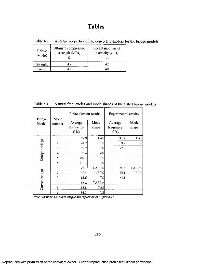
Tables
Table 4.1. Average properties o f the concrete cylinders for the bridge models
BridgeModel
Ultimate compressive strength (MPa)
fc
Secant modulus of elasticity (GPa)
EeStraight 45 42Curved 41 40
Table 5.1. Natural frequencies and mode shapes of the tested bridge models
BridgeModel
ModeFinite element results Experimental results
number AverageFrequency
(Hz)
Modeshape
Averagefrequency
(Hz)
Modeshape
1 29.9 L A P 31.2 L A PbO-o 2 44.7 L F 39.9 L FUh
3 72.7 T S 72.3-£3bO 4 75.4 T A S
5 102.3 L F
6 110.3 T S
bJO1 24.1 L A F - T S 24.5 L A F - T S
2 40.4 L F - T S 35.1 L F - T SVh 3 81.6 T S 64.1<U&3u
4 86.2 T A S - L F
5 88.8 T A S
6 98.3 T SN ote : Symbols fo r mode shapes are explained in Figure 6.11
216
Reproduced with permission of the copyright owner. Further reproduction prohibited without permission.
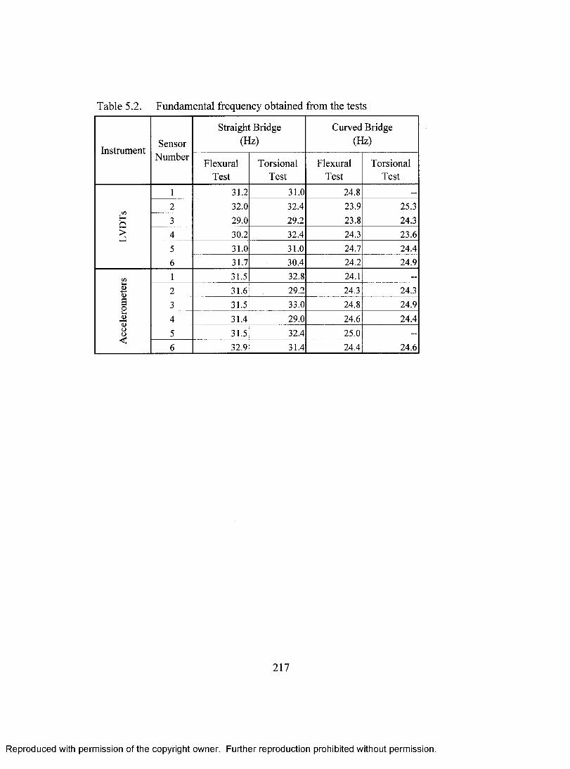
Table 5.2. Fundamental frequency obtained from the tests
Instrument SensorStraight Bridge
(Hz)Curved Bridge
(Hz)Number Flexural
TestTorsional
TestFlexural
TestTorsional
Test1 31.2 31.0 24.8 —
2 32.0 32.4 23.9 25.3HQ 3 29.0 29.2 23.8 24.3
4 30.2 32.4 24.3 23.65 31.0 31.0 24.7 24.46 31.7 30.4 24.2 24.9
1/3 1 31.5 32.8 24.1 —
(D 2 31.6 29.2 24.3 24.3So 3 31.5 33.0 24.8 24.9
1 3oo
4 31.4 29.0 24.6 24.45 31.5 32.4 25.0 —
< 3 6 32.9 31.4 24.4 24.6
217
Reproduced with permission of the copyright owner. Further reproduction prohibited without permission.

Table 6.1. Geometries o f bridges used in parametric study for load distribution factor
B r i d g e N u m b e r o f S p a n ( L ) N u m b e r o f K = C r o s s S e c t i o n D i m e n s i o n s ( m )l a n e s ( N l ) ( m ) b o x e s ( N b ) L / R A B C d H t i ta
( 1 ) ( 2 ) ( 3 ) ( 4 ) ( 5 ) ( 6 ) ( 7 ) ( 8 ) ( 9 ) ( 1 0 ) ( 1 1 ) ( 1 2 )2l-20-2b 2 0 2 9 .3 0 2 .3 2 5 0 .3 0 0 .8 0 1 .025 0 .0 1 6 0 .2 2 52l-20-3h 20 3 o 9 .3 0 1.550 0 .3 0 0 .8 0 1.025 0 .0 1 6 0 .2 2 52l-20-4h 2 0 4 2 9 .3 0 1.163 0 .3 0 0 .8 0 1 .025 0 .0 1 6 0 .2 2 52l-40-2b 40 2 9 .3 0 2 .3 2 5 0 .3 0 1.60 1 .825 0 .0 1 6 0 .2 2 52l-40-3b 40 3 o 9 .3 0 1 .550 0 .3 0 1.60 1 .8 2 5 0 .0 1 6 0 .2 2 52l-40-4b 40 4 9 .3 0 1.163 0 .3 0 1.60 1.825 0 .0 1 6 0 .2 2 52l-60-2b <U 60 2 9 .3 0 2 .3 2 5 0 .3 0 2 .4 0 2 .6 2 5 0 .0 1 6 0 .2 2 52l-60-3b 60 3 9 .3 0 1.550 0 .3 0 2 .4 0 2 .6 2 5 0 .0 1 6 0 .2 2 52l-60-4b (N 60 4 cs 9 .3 0 1.163 0 .3 0 2 .4 0 2 .6 2 5 0 .0 1 6 0 .2 2 52l-80-2h 80 2 oc 9 .3 0 2 .3 2 5 0 .3 0 3 .2 0 3 .4 2 5 0 .0 1 6 0 .2 2 52l-80-3b 80 3 o 9 .3 0 1 .550 0 .3 0 3 .2 0 3 .4 2 5 0 .0 1 6 0 .2 2 52l-80-4b 80 4 9 .3 0 1.163 0 .3 0 3 .2 0 3 .4 2 5 0 .0 1 6 0 .2 2 5
2l-100-2b 100 2 o" 9 .3 0 2 .3 2 5 0 .3 0 4 .0 0 4 .2 2 5 0 .0 1 6 0 .2 2 52l-100-3b 100 3 9 .3 0 1 .550 0 .30 4 .0 0 4 .2 2 5 0 .0 1 6 0 .2 2 52l-100-4b 100 4 9 .3 0 1.163 0 .3 0 4 .0 0 4 .2 2 5 0 .0 1 6 0 .2 2 53l-20-2b 2 0 2 13.05 3 .2 6 3 0 .3 0 0 .8 0 1.025 0 .0 1 6 0 .2 2 53l-20-3b 20 3 13.05 2 .1 7 5 0 .3 0 0 .8 0 1 .025 0 .0 1 6 0 .2 2 53l-20-4b 2 0 4 13.05 1.631 0 .3 0 0 .8 0 1.025 0 .0 1 6 0 .2 2 53l-20-5b 2 0 5 o 13 .05 1.305 0 .3 0 0 .8 0 1 .0 2 5 0 .0 1 6 0 .2 2 53l-20-6h 2 0 6 o 13.05 1 .088 0 .3 0 0 .8 0 1.025 0 .0 1 6 0 .2 2 53l-40-2b 40 2 13.05 3 .2 6 3 0 .3 0 1.60 1 .825 0 .0 1 6 0 .2 2 53l-40-3b 4 0 3 o 13 .05 2 .1 7 5 0 .3 0 1.60 1.825 0 .0 1 6 0 .2 2 53l-40-4b 40 4 13.05 1 .631 0 .3 0 1 .60 1 .825 0 .0 1 6 0 .2 2 53l-40-5b 4 0 5 13.05 1.305 0 .3 0 1.60 1.825 0 .0 1 6 0 .2 2 53l-40-6h 40 6 13.05 1 .088 0 .3 0 1 .60 1 .825 0 .0 1 6 0 .2 2 53l-60-2b 60 2 13 .05 3 .2 6 3 0 .3 0 2 .4 0 2 .6 2 5 0 .0 1 6 0 .2 2 53l-60-3b § 60 3 13.05 2 .1 7 5 0 .3 0 2 .4 0 2 .6 2 5 0 .0 1 6 0 .2 2 53l-60-4b S
hJ 60 4 13.05 1.631 0 .3 0 2 .4 0 2 .6 2 5 0 .0 1 6 0 .2 2 53l-60-5b 60 5 13.05 1.305 0 .3 0 2 .4 0 2 .6 2 5 0 .0 1 6 0 .2 2 53l-60-6b 60 6 13.05 1 .088 0 .3 0 2 .4 0 2 .6 2 5 0 .0 1 6 0 .2 2 53l-80-2b 80 2 13.05 3 .2 6 3 0 .3 0 3 .2 0 3 .4 2 5 0 .0 1 6 0 .2 2 53l-80-3b 80 3 OC 13.05 2 .1 7 5 0 .3 0 3 .2 0 3 .4 2 5 0 .0 1 6 0 .2 2 53l-80-4b 80 4 o 13 .05 1 .631 0 .3 0 3 .2 0 3 .4 2 5 0 .0 1 6 0 .2 2 53l-80-5b 80 5 13.05 1.305 0 .3 0 3 .2 0 3 .4 2 5 0 .0 1 6 0 .2 2 53l-80-6b 80 6 o ' 13.05 1 .088 0 .3 0 3 .2 0 3 .4 2 5 0 .0 1 6 0 .2 2 5
3l-100-2b 100 2 13.05 3 .2 6 3 0 .3 0 4 .0 0 4 .2 2 5 0 .0 1 6 0 .2 2 53l-100-3b 100 3 13.05 2 .1 7 5 0 .3 0 4 .0 0 4 .2 2 5 0 .0 1 6 0 .2 2 53l-100-4b 100 4 13.05 1.631 0 .3 0 4 .0 0 4 .2 2 5 0 .0 1 6 0 .2 2 53l-100-5b 100 5 13 .05 1 .305 0 .3 0 4 .0 0 4 .2 2 5 0 .0 1 6 0 .2 2 53l-100-6b 100 6 13 .05 1 .0 8 8 0 .3 0 4 .0 0 4 .2 2 5 0 .0 1 6 0 .2 2 54l-20-3b 20 3 16 .80 2 .8 0 0 0 .3 0 0 .8 0 1 .025 0 .0 1 6 0 .2 2 54l-20-4b 20 4 16 .80 2 .1 0 0 0 .3 0 0 .8 0 1.025 0 .0 1 6 0 .2 2 54l-20-5b 2 0 5 o 16 .80 1.680 0 .30 0 .8 0 1.025 0 .0 1 6 0 .2 2 54l-20-6b 20 6 CN 16 .80 1 .400 0 .3 0 0 .8 0 1 .025 0 .0 1 6 0 .2 2 54l-40-3h 4 0 3 16 .80 2 .8 0 0 0 .3 0 1.60 1.825 0 .0 1 6 0 .2 2 54l-40-4b 40 4 o 16 .80 2 .1 0 0 0 .3 0 1 .60 1.825 0 .0 1 6 0 .2 2 54l-40-Sb 40 5 16 .8 0 1 .6 8 0 0 .3 0 1 .60 1 .825 0 .0 1 6 0 .2 2 54l-40-6b 40 6 16 .80 1 .400 0 .3 0 1.60 1 .825 0 .0 1 6 0 .2 2 54l-60-3b 60 3 16 .80 2 .8 0 0 0 .3 0 2 .4 0 2 .6 2 5 0 .0 1 6 0 .2 2 54l-60-4b i 60 4 16 .80 2 .1 0 0 0 .3 0 2 .4 0 2 .6 2 5 0 .0 1 6 0 .2 2 54l-60-5b J 60 5 16 .80 1 .680 0 .3 0 2 .4 0 2 .6 2 5 0 .0 1 6 0 .2 2 54l-60-6b 60 6 cs 16 .80 1.400 0 .3 0 2 .4 0 2 .6 2 5 0 .0 1 6 0 .2 2 54l-80-3b 80 3 16 .80 2 .8 0 0 0 .3 0 3 .2 0 3 .4 2 5 0 .0 1 6 0 .2 2 54l-80-4b 80 4 00 16 .80 2 .1 0 0 0 .3 0 3 .2 0 3 .4 2 5 0 .0 1 6 0 .2 2 54l-80-Sh 80 5 16.80 1 .680 0 .30 3 .2 0 3 .4 2 5 0 .0 1 6 0 .2 2 54l-80-6b 80 6 o 16 .80 1 .400 0 .3 0 3 .2 0 3 .4 2 5 0 .0 1 6 0 .2 2 5
4l-l00-3b 100 3 o 16.80 2 .8 0 0 0 .3 0 4 .0 0 4 .2 2 5 0 .0 1 6 0 .2 2 54l-100-4h 100 4 16 .80 2 .1 0 0 0 .3 0 4 .0 0 4 .2 2 5 0 .0 1 6 0 .2 2 54l-100-5b 100 5 16 .80 1 .680 0 .3 0 4 .0 0 4 .2 2 5 0 .0 1 6 0 .2 2 54l-100-6b 100 6 16 .80 1 .400 0 .3 0 4 .0 0 4 .2 2 5 0 .0 1 6 0 .2 2 5
Note : Symbols fo r cross-sectional dimensions are explained in Figure 6.1
2 1 8
Reproduced with permission of the copyright owner. Further reproduction prohibited without permission.
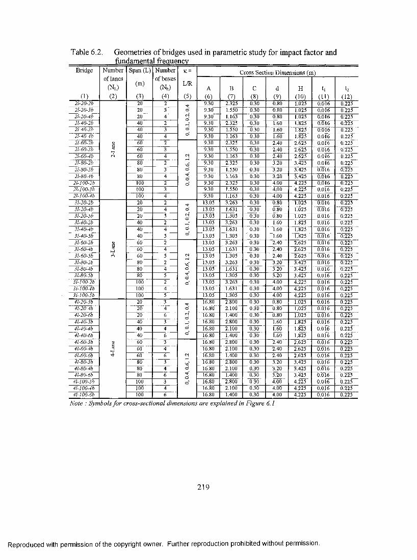
Table 6.2. Geometries o f bridges used in parametric study for impact factor and
B r i d g e N u m b e r S p a n ( L ) N u m b e r K = C r o s s S e c t i o n D i m e n s i o n s ( m )o t l a n e s
( N l )( m )
o f b o x e s( N b )
L / RA B C d H
0 ) ( 2 ) ( 3 ) ( 4 ) ( 5 ) ( 6 ) ( 7 ) ( 8 ) ( 9 ) ( 1 0 ) ( 1 1 ) ( 1 2 )2l-20-2b 20 2 9 .3 0 2 .3 2 5 0 .3 0 0 .8 0 1 .025 0 .0 1 6 0 .2 2 52l-20-3b 2 0 3 O 9 .3 0 1 .550 0 .3 0 0 .8 0 1 .025 0 .0 1 6 0 .2 2 52l-20-4b 20 4 CS 9 .3 0 1.163 0 .3 0 0 .8 0 1.025 0 .0 1 6 0 .2 2 52l-40-2b 40 2 9 .3 0 2 .3 2 5 0 .3 0 1.60 1 .8 2 5 0 .0 1 6 0 .2 2 52l-40-3b 40 3 9 .3 0 1 .550 0 .3 0 1 .60 1 .825 0 .0 1 6 0 .2 2 52l-40-4b 4 0 4 9 .3 0 1.163 0 .3 0 1.60 1.825 0 .0 1 6 0 .2 2 52l-60-2b § 60 2 9 .30 2 .3 2 5 0 .3 0 2 .4 0 2 .6 2 5 0 .0 1 6 0 .2 2 52l-60-3b 60 3 9 .3 0 1 .550 0 .3 0 2 .4 0 2 .6 2 5 0 .0 1 6 0 .2 2 52l-60-4b CS 60 4 cs 9 .3 0 1.163 0 .3 0 2 .4 0 2 .6 2 5 0 .0 1 6 0 .2 2 52l-80-2b 80 2 9 .3 0 2 .3 2 5 0 .3 0 3 .2 0 3 .4 2 5 0 .0 1 6 0 .2 2 52l-80-3b 80 3 o
d9 .3 0 1.550 0 .3 0 3 .2 0 3 .4 2 5 0 .0 1 6 0 .2 2 5
2l-80-4b 80 4 9 .3 0 1 .163 0 .3 0 3 .2 0 3 .4 2 5 0 .0 1 6 0 .2 2 52l-100-2b 100 2 o ' 9 .3 0 2 .3 2 5 0 .3 0 4 .0 0 4 .2 2 5 0 .0 1 6 0 .2 2 521-100-3b 100 3 9 .3 0 1.550 0 .3 0 4 .0 0 4 .2 2 5 0 .0 1 6 0 .2 2 52l-l00-4b 100 4 9 .3 0 1.163 0 .3 0 4 .0 0 4 .2 2 5 0 .0 1 6 0 .2 2 53l-20-2b 2 0 2 13 .05 3 .2 6 3 0 .3 0 0 .8 0 1 .025 0 .0 1 6 0 .2 2 53l-20-4b 20 4 o
cs13 .05 1.631 0 .3 0 0 .8 0 1 .025 0 .0 1 6 0 .2 2 5
3l-20-5b 2 0 5 13 .05 1.305 0 .3 0 0 .8 0 1.025 0 .0 1 6 0 .2 2 53l-40-2b 40 2 —r 13 .05 3 .2 6 3 0 .3 0 1.60 1.825 0 .0 1 6 0 .2 2 53l-40-4b 40 4 o
o13 .05 1.631 0 .3 0 1.60 1 .825 0 .0 1 6 0 .2 2 5
3l-40-5b 40 5 13 .05 1.305 0 .3 0 1.60 1 .825 0 .0 1 6 0 .2 2 53l-60-2b § 60 2 13 .05 3 .2 6 3 0 .3 0 2 .4 0 2 .6 2 5 0 .0 1 6 0 .2 2 53l-60-4b 5 60 4 13.05 1.631 0 .3 0 2 .4 0 2 .6 2 5 0 .0 1 6 0 .2 2 53 l6 0 -5 b CO 60 5 cs 13 .05 1.305 0 .3 0 2 .4 0 2 .6 2 5 0 .0 1 6 0 .2 2 53l-80-2b 80 2 d ' 13 .05 3 .2 6 3 0 .3 0 3 .2 0 3 .4 2 5 0 .0 1 6 0 .2 2 53l-80-4b 80 4 o 13.05 1.631 0 .3 0 3 .2 0 3 .4 2 5 0 .0 1 6 0 .2 2 53l-80-Sb 80 5 13.05 1.305 0 .3 0 3 .2 0 3 .4 2 5 0 .0 1 6 0 .2 2 5
3l-100-2b 100 2 o*' 13 .05 3 .2 6 3 0 .3 0 4 .0 0 4 .2 2 5 0 .0 1 6 0 .2 2 53l-100-4b 100 4 13.05 1.631 0 .3 0 4 .0 0 4 .2 2 5 0 .0 1 6 0 .2 2 53l-100-5b 100 5 13.05 1.305 0 .3 0 4 .0 0 4 .2 2 5 0 .0 1 6 0 .2 2 54l-20-3b 20 3 16 .80 2 .8 0 0 0 .3 0 0 .8 0 1 .025 0 .0 1 6 0 .2 2 54l-20-4b 20 4 o 16 .80 2 .1 0 0 0 .30 0 .8 0 1.025 0 .0 1 6 0 .2 2 54l-20-6b 20 6 16 .80 1 .400 0 .3 0 0 .8 0 1 .025 0 .0 1 6 0 .2 2 54 l40 -3b 40 3 16 .80 2 .8 0 0 0 .3 0 1.60 1 .825 0 .0 1 6 0 .2 2 54l-40-4b 40 4 o
o16 .80 2 .1 0 0 0 .3 0 1.60 1.825 0 .0 1 6 0 .2 2 5
4l-40-6h 40 6 16 .80 1.400 0 .3 0 1.60 1 .825 0 .0 1 6 0 .2 2 54l-60-3b 60 3 16 .80 2 .8 0 0 0 .3 0 2 .4 0 2 .6 2 5 0 .0 1 6 0 .2 2 54l-60-4b J 60 4 16 .80 2 .1 0 0 0 .3 0 2 .4 0 2 .6 2 5 0 .0 1 6 0 .2 2 54l-60-6b Tj- 60 6 cs 16.80 1.400 0 .3 0 2 .4 0 2 .6 2 5 0 .0 1 6 0 .2 2 54l-80-3b 80 3 d" 16 .80 2 .8 0 0 0 .3 0 3 .2 0 3 .4 2 5 0 .0 1 6 0 .2 2 54l-80-4b 80 4 o
d16 .80 2 .1 0 0 0 .3 0 3 .2 0 3 .4 2 5 0 .0 1 6 0 .2 2 5
4l-80-6b 80 6 16 .80 1.400 0 .3 0 3 .2 0 3 .4 2 5 0 .0 1 6 0 .2 2 54l-100-3b 100 3 o" 16 .80 2 .8 0 0 0 .3 0 4 .0 0 4 .2 2 5 0 .0 1 6 0 .2 2 54l-100-4b 100 4 16 .80 2 .1 0 0 0 .3 0 4 .0 0 4 .2 2 5 0 .0 1 6 0 .2 2 54l-W 0-6b 100 6 16.80 1.400 0 .3 0 4 .0 0 4 .2 2 5 0 .0 1 6 0 .2 2 5
N ote : Sym bols fo r cross-sectional dimensions are explained in Figure 6.1
219
Reproduced with permission of the copyright owner. Further reproduction prohibited without permission.

Table 6.3. Vehiclespeed used in parametric study for impact factoK =
L/R(1 )
Span length (L) (m)(2 )
Speed (v) (km/h)
(3)
0
20 12040 12060 12080 120too 120
0.120 98
40 120
0.220 70
40 98
0.4
20 5040 7060 8580 98
100 110
0.6
60 7080 80
100 90
1.2
60 5080 57
100 63
220
Reproduced with permission of the copyright owner. Further reproduction prohibited without permission.

Table 7.1. Comparison between the results obtained from the finite element analysis
M a x .S t r a i n i n g
D e a d L o a d A A S H T O1 9 9 6
A A S H T O L R F D 1 9 9 8
C H B D C2 0 0 0
A c t i o nF .E .M P r o p o s e d
m e th o d F .E .M P r o p o s e dm e t h o d F .E .M P r o p o s e d
m e t h o d F .E .M P r o p o s e dm e t h o d
a p ( M P a ) 4 6 5 3 2 0 2 2 3 6 4 4 4 2 4 5
a „ ( M P a ) 8 6 9 5 2 6 2 7 4 3 4 5 4 1 3 8
5 ( m ) 0 .0 3 4 0 .0 3 9 0 .0 1 6 0 .0 1 6 0 .0 2 8 0 .0 2 6 0 .0 3 4 0 .0 3 3
V ( k N ) 6 4 3 6 5 5 2 4 8 2 5 6 3 8 7 4 0 6 4 2 7 4 0 8
R e ( k N ) 6 0 2 6 4 6 2 2 0 2 5 5 3 6 7 4 0 5 4 2 5 4 8 8
R i ( k N ) 1 2 8 6 1 3 1 0 4 1 7 4 2 9 6 7 5 7 1 8 6 2 5 6 3 1
Rm ( k N ) 6 0 - 1 4 -8 3 - 8 0 - 1 3 9 - 1 2 8 - 1 7 2 - 1 5 4
221
Reproduced with permission of the copyright owner. Further reproduction prohibited without permission.
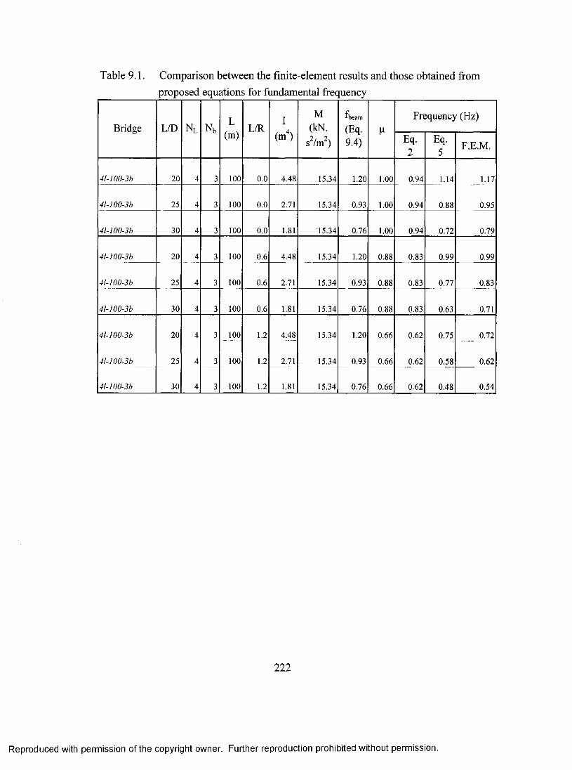
Table 9.1. Comparison between the fmite-element results and those obtained from proposed equations for fundamental frequency
Bridge L/D N l NbL
(m)L/R
I
(m'*)
M(kN.
s^/m^)
fbeam(Eq.9.4)
h
Frequency (Hz)
Eq.2
Eq.5
F.E.M.
4l-100-3b 2 0 4 3 too 0 .0 4 .4 8 1 5 .3 4 1 .2 0 1 .0 0 0 .9 4 1 .1 4 1 .1 7
4l-100-3b 2 5 4 3 too 0 .0 2 .7 1 1 5 .3 4 0 .9 3 1 .0 0 0 .9 4 0 .8 8 0 .9 5
4l-100-3b 3 0 4 3 too 0 .0 1 .8 1 1 5 .3 4 0 .7 6 1 .0 0 0 .9 4 0 .7 2 0 .7 9
41-100-3 b 2 0 4 3 too 0 .6 4 .4 8 1 5 .3 4 1 .2 0 0 .8 8 0 .8 3 0 .9 9 0 .9 9
4l-100-3b 2 5 4 3 too 0 .6 2 .7 1 1 5 .3 4 0 .9 3 0 .8 8 0 .8 3 0 .7 7 0 .8 3
4l-W0-3b 3 0 4 3 too 0 .6 1 .8 1 1 5 .3 4 0 .7 6 0 .8 8 0 .8 3 0 .6 3 0 .7 1
4l-I00-3b 2 0 4 3 too 1 .2 4 .4 8 1 5 .3 4 1 .2 0 0 .6 6 0 .6 2 0 .7 5 0 .7 2
4l-I00-3b 2 5 4 3 too 1 .2 2 .7 1 1 5 .3 4 0 .9 3 0 .6 6 0 .6 2 0 .5 8 0 .6 2
4l-100-3b 3 0 4 3 too 1 .2 1 .8 1 1 5 .3 4 0 .7 6 0 .6 6 0 .6 2 0 .4 8 0 .5 4
222
Reproduced with permission of the copyright owner. Further reproduction prohibited without permission.
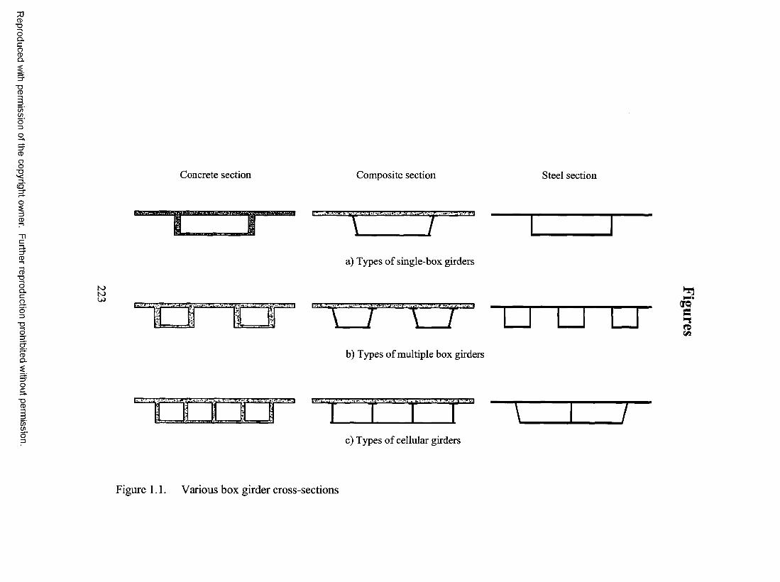
CD■DOQ.CoCDQ .
■DCD
(/)Wo'o
oo■oc 5 ‘
Concrete section Composite section Steel section
oCD
cCD
CD■oOQ .Cao= 5
1 7
N>K)
Da) Types of single-box girders
a O ' QTQS«n
CDa. b) Types of multiple box girders
oc■oCD
(/)o'= 3
I 7c) Types of cellular girders
Figure 1.1. Various box girder cross-sections
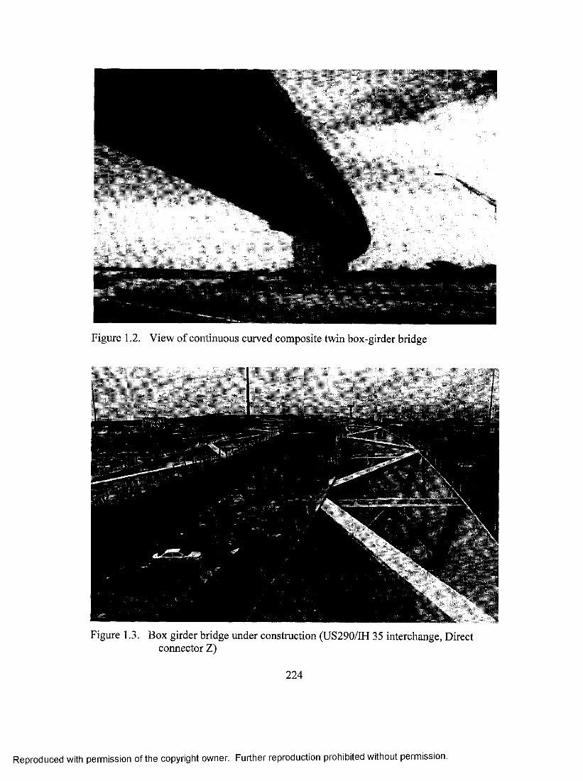
Figure 1.2. View of eontinuous curved composite twin box-girder bridge
Figure 1.3. Box girder bridge under construction (US290/IH 35 interchange, Direct connector Z)
224
Reproduced with permission of the copyright owner. Further reproduction prohibited without permission.
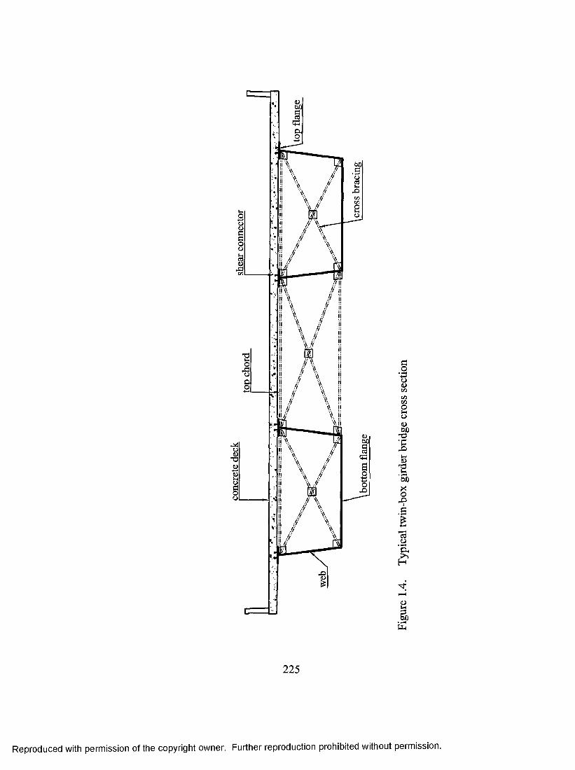
<D
§(UijiVit/1O)HoD00•cVhD•!a00X0
1
cSO‘BnH
(U
.1
225
Reproduced with permission of the copyright owner. Further reproduction prohibited without permission.
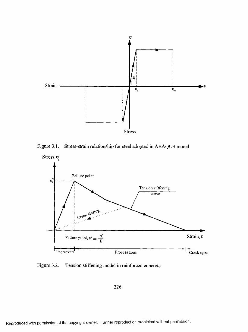
Strain
Stress
Figure 3.1. Stress-strain relationship for steel adopted in ABAQUS model
Stress, a
Failure point
Tension stiffeningcurve
Strain, sFailure point, s“ =
Uncracked Process zone Crack open
Figure 3.2. Tension stiffening model in reinforced concrete
226
Reproduced with permission of the copyright owner. Further reproduction prohibited without permission.
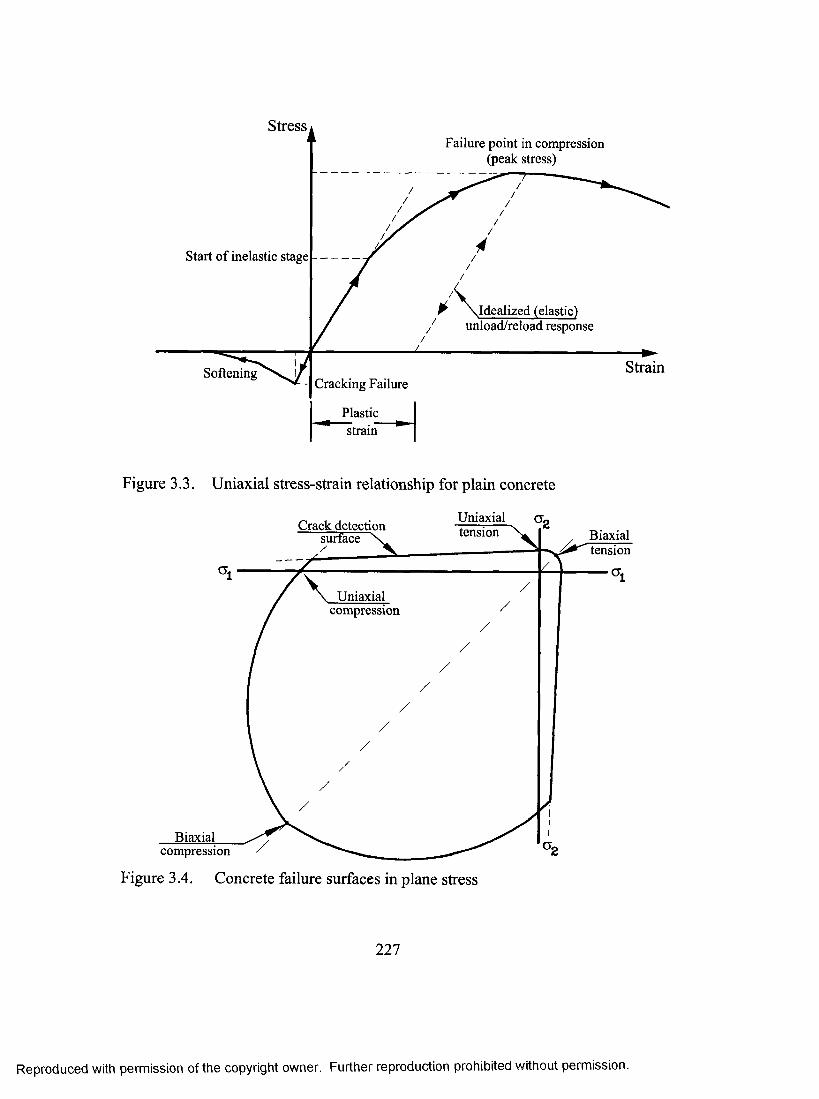
StressFailure point in compression
(peak stress)
Start of inelastic stage
\ldealized (elastic) unload/reload response
StrainSofteningCracking Failure
Plasticstrain
Figure 3.3. Uniaxial stress-strain relationship for plain concrete
UniaxialCrack detection surface \ tension Biaxial
tension
Uniaxialcompression
Biaxialcompression / _________
Figure 3.4. Concrete failure surfaces in plane stress
227
Reproduced with permission of the copyright owner. Further reproduction prohibited without permission.
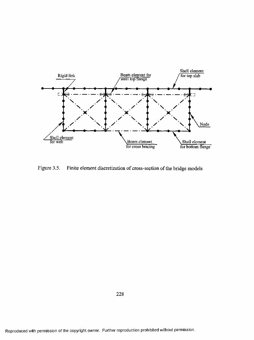
Shell elementBeam element for steel top tlange
Rigid link for top slab
Node
Shell elementBeam elementfor web Shell element
for cross bracing for bottom flange
Figure 3.5. Finite element discretization of cross-section of the bridge models
228
Reproduced with permission of the copyright owner. Further reproduction prohibited without permission.

SF2 SF3 SFlSF5 SF4
2(a) Output forces (c) Shell element "S4R"
(in ABAQUS)
SM2 SMISM3 SM3
2
1
(b) Output moments (d) REBAR in a shell
- Four-node element- Degrees of freedom- Output forces- Output moments- S t r e s s c o m p o n e n t s
U1,U2, U3,§l<l2,f3 SFl, SF2, SF3, SF4, SF5 SM1.SM2, SM3 811,822,512
- REBAR Option available in two directions
Figure 3.6. Shell element "S4R" used for plate modelling
229
Reproduced with permission of the copyright owner. Further reproduction prohibited without permission.

1 25•
(a) Integration points o f beam in space (for output results)
(b) Element "B31H" in ABAQUS
Two-node element Degrees of freedom Output forces Output moments Stress components
Ul, U2, U3,$l,$2,$3 SFl, SF2, SF3 SMI, SM2, SM3 S11,S12
Figure 3.7. Beam element "B3IH" for beam in space
230
Reproduced with permission of the copyright owner. Further reproduction prohibited without permission.
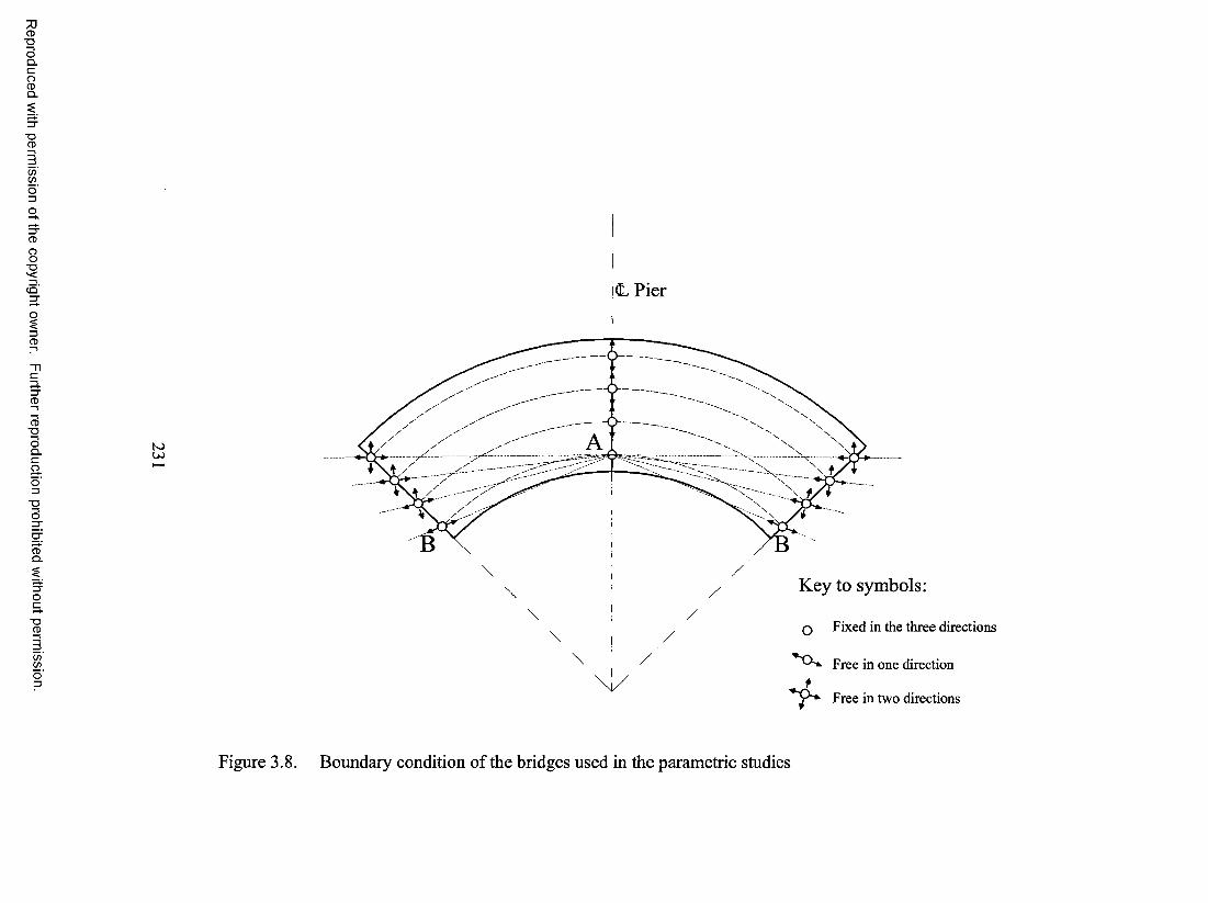
CD■DOQ .CoCDQ .
■DCD
C/)
o '3O
Oo■D
c5'
o3O"ncO’oCD
■DOQ .Caoo■Oo
CDQ .
■DCD
(/)(/)
tow
\ /Key to symbols
\O F i x e d i n t h e t h r e e d i r e c t i o n s
F r e e i n o n e d i r e c t i o n
F r e e i n t w o d i r e c t i o n s
Figure 3.8. Boundary condition of the bridges used in the parametric studies
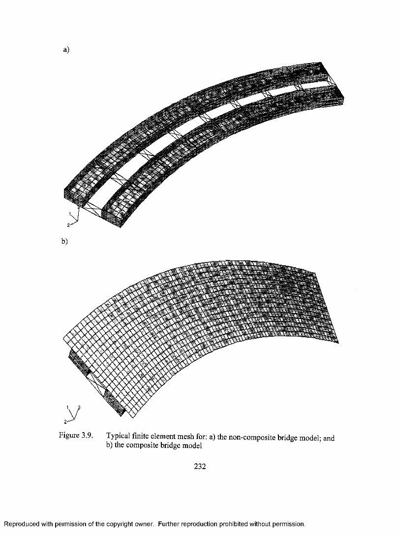
a)
b)
Figure 3.9. Typical finite element mesh for: a) the non-composite bridge model; and b) the composite bridge model
232
Reproduced with permission of the copyright owner. Further reproduction prohibited without permission.
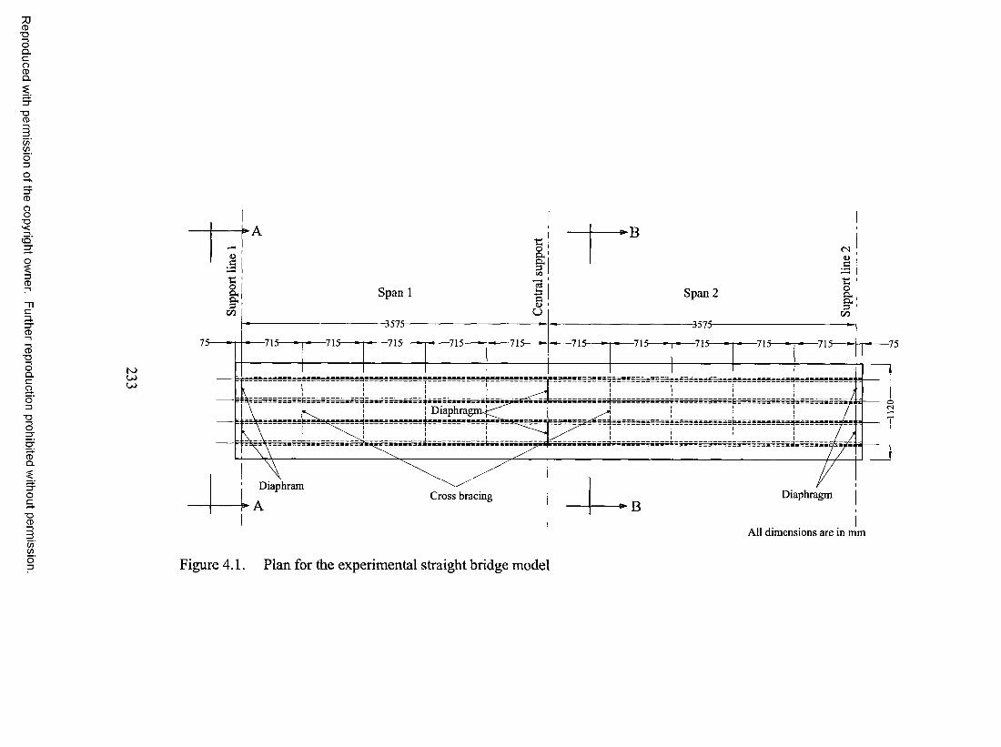
CD“DOQ.CoCDQ .
“DCD
C/)(/)
OO■D(5'
CD■aoQ .cao3T3O
CDQ .
■DCD
C/)C/)
toU)U)
&
Span 1 Span 2 &C/DO)
-3575- -3575
-715 -715 ■715 -715 -715 -715 -715 -715 -715
D ia p h r a g m .
D ia p h r a mD ia p h r a g mC r o s s b r a c in g
A l l d i m e n s i o n s a r e in m m
Figure 4.1. Plan for the experimental straight bridge model
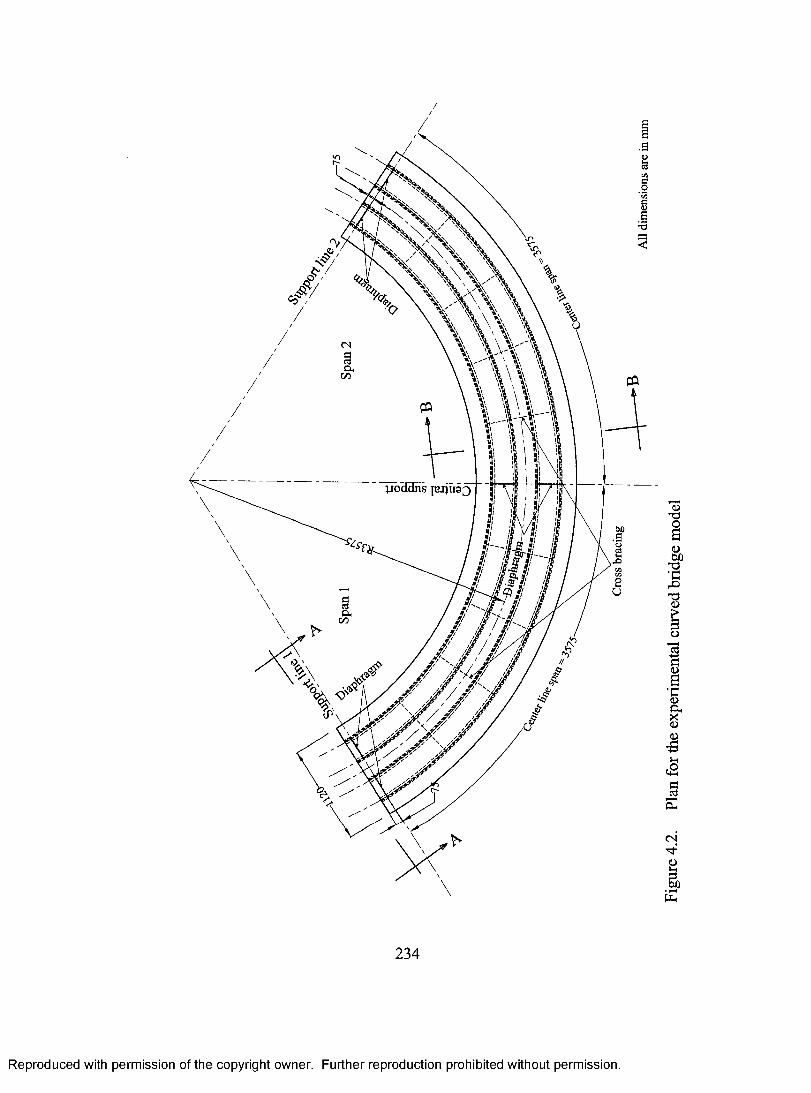
jjoddns
/<uo
(DbOT3•crOT30)
I(UB
•COhX!<u(U’B
)-(
sdcd
CN
U
P-l
234
Reproduced with permission of the copyright owner. Further reproduction prohibited without permission.
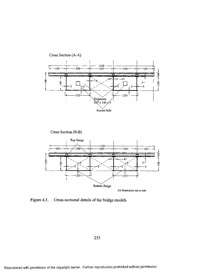
Cross Section (A-A)
1120-
-2 5 0 -•185- -250- ■250- 185-
O n O
-275- -275-l ia p h r a m
A c c e s s h o le
Cross Section (B-B)
T o p f la n g e
1120-
- 2 5 0 -•185- •250- -250- ■185-
3-1
■275- -275-
B o t t o m f la n g eA ll d im e n s io n s are in m m
Figure 4.3. Cross-sectional details o f the bridge models
235
Reproduced with permission of the copyright owner. Further reproduction prohibited without permission.

Figure 4.4. Tension test set-up for steel reinforcement specimen used in the bridge models
300
250
200Ph2
1<U2^ 100
0 ^ - - - - - - - - - - - - - - - - - - - - - - - i - - - - - - - - - - - - - - - - - - - - - - - - - 1- - - - - - - - - - - - - - - - - - - - - - - - - i - - - - - - - - - - - - - - - - - - - - - - - - - i----------- i---------- i-----------1----------- i-----------1----------0.000 0.002 0.004 0.006 0.008 0.010 0.012 0.014 0.016 0.018 0.020
T r u e s t r a in
Figure 4.5. True stress-true strain relationship for structural steel plate
236
Reproduced with permission of the copyright owner. Further reproduction prohibited without permission.
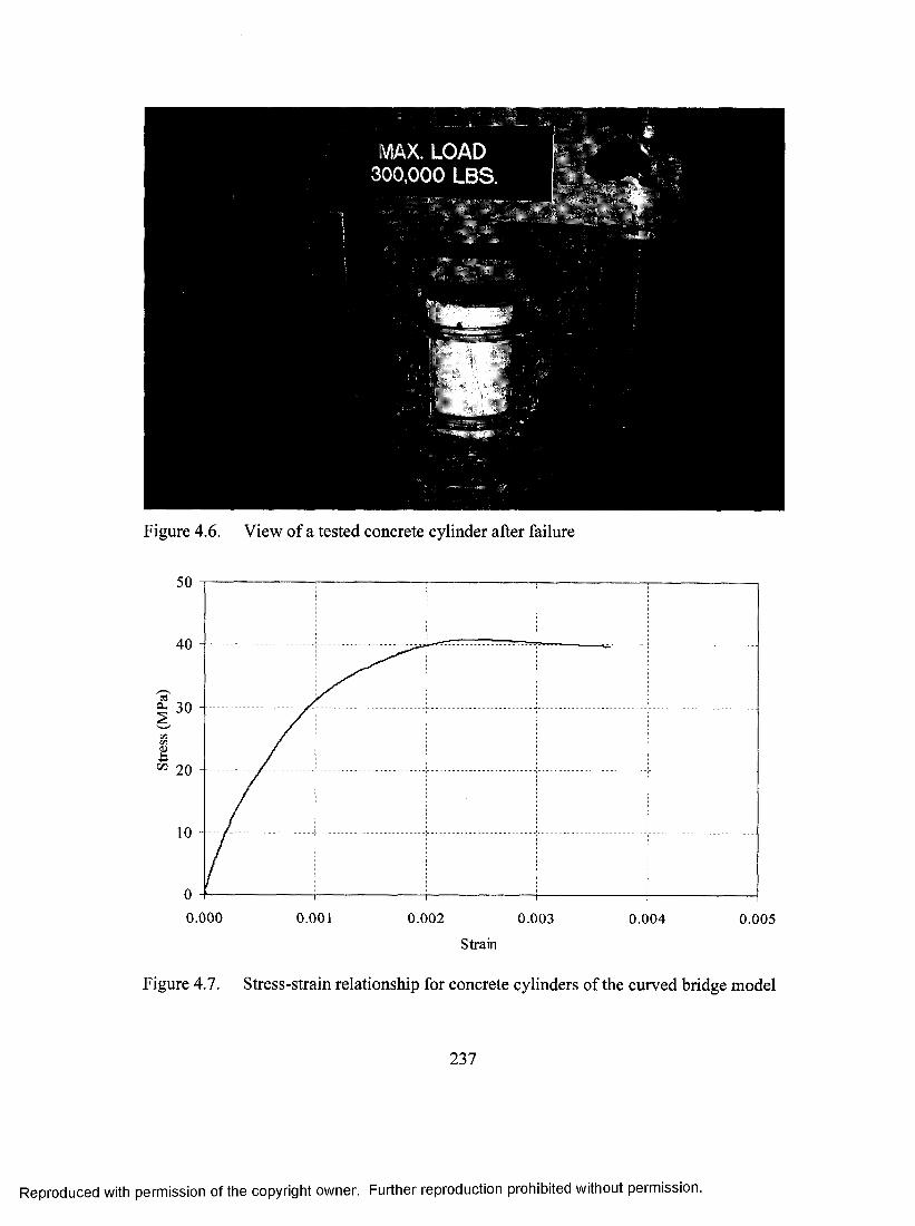
MAX. LOAD 300,000 LBS.
Figure 4.6. View of a tested concrete cylinder after failure
& 30
0.000 0.001 0.002 0.003 0.004 0.005Strain
Figure 4.7. Stress-strain relationship for concrete cylinders of the curved bridge model
237
Reproduced with permission of the copyright owner. Further reproduction prohibited without permission.

1000
8 0 0 -
S ' 6 0 0 -
200 -
0.000 0.002 0 .0 0 4 0 .0 0 6 0 .0 0 8 0.010 0.012 0 .0 1 4 0 .0 1 6 0 .0 1 8 0.020True Strain
Figure 4.8. Stress-strain relationship for the reinforcing steel
400
300 -
100 - <
0.000 0.002 0.004 0.006 0.008 0.010 0.012 0.014 0.016 0.018 0.020T r u e s tr a in
Figure 4.9. True stress-true strain relationship for steel shear eonnectors
238
Reproduced with permission of the copyright owner. Further reproduction prohibited without permission.
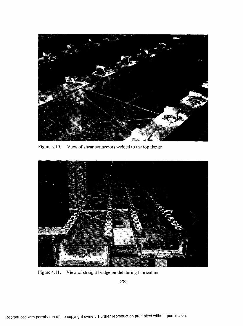
Figure 4.10. View of shear cormectors welded to the top flange
Figure 4.11. View of straight bridge model during fabrication
239
Reproduced with permission of the copyright owner. Further reproduction prohibited without permission.
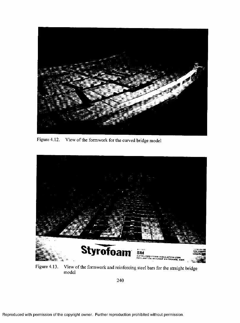
Figure 4.12. View of the formwork for the curved bridge model
Styrofoami m s u l a t i o n c o n
(SOLAWT DC MOUSSE
Figure 4.13. View of the formwork and reinforcing steel bars for the straight bridgemodel
240
Reproduced with permission of the copyright owner. Further reproduction prohibited without permission.
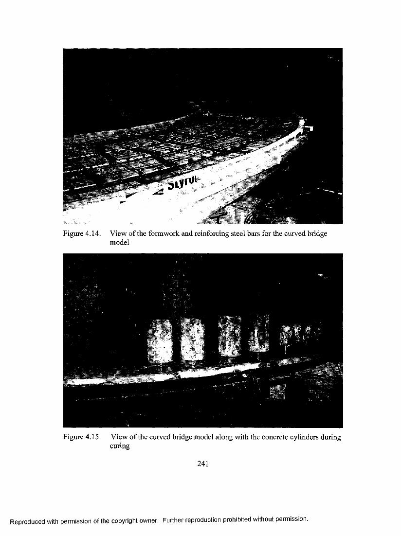
Figure 4.14. View of the formwork and reinforcing steel bars for the curved bridge model
Figure 4.15. View of the curved bridge model along with the concrete cylinders during curing
241
Reproduced with permission of the copyright owner. Further reproduction prohibited without permission.

Figure 4.16. View of the strain gauges installed along the bottom flange width at themid-span section
242
Reproduced with permission of the copyright owner. Further reproduction prohibited without permission.
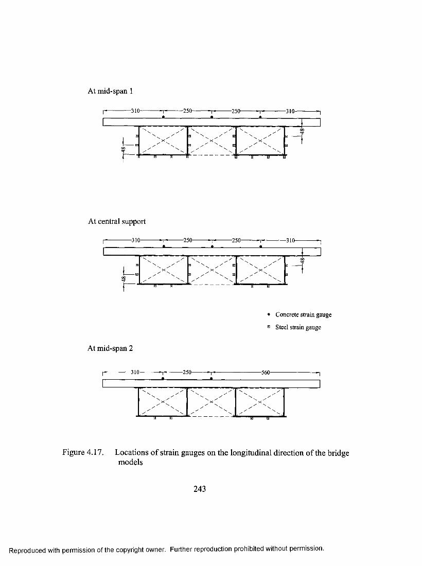
At mid-span 1
• A •. . 1
E
u .00Tl-1—
X^ X X ^
B------- S------ -
X X Xa ^ / E
Xa E
N ^ ^ /
X ^ X ^ X X
00
At central support
r -------------- 310— - 2 5 0 - - 2 5 0 n - - 3 1 0 -
X
At mid-span 2
• C o n c r e t e s tr a in g a u g e
® S t e e l s tr a in g a u g e
- 3 1 0 - - 2 5 0 - - 5 6 0 -
Figure 4.17. Locations o f strain gauges on the longitudinal direction of the bridge models
243
Reproduced with permission of the copyright owner. Further reproduction prohibited without permission.

Figure 4.18. View of the LYDTs in the first span of the bridge model
244
Reproduced with permission of the copyright owner. Further reproduction prohibited without permission.
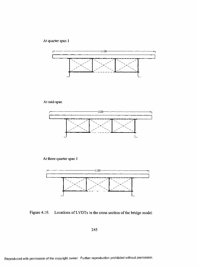
At quarter span 1
-1120-
At mid-span
- 1120 -
\ / •
\ /
X
At three-quarter span 1
- 1120-
Figure 4.19. Locations o f LVDTs in the cross section of the bridge model
245
Reproduced with permission of the copyright owner. Further reproduction prohibited without permission.

Figure 4.20. View of the accelerometers in the second span of the bridge model
246
Reproduced with permission of the copyright owner. Further reproduction prohibited without permission.

At quarter span 2
-1120-
/ V .
\ /
At mid-span 2
-1120-
■ "'1— ^ \ /
u
At three-quarter span 2
1120-
•N\
> c ^ ^ \ / ^ 'X
^ / \ / \^ 'N,
U 0
Figure 4.21. Locations o f accelerometers in the cross section of the bridge model
247
Reproduced with permission of the copyright owner. Further reproduction prohibited without permission.
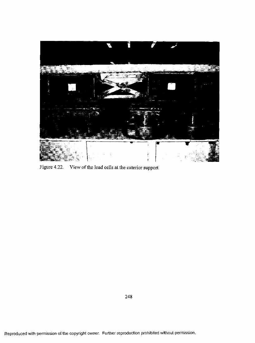
I
Figure 4.22. View of the load cells at the exterior support
248
Reproduced with permission of the copyright owner. Further reproduction prohibited without permission.
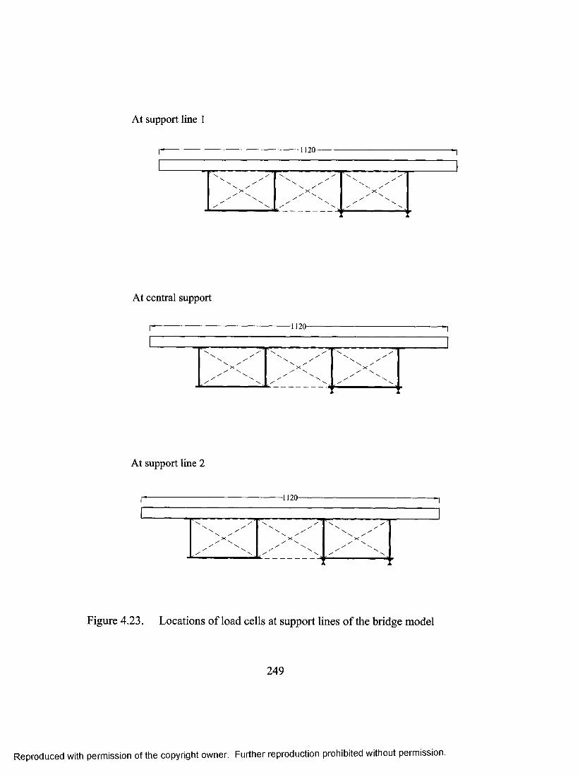
At support line 1
-1120-
At central support
- 1120 -
At support line 2
-1120-
Figure 4.23. Locations o f load cells at support lines of the bridge model
249
Reproducecl with permission of the copyright owner. Further reproduction prohibited without permission.
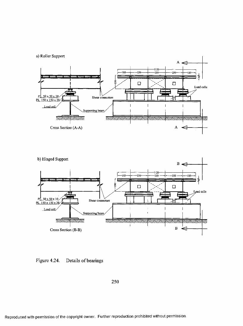
a) Roller Support
■1120--250-•185* ■250- -250- •185-----
Load cells
PL. 50 X 50 X 10/ PL. 150x 150x20.
Shear connectors
L o a d ce ll
Supporting beam.
C r o s s S e c t i o n ( A - A )
b) Hinged Support
1120--250--185- -250- -250^ -185— -
cells
PL. 50 X 50 X 10 PL. 150 X 150x20.
Shear connectors
Load cell.Supporting beam.
C r o s s S e c t i o n ( B - B )
Figure 4.24. Details o f bearings
250
Reproduced with permission of the copyright owner. Further reproduction prohibited without permission.
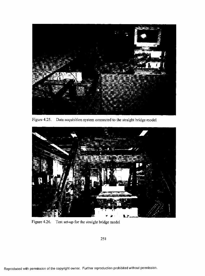
I
Figure 4.25. Data acquisition system connected to the straight bridge model
Figure 4.26. Test set-up for the straight bridge model
251
Reproduced with permission of the copyright owner. Further reproduction prohibited without permission.

Figure 4.27. View of Loading Case 1 applied to the non-composite straight bridgemodel
252
Reproduced with permission of the copyright owner. Further reproduction prohibited without permission.

Cast iron barLVDT
Jacking load downward
Figure 4.28. View of the flexural vibration test for straight bridge model
253
Reproduced with permission of the copyright owner. Further reproduction prohibited without permission.

Cast iron bar LVDT
Jacking load downward
Figure 4.29. View of the torsional vibration test for curved bridge model
254
Reproduced with permission of the copyright owner. Further reproduction prohibited without permission.

Figure 4.30. View of straight bridge model under Loading Case 1
Figure 4.31. View of straight bridge model imder Loading Case 2
255
Reproduced with permission of the copyright owner. Further reproduction prohibited without permission.
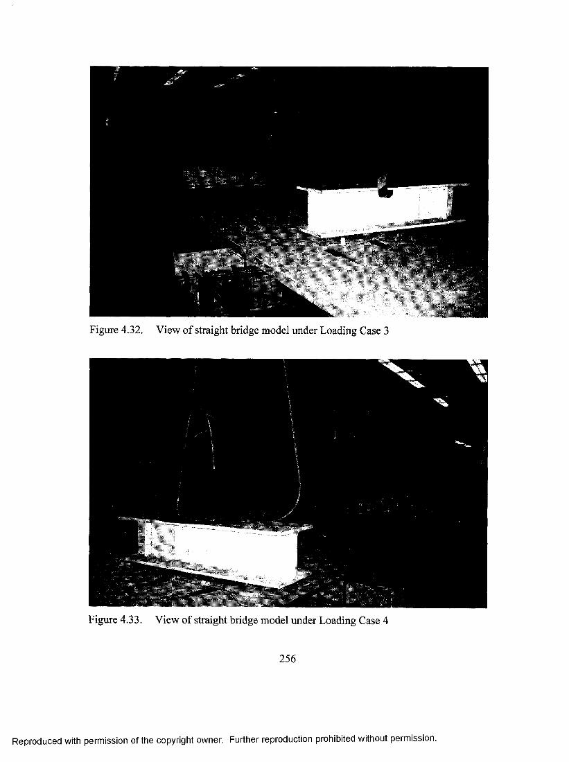
Figure 4.32. View of straight bridge model under Loading Case 3
Figure 4.33. View of straight bridge model under Loading Case 4
256
Reproduced with permission of the copyright owner. Further reproduction prohibited without permission.

Figure 4.34. View of curved bridge model under Loading Case 1
Figure 4.35. View of curved bridge model under Loading Case 2
257
Reproduced with permission of the copyright owner. Further reproduction prohibited without permission.
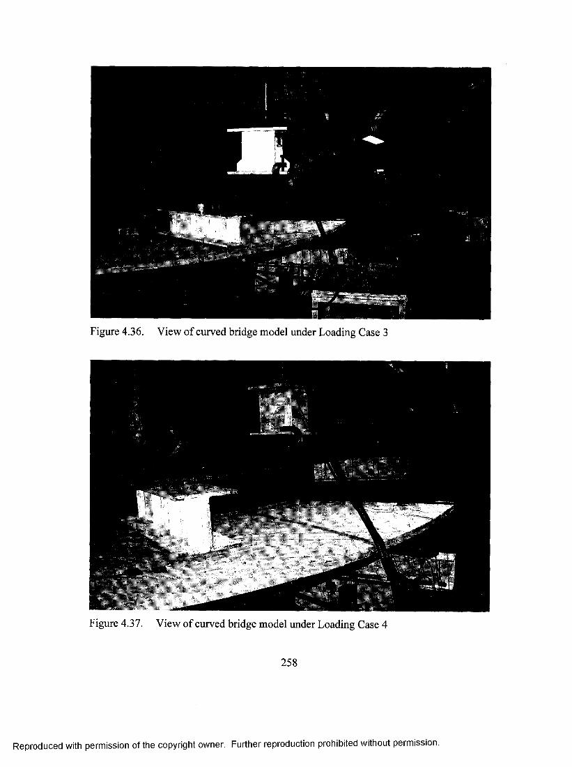
Figure 4.36. View of curved bridge model xmder Loading Case 3
Figure 4.37. View of curved bridge model under Loading Case 4
258
Reproduced with permission of the copyright owner. Further reproduction prohibited without permission.
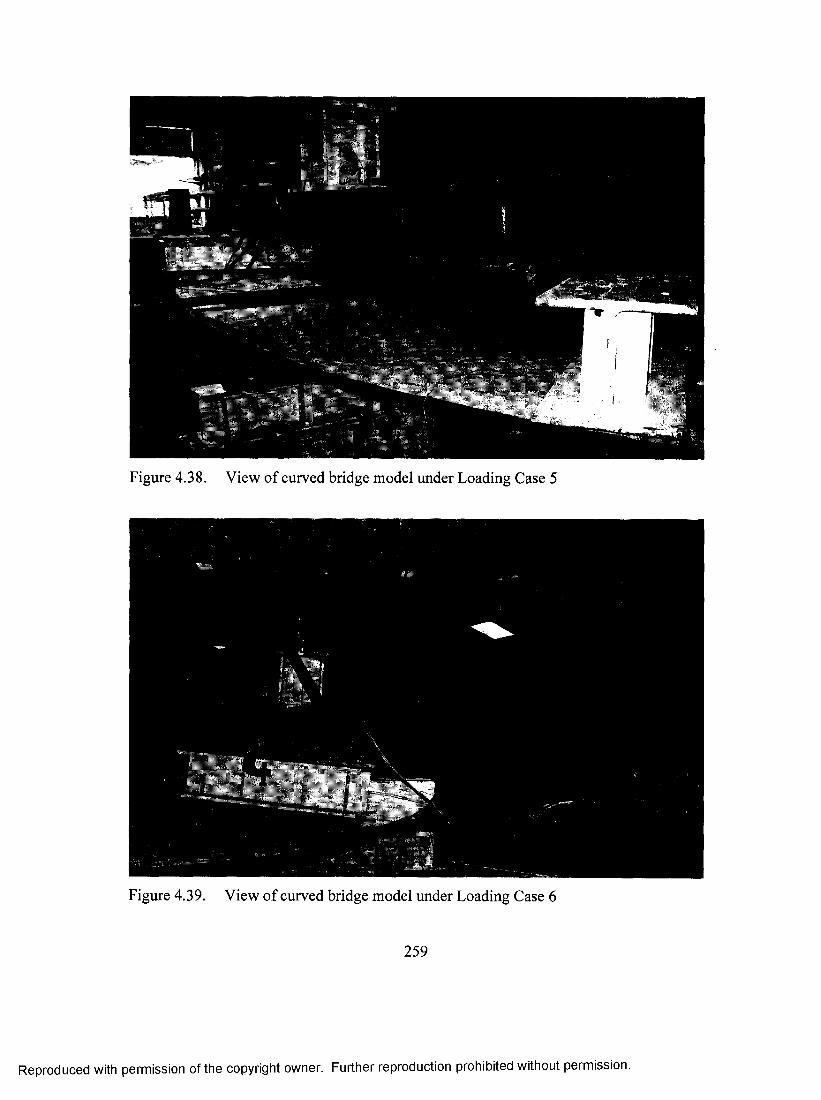
i
Figure 4.38. View of curved bridge model under Loading Case 5
Figure 4.39. View of curved bridge model under Loading Case 6
259
Reproduced with permission of the copyright owner. Further reproduction prohibited without permission.

a) Loading Case 15pan 1- 5pan 2 ~T-
S 14 B lo cks ; 14 Blocks!!^14 Blocl
!14 Blocks!
Cross Section
Planb) Loading Case 2
Blocks^ w 8 Blocks^ J 118 Blocks]
Cross Sectioni i i
Plan
c) Loading Case 3
^18 Blocks'V/ / / / / / / / / / / ,
K l8 Blocks; ! ! 1r 1 1 i 1
1 1 1 1 1 f i 1 1 1 1
r . i __ IC ro ss S e c tio n
d) Loading Case 4Plan
V777777777, 18 Blocks /
Vr/%
Cross Section
e) Loading Case 5W77777777m / 1 8 B locksV '/ // / // / / / / /
Cross Section
^ V ///M /////X n Blocks
" " 4 .1 ----- 1 - - - - - - - 1 - - - - - - - 1 -- - - - - - J- - - - - - - - -
Plan
Figure 5.1. Cases of loading for non-composite straight bridge model
260
Reproduced with permission of the copyright owner. Further reproduction prohibited without permission.

0.0 0.00.0 0.0
(a) Deflections at L/4 from the outer support in span (1)
0.0 0.00.0 0.0
(b) Deflections at mid span (1) F i n i t e - e l e m e n t r e s u lt s
• E x p e r im e n t a l r e su lts
V a lu e s a r e in m il l im e te r s
0.0 0.00.0 0.0
(c) Deflections at 3L/4 from the outer support in span (1)
Figure 5.2. Deflections of the non-composite straight bridge model due to Loading Case 1
261
Reproduced with permission of the copyright owner. Further reproduction prohibited without permission.
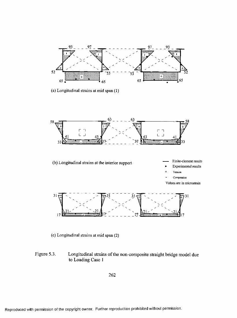
52 ~5J
65
(a) Longitudinal strains at mid span (1)
(b) Longitudinal strains at the interior support — F i n i t e - e l e m e n t re su lts • E x p e r im e n t a l r e s u lt s+ Tension
Compression
V a lu e s a r e in m ie r o s tr a in
31'
17
31 3L
17' \ 2 U ' _ " ^2\J.
r31
17
(c) Longitudinal strains at mid span (2)
Figure 5.3. Longitudinal strains o f the non-composite straight bridge model due to Loading Case 1
262
Reproduced with permission of the copyright owner. Further reproduction prohibited without permission.

CO■ooQ .coCDQ .
■oCD
C/)
o'o
oo■ov<cq' S u p p o r t l i n e 1 C e n t r a l s u p p o r t S u p p o r t l i n e 2
oCD
Cp.
CD■oOQ .Cao3■oo
Finite-elementresults
o o o
to
Values are in kN
CDQ .
O’o■DCD
Experimentalresults
C/)(/)Figure 5.4. Reactions for the non-composite straight bridge model due to Loading Case 1
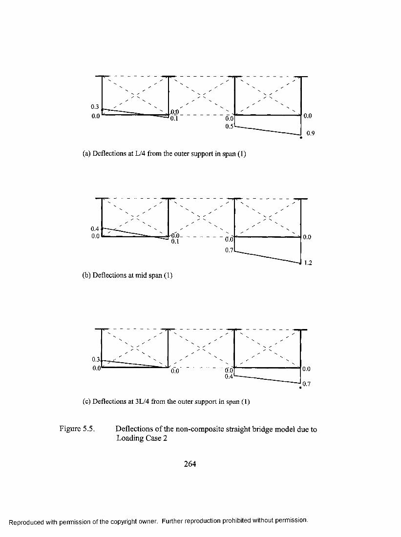
0.30.0 0.00.0
0.50.9
(a) Deflections at L/4 from the outer support in span (1)
0.40.0 0.0
0.7
(b) Deflections at mid span (1)
0.00.4
0.0
0.7
(c) Deflections at 3L/4 from the outer support in span (1)
Figure 5.5. Deflections of the non-composite straight bridge model due to Loading Case 2
264
Reproduced with permission of the copyright owner. Further reproduction prohibited without permission.
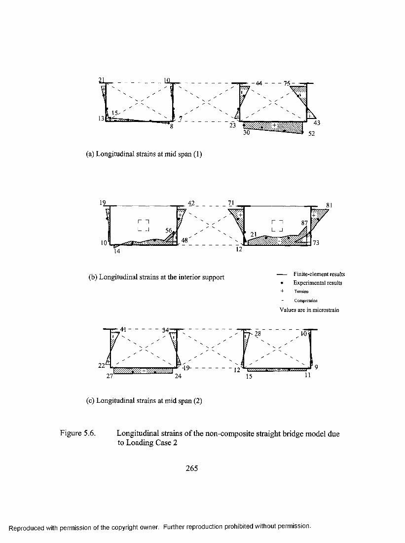
-4 4 -------- 7 5 -
(a) Longitudinal strains at mid span (1)
(b) Longitudinal strains at the interior support
22
34:
k.49-27 247 :
(c) Longitudinal strains at mid span (2)
12
rr2 8
F i n i t e - e l e m e n t r e s u lt s• E x p e r im e n t a l r e su lts+ Tension
Compression
V a lu e s a r e in m ic r o s tr a in
15
M)
11
Figure 5.6. Longitudinal strains o f the non-composite straight bridge model due to Loading Case 2
265
Reproduced with permission of the copyright owner. Further reproduction prohibited without permission.
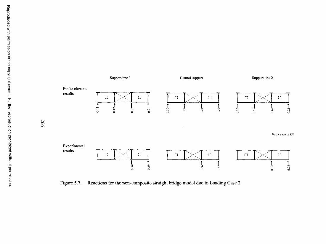
CD■DOQ .CoCDQ .
■DCD
C/)(/)
OO■D<5‘ Support line 1 Central support Support line 2
3.
CD■DOQ .Cao■oo
Finite-elementresults
o (No
toOsOs
Values are in kN
CDQ .
■DCD
Experimentalresults
C/)C/)
Figure 5.7. Reactions for the non-composite straight bridge model due to Loading Case 2
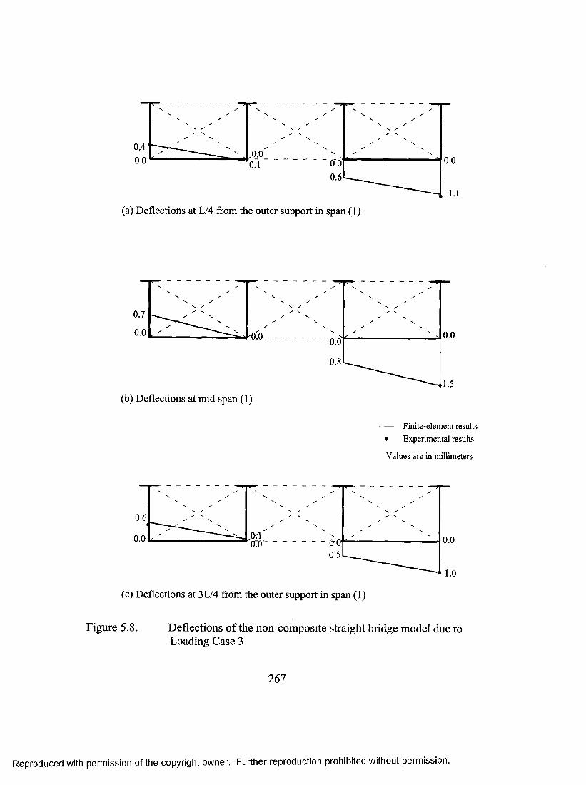
0.40.0 0.00.0
0.6
(a) Deflections at L/4 from the outer support in span (1)
0.7
0.0 0.0
(b) Deflections at mid span (1)
— F i n i t e - e l e m e n t r e s u lt s • E x p e r im e n t a l r e s u lt s
V a lu e s a r e in m il l im e te r s
0.6
0.0 0.0e-.o0.5
(c) Deflections at 3L/4 from the outer support in span (1)
Figure 5.8. Deflections o f the non-composite straight bridge model due to Loading Case 3
267
Reproduced with permission of the copyright owner. Further reproduction prohibited without permission.

37
(a) Longitudinal strains at mid span (1)
54
I------1
(b) Longitudinal strains at the interior support F in i t e - e l e m e n t r e s u lt s• E x p e r im e n t a l r e s u lt s+ Tension
Compression
V a lu e s a r e in m ic r o s tr a in
(c) Longitudinal strains at mid span (2)
37
Figure 5.9. Longitudinal strains o f the non-composite straight bridge model due to Loading Case 3
268
Reproduced with permission of the copyright owner. Further reproduction prohibited without permission.

73CD■DOQ .CoCDQ .
"DCD
(/)C/)
CD
OO■DS u p p o r t l i n e 1 C e n t r a l s u p p o r t S u p p o r t l i n e 2
CD
CD■DOQ .Cao
■oo
CDQ .
■DCD
Finite-elementresults
toa'O
Values are in kN
Experimentalresults
C/)if)Figure 5.10. Reactions for the non-composite straight bridge model due to Loading Case 3
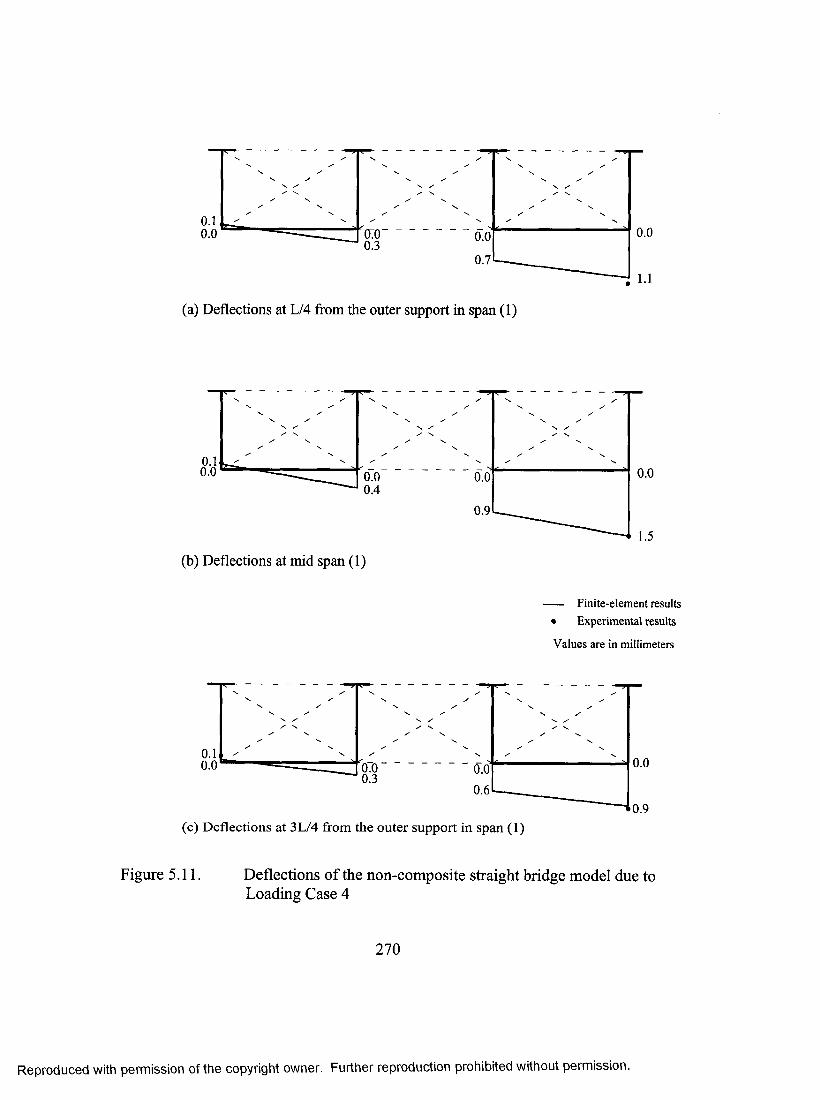
"o:o0.3
0.00.0 0.00.7
(a) Deflections at L/4 from the outer support in span (1)
0.0 0.00.00.4
0.0
0.9
(b) Deflections at mid span (1)
— F i n i t e - e l e m e n t r e su lts • E x p e r im e n t a l r e s u lt s
V a lu e s a r e in m il l im e te r s
0.00.0 0700.3
0.00.6
(c) Deflections at 3 L/4 from the outer support in span (1)
Figure 5.11. Deflections of the non-composite straight bridge model due to Loading Case 4
270
Reproduced with permission of the copyright owner. Further reproduction prohibited without permission.

-57
(a) Longitudinal strains at mid span (1)
50
32
58
(b) Longitudinal strains at the interior support F i n i t e - e l e m e n t r e s u lt s• E x p e r im e n t a l r e s u lt s+ Tension
Compression
V a lu e s a r e in m ic r o s tr a in
10 IS
11 Ij\ 14" •'I
29
13
(c) Longitudinal strains at mid span (2)
Figure 5.12. Longitudinal strains of the non-composite straight bridge model due to Loading Case 4
271
Reproduced with permission of the copyright owner. Further reproduction prohibited without permission.

7JCD■DOQ .CoCDQ .
■DCD
(/)(/)
CD
OO■DS u p p o r t l i n e 1 C e n tr a l s u p p o r t S u p p o r t l i n e 2
CD■DOQ .C9-o■oo
Finite-elementresults
to-oto
Values are in kN
CDQ .
■aCD
Experimentalresults
(/)(/)Figure 5.13. Reactions for the non-composite straight bridge model due to Loading Case 4

0.00.5
0.0'0.5
0.00.5
0.00.5
(a) Deflections at L/4 from the outer support in span (1)
0.0
0.60.0
0.7
0.0
0.7
0.0
0.6
(b) Deflections at mid span (1)
— F i n i t e - e l e m e n t r e s u lt s • E x p e r im e n t a l r e su lts
V a lu e s a r e in m il l im e te r s
0.00.4.
0.00.4
0,00.4
0.00.4
(c) Deflections at 3L/4 from the outer support in span (1)
Figure 5.14. Deflections o f the non-composite straight bridge model due to Loading Case 5
273
Reproduced with permission of the copyright owner. Further reproduction prohibited without permission.
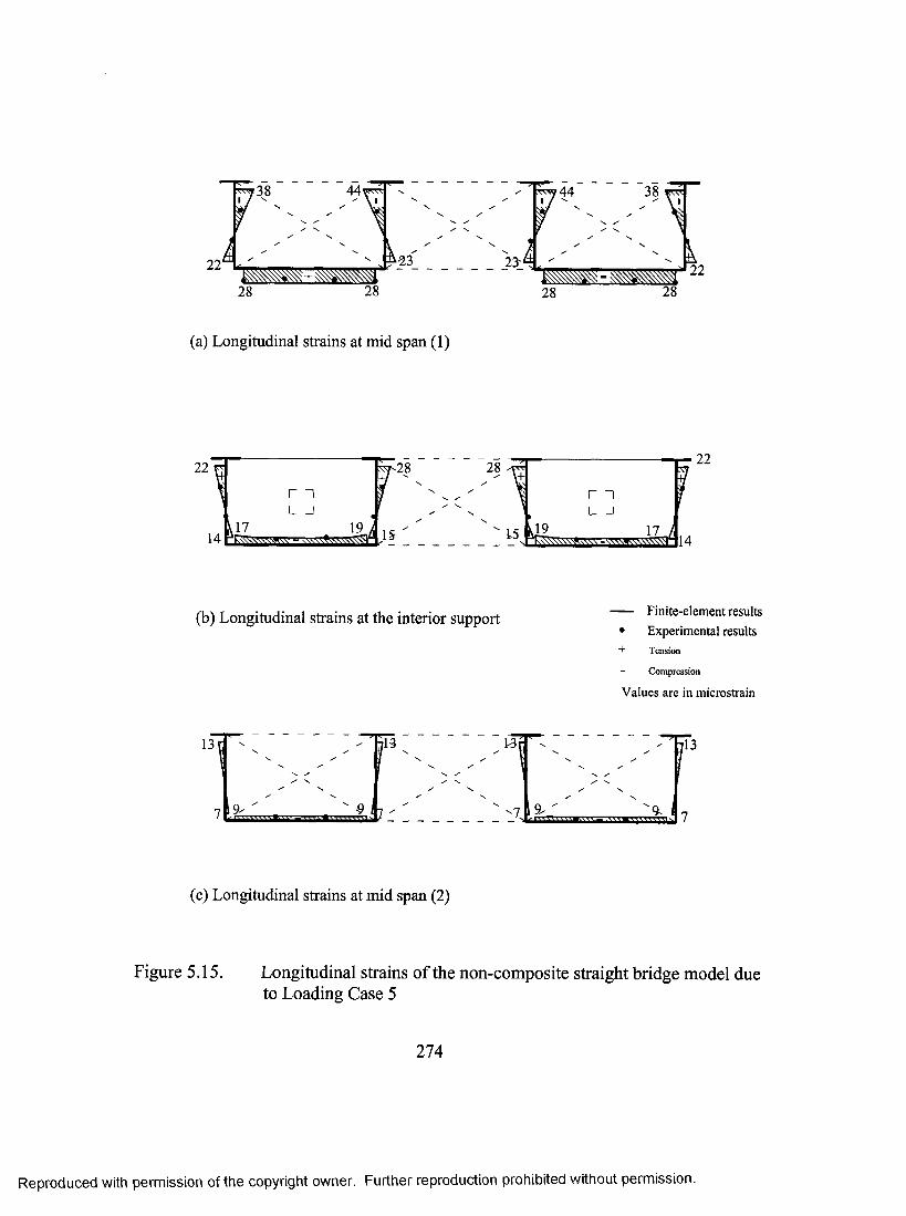
22i
f 38 4 4 ^\ I
k23
28 28
23-i
^ 4 4I / '' 38
28
k22
28
(a) Longitudinal strains at mid span (I)
22 28I 1I I
17 \9 A I S
28
15
I - - - - - - - - - - 1
I_ _ _ _ _ _ I
22
IK19 17 H14
(b) Longitudinal strains at the interior support — F i n i t e - e l e m e n t r e s u lt s • E x p e r im e n t a l r e su lts+ Tension
Compression
V a lu e s a r e in m ic r o s tr a in
13 fl3r
(c) Longitudinal strains at mid span (2)
Figure 5.15. Longitudinal strains of the non-composite straight bridge model due to Loading Case 5
274
Reproduced with permission of the copyright owner. Further reproduction prohibited without permission.
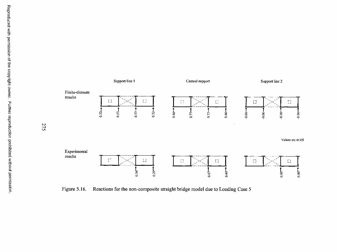
7JCD-oOQ .coCDQ .
■oCD
I(/)o'oo
oo■oc q ' S u p p o r t l i n e 1 C e n t r a l s u p p o r t S u p p o r t l i n e 2
QCD
Cp.O’oCD■aoQ .cao3■Oo
Finite-elementresults
oK>LTi
Values are in kN
CDQ .
O’oc■oCD
Experimentalresults
C/)C/)Figure 5.16. Reactions for the non-composite straight bridge model due to Loading Case 5

a) Loading Case 1
^ 1 4 Blocks^ / / / / / / / / / . ^14 Blocks''^///////////. V,\A Blocks:
Cross Section
b) Loading Case 2
14 B l o c k s k l 4 Blocksy /y /^ /y /A \/yy/yyy/y.
Cross Section
c) Loading Case 3
Kl4 Blocks; ;14 Blocks ///////////
Cross Section
d) Loading Case 4
p l4 Blockss3'^r
Cross Section
e) Loading Case 57777777777/ 'A A Blocks/
'yyyy/yyyyyy. <ICross Section
Plan
Figure 5.17. Cases of loading for the non-composite curved bridge model
276
Reproduced with permission of the copyright owner. Further reproduction prohibited without permission.
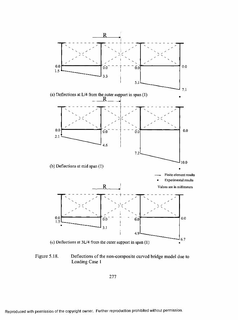
0.0 0.00.0 0.0
3.3
(a) Deflections at L/4 from the outer support in span (1)
0.0 0.00.0 0.0
4.6
7.2
10.0(b) Deflections at mid span (1)
F i n i t e - e l e m e n t r e su lts• E x p e r im e n t a l r e s u lt s
V a lu e s a r e in m il l im e te r s
0.0 0.00.0 0.0
4.96.7
(c) Deflections at 3L/4 from the outer support in span (1)
Figure 5.18. Deflections of the non-composite curved bridge model due to Loading Case 1
277
Reproduced with permission of the copyright owner. Further reproduction prohibited without permission.

R
50
39 J4-■38
(a) Longitudinal strains at mid span (1)
114
120’
151
205;116
168 150
123K(b) Longitudinal strains at the interior support F i n i t e - e l e m e n t r e s u lt s
E x p e r im e n t a l r e s u lt s+ Tension
Compression
V a lu e s a r e in m ic r o s tr a in
-73- - -92 116
(c) Longitudinal strains at mid span (2)
Figure 5.19. Longitudinal strains o f the non-composite curved bridge model due to Loading Case 1
278
Reproduced with permission of the copyright owner. Further reproduction prohibited without permission.
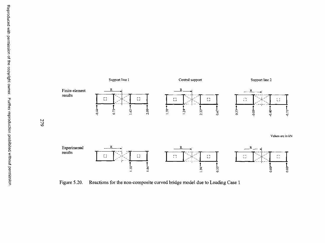
7]CD■oOQ .CoCDQ .
■oCD
C/)
o'13
OoT 3v<c q ' S u p p o r t l i n e I C e n t r a l s u p p o r t S u p p o r t l i n e 2
QCD
Cp.
CD■oOQ .CaoQ■oo
Finite-elementresults
<srs o
to<1
Values are in kN
CDQ .
Oc■oCD
Experimentalresults
(/>o'Q Figure 5.20. Reactions for the non-composite curved bridge model due to Loading Case 1
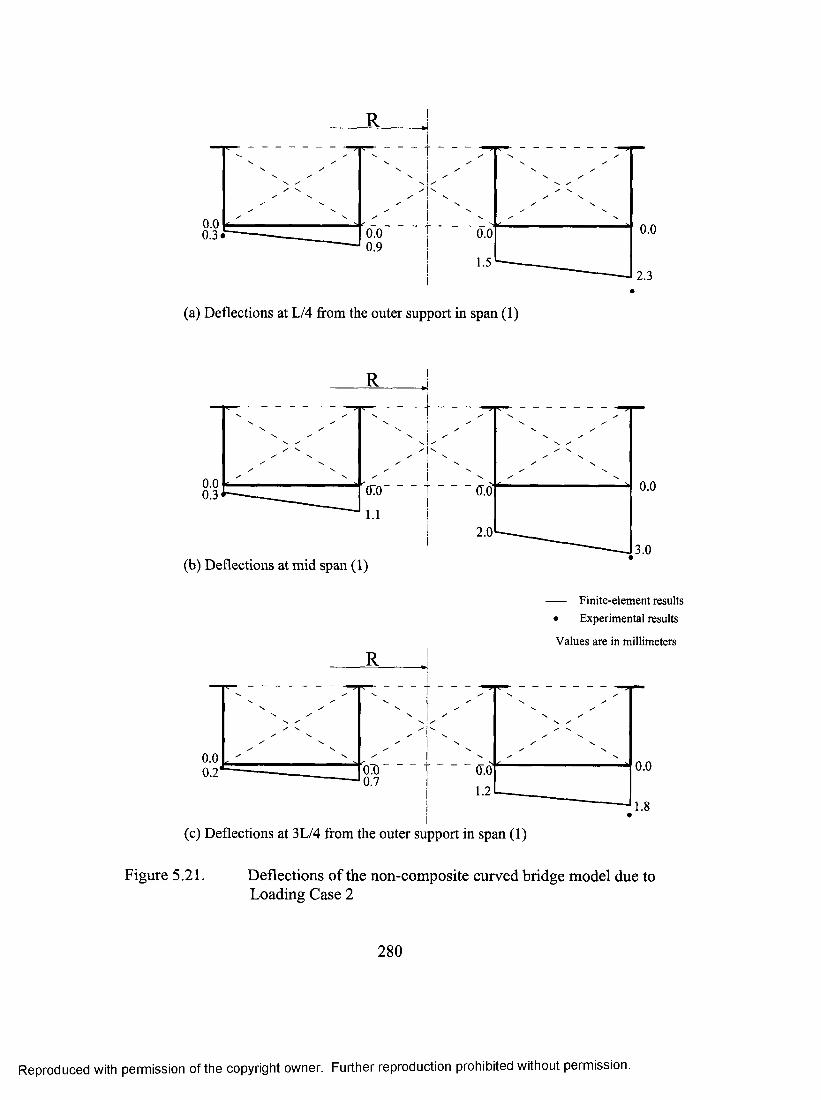
0.00.3. 0.00.0
0.90.0
2.3
(a) Deflections at L/4 from the outer support in span (1)
R
0.00.3 (TO'
1.1
(b) Deflections at mid span (1)
0.0
2.03.0
— F in i t e - e l e m e n t r e s u lt s • E x p e r im e n t a l r e su lts
V a lu e s a r e in m il l im e te r sR
0.00 .2* 0.0
0.70.0
(c) Deflections at 3 L/4 from the outer support in span (1)
Figure 5.21. Deflections of the non-composite curved bridge model due toLoading Case 2
280
Reproduced with permission of the copyright owner. Further reproduction prohibited without permission.
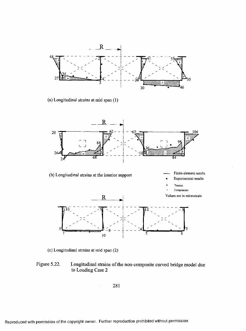
R
- - 20 -
^ 4 1I / ^
30
^35
'46
(a) Longitudinal strains at mid span (1)
104
I _ _ _ _ _ _ 1
(b) Longitudinal strains at the interior support
R
33
- 8- -
10
F i n i t e - e l e m e n t r e s u lt s• E x p e r im e n t a l r e s u lt s+ Tension
Compression
V a lu e s a r e in m ic r o s tr a in
(c) Longitudinal strains at mid span (2)
Figure 5.22. Longitudinal strains of the non-composite curved bridge model due to Loading Case 2
281
Reproduced with permission of the copyright owner. Further reproduction prohibited without permission.
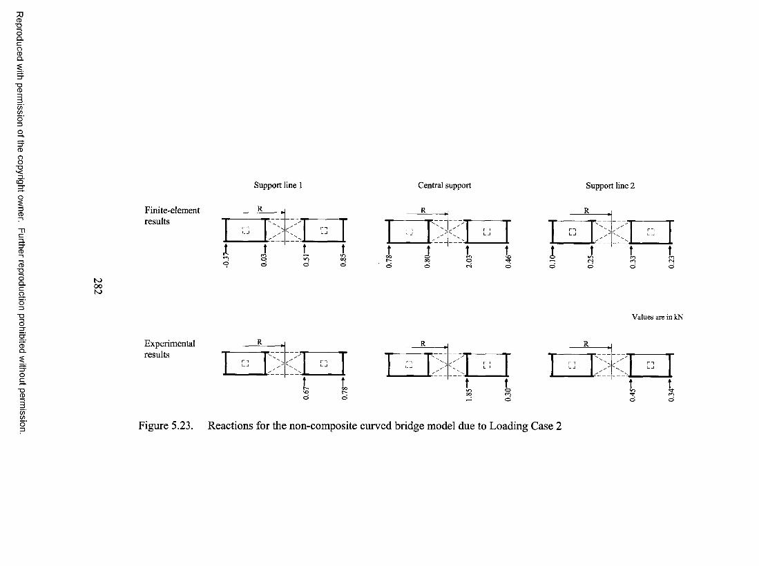
CD■DOQ.CoCDQ .
■DCD
C/)(/)
OO■Dc q ' S u p p o r t l i n e 1 C e n t r a l s u p p o r t S u p p o r t l i n e 2
O’QCD■DOQ .Cao■oo
Finite-elementresults
R R
oo o oto00to
Values are in kN
CDQ .
"DCD
Experimentalresults
R R
O O(/)(/)
Figure 5.23. Reactions for the non-composite curved bridge model due to Loading Case 2
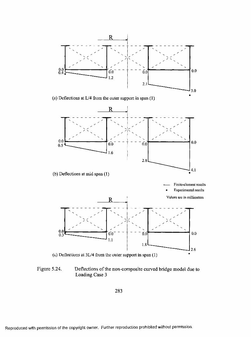
R
0.00 .4 , 0.0
1.2
0.00.0
3.0
(a) Deflections at L/4 from the outer support in span (1)
0.00.5
0.00.0 0.0
(b) Deflections at mid span (1)
F i n i t e - e l e m e n t r e s u lt s• E x p e r im e n t a l r e su lts
V a l u e s a r e in m il l im e te r s
0.00.3 0.00.0 O.tf
2.6(c) Deflections at 3L/4 from the outer support in span (1)
Figure 5.24. Deflections of the non-composite curved bridge model due to Loading Case 3
283
Reproduced with permission of the copyright owner. Further reproduction prohibited without permission.
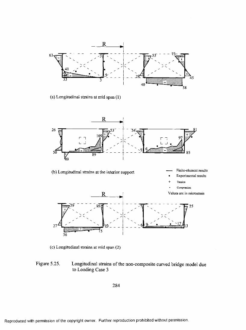
R
63 ^3-
2\
(a) Longitudinal strains at mid span (1)
109
(b) Longitudinal strains at the interior support
R
Finite-element results
• Experimental results
+ Tension
Compression
Values are in microstrain
27'
759
PlD. 9- • " - u i
25
13
36
(c) Longitudinal strains at mid span (2)
Figure 5.25. Longitudinal strains o f the non-composite curved bridge model due to Loading Case 3
284
Reproduced with permission of the copyright owner. Further reproduction prohibited without permission.

7JCD■oOQ.coCDQ .
7DCD
(/)(/)
OO“DS u p p o r t l i n e 1 C e n t r a l s u p p o r t S u p p o r t l i n e 2
3"?CD"DOQ .Cao3■oo
CDQ .
■DCD
Finite-elementresults
co o
to00LhValues are in kN
Experimentalresults
(/)(/)Figure 5.26. Reactions for the non-composite curved bridge model due to Loading Case 3
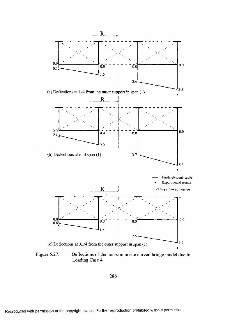
0.00.5,
0.00.0 0.0
2.6
3.8(a) Deflections at L/4 from the outer support in span (1)
R !
0.0 0.00.0 0.0
2.2
(b) Deflections at mid span (1) 3.7
5.3
R
0.00.6
— F i n i t e - e l e m e n t r e s u lt s • E x p e r im e n t a l r e s u lt s
V a lu e s a r e in m il l im e te r s
0.0'
1.5
0:0
(c) Deflections at 3L/4 from the outer support in span (1)
0.0
3.5
Figure 5.27. Deflections o f the non-composite curved bridge model due to Loading Case 4
286
Reproduced with permission of the copyright owner. Further reproduction prohibited without permission.
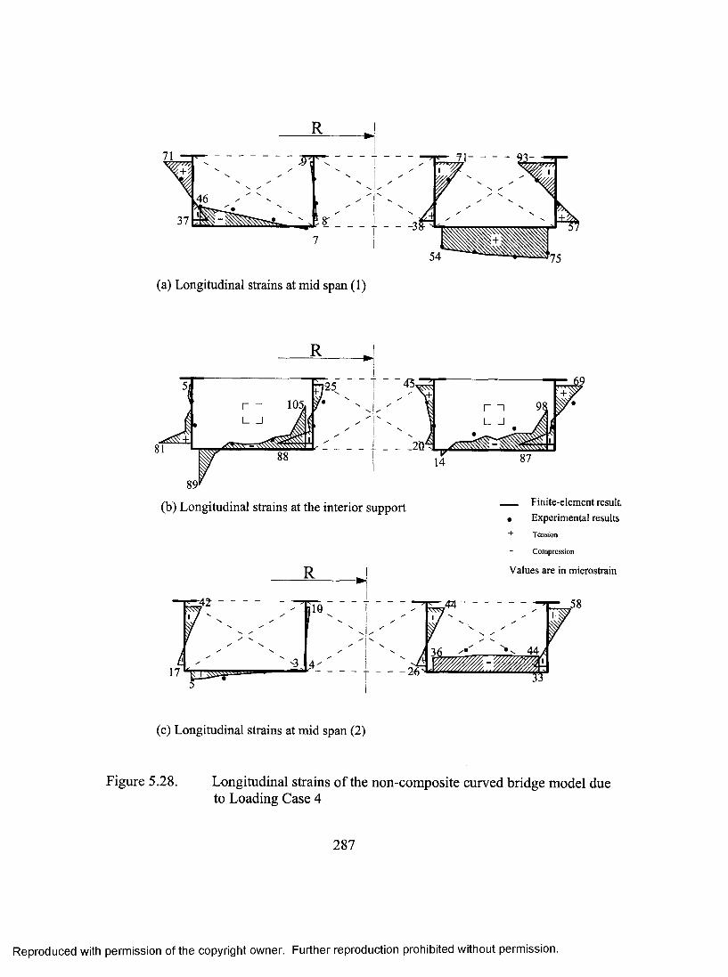
(a) Longitudinal strains at mid span (1)
105,
(b) Longitudinal strains at the interior support F i n i t e - e l e m e n t r e s u l t• E x p e r im e n t a l r e s u lt s+ Tension
Compression
V a lu e s a r e in m ic r o s tr a in
(c) Longitudinal strains at mid span (2)
Figure 5.28. Longitudinal strains of the non-composite curved bridge model due to Loading Case 4
287
Reproduced with permission of the copyright owner. Further reproduction prohibited without permission.
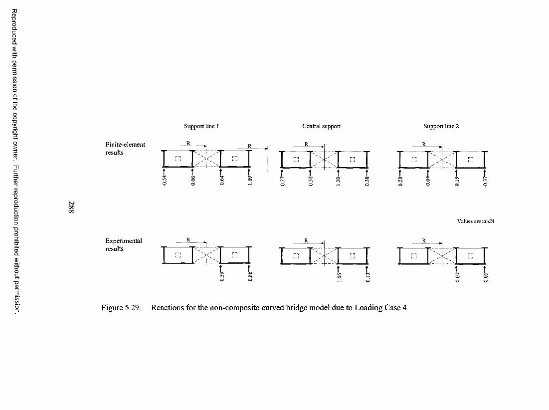
7]CD■DOQ .CoCDQ .
■DCD
C/)Wo'oo
oo■Dcq'
3CD
3"OCD■DOQ .Cao3■oo
CDQ.
■DCD
Finite-elementresults
S u p p o r t l i n e 1
R
C e n t r a l s u p p o r t S u p p o r t l i n e 2
R
cso
00fSo o
boooOOValues are in kN
Experimentalresults
C/)C/)
Figure 5.29. Reactions for the non-composite curved bridge model due to Loading Case 4
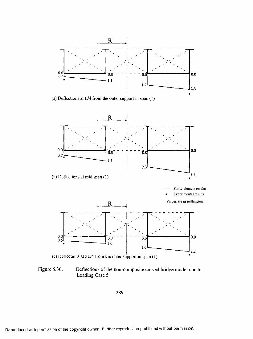
R
0.00.5 o:o-
1.10.0
2.3
(a) Deflections at L/4 from the outer support in span (1)
0.00.7
0.00.0 0.0
2.3
3.2(b) Deflections at mid span (1)
R
— Finite-element results • Experimental results
Values are in millimeters
0.00.5
0.00.0 0.0
2.2(c) Deflections at 3 L/4 from the outer support in span (1)
Figure 5.30. Deflections of the non-composite curved bridge model due to Loading Case 5
289
Reproduced with permission of the copyright owner. Further reproduction prohibited without permission.
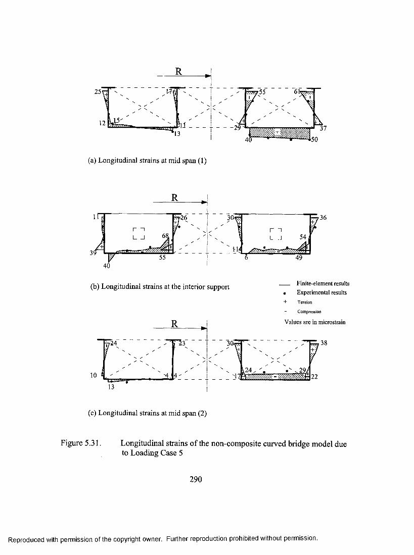
R
25
12
' - ' 1
Iii13
(a) Longitudinal strains at mid span (I)
r36
(b) Longitudinal strains at the interior support
R
10
p i ■ 23 ^
13
F i n i t e - e l e m e n t r e s u lt s• E x p e r im e n t a l r e su lts+ Tension
Compression
V a lu e s a r e in m ic r o s tr a in
r38
22
(c) Longitudinal strains at mid span (2)
Figure 5.31. Longitudinal strains o f the non-composite curved bridge model due to Loading Case 5
290
Reproduced with permission of the copyright owner. Further reproduction prohibited without permission.

CD■DOQ.CoCDQ .
■DCD
C/)Wo'oo
oo■Dc q '
Support line 1 Central support Support line 2
O’oCD■DOQ .CaoQ■oo
CDQ .
"DCD
Finite-elementresults
NJVO
Values are in kl
Experimentalresults
R R
VOo
R
(/)(/)Figure 5.32. Reactions for the non-composite curved bridge model due to Loading Case 5

a) Loading Case 1_l
- 1 4 3 0 --Span 1-
-2145--Span 2 - - 3 5 7 5 —
- J
b) Loading Case 2
(— -1430— r r - - - - ^2145- - 3 5 7 5 -
--------
c) Loading Case 3
- 2 1 4 5 - •1430— r - 1 4 3 0 — r - - - - - ^2145-
--------------^W kN— j—l i k N S ---------------
r
d) Loading pase 4
-2145 - 1 4 3 0 — p l 4 3 0 -
S S E t l ^ v : - :- 2 1 4 5 -
Figure 5.33. Cases of loading for the composite straight bridge model
292
Reproduced with permission of the copyright owner. Further reproduction prohibited without permission.

0.0 0.01 .4
0.00.0
2.2
(a) Deflections at L/4 from the outer support in span (1)
0.0
2.2
0.0
2.6 2 .9
(b) Deflections at mid span (1)— F in ite -e le m e n t resu lts • E x p er im en ta l resu ltsV a lu e s are in m illim e ters
0.00.0 0.01 .3
(c) Deflections at 3L/4 from the outer support in span (1)
Figure 5.34. Deflections of the composite straight bridge model due to Loading Case 1
293
Reproduced with permission of the copyright owner. Further reproduction prohibited without permission.

1 2 6
1 7 8 2 7 1- - 1 - 8 8 - - 2 5 6 -
200 2102 8 0 ? 2 9 4
(a) Longitudinal strains at mid span (1)
6- f^8 2 4 3 2 3 7 .I - - - - - - - - - 1
I _ _ _ _ _ _ I
I - - - - - - - - - 1
2 3 7 1 9 6
(b) Longitudinal strains at the interior support Finite-element results
• Experimental results
+ Tension
CotPpTession
Values are in microstrain
2 5 2 8
5 8! , \6 4 ,
56- 5 5 .161
5 4
(c) Longitudinal strains at mid span (2)
Figure 5.35. Longitudinal strains of the composite straight bridge model due to Loading Case 1
294
Reproduced with permission of the copyright owner. Further reproduction prohibited without permission.
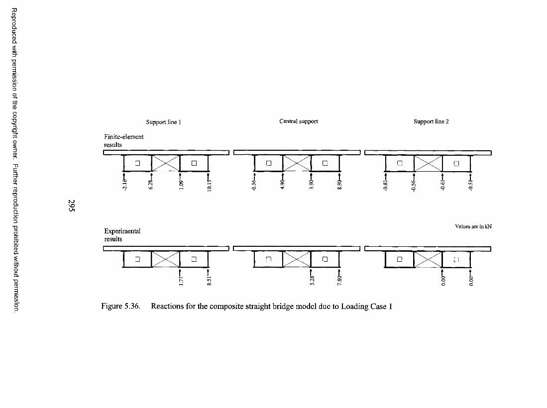
CD■DOQ.CoCDQ .
■ DCD
(/)Wo'o
oo■oc q ’
QCD
CP-O’oCD■oOQ .cao=5
■Oo
CDQ .
Oc■oCD
S u p p o r t l i n e 1 C e n tr a l s u p p o r t S u p p o r t l i n e 2
Finite-elementresults
I C□ X □
> <3 C>
1 r□ □
toVOOl
Experimentalresults
Values are in kN
□ X □ □ X □
o <>
□ X □
oo
oo
(/)o'=3 Figure 5.36. Reactions for the composite straight bridge model due to Loading Case 1
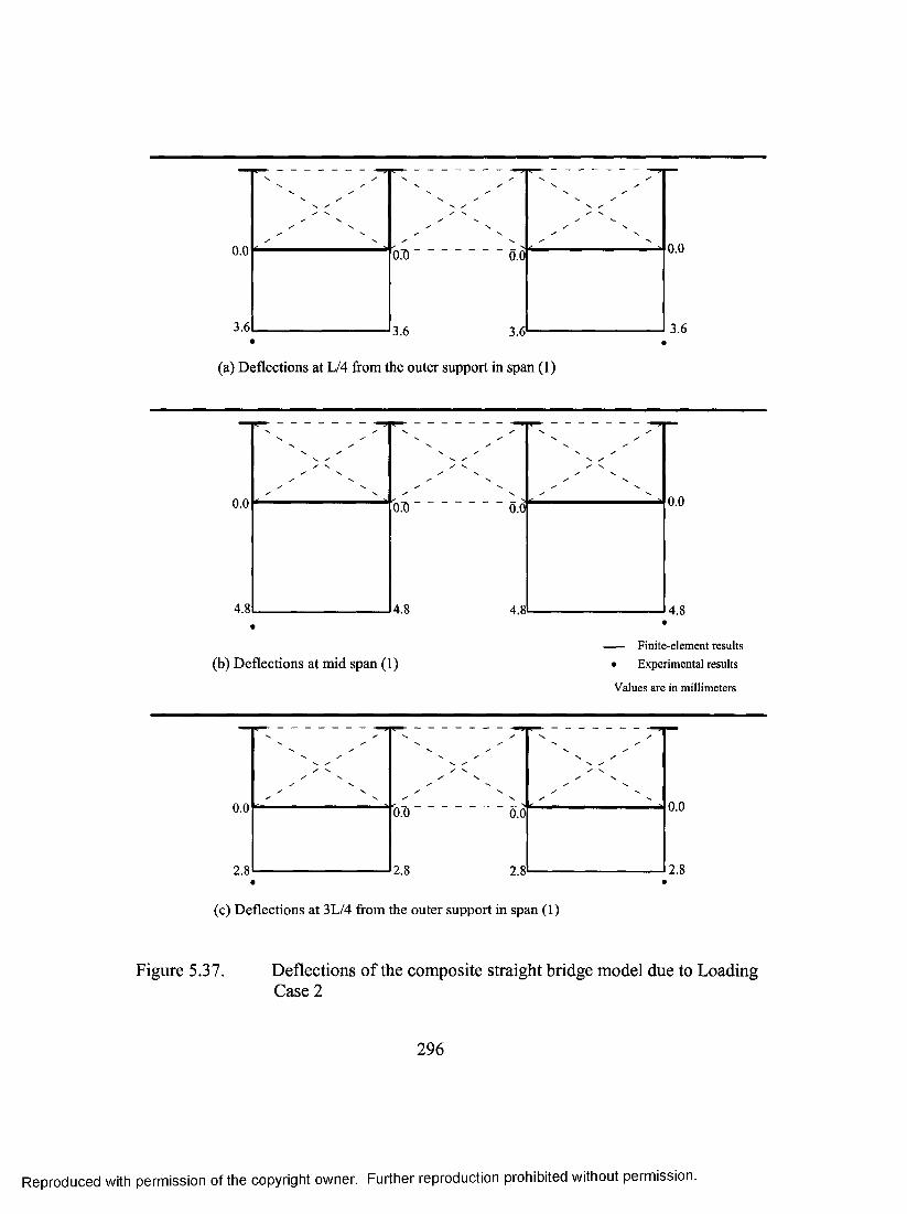
0.0 0.0
3 .6 3 .6
0.00.0
3 .63 .6
(a) Deflections at L/4 from the outer support in span (1)
(b) Deflections at mid span (1)
0.00.0 0.0
4 .8
— Finite-element results
• Experimental results
Values are in millimeters
0.00.0 O.T) 0.0
2.8
(c) Deflections at 3L/4 from the outer support in span (1)
Figure 5.37. Deflections of the composite straight bridge model due to Loading Case 2
296
Reproduced with permission of the copyright owner. Further reproduction prohibited without permission.
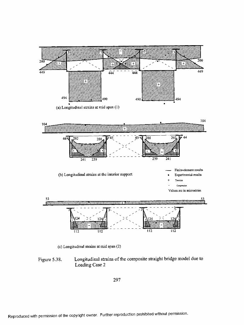
(a) Longitudinal strains at mid span (1)
241 239 239 241
53
(b) Longitudinal strains at the interior support F in ite -e le m e n t resu lts
• E x p e r im e n ta l resu lts+ Tension
Compression
V a lu e s are in m icrostra in
53
.124 124>
112 112112112
(c) Longitudinal strains at mid span (2)
Figure 5.38. Longitudinal strains o f the composite straight bridge model due to Loading Case 2
297
Reproduced with permission of the copyright owner. Further reproduction prohibited without permission.

7JCD■DOQ.CoCDQ .
■DCD
(/)(/)
CD
OO■oS u p p o r t l i n e 1 C e n t r a l s u p p o r t S u p p o r t l i n e 2
Finite-element
CD
CD■DOQ .Cao
results
ON
□ □
j> c 5
] c□ x: □
) r
K)00
T 3
O
CDQ .
T 3CD
Experimentalresults
□ X □] L
□ X □] C
r-On
□ X □
5ooC/)(/)
Figure 5.39. Reactions for the composite straight bridge model due to Loading Case 2
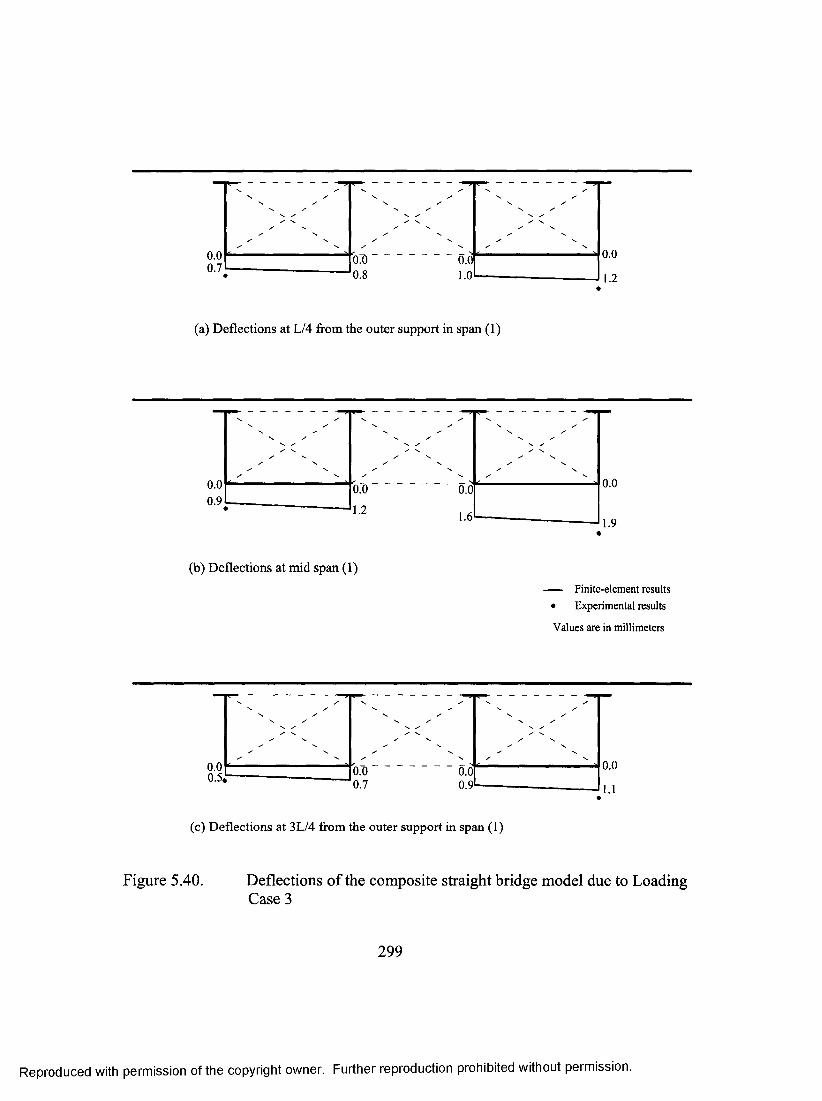
0.00.7
O D0.8
0.01.0-
0.0
1.2
(a) Deflections at L/4 from the outer support in span (1)
0.00.00 .9
0.01.2
(b) Deflections at mid span (1)— F in ite -e le m e n t resu lts • E x p er im en ta l resu ltsV a lu e s are in m illim e ters
0.00 . 5 , O.T)
0 .7
- " " - ^
0 .00 .9
0.01.1
( c ) D e f l e c t i o n s a t 3 L / 4 f r o m t h e o u t e r s u p p o r t i n s p a n ( 1 )
Figure 5.40. Deflections of the composite straight bridge model due to Loading Case 3
299
Reproduced with permission of the copyright owner. Further reproduction prohibited without permission.

1 0 5 i n i75~ 1 9 21 1 6
1 2 8 2 0 6 2 2 3
(a) Longitudinal strains at mid span (1)
1 7 3
4 8 14 3 4
2 4 6 ,,2 0 4
212 1 7 2 3 4 3 3 8 2
(b) Longitudinal strains at the interior support Finite-element results
• Experimental results
+ Tension
Con^ression
Values are in microstrain
1 1 9 * * 1 2 8
( c ) L o n g i t u d i n a l s t r a i n s a t m i d s p a n ( 2 )
Figure 5.41. Longitudinal strains o f the composite straight bridge model due to Loading Case 3
300
Reproduced with permission of the copyright owner. Further reproduction prohibited without permission.
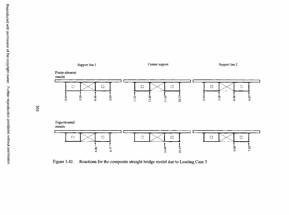
7JCD7DOQ.CoCDQ .
“DCD
(/)(/)
CD
OOTD S u p p o r t l i n e 1 C e n t r a l s u p p o r t S u p p o r t l i n e 2
CD
CD"DOQ .Cao
Finite-elementresults
o
□ □ □ X □
cs o o
U)o
■Do
■DCD
Experimentalresults
ooo
oOn
§3
□ X □ □ X □ □ X □oc
C/)(/)Figure 5.42. Reactions for the composite straight bridge model due to Loading Case 3
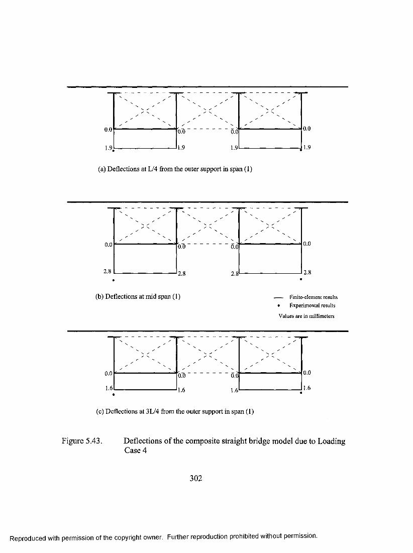
0.00.0 0.0
(a) Deflections at L/4 from the outer support in span (1)
b.T) 0.00.0 0.0
2.8
(b) Deflections at mid span (1) — Finite-element results • Experimental results
Values are in millimeters
0.00.0 0.0
1.6
(c) Deflections at 3L/4 from the outer support in span (1)
Figure 5.43. Deflections o f the composite straight bridge model due to Loading Case 4
302
Reproduced with permission of the copyright owner. Further reproduction prohibited without permission.
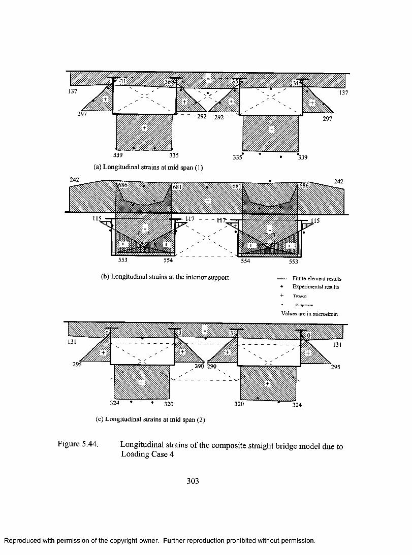
1 3 7 1 3 7
2 9 72 9 7
3 3 9 3 3 5 3 3 5 3 3 9(a) Longitudinal strains at mid span (1)
2 4 2 2 4 2686 6866 8 1
1 1 5 p ^ lT - H7- 1 1 5
5 5 3 5 5 4 5 5 4 5 5 3
(b) Longitudinal strains at the interior support F in ite -e le m e n t resu lts• E x p er im en ta l resu lts+ Tension
Compression
V a lu e s are in m icrostra in
3 2 4 • • 3 2 0
( c ) L o n g i t u d i n a l s t r a i n s a t m i d s p a n ( 2 )
3 2 0 3 2 4
Figure 5.44. Longitudinal strains o f the composite straight bridge model due to Loading Case 4
303
Reproduced with permission of the copyright owner. Further reproduction prohibited without permission.
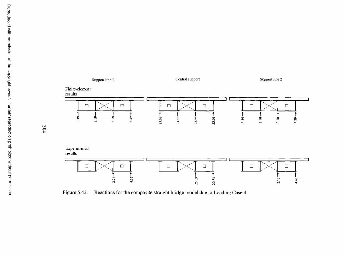
73CD■DOQ.CoCDQ .
■DCD
C/)C/)
OO■Dc q '
S u p p o r t l i n e 1 C e n t r a l s u p p o r t S u p p o r t l i n e 2
O’QCD■DOQ .Cao
Finite-elementresults
□ > c □ □ X □
o
■ao
CDQ .
■DCD
C/)C/)
Experimentalresults
cS
□ X □
Figure 5.45. Reactions for the composite straight bridge model due to Loading Case 4
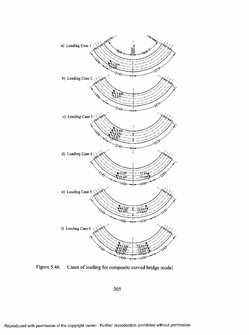
a) Loading Case 1
c) Loading Case 3
b) Loading Case 2 ■, \ \
\ y
d) Loading Case
e) Loading Case
f) Loading Case
Figure 5.46. Cases of loading for composite curved bridge model
305
Reproduced with permission of the copyright owner. Further reproduction prohibited without permission.

R -►I
0.0
2 .5
O.T) t 0.0
3 .34 .0
(a) Deflections at L/4 from the outer support in span (1) R__________^
0.0 0.0
2.63 .4
(b) Deflections at mid span (1)R
0.00.0
4 .45 .3
— F in ite -e le m e n t resu lts • E x p e r im e n ta l resu ltsV a lu e s are in m illim e ters
0.0 0.00.0
2.6( c ) D e f l e c t i o n s a t 3 L / 4 f r o m t h e o u t e r s u p p o r t i n s p a n ( 1 ) •
Figure 5.47. Deflections of the composite curved bridge model due to Loading Case 1
306
Reproduced with permission of the copyright owner. Further reproduction prohibited without permission.
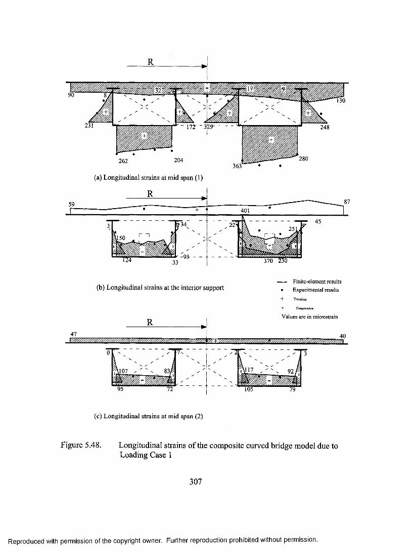
- m - 3 S 9 -
2 6 2 2 0 4
(a) Longitudinal strains at mid span (I)
3 7 0 2 3 0
(b) Longitudinal strains at the interior support Finite-element results
• Experimental results
+ Tension
“ Con^ression
Values are in microstrain
( c ) L o n g i t u d i n a l s t r a i n s a t m i d s p a n ( 2 )
Figure 5.48. Longitudinal strains o f the composite curved bridge model due to Loading Case 1
307
Reproduced with permission of the copyright owner. Further reproduction prohibited without permission.

CD■oOQ .CoCDQ .
■oCD
(/)o '3
OO■ov<c q '
Q.O’oCD■oOQ .caoQ“Oo
CDQ .
TDCD
S u p p o r t l i n e 1 C e n tr a l s u p p o r t S u p p o r t l i n e 2
Finite-elementresults R R R1 1 1 1 1..... ..................... -
□ □ □ □ □ □
oo <N o
OJO00
Experimentalresults
C/)(/)Figure 5.49. Reactions for the composite curved bridge model due to Loading Case 1

R- ► I
0.00.0 0.0
2 .0. 2.2 2 .3
(a) Deflections at L/4 from the outer su|)port in span (1)
0.00.0 0.0
2 .7 2.9
(b) Deflections at mid span (1)
R— F in ite -e le m e n t resu lts • E x p e r im e n ta l resu ltsValues are in millimeters
0.0 b.T) “ “ 0.00.0
( c ) D e f l e c t i o n s a t 3 L / 4 f r o m t h e o u t e r s u p p o r t i n s p a n ( I )
Figure 5.50. Deflections of the composite curved bridge model due to loading Case 2
309
Reproduced with permission of the copyright owner. Further reproduction prohibited without permission.

' - -204 - +236- -
335
66
(a) Longitudinal strains at mid span (I)R
249r -iI I164
123
187 131
34
(b) Longitudinal strains at the interior support
R
— Finite-element results • Experimental results
+ Tension
Compression
Values are in microstrain
28
1--
58/1
65 50
(c) Longitudinal strains at mid span (2)
Figure 5.51. Longitudinal strains of the composite curved bridge model due to Loading Case 2
310
Reproduced with permission of the copyright owner. Further reproduction prohibited without permission.
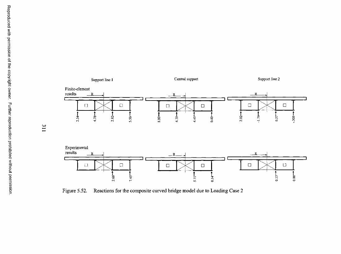
CD“DOQ.CoCDQ .
“DCD
C/)(/)
OO■D(5' S u p p o r t l i n e 1 C e n t r a l s u p p o r t S u p p o r t l i n e 2
CD■aoQ .cao
Finite-element=! results R R R^ 1 1 1------------------------------------ ----------- 1 1 _
■nc3-
□ □ □ □ □ □
rrou>
■ao
CDQ .
■DCD
(/)(/)
Experimental
'OVOfS
results R R R1 i 1 ...................................... ---------------------------1 1
□ □ □ □ □ □
o
o oo o
Figure 5.52. Reactions for the composite curved bridge model due to Loading Case 2

0.00.0 0.0
■----- '4 .65 .4 - — .
I(a) Deflections at L/4 from the outer support in span (1)
- R J
6.2
0.00.0 0.0
5.3
6.27 .3
(b) Deflections at m id span (1)F inite-elem ent results
R • Experim ental results
V alues are in m illim eters
0.00.0 0.0
3 .2
4 .45 .0
(c) Deflections at 3L/4 from the outer support in span (1) ^
Figure 5.53. Deflections of the composite curved bridge model due to Loading Case 3
312
Reproduced with permission of the copyright owner. Further reproduction prohibited without permission.

- t - 3 7 6 -
(a) Longitudinal strains at mid span (1)
2 8 0 5 0 1
(b) Longitudinal strains at the interior support F in ite -e le m e n t resu lts
• E x p er im en ta l resu lts+ Tension
Conq>i«ssion
V a lu e s are in m icrostrain
,201".1 8 0 1 5 9 ,1 4 2 ,
1 5 9 1 8 0
(c) Longitudinal strains at mid span (2)
Figure 5.54. Longitudinal strains of the composite curved bridge model due to Loading Case 3
313
Reproduced with permission of the copyright owner. Further reproduction prohibited without permission.
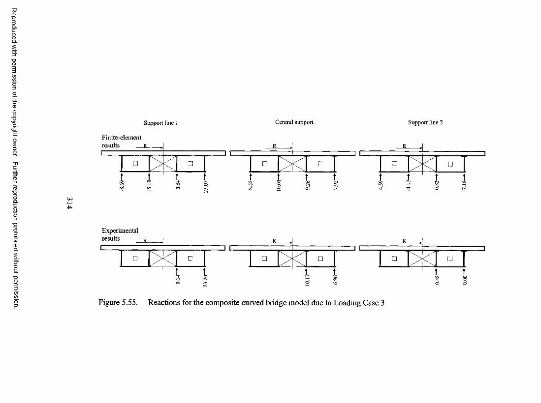
POCD■oOQ.coCDQ .
■oCD
C/)C/)
oo■Dv<cq'
3.
CD■oOQ .cao■Oo
CDQ .
TDCD
C/)C/)
S u p p o r t l i n e 1 Central support S u p p o r t l i n e 2
Finite-element results _
, o
Experimentalresults
Figure 5.55. Reactions for the composite curved bridge m odel due to Loading Case 3

0.00.0
(a) Deflections at L/4 from the outer support in span (1)
R I- ► i
0.01.1
0.0
1.6
0.00.0
2.22.7
(b) Deflections at mid span (1)
R - ► i
— Finite-element results • Experimental results
Values are in millimeters
0.01.2 0.0 T 0.0 0.8 1 1,2
0.0
1.6
(c) Deflections at 3L/4 from the outer support in span (1)
Figure 5.56. Deflections of the composite curved bridge model due to Loading Case 4
315
Reproduced with permission of the copyright owner. Further reproduction prohibited without permission.
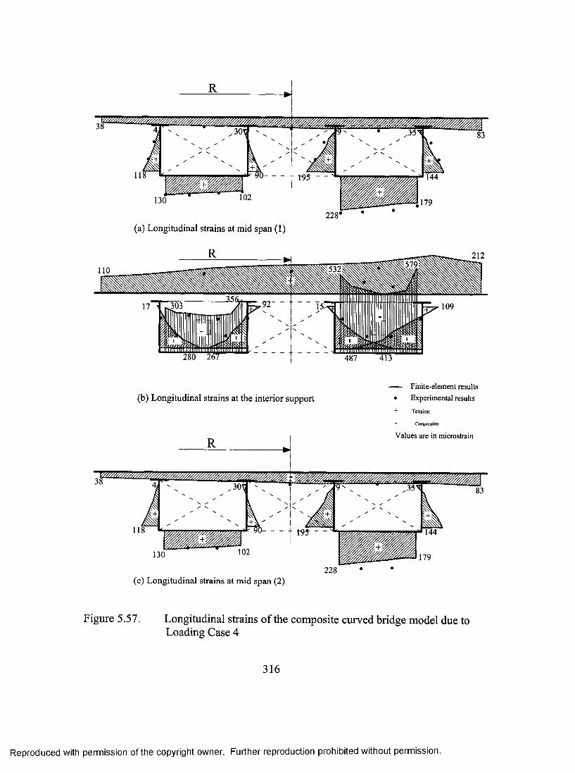
1 1 8 1 4 4
1021 3 0 1 7 92 2 8
(a) Longitudinal strains at mid span (1)
2125 7 91532110
3 0 3
2 8 0 2 6 7 4 1 34 8 7
(b) Longitudinal strains at the interior support F in ite -e le m e n t resu lts
• E x p er im en ta l resu lts+ Tension
Compression
V a lu e s are in m icrostrain
1 1 8 1 4 4
1021 3 0 1 7 92 2 8
( c ) L o n g i t u d i n a l s t r a i n s a t m i d s p a n ( 2 )
Figure 5.57. Longitudinal strains o f the composite curved bridge model due to Loading Case 4
316
Reproduced with permission of the copyright owner. Further reproduction prohibited without permission.

CD■DOQ.CoCDQ .
■DCD
C/)(/)
OO■Dc q '
O’QCD■DOQ .Cao
S u p p o r t l i n e 1 C e n t r a l s u p p o r t S u p p o r t l i n e 2
Finite-element results K
■DO
CDQ .
"DCD
(/)(/)
Experimentalresults
o
J L□ □
o oo o
Figure 5.58. Reactions for the composite curved bridge model due to Loading Case 4
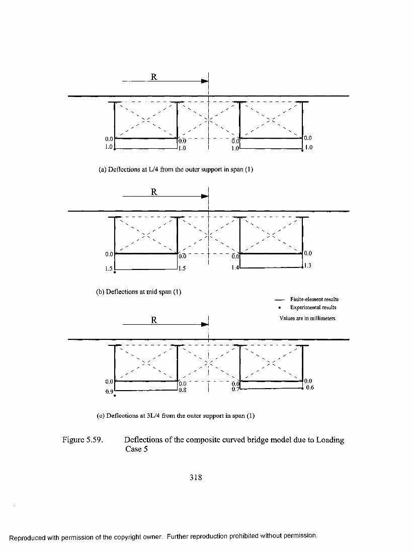
R
0.01.0
0.01.0
0.0l.OL
0.01.0
(a) Deflections at L/4 from the outer support in span (1)
&-----------------.J '
T
0.0 b.T) “ “ o.ol
1.4
0.01.3
(b) Deflections at mid span (1)
R
— Finite-element results • Experimental results
Values are in millimeters- ► I
0.00 . 9
Ti
i. r _____1 ______I s
,
0.0 T 0.0 0.8 i 0.7
0.00.6
( c ) D e f l e c t i o n s a t 3 L / 4 f r o m t h e o u t e r s u p p o r t i n s p a n ( 1 )
Figure 5.59. Deflections o f the composite curved bridge model due to Loading Case 5
318
Reproduced with permission of the copyright owner. Further reproduction prohibited without permission.
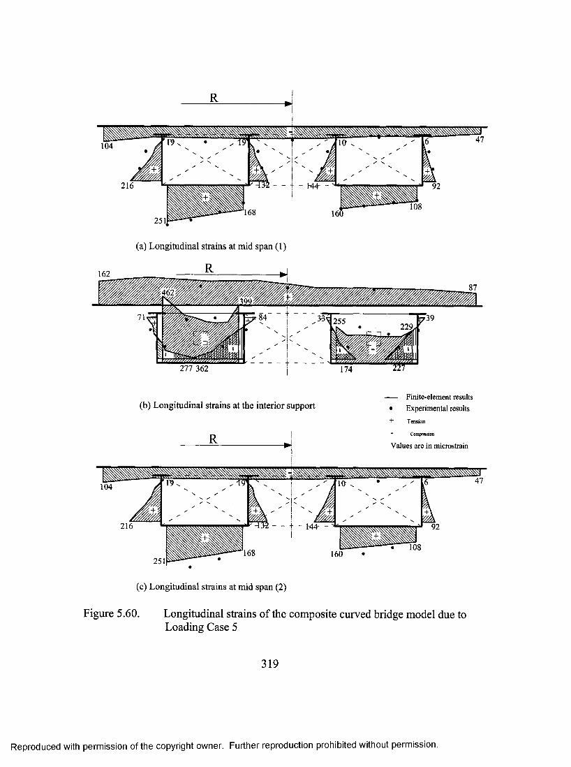
(a) Longitudinal strains at mid span (1)
1211 362
(b) Longitudinal strains at the interior support
R
F in ite -e le m e n t resu lts• E x p er im en ta l resu lts+ Tension
Compression
V a lu e s are in m icrostra in
’ 1 . . w 10 . •" ^ ^^ " V X ^
" i "CM32 - - + - M4- -
251
(c) Longitudinal strains at mid span (2)
Figure 5.60. Longitudinal strains of the composite curved bridge model due to Loading Case 5
319
Reproduced with permission of the copyright owner. Further reproduction prohibited without permission.
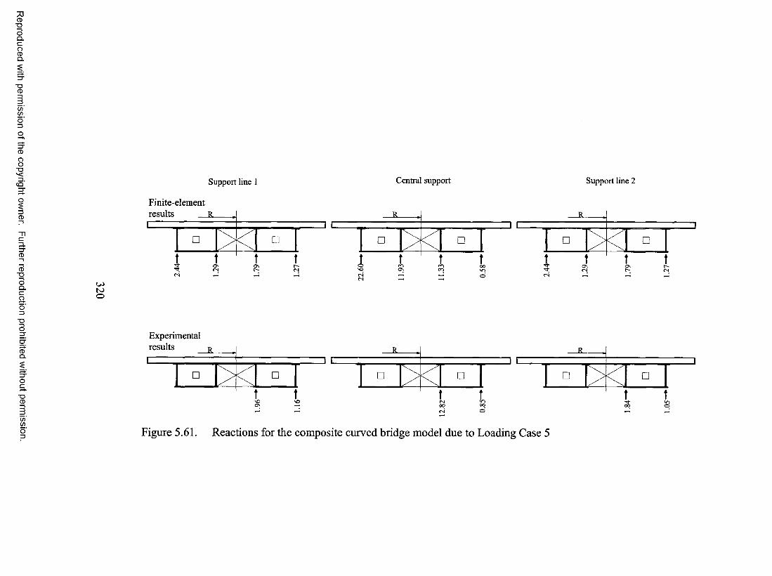
73CD■DOQ.CoCDQ .
■DCD
C/)C/)
OO■Dc q ' S u p p o r t l i n e 1 C e n t r a l s u p p o r t S u p p o r t l i n e 2
Finite-element
O’QCD"DOQ .Cao■oo
CDQ .
■DCD
results
(SU)N)O
Experimentalresults R R
r- 1 1 ■□ □ □ □
w(/)Figure 5.61. Reactions for the composite curved bridge model due to Loading Case 5

0.00.0 0.0
2.2 2 .5
(a) Deflections at ^ from the outer sujpport in span (1)
0.0
2 .7
O.T) t 0.0
3 .64 .0
(b) Deflections at mid span (1)
R
F in ite -e le m e n t resu lts• E x p er im en ta l resu ltsV a lu e s are in m illim e te r s
0.0
1 .5
0:0
1 .7
0.0
1 .9
0.0
2.2
(c) Deflections at 3L/4 from the outer support in span (1)
Figure 5.62. Deflections of the composite curved bridge model due to Loading Case 6
321
Reproduced with permission of the copyright owner. Further reproduction prohibited without permission.

236
388. •381
(a) Longitudinal strains at mid span (1)
■
557 ! 714
(b) Longitudinal strains at the interior support
R I
F in ite -e le m e n t resu lts• E x p er im en ta l resu lts+ Tension
Con^tression
V a lu e s are in m icrostrain
2t9-339
(c) Longitudinal strains at mid span (2)
Figure 5.63. Longitudinal strains of the composite curved bridge model due to Loading Case 6
322
Reproduced with permission of the copyright owner. Further reproduction prohibited without permission.

POCD■oOQ.coCDQ .
■oCD
C/)C/)
oo■ov<c q '
Q.O’QCD■oOQ .CaoQ■oo
CDQ .
TDCD
C/)C/)
S u p p o r t l i n e 1 C e n t r a l s u p p o r t S u p p o r t l i n e 2
Finite-elementresults
ts
U)K)U)
Experimentalresults
O
Figure 5.64. Reactions for the composite curved bridge model due to Loading Case 6
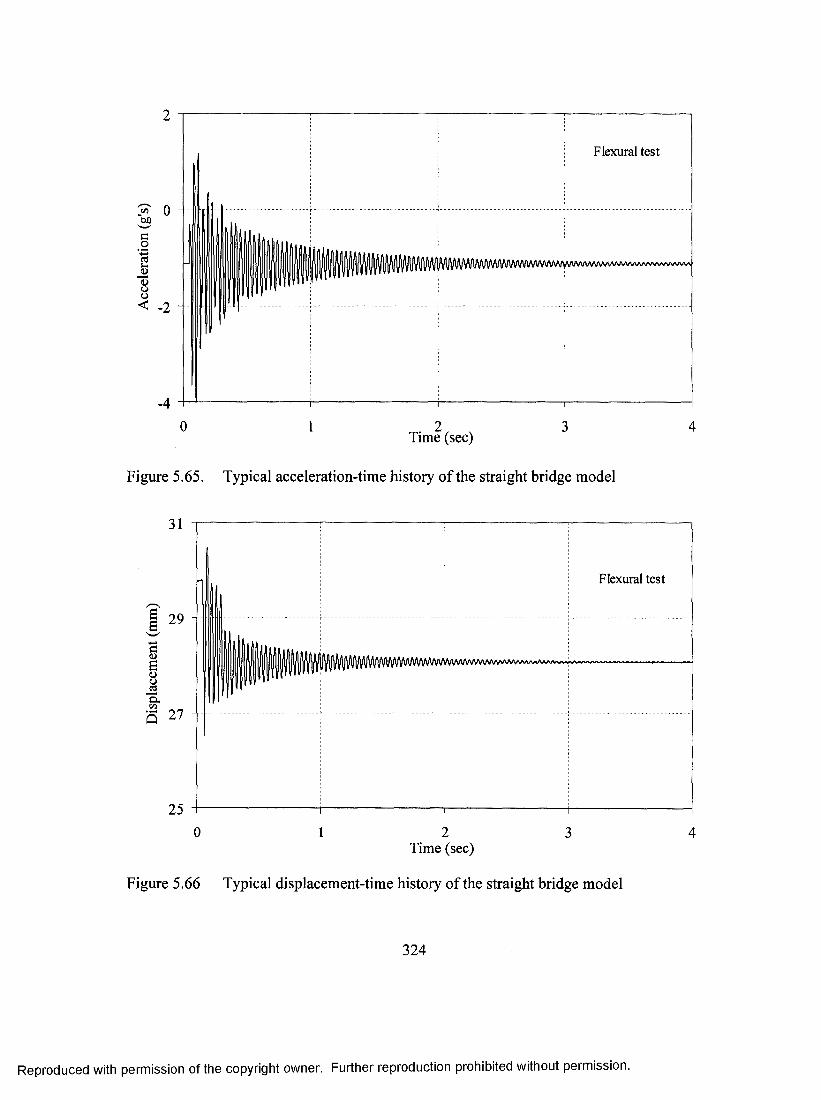
0wc01 13oo< -2
-4
Flexural test
I l l i i i l W i m (\/WWWWSAAAAAaaa/vwwvvw»
'0 1
Time (sec)
Figure 5.65. Typical acceleration-time history of the straight bridge model
Flexural test
(Dsoo—
C/35
0 2 3 41Time (sec)
Figure 5.66 Typical displacement-time history of the straight bridge model
324
Reproduced with permission of the copyright owner. Further reproduction prohibited without permission.

Torsional test
coUt
13oo< -2 -
10 2 3 4Time (sec)
Figure 5.67 Typical acceleration-time history of the curved bridge model
Ss Torsional test
"S
Q29 -
0 2 3 4Time (sec)
Figure 5.68. Typical displacement-time history of the curved bridge model
325
Reproduced with permission of the copyright owner. Further reproduction prohibited without permission.
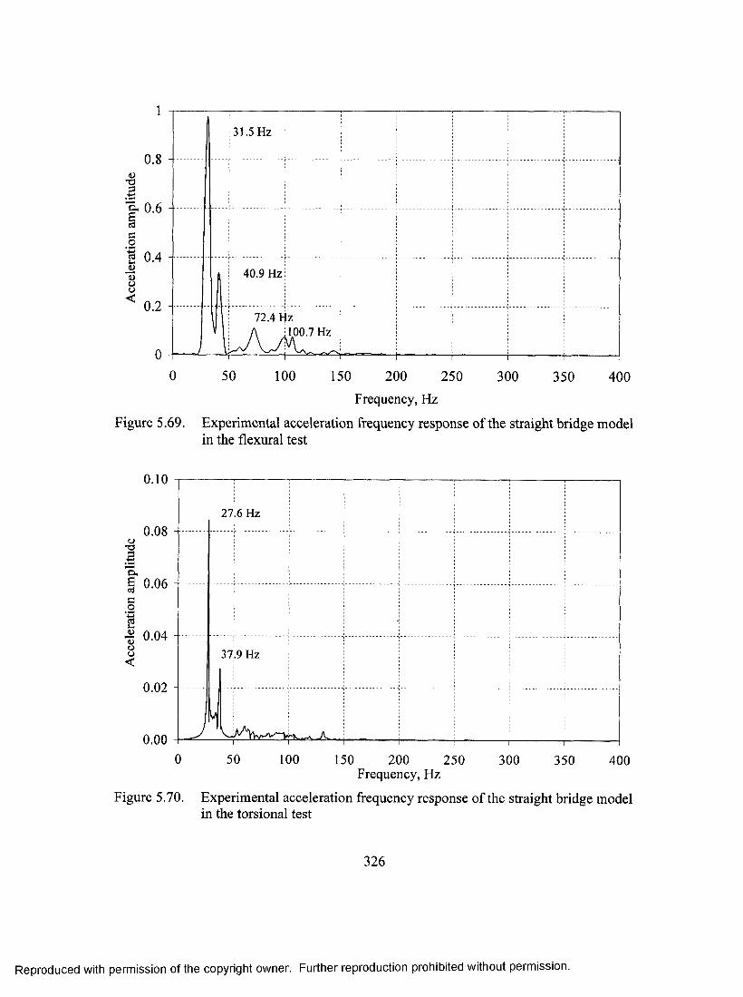
0.8uT33& 0.6edc;.2CS
oo<
0.4
0.2
31.5 Hz
40.9 Hz
___ /
72.4 Fz100.7 Hz
---- -------- 1■ — ■ ■" ...............
0 50 100 150 200 250 300 350 400Frequency, Hz
Figure 5.69. Experimental acceleration frequency response of the straight bridge model in the flexural test
0.10
0.08
I 0-06C01•s 0.04oo<
0.02
0.00
21 .6 Hz
37
1
.9 Hz
J --
50 100 150 200 250 300Frequency, Hz
350 400
Figure 5.70. Experimental acceleration frequency response of the straight bridge model in the torsional test
326
Reproduced with permission of the copyright owner. Further reproduction prohibited without permission.

0.20
3 5 . 0 H z
0.16
I 0.12 -C9.
e 0.08 -1 3oo<
0.04 -
- tN>n00
VO
0.000 50 100 150 200 250 300 350 400
Frequency, Hz
Figure 5.71. Experimental acceleration frequency response of the curved bridge model in the flexural test
0.05
3 4 . 7 H z
0.04<D
^ 0.03ados 0.02
1 3oo<
0.01
7 8 . 6 H z(NVO
0.000 50 100 150 200 250 300 350 400
Frequency, Hz
Figure 5.72. Experimental acceleration frequency response of the curved bridge model in the torsional test
327
Reproduced with permission of the copyright owner. Further reproduction prohibited without permission.

a) Straight bridge model
LAF mode
b) Curved bridge model
LAF-TS mode
Figure 5.73. First and second mode shapes obtained analytically for the bridge models
328
Reproduced with permission of the copyright owner. Further reproduction prohibited without permission.
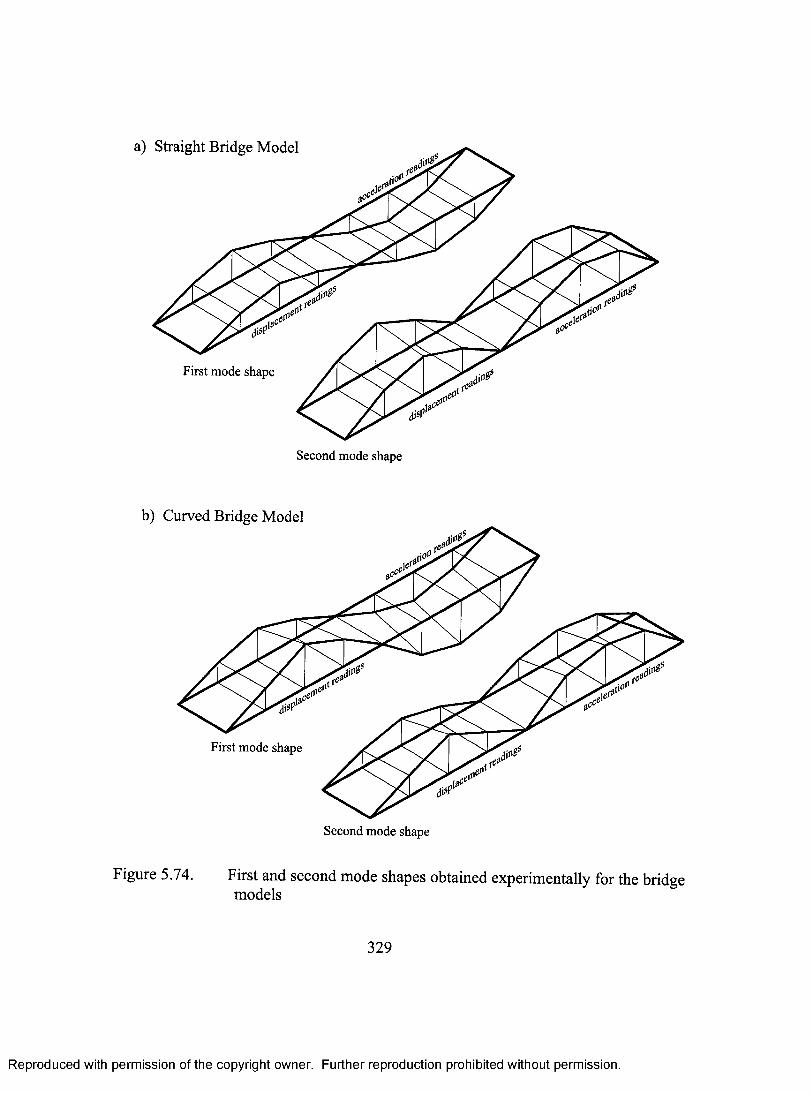
a) Straight Bridge Model
Second mode shape
b) Curved Bridge Model
Second mode shape
Figure 5.74. First and second mode shapes obtained experimentally for the bridge models
329
Reproduced with permission of the copyright owner. Further reproduction prohibited without permission.
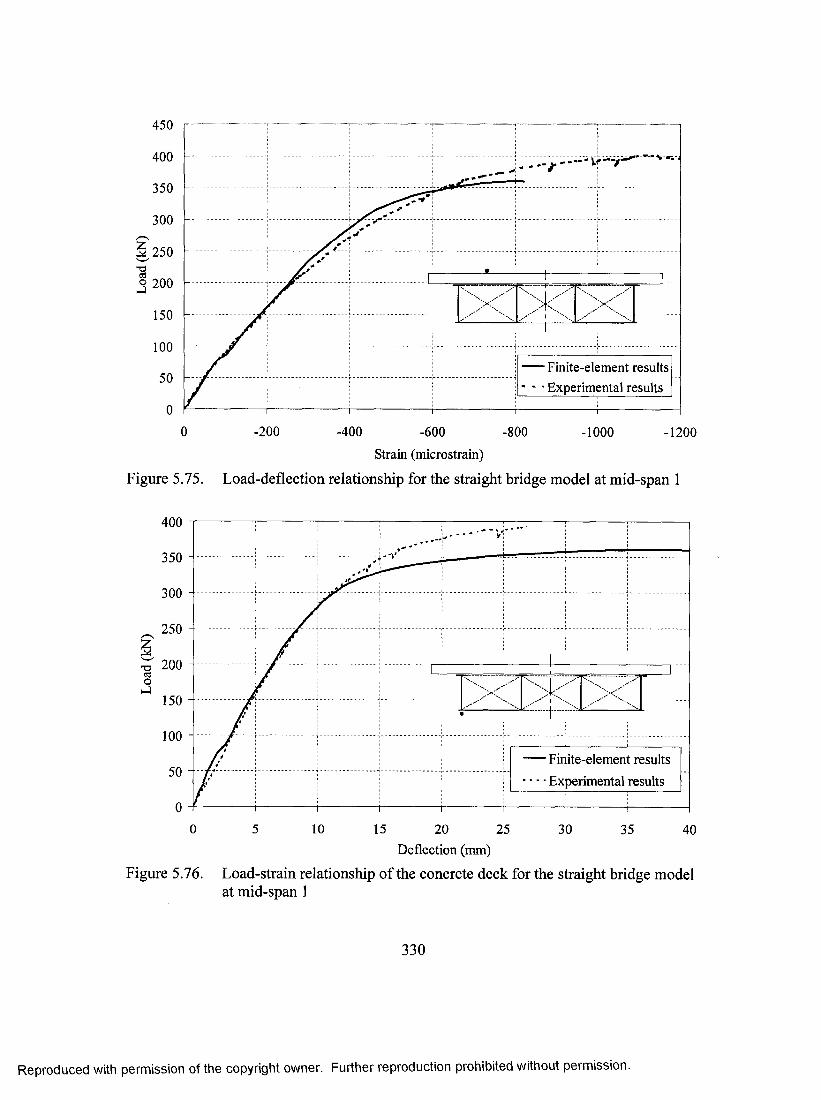
450
400
350
300
2 250
o 200
150
100— Finite-element results- - Experimental results
0 -200 -400 -600 -800 -1000 -1200
Strain (microstrain)
Figure 5.75. Load-deflection relationship for the straight bridge model at mid-span 1
400
350 -
300 -
250
-o 200 - cS O J150 -
100 - Finite-element results Experimental results
50 - -
10 150 5 20 25 30 35 40Deflection (mm)
Figure 5.76. Load-strain relationship of the concrete deck for the straight bridge model at mid-span 1
330
Reproduced with permission of the copyright owner. Further reproduction prohibited without permission.
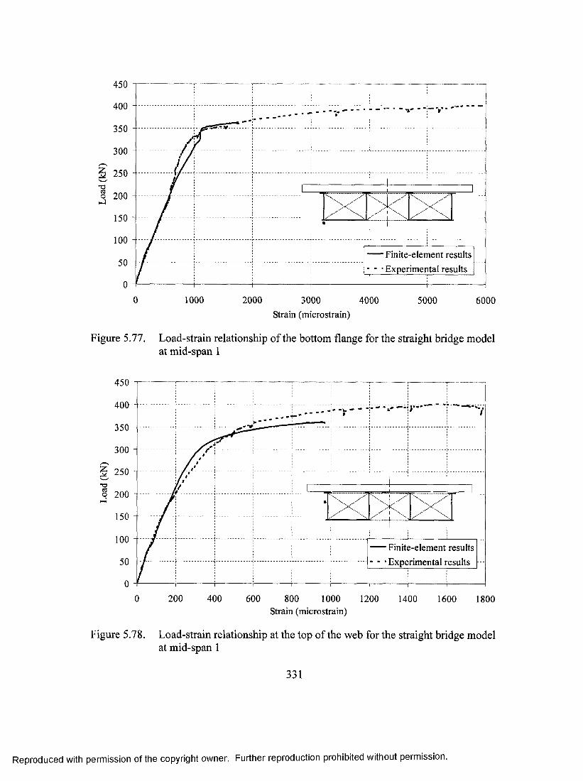
450
400 - V
350
300
250
1 200
150
100 Finite-element results- - • Experimental results
10000 2000 3000 4000 5000 6000Strain (microstrain)
Figure 5.77. Load-strain relationship of the bottom flange for the straight bridge modelat mid-span 1
450
400
350
300
250
150
100— Finite-element results- • Experimental results
0 200 400 600 800 1000 1200 1400 1600 1800Strain (mierostrain)
Figure 5.78. Load-strain relationship at the top of the web for the straight bridge model at mid-span 1
331
Reproduced with permission of the copyright owner. Further reproduction prohibited without permission.
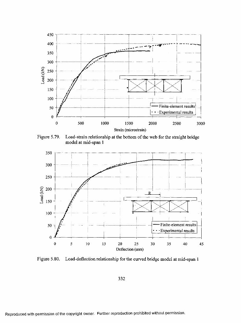
450
400
350
300
s 250
I 200
150
100
Finite-element results- ■ ■ Experimental results
0 500 1000 1500 2000 2500 3000Strain (microstrain)
Figure 5.79. Load-strain relationship at the bottom of the web for the straight bridge model at mid-span 1
350
300
250
J 150
100
— Finite-element results ■ • Experimental results
0 5 10 15 20 25 30 35 40 45Deflection (mm)
Figure 5.80. Load-deflection relationship for the curved bridge model at mid-span 1
332
Reproduced with permission of the copyright owner. Further reproduction prohibited without permission.

350
300
250
z 200
cd^ 150
100
Finite-element results* - • Experimental results
0 10 155 20 25 30 35 40 45 50Deflection (mm)
Figure 5.81. Load-deflection relationship for the curved bridge model at mid-span 1
o-I
350
300
250
200
150
100
Finite-element results • - • Experimental results
50
00 -100 -200 -300 -400 -500 -600 -700 -800 -900
Strain (microstrain)
Figure 5.82. Load-strain relationship of the concrete deck for the curved bridge model at mid-span 1
333
Reproduced with permission of the copyright owner. Further reproduction prohibited without permission.
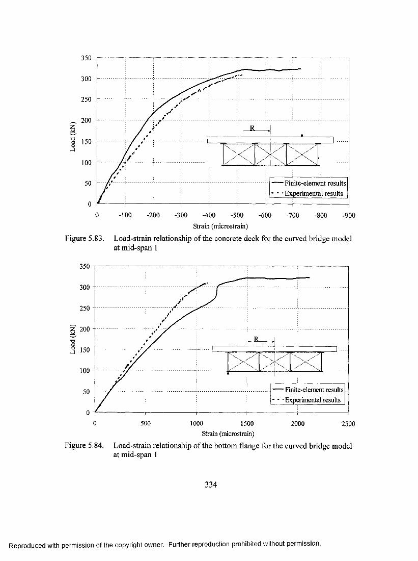
•aISoJ
350
300
250
200
150
100
— Finite-element results • - Experimental results
50
0
0 -100 -200 -300 -400 -500 -600 -700 -800 -900Strain (microstrain)
Figure 5.83. Load-strain relationship of the concrete deck for the curved bridge model at mid-span 1
350
300
250
200
a^ 150
100
— Finite-element results- • Experimental results
0 500 1000 1500 2000 2500Strain (mierostrain)
Figure 5.84. Load-strain relationship of the bottom flange for the curved bridge model at mid-span 1
334
Reproduced with permission of the copyright owner. Further reproduction prohibited without permission.

350
300
250
200
^ 150
100
Finite-element results ■ ■ • Experimental results
0 500 1000 1500 2000 2500Strain (mierostrain)
Figure 5.85. Load-strain relationship of the bottom flange for the curved bridge model at mid-span 1
350
300
250
200
100
Finite-element results‘ - • Experimental results
0 200 1000400 600 800 1200Strain (mierostrain)
Figure 5.86. Load-strain relationship at the top of the web for the curved bridge model at mid-span 1
335
Reproduced with permission of the copyright owner. Further reproduction prohibited without permission.
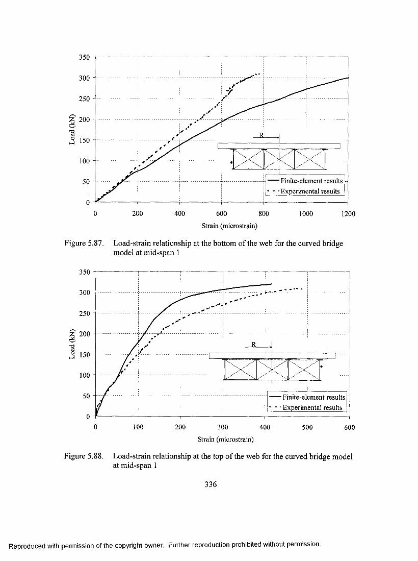
350
300
250
100
Finite-element results• - ■ Experimental results
0 200 400 600 800 1000 1200
Strain (mierostrain)
Figure 5.87. Load-strain relationship at the bottom of the web for the curved bridge model at mid-span 1
350
300
250
200
100
Finite-element results~ - ■ Experimental results
0 100 200 300 400 500 600
Strain (mierostrain)
Figure 5.88. Load-strain relationship at the top of the web for the curved bridge model at mid-span 1
336
Reproduced with permission of the copyright owner. Further reproduction prohibited without permission.
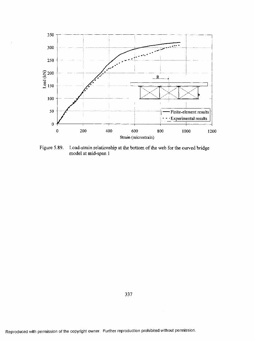
350
300
250
£200T3
^150
100
Finite-element results- ■ • Experimental results
2000 400 600 800 1000 1200Strain (mierostrain)
Figure 5.89. Load-strain relationship at the bottom of the web for the curved bridge model at mid-span 1
337
Reproduced with permission of the copyright owner. Further reproduction prohibited without permission.
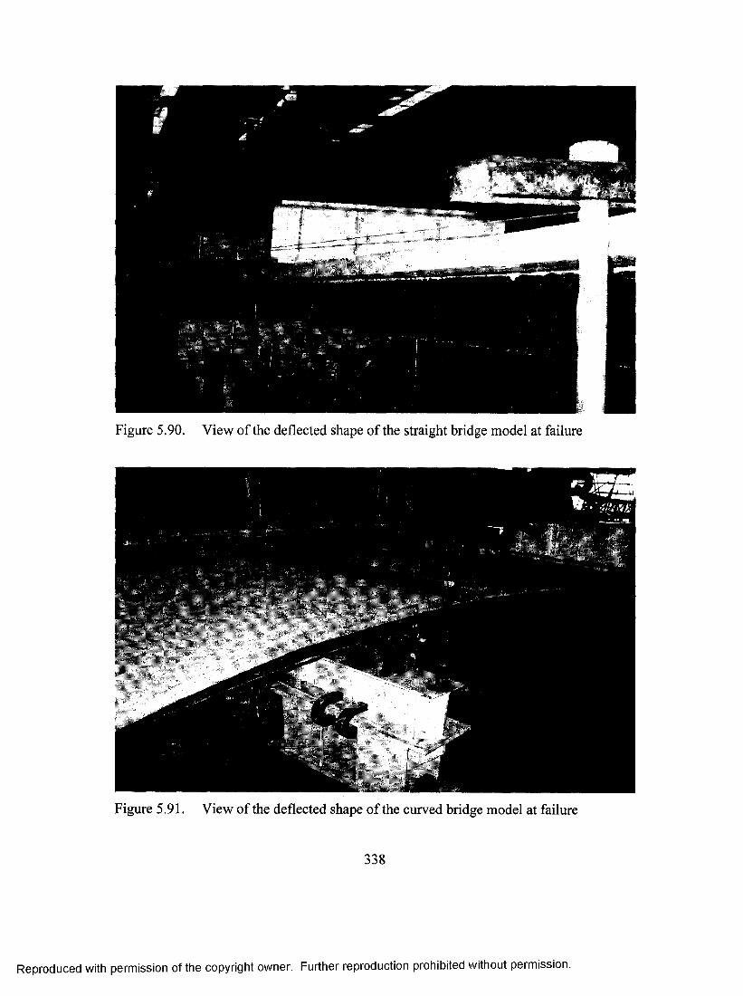
Figure 5.90. View of the deflected shape of the straight bridge model at failure
Figure 5.91. View of the defleeted shape of the curved bridge model at failure
338
Reproduced with permission of the copyright owner. Further reproduction prohibited without permission.
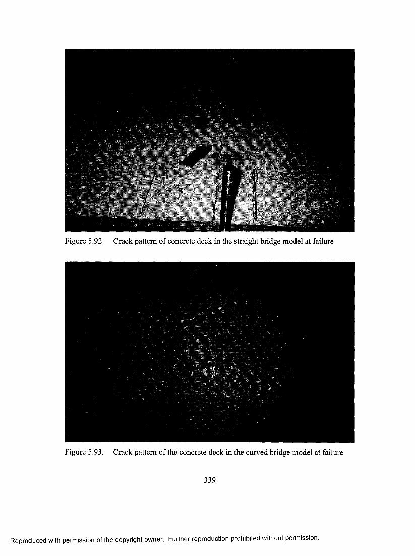
Figure 5.92. Crack pattern of concrete deck in the straight bridge model at failure
Figure 5.93. Crack pattern of the concrete deck in the curved bridge model at failure
339
Reproduced with permission of the copyright owner. Further reproduction prohibited without permission.
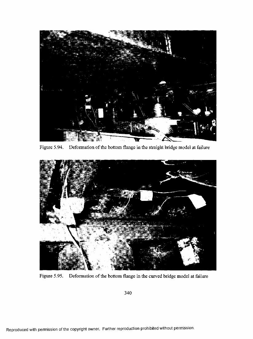
Figure 5.94. Deformation of the bottom flange in the straight bridge model at failure
Figure 5.95. Deformation of the bottom flange in the curved bridge model at failure
340
Reproduced with permission of the copyright owner. Further reproduction prohibited without permission.

H
o.=3o
H
X
CNm
X CQ
X , CQ
X m
x ; om
XCQ
" ' XfN
-23COH
l-H
<L>
T3§
ffiTfo'm<o1/1o
>kHo[L,
o(50■ta
•cX)(U
60XOX5
«4HOc.o
'-Co0t/311/5C/5oIHokH
3oc/3301 00
VO<1
341
pin
Reproduced with permission of the copyright owner. Further reproduction prohibited without permission.
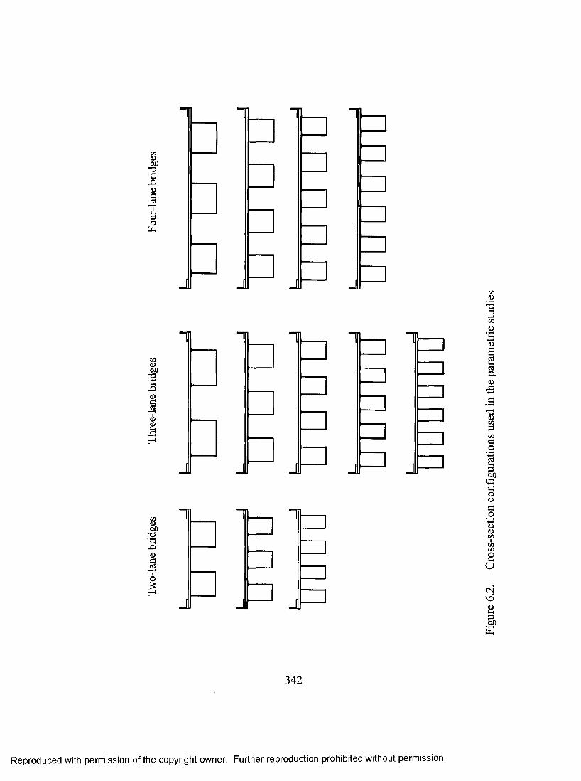
t/1(D
;gDI1ttH
xnu60
;g
II<U
H
(/Iu60
t3■c<uI6H
J
11
J
11
J
1
J1
“I 1 1— 1111
J J J— J 1
JU
1 1
J J
c/5•3hac/5O•£<uaKic3&(U
T30)033i03fl
_o
a
ooa_oo0)030303O)-i
u
CN
a
i-iH
342
Reproduced with permission of the copyright owner. Further reproduction prohibited without permission.

2.0
c
<2
1.5
1.0tjc.2■3I 0.5
Q
(O............. r^ ....... .. i.
Y— ... )[(' .. N ... / ..... .................................
^ Live Load • -G - Dead Load
0.010 20 30
Bottom flange thickness (mm)Figure 6.3. Effect of bottom flange thickness on distribution factor for tensile stress
40
C/5
c<u
oot+3e_oXI
2.0
1.5
1.0
0.5
0.0
Pi.............r
....... ... nS/ ------7i
......... .......... ........................
~)K Live load - -G - Dead load
10 20 30Web thickness (mm)
Figure 6.4. Effect of web thickness on distribution factor for tensile stress
40
343
Reproduced with permission of the copyright owner. Further reproduction prohibited without permission.
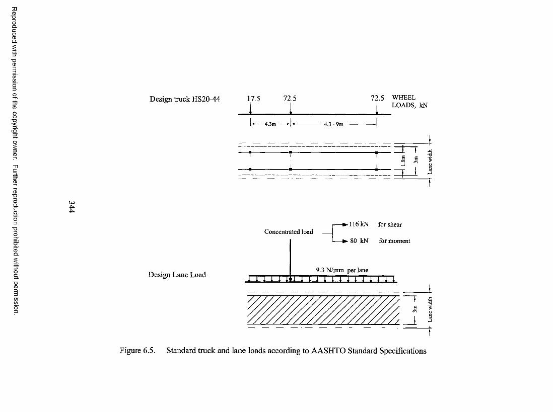
7JCD■DOQ .CoCDQ .
■DCD
(/)(/)
OO■D
Design truck HS20-44 17.51 72.5
J l
72.5 WHEEL I LOADS, kN
k - 4.3 m 4 . 3 - 9 m
CD■DOQ .Cao■oo
CDQ.
■DCD
(/)C/)
Design Lane Load
Concentrated load
n n 1 1
116kN for shear
80 kN for moment
9.3 N/mm per lane1 1 i' 1 1 1 i~l I T ' i i~l 1
,5•O
t
Figure 6.5. Standard truck and lane loads according to AASHTO Standard Specifications
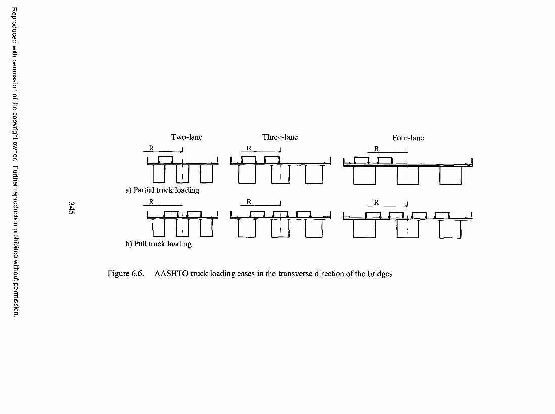
7JCD"DOQ .CoCDQ .
■DCD
(/)(/)
OO■D
3 .
CD■DOQ .C2 .5'3■oo
CDQ .
Oc■oCD
Two-laneR
Three-lane R______ J
Four-lane
R______ JJZIL U □ J U l
UJ
a) Partial truck loading
_R______ J R RJ L r—1 ryi 1— 1 ^ u r—1 r—iif—i m ^
b) Full truck loading
Figure 6.6. AASHTO truck loading cases in the transverse direction o f the bridges
(/)o'o

1
o-cdocd
I<L> .
iS
Pi
J .(DI
t2
(DI
IOsS
Pi
J
Pi
J .
c2>%3c/a011c3a,<u
73<Uli(D3'maoo1/3(L>73C3O60.gC3
P4o
oHmc/2
'O
.1tin
346
Reproduced with permission of the copyright owner. Further reproduction prohibited without permission.

00
l - n “00
u<a
OT3U_N"c3
OS 2
1)bOt3•cX)Xo
•a.N
OJT3
oo
[In
347
Reproduced with permission of the copyright owner. Further reproduction prohibited without permission.

“ I - ; :II "6
r
i f
p
L _
I
i f rE
r
i
r
r
r.aa
oi<Dto
•cX>(L>
C4-1Oa
.2o
.S'O
.2aSia4>
a
M1)MP3O
.s'(J3
O
o£t/3
348
Onv£><D
tL|
Reproduced with permission of the copyright owner. Further reproduction prohibited without permission.

CD■DOQ .CoCDQ .
■DCD
C/)Wo'oo
oo"Dcq '
oCD■DOQ .Caoo■Oo
CDQ .
■DCD
(/)(/)
a) Longitudinal flexure, LF b) Symmetrical torsion, TS c) Combined flexure and torsion, LF-TS
r -
4VO d) Combined longitudinal and transverse flexure, LF-TF
e) Antisymmetric torsion, TAS f) Distortion, DS
^
-h-
^ j i , I ;!u
Original shape Deformed shape at mid-span— Deformed shape at quarter-span
Figure 6.10. Typical mode shapes for two-box girder bridge
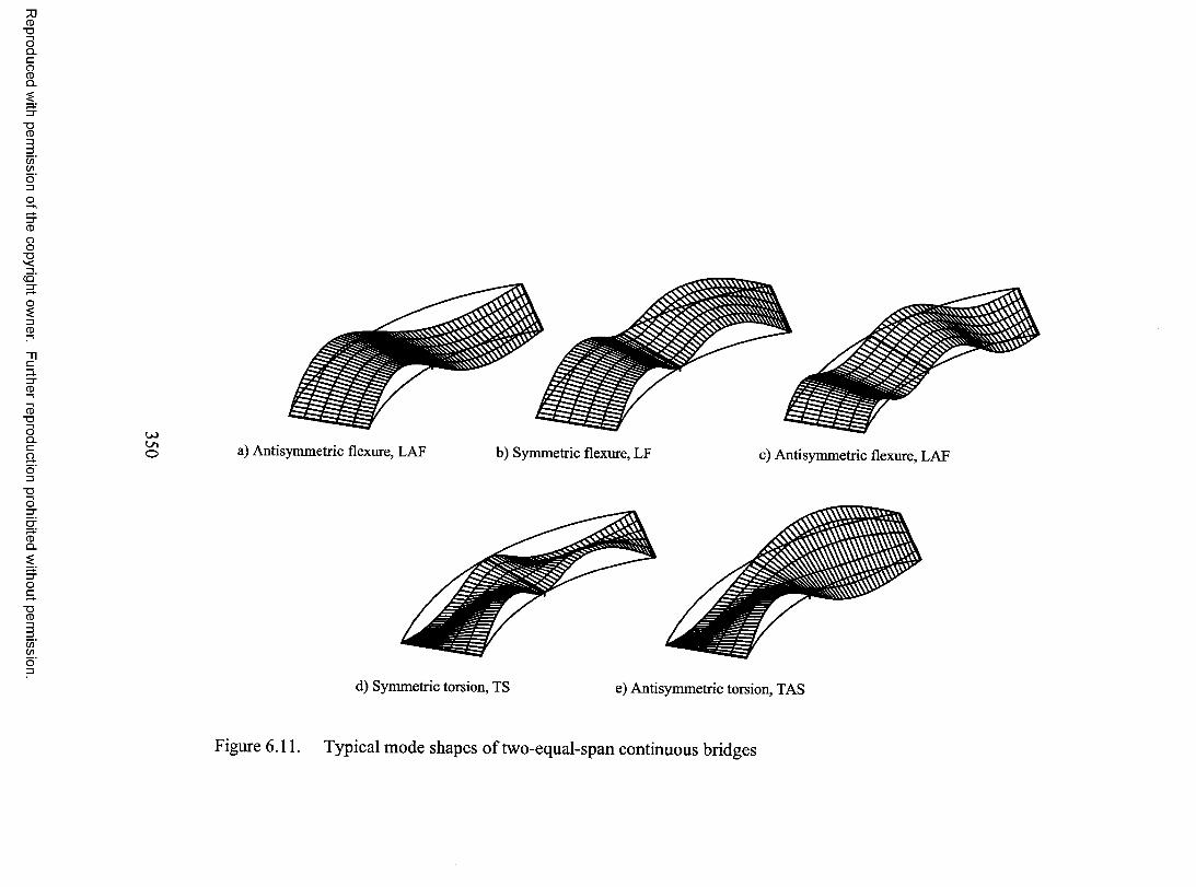
CD■DOQ .CoCDQ .
■DCD
C/)(/)
OO■Dc q '
O’QCD■DOQ .Cao■oo
CDQ .
■DCD
(/)(/)
U>O a) Antisymmetric flexure, LAP b) Symmetric flexure, LF c) Antisymmetric flexure, LAF
d) Symmetric torsion, TS e) Ajitisymmetric torsion, TAS
Figure 6.11. Typical mode shapes o f two-equal-span continuous bridges
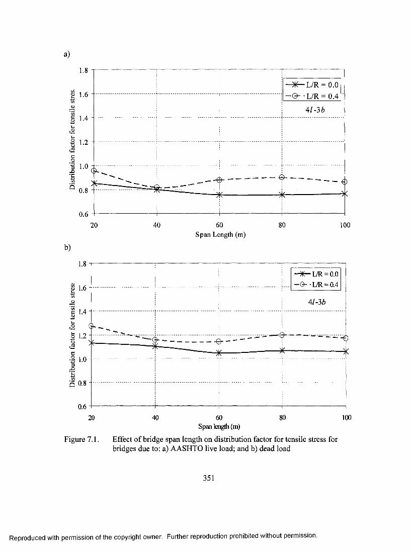
a)
1.8
P 1.6
c/3CCD
u
o-cdd.2px>
1.4
1.2
s .
0.6
■
■ ^ L / R = 0.0 -0- -L/R = 0.4
4l-3b
0 ----- -6)
010 0 (
20 40 60Span Length (m)
80 100
b)
C/3
--------0* ■" —
1.0 -
0.8 -
0.6 480 10020 40 60
Span length (m)
Figure 7.1. Effect of bridge span length on distribution factor for tensile stress for bridges due to: a) AASHTO live load; and b) dead load
351
Reproduced with permission of the copyright owner. Further reproduction prohibited without permission.

a)
^ — L = 20 m 0 - -L = 60 m
c/5<L>
co
Q 0.8 -
0.62 3 4
Number of lanes
b)
1.8
H 1-6
1.4
o 1.2
5 1.0a
15 0.8
0.6
L =20m " O ’ ■L=60m
4b,UK=0A
Qh->e
Number of lanes
Figure 7.2. Effect of number of lanes on distribution factor for tensile stress for bridges due to: a) AASHTO live load; and b) dead load
352
Reproduced with permission of the copyright owner. Further reproduction prohibited without permission.

a)
<D•4
c2UOIc_o'3XI
1.8
1.6
1.4
1.2
1.0
0.8 -
0.6
■ ^ L = 40 m -O -L= 100m
3/,L/R=0.4
0- - - e -o
b)
h.1Qoao3X3
1.8
1.6
1.4 -
1.2
1.0
0.8
0.6
- ^ L = 40m -G- - L= 100 m
3/,I7R = 0.4
Number of boxes
Number of boxes
Figure 7.3. Effect of number of boxes on distribution factor for tensile stress for bridges due to; a) AASHTO live loading; and b) dead load
353
Reproduced with permission of the copyright owner. Further reproduction prohibited without permission.
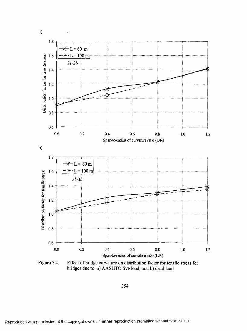
a)
u
l1o
Q
0.60.0 0.2 0.4 0.6 0.8 1.0 1.2
b)
Span-to-radius of curvature ratio (L/R)
- ^ L = 60 m -© --L = 100mg 1.6 -
O
co"3
S 0.8 -
0.60.0 0.2 0.4 0.6 0.8 1.0 1.2
Span-to-radius of curvature ratio (L/R)
Figure 7.4. Effect of bridge curvatiu-e on distribution factor for tensile stress for bridges due to: a) AASHTO live load; and b) dead load
354
Reproduced with permission of the copyright owner. Further reproduction prohibited without permission.

a)
c/5aS8au
Id.2
I
^ L/R = 0.0 0 - -L/R = 0.4
-<)■e-0.8
0.620 40 60 80 100
Span length (m)
b)
0.8 -
0.620 40 60 80 100
Span length (m)
Figure 7.5. Effect of bridge span length on distribution factor for compressive stress bridges due to: a) AASHTO live load; and b) dead load
355
Reproduced with permission of the copyright owner. Further reproduction prohibited without permission.
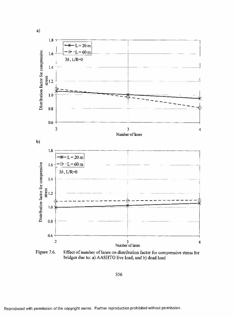
a)
oo
ooco3:2sc/5
1.8
1.6
1.4
c/5C /5
gl.2
5 1.0
0.8
0.6
— —L=20m *L = 60 m
3b,VR=0
b)
QJ.S
oo
o,c§
1.8
1.6
1.4
Sl.2
§ 1-0
0.8 -
0.6
■ ^ L = 2 0 m -©■ -L =60m
36,L/R=0
()"
Number of lanes
Number of lanes
Figure 7.6. Effect of number of lanes on distribution factor for compressive stress for bridges due to: a) AASHTO live load; and b) dead load
356
Reproduced with permission of the copyright owner. Further reproduction prohibited without permission.

a)
X L= 40 m ~ 0 - -L= 100m>
C /3C /3
a.eoo
31, L/R=0.4
so3X)•ccnS 0.8 -
0.62 3 4 5 6
b)
1.8
1.6 -•U&BooucS
1.4
ocSCo
c /3C/5^1-2, C /5
s 1.0 -3x>■£cn
0.8
0.6
Figure 7.7.
Number of boxes
L= 40 m -(>-L=100m
3/,L7R=0.4
(>■•0
Number of boxes
Effect of number of boxes on distribution factor for compressive stress bridges due to: a) AASHTO live load; and b) dead load
357
Reproduced with permission of the copyright owner. Further reproduction prohibited without permission.
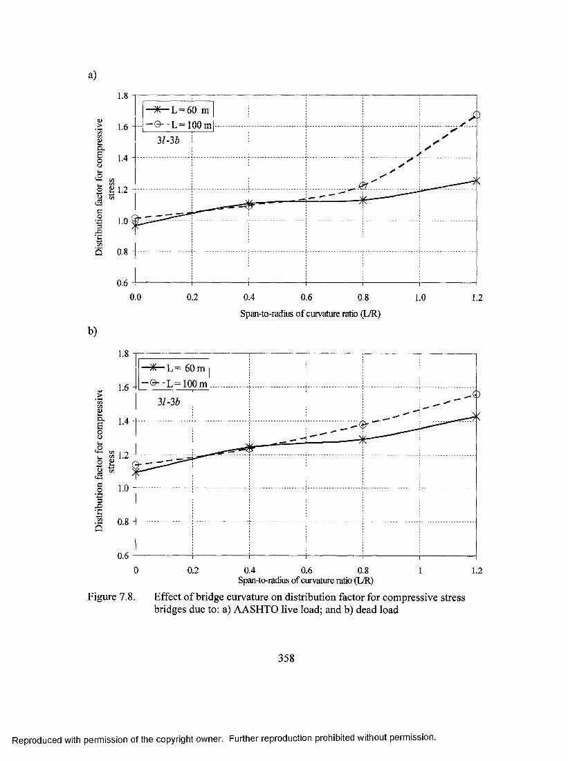
a)
X L= 60 m -0--L=lO O mcu>
'c /2C /30>aSoo
c/3
O 5^
co3
0.60.0 0.2 0.4 0.6 0,8 1.0 1.2
Span-to-radius of curvature ratio (L/R)
b)
•X L= 60 m -©-■L=100m
0.8 -
0.60 0.2 0.4 0.6 0.8 1 1.2
Span-to-radius of curvature ratio (L/R)
Figure 7.8. Effect of bridge curvature on distribution factor for compressive stressbridges due to: a) AASHTO live load; and b) dead load
358
Reproduced with permission of the copyright owner. Further reproduction prohibited without permission.
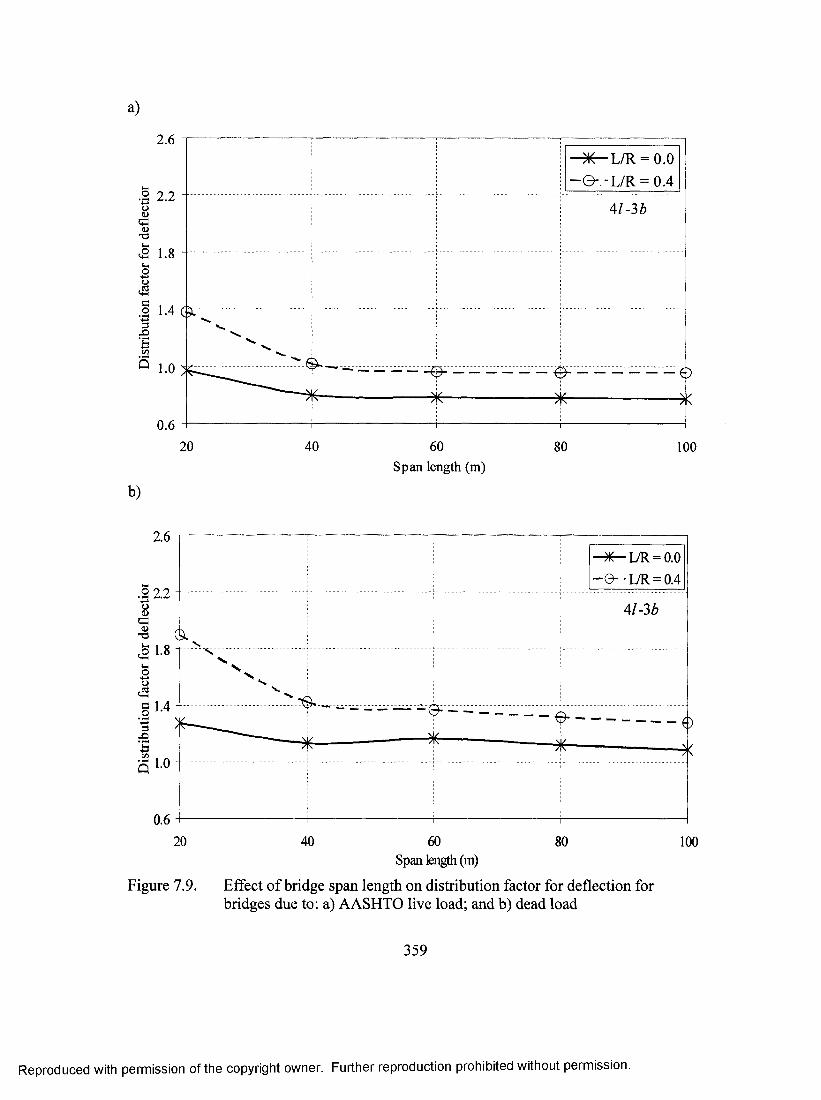
a)
2.6
•2 2.2 O(UCSoT3^ 1.8 u,o
.2 1-4
.oc/3■q 1.0
0.6
- ^ L / R = 0.0 - e - -L /R -0 .4
4l-3b
V. '»s ■V•V,
---- -- J '— — 0
-----------------------^
-..- ............. - .^
.............. —.............. f............. -20 40 60
Span length (m)80 100
b)
2.6- ^ L / R = 0.0 ” <3- -L/R = 0.4
2.2
1.4 -
0.66020 40 80 100
Span length (m)
Figure 7.9. Effect of bridge span length on distribution factor for deflection for bridges due to; a) AASHTO live load; and b) dead load
359
Reproduced with permission of the copyright owner. Further reproduction prohibited without permission.
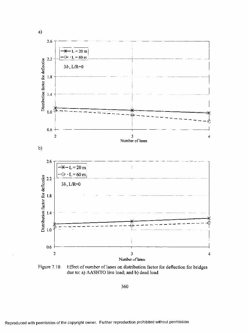
a)
2.6
S 2.2O<D'"O
i01
1.8 -
o 1.43
1.0
0.6
—1— L = 20 m —0 - - L = 60 m
36,L/R=0
■0
Number of lanes
b)
2.6
5 2.2
co
■q
0.62 3 4
Number of lanes
Figure 7.10. Effect of number of lanes on distribution factor for deflection for bridgesdue to: a) AASHTO live load; and b) dead load
360
Reproduced with permission of the copyright owner. Further reproduction prohibited without permission.
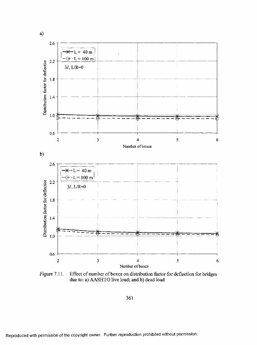
a)
2.6
S 2.2OCdJTS
otj!=:_o
'SU 5
Q
1.8
1.4
1.0
- ^ L = 40m -©--L=100m
3/,L/R=0
(>-
0.6
-ZTZTzi)
b)
Number of boxes
2.6
.2 2.2ooqi3d>•nkH<2kH01<+Hd_o"SXI
- ) ^ L = 40m -e --L = 1 0 0 m
3/,L/R=0
--------------- .■- ~ ---------- ------------------------------- ______ __________^
1.8
1.4
Q 1.0
0.6
Number of boxes
Figure 7.11. Effect of number of boxes on distribution factor for deflection for bridges due to: a) AASHTO live load; and b) dead load
361
Reproduced with permission of the copyright owner. Further reproduction prohibited without permission.
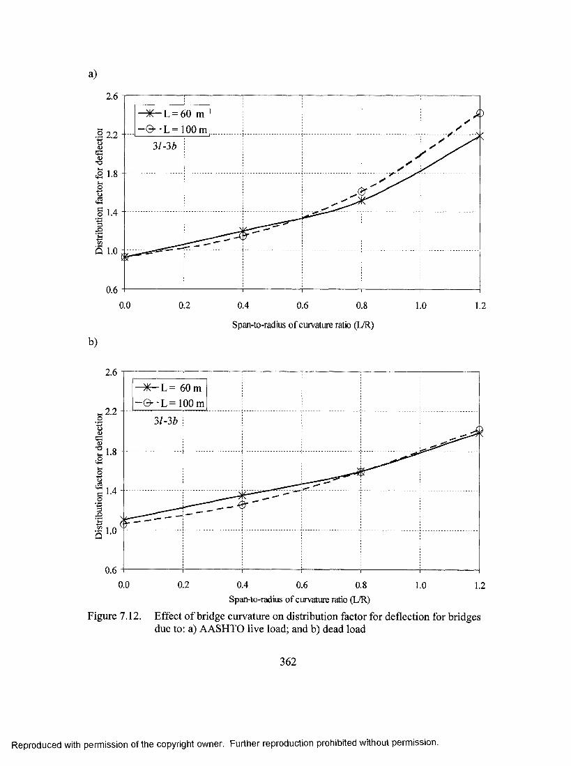
a)
2.6
X L - 60 m - a - L = 1 0 0 m,2 2.2ts0>
<D
OQcoIt o
■q
0.60.0 0.2 0.4 0.6 0.8 1.0 1.2
Span-to-radius of curvature ratio (L/R)
b)
2.6- X - L = 60 m -© -■L=100m
2.2 -
0.60.0 0.2 0.4 0.6 0.8 1.0 1.2
Span-to-radius of curvature ratio (L/R)
Figure 7.12. Effect of bridge curvature on distribution factor for deflection for bridges due to: a) AASHTO live load; and b) dead load
362
Reproduced with permission of the copyright owner. Further reproduction prohibited without permission.

a)
2.6
2.2.s
g l.8 ^IdoS 1.4X )
1.0
0.6
■ ^ L / R = 0.0 -O -L/R = 0.4
4/-3Z)
O
20
----- 1-----
40 60Span length (m)
80 100
b)
2.6
2.2S(D43C/5
‘r l .
dI 'X )■c
.4
1.0
0.6
- ^ L / R = 0.0 -O -L/R = 0.4
4/-3Z>
20 40 60Span length (m)
80 100
Figure 7.13. Effect of bridge span length on distribution factor for shear force for bridges due to: a) AASHTO live load; and b) dead load
363
Reproduced with permission of the copyright owner. Further reproduction prohibited without permission.
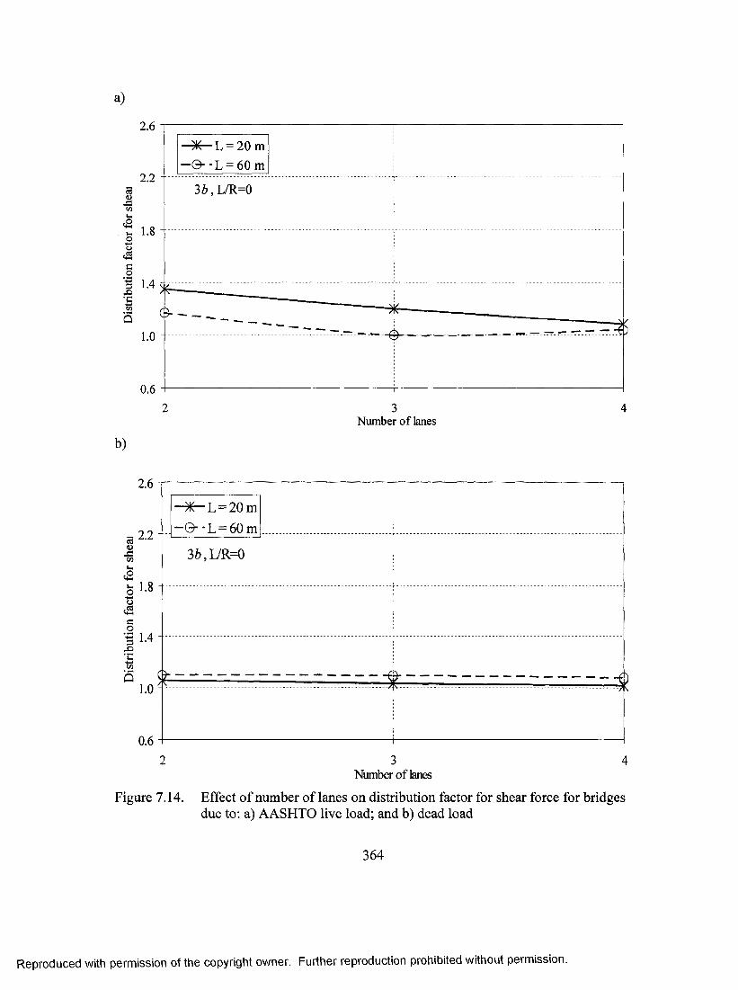
a)
2.6
- ^ L = 20m -© - -L = 60m
2.2 -
OCo3•fi■q
0.62 3 4
Number of lanes
b)
2.6
- ^ L = 20m -©■-L = 60m
3b,L/R=0
_____________________________ ^^ ...................... ......................................- ^
c3C/3
iMc2U2
<4-1
d_o"3x>■£
2.2
1.8
1.4
1.0
0.6
Number of lanes
Figure 7,14. Effect of number of lanes on distribution factor for shear force for bridgesdue to; a) AASHTO live load; and b) dead load
364
Reproduced with permission of the copyright owner. Further reproduction prohibited without permission.
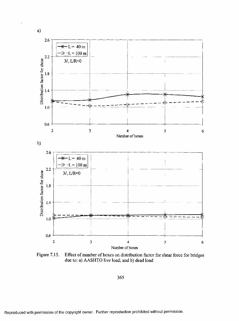
a)
) ^ L = 40 m 0--L=lO O m
3/,L/R=0
b)
ao3X>
2.6
2.2
1.8
1.4
0.6
40m -©- - L= 100 m
3/,L/R=0
4 5Number of boxes
# ■
Number of boxes
Figure 7.15. Effect of number of boxes on distribution factor for shear force for bridges due to: a) AASHTO live load; and b) dead load
365
Reproduced with permission of the copyright owner. Further reproduction prohibited without permission.
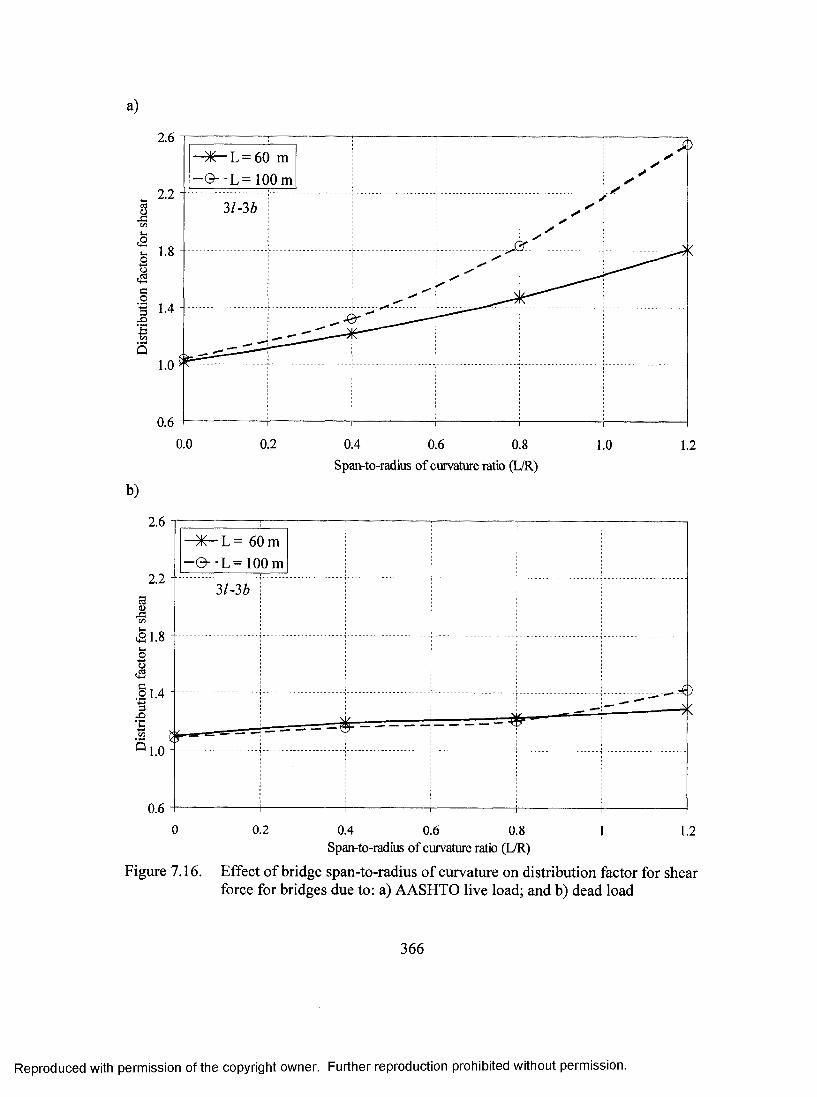
a)
2.6
2.2 -u■S
Ico"3,o
1Q
0.60.0 0.2 0.4 0.6 0.8 1.0 1.2
Span-to-radius of curvature ratio (L/R)
b)
2.6- ) ^ L = 60m -©■ -L - 100m
2.2
0.60 0.2 0.4 0.6 0.8 1.2
Span-to-radius of curvature ratio (L/R)
Figure 7.16. Effect of bridge span-to-radius of curvature on distribution factor for shear force for bridges due to: a) AASHTO live load; and b) dead load
366
Reproduced with permission of the copyright owner. Further reproduction prohibited without permission.

a)
uoaa
.2n><Dt-i<S
Ia.23XI1Q
b)
3.4
3.0
2.6
I 2.2U
1.8
1.4
1.0
>e
20
■ ^ L / R = 0.0 -0- - L/R = 0.4
4/-3 6
0* -O
40 60Span length (m)
80 100
3oo-a3C/2
I
3.4
3.0
2.6 -
3_oSXI1Q
s_o
sa2.2
1.8
1.4
1.0
^ 0 " L /R = O.O _ —0 . -L/R —04 -
4/-3h
0 - ---------------------- ^ ----------------------(---------------------------------------------- -
^ ....- ......20 40 10060 80
Span length (m)
Figure 7.17. Effect of bridge span length on distribution factor for exterior support reaction for bridges due to: a) AASHTO live load; and b) dead load
367
Reproduced with permission of the copyright owner. Further reproduction prohibited without permission.
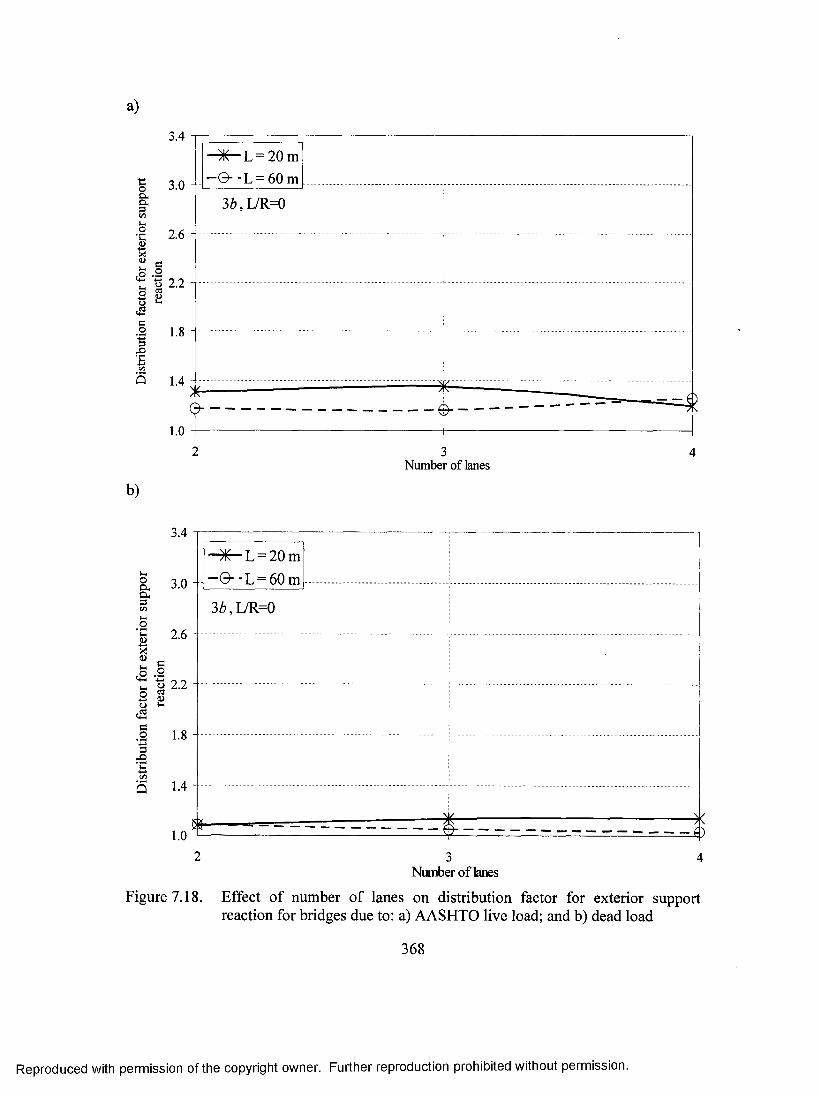
a)
3.4
3.0 - -
2.6 -
2 3 4Number of lanes
b)
oaa-;3
'C%X<uIm
o4-1e,g"3X)’H■q
3.4
3.0
2.6
s01 ui-i
1.8 -
1.4
1.0
~"X L = 20 m ~0- ■L = 60m
3b,UR=0
Number of lanes
Figure 7.18. Effect of number of lanes on distribution factor for exterior support reaction for bridges due to: a) AASHTO live load; and b) dead load
368
Reproduced with permission of the copyright owner. Further reproduction prohibited without permission.
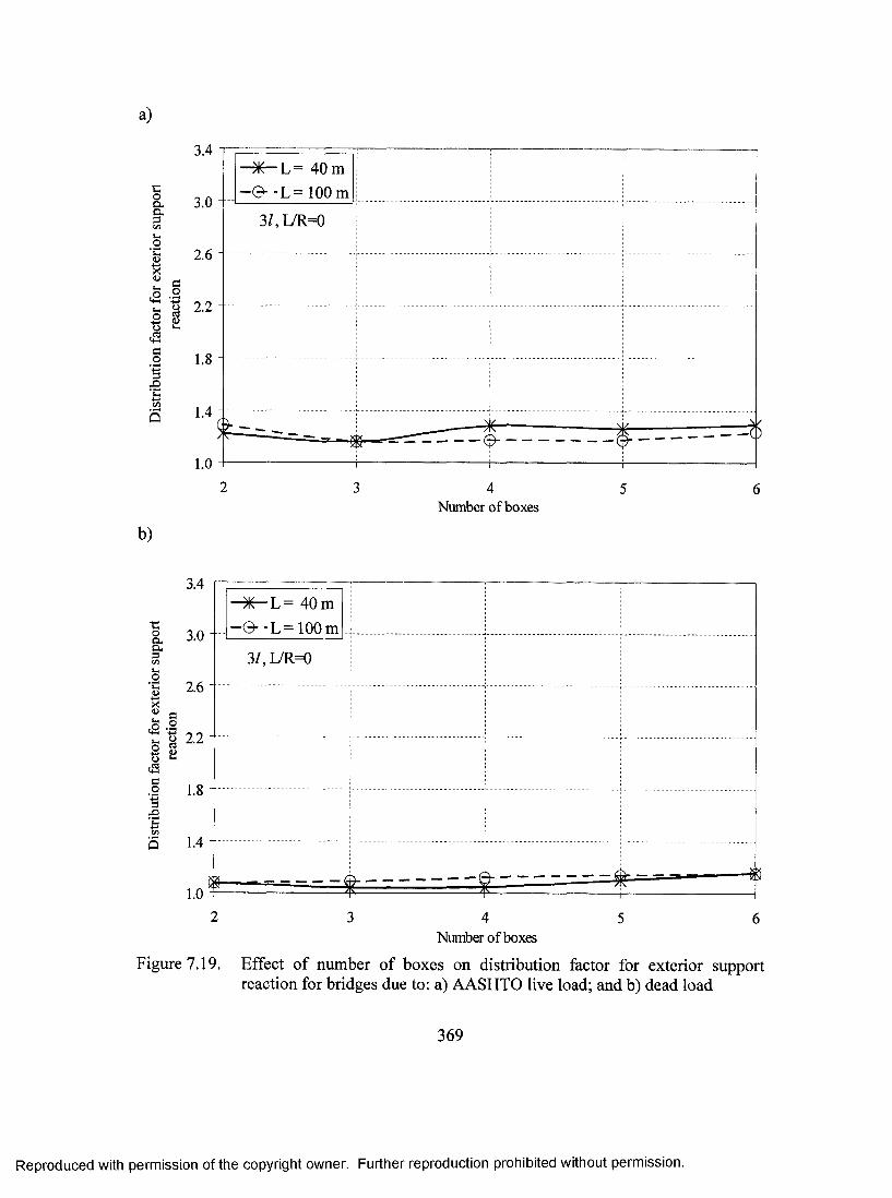
a)
coa .o.3
X0>
3.4
3.0
2.6
^ -2o pMa_o3X)■£t/i
1.8
1.4
1.0
- )K -L = 40m -© - -L= 100m
3/,L/R-0
___ — <--------------- -^ ------------------^ i - - = r z ------------ ---------------------------------------i 1 ' i ...... ........ ........... ..
b)
Number of boxes
t;
§-O*noX<u
01d
_o"3X)15
3.4
3.0
2.6
2.2
1.8
1.4
1.0
X L= 40 m .- e - -L = 1 0 0 m .
3/,L7R=0
§------ ---------------^ ^ ------------- ---— ^ ^
Number of boxes
Figure 7.19. Effect of number of boxes on distribution factor for exterior support reaction for bridges due to: a) AASHTO live load; and b) dead load
369
Reproduced with permission of the copyright owner. Further reproduction prohibited without permission.

a)
3.4
3.0 -D,D.
2.6 -
^ a 2.2 -
0.2 0.40.0 0.6 0.8 1.0 1.2
Span-to-radius of curvature ratio (L/R)
b)
3.4^ L = 60m ©- -L= 100 m3.0 - -
I "X
c(O .2 2.2 - tH-l *3Vh ^% a42co
0.20.0 0.4 0.6 0.8 1.21.0Span-to-radius of curvature ratio (L/R)
Figure 7.20. Effect of bridge curvature on distribution factor for exterior support reaction for bridges due to: a) AASHTO live load; and b) dead load
370
Reproduced with permission of the copyright owner. Further reproduction prohibited without permission.
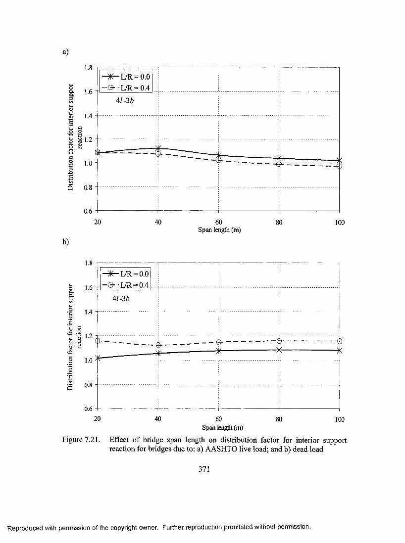
a)
oaPhpc/5UO*c
b)
1.8
1.6
1.4
U<su>
%fCi
C.9"SXi
a01 1.2
1.0
Q 0.8
0.6
L/R =0.0 L/R = 0.4
20
4/-36
40 60Span length (m)
80 100
Uoa.C L3
a;C<2OIHHc.23
X)•c
1.8
1.6
1.4
3_o1<1>
1.2
1.0
0.8
0.6
^ I^ L /R = 0 .0- L/R = 0.4 ---
4/-36
------- ----------- ^
-- ■20 40 80 10060
Span length (m)
Figure 7.21. Effect of bridge span length on distribution factor for interior support reaction for bridges due to; a) AASHTO live load; and b) dead load
371
Reproduced with permission of the copyright owner. Further reproduction prohibited without permission.

a)
ImOcxOhoCOuO•c
Vht2
o,cS-1e.9■3
'BCO
s
- ^ L = 20m —©- -L = 60 m
oocd
0.62 3 4
Number of lanes
b)
Uoo.OnoCO
(L>Vmc2Vhoo,cd
C.2'3x>
1.8
1.6
1.4
c.2<i>
1.2
1.0
0.8
0.6
■ ^ L = 20m "©“ - L = 60 m
Figure 7.22.
36,17R=0
■ 0
3 4Number of lanes
Effect of number of lanes on distribution factor for interior support reaction for bridges due to; a) AASHTO live load; and b) dead load
372
Reproduced with permission of the copyright owner. Further reproduction prohibited without permission.
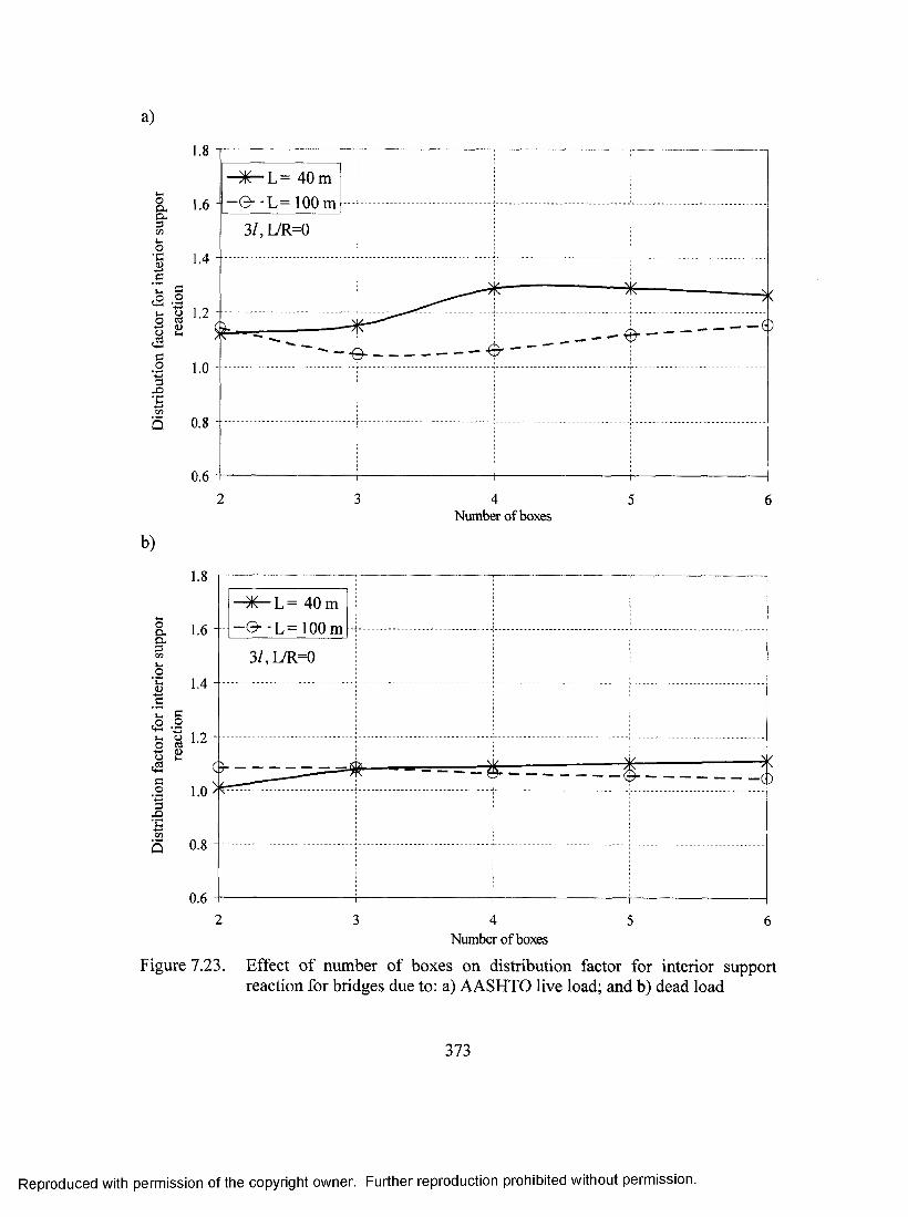
a)
X~" L = 40 m - e - - L = 1 0 0 m
3/,L/R=0
co
- 0
0.62 3 4 5 6
b)
Number of boxes
0 - - L = l O O m
3/,L/R=0
y 1.2
-0
Number of boxes
Figure 7.23. Effect of number of boxes on distribution factor for interior support reaction for bridges due to: a) AASHTO live load; and b) dead load
373
Reproduced with permission of the copyright owner. Further reproduction prohibited without permission.

a)
X L = 60 m -©■-L^lOOm
.2*cfl
2
0.8 -Q
0.6
0 0.2 0.4 0.6 0.8 1 1.2
Span-to-radius of curvature ratio (L/R)
b)
~ X L= 60 m -© ■-L=100m
.s
aX I
'BC/5■q
0.8 -
0.60.0 0.2 0.4 0.6 0.8 1.0 1.2
Span-to-radius of curvature ratio (L/R)
Figure 7.24. Effect of bridge curvature on distribution factor for interior support reaction for bridges due to; a) AASHTO live load; and b) dead load
374
Reproduced with permission of the copyright owner. Further reproduction prohibited without permission.
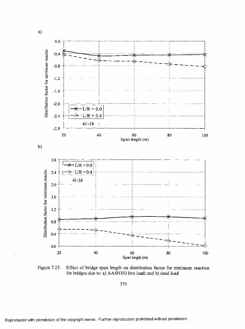
a)
(U
I6’E
o
G.2-2
b)
0.4 C4;
- 1.2
- 1.6
- 2.0
Q -2.4 -
-2.820
-L/R = 0.0-©■ -L/R = 0.4
4 /-3 *
40
“()
60Span length (m)
80 100
E
ISe
<2
GXi■|5
2.8
2.4
2.0
1.6
1.2 -
5 0.8
S 0.4
0.0
X L/R = 0.0 - a - L / R = 0.4
4/-3^»
C>-
20
Figure 7.25.
- X -
-=C)40 60
Span length (m)80 100
Effect of bridge span length on distribution factor for minimum reaction for bridges due to; a) AASHTO live load; and b) dead load
375
Reproduced with permission of the copyright owner. Further reproduction prohibited without permission.

a)
CdssS
0.0
-0.4
-0.8
O -rt-1.2
aos.£5
offj(L>-1.6
-2.0
-2.4
-2.8
.......... - - . . ..... - . . . . . . . . . . . .............. - ........ ..............
)K' L=20 m - 0 - - L = 60m
3Z),L/R=0- - - - - - - - - - - - - - - - - - - - - - - - - - - - - - - - - - - - - - - - - - - - - - - - - - - - - - - - - - - - - - - - - - - - -
Number of lanes
b)
c3scSk.1kH2
C_o3
■£!«
2.8
2.4
2.0
1 1.6
<L>^ 1.2
0.8
0.4 4
0.0
■ ^ L = 20m -Q- -L = 60m
3Z),L/R=0
Number of lanes
Figure 7.26. Effect of number of lanes on distribution factor for minimum reaction for bridges due to: a) AASHTO live load; and b) dead load
376
Reproduced with permission of the copyright owner. Further reproduction prohibited without permission.
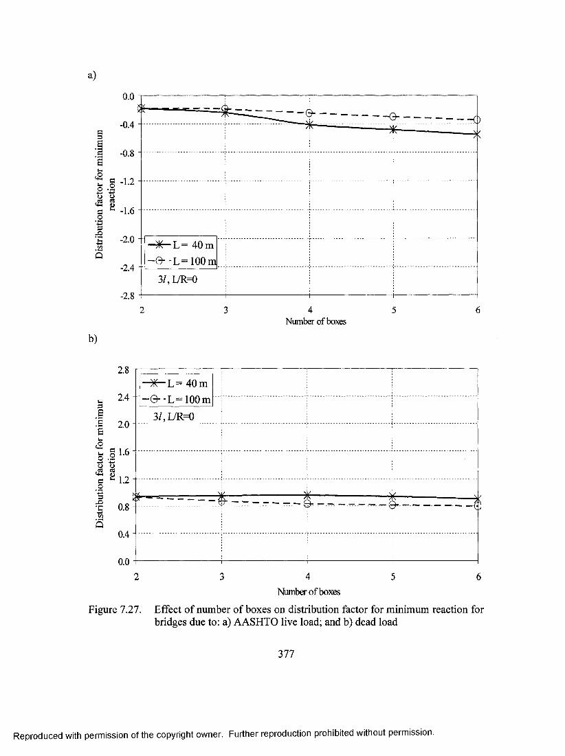
a)
Ssaau,c2Ul
I<4-1c.23
'■§Q
0.0
-0.4 -
-0.8 -
eo
-2.0 - X L= 40m -e - -L = 1 0 0 m-2.4 -
3/,L/R=G-2.8
3 4 62 5Number of boxes
b)
es3
aUi
<2
2.8
2.4
2.0
O .3 1.6
o<4-4c.23
o3 U ^ 1.2
c 0.8
0.4
0.0
- ^ L = 40m -e --L = 1 0 0 m
3/,L/R=0
Number of boxes
Figure 7.27. Effect of number of boxes on distribution factor for minimum reaction for bridges due to: a) AASHTO live load; and b) dead load
377
Reproduced with permission of the copyright owner. Further reproduction prohibited without permission.

a)
■2 0.5
e 0.03e!s -0.5 B
-1.0u01 <+-!3O3 -2.0
(5 -2.5
-3.00.0 0.40.2 0.6 0.8 1.0 1.2
b)
Span-to-radius of curvature ratio (L/R)
0.5o
0.0
§ -0.53B
-1.0
X L = 60 m -© -■L=100m■” -2 5
-3.00.0 0.2 0.4 0.6 0.8 I.O 1.2
Span-to-radius of curvature ratio (L/R)
Figure 7.28. Effect of bridge curvature on distribution factor for minimum reaction for bridges due to; a) AASHTO live load; and b) dead load
378
Reproduced with permission of the copyright owner. Further reproduction prohibited without permission.
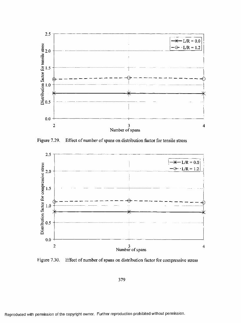
2.5
<U2.0
cuI 1.5
%
§1.0
q O.5
■ *-L /R = 0.0 -0- - L/R = 1.2
- e -
0.02 3
Number of spans
Figure 7.29. Effect of number of spans on distribution factor for tensile stress
2.5
2.0
ai<L>DV 5•!>Cl,t l . 5o0
1 1.0
c ^
I 0.5
Q0.0
C)- -0 -
-L/R = 0.0— 0 _ ■L/R = 1.2
-0
Number of spans
Figure 7.30. Effect of number of spans on distribution factor for compressive stress
379
Reproduced with permission of the copyright owner. Further reproduction prohibited without permission.

2.5
.2 2.0 ts<u0)*oI 1.50OcfS1 1.0 '3X)
(>-
n 0.5
0.0
-L/R = 0.0- 0 - ■L/R = 1.2
- o
Figure 7.31.
2.5
Number of spans
Effect of number of span on distribution factor for deflection
2.0<Dc/5u
1.oa
.2 1.0 3
.1Q o.5
0.0
-L/R = 0.0—0- ■L/R = 1.2
Number of spans
Figure 7.32. Effect of number of spans on distribution factor for shear force
380
Reproduced with permission of the copyright owner. Further reproduction prohibited without permission.

2.5d.9
-ds,&COU|O
<1>
a.9'3
1Q
0
2.0
1.5
1.0
0.5L/R = 0.0
-0 - -L/R= 1.20.0
Number of spans
Figure 7.33. Effect of number of spans on distribution factor for exterior support reaction
OCQd>u*tioaOh
o,ai
2.5
2.0
.9 1.5 -
1.0
do0.5
XI
0.0
L/R = 0.0 -O- -L/R= 1.2
Number of spans
Figure 7.34. Effect of number of spans on distribution factor for interior support reaction
381
Reproduced with permission of the copyright owner. Further reproduction prohibited without permission.
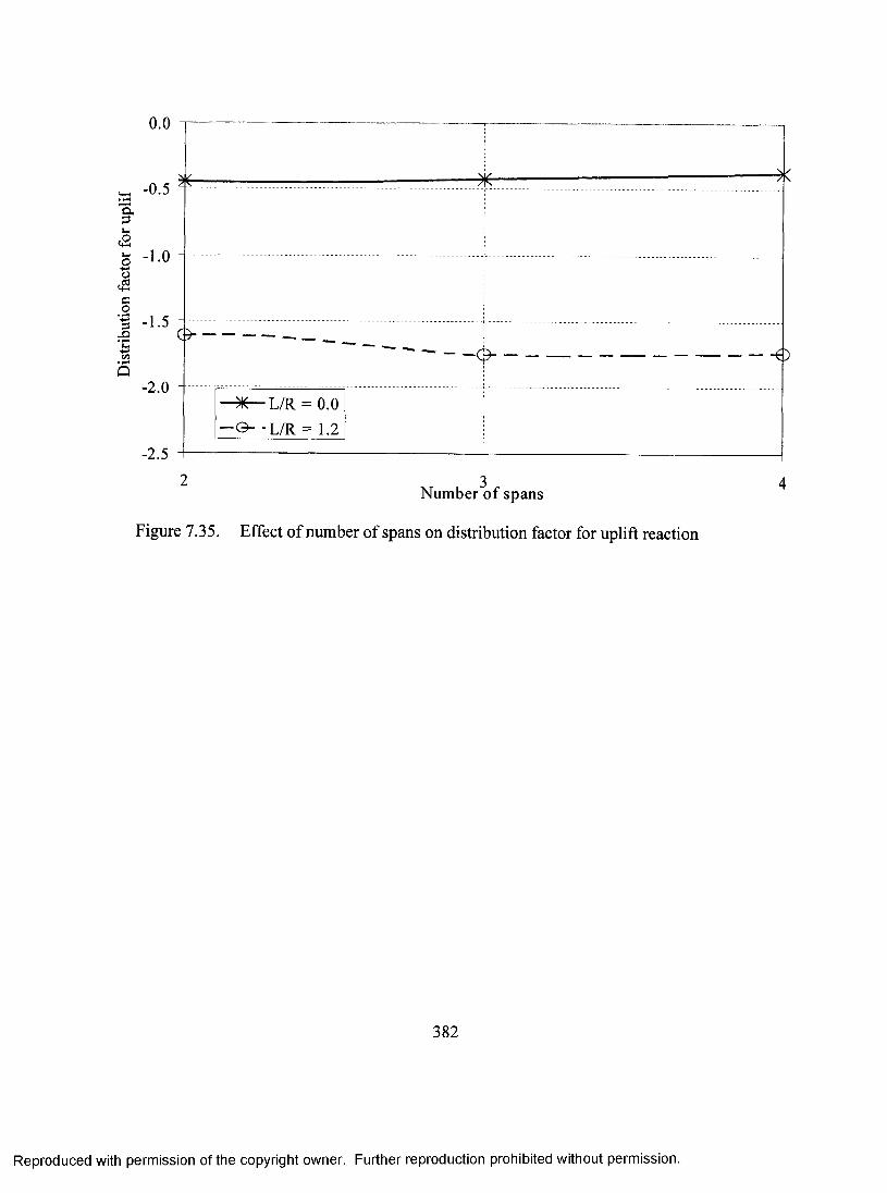
0.0
-0.5
a
i<4-1c
.2"3XIID
-1.0
-1.5
-2.0
-2.5
-L/R = 0.0— &- -L/R = 1.2
Number of spans
Figure 7.35. Effect of number of spans on distribution factor for uplift reaction
382
Reproduced with permission of the copyright owner. Further reproduction prohibited without permission.
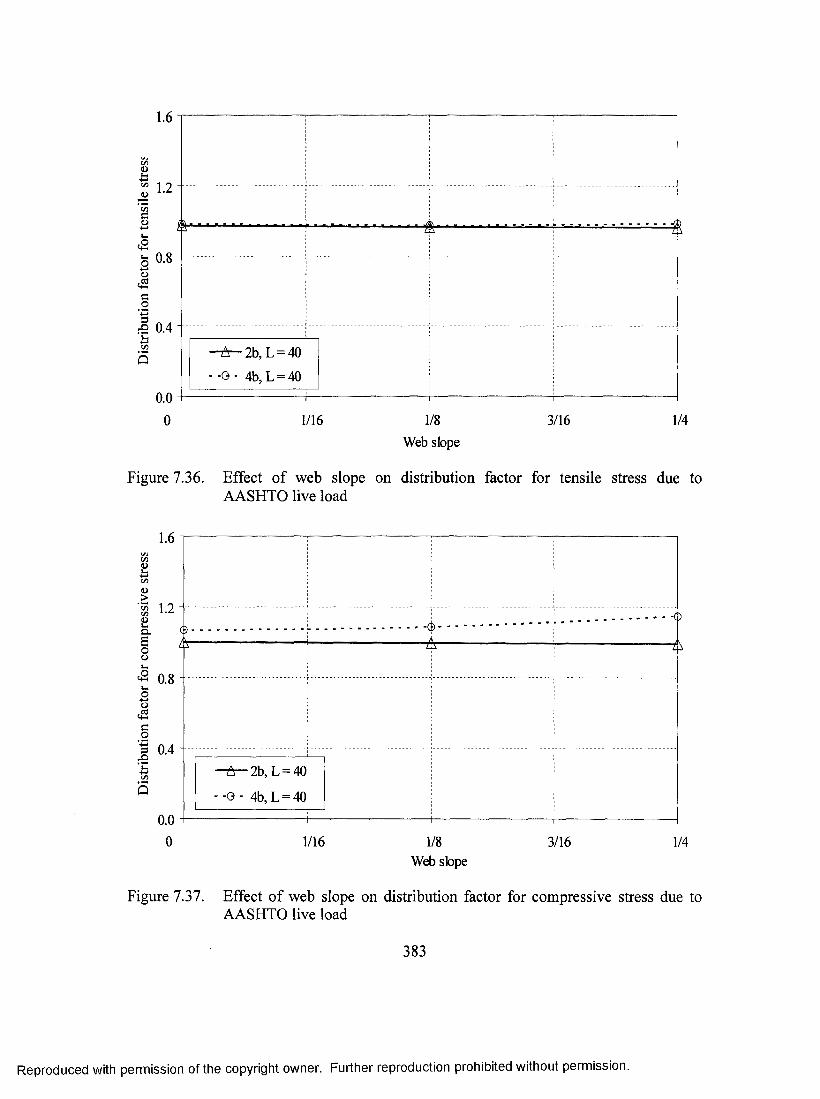
1.6
c/5O1.2
c
c20.8
o
o
I 0.4
0.0
1.6c/3Uhc/3
<U>1.2
o.eoo.2
o.'ciCo
«-Z!r
0.8
sj=
Q
0.4
0.0
-A -2b,L = 40 -O- 4b,L = 40
■ii
1/16 1/8 Web slope
3/16 1/4
Figure 7.36. Effect of web slope on distribution factor for tensile stress due to AASHTO live load
-T ^2b ,L = 40
- G - 4b,L = 40
■o
1/16 1/8 Web sfope
3/16 1/4
Figure 7.37. Effect of web slope on distribution factor for compressive stress due to AASHTO live load
383
Reproduced with permission of the copyright owner. Further reproduction prohibited without permission.

1.6
i 1.2u
T3,P
So
0.8
t/)5
0.4
0.0
^ ?s-2b ,L = 40
- -0 - 4b,L = 40
Figure 7.38.
1/16 1/8 Web slope
3/16 1/4
Effect of web slope on distribution factor for deflection due to AASHTO live load
1.6
( 3 -
O
od_o3
/It1.2-
0.8
5 0.4
0.0
<?-
- A - N b = 2,L = 40
- - 0 - Nb = 4,L = 40
<)
1/16 1/8 Web sbpe
3/16 1/4
Figure 7.39. Effect of web slope on distribution factor for shear force due to AASHTO live load
384
Reproduced with permission of the copyright owner. Further reproduction prohibited without permission.

1.6co
tia§■o■C(D
( 5 -
Z!r1.2
“ 0.8
o,cdC.2"3X)•£
0.4 -
0.0
-75r-2b,L = 40
-O- 4b,L = 40
<)
1/16 1/8 Web slope
3/16 1/4
Figure 7.40. Effect of web slope on distribution factor for exterior support reaction due to AASHTO live load
„ 1.6 _o1-do 1 2a,3t/5
Z ! r
0.8
o, 3<+H3_o'3JD
0.4 -
t/3
50.0
e-
-75r-2b,L = 40
-0 - 4b,L = 40
o
■tI\
1/16 1/8 Web slope
3/16 1/4
Figure 7.41. Effect of web slope on distribution factor for interior support reaction due to AASHTO live load
385
Reproduced with permission of the copyright owner. Further reproduction prohibited without permission.
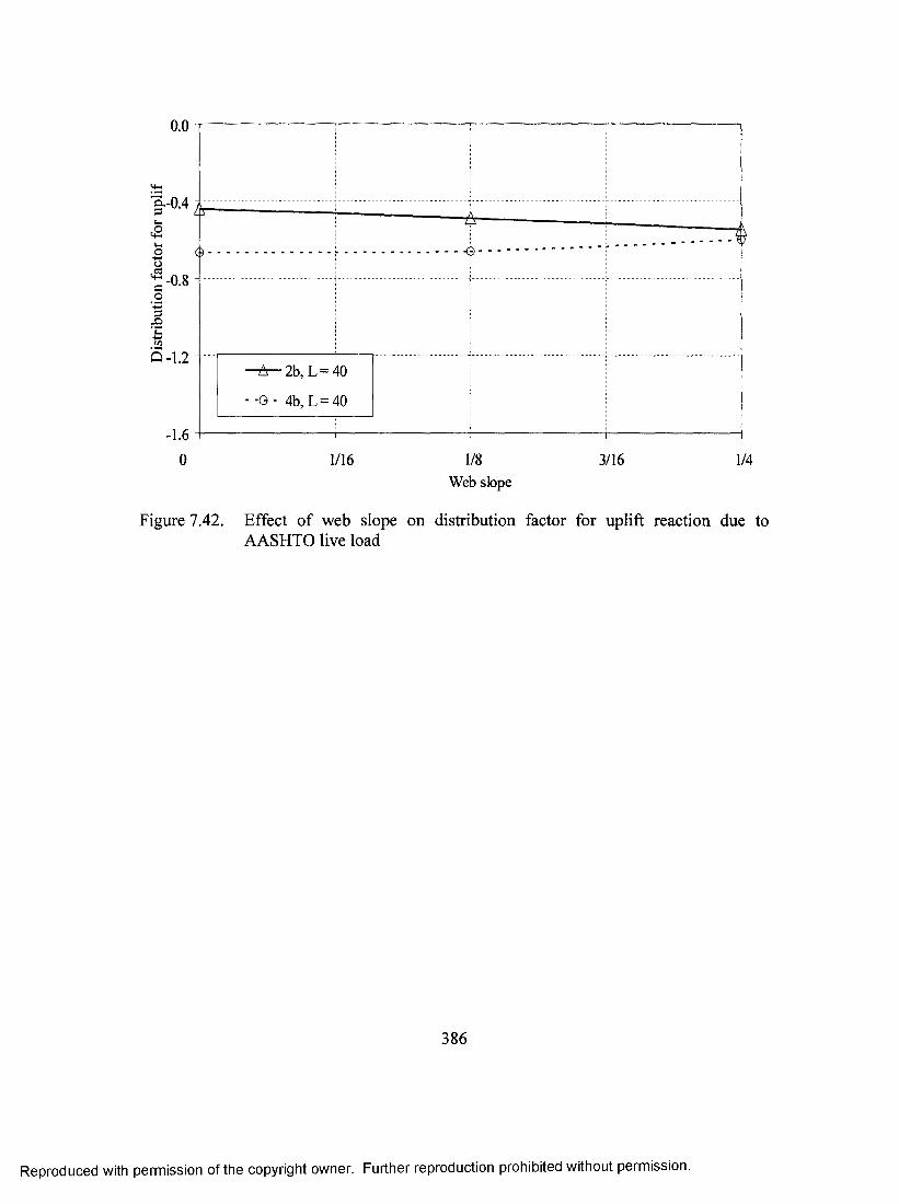
0.0
B.-0.4
5-1.2
-1.60 1/16 1/8 3/16 1/4
Web slope
Figure 7.42. Effect of web slope on distribution factor for uplift reaction due to AASHTO live load
386
Reproduced with permission of the copyright owner. Further reproduction prohibited without permission.

3.0
onS2.5WC/5g 2.0■4-JUi<22 1.5
1.0
t*-!Co
x>1n 0.5
0.0
L/R =0.0 -0- -L/R= 1.2
>0
Figure 7.43.
3.0
20 25Span-to-depth ratio
Effect of span-to-depth ratio on distribution factor for tensile stress
onc/5
u 2.5 .S:*75
c/5
§■2.0B
l u
tw Ci .2 "3
iQ
1.0
0.5
0.0
—)I0--L/R = 0.0_ 0 _ •L/R = 1.2
5 -
20 25
30
i )
30Span-to-depth ratio
Figure 7.44. Effect of span-to-depth ratio on distribution factor for compressive stress
387
Reproduced with permission of the copyright owner. Further reproduction prohibited without permission.
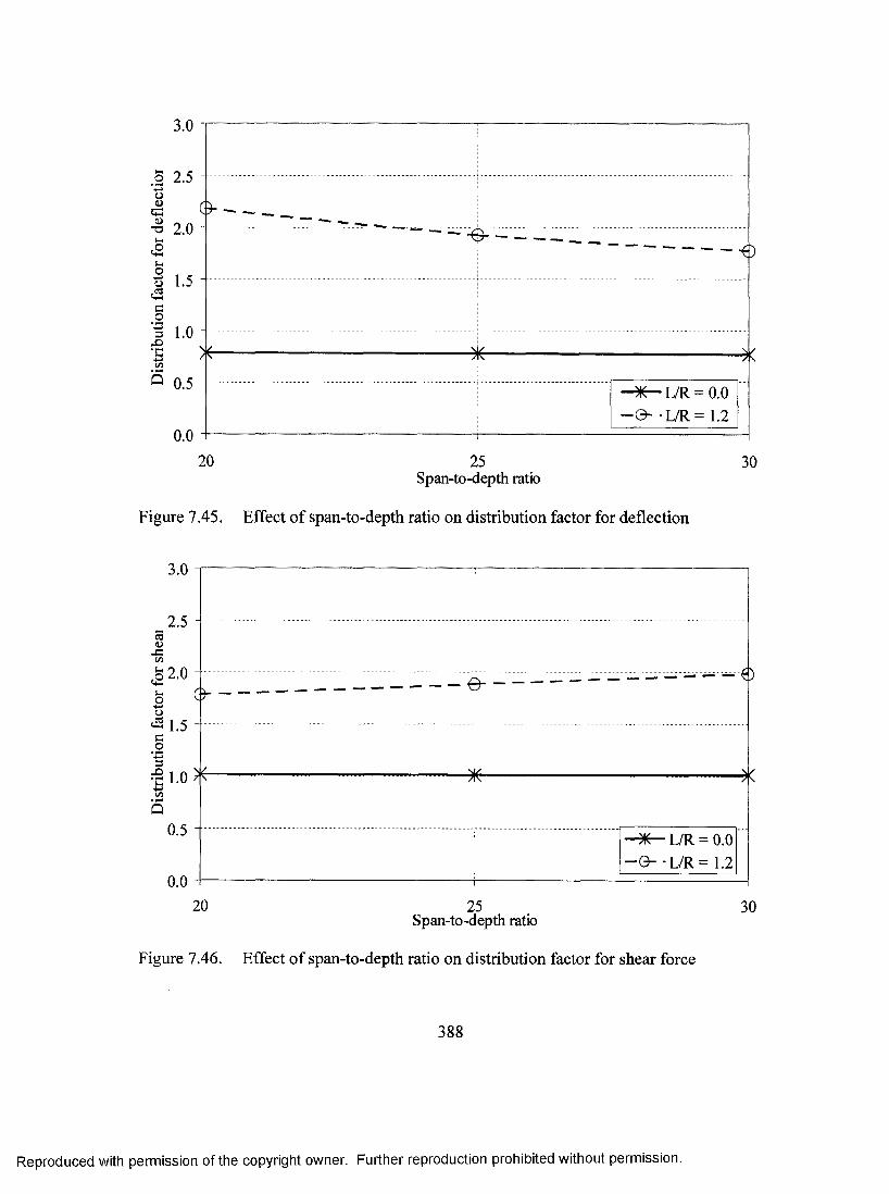
3.0
.2 2.5ouC
-O 2.0
ooco
1.5
3 1. JD 1.0
Q 0.5 -
0.020 25
- ^ L / R = 0.0 -0- -L/R= 1.2
30Span-to-depth ratio
Figure 7.45. Effect of span-to-depth ratio on distribution factor for deflection
3.0
2.5
12.0 -O-
43 1.5co3X)c 1.0C/5
Q0.5 -
0.020
e -
25
L/R = 0.0 -0- -L/R= 1.2
Span-to-depth ratio
Figure 7.46. Effect of span-to-depth ratio on distribution factor for shear force
30
388
Reproduced with permission of the copyright owner. Further reproduction prohibited without permission.
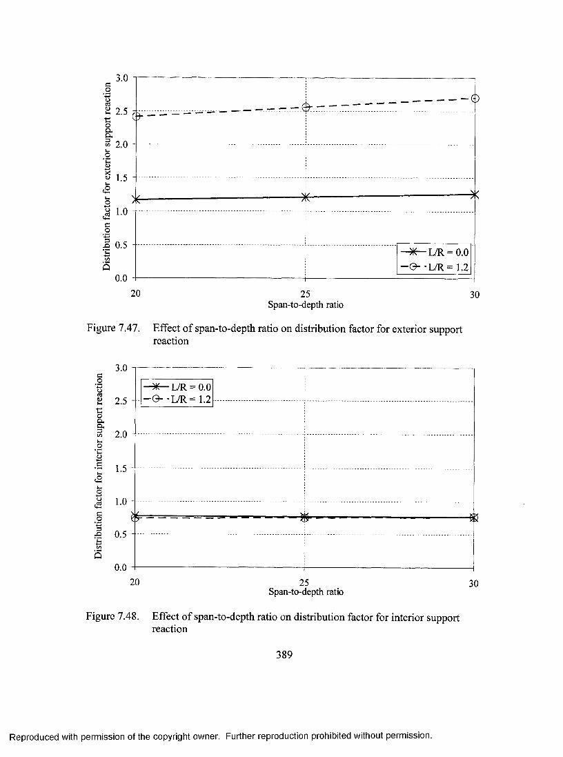
_o
(Uu<t;oD<O.
3.0
2.5 (>-
2.0.2><w
k.1oo,tdu-ia.2"3
1.5
1.0
0.5 -
0.020
■0
25Span-to-depth ratio
■ ^ L /R = 0.0 -0- -L/R= 1.2
30
Figure 7.47. Effect of span-to-depth ratio on distribution factor for exterior support reaction
c_o
■daat/j
o,c<3
Co
3.0
2.5
2.0
1.5
1.0
2 0.5
0.0
-L/R = 0.0_ 0 _ ■L/R = 1.2
20 25Span-to-depth ratio
30
Figure 7.48. Effect of span-to-depth ratio on distribution factor for interior supportreaction
389
Reproduced with permission of the copyright owner. Further reproduction prohibited without permission.

0.0
-0.5>(-
Cl.3<2 -1-UO'o
1.0 -
« -1.5 -aoZ3
*cc -2.0
-2.5 -
-3.0
■€)
L/R = 0.0 '©■ -L/R= 1.2
20 25 30Span-to-depth ratio
Figure 7.49. Effect of span-to-depth ratio on distribution factor for uplift reaction
390
Reproduced with permission of the copyright owner. Further reproduction prohibited without permission.

C3O
o<4HC_o'+33-E00
5
2.0
—♦— Internal & external bracing (live load)- - Internal bracing (live load)—X — Internal & external bracing (dead load) —0 ■ ■ Internal bracing (dead toad)
1.8
1.6
1.4
1.2
1.0
1 3 5 97 IINumber o f cross bracings
Figure 7.50. Effect of number of bracings on distribution factor for tensile stress
t/i
>
&eoO
oC.2
.3
2.0—♦— Intemal & external bracing (live toad)- -A - Intemal bracing (live toad)—X — Intemal & extemal bracing (dead toad) —0 ■ ■ Intemal bracing (dead toad)
1.8
1.6
1.4
1.2
1.0
3 5 7 91 11Number o f cross bracings
Figure 7.51. Effect of number of bracings on distribution factor for compressive stress
391
Reproduced with permission of the copyright owner. Further reproduction prohibited without permission.
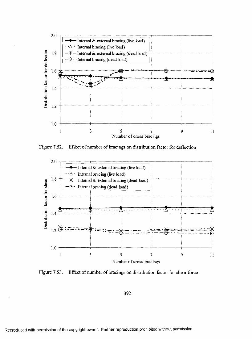
o(UGa>
<22
e_o"3'200
5
2.0
1.8 -
1.6
L\
1.4
1.2
1.0
—♦— Intemal & extemal bracing (live load)- -A - Intemal bracing (live load)—X — Intemal & extemal bracing (dead load) “ 0 - ■ Intemal bracing (dead load)
'A ’
1 5 7Number of cross bracings
11
Figure 7.52. Effect of number of bracings on distribution factor for deflection
2.0
a 1.8C/3U2
o
ao
1.6
S 1.43X>'B(5
1.2
1.0 4
..♦ ...Intemal & extemal bracing (live load)" -A - Intemal bracing (live load)—X — Intemal & extemal bracing (dead load) —0 ■ ' Intemal bracing (dead load)
-------- 4 ..—.....” .................... & ......................5 ....................... ------A ........... .................... -A
_N/-..... ..........---*5
-------------------- --------------------------------------
---------------- 0
1 3 5 7 9Number of cross bracings
Figure 7.53. Effect of number of bracings on distribution factor for shear force
11
392
Reproduced with permission of the copyright owner. Further reproduction prohibited without permission.
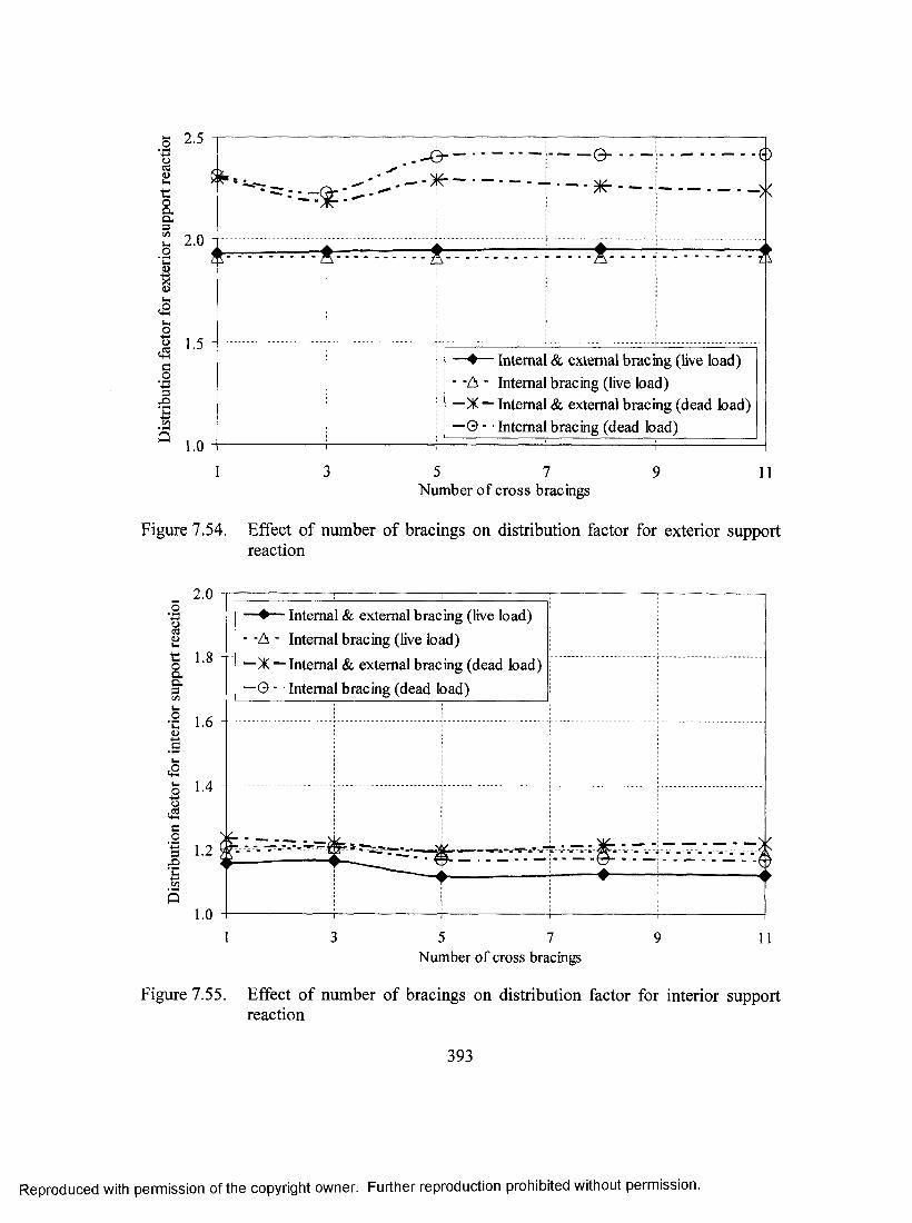
.2
■coa.O h
.2'Cu><u
C.2p43MQ
2.0
1.5
1.0
- t -
-e - 0
><
................
-♦— Intemal & extemal bracing (live load) -A - Intemal bracing (live load)■X — Intemal & extemal bracing (dead load) ■0 - ■ Intemal bracing (dead load)
5 7Number of cross bracings
9 1 1
Figure 7.54. Effect of number of bracings on distribution factor for exterior support reaction
2.0
C3
ut:oaa.=3c/5UO*CoU4
o,SJc_2"SXi'B
1.8 -
1.6
1.4
1.2
1.0
Figure 7.55.
—♦— Intemal & extemal bracing (live load)- -A - Intemal bracing (live load)—X — Intemal & extemal bracing (dead load) —0 - ■ Intemal bracing (dead load)
^----^/------
..
▲
..................... .
r
-...... ...... . ... . “ ...... ..... ■■5 7
Number of cross bracings11
Effect of number of bracings on distribution factor for interior support reaction
393
Reproduced with permission of the copyright owner. Further reproduction prohibited without permission.
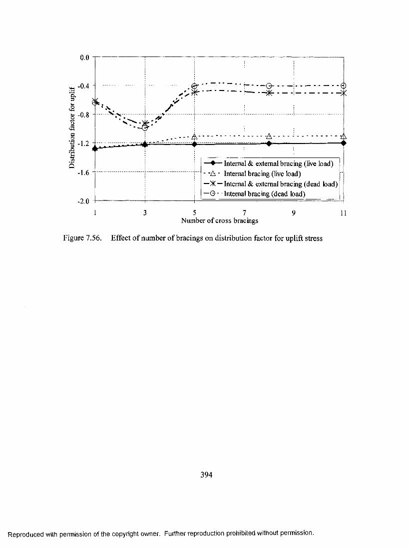
-0.4a.3U
3O3
i/j5
- 0.8
- 1.2
- 1.6
- 2.0
Intemal & extemal bracing (live load)- -A ■ Intemal bracing (live load)—X — Intemal & external bracing (dead load) —G - ■ Intemal bracing (dead load)
5 7Number of cross bracings
1 1
Figure 7.56. Effect of number of bracings on distribution factor for uplift stress
394
Reproduced with permission of the copyright owner. Further reproduction prohibited without permission.

73CD■oOQ .coCDQ .
■DCD
C/)
o'oo
oo■D AASHTO LRFD17.5 72.5 72.5
HS20-441 ^ 4 , «in
WHEEL LOADS, kN
3CD
CP-
55 55 WHEEL Design Tandem __ , LOADS, kN
1.2m
CD■oOQ .Cao=5
■oo
CDQ.
U)
CL-625 25 62.5 62.5 87.5WHEEL
-— 3.6m — 1.2m . m . Ill
oc■oCD
C/)
o'13
CL-625-ONT 25 70 70 87.5 60
3.6m — .u ii . m . m
WHEEL LOADS, kN
Figure 7.57. Truck loading considered in AASHTO LRFD and CHBDC codes

3.0—©— AASHTO - -A ■ AASHTO LRFD
- CL-625 -X-CL-625-ONT
I 2.5 -
2.0 -C3B
o<4-1
co3bQ 0.5
0.0 H-----Bridge 1 Bridge 2 Bridge 3
Figure 7.58. Effect of truck loading specified in different codes on distribution factor for tensile stress
3.0—9— AASHTO - -A - AASHTO LRFD
CD625 -X -C D 625-O N T
O fl
1.0
Bridge 1 Bridge 2 Bridge 3
Figure 7.59. Effect of truck loading specified in different codes on distribution factor for compressive stress
396
Reproduced with permission of the copyright owner. Further reproduction prohibited without permission.

3.0
—e— AASHTO - -A - AASHTO LRFD
- CL-625 -X-CL-625-ONT
-S 2.0
0.5
0.0 ^—
Bridge 1 Bridge 2 Bridge 3
Figure 7.60. Effect of truck loading specified in different codes on distribution factor for deflection
3.0- e — AASHTO - -A - AASHTO LRFD
- CL-625 - X - CL-625-ONT
2.5
oo,sSco
Q0.5
0.0 i -----
Bridge 1 Bridge 2 Bridge 3
Figure 7.61. Effect of truck loading specified in different codes on distribution factor for shear force
397
Reproduced with permission of the copyright owner. Further reproduction prohibited without permission.
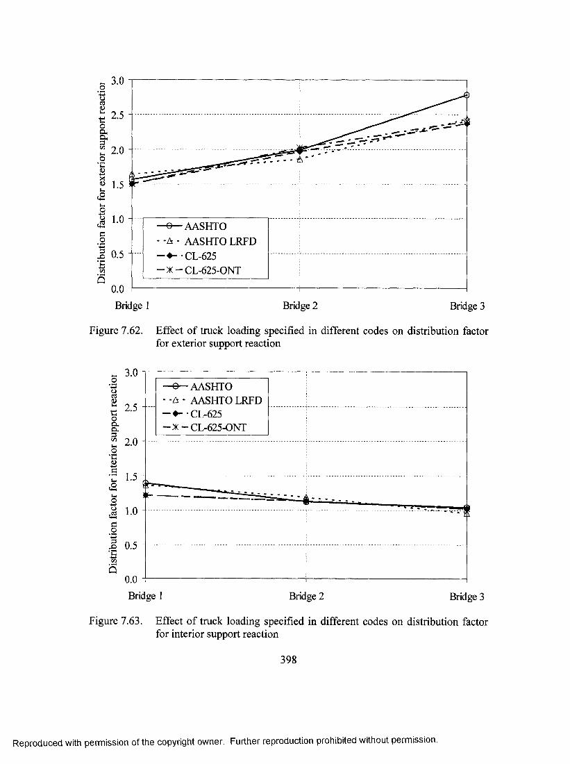
o
2.0
a—e —AASHTO - -A - AASHTO LRFD
CL-625 -X-CL-625-ONT
3 0.5
0.0 —
Bridge 1 Bridge 2 Bridge 3
Figure 7.62. Effect of truck loading specified in different codes on distribution factor for exterior support reaction
« 3.0Oa 2.5 - -
-e-AASHTO -A - AASHTO LRFD
■CL-625 -X-CL-625-ONT
Bridge 1
Figure 7.63.
Bridge 2 Bridge 3
Effect of truck loading specified in different codes on distribution factor for interior support reaction
398
Reproduced with permission of the copyright owner. Further reproduction prohibited without permission.
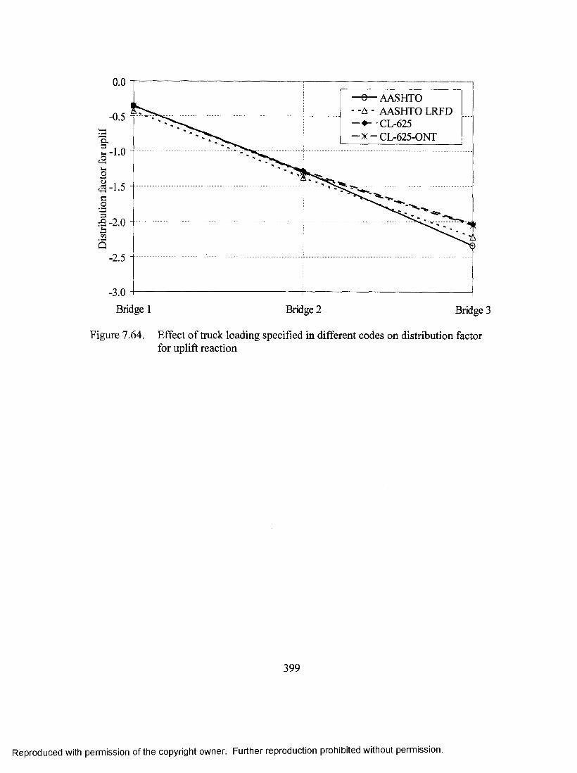
0.0—e— AASHTO - - A - AASHTO LRFD
CL-625 -X-CL-625-ONT
-0.5 - -
-2.5
-3.0 H-----Bridge 1 Bridge 2 Bridge 3
Figure 7.64. Effect of truck loading specified in different codes on distribution factor for uplift reaction
399
Reproduced with permission of the copyright owner. Further reproduction prohibited without permission.
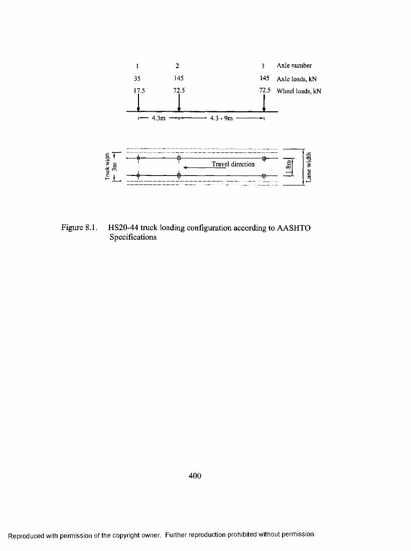
1
35
17,5
2
145
72.5
4.3m 4.3 - 9m
3 Axle number
145 Axle loads, kN
72.5 Wheel loads, kN
3 1 •— 4--------------- i i — E Travel direction S
___________ i:________^____ ~
€
gi-i
Figure 8.1. HS20-44 truck loading configuration according to AASHTO Specifications
400
Reproduced with permission of the copyright owner. Further reproduction prohibited without permission.

R I 1 .
Fc
UPj2 I P|2
Figure 8.2. Vehicle idealization
R
(P /2 fl.l7 F c) (P/2+1.17 Fc)
lFc/2
Wheel load and centrifugal force Equivalent forces at centre of the concerte deck
401
Reproduced with permission of the copyright owner. Further reproduction prohibited without permission.

a)
R = 5 0 m
One-loaded lane
R = 50 m------------------------►1
................... ^n -
1
Two-loaded lane
R = 50 m
Three-loaded lane
R = 50 m
Four-loaded lane
b)
10m Travel direction, v = 50 km/h
20m 20m
Figure 8.3. Loading locations considered in: a) trasverse direction; and b) longitudinal direction
402
Reproduced with permission of the copyright owner. Further reproduction prohibited without permission.
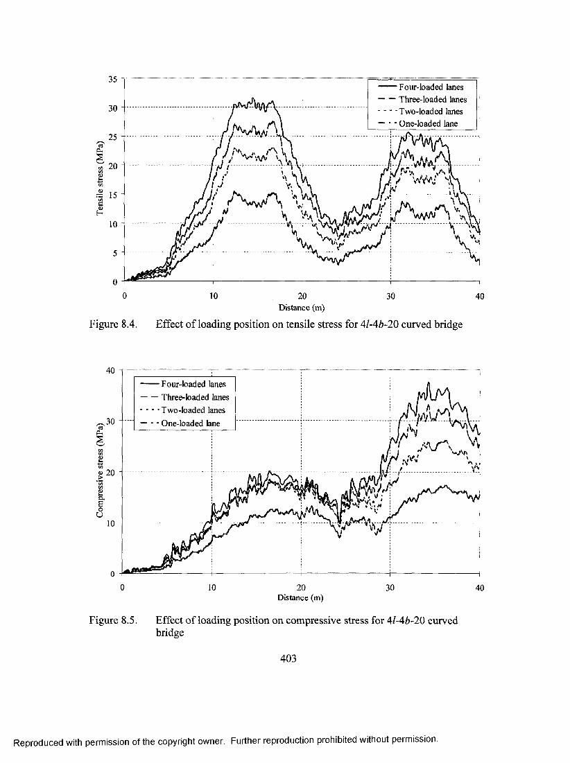
Four-loaded lanes Three-loaded lanes Two-loaded lanes One-loaded lane
Figure 8.4.
10 3020Distance (m)
Effect of loading position on tensile stress for 4l-4b-20 curved bridge
40
40 Four-loaded lanes Three-loaded lanes- ■ ■ - Two-loaded lanes— - - One-loaded lane
II 20
aQ.EoO
10
010 20
Distance (m)30 40
Figure 8.5. Effect of loading position on compressive stress for 4/-46-20 curved bridge
403
Reproduced with permission of the copyright owner. Further reproduction prohibited without permission.
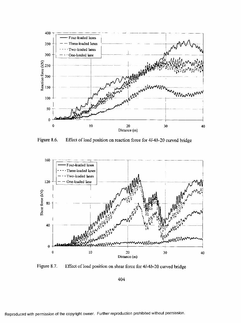
F o u r - l o a d e d la n e s T h r e e - l o a d e d la n e s T w o - l o a d e d la n e s O n e - l o a d e d la n e
- A * -I V - - - -Jt I -)ir .250
I 150 Qd
10 20D i s t a n c e ( m )
30 40
Figure 8.6. Effect of load position on reaction force for 4/-4Z>-20 curved bridge
F o u r - l o a d e d la n e s ■ ■ - T h r e e - l o a d e d la n e s
— - - T w o - l o a d e d la n e s — O n e - l o a d e d la n e
5 80V( .
. >V .1'' ,\ It
' a;-:'' ^ft'
10 20D i s t a n c e ( m )
30 40
Figure 8.7. Effect of load position on shear force for 4/-46-20 curved bridge
404
Reproducecl with permission of the copyright owner. Further reproduction prohibited without permission.

(S
e<u
30
V = 60 km/h V= 100 km/h V= 140 km/h
25
15
10\j
5
0150 10 20 255 30 35 40
Figure 8.8.
Distance (m)
Effect of vehicle speed on tensile stress for 4/-66-20 straight bridge
<ufc
£a.EoU
40 V = 60 km/h- - - -V =100 km/h V =140 km/h
30
20
10
00 105 15 20 25 30 35 40
Distance (m)
Figure 8.9. Effect of vehicle speed on compressive stress for 4l-6b-20 straight bridge
405
Reproduced with permission of the copyright owner. Further reproduction prohibited without permission.
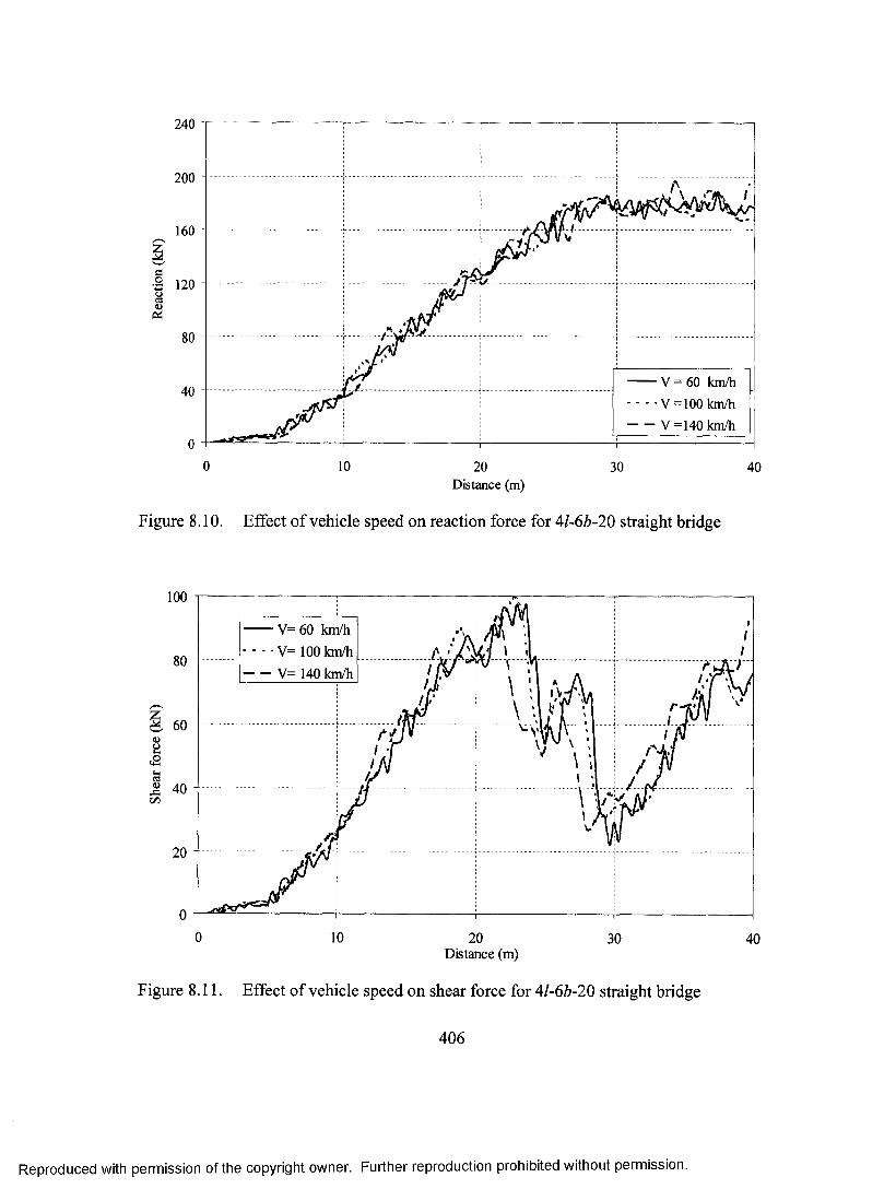
240
200 -
160 -I ^ 120 -
80 -
V = 60 km/h V =100 km/h V =140 km/h
40 -
0 10 20 30 40Distance (m)
Figure 8.10. Effect of vehicle speed on reaction force for 4l-6b-20 straight bridge
100
- V= 60 km/h- -V= 100 km/h- V= 140 km/h
§
0 10 20 30 40Distance (m)
Figure 8.11. Effect of vehicle speed on shear force for 4l-6b-20 straight bridge
406
Reproduced with permission of the copyright owner. Further reproduction prohibited without permission.

eSOi
U
c<L>H
32
DIRECT 50 MODES 100 MODES 200 MODES
24
16
8
0
80 10 20 30 40
Distance (m)
Figure 8.12. Comparison between direct integration and superposition methods for tensile stress of 2l-2b-20 straight bridge
16 DIRECT 50 MODES 100 MODES 200 MODES12
8
4
0
COCLhS
I<u>a .6oU
10 20Distance (m)
30 40
Figure 8.13. Comparison between direct integration and superposition methods for compressive stress of 2l-2b-20 straight bridge
407
Reproduced with permission of the copyright owner. Further reproduction prohibited without permission.

ac_o1
220— D I R E C T— 5 0 M O D E S- - 1 0 0 M O D E S- - 2 0 0 M O D E S
1 8 0
1 4 0
100
6 0
20
-200 10 20 3 0 4 0
D i s t a n c e ( m )
Figure 8.14. Comparison between direct integration and superposition methods for reaction force of 2l-2b-20 straight bridge
1 4 0— D I R E C T— 5 0 M O D E S- ■ 1 0 0 M O D E S- - 2 0 0 M O D E S
120 -
100 -
8 0 -O
S 6 0 -uJSon
4 0 -
20 -
0 10 20 3 0 4 0D i s t a n c e ( m )
Figure 8.15. Comparison between direct integration and superposition methods for shear force of 2l-2b-20 straight bridge
408
Reproduced with permission of the copyright owner. Further reproduction prohibited without permission.

c<u
30
25
20
15
10At =0.002 At =0.010At =0.015 At =0.020
5
00 10 3020
Distance (m)
Figure 8.16. Effect of time step on tensile stress of 2/-2Z>-20 curved bridge
40
At =0.002 At =0.010 At =0.015 At =0.020
0 10 3 020Distance (m)
Figure 8.17. Effect of time step on compressive stress of 2l-2b-20 curved bridge
4 0
409
Reproduced with permission of the copyright owner. Further reproduction prohibited without permission.
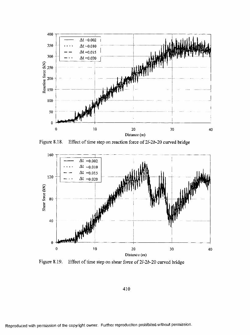
400At =0.002 At =0.010 At =0.015 At =0.020
350
300
Uo200
o
100
0 10 20 30 40Distance (m)
Figure 8.18. Effect of time step on reaction force of 2l-2b-20 curved bridge
160At =0.002 At =0.010 At =0.015 At =0.020120 - -
<a80 -
40 -
0 10 20 30 40
Figure 8.19.Distance (m)
Effect of time step on shear force of 2l-2b-20 curved bridge
410
Reproducecl with permission of the copyright owner. Further reproduction prohibited without permission.

s
c(U
35At =0.005
30At =0.020
25
20
15
10
5
0
Figure 8.20.
20 40 80 10060Distance (m)
Effect of time step on tensile stress of 3l-3b-60 curved bridge
120
BO
cdCL.s
><ua
0
35At =0.005 At =0.014 At =0.020
30
25
15
10
5
020 40 80 10060
Distance (m)
Figure 8.21. Effect of time step on compressive stress of 3l-3b-60 curved bridge
120
411
Reproduced with permission of the copyright owner. Further reproduction prohibited without permission.
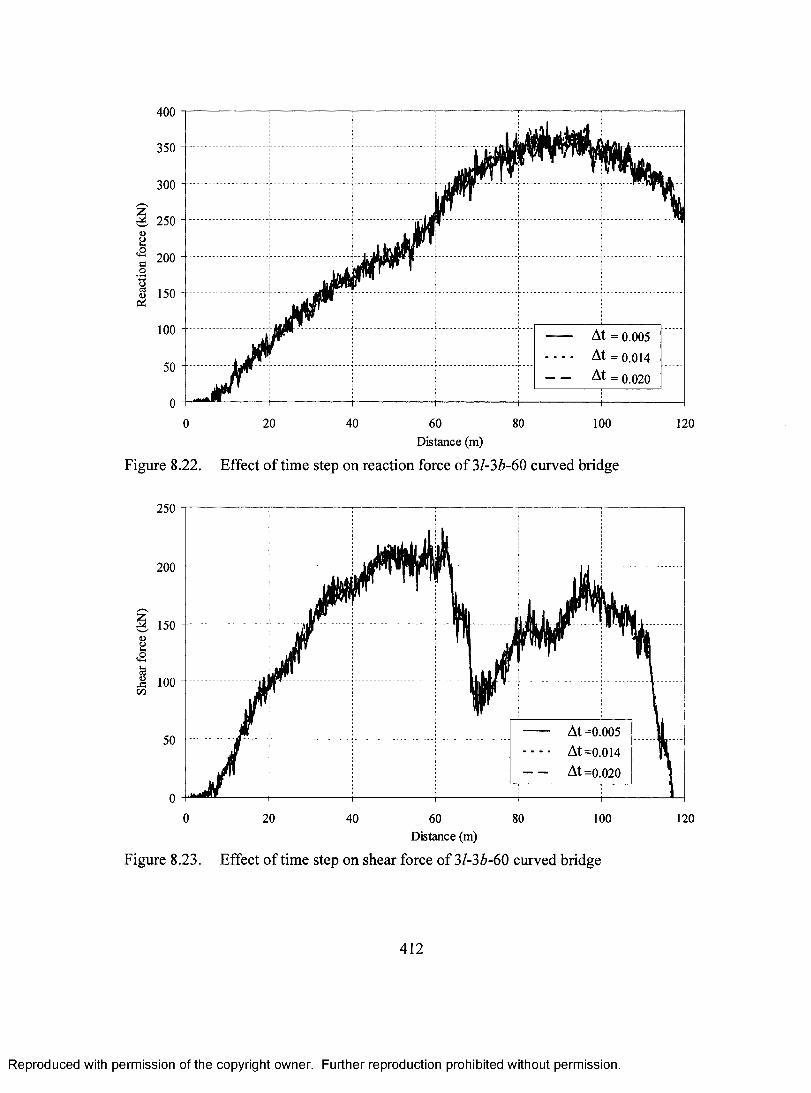
400
350 -
300 -
250 -o
200 -coS 150 - oi
100 - At = 0.005
50 -= 0.020
0 -H 0 20 40 60 80 100 120
Distance (m)
Figure 8.22. Effect of time step on reaction force of 3/-36-60 curved bridge
lUJ=(/2
0 20 40 8060Distance (m)
Figure 8.23. Effect of time step on shear force of 3l-3b-60 curved bridge
100
250
200
150
100
— At =0.005-• At =0.014- At =0.020
50
0120
412
Reproduced with permission of the copyright owner. Further reproduction prohibited without permission.
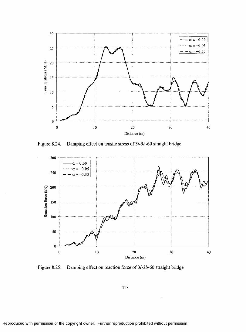
CO
wdJC<D
30
a = 0.00- - - - a = -0.05 a = -0.3325
15
10
5
02010 30 400
Distance (m)
Figure 8.24. Damping effect on tensile stress of 3l-3b-60 straight bridge
Distance (m)
Figure 8.25. Damping effect on reaction force of 31-3b-60 straight bridge
413
300 a = 0.00- - - - a = -0.05 a = -0.33250
I 200
d>o<s 150cot3
20 3010 400
Reproduced with permission of the copyright owner. Further reproduction prohibited without permission.

cflI
eu
o .s
12
— L/R=0.0 --e - L/R=0.1 - - L/R=0.2-A-L/R=0.4
10
8
6
4
232 4
N u m b e r o f la n e s
Figure 8.26. Effect of number of lanes on impact factor for tensile stress for 46-20 bridges
<D
C
Cu
10
8
6
4
-A--— L/R=0.0 - 0 - L/R=0.1 - -X - L/R=0.2 -A-L/R=0.4
2
032 4
N u m b e r o f b o x e s
Figure 8.27. Effect of number of boxes on impact factor for tensile stress for 46-20 bridges
414
Reproduced with permission of the copyright owner. Further reproduction prohibited without permission.

(1>
aa>
tjC3£Xe
8
— L/R=0.0 -><- -L/R=0.4
6
4
2
—-------0
20 40 60 80 100Span length (m)
Figure 8.28. Effect of span length on impact factor for tensile stress for 2l-2b bridges
hMcB
Ia.
10— 2l-2b-20 - > e -2l-2b-40
8
6
4
2>e
00.0 0.1 0.2 0 .3 0 . 4
Span-to-radius of curvature ratio (L/R)
Figure 8.29. Effect of span-to-radius of curvature ratio on impact factor for tensile stress for 2l-2b bridges
415
Reproduced with permission of the copyright owner. Further reproduction prohibited without permission.
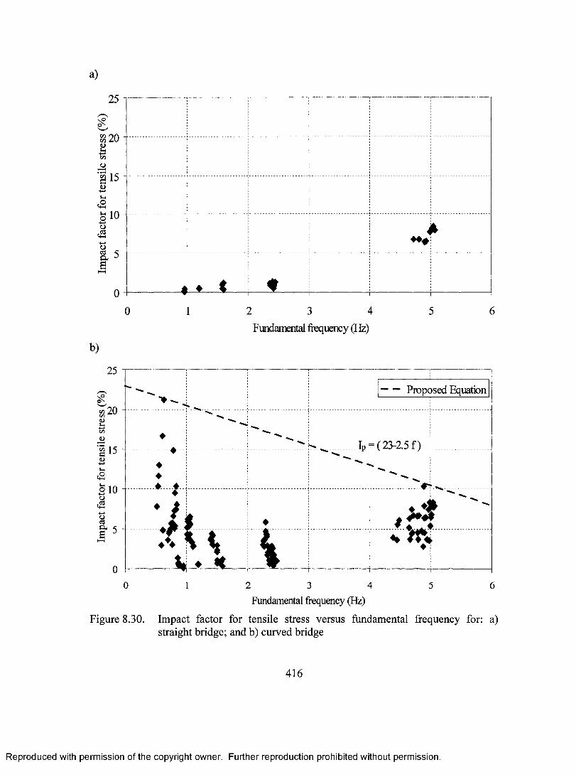
a)
3 4 60 1 2 5Fundamental frequency (Ffe)
b)
25
^20Vnto
15cj
olO
& 5
----- Proposed Equation
♦
...... ..........>>.
^ Ip = ( 23-2.5 f)♦♦♦
_____ ♦♦
1 ♦ W A . ♦
: vU
i ..................... ........................ i ................
Figure
0 1 2 3 4 5 6Fundamental frequency (Hz)
8.30. Impact factor for tensile stress versus fundamental frequency for: a) straight bridge; and b) curved bridge
416
Reproduced with permission of the copyright owner. Further reproduction prohibited without permission.
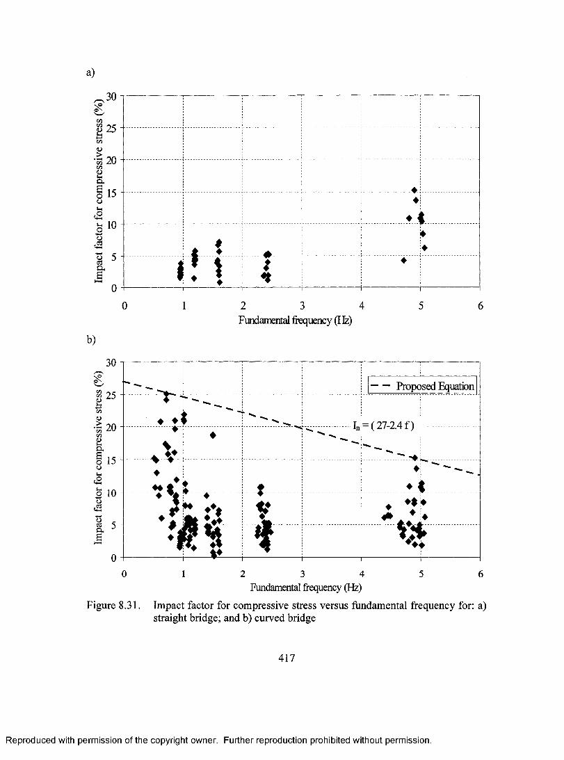
a)
Cl,
1 2 3 4 5 60Fundamental frequency (Hz)
b)
Proposed Equation
In = ( 27-2.4 f)
Figure 8.31.
1 2 3 4 5 6Fundamental frequency (Hz)
Impact factor for compressive stress versus fundamental frequency for: a) straight bridge; and b) curved bridge
417
Reproduced with permission of the copyright owner. Further reproduction prohibited without permission.
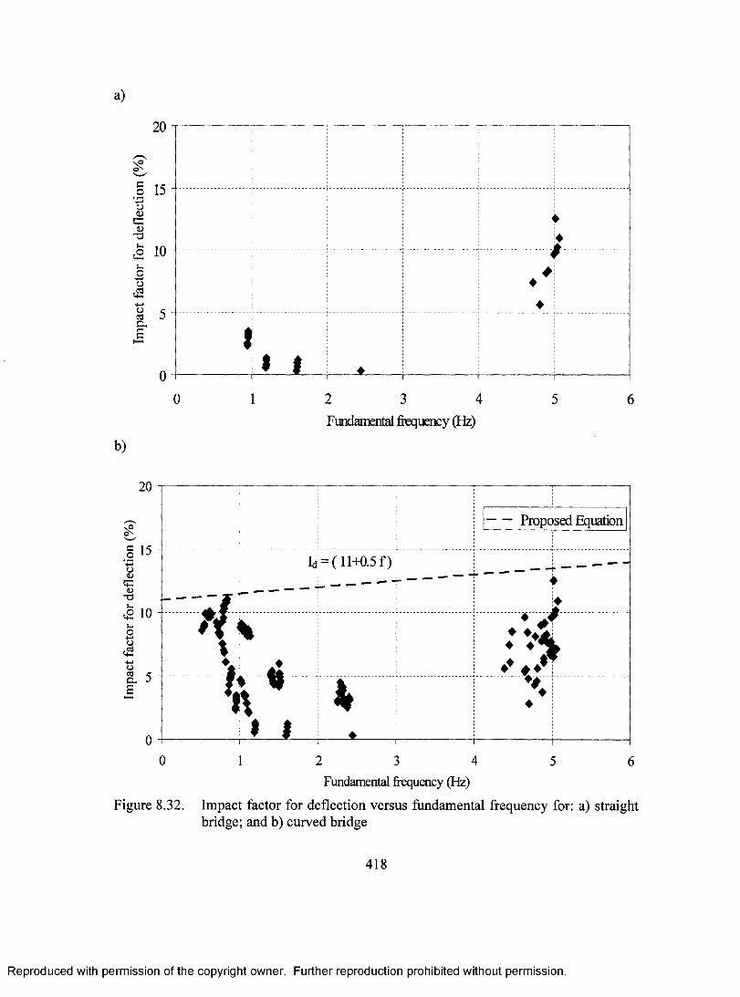
a)
C3_oo(DG0)
T3
c22o,C3f+H+->OcSD hB
20
15
10
5
01 2 3 40 5 6
Fundamental frequency (Hz)
b)
20
eI 15OCdj
^ 10 VhO•Mo
Qa- ^
00
Figure
----- Proposed Equation
Id = ( 11+0.5 f)------- --------- ►
♦*
....V%
.....4 ........
............ * 4 .*
♦♦ * /
F
< 1 ♦
♦
1 2 3 4 5 6Fundamental frequency (Hz)
8.32. Impact factor for deflection versus fundamental frequency for: a) straight bridge; and b) curved bridge
418
Reproduced with permission of the copyright owner. Further reproduction prohibited without permission.

a)
co20 -
^ 15 - o
10 -oC3as C -
0 1 2 3 4 65Fundamental frequency (Hz)
b)
30
25
o20c3
H ,o
0421Q,
15 -
10
-----Propo sed Equation
------------- Iro = (22-f )
..... .............A.
♦ --------------------
▼♦
♦
♦
♦ . ♦
............♦..AI *
1 \t*
i
n...................
♦♦ <
-------------- ' "0 1 2 3 4 5 6
Fundamental frequency (Hz)
Figure 8.33. Impact factor for exterior support reaction versus fundamental frequency for; a) straight bridge; and b) curved bridge
419
Reproduced with permission of the copyright owner. Further reproduction prohibited without permission.

a)
25 -
2 3 40 5 6Fundamental frequency (Hz)
b)
Proposed Equation
Iri = ( 18-0.5 f)
0 1 2 3 4 5 6Fundamental frequency (Hz)
Figure 8.34. Impact factor for interior support reaction versus fundamental frequency for: a) straight bridge; and b) curved bridge
420
Reproduced with permission of the copyright owner. Further reproduction prohibited without permission.

a)
200
120 -
63 4 50 1 2
b)
200
^160
IS 120
B^ 80 4-»ocd
40
Fundamental frequency (Hz)
♦
*
I u - ( 1 6 0 )
♦♦♦♦♦
s
Proposed Equation
- - V r -
i A
0 1 2 3 4 5Fundamental fiequency (Hz)
Figure 8.35. Impact factor for uplift reaction versus fundamental frequency for: a) straight bridge; and b) curved bridge
421
Reproduced with permission of the copyright owner. Further reproduction prohibited without permission.
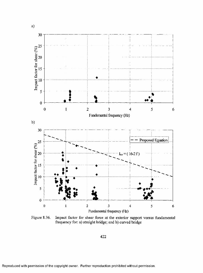
a)
HH
0 1 2 3 4 5 6Fundamental jfrequency (Hz)
b)
30
25s®
1 2 0kN,o
15o
J IOo,S
-----Proposed Equation
...................4..♦% ♦
. .. ^ .... ho ~ ( ][6-2 f )
" ......♦ ♦ ♦
♦
♦ ^ ^
n............ ♦ i - w . , ............ __ ♦ 1 . J r
" - ........... .^ -........... ...... " ......... ............... ................... - ..T“
Figure 8.36.
1 2 3 4 5 6Fundamental frequency (Tfe)
Impact factor for shear force at the exterior support versus fundamental frequency for; a) straight bridge; and b) curved bridge
422
Reproduced with permission of the copyright owner. Further reproduction prohibited without permission.

a)
u,aCO
40
30 -
20
0Cjo .1 10 ♦ ♦
t * }t
.............. %
%
2 3 4Fundamental frequency (Hz)
b)
40
ao>C O
Oo,c3
30
20
uc3a.S 10
▲
----- Proposed Equation
wt i = (37-41
^
')
♦ ♦♦ ♦
♦.A ♦
♦
^♦♦
♦ . A
_
m ...................
♦ > 4
" 4.....................r '...............1 6
Figure 8.37.
2 3 4 5Fundamental frequency (Hz)
Impact factor for shear force at the interior support versus fundamental frequency for: a) straight bridge; and b) curved bridge
423
Reproduced with permission of the copyright owner. Further reproduction prohibited without permission.

a)
I 30-
I 20--Moaaal-H
10-
20 60 80 100 1200 40
b)
60
^ 5 0
u40‘mfl^3 0
J 2 0<4H
o1^10
Span length (m)
------ Proposed Equation- X - CHBDC2000 - -G- AASHTOLRFD -A -A A SH T O 1996 -•-A A S fir O 2 0 0 3
------------ ^-------- i----------------------
6 ------------ i -------------i
'"■'Z
_ _ _ 1 - - I 1 _________ !20 40 60 80
Span length (m)100 120
Figure 8.38. Impact factor for tensile stress versus span length for: a) straight bridge; and b) curved bridge
424
Reproduced with permission of the copyright owner. Further reproduction prohibited without permission.

a)
^ 50-
40 -1 /1CO
' r 20-
10 -
40 60 80 1000 20 120Span length (m)
b)
<U>COHC l.
oo
Bo
0C31
60
50
40
30
20
10
Proposed Equation- y K - CHBDC2000 - -O - AASHTOIEFD - A -AASHTO 19% - t - AASHTO 2003
r - r i n=( 25)-------------
20 40 60Span length (m)
80 100 120
Figure 8.39. Impact factor for compressive stress versus span length for; a) straight bridge; and b) curved bridge
425
Reproduced with permission of the copyright owner. Further reproduction prohibited without permission.
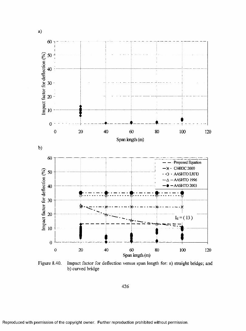
a)
T3
60 800 20 40 100 120
b)
60
40 -
a o*•+3 O(U0>
^ 30i-ioo5 20 o& 10
Span length (m)
------Proposed Equation-)K- CHBDC2000 - O - AASHTOLRFD - A - AASHTO 1996 - • - AASHTO 2003
1 - - - - - ■ ( I" #
! ----- ^e --------------) F-------------- ^ --------------k
*------ - _Id = (13)
1 ,--------------------^ ^ I f '
20 40 60 80Span length (m)
100 120
Figure 8.40. Impact factor for deflection versus span length for: a) straight bridge; and b) curved bridge
426
Reproduced with permission of the copyright owner. Further reproduction prohibited without permission.
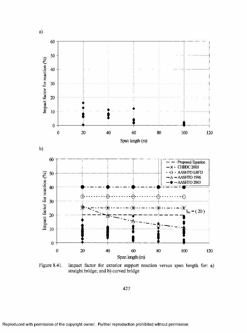
a)
50 -
do
oft's
10 -
200 40 60 80 100 120
Span length (m)
b)
60
50 - -
— ■ Proposed Equation )K- CHBDC2000 O ■ AASHTOLRFD A -AASHTO 1996 • -AASHTO 2003
« 30
Im -(2 0 )
20 40 60Span length (m)
80 100 120
Figure 8.41. Impact factor for exterior support reaction versus span length for: a) straight bridge; and b) curved bridge
427
Reproduced with permission of the copyright owner. Further reproduction prohibited without permission.
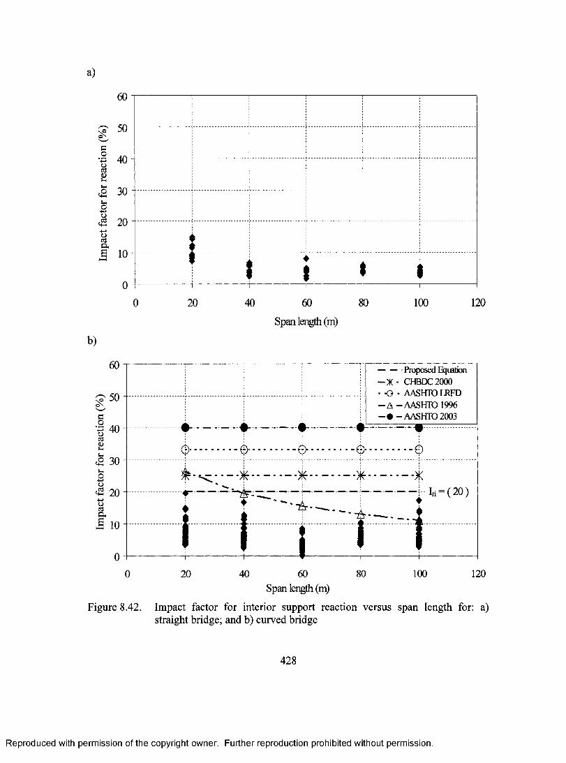
a)
ao40 -
30 -
20 -
10 -
80 100 1200 20 40 60
Span length (m)
b)
Proposed Equation X - CHBDC2000 -O - AASHTOLRFD A - AASHTO 1996
-AASHTO 2003 •
) r ■ ■ “ )lr ■ ■ ~ ---------------- )KIn = (20)20
20 40 60Span length (m)
80 100 120
Figure 8.42. Impact factor for interior support reaction versus span length for: a) straight bridge; and b) curved bridge
428
Reproduced with permission of the copyright owner. Further reproduction prohibited without permission.
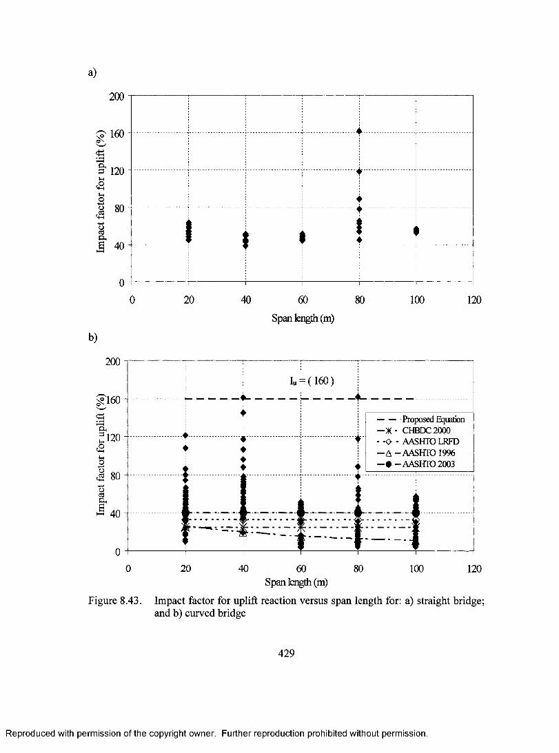
a)
200
160 -
80 -
20 40 600 80 100 120
b)
200
^160
120UcSuQi 80
40
Figure 8.43.
Span length (m)
Iu = (160)_♦---------
♦
♦
------ ■ Proposed Equation- X - CHBDC2000- -o ■AASHTOLRFD- A - ■AASHTO 1996
■AASHTO 2003
20 40 60Span length (m)
80 100 120
Impact factor for uplift reaction versus span length for: a) straight bridge; and b) curved bridge
429
Reproduced with permission of the copyright owner. Further reproduction prohibited without permission.
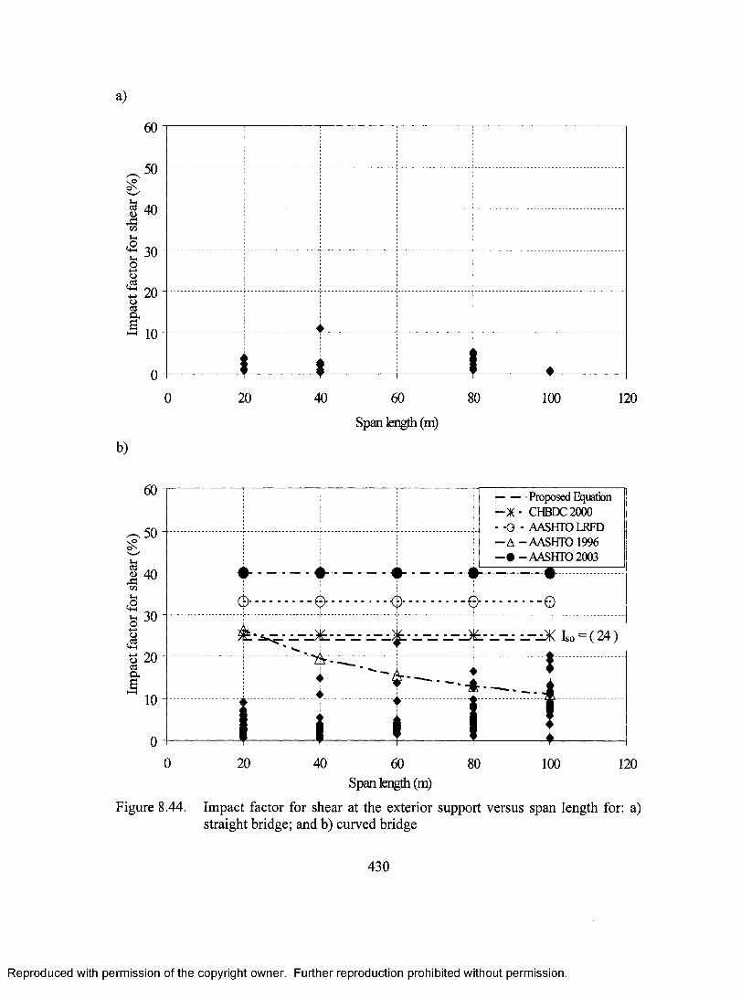
a)
g 40
20 40 60 800 100 120
Span length (m)
b)
60
50
| 4 0
01
30
> -
6--
- — ■ Proposed Equation -X- CHBDC2000 -O - AASHTO lEFD -A-AASHTO 1996 -•-AASHTO 2003
‘ ■ (S*.................. "(J)................ (i)
# - ............
Iso = ( 24 )
t ..................
♦
I___ i 1 !20 40 60
Span length (m)80 100 120
Figure 8.44. Impact factor for shear at the exterior support versus span length for: a) straight bridge; and b) curved bridge
430
Reproduced with permission of the copyright owner. Further reproduction prohibited without permission.

a)
50 -
^ 30 -u
20 -
10 -
0 20 40 60 80 100 120
Span length (m)
b)
60
50
c3C/a
Proposed Equation-)K - CHBDC2000 - -O - AASHTO U?FD - A -AASHTO 1996 - • -AASHTO 2003
- r ^ . T-. T-. T-. 7^ . r-. - - Isi ( 3 4 )
20 40 60Span length (m)
80 100 120
Figure 8.45. Impact factor for shear force at the interior support versus span length for: a) straight bridge; and b) curved bridge
431
Reproduced with permission of the copyright owner. Further reproduction prohibited without permission.
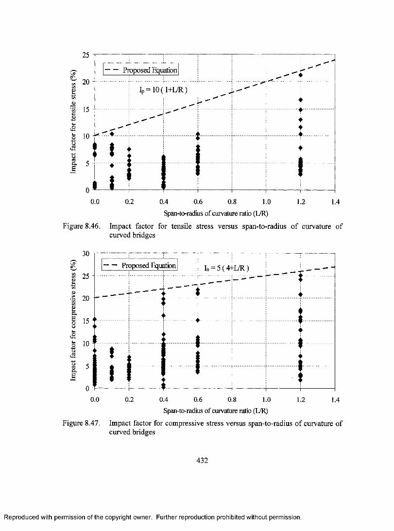
w1/3C /3
atoJi* c oCd>
<2o"S,<soc<3n.B
25
Proposed Equation20
15
10
5
00.0 0.2 0.4 0.6 0.8 1.0 1.2 1.4
Span-to-radius of curvature ratio (L/R)
Figure 8.46. Impact factor for tensile stress versus span-to-radius of curvature ofcurved bridges
s - /c/3C /3(DLn
30
25
C/3002o.ou
oo
ucs3O.
15
10II
-----Proposed Equation In-5(4HHL/R)— -4-
I
0 + - 0.0
I
t
♦
I♦
i
0.2 0.4 0.6 0.8 1.0
Span-to-radius of curvature ratio (L/R)1.2 1.4
Figure 8.47. Impact factor for compressive stress versus span-to-radius of curvature of curved bridges
432
Reproduced with permission of the copyright owner. Further reproduction prohibited without permission.
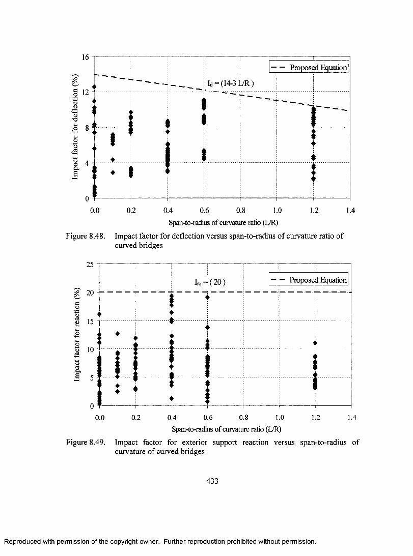
16
ou<D’OIH
O. a
^ 4 &
Proposed Equation
Id = (14-3iyR)
I♦
I♦
II
II
TI4
0.0 0.2 0.4 0.6 0.8 1.0Span-to-radius of curvature ratio (L/R)
1.2 1.4
Figure 8.48. Impact factor for deflection versus span-to-radius of curvature ratio of curved bridges
a.2csa
, o
o•4-»oaCl,
25
Proposed Equation20
15
10
5
00.80.0 0.2 0.4 0.6 1.0 1.2 1.4
Span-to-radius of curvature ratio (L/R)
Figure 8.49. Impact factor for exterior support reaction versus span-to-radius of curvature of curved bridges
433
Reproduced with permission of the copyright owner. Further reproduction prohibited without permission.

B
Ocd.1a
.2o<sCB
25
Proposed Equation
15
10
5
01.0 1.40.0 0.2 0.4 0.6 0.8 1.2
Span-to-radius of curvature ratio (LTR)
Figure 8.50. Impact factor for interior support reaction versus span-to-radius of curvature of curved bridges
'd-3u,o
o
200
150
100
ocdOdS 50
0
♦♦♦
♦
♦
0.0 0.2
♦♦
i 1 1 ■
Proposed Equation
Iu = (190-135L/R)
i1.2 1.40.4 0.6 0.8 1.0
Span-to-radius of curvature ratio (L/R)
Figure 8.51. Impact factor for uplift reaction versus span-to-radius of curvature of curved bridges
434
Reproduced with permission of the copyright owner. Further reproduction prohibited without permission.

NO
(/)u.2
O<13
D,
30
Proposed Equation25
20
15
10
5
00.0 0.2 1.2 1.40.4 0.6 0.8 1.0
Span-to-radius of curvature ratio (L/R)
Figure 8.52. Impact factor for shear force at the exterior support versus span-to-radius of curvature of curved bridges
cdOC/5Lh<2
O
oaCl
50
Proposed Equation40
30
20
10
00.4 0.6 0.8 1.0 1.20.0 0.2 1.4
Span-to-radius of curvature ratio (L/R)
Figure 8.53. Impact factor for shear force at the interior support versus span-to-radius of curvature of curved bridges
435
Reproduced with permission of the copyright owner. Further reproduction prohibited without permission.

a)
0 4020 60 80 100 120
b)
S p a n l e n g t h ( m )
3/-2 )-100,L/R = 0.6
Figure 9.1. Effect of bridge span length on: a) fundamental frequency; and b) mode shape
436
Reproduced with permission of the copyright owner. Further reproduction prohibited without permission.

a)
&&S=3cr0
1<Ds
§IX
5
4
□ L=20 m
- -A - L=60 m3
4b &L/R = 0.4
2
03 42
Number of lanes
0.774
0.731
2/-3/-80, L/R= 0.4 4l-3b-B0, L/R= 0.4
Figure 9.2. Effect of number of lanes on: a) fundamental frequency; and b) mode shape
437
Reproduced with permission of the copyright owner. Further reproduction prohibited without permission.
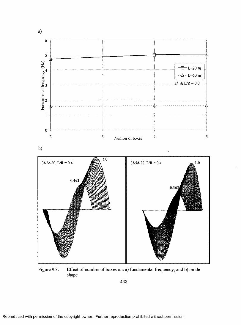
a)
NE^ 40 ag-< 3
1(D
-a-
-E h - L-20 m
--A- L=60 m
3/ &L/R = 0.0
A-
b)
Number of boxes ^
3/-2Z)-20, L/R = 0.4 3/-5Z)-20, L/R = 0.4
0.365
Figure 9.3. Effect of number of boxes on: a) fundamental frequency; and b) modeshape
438
Reproduced with permission of the copyright owner. Further reproduction prohibited without permission.
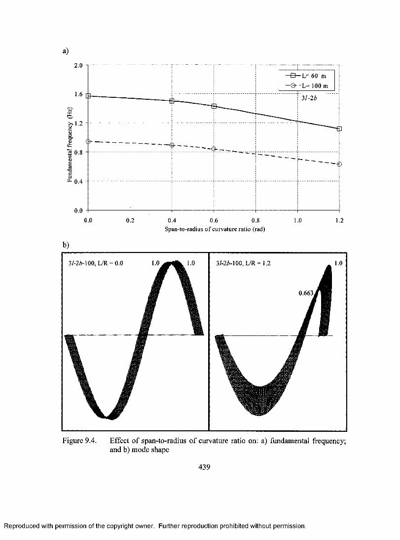
a)
2.0
■ S — L = 6 0 m 0 - - L = 1 0 0 m
2,1-2b
0 . 4
0.00.0 0.2 0 . 4 0.6 0.8 1.0 1.2
S p a n - t o - r a d i u s o f c u r v a t u r e r a t i o ( r a d )
b)
3 / - 2 6 - 1 0 0 , L / R = 0 . 0 3 / - 2 Z ) - 1 0 0 , L / R = 1 .2
0 . 6 6 3
Figure 9.4. Effect of span-to-radius of curvature ratio on: a) fundamental frequency; and b) mode shape
439
Reproduced with permission of the copyright owner. Further reproduction prohibited without permission.
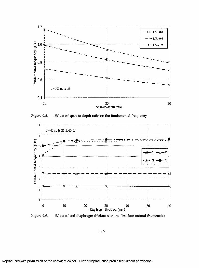
-□-■L/R=0.0
-O-L/R=0.6
-^-iyR=i.2
/= 100m,4/-36
20 25Span-to-depth ratio
30
Figure 9.5. Effect of span-to-depth ratio on the fundamental frequency
8
oc0O'
*
1 4(Ds•O Tc 33tlH
/=40iu 3/-26,L/R=0.4
" .- .“ ■.T.-J
[3-
)(-
i nTpr—
- ^ n - d -1 2
- A - o f4
E]
■3(
10 20 30 40DiafAragm thickness (mm)
50 60
Figure 9.6. Effect of end-diaphragm thickness on the first four natural frequencies
440
Reproduced with permission of the copyright owner. Further reproduction prohibited without permission.
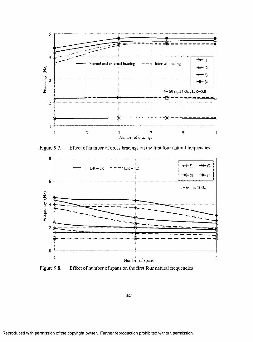
5
ss SB sa
4Internal and external bracing Internal bracing
3
/=60 m,3/-3Z>,L/R=0.8
2
3 5 7 9Number of bracings
Figure 9.7. Effect of number of cross bracings on the first four natural frequencies
8-S - f l -0 -f2
L/R = 0.0 L/R = 1.2
6L = 60m, 4Z-36
^ Ao 4
2
043
Number of spans2
Figure 9.8. Effect of number of spans on the first four natural frequencies
441
Reproduced with permission of the copyright owner. Further reproduction prohibited without permission.

X Fully-loaded lanes —B- • Partialy-loaded lanes
0.8
fii 0.6
1
S
0.2
L=60 m,2/-3Z),L/R=0.6
0.090 100 110 12050 70 8060
Vehicle speed (km/h)
Figure 9.9. Effect of vehicle speed on the peak acceleration
X Fully-loaded lanes Partialy-loaded lanes
0.2 L=60m, 21-3b
0.00.2 0.40.0 0.6 0.8 1.0 1.2
Span-to-radius of curvature ratio (L/R)
Figure 9.10. Effect of span-to-radius of curvature ratio on the peak acceleration
442
Reproduced with permission of the copyright owner. Further reproduction prohibited without permission.
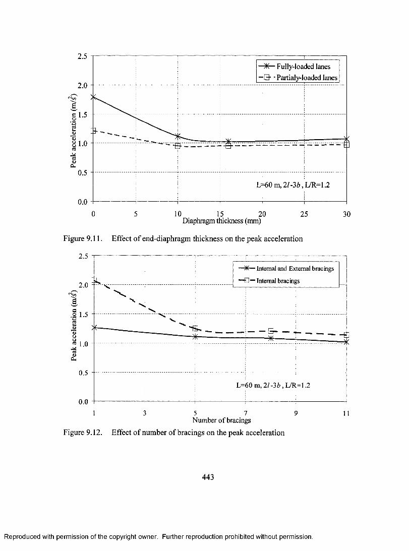
2.5X Fully-loaded lanes
—B- - Partialy-loaded lanes2.0
1.5
1.0
0.5L=60m,2/-36,iyR=1.2
0.00 10 155 20 25 30
Diaphragm thickness (mm)
Figure 9.11. Effect of end-diaphragm thickness on the peak acceleration
a_o
o
<uOh
2.5— — Internal and External bracings
Internal bracings2.0
1.5
Q— —-E ]
1.0
0.5
L=60 m ,2/-3i,L/R =1.2
0.0
1 3 5 7 9 I INumber of bracings
Figure 9.12. Effect of number of bracings on the peak acceleration
443
Reproduced with permission of the copyright owner. Further reproduction prohibited without permission.

Appendix A
A typical input data deck for the linear analysis of a bridge^ H E A D I N G2 B 0 X C U R V E D C O N T I N U O U S C A S E L = 2 0 , 2 L a n e ( A = 9 . 3 m ) , L / R = 0 . 4 * D A T A C H E C K* P R E P R I N T , E C H O = Y E S , M O D E L = N O , H I S T O R Y = N O ^ R E S T A R T , W R I T E* * * * * * * * * * * * R E F E R E N C E N O D E C O O R D I N A T E S F O R T H E L E F T S I D E * * * * * * * * * * * * * N O D E1 0 0 , 01 1 , 0 0 , - . 1 2 0 51 1 1 , 0 0 , - . 9 0 4 51 0 0 , 5 0 . 3 3 5 9 8 , 2 1 . 2 8 1 7 1 , 01 7 0 0 , 4 1 . 7 7 0 1 2 , 1 7 . 6 6 0 1 2 , 03 1 0 , 4 9 . 2 6 5 2 5 , 2 0 . 8 2 9 0 1 , - . 1 2 0 53 7 0 , 4 9 . 2 6 5 2 5 , 2 0 . 8 2 9 0 1 , - . 9 0 4 51 5 1 0 , 4 2 . 8 4 0 8 5 , 1 8 . 1 1 2 8 2 , - . 1 2 0 51 5 7 0 , 4 2 . 8 4 0 8 5 , 1 8 . 1 1 2 8 2 , - . 9 0 4 5********** R E F E R E N C E N O D E C O O R D I N A T E S F O R T H E R I G H T S I D E * * * * * * * * * * * * *7 2 0 1 0 0 ,7 2 1 7 0 0 ,7 2 0 3 1 0 ,7 2 0 3 7 0 ,7 2 1 5 1 0 ,7 2 1 5 7 0 ,
5 0 . 3 3 5 9 8 ,4 1 . 7 7 0 1 2 ,4 9 . 2 6 5 2 5 ,4 9 . 2 6 5 2 5 , 4 2 . 8 4 0 8 5 , 4 2 . 8 4 0 8 5 ,
- . 1 2 0 5 - . 9 0 4 5 - . 1 2 0 5 - . 9 0 4 5
- 2 1 . 2 8 1 7 1 ,- 1 7 . 6 6 0 1 2 ,- 2 0 . 8 2 9 0 1 ,- 2 0 . 8 2 9 0 1 ,- 1 8 . 1 1 2 8 2 ,- 1 8 . 1 1 2 8 2 ,
N O D E G E N* N G E N , N S E T = S L A B O U T , L I N E = C1 0 0 . 7 2 0 1 0 0 . 1 0 0 0 0 . 1 *NGEN,NSET=SLABIN,LINE=C1 7 0 0 . 7 2 1 7 0 0 . 1 0 0 0 0 . 1 * N F I L L , N S E T = S L A B S L A B O U T , S L A B I N , 1 6 , 1 0 0* * * * * * * * * * * * * * * * * * * * * * * N O D E G E N . F O R A L L T H E W E B S * N G E N , N S E T = W E B 0 U T 1 , L I N E = C3 1 0 . 7 2 0 3 1 0 . 1 0 0 0 0 . 1 1 * N G E N , N S E T = W E B 0 U T 2 , L I N E = C3 7 0 . 7 2 0 3 7 0 . 1 0 0 0 0 . 1 1 1 * N F I L L , N S E T = W E B O U T
W E B 0 U T 1 , W E B 0 U T 2 , 6 , 1 0 * N G E N , N S E T = W E B I N 1 , L I N E = C1 5 1 0 . 7 2 1 5 1 0 . 1 0 0 0 0 . 1 1 * N G E N , N S E T = W E B I N 2 , L I N E = C1 5 7 0 . 7 2 1 5 7 0 . 1 0 0 0 0 . 1 1 1 * N F I L L , N S E T = W E B I N
W E B I N l , W E B I N 2 , 6 , 1 0 * N F I L L , N S E T = W E B
W E B O U T , W E B I N , 3 , 4 0 0
* N F I L L , N S E T = A L L N O D E W E B O U T , W E B I N , 1 2 , 1 0 0 ************************ N F I L L , N S E T = F L A N T
W E B O U T l , W E B I N l , 3 , 4 0 0* * * * * * * * * * * * * * * * * * * * * * n o d e G E N . F O R T H E B O T T O M F L A N G E
F O R T H E S L A B * * * * * * * * * * * * * * * * * * * * *
•k'k'k'k-k-k'k'k'k-k-k'k'k'k-k'k'k'k'k-k
NODE GEN. FOR ALL NODES ■ 'fr'k-k-k-k'k'k'k-k-k'k'k-k-k'k'k'k'k-k
N O D E G E N . F O R T H E T O P F L A N G E
'k'k'k'k'k'k'k'k'k'k'k'k'k'k-k'k
444
Reproduced with permission of the copyright owner. Further reproduction prohibited without permission.

* N F I L L , N S E T = F L A N B W E B 0 U T 2 , W E B I N 2 , 1 2 , 1 0 0****'k-k-k-k-k-k*-k-kick'k'k-k-k-k-k-k-k-k-k-k-k-k-k'k'k'k'k-k'k-k-k'k'k'k-k-k-)ck'k-k-k*'k-Jr-^-)ck-^-k-k-k-k-k-k-*r'^-k-k*'k'k'k*-k'k
ELEMENT GEN. FOR TOP SLAB *******************^ E L E M E N T , T Y P E = S 4 R1 0 0 , 1 0 0 , 2 0 0 , 1 0 2 0 0 , 1 0 1 0 0* E L G E N , E L S E T = S L A B1 0 0 . 1 6 . 1 0 0 . 1 0 0 . 7 2 . 1 0 0 0 0 . 1 0 0 0 0* * * * * * * * * * * * * * * * * * * * * * * * * E L E M E N T G E N . F O R T O P F L A N G E * * * * * * * * * * * * * * * * * * * E L E M E N T , T Y P E = B 3 1 H3 1 0 . 1 0 3 1 0 . 3 1 0 * E L G E N , E L S E T = F L A N T3 1 0 , 4 , 4 0 0 , 4 0 0 , 7 2 , 1 0 0 0 0 , 1 0 0 0 0* * * * * * * * * * * * * * * * * * * * * * * * * * * * E L E M E N T G E N . F O R W E B S * * * * * * * * * * * * * * * * * * * *^ E L E M E N T , T Y P E = S 4 R3 2 0 , 3 1 0 , 3 2 0 , 1 0 3 2 0 , 1 0 3 1 0* E L G E N , E L S E T = W E B3 2 0 , 6 , 1 0 , 1 0 , 7 2 , 1 0 0 0 0 , 1 0 0 0 0 , 4 , 4 0 0 , 4 0 0* * * * * * * * * * * * * * * * * * * * * * * E L E M E N T G E N . F O R B O T T O M F L A N G E * * * * * * * * * * * * * * * ** E L E M E N T , T Y P E = S 4 R3 7 1 , 3 7 0 , 4 7 0 , 1 0 4 7 0 , 1 0 3 7 0* E L G E N , E L S E T = F L A N B 13 7 1 . 4 . 1 0 0 . 1 0 0 . 7 2 . 1 0 0 0 0 . 1 0 0 0 0* E L C O P Y , O L D S E T = F L A N B 1 , N E W S E T = F L A N B 2 , S H I F T N O D E S = 8 0 0 , E L E M E N T S H I F T = 8 0 0 * E L S E T , E L S E T = F L A N B F L A N B l , F L A N B 2* * * * * * * * * * * * * * * * * * * * * * * e l e m e n t G N . F O R E N D D I A P H R A G M * * * * * * * * * * * * * * * * ** E L E M E N T , T Y P E = S 4 R3 1 1 , 3 1 0 , 3 2 0 , 4 2 0 , 4 1 0* E L G E N , E L S E T = D I A P L 13 1 1 , 4 , 1 0 0 , 1 0 0 , 6 , 1 0 , 1 0* E L C O P Y , O L D S E T = D I A P L 1 , N E W S E T = D I A P L 2 , S H I F T N 0 D E S = 8 0 0 , E L E M E N T S H I F T = 8 0 0* E L S E T , E L S E T = D I A P L D I A P L l , D I A P L 2* E L C 0 P Y , 0 L D S E T = D I A P L , N E W S E T = D I A P M , S H I F T N O D E S = 3 6 0 0 0 0 , E L E M E N T S H I F T = 3 6 0 0 0 0* E L C O P Y , O L D S E T = D I A P M , N E W S E T = D I A P R , S H I F T N O D E S = 3 6 0 0 0 0 , E L E M E N TS H I F T = 3 6 0 0 0 0* E L S E T , E L S E T = D I A PD I A P L , D I A P M , D I A P R* * * * * * * * * * * * * * * * * * * * * * * * e n d f l a n g e E L E M E N T S * * * * * * * * * * * * * * * * * * * * * * * * * * * E L E M E N T , T Y P E = B 3 1 H3 1 2 . 4 1 0 . 3 1 0 * E L G E N , E L S E T = E F L A N L 13 1 2 , 4 , 1 0 0 , 1 0 0* E L C O P Y , O L D S E T = E F L A N L l , N E W S E T = E F L A N L 2 , S H I F T N 0 D E S = 8 0 0 , E L E M E N T S H I F T = 8 0 0* E L S E T , E L S E T = E F L A N L E F L A N L l , E F L A N L 2* E L C O P Y , O L D S E T = E F L A N L , N E W S E T = E F L A N R , S H I F T N O D E S = 7 2 0 0 0 0 , E L E M E N TS H I F T = 7 2 0 0 0 0*ELSET, ELSET=EFLAN
E F L A N L , E F L A N R* * * * * * * * * * * * * * * * * * * e l e m e n t g e n f o r t h e e n d t r u s s e l e m e n t s * * * * * * * * * * * *
^ELEMENT, T Y P E = B 3 1 H7 1 1 , 7 1 0 , 1 1 1 0* E L G E N , E L S E T = B R A C E7 1 1 , 2 , 6 0 , 6 0 , 3 , 3 6 0 0 0 0 , 3 6 0 0 0 0’ ^ E L E M E N T , T Y P E = B 3 1 H9 4 1 , 9 4 0 , 7 1 0*ELGEN, ELSET=BRACE9 4 1 , 2 , 2 3 0 , 1 , 3 , 3 6 0 0 0 0 , 3 6 0 0 0 0
445
Reproduced with permission of the copyright owner. Further reproduction prohibited without permission.

* E L E M E N T , T Y P E = B 3 1 H9 4 3 , 7 7 0 , 9 4 0*ELGEN,ELSET=BRACE9 4 3 , 2 , 1 7 0 , 1 , 3 , 3 6 0 0 0 0 , 3 6 0 0 0 0* * E L E M E N T G E N F O R T H E I N T E R . T R U S S E L E M E N T S * * * * * * * * * * * * * * E L E M E N T , T Y P E = B 3 1 H 9 0 3 1 1 , 9 0 3 1 0 , 9 0 7 1 0 * E L G E N , E L S E T = B R A C I9 0 3 1 1 . 3 . 4 0 0 . 4 0 0 . 3 , 9 0 0 0 0 , 9 0 0 0 0 ^ E L E M E N T , T Y P E = B 3 1 H , E L S E T = B R A C I 9 0 7 7 1 , 9 0 7 7 0 , 9 1 1 7 0*ELGEN,ELSET=BRACI9 0 7 7 1 . 3 , 9 0 0 0 0 , 9 0 0 0 0 ^ E L E M E N T , T Y P E = B 3 1 H 9 0 5 4 1 , 9 0 5 4 0 , 9 0 3 1 0 * E L G E N , E L S E T = B R A C I9 0 5 4 1 , 2 , 2 3 0 , 1 , 3 , 4 0 0 , 4 0 0 , 3 , 9 0 0 0 0 , 9 0 0 0 0 ^ E L E M E N T , T Y P E = B 3 1 H 9 0 5 4 3 , 9 0 3 7 0 , 9 0 5 4 0 * E L G E N , E L S E T = B R A C I9 0 5 4 3 . 2 . 1 7 0 . 1 . 3 . 4 0 0 . 4 0 0 . 3 , 9 0 0 0 0 , 9 0 0 0 0* E L C O P Y , O L D S E T = B R A C I , N E W S E T = B R A C I , S H I F T N 0 D E S = 3 6 0 0 0 0 , E L E M E N T S H I F T = 3 6 0 0 0 0* * * * * * * * * * * * * * * * * * * * * * * * * M A T E R I A L P R O P E R T I E S * * * * * * * * * * * * * * * * * * * * * * * * * ^ O R I E N T A T I O N , N A M E = L O C A L , S Y S T E M = C Y L I N D R I C A L 0 , 0 , - 1 0 , 0 , 0 , 1 0 3 , 0* S H E L L S E C T I O N , E L S E T = S L A B , M A T E R I A L = C O N , O R I E N T A T I O N = L O C A L
. 2 2 5 , 5^ M A T E R I A L , N A M E = C O N* D E N S I T Y2 . 4 0 0^ E L A S T I C2 7 E 6 , . 2 0* S H E L L S E C T I O N , E L S E T = F L A N B , M A T E R I A L = S T E E L , O R I E N T A T I O N = L O C A L . 0 1 6 , 5
* M A T E R I A L , N A M E = S T E E L* D E N S I T Y7 . 8 0 0^ E L A S T I C2 0 0 E 6 , . 3* S H E L L S E C T I O N , E L S E T = W E B , M A T E R I A L = S T E E L . 0 1 6 , 5
* B E A M S E C T I O N , S E C T I O N = R E C T , E L S E T = F L A N T , M A T E R I A L = S T E E L . 0 1 6 , . 3 0 , 0 , 15 . 5* B E A M S E C T I O N , S E C T I O N = R E C T , E L S E T = E F L A N , M A T E R I A L = S T E E L . 0 1 6 , . 3 0 , 0 , 15 . 5* S H E L L S E C T I O N , E L S E T = D I A P , M A T E R I A L = S T E E L . 0 1 6 , 5
* B E A M S E C T I O N , S E C T I O N = R E C T , E L S E T = B R A C E , M A T E R I A L = S T E E L . 1 , . 1 0 , 0 , 15 . 5*BEAM SECTION,SECTION=RECT,ELSET=BRACI,MATERIAL=STEEL . 1 , . 1 0 , 0 , 1 5 , 5•k-k-k'k'k'k'k'k'k-k'k-kit-k-k-k-k-k-k'k'k'k'k-k'k'k-k'k'k'k'k'k'k'k'k'k'k'k'k'k'k'k'k'k-k'k'k'k'k'k-k'k'k'k'k'k'k'k'k'k'k'k'k'k-k'k-k'k'k-k•k'k-k-k'k'k-k-k-*;-k-k-k-k'k-k-k-k-k-k-k-k'k'k'k'k'k- 'k |V[ULT J POINT CONSTRAINT
446
Reproduced with permission of the copyright owner. Further reproduction prohibited without permission.

* N G E N , N S E T = N S L A B O U T , L I N E = C3 0 0 . 7 2 0 3 0 0 . 1 0 0 0 0 . 1 * N G E N , N S E T = N S L A B I N , L I N E = C1 5 0 0 . 7 2 1 5 0 0 . 1 0 0 0 0 . 1 * N F I L L , N S E T = N S L A B
N S L A B O U T , N S L A B I N , 3 , 4 0 0 * N S E T , N S E T = N S L A B E L4 0 0 , 5 0 0 , 6 0 0 , 1 2 0 0 , 1 3 0 0 , 1 4 0 0 * N S E T , N S E T = N S L A B E R7 2 0 4 0 0 , 7 2 0 5 0 0 , 7 2 0 6 0 0 , 7 2 1 2 0 0 , 7 2 1 3 0 0 , 7 2 1 4 0 0 * N S E T , N S E T = N S L A B E M3 6 0 4 0 0 . 3 6 0 5 0 0 . 3 6 0 6 0 0 , 3 6 1 2 0 0 , 3 6 1 3 0 0 , 3 6 1 4 0 0 * N S E T , N S E T = N F L A N E L4 1 0 , 5 1 0 , 6 1 0 , 1 2 1 0 , 1 3 1 0 , 1 4 1 0 * N S E T , N S E T = N F L A N E R7 2 0 4 1 0 , 7 2 0 5 1 0 , 7 2 0 6 1 0 , 7 2 1 2 1 0 , 7 2 1 3 1 0 , 7 2 1 4 1 0 * N S E T , N S E T = N F L A N E M3 6 0 4 1 0 . 3 6 0 5 1 0 . 3 6 0 6 1 0 , 3 6 1 2 1 0 , 3 6 1 3 1 0 , 3 6 1 4 1 0 * M P CB E A M , N S L A B , F L A N T B E A M , N S L A B E L , N F L A N E L B E A M , N S L A B E M , N F L A N E M B E A M , N S L A B E R , N F L A N E R *******■********■*•■*■****************■*■***■*•*■*•*■*•■*•*•*****■*■**■*■*** + ******■*■* + *■*•*** N G E N , N S E T = S U P P 13 7 0 . 1 5 7 0 . 4 0 0 * N G E N , N S E T = S U P P 23 6 0 3 7 0 . 3 6 1 5 7 0 . 4 0 0 * N G E N , N S E T = S U P P 37 2 0 3 7 0 . 7 2 1 5 7 0 . 4 0 0 * N S E T , N S E T = S U P P S U P P l , S U P P 2 , S U P P 3 * T R A N S F O R M , N S E T = S U P P , T Y P E = C 4 6 . 5 1 2 5 , 0 , - 1 0 , 4 6 . 5 1 2 5 , 0 , 1 0 * B O U N D A R YS U P P , 3 S U P P 2 , 2 1 5 7 0 , 23 6 1 5 7 0 . 17 2 1 5 7 0 . 2* E L S E T , E L S E T = X B R A C B R A C E , B R A C I * N G E N , N S E T = M D1 4 0 3 7 0 . 1 4 1 5 7 0 . 1 0 0 * E L G E N , E L S E T = M S1 4 0 3 7 1 . 4 . 1 0 0 . 1 0 03 6 0 3 7 1 . 4 . 1 0 0 . 1 0 0 * E L G E N , E L S E T = M S1 4 1 1 7 1 . 4 . 1 0 0 . 1 0 03 6 1 1 7 1 . 4 . 1 0 0 . 1 0 0
a n a l y s i s ** S T E P
C A S E ( 2 ) : T Y P I C A L T R U C K L O A D I N G C A S E ^ S T A T I C*DLOAD, OP=NEW* N S E T , N S E T = C A S E 21 8 0 4 0 0 , 1 8 0 7 0 0* N S E T , N S E T = C A S E 22 0 4 0 0 , 1 0 0 4 0 0 , 2 0 7 0 0 , 1 0 0 7 0 0* C L O A D , O P = N E W
C A S E 2 , 3 , - 1 8C A S E 2 , 3 , - 7 1
447
Reproduced with permission of the copyright owner. Further reproduction prohibited without permission.

* N O D E P R I N T , N S E T = M D U 3* N O D E P R I N T , N S E T = S U P P R F 3* E L P R I N T , P O S I T I O N = A V E R A G E D A T N O D E S , E L S E T = M S 8 2 2* E L P R I N T , E L S E T = X B R A C S F l■k'k-k-k-k-k-k-k-k-k'k-k'k-^-^-k-k'k'k-^-k-k-h'k-k-k-k-k-k-k'k'k-k-k- 'k-k- 'k-k- ' 'k'k'k'k-k-k'k-k'k'k'k-k- 'k-k'k'k'fc'k'k'k'k'k'k-k'k'k'k* E N D S T E P• k ' k ' k ' k ' k - k ' k - k ' k ' k ' k - k ' k ' k ' k ' k ' k ' k - k ' k ' k ' k ' k ' k ' ^ j ^ Q Q v i k ) 2 r 3 . t i o r i* S T E P* F R E Q U E N C Y , E I G E N S O L V E R = S U B S P A C E 4■k'k-k-k-k'k-k'k'k-k'k-k'ick'k'k-k-k-k-k'k'k-k'k'k'k-^-k'k-k'k'k'k'k-k'k'k-k-k'k-k'k^'k-k'k'k-^'k-k'k'k-k-k'k'k-k'k'k'k' ie'k-k'^' if-k-k-k-k-k
^ O U T P U T , F I E L D* N O D E O U T P U T , N S E T = S L A BU' k ' k - k - k - k - k ' k ' k - k ' k ' k ' k ' k - k ' k ' k ' k - k i f i r ' k ' k ' k ' k ' k ' k - k ' k ' k ' k ' k - k i c ' k ' k i r ' k ' k ' k - k ' k - k ' k - k ' k - k - k ' k - k - k ' k ' k - k ' k ' k - k - k - k - k - k - k - k - k - k ' k - k - k ' k - k ' k
* E N D S T E P'k-k'k-k-k-:k'k'k-k-k'k'k'k-k-k-k'k-k-k-k-k-k'k-k'k-k'k-k-k- -k j_ Q SFlSlySiS* S T E P , I N C = 3 0 5 * D Y N A M I C . 0 2 , 6 . 1
* D L O A D S L O A D , P N U S L O A D , B X N U S L O A D , B Y N U-:)r-:k-k'k-k-k-k-k'k'k-kr)ir'k'k'k'k'k-k'k'k'k'k'k'k'k'k'k'k'k'k-k'k'k'k-k'k'k-k'k'k-k-k-k'k'k'k'k'^'k'k'k':)f'k-k-k-k^^'k-k^-k^'k'^-k-k-:k'k'k-k-:)<:
* O U T P U T , H I S T O R Y , F R E Q U E N C Y = 1 * E L E M E N T O U T P U T , E L S E T = A S T S 2 2^ E L E M E N T O U T P U T , E L S E T = S H E S F 3* N O D E O U T P U T , N S E T = D E F U 3* N O D E O U T P U T , N S E T = A R E
R F l , R F 2 , R F 3*************************************************************************** E N D S T E P
q u a s i - s t a t i c a n a l y s i s * * * * * * * * * * * * * * * * * * ** S T E P
C A S E ( 1 ) : M A X I M U M U L T I M A T E L O A D D U E T O N E G A T I V E M O M E N T ^ D Y N A M I C , E X P L I C I T , 1^ B O U N D A R Y , A M P L I T U D E = R A M P , T Y P E = D I S P L A C E M E N T C A S E l , 3 , 3 , - 1 .' k i f i f - k - k ' k ' k ' k i e ' k ' k ' k ' k - k - k - k ' k ' k - k - k - k - k ' k ' k ' k ' k ' k ' k ' k ' k ' k ' k - k ' k - k - k ' k - k ' k - k - k ' k ' k ' k ' k - k ' k ' k - k - k ' k ^ - k - k - k - k ' k ' k - k ' k - k ' k ' k - i e - k - k - ) f - k - k - k
^ O U T P U T , F I E L D , N U M B E R I N T E R V A L = 2 0 ^ E L E M E N T O U T P U T , P O S I T I O N = C E N T R O I D A L E , S^ E L E M E N T O U T P U T , R E B A R = L T O P E , S , R B F O R^ E L E M E N T O U T P U T , R E B A R = L B O T T O M E , S , R B F O R* E L E M E N T O U T P U T , R E B A R = T T O P E , S , R B F O R^ E L E M E N T O U T P U T , R E B A R = T B O T T O M
E , S , R B F O R * N O D E O U T P U T U
*ENDSTEP
448
Reproduced with permission of the copyright owner. Further reproduction prohibited without permission.

Appendix B
Samples of the results for the load distribution factors
Bridge ConfigurationDistribution Factor for
Positive StressL L /R N l Nb F.E.M. Eq. 7.120 0 2 2 1.03 1.1540 0 2 2 1.00 1.1560 0 2 2 1.01 1.1580 0 2 2 1.01 1.15too 0 2 2 1.02 1.1520 0 3 4 0.96 1.0640 0 3 4 0.93 1.0660 0 3 4 0.91 1.0680 0 3 4 0.91 1.06too 0 3 4 0.92 1.0620 0 3 5 0.98 1.0640 0 3 5 0.94 1.0660 0 3 5 0.92 1.0680 0 3 5 0.90 1.06too 0 3 5 0.92 1.0620 0 3 6 0.98 1.0640 0 3 6 0.93 1.0660 0 3 6 0.92 1.0680 0 3 6 0.91 1.06too 0 3 6 0.92 1.0620 0.4 2 2 1.10 1.1740 0.4 2 2 1.07 1.1860 0.4 2 2 1.01 1.1980 0.4 2 2 1.19 1.20too 0.4 2 2 1.14 1.2120 0.4 3 4 1.05 1.0840 0.4 3 4 0.98 1.1060 0.4 3 4 1.08 1.1180 0.4 3 4 1.14 1.12too 0.4 3 4 1.09 1.1320 0.4 4 6 1.02 1.0240 0.4 4 6 0.88 1.0460 0.4 4 6 0.93 1.0580 0.4 4 6 0.96 1.06too 0.4 4 6 0.95 1.0820 0.2 2 2 1.07 1.1540 0.2 2 2 1.02 1.1660 1.2 2 2 1.36 1.5180 1.2 2 2 1.66 1.59too 1.2 2 2 1.49 1.6720 0.2 3 4 1.00 1.0640 0.2 3 4 0.94 1.0760 1.2 3 4 1.52 1.5080 1.2 3 4 1.65 1.60too 1.2 3 4 1.54 1.70
449
Reproduced with permission of the copyright owner. Further reproduction prohibited without permission.
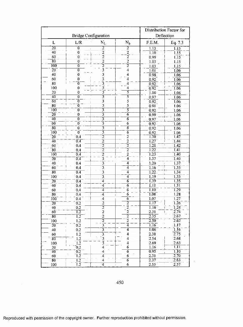
Bridge ConfigurationDistribution Factor for
DeflectionL L/R Nl Nb F.E.M. Eq. 7.320 0 2 2 1.13 1.1540 0 2 2 1.10 1.1560 0 2 2 0.99 1.1580 0 2 2 1.03 1.15100 0 2 2 1.03 1.1520 0 3 4 1.01 1.0640 0 3 4 0.98 1.0660 0 3 4 0.92 1.0680 0 3 4 0.92 1.06100 0 3 4 0.92 1.0620 0 3 5 1.00 1.0640 0 3 5 0.97 1.0660 0 3 5 0.92 1.0680 0 3 5 0.91 1.06100 0 3 5 0.92 1.0620 0 3 6 0.99 1.0640 0 3 6 0.97 1.0660 0 3 6 0.92 1.0680 0 3 6 0.92 1.06100 0 3 6 0.92 1.0620 0.4 2 2 1.30 ^ 1.4740 0.4 2 2 1.27 1.4460 0.4 2 2 1.21 1.4280 0.4 2 2 1.22 1.41100 0.4 2 2 1.23 1.4020 0.4 3 4 1.37 1.4040 0.4 3 4 1.20 1.3760 0.4 3 4 1.16 1.3580 0.4 3 4 1.22 1.34100 0.4 3 4 1.19 1.3320 0.4 4 6 1.39 1.3540 0.4 4 6 1.11 1.3160 0.4 4 6 1.10 1.2980 0.4 4 6 1.08 1.28too 0.4 4 6 1.07 1.2720 0.2 2 2 1.17 1.2640 0.2 2 2 1.16 1.2460 1.2 2 2 2.31 2.7480 1.2 2 2 2.35 2.67100 1.2 2 2 2.50 2.6220 0.2 3 4 1.16 1.1740 0.2 3 4 1.06 1.1660 1.2 3 4 2.38 2.7580 1.2 3 4 2.54 2.68100 1.2 3 ^ 4 2.69 2.63
'2 0 0.2 4 6 1.16 f.ll40 0.2 4 6 0.95 1.1060 1.2 4 6 2.31 2.7080 1.2 4 6 2.37 2.63100 1.2 4 6 2.55 2.57
450
Reproduced with permission of the copyright owner. Further reproduction prohibited without permission.
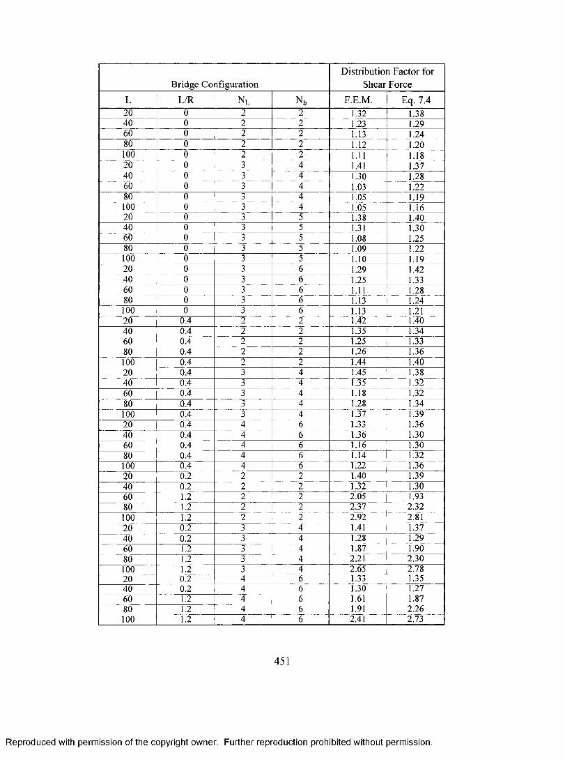
Bridge ConfigurationDistribution Factor for
Shear ForceL L /R N l Nb F.E.M. Eq. 7.420 0 2 2 1.32 1.3840 0 2 2 1.23 1.2960 0 2 2 1.13 1.2480 0 2 2 1.12 1.20100 0 2 2 1.11 1.1820 0 3 4 1.41 1.3740 0 3 4 1.30 1.2860 0 3 4 1.03 1.2280 0 3 4 1.05 1.19too 0 3 4 1.05 1.1620 0 3 5 1.38 1.4040 0 3 5 1.31 1.3060 0 3 5 1.08 1.2580 0 3 5 1.09 1.22too 0 3 5 1.10 1.1920 0 3 6 1.29 1.4240 0 3 6 1.25 1.3360 0 3 6 1.11 1.2880 0 3 6 1.13 1.24too 0 3 6 1.13 1.2120 0.4 2 2 1.42 1.4040 0.4 2 2 1.35 1.3460 0.4 2 2 1.25 1.3380 0.4 2 2 1.26 1.36too 0.4 2 2 1.44 M O20 0.4 3 4 1.45 1.3840 0.4 3 4 1.35 1.3260 0.4 3 ^ 4 1.18 1.3280 0.4 3 4 1.28 1.34too 0.4 3 4 1.37 1.3920 0.4 4 6 1.33 1.3640 0.4 4 6 1.36 1.3060 0.4 4 6 1.16 1.3080 0.4 4 6 1.14 1.32too 0.4 4 6 1.22 1.3620 0.2 2 2 1.40 1.3940 0.2 2 2 1.32 1.3060 1.2 2 2 2.05 1.9380 1.2 2 2 2.37 2.32100 1.2 2 2 2.92 2.8120 0.2 3 4 1.41 1.3740 0.2 3 4 1.28 1.2960 1.2 3 4 1.87 1.9080 1.2 3 4 2.21 2.30100 1.2 3 4 2.65 2.7820 0 2 4 6 1.33 1.3540 0.2 4 6 1.30 1.2760 1.2 4 6 1.61 1.8780 1.2 4 6 1.91 2.26100 1.2 4 6 2.41 2.73
451
Reproduced with permission of the copyright owner. Further reproduction prohibited without permission.
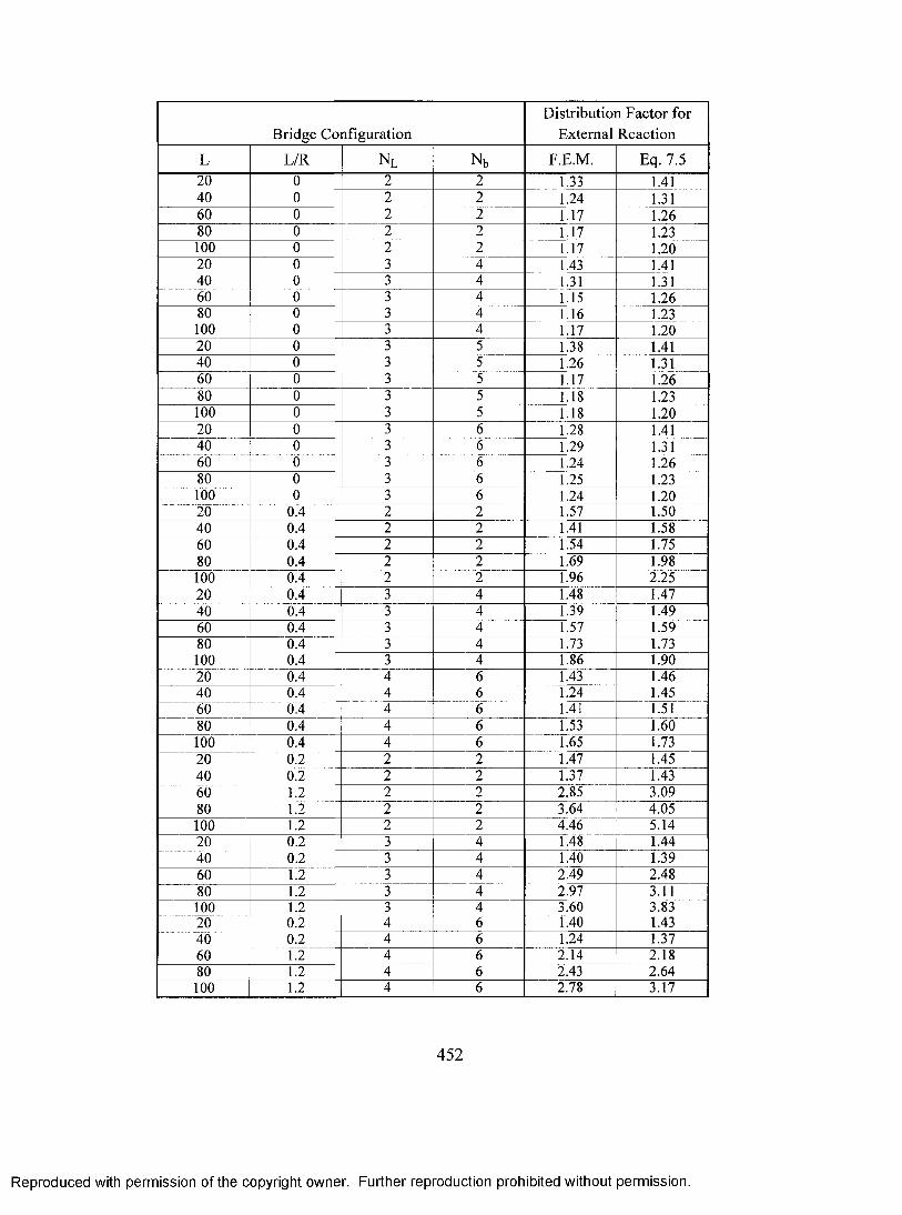
Bridge ConfigurationDistribution Factor for
External Reaction
L L/R Nl Nb F.E.M. Eq. 7.520 0 2 2 1.33 1.4140 0 2 2 1.24 1.3160 0 2 2 1.17 1.2680 0 2 2 1.17 1.23too 0 2 2 1.17 1.2020 0 3 4 1.43 1.4140 0 3 4 1.31 1.3160 0 3 4 1.15 1.2680 0 3 4 1.16 1.23too 0 3 4 1.17 1.2020 0 3 5 1.38 1.4140 0 3 5 1.26 1.3160 0 3 5 1.17 1.2680 0 3 5 1.18 1.23too 0 3 5 1.18 1.2020 0 3 6 1.28 1.4140 0 3 6 1.29 1.3160 0 3 6 1.24 1.2680 0 3 6 1.25 1.23too 0 3 6 1.24 1.2020 0.4 2 2 1.57 1.5040 0.4 2 2 1.41 1.5860 0.4 2 2 1.54 1.7580 0.4 2 2 1.69 1.98too 0.4 2 2 1.96 2.2520 0.4 3 4 1.48 1.4740 0.4 3 4 1.39 1.4960 0.4 3 4 1.57 1.5980 0.4 3 4 1.73 1.73100 0.4 3 4 1.86 1.9020 0.4 4 6 1.43 1.4640 0.4 4 6 1.24 1.4560 0.4 4 6 1.41 1.5180 0.4 4 6 1.53 1.60too 0.4 4 6 1.65 1.7320 0.2 2 2 1.47 1.4540 0.2 r 2 2 1.37 1.4360 1.2 2 2 2.85 3.0980 1.2 2 2 3.64 4.05too 1.2 2 2 4.46 5.1420 0.2 3 4 1.48 1.4440 0.2 3 4 1.40 1.3960 1.2 3 4 2,49 2.4880 1.2 3 4 2.97 3.11100 1.2 3 4 3.60 3.8320 0.2 4 6 1.40 1.4340 0.2 4 6 1.24 1.3760 1.2 4 6 2.14 2.1880 1.2 4 6 2.43 2.64100 1.2 4 6 2.78 3.17
452
Reproduced with permission of the copyright owner. Further reproduction prohibited without permission.
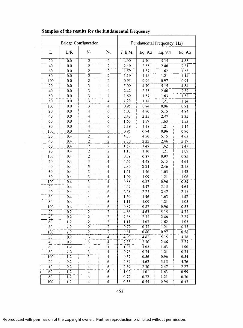
Samples of the results for the fundamental frequency
Bridge Configuration Fundamental Frequency (Hz)
L L/R Nl Nb F.E.M. Eq. 9.2 Eq. 9.4 Eq. 9.5
20 0.0 2 2 4.90 4.70 5.15 4.8540 0.0 2 2 2.40 2.35 2.46 2.3160 0.0 2 2 ^ 1.59 1.57 1.62 1.5380 0.0 2 2 1.19 1.18 1.21 1.14too 0.0 2 2 0.95 0.94 0.97 0.9120 0.0 3 4 5.00 4.70 5.15 4.8440 0.0 3 4 2.42 2.35 2.46 2.3260 0.0 3 4 1.60 1.57 1.63 1.5380 0.0 3 4 1.20 1.18 1.21 1.14too 0.0 3 4 0.95 0.94 0.96 0.9120 0.0 4 6 5.03 4.70 5.15 4.8440 0.0 4 6 2.43 2.35 2.47 2.3260 0.0 4 6 1.60 1.57 1.63 1.5380 0.0 4 6 1.19 1.18 1.21 1.14too 0.0 4 6 0.95 0.94 0.96 0.9020 0.4 2 2 4.70 4.50 5.15 4.6340 0.4 2 2 2.30 2.22 2.46 2.1960 0.4 2 2 1.52 1.47 1.62 1.4380 0.4 2 2 1.13 1.10 1.21 1.07too 0.4 2 2 0.89 0.87 0.97 0.8520 0.4 3 4 4.65 4.48 5.15 4.6140 0.4 3 4 2.30 2.21 2.46 2.1860 0.4 3 4 1.51 1.46 1.63 1.4380 0.4 3 4 1.09 1.09 1.21 1.06too 0.4 3 4 0.88 0.87 0.96 0.8420 0.4 4 6 4.49 4.47 5.15 4.6140 0.4 4 6 2.28 2.21 2.47 2.1860 0.4 4 6 1.50 1.46 1.63 1.4280 0.4 4 6 1.11 1.09 1.21 1.05too 0.4 4 6 0.87 0.87 0.96 0.8320 0.2 2 2 4.86 4.63 5.15 4.7740 0.2 2 2 2.38 2.31 ^ 2.46 2.2760 1.2 2 2 1.11 1.07 1.62 1.0580 1.2 2 2 0.79 0.77 1.21 0.75too 1.2 2 2 0.61 0.60 0.97 0.5820 0.2 3 4 4.90 4.62 5.15 4.7640 0.2 3 4 2.38 2.30 2.46 2.2760 1.2 3 4 1.05 1.03 1.63 1.0080 1.2 3 4 0.75 0.74 1.21 0.71too 1.2 3 4 0.57 0.56 0.96 ^ 0.5420 0.2 4 6 4.87 4.62 5.15 4.7640 0.2 4 6 2.39 2.30 2.47 2.2760 1.2 4 6 1.02 1.01 1.63 0.9980 1.2 4 6 0.72 0.72 1.21 0.70too 1.2 4 6 0.55 0.55 0.96 0.53
453
Reproduced with permission of the copyright owner. Further reproduction prohibited without permission.

Vita Auctoris
Magdy Said Samaan
1967 Born on the 31 of December in Cairo, Egypt.
1989 Graduated with B.Sc. degree (very good with Honours) in Civil Engineering
from Alexandria University, Alexandria, Egypt.
1990-1996 Worked as a Structural Engineer in several Consulting Engineering
Companies, Egypt.
1998 Graduated with M.Sc. degree in Civil Engineering, Hannover University,
Hannover, Germany.
1999 Worked as a Structural Engineer in an Infrastructure Engineering Company,
Germany.
2000 Enrolled as a full-time graduate student at the University of Windsor in the
Department of Civil and Environmental Engineering pursuing a Ph.D.
degree in Civil Engineering.
454
Reproduced with permission of the copyright owner. Further reproduction prohibited without permission.
Related Documents