Dynamic Agricultural Supply Response Under Economic Transformation: A Case Study of Henan, China

IFPRI Discussion Paper 00987

May 2010

Dynamic Agricultural Supply Response Under Economic Transformation

A Case Study of Henan Province

Bingxin Yu

Fengwei Liu

Liangzhi You

Development Strategy and Governance Division

INTERNATIONAL FOOD POLICY RESEARCH INSTITUTE

The International Food Policy Research Institute (IFPRI) was established in 1975. IFPRI is one of 15

agricultural research centers that receive principal funding from governments, private foundations, and

international and regional organizations, most of which are members of the Consultative Group on

International Agricultural Research (CGIAR).

PARTNERS AND CONTRIBUTORS

IFPRI gratefully acknowledges the generous unrestricted funding from Australia, Canada, China,

Denmark, Finland, France, Germany, India, Ireland, Italy, Japan, the Netherlands, Norway, the

Philippines, South Africa, Sweden, Switzerland, the United Kingdom, the United States, and the World

Bank.

AUTHORS

Bingxin Yu, International Food Policy Research Institute

Postdoctoral Fellow, Development Strategy and Governance Division

[email protected]

Fengwei Liu, Zhengzhou University of Light Industry

Associate Professor, School of Economics and Management

Liangzhi You, International Food Policy Research Institute

Senior Scientist, Enviornment Production and Technology Division

[email protected]

Notices 1 Effective January 2007, the Discussion Paper series within each division and the Director General’s Office of IFPRI

were merged into one IFPRI–wide Discussion Paper series. The new series begins with number 00689, reflecting the prior publication of 688 discussion papers within the dispersed series. The earlier series are available on IFPRI’s website at www.ifpri.org/pubs/otherpubs.htm#dp. 2 IFPRI Discussion Papers contain preliminary material and research results. They have been peer reviewed, but

have not been subject to a formal external review via IFPRI’s Publications Review Committee. They are circulated in order to stimulate discussion and critical comment; any opinions expressed are those of the author(s) and do not necessarily reflect the policies or opinions of IFPRI.

Copyright 2010 International Food Policy Research Institute. All rights reserved. Sections of this material may be reproduced for personal and not-for-profit use without the express written permission of but with acknowledgment to IFPRI. To reproduce the material contained herein for profit or commercial use requires express written permission. To obtain permission, contact the Communications Division at [email protected].

mailto:[email protected]


iii

Contents

Abstract v

1. Introduction 1

2. Background 2

3. Theoretical and Analytical Developments 1

4. Data and Variables 6

5. Empirical Analysis of Acreage, Yield, and Supply Response 9

6. Conclusion 18

References 20

iv

List of Tables

1. Agricultural production in Henan province, 1978–2007 3

2. Real output prices and input costs in Henan province, 1998–2007 6

3. Elasticity estimates in supply function from previous studies 8

4. Sample representation 6

5. Variable definitions 7

6. Growth of subsector crops in Henan province, 1998–2007 8

7. Panel unit test 9

8a. Area and yield response in Henan province, 1998–2007 10

8b. Area and yield response in Henan province with telephone access, 2001–2006 11

9. Short- and long-run elasticities in Henan province, 1998–2007 14

10a. Short- and long-run grain elasticities by zone, 1998–2007 15

10b. Short- and long-run cotton elasticities by zone, 1998–2007 16

10c. Short- and long-run oilcrops elasticities by zone, 1998–2007 17

List of Figures

1. Agroecological zones of Henan province 2

2a. Cropping patterns in Henan province, 1998–2007 4

2b. Cropping patterns in Henan province by zone, 1998 versus 2007 4

3. Growth in grain output, area, and yield in Henan province, 1978–2007 5

4. Grain yield in tons per hectare in Henan province, 1998–2007 5

v

ABSTRACT

China has experienced dramatic economic transformation and is facing the challenge of ensuring steady

agricultural growth. This study examines the crop sector by estimating the supply response for major

crops in Henan province from 1998 to 2007. We use a Nerlovian adjustment adaptive expectation model.

The estimation uses dynamic Generalized Method of Moments (GMM) panel estimation based on pooled

data across 108 counties. We estimate acreage and yield response functions and derive the supply

response elasticities. This research links supply response to exogenous factors (weather, irrigation,

government policy, capital investment, and infrastructure) and endogenous factors (prices). The

significant feature of the model specification used in the study is that it addresses the endogeneity

problem by capturing different responses to own- and cross-prices. Empirical results illustrate that there is

still great potential to increase crop production through improvement of investment priorities and proper

government policy. We confirm that farmers respond to price by both reallocating land and more

intensively applying non-land inputs to boost yield. Investment in rural infrastructure, human capacity,

and technology are highlighted as major drivers for yield increase. Policy incentives such as taxes and

subsidies prove to be effective in encouraging grain production.

Key words: dynamic panel model, supply elasticity, acreage and yield response, Generalized

Method of Moments (GMM)

JEL Code: D24, C23, Q11

1

1. INTRODUCTION

The Chinese economy has experienced dramatic transformation in the last few decades. Rapid

urbanization and dietary change, coupled with continuous population growth, have resulted in expanding

food demand. At the same time, declining agricultural land availability makes grain self-sufficiency, one

of the major goals of Chinese agriculture, a considerable challenge. In order to increase output, the

government implements comprehensive policies to encourage domestic agricultural supply. For example,

the agricultural tax was eliminated countrywide in 2005, reducing production costs for farmers. China has

established minimum government procurement prices for such major grain crops as rice and wheat. The

minimum procurement price of wheat increased by about 4 percent in 2008 and by 15 percent in 2009 to

reflect higher market price and increased production cost. The central government also provides direct

subsidies to rice, wheat, and maize farmers based on land area dedicated to grain cultivation. In addition,

the central government provides direct fiscal subsidies to major grain-producing counties to ensure high

and steady grain production. Since the implementation of the stimulus package in early 2009, the Chinese

central government has allocated 21 percent of additional investment, or US$18.7 billion, to rural

infrastructure and public services (Ministry of Finance of China 2009).

Despite this record, it remains unclear whether these policies are effective in stimulating grain

supply. There is a need for more knowledge of the structural parameters to guide economic policy

formulation, especially in light of the urgent need to increase production and farmers’ income under

economic transformation. Information on the agricultural sector’s supply response to changes in prices

and rural infrastructure may help policymakers to advance the process of poverty reduction and

modernization. If agriculture is highly responsive to policies, policy-induced changes in farmers’ response

could be effective in increasing production, which in turn could assist in ensuring long-term food security

in the country. This study aims to understand the effect of economic transformation on the supply

responsiveness of the agricultural sector under the new agricultural policies in China, using Henan

province as a case study.

This paper provides some empirical analysis of major crop production in China through

estimation of supplies responses to changes in price and non-price factors. It contributes to the literature

of supply response analysis in several ways. First, it updates the literature of agricultural production by

using the latest data and policy variables from one major grain-producing province in China, allowing us

to assess the grain sector under the drastic transformation that occurred over the last decade. Second, it

evaluates whether China has exhausted its production potential in the grain sector. It addresses this issue

by examining the extent to which grain producers respond to price changes after the implementation of

new agricultural policies and by comparing the flexibility of supply response under different policy

regimes. It thus identifies constraints in crop production in response to potential policy interventions.

Third, this study directly addresses the endogeneity problem in supply response analysis, which has been

mostly neglected in the past due to limits in either methodology development or computation power.

Panel data are used for this empirical study because they have the distinct advantage of providing spatial

and temporal variations. A dynamic panel data approach is chosen to tackle the endogeneity problem with

a consistent Generalized Method of Moments (GMM) estimator. Finally, the resulting models expand the

supply elasticity estimates for comparison across studies, making it easier to assess the validity of earlier

results.

The paper is organized as follows: Following this introduction are reviews of the agricultural

sector in Henan province and of past studies. Section three describes the theoretical framework and the

dynamic panel GMM method. Section four presents data and definitions of variables, and section five

reports empirical results. The final section summarizes conclusions and makes recommendations for

policy and future research.

2

2. BACKGROUND

Agriculture in Henan Province

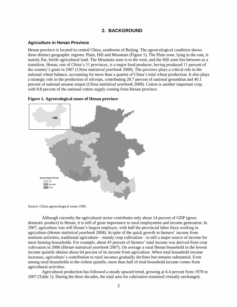
Henan province is located in central China, southwest of Beijing. The agroecological condition shows

three distinct geographic regions: Plain, Hill and Mountain (Figure 1). The Plain zone, lying in the east, is

mainly flat, fertile agricultural land. The Mountain zone is to the west, and the Hill zone lies between as a

transition. Henan, one of China’s 31 provinces, is a major food producer, having produced 11 percent of

the country’s grain in 2007 (China statistical yearbook 2008). The province plays a critical role in the

national wheat balance, accounting for more than a quarter of China’s total wheat production. It also plays

a strategic role in the production of oilcrops, contributing 28.7 percent of national groundnut and 40.1

percent of national sesame output (China statistical yearbook 2008). Cotton is another important crop,

with 9.8 percent of the national cotton supply coming from Henan province.

Figure 1. Agroecological zones of Henan province

Source: China agroecological zones 1985.

Although currently the agricultural sector contributes only about 14 percent of GDP (gross

domestic product) in Henan, it is still of great importance to rural employment and income generation. In

2007, agriculture was still Henan’s largest employer, with half the provincial labor force working in

agriculture (Henan statistical yearbook 2008). In spite of the quick growth in farmers’ income from

nonfarm activities, traditional agriculture—mainly crop cultivation—is still a major source of income for

most farming households. For example, about 45 percent of farmers’ total income was derived from crop

cultivation in 2006 (Henan statistical yearbook 2007). On average a rural Henan household in the lowest

income quintile obtains about 64 percent of its income from agriculture. When total household income

increases, agriculture’s contribution to rural incomes gradually declines but remains substantial. Even

among rural households in the richest quintile, more than half of total household income comes from

agricultural activities.

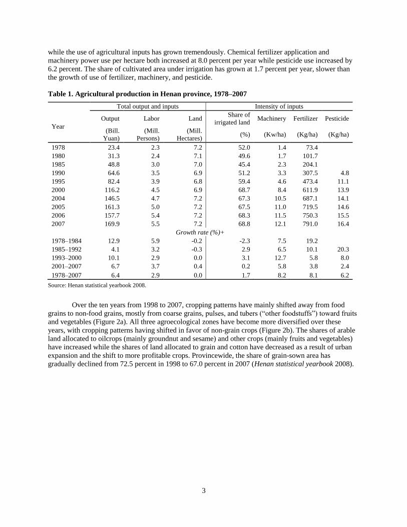
Agricultural production has followed a steady upward trend, growing at 6.4 percent from 1978 to

2007 (Table 1). During the three decades, the total area for cultivation remained virtually unchanged,

3

while the use of agricultural inputs has grown tremendously. Chemical fertilizer application and

machinery power use per hectare both increased at 8.0 percent per year while pesticide use increased by

6.2 percent. The share of cultivated area under irrigation has grown at 1.7 percent per year, slower than

the growth of use of fertilizer, machinery, and pesticide.

Table 1. Agricultural production in Henan province, 1978–2007

Total output and inputs Intensity of inputs

Year

Output Labor Land Share of

irrigated land Machinery Fertilizer Pesticide

(Bill.

Yuan)

(Mill.

Persons)

(Mill.

Hectares) (%) (Kw/ha) (Kg/ha) (Kg/ha)

1978 23.4 2.3 7.2 52.0 1.4 73.4

1980 31.3 2.4 7.1 49.6 1.7 101.7

1985 48.8 3.0 7.0 45.4 2.3 204.1

1990 64.6 3.5 6.9 51.2 3.3 307.5 4.8

1995 82.4 3.9 6.8 59.4 4.6 473.4 11.1

2000 116.2 4.5 6.9 68.7 8.4 611.9 13.9

2004 146.5 4.7 7.2 67.3 10.5 687.1 14.1

2005 161.3 5.0 7.2 67.5 11.0 719.5 14.6

2006 157.7 5.4 7.2 68.3 11.5 750.3 15.5

2007 169.9 5.5 7.2 68.8 12.1 791.0 16.4

Growth rate (%)+

1978–1984 12.9 5.9 -0.2 -2.3 7.5 19.2

1985–1992 4.1 3.2 -0.3 2.9 6.5 10.1 20.3

1993–2000 10.1 2.9 0.0 3.1 12.7 5.8 8.0

2001–2007 6.7 3.7 0.4 0.2 5.8 3.8 2.4

1978–2007 6.4 2.9 0.0 1.7 8.2 8.1 6.2

Source: Henan statistical yearbook 2008.

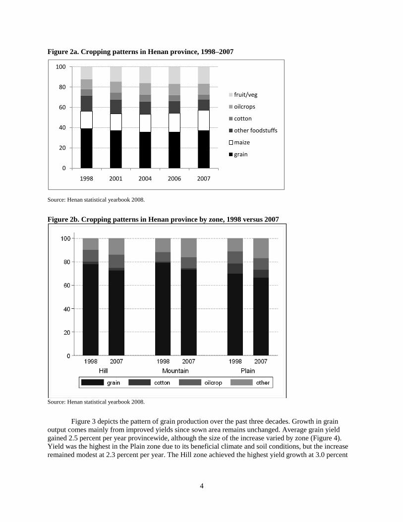
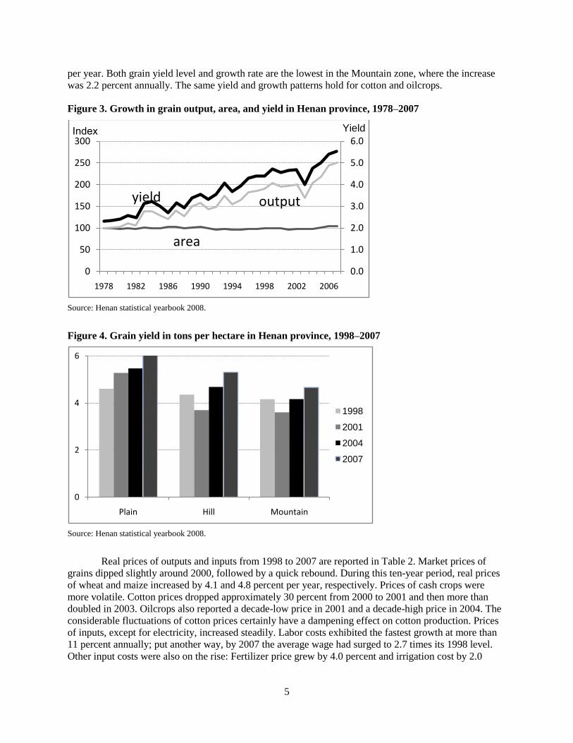
Over the ten years from 1998 to 2007, cropping patterns have mainly shifted away from food

grains to non-food grains, mostly from coarse grains, pulses, and tubers (―other foodstuffs‖) toward fruits

and vegetables (Figure 2a). All three agroecological zones have become more diversified over these

years, with cropping patterns having shifted in favor of non-grain crops (Figure 2b). The shares of arable

land allocated to oilcrops (mainly groundnut and sesame) and other crops (mainly fruits and vegetables)

have increased while the shares of land allocated to grain and cotton have decreased as a result of urban

expansion and the shift to more profitable crops. Provincewide, the share of grain-sown area has

gradually declined from 72.5 percent in 1998 to 67.0 percent in 2007 (Henan statistical yearbook 2008).

4

Figure 2a. Cropping patterns in Henan province, 1998–2007


Figure 2b. Cropping patterns in Henan province by zone, 1998 versus 2007


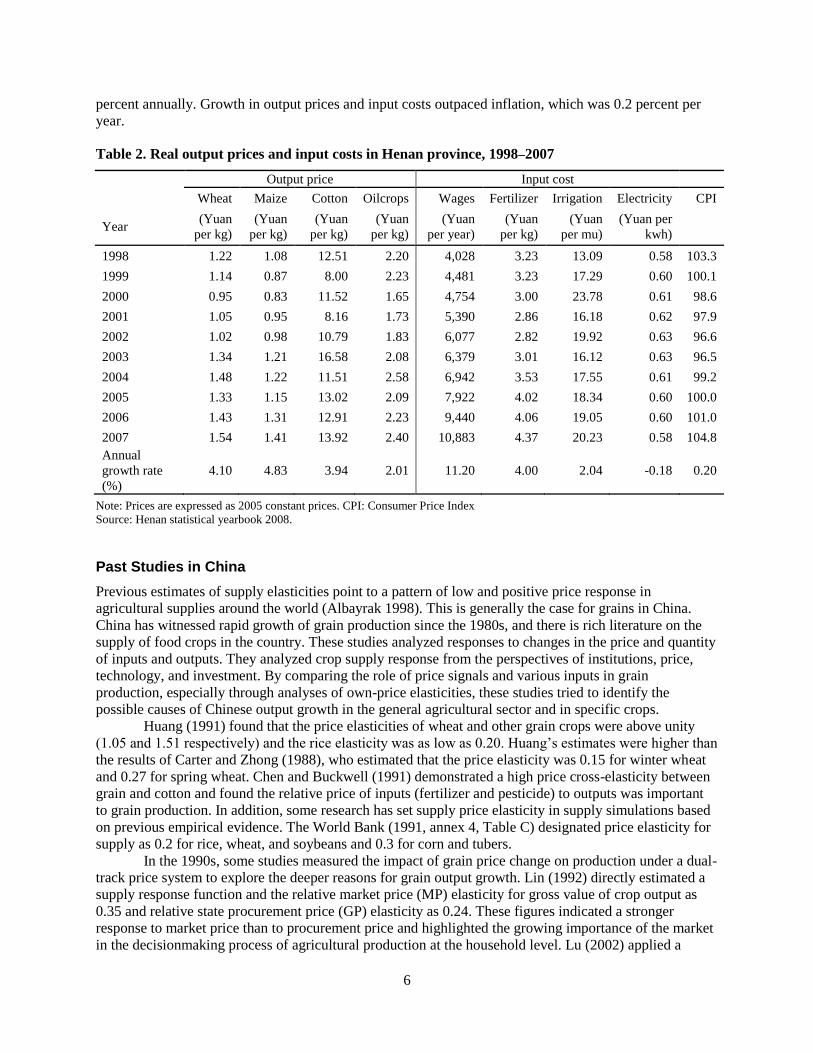
Figure 3 depicts the pattern of grain production over the past three decades. Growth in grain

output comes mainly from improved yields since sown area remains unchanged. Average grain yield

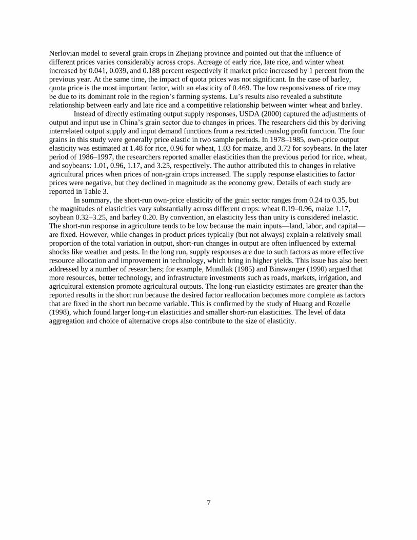
gained 2.5 percent per year provincewide, although the size of the increase varied by zone (Figure 4).

Yield was the highest in the Plain zone due to its beneficial climate and soil conditions, but the increase

remained modest at 2.3 percent per year. The Hill zone achieved the highest yield growth at 3.0 percent

0

20

40

60

80

100

1998 2001 2004 2006 2007

fruit/veg

oilcrops

cotton

other foodstuffs

maize

grain

5

per year. Both grain yield level and growth rate are the lowest in the Mountain zone, where the increase

was 2.2 percent annually. The same yield and growth patterns hold for cotton and oilcrops.

Figure 3. Growth in grain output, area, and yield in Henan province, 1978–2007


Figure 4. Grain yield in tons per hectare in Henan province, 1998–2007


Real prices of outputs and inputs from 1998 to 2007 are reported in Table 2. Market prices of

grains dipped slightly around 2000, followed by a quick rebound. During this ten-year period, real prices

of wheat and maize increased by 4.1 and 4.8 percent per year, respectively. Prices of cash crops were

more volatile. Cotton prices dropped approximately 30 percent from 2000 to 2001 and then more than

doubled in 2003. Oilcrops also reported a decade-low price in 2001 and a decade-high price in 2004. The

considerable fluctuations of cotton prices certainly have a dampening effect on cotton production. Prices

of inputs, except for electricity, increased steadily. Labor costs exhibited the fastest growth at more than

11 percent annually; put another way, by 2007 the average wage had surged to 2.7 times its 1998 level.

Other input costs were also on the rise: Fertilizer price grew by 4.0 percent and irrigation cost by 2.0

0.0

1.0

2.0

3.0

4.0

5.0

6.0

0

50

100

150

200

250

300

1978 1982 1986 1990 1994 1998 2002 2006

Yield Index

yield output

area

0

2

4

6

Plain Hill Mountain

1998

2001

2004

2007

6

percent annually. Growth in output prices and input costs outpaced inflation, which was 0.2 percent per

year.

Table 2. Real output prices and input costs in Henan province, 1998–2007

Output price Input cost

Wheat Maize Cotton Oilcrops Wages Fertilizer Irrigation Electricity CPI

Year (Yuan

per kg)

(Yuan

per kg)

(Yuan

per kg)

(Yuan

per kg)

(Yuan

per year)

(Yuan

per kg)

(Yuan

per mu)

(Yuan per

kwh)

1998 1.22 1.08 12.51 2.20 4,028 3.23 13.09 0.58 103.3

1999 1.14 0.87 8.00 2.23 4,481 3.23 17.29 0.60 100.1

2000 0.95 0.83 11.52 1.65 4,754 3.00 23.78 0.61 98.6

2001 1.05 0.95 8.16 1.73 5,390 2.86 16.18 0.62 97.9

2002 1.02 0.98 10.79 1.83 6,077 2.82 19.92 0.63 96.6

2003 1.34 1.21 16.58 2.08 6,379 3.01 16.12 0.63 96.5

2004 1.48 1.22 11.51 2.58 6,942 3.53 17.55 0.61 99.2

2005 1.33 1.15 13.02 2.09 7,922 4.02 18.34 0.60 100.0

2006 1.43 1.31 12.91 2.23 9,440 4.06 19.05 0.60 101.0

2007 1.54 1.41 13.92 2.40 10,883 4.37 20.23 0.58 104.8

Annual

growth rate

(%)

4.10 4.83 3.94 2.01 11.20 4.00 2.04 -0.18 0.20

Note: Prices are expressed as 2005 constant prices. CPI: Consumer Price Index


Past Studies in China

Previous estimates of supply elasticities point to a pattern of low and positive price response in

agricultural supplies around the world (Albayrak 1998). This is generally the case for grains in China.

China has witnessed rapid growth of grain production since the 1980s, and there is rich literature on the

supply of food crops in the country. These studies analyzed responses to changes in the price and quantity

of inputs and outputs. They analyzed crop supply response from the perspectives of institutions, price,

technology, and investment. By comparing the role of price signals and various inputs in grain

production, especially through analyses of own-price elasticities, these studies tried to identify the

possible causes of Chinese output growth in the general agricultural sector and in specific crops.

Huang (1991) found that the price elasticities of wheat and other grain crops were above unity

(1.05 and 1.51 respectively) and the rice elasticity was as low as 0.20. Huang’s estimates were higher than

the results of Carter and Zhong (1988), who estimated that the price elasticity was 0.15 for winter wheat

and 0.27 for spring wheat. Chen and Buckwell (1991) demonstrated a high price cross-elasticity between

grain and cotton and found the relative price of inputs (fertilizer and pesticide) to outputs was important

to grain production. In addition, some research has set supply price elasticity in supply simulations based

on previous empirical evidence. The World Bank (1991, annex 4, Table C) designated price elasticity for

supply as 0.2 for rice, wheat, and soybeans and 0.3 for corn and tubers.

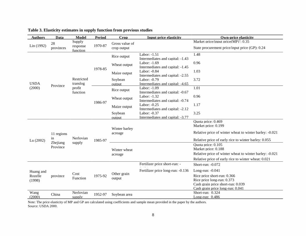
In the 1990s, some studies measured the impact of grain price change on production under a dual-

track price system to explore the deeper reasons for grain output growth. Lin (1992) directly estimated a

supply response function and the relative market price (MP) elasticity for gross value of crop output as

0.35 and relative state procurement price (GP) elasticity as 0.24. These figures indicated a stronger

response to market price than to procurement price and highlighted the growing importance of the market

in the decisionmaking process of agricultural production at the household level. Lu (2002) applied a

7

Nerlovian model to several grain crops in Zhejiang province and pointed out that the influence of

different prices varies considerably across crops. Acreage of early rice, late rice, and winter wheat

increased by 0.041, 0.039, and 0.188 percent respectively if market price increased by 1 percent from the

previous year. At the same time, the impact of quota prices was not significant. In the case of barley,

quota price is the most important factor, with an elasticity of 0.469. The low responsiveness of rice may

be due to its dominant role in the region’s farming systems. Lu’s results also revealed a substitute

relationship between early and late rice and a competitive relationship between winter wheat and barley.

Instead of directly estimating output supply responses, USDA (2000) captured the adjustments of

output and input use in China’s grain sector due to changes in prices. The researchers did this by deriving

interrelated output supply and input demand functions from a restricted translog profit function. The four

grains in this study were generally price elastic in two sample periods. In 1978–1985, own-price output

elasticity was estimated at 1.48 for rice, 0.96 for wheat, 1.03 for maize, and 3.72 for soybeans. In the later

period of 1986–1997, the researchers reported smaller elasticities than the previous period for rice, wheat,

and soybeans: 1.01, 0.96, 1.17, and 3.25, respectively. The author attributed this to changes in relative

agricultural prices when prices of non-grain crops increased. The supply response elasticities to factor

prices were negative, but they declined in magnitude as the economy grew. Details of each study are

reported in Table 3.

In summary, the short-run own-price elasticity of the grain sector ranges from 0.24 to 0.35, but

the magnitudes of elasticities vary substantially across different crops: wheat 0.19–0.96, maize 1.17,

soybean 0.32–3.25, and barley 0.20. By convention, an elasticity less than unity is considered inelastic.

The short-run response in agriculture tends to be low because the main inputs—land, labor, and capital—

are fixed. However, while changes in product prices typically (but not always) explain a relatively small

proportion of the total variation in output, short-run changes in output are often influenced by external

shocks like weather and pests. In the long run, supply responses are due to such factors as more effective

resource allocation and improvement in technology, which bring in higher yields. This issue has also been

addressed by a number of researchers; for example, Mundlak (1985) and Binswanger (1990) argued that

more resources, better technology, and infrastructure investments such as roads, markets, irrigation, and

agricultural extension promote agricultural outputs. The long-run elasticity estimates are greater than the

reported results in the short run because the desired factor reallocation becomes more complete as factors

that are fixed in the short run become variable. This is confirmed by the study of Huang and Rozelle

(1998), which found larger long-run elasticities and smaller short-run elasticities. The level of data

aggregation and choice of alternative crops also contribute to the size of elasticity.

8

Table 3. Elasticity estimates in supply function from previous studies

Authors Data Model Period Crop Input price elasticity Own-price elasticity

Lin (1992) 28

provinces

Supply

response

function

1970-87 Gross value of

crop output

Market price/input price(MP)1: 0.35

State procurement price/input price (GP): 0.24

USDA

(2000) Province

Restricted

translog

profit

function

1978-85

Rice output Labor: -1.51 1.48 Intermediates and capital: -1.43

Wheat output

Labor: -1.69 0.96 Intermediates and capital: -1.45

Maize output


Soybean

output


1986-97

Rice output Labor: -1.09 1.01 Intermediates and capital: -0.67

Wheat output


Maize output


Soybean

output


Lu (2002)

11 regions

in

Zhejiang

Province

Nerlovian

supply 1985-97

Winter barley

acreage

Quota price: 0.469 Market price: 0.199

Relative price of winter wheat to winter barley: -0.021

Relative price of early rice to winter barley: 0.055

Winter wheat

acreage

Quota price: 0.105 Market price: 0.188

Relative price of winter wheat to winter barley: -0.021

Relative price of early rice to winter wheat: 0.021

Huang and

Rozelle

(1998)

province Cost

Function 1975-92

Other grain

output

Fertilizer price short-run: -

0.124 Short-run: -0.072

Fertilizer price long-run: -0.136 Long-run: -0.041

Rice price short-run: 0.366

Rice price long-run: 0.373

Cash grain price short-run: 0.039

Cash grain price long-run: 0.041 Wang

(2000) China

Nerlovian

supply 1952-97 Soybean area

Short-run: 0.324

Long-run: 0.486

Note: The price elasticity of MP and GP are calculated using coefficients and sample mean provided in the paper by the authors.

Source: USDA 2000.

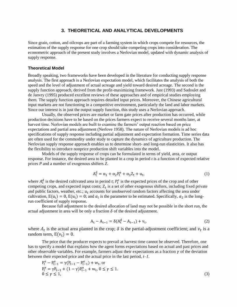
3. THEORETICAL AND ANALYTICAL DEVELOPMENTS

Since grain, cotton, and oilcrops are part of a farming system in which crops compete for resources, the

estimation of the supply response for one crop should take competing crops into consideration. The

econometric approach of the present study involves a Nerlovian model, updated with dynamic analysis of

supply response.

Theoretical Model

Broadly speaking, two frameworks have been developed in the literature for conducting supply response

analysis. The first approach is a Nerlovian expectation model, which facilitates the analysis of both the

speed and the level of adjustment of actual acreage and yield toward desired acreage. The second is the

supply function approach, derived from the profit-maximizing framework. Just (1993) and Sadoulet and

de Janvry (1995) produced excellent reviews of these approaches and of empirical studies employing

them. The supply function approach requires detailed input prices. Moreover, the Chinese agricultural

input markets are not functioning in a competitive environment, particularly the land and labor markets.

Since our interest is in just the output supply function, this study uses a Nerlovian approach.

Usually, the observed prices are market or farm gate prices after production has occurred, while

production decisions have to be based on the prices farmers expect to receive several months later, at

harvest time. Nerlovian models are built to examine the farmers’ output reaction based on price

expectations and partial area adjustment (Nerlove 1958). The nature of Nerlovian models is ad hoc

specifications of supply response including partial adjustment and expectation formation. Time series data

are often used for the commodity under study to capture the dynamics of agriculture production. The

Nerlovian supply response approach enables us to determine short- and long-run elasticities. It also has

the flexibility to introduce nonprice production shift variables into the model.

Models of the supply response of crops can be formulated in terms of yield, area, or output

response. For instance, the desired area to be planted in a crop in period t is a function of expected relative

prices P and a number of exogenous shifters Z.

, (1)

where is the desired cultivated area in period t; is the expected prices of the crop and of other

competing crops, and expected input costs; is a set of other exogenous shifters, including fixed private

and public factors, weather, etc.; accounts for unobserved random factors affecting the area under

cultivation, , ; and is the parameter to be estimated. Specifically, is the long-

run coefficient of supply response.

Because full adjustment to the desired allocation of land may not be possible in the short run, the

actual adjustment in area will be only a fraction of the desired adjustment.

. (2)

where is the actual area planted in the crop; is the partial-adjustment coefficient; and is a

random term, .

The price that the producer expects to prevail at harvest time cannot be observed. Therefore, one

has to specify a model that explains how the agent forms expectations based on actual and past prices and

other observable variables. For example, farmers adjust their expectations as a fraction of the deviation

between their expected price and the actual price in the last period, t–1.

, or

, .

, (3)

2

where is the expected price for period t; is the price that prevails when decisionmaking for

production in period t occurs; is the adaptive-expectations coefficient; and is a random term,

.

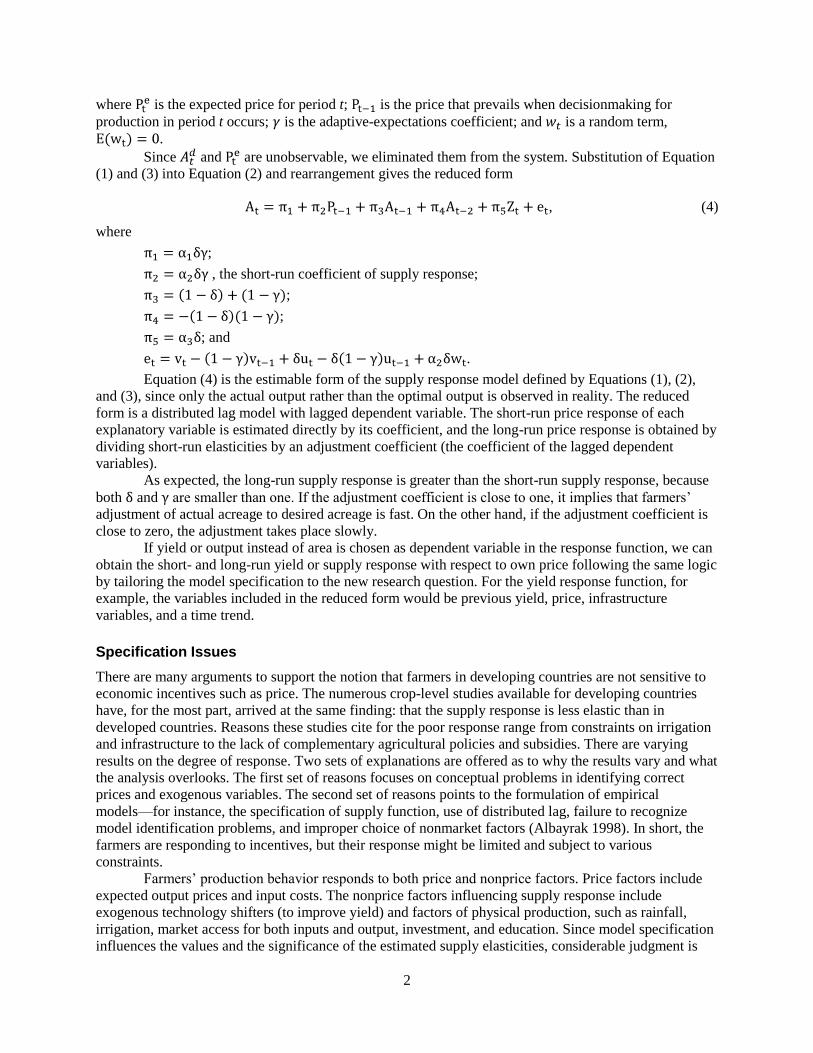
Since and are unobservable, we eliminated them from the system. Substitution of Equation

(1) and (3) into Equation (2) and rearrangement gives the reduced form

, (4)

where

;

, the short-run coefficient of supply response;

;

;

; and

.

Equation (4) is the estimable form of the supply response model defined by Equations (1), (2),

and (3), since only the actual output rather than the optimal output is observed in reality. The reduced

form is a distributed lag model with lagged dependent variable. The short-run price response of each

explanatory variable is estimated directly by its coefficient, and the long-run price response is obtained by

dividing short-run elasticities by an adjustment coefficient (the coefficient of the lagged dependent

variables).

As expected, the long-run supply response is greater than the short-run supply response, because

both and are smaller than one. If the adjustment coefficient is close to one, it implies that farmers’

adjustment of actual acreage to desired acreage is fast. On the other hand, if the adjustment coefficient is

close to zero, the adjustment takes place slowly.

If yield or output instead of area is chosen as dependent variable in the response function, we can

obtain the short- and long-run yield or supply response with respect to own price following the same logic

by tailoring the model specification to the new research question. For the yield response function, for

example, the variables included in the reduced form would be previous yield, price, infrastructure

variables, and a time trend.

Specification Issues

There are many arguments to support the notion that farmers in developing countries are not sensitive to

economic incentives such as price. The numerous crop-level studies available for developing countries

have, for the most part, arrived at the same finding: that the supply response is less elastic than in

developed countries. Reasons these studies cite for the poor response range from constraints on irrigation

and infrastructure to the lack of complementary agricultural policies and subsidies. There are varying

results on the degree of response. Two sets of explanations are offered as to why the results vary and what

the analysis overlooks. The first set of reasons focuses on conceptual problems in identifying correct

prices and exogenous variables. The second set of reasons points to the formulation of empirical

models—for instance, the specification of supply function, use of distributed lag, failure to recognize

model identification problems, and improper choice of nonmarket factors (Albayrak 1998). In short, the

farmers are responding to incentives, but their response might be limited and subject to various

constraints.

Farmers’ production behavior responds to both price and nonprice factors. Price factors include

expected output prices and input costs. The nonprice factors influencing supply response include

exogenous technology shifters (to improve yield) and factors of physical production, such as rainfall,

irrigation, market access for both inputs and output, investment, and education. Since model specification

influences the values and the significance of the estimated supply elasticities, considerable judgment is

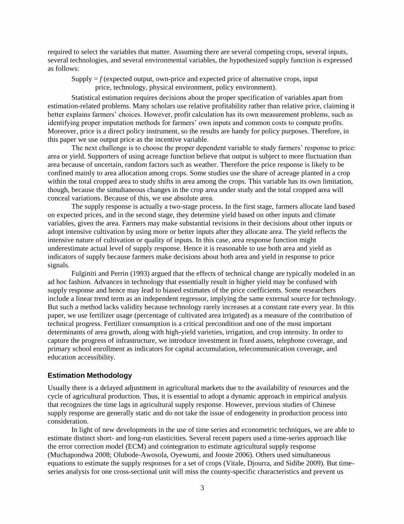
3

required to select the variables that matter. Assuming there are several competing crops, several inputs,

several technologies, and several environmental variables, the hypothesized supply function is expressed

as follows:

Supply = f (expected output, own-price and expected price of alternative crops, input

price, technology, physical environment, policy environment).

Statistical estimation requires decisions about the proper specification of variables apart from

estimation-related problems. Many scholars use relative profitability rather than relative price, claiming it

better explains farmers’ choices. However, profit calculation has its own measurement problems, such as

identifying proper imputation methods for farmers’ own inputs and common costs to compute profits.

Moreover, price is a direct policy instrument, so the results are handy for policy purposes. Therefore, in

this paper we use output price as the incentive variable.

The next challenge is to choose the proper dependent variable to study farmers’ response to price:

area or yield. Supporters of using acreage function believe that output is subject to more fluctuation than

area because of uncertain, random factors such as weather. Therefore the price response is likely to be

confined mainly to area allocation among crops. Some studies use the share of acreage planted in a crop

within the total cropped area to study shifts in area among the crops. This variable has its own limitation,

though, because the simultaneous changes in the crop area under study and the total cropped area will

conceal variations. Because of this, we use absolute area.

The supply response is actually a two-stage process. In the first stage, farmers allocate land based

on expected prices, and in the second stage, they determine yield based on other inputs and climate

variables, given the area. Farmers may make substantial revisions in their decisions about other inputs or

adopt intensive cultivation by using more or better inputs after they allocate area. The yield reflects the

intensive nature of cultivation or quality of inputs. In this case, area response function might

underestimate actual level of supply response. Hence it is reasonable to use both area and yield as

indicators of supply because farmers make decisions about both area and yield in response to price

signals.

Fulginiti and Perrin (1993) argued that the effects of technical change are typically modeled in an

ad hoc fashion. Advances in technology that essentially result in higher yield may be confused with

supply response and hence may lead to biased estimates of the price coefficients. Some researchers

include a linear trend term as an independent regressor, implying the same external source for technology.

But such a method lacks validity because technology rarely increases at a constant rate every year. In this

paper, we use fertilizer usage (percentage of cultivated area irrigated) as a measure of the contribution of

technical progress. Fertilizer consumption is a critical precondition and one of the most important

determinants of area growth, along with high-yield varieties, irrigation, and crop intensity. In order to

capture the progress of infrastructure, we introduce investment in fixed assets, telephone coverage, and

primary school enrollment as indicators for capital accumulation, telecommunication coverage, and

education accessibility.

Estimation Methodology

Usually there is a delayed adjustment in agricultural markets due to the availability of resources and the

cycle of agricultural production. Thus, it is essential to adopt a dynamic approach in empirical analysis

that recognizes the time lags in agricultural supply response. However, previous studies of Chinese

supply response are generally static and do not take the issue of endogeneity in production process into

consideration.

In light of new developments in the use of time series and econometric techniques, we are able to

estimate distinct short- and long-run elasticities. Several recent papers used a time-series approach like

the error correction model (ECM) and cointegration to estimate agricultural supply response

(Muchapondwa 2008; Olubode-Awosola, Oyewumi, and Jooste 2006). Others used simultaneous

equations to estimate the supply responses for a set of crops (Vitale, Djourra, and Sidibe 2009). But time-

series analysis for one cross-sectional unit will miss the county-specific characteristics and prevent us

4

from providing better information that can be used to draw inferences at the county level. In contrast,

panel data enable us to capture both regional and temporal variations in a dynamic fashion. This paper

estimates the supply response to price changes in three agricultural subsectors by applying dynamic panel

data techniques. Our methods employ sufficient information about the whole time period and individual

heterogeneity to investigate dynamic relationships and obtain consistent parameter estimates (Bond

2002).

Our methods account for both the simultaneity problem and the possibility of nonstationary

variables. First, the specified supply relationship implies that there is a unidirectional causality from

independent variables such as price to agricultural supply but not vice versa. In reality, it may well be the

case that price and supply are determined simultaneously, in which case estimates suffer from demand–

supply simultaneity bias. In the case of grain, such as maize and other coarse grain, the price of wheat in

Henan province is likely exogenous. That is because the Henan price depends on the national price and

production, and the latter do not necessarily depend on Henan’s production. Nevertheless, the price of

wheat in Henan is probably endogenous because the province’s share of national production is

substantial. Failure to deal properly with the simultaneity problem gives rise to inconsistent estimates.

Second, any variable series included in the analysis might not be stationary, that is, unit roots

exist. In this study, a generalized method of moments (GMM) estimator is used to gauge the supply

response function based on a dynamic panel data model, taking both endogeneity and dynamic panel bias

into consideration.

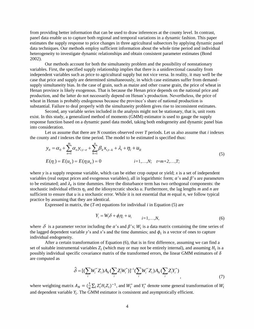
Let us assume that there are N counties observed over T periods. Let us also assume that i indexes

the county and t indexes the time period. The model to be estimated is specified thus:

,0 ,1 1

m n

it e i t e tk i t ke k

i ity y x u

(5)

( ) ( ) ( ) 0i it i itE E u E u i=1,…,N; t=m+2,…,T;

where y is a supply response variable, which can be either crop output or yield; x is a set of independent

variables (real output prices and exogenous variables), all in logarithmic form; ’s and ’s are parameters

to be estimated; and is time dummies. Here the disturbance term has two orthogonal components: the

stochastic individual effects and the idiosyncratic shocks u. Furthermore, the lag lengths m and n are

sufficient to ensure that u is a stochastic error. While it is not essential that m equal n, we follow typical

practice by assuming that they are identical.

Expressed in matrix, the (T-m) equations for individual i in Equation (5) are

i i i i iY W u i=1,…,N, (6)

where is a parameter vector including the ’s and ’s; is a data matrix containing the time series of

the lagged dependent variable y’s and x’s and the time dummies; and is a vector of ones to capture

individual endogeneity.

After a certain transformation of Equation (6), that is in first difference, assuming we can find a

set of suitable instrumental variables (which may or may not be entirely internal), and assuming is a

possibly individual specific covariance matrix of the transformed errors, the linear GMM estimators of

are computed as

*' ' * 1 *' ' *[( ) ( )] ( ) ( )i i N i i i i N i i

i i i i

W Z A Z W W Z A Z Y , (7)

where weighting matrix , and and denote some general transformation of

and dependent variable . The GMM estimator is consistent and asymptotically efficient.

5

The lagged dependent variables are endogenous to the individual effects in the error term in

Equation (7), causing dynamic panel bias. Arellano and Bond (1991) proposed a method to estimate a

dynamic panel difference model using all suitably lagged endogenous (and predetermined) variables as

instruments in the GMM technique, called difference GMM. In principle, efficient GMM exploits a

different number of instruments in each time period. Difference GMM avoids the trade-off between

instrument lag depth and sample depth in 2SLS by including separate instruments for each time period.

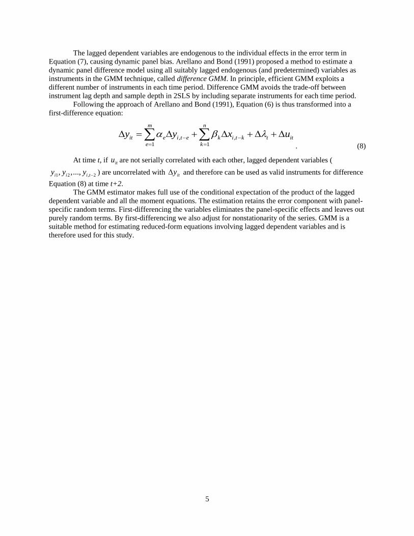
Following the approach of Arellano and Bond (1991), Equation (6) is thus transformed into a

first-difference equation:

, ,

1 1

m n

it e i t e k i t k t it

e k

y y x u

. (8)

At time t, if itu are not serially correlated with each other, lagged dependent variables (

1 2 , 2, ,...,i i i ty y y ) are uncorrelated with ity and therefore can be used as valid instruments for difference

Equation (8) at time t+2.

The GMM estimator makes full use of the conditional expectation of the product of the lagged

dependent variable and all the moment equations. The estimation retains the error component with panel-

specific random terms. First-differencing the variables eliminates the panel-specific effects and leaves out

purely random terms. By first-differencing we also adjust for nonstationarity of the series. GMM is a

suitable method for estimating reduced-form equations involving lagged dependent variables and is

therefore used for this study.

6

4. DATA AND VARIABLES

We obtained the county-level area, yield, and other related variables for 1998–2007 from Henan

statistical yearbook (various years). There are 109 counties in the province, but Jiyuan was dropped due

to data constraint. Among the remaining 108 counties, 66 are in the flat Plain zone, 26 in the Hill zone

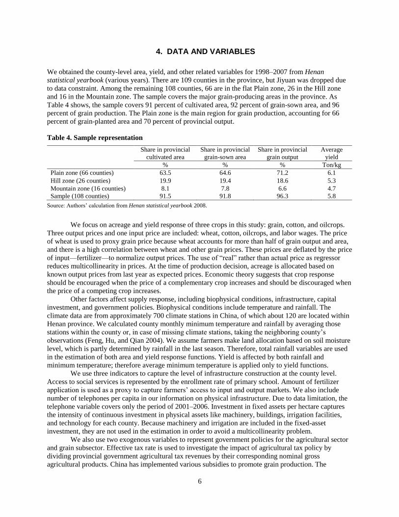
and 16 in the Mountain zone. The sample covers the major grain-producing areas in the province. As

Table 4 shows, the sample covers 91 percent of cultivated area, 92 percent of grain-sown area, and 96

percent of grain production. The Plain zone is the main region for grain production, accounting for 66

percent of grain-planted area and 70 percent of provincial output.

Table 4. Sample representation

Share in provincial

cultivated area

Share in provincial

grain-sown area

Share in provincial

grain output

Average

yield

% % % Ton/kg

Plain zone (66 counties) 63.5 64.6 71.2 6.1

Hill zone (26 counties) 19.9 19.4 18.6 5.3

Mountain zone (16 counties) 8.1 7.8 6.6 4.7

Sample (108 counties) 91.5 91.8 96.3 5.8

Source: Authors’ calculation from Henan statistical yearbook 2008.

We focus on acreage and yield response of three crops in this study: grain, cotton, and oilcrops.

Three output prices and one input price are included: wheat, cotton, oilcrops, and labor wages. The price

of wheat is used to proxy grain price because wheat accounts for more than half of grain output and area,

and there is a high correlation between wheat and other grain prices. These prices are deflated by the price

of input—fertilizer—to normalize output prices. The use of ―real‖ rather than actual price as regressor

reduces multicollinearity in prices. At the time of production decision, acreage is allocated based on

known output prices from last year as expected prices. Economic theory suggests that crop response

should be encouraged when the price of a complementary crop increases and should be discouraged when

the price of a competing crop increases.

Other factors affect supply response, including biophysical conditions, infrastructure, capital

investment, and government policies. Biophysical conditions include temperature and rainfall. The

climate data are from approximately 700 climate stations in China, of which about 120 are located within

Henan province. We calculated county monthly minimum temperature and rainfall by averaging those

stations within the county or, in case of missing climate stations, taking the neighboring county’s

observations (Feng, Hu, and Qian 2004). We assume farmers make land allocation based on soil moisture

level, which is partly determined by rainfall in the last season. Therefore, total rainfall variables are used

in the estimation of both area and yield response functions. Yield is affected by both rainfall and

minimum temperature; therefore average minimum temperature is applied only to yield functions.

We use three indicators to capture the level of infrastructure construction at the county level.

Access to social services is represented by the enrollment rate of primary school. Amount of fertilizer

application is used as a proxy to capture farmers’ access to input and output markets. We also include

number of telephones per capita in our information on physical infrastructure. Due to data limitation, the

telephone variable covers only the period of 2001–2006. Investment in fixed assets per hectare captures

the intensity of continuous investment in physical assets like machinery, buildings, irrigation facilities,

and technology for each county. Because machinery and irrigation are included in the fixed-asset

investment, they are not used in the estimation in order to avoid a multicollinearity problem.

We also use two exogenous variables to represent government policies for the agricultural sector

and grain subsector. Effective tax rate is used to investigate the impact of agricultural tax policy by

dividing provincial government agricultural tax revenues by their corresponding nominal gross

agricultural products. China has implemented various subsidies to promote grain production. The

7

provincial-level grain subsidy, set in 2004, is also included in the study to quantify the impact of grain

subsidy on the responsiveness of grain and non-grain crops. We expect the signs of all the variables to be

positive except for tax rate.

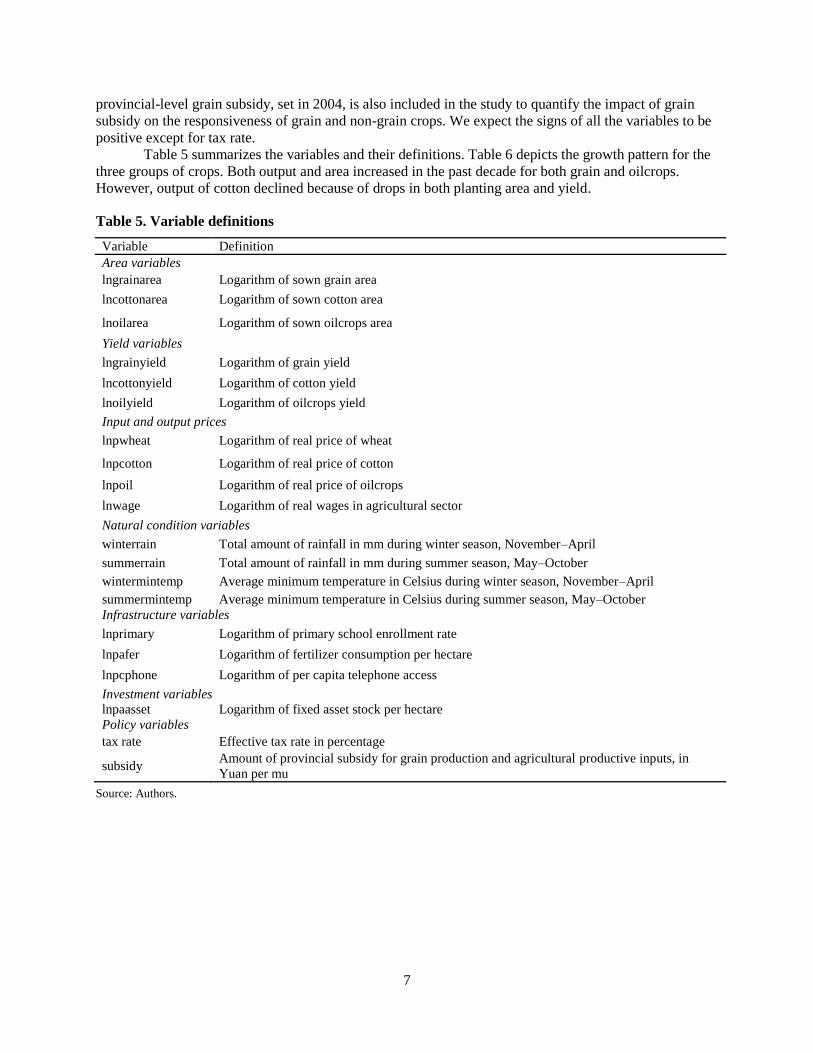
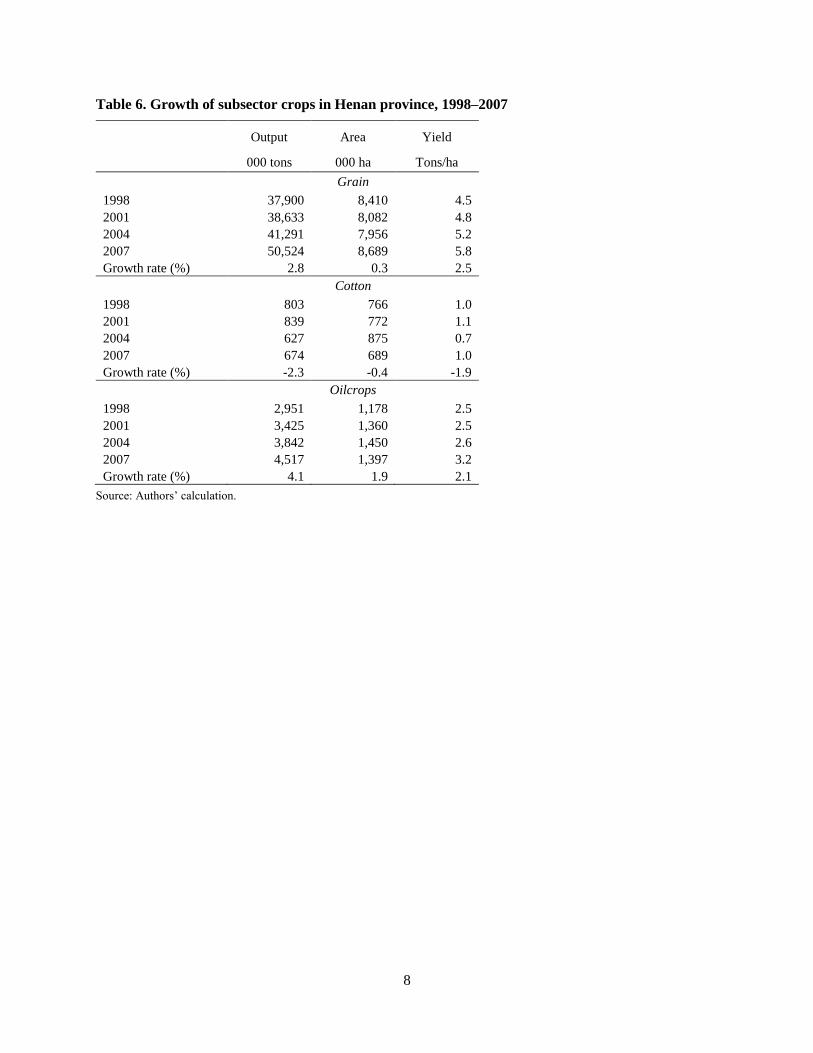
Table 5 summarizes the variables and their definitions. Table 6 depicts the growth pattern for the

three groups of crops. Both output and area increased in the past decade for both grain and oilcrops.

However, output of cotton declined because of drops in both planting area and yield.

Table 5. Variable definitions

Variable Definition

Area variables

lngrainarea Logarithm of sown grain area

lncottonarea Logarithm of sown cotton area

lnoilarea Logarithm of sown oilcrops area

Yield variables

lngrainyield Logarithm of grain yield

lncottonyield Logarithm of cotton yield

lnoilyield Logarithm of oilcrops yield

Input and output prices

lnpwheat Logarithm of real price of wheat

lnpcotton Logarithm of real price of cotton

lnpoil Logarithm of real price of oilcrops

lnwage Logarithm of real wages in agricultural sector

Natural condition variables

winterrain Total amount of rainfall in mm during winter season, November–April

summerrain Total amount of rainfall in mm during summer season, May–October

wintermintemp Average minimum temperature in Celsius during winter season, November–April

summermintemp Average minimum temperature in Celsius during summer season, May–October

Infrastructure variables

lnprimary Logarithm of primary school enrollment rate

lnpafer Logarithm of fertilizer consumption per hectare

lnpcphone Logarithm of per capita telephone access

Investment variables

lnpaasset Logarithm of fixed asset stock per hectare

Policy variables

tax rate Effective tax rate in percentage

subsidy Amount of provincial subsidy for grain production and agricultural productive inputs, in

Yuan per mu

Source: Authors.

8

Table 6. Growth of subsector crops in Henan province, 1998–2007

Output Area Yield

000 tons 000 ha Tons/ha

Grain

1998 37,900 8,410 4.5

2001 38,633 8,082 4.8

2004 41,291 7,956 5.2

2007 50,524 8,689 5.8

Growth rate (%) 2.8 0.3 2.5

Cotton

1998 803 766 1.0

2001 839 772 1.1

2004 627 875 0.7

2007 674 689 1.0

Growth rate (%) -2.3 -0.4 -1.9

Oilcrops

1998 2,951 1,178 2.5

2001 3,425 1,360 2.5

2004 3,842 1,450 2.6

2007 4,517 1,397 3.2

Growth rate (%) 4.1 1.9 2.1

Source: Authors’ calculation.

9

5. EMPIRICAL ANALYSIS OF ACREAGE, YIELD, AND SUPPLY RESPONSE

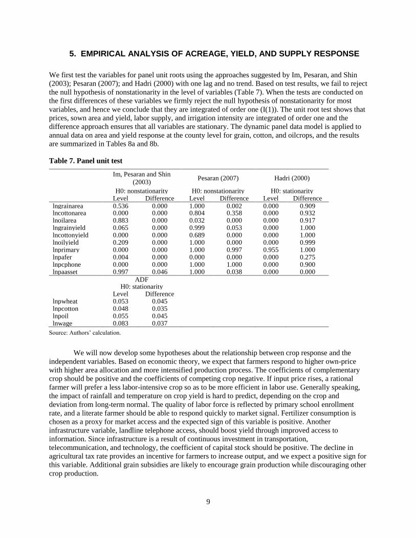
We first test the variables for panel unit roots using the approaches suggested by Im, Pesaran, and Shin

(2003); Pesaran (2007); and Hadri (2000) with one lag and no trend. Based on test results, we fail to reject

the null hypothesis of nonstationarity in the level of variables (Table 7). When the tests are conducted on

the first differences of these variables we firmly reject the null hypothesis of nonstationarity for most

variables, and hence we conclude that they are integrated of order one (I(1)). The unit root test shows that

prices, sown area and yield, labor supply, and irrigation intensity are integrated of order one and the

difference approach ensures that all variables are stationary. The dynamic panel data model is applied to

annual data on area and yield response at the county level for grain, cotton, and oilcrops, and the results

are summarized in Tables 8a and 8b.

Table 7. Panel unit test

Im, Pesaran and Shin

(2003) Pesaran (2007) Hadri (2000)

H0: nonstationarity H0: nonstationarity H0: stationarity Level Difference Level Difference Level Difference lngrainarea 0.536 0.000 1.000 0.002 0.000 0.909 lncottonarea 0.000 0.000 0.804 0.358 0.000 0.932 lnoilarea 0.883 0.000 0.032 0.000 0.000 0.917 lngrainyield 0.065 0.000 0.999 0.053 0.000 1.000 lncottonyield 0.000 0.000 0.689 0.000 0.000 1.000 lnoilyield 0.209 0.000 1.000 0.000 0.000 0.999 lnprimary 0.000 0.000 1.000 0.997 0.955 1.000 lnpafer 0.004 0.000 0.000 0.000 0.000 0.275 lnpcphone 0.000 0.000 1.000 1.000 0.000 0.900 lnpaasset 0.997 0.046 1.000 0.038 0.000 0.000

ADF H0: stationarity Level Difference lnpwheat 0.053 0.045 lnpcotton 0.048 0.035 lnpoil 0.055 0.045 lnwage 0.083 0.037


We will now develop some hypotheses about the relationship between crop response and the

independent variables. Based on economic theory, we expect that farmers respond to higher own-price

with higher area allocation and more intensified production process. The coefficients of complementary

crop should be positive and the coefficients of competing crop negative. If input price rises, a rational

farmer will prefer a less labor-intensive crop so as to be more efficient in labor use. Generally speaking,

the impact of rainfall and temperature on crop yield is hard to predict, depending on the crop and

deviation from long-term normal. The quality of labor force is reflected by primary school enrollment

rate, and a literate farmer should be able to respond quickly to market signal. Fertilizer consumption is

chosen as a proxy for market access and the expected sign of this variable is positive. Another

infrastructure variable, landline telephone access, should boost yield through improved access to

information. Since infrastructure is a result of continuous investment in transportation,

telecommunication, and technology, the coefficient of capital stock should be positive. The decline in

agricultural tax rate provides an incentive for farmers to increase output, and we expect a positive sign for

this variable. Additional grain subsidies are likely to encourage grain production while discouraging other

crop production.

10

Table 8a. Area and yield response in Henan province, 1998–2007

Area Response Yield Response

lngrainarea lncottonarea lnoilarea lngrainyield lncottonyield lnoilyield

dependent variable (-1) 0.661 0.019 0.374 -0.004 0.090 0.042

(7.65)*** (0.22) (4.54)*** (-0.09) (1.74)* (0.89)


lnpwheat (-1) 0.274 0.669 0.036 0.261

(4.57)*** (1.52) (0.25) (4.12)***

lnpcotton (-1) -0.036 0.738 -0.052 1.136

(-1.15) (2.77)*** (-0.75) (5.09)***

lnpoil (-1) -0.197 -1.002 -0.024 0.783

(-2.90)*** (-1.65)* (-0.14) (4.46)***

lnwage (-1) -0.081 -0.322 0.317 0.228 1.628 0.869

(-2.89)*** (-1.27) (3.73)*** (3.41)*** (5.72)*** (5.61)***


summerrain 0.000 -0.008 -0.001 0.000 0.014 -0.003

(0.75) (-1.78)* (-0.73) (0.29) (4.28)*** (-2.53)**

winterrain -0.000 -0.005 -0.006 -0.001 0.020 -0.008

(-0.11) (-0.60) (-2.39)** (-0.47) (2.15)** (-1.29)

summermintemp -0.008 -0.032 -0.009

(-1.74)* (-2.46)** (-0.87)

wintermintemp 0.016 0.365 0.052

(2.36)** (6.14)*** (4.03)***


lnprimary 0.255 -0.231 0.305 -0.024 3.480 1.265

(0.84) (-0.14) (0.39) (-0.04) (1.77)* (1.00)

lnpafer -0.008 0.021 0.061 -0.018 0.091 0.011

(-0.74) (0.40) (2.39)** (-0.56) (0.98) (0.19)


lnpaasset (-1) 0.088 0.304 -0.013 -0.100 -0.322 -0.153

(5.32)*** (2.71)*** (-0.37) (-2.35)** (-2.93)*** (-1.59)

Policy variables

tax rate -0.003 -0.026 -0.017 -0.038 -0.219 -0.077

(-0.41) (-0.31) (-0.87) (-3.23)*** (-5.84)*** (-3.25)***

subsidy -0.013 -0.090 -0.017 0.027 -0.132 0.020

(-2.93)*** (-2.33)** (-1.84)* (4.38)*** (-4.55)*** (1.40)

Constant 0.418 2.067 -1.992 1.118 -17.051 -0.440

(0.27) (0.28) (-0.56) (0.36) (-1.78)* (-0.07)

AR(1) 0.000 0.000 0.000 0.000 0.000 0.000

AR(2) 0.333 0.138 0.258 0.563 0.983 0.921

P-value of Sargan

exogeneity test 0.009 0.000 0.000 0.000 0.000 0.000

Observations 972 954 972 972 954 972

Number of counties 108 106 108 108 106 108


Note: Z-statistics in parentheses, *** p<0.01, ** p<0.05, * p<0.1.

11

Table 8b. Area and yield response in Henan province with telephone access, 2001–2006


lngrainarea lncottonarea lnoilarea lngrainyield lncottonyield lnoilyield

dependent variable (-1) 0.537 0.035 0.452 -0.129 -0.074 -0.004

(3.42)*** (0.34) (4.62)*** (-1.54) (-0.70) (-0.05)


lnpwheat (-1) 0.339 -0.496 -0.023 -0.025 0.315 -0.602

(2.02)** (-0.70) (-0.09) (-0.22) (1.46) (-1.52)

lnpcotton (-1) 0.063 2.034 -0.165

(0.74) (5.33)*** (-1.53)

lnpoil (-1) -0.179 0.058 0.127

(-1.47) (0.12) (0.70)

lnwage (-1) -0.629 -3.777 0.234 0.281 -2.183 0.799

(-2.64)*** (-4.16)*** (0.77) (0.75) (-2.06)** (0.97)


summerrain -0.001 -0.020 0.002 -0.001 0.005 0.005

(-1.30) (-4.29)*** (1.33) (-0.33) (0.87) (1.23)

winterrain 0.010 0.017 -0.002 -0.022 0.033 -0.052

(2.06)** (0.86) (-0.38) (-2.90)*** (1.13) (-3.09)***

summermintemp 0.010 -0.056 0.081

(0.39) (-0.75) (1.33)

wintermintemp 0.011 0.287 0.113

(0.66) (3.51)*** (2.95)***


lnprimary -0.209 -1.078 1.132 1.380 6.584 4.718

(-0.41) (-0.55) (1.25) (1.07) (1.83)* (1.81)*

lnpafer -0.019 -0.005 0.028 -0.117 -0.456 0.222

(-1.14) (-0.08) (0.96) (-1.08) (-1.88)* (1.52)

L.lnpcphone 0.248 0.130 -0.283 0.567 1.556 1.101

(2.93)*** (0.49) (-1.95)* (2.87)*** (2.38)** (2.32)**


lnpaasset (-1) 0.025 0.308 -0.017 -0.054 -0.540 -0.279

(1.09) (3.65)*** (-0.56) (-1.18) (-3.52)*** (-2.53)**

Constant 7.792 30.156 -5.776 -5.438 2.271 -13.392

(2.50)** (2.43)** (-1.12) (-0.80) (0.11) (-0.92)

AR(1) 0.000 0.000 0.000 0.000 0.000 0.000

AR(2) 0.268 0.674 0.814 0.364 0.044 0.979

P-value of Sargan

exogeneity test 0.998 0.249 0.002 0.000 0.000 0.021

Observations 648 636 648 648 636 648

Number of counties 108 106 108 108 106 108


Note: Z-statistics in parentheses, *** p<0.01, ** p<0.05, * p<0.1.

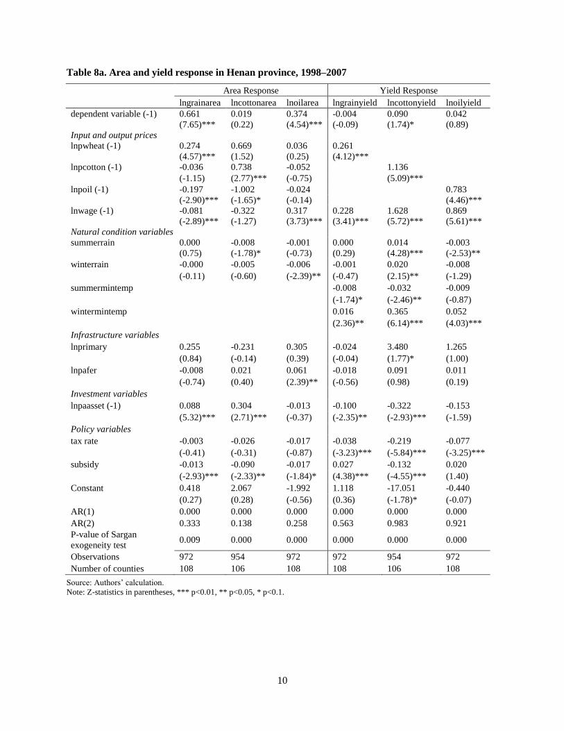
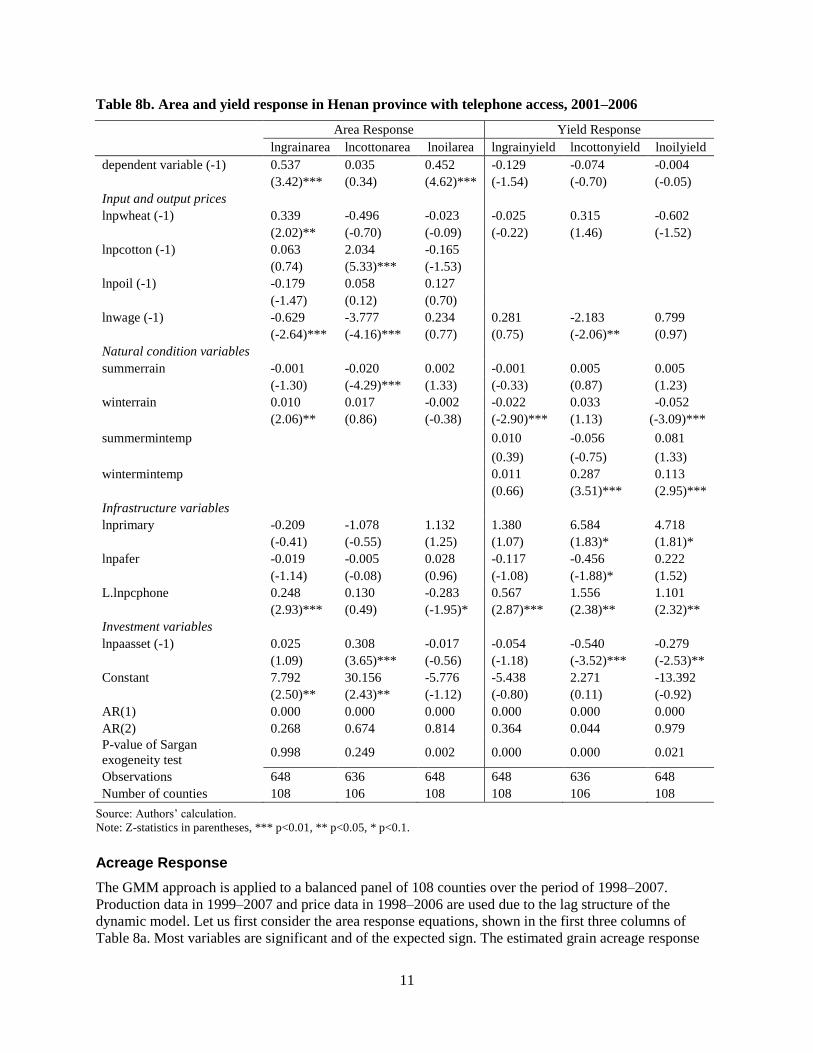
Acreage Response

The GMM approach is applied to a balanced panel of 108 counties over the period of 1998–2007.

Production data in 1999–2007 and price data in 1998–2006 are used due to the lag structure of the

dynamic model. Let us first consider the area response equations, shown in the first three columns of

Table 8a. Most variables are significant and of the expected sign. The estimated grain acreage response

12

model (in the first column) provides a good fit. The coefficients of the estimated parameters for the

response of grain to its own-price and to the price of oilcrops are significant and consistent with standard

production theory: a positive supply response to own-price and a negative response to competing crop

price. The results reveal that grain acreage is significantly influenced by the prices of wheat and oilcrops.

When the price of wheat rises by 1 percent, farmers choose to increase the share of their land allocated to

grain cultivation by 0.27 percent. When the price of oilcrops rises by 1 percent, farmers are likely to

decrease the land share they allocate to grain by 0.20 percent. The responses of cotton area (in the second

column) with respect to cotton and oilcrops prices are large, suggesting the land allocated for cotton

cultivation is more volatile than that of other crops, probably because cotton production is completely

market-oriented. Coefficients of prices for oilcrops acreage (third column) are not significant, indicating

that oilcrops are competing crops for grain but not vice versa, which is consistent with the crop calendar

(Meng et al. 2006). The acreage response of grain to real labor cost is negative and significant, while the

oilcrops acreage responds positively to higher labor cost. The results suggest that farmers choose to put

more labor into high-return oilcrops and less into grain as real wages increase.

We consider total rainfall from the previous growing season for both summer and winter crops.

Increased rainfall decreases the land cultivated under cotton and oilcrops. This is partly because cotton

and oilcrops are mostly grown in dry environments and excess soil moisture could hinder crop

production. Farmers therefore reduce the area devoted to cotton and oilcrops as a short-term strategy to

adapt to excess rainfall.

The indicator of education accessibility, enrollment rate in primary school, has a large but

insignificant coefficient, which is not surprising in the case of Henan. The province has achieved

universal primary education in more than half of its counties, so there is little heterogeneity in this

variable. Increasing fertilizer application by 1 percent could boost the cultivation area of oilcrops by 0.06

percent if everything else remains constant. Coefficients for investment in fixed assets are significant for

grain and cotton. Their positive signs agree with our expectation that an improved external environment

will facilitate farmers’ access to markets and adoption of modern technology, thereby improving supply

responsiveness through synergetic effects among factors influencing production process (seed, fertilizer,

and market information, among others). The results underscore the importance of infrastructure and

technology in improving crop yield.

Coefficients for the effective agricultural tax are negative but insignificant. The variable subsidy

captures the government’s support for grain production, and the coefficients are negative for all crops.

The negative responses of non-grain crops (cotton and oilcrops) at the increase of grain subsidy are as

expected, since grain subsidy discourages the allocation of resources to non-grain crops. However, the

negative coefficient of subsidy for grain area function suggests that subsidy does not increase area

devoted to grain production. In policy implementation, the exact amount of subsidies received by farmers

is based on the household’s total crop cultivation area instead of actual grain cultivation area. As a result,

grain subsidy becomes another form of income subsidy because the additional income is not directly

linked to farmers’ grain area allocation. Although the grain subsidy is intended to encourage grain

production, there is little evidence to suggest the policy achieves its purpose of encouraging farmers to

assign higher priority to grain crops.

Yield Response

Turning to the yield equations (the next three columns of Table 8a), we find that own-price response is

significant and positive for grain. When grain price increases by 1 percent, average grain yield increases

by 0.26 percent. The coefficients of own-price elasticities of the yield response functions of cotton and

oilcrops are positive and large, 1.14 for cotton and 0.78 for oilcrops, suggesting that yield of cash crops is

more responsive to price signals than is the yield of grain, which is consistent with our expectation. Yield

responds to labor wages positively, with the highest elasticity for cotton yield, at 1.63. The magnitude of

coefficients matches our expectations since grain is more mechanized and less labor-intensive than the

other crops. In contrast, cotton is handpicked, placing a high demand on labor. The positive signs of the

13

wage coefficients suggest that farmers are more efficient and more productive when the cost of hiring

labor rises.

Rainfall relates negatively to oilcrops yield but positively to cotton yield. We also considered

average winter and summer minimum temperature in the yield response to capture year-to-year variations

of exogenous climatic conditions. The coefficients for average summer minimum temperature are

negative in grain and cotton yield response functions. This is because a higher temperature during the

summer is harmful for crop growth. It also implies that global warming due to climate change would have

a negative impact on crop yield, consistent with many studies (You et al. 2009; Peng et al. 2004) On the

other hand, coefficients of winter minimum temperature are positive and significant for all crops,

suggesting that a rise in ground temperature could lift the yield of winter crops. Too-low temperature

during the winter would slow down the crop growth or even damage the crops.

Other nonprice, nonclimatic factors also contribute to yield response, and these include labor

quality and infrastructure. The coefficient for primary school enrollment is large and positive for cotton

yield function. Many researchers have argued that chemical fertilizer has been overused in China, causing

adverse environmental consequences without further improvement in productivity. Our results confirm

this observation: Fertilizer consumption intensity, a proxy for market access and technology, does not

demonstrate any positive influence on the yield. Although capital stock of fixed assets is negatively

associated with crop yield, we find it is positively correlated with crop area, with more or less similar

magnitude. This is probably attributable to an urban-biased investment strategy, which does not bring

growth in agricultural productivity despite fast growth in infrastructure such as transportation and

communication.

The declining agricultural tax generates coefficients with expected signs across all three groups.

When the agricultural tax rate drops by one percentage point, the average yield of grain and oilcrops

increases by 0.04 and 0.08 percent, respectively. Cotton farmers relieved from the heavier tax burden are

more productive, with a 0.22 percent increase in yield for each percentage point drop in tax rate. The

implementation of grain and comprehensive subsidies stimulate grain production but suppress cotton

production. If total subsidies for grain production increase by one Yuan per mu, average grain yield could

increase by 0.03 percent while cotton yield may drop by 0.13 percent.

Statistical Test and Regional Difference

Table 8b reports the area and yield responses correlated with telephone accessibility. The government

policy variables are dropped due to multicollinearity in the sample years of 2001–2006. The results are

similar to Table 8a but of different magnitude. Coefficients for telephone access are positive and

significant for all yield response functions. It is worth noting that average yield of cotton and oilcrops

could surge by 1.56 and 1.10 percent respectively when telephone availability increases by one

percentage point. When combined with grain area response, elasticity of grain output with respect to

telephone access is 0.81.

The GMM estimator is consistent only if there is no second-order serial correlation in the

idiosyncratic error term of the first-difference equations. Arellano and Bond (1991) developed a z-test for

serial correlation that would render some lags invalid as instruments. If the disturbances are not serially

correlated, there should be evidence of significant negative first-order autocorrelation in differenced

residuals and no evidence of second-order autocorrelation in the differenced residuals. As expected, the

output above presents strong evidence against the null hypothesis of zero autocorrelation in the first-

differenced errors at order 1, AR(1). If serial correlation in the first-differenced errors is found at an order

higher than 1, the moment conditions for estimation are not valid. The AR(2) test result presents no

significant evidence of serial correlation in the first-differenced errors at order 2 and thus indicates that

our GMM estimator is consistent.

The Nerlovian model can be criticized on the basis of misspecification since it omits other

important determinants of output such as infrastructure and government policy. In this study we estimate

an extension of the Nerlovian model, whereby external factors are incorporated. Indeed, the Sargan test

14

for the exclusion of these variables yields a significant chi-square in all equations in Tables 8a and 8b.

Hence we conclude that the above Nerlovian model is not misspecified.

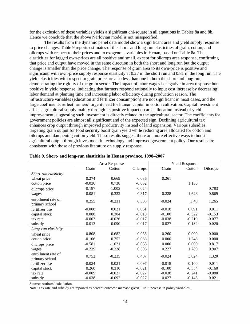
The results from the dynamic panel data model show a significant area and yield supply response

to price changes. Table 9 reports estimates of the short- and long-run elasticities of grain, cotton, and

oilcrops with respect to their prices and to exogenous variables in Henan, based on Table 8a. The

elasticities for lagged own-prices are all positive and small, except for oilcrops area response, confirming

that price and output have moved in the same direction in both the short and long run but the output

change is smaller than the price change. The response of grain area to its own-price is positive and

significant, with own-price supply response elasticity at 0.27 in the short run and 0.81 in the long run. The

yield elasticities with respect to grain price are also less than one in both the short and long run,

demonstrating the rigidity of the grain sector. The impact of labor wages is negative in area response but

positive in yield response, indicating that farmers respond rationally to input cost increase by decreasing

labor demand at planting time and increasing labor efficiency during production season. The

infrastructure variables (education and fertilizer consumption) are not significant in most cases, and the

large coefficients reflect farmers’ urgent need for human capital in cotton cultivation. Capital investment

affects agricultural supply mainly through its positive impact on area allocation instead of yield

improvement, suggesting such investment is directly related to the agricultural sector. The coefficients for

government policies are almost all significant and of the expected sign. Declining agricultural tax

enhances crop output through improved productivity instead of land expansion. Various subsidies

targeting grain output for food security boost grain yield while reducing area allocated for cotton and

oilcrops and dampening cotton yield. These results suggest there are more effective ways to boost

agricultural output through investment in technology and improved government policy. Our results are

consistent with those of previous literature on supply response.

Table 9. Short- and long-run elasticities in Henan province, 1998–2007


Grain Cotton Oilcrops Grain Cotton Oilcrops

Short-run elasticity

wheat price 0.274 0.669 0.036 0.261

cotton price -0.036 0.738 -0.052 1.136

oilcrops price -0.197 -1.002 -0.024 0.783

wages -0.081 -0.322 0.317 0.228 1.628 0.869

enrollment rate of

primary school 0.255 -0.231 0.305 -0.024 3.48 1.265

fertilizer use -0.008 0.021 0.061 -0.018 0.091 0.011

capital stock 0.088 0.304 -0.013 -0.100 -0.322 -0.153

tax rate -0.003 -0.026 -0.017 -0.038 -0.219 -0.077

subsidy -0.013 -0.090 -0.017 0.027 -0.132 0.020

Long-run elasticity

wheat price 0.808 0.682 0.058 0.260 0.000 0.000

cotton price -0.106 0.752 -0.083 0.000 1.248 0.000

oilcrops price -0.581 -1.021 -0.038 0.000 0.000 0.817

wages -0.239 -0.328 0.506 0.227 1.789 0.907

enrollment rate of

primary school 0.752 -0.235 0.487 -0.024 3.824 1.320

fertilizer use -0.024 0.021 0.097 -0.018 0.100 0.011

capital stock 0.260 0.310 -0.021 -0.100 -0.354 -0.160

tax rate -0.009 -0.027 -0.027 -0.038 -0.241 -0.080

subsidy -0.038 -0.092 -0.027 0.027 -0.145 0.021


Note: Tax rate and subsidy are reported as percent outcome increase given 1 unit increase in policy variables.

15

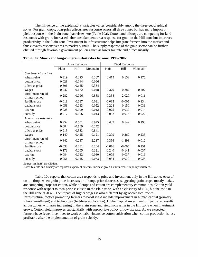
The influence of the explanatory variables varies considerably among the three geographical

zones. For grain crops, own-price affects area response across all three zones but has more impact on

yield response in the Plain zone than elsewhere (Table 10a). Cotton and oilcrops are competing for land

resources with grain. Increased labor cost dampens area response for grain in the Hill zone but improves

productivity in the Plain zone. Investment in infrastructure helps integrate farmers into the market and

thus elevates responsiveness to market signals. The supply response of the grain sector can be further

elicited through favorable government policies such as lower tax rate and direct subsidy.

Table 10a. Short- and long-run grain elasticities by zone, 1998–2007


Plain Hill Mountain Plain Hill Mountain

Short-run elasticities

wheat price 0.319 0.223 0.387 0.415 0.152 0.176

cotton price 0.028 -0.044 -0.096

oilcrops price -0.306 -0.155 -0.334

wages -0.047 -0.172 -0.048 0.379 -0.287 0.207

enrollment rate of

primary school 0.282 0.096 -0.888 0.338 -2.020 -0.011

fertilizer use -0.011 0.037 0.081 -0.015 -0.005 0.134

capital stock 0.058 0.083 0.052 -0.228 -0.150 -0.033

tax rate -0.028 0.009 -0.012 -0.075 -0.039 -0.014

subsidy -0.017 -0.006 -0.013 0.032 0.075 0.022

Long-run elasticities

wheat price 0.952 0.551 0.975 0.437 0.142 0.198

cotton price 0.084 -0.109 -0.242

oilcrops price -0.913 -0.383 -0.841

wages -0.140 -0.425 -0.121 0.399 -0.269 0.233

enrollment rate of

primary school 0.842 0.237 -2.237 0.356 -1.893 -0.012

fertilizer use -0.033 0.091 0.204 -0.016 -0.005 0.151

capital stock 0.173 0.205 0.131 -0.240 -0.141 -0.037

tax rate -0.084 0.022 -0.030 -0.079 -0.037 -0.016

subsidy -0.051 -0.015 -0.033 0.034 0.070 0.025



Table 10b reports that cotton area responds to price and investment only in the Hill zone. Area of

cotton drops when grain price increases or oilcrops price decreases, suggesting grain crops, mostly maize,

are competing crops for cotton, while oilcrops and cotton are complementary commodities. Cotton yield

response with respect to own-price is elastic in the Plain zone, with an elasticity of 1.05, but inelastic in

the Hill zone at -0.46. The impact of higher wages is also different by agroecological zones.

Infrastructural factors prompting farmers to boost yield include improvement in human capital (primary

school enrollment) and technology (fertilizer application). Higher capital investment brings mixed results

across zones, with area increasing in the Plain zone and yield increasing in the Hill zone when investment

grows. Cotton yield improves substantially with appropriate policy of low tax rate. As we expected,

farmers have fewer incentives to work on labor-intensive cotton cultivation when cotton production is less

profitable after the implementation of grain subsidy.

16

Table 10b. Short- and long-run cotton elasticities by zone, 1998–2007




wheat price 0.253 -1.707 -0.988

cotton price 0.309 -0.566 0.085 1.046 -0.457 -0.002

oilcrops price -0.134 2.288 0.219

wages -0.103 -0.412 0.529 2.072 -0.822 0.513

enrollment rate of

primary school 1.822 0.844 -1.038 4.065 -2.974 0.543

fertilizer use -0.001 0.036 0.495 0.038 0.925 0.167

capital stock 0.314 -0.242 -0.494 -0.412 0.325 -0.337

tax rate 0.102 0.221 -0.066 -0.250 0.091 -0.095

subsidy -0.051 0.158 0.067 -0.138 0.005 0.032


wheat price 0.228 -4.332 -1.217

cotton price 0.278 -1.437 0.105 1.072 -0.497 -0.002

oilcrops price -0.121 5.807 0.270

wages -0.093 -1.046 0.651 2.123 -0.893 0.431

enrollment rate of

primary school 1.640 2.142 -1.278 4.165 -3.233 0.457

fertilizer use -0.001 0.091 0.610 0.039 1.005 0.140

capital stock 0.283 -0.614 -0.608 -0.422 0.353 -0.283

tax rate 0.092 0.561 -0.081 -0.256 0.099 -0.080

subsidy -0.046 0.401 0.083 -0.141 0.005 0.027



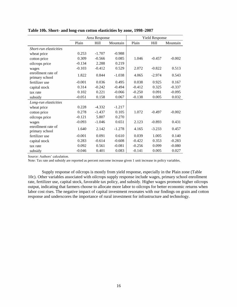
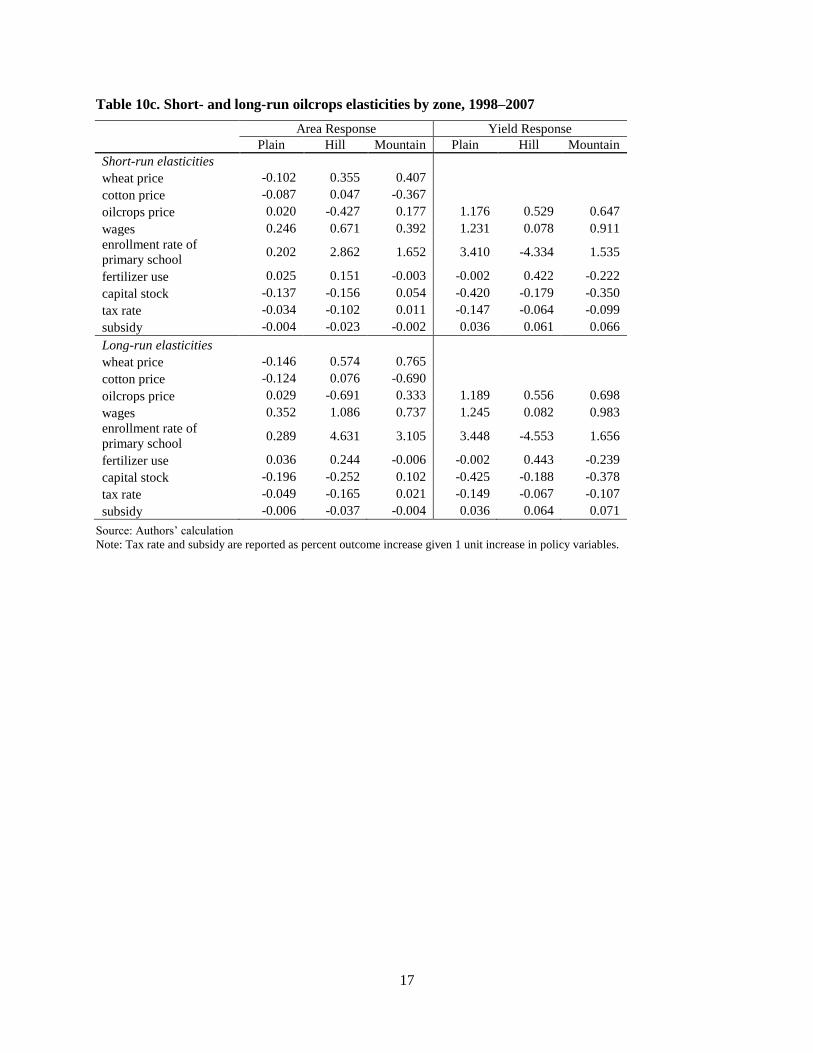
Supply response of oilcrops is mostly from yield response, especially in the Plain zone (Table

10c). Other variables associated with oilcrops supply response include wages, primary school enrollment

rate, fertilizer use, capital stock, favorable tax policy, and subsidy. Higher wages promote higher oilcrops

output, indicating that farmers choose to allocate more labor to oilcrops for better economic returns when

labor cost rises. The negative impact of capital investment resonates with our findings on grain and cotton

response and underscores the importance of rural investment for infrastructure and technology.

17

Table 10c. Short- and long-run oilcrops elasticities by zone, 1998–2007




wheat price -0.102 0.355 0.407

cotton price -0.087 0.047 -0.367

oilcrops price 0.020 -0.427 0.177 1.176 0.529 0.647

wages 0.246 0.671 0.392 1.231 0.078 0.911

enrollment rate of

primary school 0.202 2.862 1.652 3.410 -4.334 1.535

fertilizer use 0.025 0.151 -0.003 -0.002 0.422 -0.222

capital stock -0.137 -0.156 0.054 -0.420 -0.179 -0.350

tax rate -0.034 -0.102 0.011 -0.147 -0.064 -0.099

subsidy -0.004 -0.023 -0.002 0.036 0.061 0.066


wheat price -0.146 0.574 0.765

cotton price -0.124 0.076 -0.690

oilcrops price 0.029 -0.691 0.333 1.189 0.556 0.698

wages 0.352 1.086 0.737 1.245 0.082 0.983

enrollment rate of

primary school 0.289 4.631 3.105 3.448 -4.553 1.656

fertilizer use 0.036 0.244 -0.006 -0.002 0.443 -0.239

capital stock -0.196 -0.252 0.102 -0.425 -0.188 -0.378

tax rate -0.049 -0.165 0.021 -0.149 -0.067 -0.107

subsidy -0.006 -0.037 -0.004 0.036 0.064 0.071

Source: Authors’ calculation Note: Tax rate and subsidy are reported as percent outcome increase given 1 unit increase in policy variables.

18

6. CONCLUSION

The Chinese economy has undergone drastic transformation, characterized by rapid urbanization and

increased incomes. The extensive changes in economic and social structure require fast growth in the food

supply. Increasing the productivity of agriculture has been an important objective of the Chinese

government. Policy incentives, including tax decreases and subsidies, have been major policy instruments

to promote agricultural production. This paper reports the results of acreage and yield supply response

models fitted to a sample of 108 counties in one of the major agricultural provinces in China over the

1998–2007 period. The study estimates the agricultural supply response, taking into account the regime’s

policy change in China’s fast transformation. The dynamic panel data approach is appropriate to estimate

the short- and long-run relationship between agricultural supply and price while addressing the

endogeneity problems raised in earlier literature.

The major findings of this paper are, first, that crops area allocation is responsive to price

incentives in both short and long terms. The short-run elasticity for the county-level grain area planted,

with respect to own-price, is 0.27, and the corresponding long-run elasticity is 0.81. Future expansion of

grain output hinges on policies to improve relative price of grain or to reduce direct cost of grain

production, such as setting a minimum procurement price and providing input subsidies. Grain

responsiveness to output prices is greater than that to variable input price. This suggests that agricultural

policy should focus on output prices and input supply, such as access to credit and market, rather than on

input price per se. The recent grain policies by the Chinese government have had a positive effect on

grain output, and these policies include ensuring elimination of taxes and fees in the agricultural sector.

Second, there is still great potential to increase crop yield by improving infrastructure and social

services, including education, transportation, and communication. Our findings indicate that nonprice

factors are important means of affecting crop production and resource allocation, demonstrated by the

magnitudes of the elasticities of acreage and yield responses with respect to these factors. The most

important nonprice factors determining crop area are capital investment and fertilizer application. The

most important nonprice factor determining crop yield, and hence the major source of productivity

advance, is primary school enrollment. Given the high impact of school enrollment, investment in

improving labor quality still pays high dividends through increased productivity.

Third, government interventions need to emphasize more infrastructure construction in rural

areas, as suggested by the large and negative coefficients of investment variables for yield response.

Although acreage response to fixed-asset investment is positive, this effect is overshadowed by the larger

coefficients of yield response for grain and cotton. Further investment in machinery and transportation in

urban areas is unlikely to have an appreciable effect on crop yield, since productivity of the agricultural

sector benefits little if farmers are disconnected from technology and information.

Fourth, crop production response is substantially different under different government policies.

Subsidies for producing grain and purchasing input encourage farmers to improve grain yield. At the

same time, yields of non-grain crops suffer from the deteriorated terms of trade. Producers are motivated

to increase crop productivity when effective agricultural tax declines, due to decreased production cost. In

this context, the current agricultural policy of tax elimination and input subsidy is effective in increasing

crop productivity through proper incentives. However, it is worth noting that the subsidies do not achieve

the expected outcome of increasing grain cultivation area because in reality the subsidies are applied

universally to all crops instead of specifically targeting grain crops. Given the effectiveness of the subsidy

on grain yield response but ineffectiveness on area response, it is sensible to carefully evaluate the overall

effect of subsidy policies and design a comprehensive policy package to ensure long-term food security in

China.

Our results show that climate affects both crop production and farmers’ decisionmaking. Rising

temperature, due to climate change over the last few decades, has had a negative impact on crop yields. In

addition, as a short-term adaptation strategy, farmers use the previous season’s rainfall information and

seasonal climate forecasting to adjust the current season’s planting areas for different crops (grain, cotton,

19

oilcrops, and others). Future climate change would further raise the temperature and increase the

variability of factors such as rainfall in Henan and beyond. These results have valuable policy

implications in the formulation of climate change mitigation and adaptation strategies in China.

Government policy cannot affect natural conditions like rainfall and temperature, but it can compensate

for the negative impact of climate change by increasing investment in irrigation, promoting efficient use

of water, and encouraging adoption of drought-resistant varieties. Improving farmers’ access to seasonal

weather forecast information can be another tool of effective adaptation to climate change.

In summary, the Henan results indicate that Chinese agricultural policy should pay more attention

to technological advances and infrastructure improvements. Our findings suggest that China should

encourage modernization through investment in infrastructure, labor quality, and agricultural research and

development. Policy and public investments would help producers respond more flexibly to price shocks

and increase total supply. On the other hand, the effect of climate change on food security cannot be

ignored. Many measures can help farmers adapt to climate change. One is improved infrastructure and

labor quality as captured by the yield response model. Another measure is investment in agricultural

research and development to supply farmers with more drought- and flood-tolerant varieties as well as

more efficient production practices that are resilient in adverse soil and weather conditions. A

comprehensive package, including both agronomic and economic policies, is needed in the long run to

achieve the dual objectives of food security and income growth.

However, the promotion of modern technology and crop diversification should be tailored to local

conditions. The impact of public investment can be enhanced significantly if spatial variations are taken

into consideration at policy planning and implementation stages. In some regions with challenging

geographic conditions, such as the Mountain zone, poor infrastructure and poor information access

prevent local producers from benefiting from market conditions. Studies in many developing countries

indicate that investments in rural roads yield high returns in poverty reduction by improving rural access

to key services (Fan 2008). More investment in rural infrastructure could enable these farmers to collect

the latest market information and transport their produce to regional markets.

One limitation of this study is that it does not consider the improvement of grain crop varieties

over time, since improved variety is a major driver of crop productivity. It is estimated that new varieties

contributed to 20 percent of food crop production increase (Zhu 1997) and that 10 percent of wheat output

growth came from variety updating (Lou 2002). In recent years, dominant wheat varieties in Henan

province have evolved from high and steady yield to super-high yield, high quality, multi-resistance, and

extensive adaptability, ensuring a sustainable and stable growth of wheat yield (Song, Song, and Yin

2007). Meng et al. (2006) also reported that hybrid maize varieties dominated the whole Henan province

and no local varieties were cultivated because of the high yield from hybrid varieties. Although

information on grain variety remains scarce, it is probably safe to say that new varieties contribute

substantially to land productivity based on the historical trend.

20

REFERENCES

Albayrak, N. 1998. Wheat supply response: Some evidence on aggregation issues. Development Policy Review 16:

241–263.

Arellano, M., and S. Bond. 1991. Some tests of specification for panel data: Monte Carlo evidence and an

application to employment equations. Review of Economic Studies 58 (2): 277–297.

Binswanger, H. 1990. The policy response in agriculture. World Bank Research Observer 4: 231–258.

Bond, S. 2002. Dynamic panel data models: A guide to micro data methods and practice. Portuguese Economic

Journal 1 (2): 141–162.

Carter, C., and F. Zhong. 1988. China’s grain production and trade. Boulder, Colo.: Westview Press.

Chen, L., and A. Buckwell. 1991. Chinese grain economy and policy. Melksham, U.K.: Redwood Press.

China agroecological zones. 1985. Beijing, China: China Agriculture Press.

China statistical yearbook. 2008. Beijing: China Statistics Press.

Fan, S. 2008. Public expenditure, growth and poverty in developing countries: Issues, methods and findings.

Baltimore, Md.: Johns Hopkins Univ. Press.

Feng, S., Q. Hu, and W. Qian. 2004. Quality control of daily meterological data in China, 1951–2000: A new

dataset. International Journal of Climatology 24: 853–870.

Fulginiti, L., and R. Perrin. 1993. Prices and productivity in agriculture. Review of Economics and Statistics 75 (3):

471–482.

Hadri, K. 2000. Testing for stationarity in heterogeneous panel data. The Econometrics Journal 3: 148–161.

Henan statistical yearbook. Various years. Beijing: China Statistics Press.

Huang, Y. 1991. Estimating production interactions of agriculture in a semi-marketised economy: The case of

farming sector in China. Australia–Japan Research Center, the Australian National University, Canberra.

Mimeo.

Huang, J. and S. Rozelle. 1998b. Technological change, public investment, Institutional Innovation, and Grain

Production.‖ In China’s grain economy to the twenty-first century, eds. J. Huang and S. Rozelle. Beijing:

China Agriculture Press: 76.

Im, K. S., M. H. Pesaran, and Y. Shin. 2003. Testing for unit roots in heterogeneous panels. Journal of

Econometrics 115 (1): 53–74.

Just, R. E. 1993. Discovering production and supply relationships: Present status and future opportunities. Review of

Marketing and Agricultural Economics 61: 11–40.

Lin, J. 1992. Rural reform and agricultural growth in China. American Economic Review 82 (1): 34–51.

Lou, Y. 2002. Research on equilibrium between demand and supply and developing trend of wheat in China under

the layout of WTO. Journal of Agrotechnical Economics 6: 47-51.

Lu, W. 2002. Effects of agricultural market policy on crop production in China. Food Policy 27: 561–573.

Meng, E. C., R. Hu, X. Shi, and S. Zhang. 2006. Maize in China: Production systems, constraints, and research

priorities. Mexico, D.F.: International Maize and Wheat Improvement Center (CIMMYT). Ministry of

Finance of China.

<http://www.mof.gov.cn/mof/zhengwuxinxi/caizhengxinwen/200906/t20090626_172446.html>. Accessed

September, 2009.

Muchapondwa, E. 2008. Estimation of the aggregate agricultural supply response in Zimbabwe: The ARDL

approach to cointegration. Working Paper 90. Cape Town, S.A.: School of Economics, University of Cape

Town.

http://www.mof.gov.cn/mof/zhengwuxinxi/caizhengxinwen/200906/t20090626_172446.html

21

Mundlak, Y. 1985. The aggregate agricultural supply response. Working Paper 8511. Rehovot, Israel: Centre for

Agricultural Economic Research.

Nerlove, M. 1958. The dynamics of supply: Estimation of farmers’ response to price. Baltimore, Md.: Johns

Hopkins Univ. Press.

Olubode-Awosola, O., O. Oyewumi, and A. Jooste. 2006. Vector error correction modeling of Nigerian agricultural

supply response. Agrekon 45 (4): 421–432.

Peng, S., J. Huang, J. E. Sheehy, R. C. Laza, R. M. Visperas, X. Zhong, G. S. Centeno, G. S. Khush, and K. G.

Cassman. 2004. Rice yields decline with higher night temperature from global warming. The Proceedings

of National Academies of Science USA 101: 9971–9975.

Pesaran, M. H. 2007. A simple panel unit root test in the presence of cross section dependence. Journal of Applied

Econometrics 22: 265–312.

Sadoulet, E., and A. de Janvry. 1995. Quantitative development policy analysis. Baltimore, Md.: Johns Hopkins

Univ. Press.

Song, J., Y. Song, and J. Yin. 2007. Analysis on evolution of wheat variety in Henan. Chinese Business Review 6

(4): 61–64.

USDA (United States Department of Agriculture). 2000. Cross-commodity analysis of China’s grain sector: Sources

of growth and supply response. Market and Trade Economics Division Technical Bulletin 1884.

Washington, D.C.: Economic Research Service, USDA.

Vitale, J. D., H. Djourra, and A. Sidibe. 2009. Estimating the supply response of cotton and cereal crops in

smallholder production systems: Recent evidence from Mali. Agricultural Economics 40: 519–533.

World Bank. 1991. Options for reform in the grain sector. World Bank Country Study 9804. Washington, D.C.:

World Bank.

You, L., M. Rosegrant, S. Wood, and D. Sun. 2009. Impact of growing season temperature on wheat productivity in

China. Agricultural and Forest Meteorology 149 (6–7): 1009–1014.

Zhu, X. 1997. Exploration of new century: Research on food issue of China. Beijing: Chinese Agriculture Press.

RECENT IFPRI DISCUSSION PAPERS

For earlier discussion papers, please go to http://www.ifpri.org/publications/results/taxonomy%3A468. All discussion papers can be downloaded free of charge.

986. R&D investment in national and international agricultural research: An ex-ante analysis of productivity and poverty

impact. Alejandro Nin Pratt and Shenggen Fan, 2010

985. Food security and economic development in the Middle East and North Africa: Current state and future perspectives.

Clemens Breisinger, Teunis van Rheenen, Claudia Ringler, Alejandro Nin Pratt, Nicolas Minot, Catherine Aragon,

Bingxin Yu, Olivier Ecker, and Tingju Zhu, 2010.

984. Improving resource allocation and incomes in Vietnamese agriculture: A case study of farming in the Dong Nai River

Basin. Joshua Dewbre, 2010.

983. Positional spending and status seeking in rural China. Philip H. Brown, Erwin Bulte, and Xiaobo Zhang, 2010.

982. Assessing food security in Yemen: An innovative integrated, cross-sector, and multilevel approach. Olivier Ecker,

Clemens Breisinger, Christen McCool, Xinshen Diao, Jose Funes, Liangzhi You, and Bingxin Yu, 2010.

981. Long-term impact of investments in early schooling: Empirical evidence from rural Ethiopia. Subha Mani, John

Hoddinott, and John Strauss, 2010.

980. Infrastructure and cluster development: A case study of handloom weavers in Ethiopia. Gezahegn Ayele, Lisa Moorman,

Kassu Wamisho, and Xiaobo Zhang, 2010.

979. Country-level impact of global recession and China’s stimulus package: A general equilibrium assessment. Xinshen

Diao, Yumei Zhang, and Kevin Z. Chen, 2010.

978. Emergence of Sri Lanka in European fish trade: Is there cause for concern in the Lake Victoria Region (East Africa)?

Andrew Muhammad and Guyslain Ngeleza, 2010.

977. China has reached the Lewis Turning Point. Xiaobo Zhang, Jin Yang, and Shenglin Wang, 2010.

976. The medium-term impact of the primary education stipend in rural Bangladesh. Bob Baulch, 2010.

975. A review of empirical evidence on gender differences in nonland agricultural inputs, technology, and services in

developing countries. Amber Peterman, Julia Behrman, and Agnes Quisumbing, 2010.

974. An experiment on the impact of weather shocks and insurance on risky investment. Ruth Vargas Hill and Angelino

Viceisza, 2010.

973. Engendering agricultural research. Ruth Meinzen-Dick, Agnes Quisumbing, Julia Behrman, Patricia Biermayr-Jenzano,

Vicki Wilde, Marco Noordeloos, Catherine Ragasa, Nienke Beintema, 2010.

972. Sarpanch Raj: Is the president all powerful? The case of village councils in India. Nethra Palaniswamy, 2010.

971. Asset versus consumption poverty and poverty dynamics in the presence of multiple equilibria in rural Ethiopia. Lenis

Saweda O. Liverpool and Alex Winter-Nelson, 2010.

970. Poverty status and the impact of social networks on smallholder technology adoption in rural Ethiopia. Lenis Saweda O.

Liverpool and Alex Winter-Nelson, 2010.

969. Wage subsidies to combat unemployment and poverty: Assessing South Africa’s options. Justine Burns, Lawrence

Edwards, and Karl Pauw, 2010.

968. Patterns and trends of child and maternal nutrition inequalities in Nigeria. Babatunde Omilola, 2010.

967. Foreign inflows and growth challenges for African countries: An intertemporal general equilibrium assessment. Xinshen

Diao and Clemens Breisinger, 2010.

966. Biofuels and economic development in Tanzania. Channing Arndt, Karl Pauw, and James Thurlow, 2010.

965. Weathering the storm: Agricultural development, investment, and poverty in Africa following the recent food price crisis.

Babatunde Omilola and Melissa Lambert, 2010.

964. Who has influence in multistakeholder governance systems? Using the net-map method to analyze social networking in

watershed management in Northern Ghana. Eva Schiffer, Frank Hartwich, and Mario Monge, 2010.

http://www.ifpri.org/publications/results/taxonomy%3A468

INTERNATIONAL FOOD POLICY RESEARCH INSTITUTE

www.ifpri.org

IFPRI HEADQUARTERS

2033 K Street, NW Washington, DC 20006-1002 USA Tel.: +1-202-862-5600 Fax: +1-202-467-4439 Email: [email protected]

IFPRI ADDIS ABABA

P. O. Box 5689 Addis Ababa, Ethiopia Tel.: +251 11 6463215 Fax: +251 11 6462927 Email: [email protected]

IFPRI NEW DELHI

CG Block, NASC Complex, PUSA New Delhi 110-012 India Tel.: 91 11 2584-6565 Fax: 91 11 2584-8008 / 2584-6572 Email: [email protected]


Dynamic Agricultural Supply Response Under Economic Transformation: A Case Study of Henan, China

Documents