Durham E-Theses - CiteSeerX

Durham E-Theses

Biological studies on a number of Moorland Tipulidae

Butter�eld, J. E. L.

How to cite:

Butter�eld, J. E. L. (1973) Biological studies on a number of Moorland Tipulidae, Durham theses, DurhamUniversity. Available at Durham E-Theses Online: http://etheses.dur.ac.uk/8349/

Use policy

The full-text may be used and/or reproduced, and given to third parties in any format or medium, without prior permission orcharge, for personal research or study, educational, or not-for-pro�t purposes provided that:

• a full bibliographic reference is made to the original source

• a link is made to the metadata record in Durham E-Theses

• the full-text is not changed in any way

The full-text must not be sold in any format or medium without the formal permission of the copyright holders.

Please consult the full Durham E-Theses policy for further details.

Academic Support O�ce, Durham University, University O�ce, Old Elvet, Durham DH1 3HPe-mail: [email protected] Tel: +44 0191 334 6107

http://etheses.dur.ac.uk

Biological studies on a number of 1aoorland Tipulidae

by

J. E. L. Butterfield

being a thesis presented in the candidature

for the degree of Doctor of Philosophy in the

University of Durham 1973

Acknowledgements

I would like to thank my supervisor, Dr J. c. Coulson,

for his advice and help throughout this study and Professor D. Barker

for providing facilities in the Department of Zoology, Durham.

I am also very grateful to my family for financial support over

the past four years.

I have received help from many members of the Zoology

Department. In particular I would like to thank; Mrs F. Dixon

who processed the data for the computer, Dr J. c. Horobin,

Mr G. Smith and Mr I. Dennison who collected material on the

West side of Dun Fell during the emergence period, and

Mr E. Henderson for the photographs in this thesis.

also made use of Dr Horobin's temperature data.

I have

I am grateful to Mr M. Rawes and the staff at Moor House

for permission to work on the reserve and use their equipment,

and to Mrs R. L. Reed for typing the final draft.

ABS'rRACT

The life-history and ecology of Tipula subnodicornis

Zetterstedt have been studied on the Moor House National Nature

Reserve, an area of upland blanket-bog with an altitude range of

1300-278oft (396-845m). The annual life-cycle is maintained

under different temperature conditions by adaptive responses to

temperature and photoperiod during development. The optimum

temperature for growth and the magnitude of response in growth rate

to change in temperature both decrease during larval development.

The growth phase is followed by an overwintering stage which is

probably temperature independent but cannot be considered as a

diapause as the metabolic rate does not drop. This phase can be

ended by subjecting the larvae to an increased day length (l8hr).

In the field the increasing day length in spring synchronises

pupation. In the autumn emerging species, 1'_. pagana, which has a

summer diapause, decrease in day length breaks the diapause and

promotes development towards pupation. In this case it has been

shown that the degree of synchronisation is directly related to the

shortness of day length.

The population dynamics of 1'_. subnodicornis have been

studied and it was shown, by the method of k factor analysis, that

overwinter mortality in the field is density dependent. Experimental

manipulation of density in enclosures in the field and in culture

indicated that the same was true for the early instars. A multi-

variate analysis on the factors affecting wing length, which was used

as an indication of size and fecundity, showed that site and year were

the most important influences in both sexes and that the effect of

density was significant for the males. Wing length was not significantly

correlated with altitude in either sex.

Contents

I Introduction

II The Study Area

1 Description of the Moor House Reserve 2 The study sites

III Temperature records on the reserve

IV The Timing of the Life-cycle

V Emergence in the field

page

1

4

4 6

8

11

13

1 Sampling method 14 la Comparison between sticky traps and pitfall catches 15 lb Comparison of emergence traps and pitfall catches 18 2 Results from pitfall data 21 2a The effect of temperature during the emergence period 23 2b The effect of spring temperature on the mean date

of emergence on one site from year to year 26 2c The comparison of emergence on different sites

in the same year 27 2d Discussion

VI The timing of emergence under controlled temperature 30 conditions in the laboratory 31

1 Culture methods 31 2 ~he effect of temperature on the development rate

in the stage before pupation 32 3 The effect of temperature on the development rate

during pupation 33 4 Discussion 34

VII The effect of temperature on the rate of development of the egg and of temperature and photoperiod on the rate of development in the pre-winter larval stages 37

1 The relationship between temperature and egg development rate 38

2 The effect of temperature on larval growth rates (1971) 4o

2a Method 40 2b Results 41 3 The effect of temperature on larval growth rates

(1972) 42 3a Method 42 3b Treatment of 1972 results 43 3c Results 46 3d Discussion 53 L~ The effect of photoperiod on growth rate 55 5 The effect of temperature on larvae taken from the

field in the autumn 58

VIII The effect of photoperiod on development in fourth instar T. subnodicornis and T. pagana after the

page

completion of growth 60

l The effect of photoperiod on late fourth instar larvae of T. subnodicornis 60

2 1be effect of photoperiod on the termination of diapause in T. pagana 62

3 Discussion 65

IX Preliminary model for the life-history of T. subnodicornis

X Respiration rates in the larval stages of !· subnodicornis and !• pagana

la Method ( T • subnodicornis) lb Results lc Conclusion 2a Method (_!. pagana) 2b Results 2c Conclusion

XI Mortality rate throughout the life-history of T. subnodicornis

70 70 72 73 74 74

77

la Sampling method for larvae 77 lb Sampling method for adults 79 2 Mortality rate in the egg stage 82 3 Mortality rate in the first instar 83 3a The effect of experimental manipulation of density

on the first instar in the field 83 4 The effect of high densities on the survival of the

first three instars in the laboratory 86 5 Mortality rate in the fourth instar 87 5a Winter mortality in the field 87 5b The effect of temperature below f1reezing on fourth

instar larvae in the laboratory 90 5c Density dependent mortality in the fourth instar 91 5d Overwinter mortality on Knock Fell in 1972 92 5e Year to year variation in Autumn density 6 Mortality rate during pupation 95 7 Conclusion 96

XII Analysis of gut contents for _!. subnodicornis and _!. variipennis 98

XIII Variation in size and fecundity in !• subnodicornis in the field and under experimental conditions 103

l 'I'he relo.tionship of wing and femur length with dry weight 104

2 The effect of altitude on the relationship between wing length and dry weight 106

3 Comparison of mean male and mean female wing length 110 4 Multivariate analysis on factors affecting wing length lll

XIV General discussion

Summary

Bibliography

Appendix

page

119

126

131

140

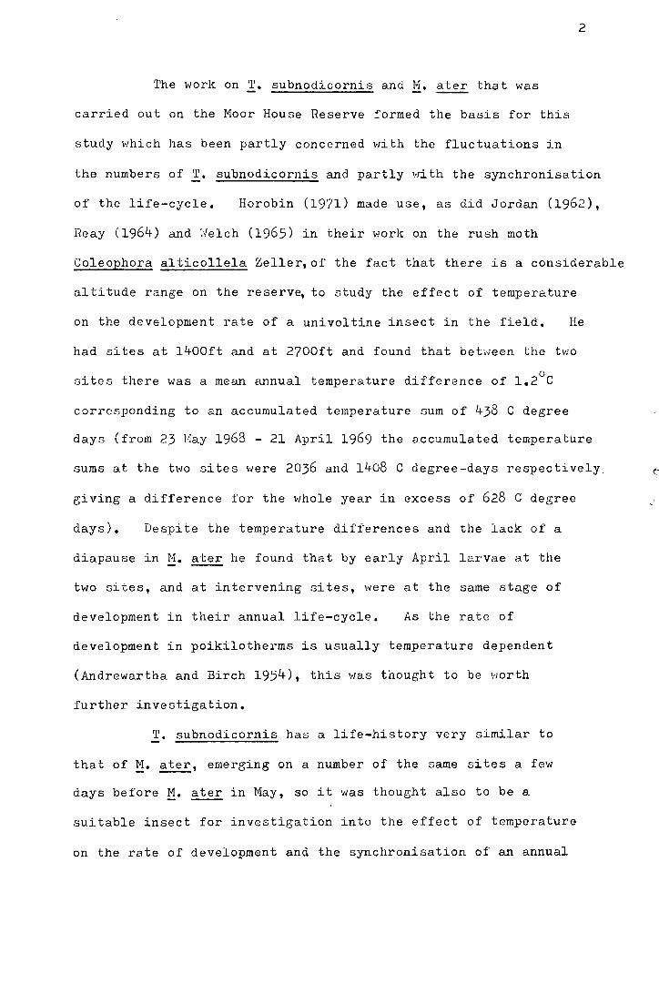
I. INTRODUCTION

This study has been concerned with the ecology of

moorland craneflies, particularly Tipula subnodicornis Zetterstedt,

and was carried out on the Moor House National Nature Reserve,

No. 80, an area of upland blanket-bog.

There is considerable literature on the taxonomy of

the Tipulidae in both hemispheres. In particular, Alexander (1920),

Dobrotw·orsky (1968, 197l•a, b,c), Ed.,.rards (1938, 1939), MannheimS(l940

onwards) and Coe (1950) have produced keys to the adults. Brindle

(1960 and 1967) and Chis1·rell (1956) describe fourth instar larvae

of most of the British Tipulidae.

Much of the work on craneflies has been concerned with

the few species of economic importance. Tipula paludosa ~1eigen

and 1· oleracea Linnaeus occur on farm land and their damage to

crops has been described by Rennie (1916, 1917), Loi (1965) and

Ricou (1968) among others. White (1951) studied 1· lateralis

Meigen in relation to the damage it caused in watercress beds.

The life-history and general biology of 1· paludosa was described

by Selke (19'~) and Maerks (1943), while Milne et al. (1965) and

Laughlin (1967) have related the abundance and growth rate of

the species to environmental conditions (rainfall and temperature

respectively).

Detailed studies on hro other species, 1· subnodicornis

and ~1olophilus ater Meigen, have been carried out by Coulson (1962),

Hadley (1969, 197la&b) and Horobin (1971) on the Moor House Reserve.

Community studies on craneflies have been carried out by Coulson

(1959), Crips and Lloyd (1954) and Freeman (1964, 1967, 1968) and

Freeman and Adams (1972), and the taxonomic works already referred

to give further ecological information.

1

The work on !• subnodicornis and ~· ater that was

carried out on the Moor House Reserve formed the basis for this

study which has been partly concerned with the fluctuations in

2

the numbers of 'I'. subnodicornis and partly v.ri th the synchronisation

of the life-cycle. Horobin (1971) made use, as did Jordan (1962),

Reay (1964) and ·:.felch (1965) in their \>JOrk on the rush moth

Coleophora alticollela Zeller,of the fact that there is a considerable

altitude range on the reserv~ to study the effect of temperature

on the development rate of a univoltine insect in the field. He

had sites at 1400ft and at 2700ft and found that bebieen the hio

sites there was a mean annual temperature difference of 1.2°C

corresponding to an accumulated temperature sum of 438 C degree

days (from 23 J·:Iay 1968 - 21 April 1969 the accumulated temperature

sums at the two sites were 2036 and 1408 C degree-days respectively ~

giving a difference for the whole year in excess of 628 C degree

days). Despite the temperature differences and the lack of a

diapause in M. ater he found that by early April larvae at the

two sites, and at intervening sites, were at the same stage of

development in their annual life-cycle. As the rate of

development in poikilotherms is usually temperature dependent

(Andrewartha and Birch 1954), this Has thought to be 1-10rth

further investigation.

T. subnodicornis has a life-history very similar to

that of~· ater, emerging on a number of the same sites a few

days before M. ater in May, so it was thought also to be a

suitable insect for investigation into the effect of temperature

on the rate of development and the synchronisation of an annual

life-cycle. The work in this study on the timing of emergence

in the field has been greatly facilitated by the presence of

soil temperature data provided by Horobin (1971) for different

altitude sites ru1d by the records from the Grant multichannel

recorder used during the International Biological Programme

for measuring the temperatures registered by thermistor probes

at different depths in blanket-bog. The daily readings from

the Moor House Meteorological Station have provided information

on year to year variation in temperature.

3

From 1953-1955 Coulson (1962) made a detailed population

study throughout the life-cycle of !• subnodicornis on an area

dominated by Juncus. In this study the same site has been

used and additional sites on Juncus and Eriophorum dominated

areas and blanket-bog have been started for comparative purposes.

Data have been accumulated on the numbers of fourth instar larvae

and adults present on these sites and the effect of density on

mortality has been investigated under experimental conditions.

Wing length, used extensively by Hemingsen (1956), Hemingsen

and Birger Jensen (1957, 1960, 1972) and Hemingsen and Nielsen

(1965) in other contexts, has been used to reflect the size of

adults on each site, so fecundity as well as mortality has been

estimated. The results from this study confirm the observations

of ~ulne et al. (1965) for !· paludosa and Coulson (1962) for

T. subnodicornis that drought in the early stages of development

causes a high mortality. Evidence for density dependent effects

on both mortality and fecundity has also been found and as this

is also the case for M. ater (Horobin 1971) the two species may

be compared.

Note

l. fhe specific names of plants mentioned in this thesis are

taken from Clapham et al. (1962) for flovtering plants, and

vJatson (1955) for mosses and liverworts.

2. 'rhe statistical analyses are based on Bailey (1959) and

Snedecor and Cochran (1967). \rlhen samples of less than

thirty are compared by means of a t-test the degrees of

freedom have been calculated by Bailey's method (page 51).

II. THE STUDY AREA

l. Description of the Moor House Reserve

The Moor House National Nature Reserve, \·Jestmorland

4

(N.H. 80 : Nat, Grid Ref. NY 758329) was described by Conway (1955).

It consists of 3850 hectares of which the greater part is blanket

bog lying on the eastern dip slope of the Pennine escarpment.

Knock Fell (2604ft, 794m), Great Dun Fell (2780ft, 845m) and

Little Dun Fell (2?6lft, 842m) which form part of the summit

ridge lie within the reserve while Cross Fell (2930ft, 893m),

the highest peak of the Pennines, is just to the north of the

reserve boundary. The River Tees forms the north and east

boundary of the reserve and also divides Cumberland and

Hestmorland along this stretch. The main tributary of the

Tees in its upper reaches is Trout Beck. The west scarp slope

overlooks the Eden Valley and the two main streams on this slope,

Crowdundle Beck and Knock Ore Gill,are tributaries of the

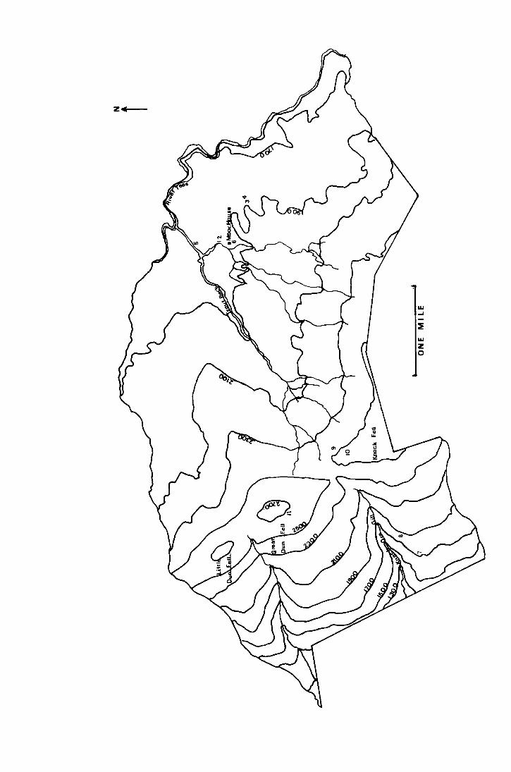
River Eden. Fig. 1 shows a map of the reserve showing relevant

landmarks a.nd the positions of the sites.

The geology of the reserve has been described by

Johnson and Dunham ( 196 3) • The underlying rock consists of

limestone and sandstone bands of the Carboniferous series.

Dun Fell is capped by sandstone and there are considerable

limestone outcrops on the west scarp. Limestone areas also

occur on the dip slope; Hoar House stands on one, but most of

the area is overlaid by peat, commonly about 1.5m deep, but

reaching a depth of 3m in places.

5

Peat occurs on all areas \·Jhere waterlogging takes place

and is a consequence of the low temperatures (mean annual

temperature for 1953-1965 was 5.1°C) and high rainfall (mean

annual rainfall for 1953-1965 vras 1869mm). This gives rise to

blanket bog with a characteristic flora. Sphagnum spp. are

constants and Calluna vulgaris and Er~horum vaginatum are dominant

over large areas, while !• angustifolium is abundant in the wetter

places, giving way to a total cover of Sphagnum on base poor flushed

areas. Where the peat is shallow or disturbed Juncus squarrosus

is often the dominant plant, possessing long roots which can reach

up to lm to the mineral soil.

The larger streams are bordered by beds of }Jea ty or

sandy alluvium and bare drift denoted by Johnson and Dunham (1963) as

"Mixed Bottom Lands". These and the limestone outcrops support

a varied flora in which Festuca ovina, Deschamusia caespitosa,

Agrostis tenuis, Holcus lanatus, Carex spp., Achillea millefolium

and 'l'hymus drucei are common.

Fig. l. Map of the Hoar House National Nature Reserve showing

the positions of the study areas.

l·1oor House site Dun l',ell sites

1. Nethorhearth ?. 1700ft

2. Above Netherhearth 8. 1900ft.

3. Bog End (Juncus) 9. 2500ft

4. Bog End (mixed moor) 10. 2550ft --------- ----

5. Trout Beck 11. 2700ft

6. Behind House

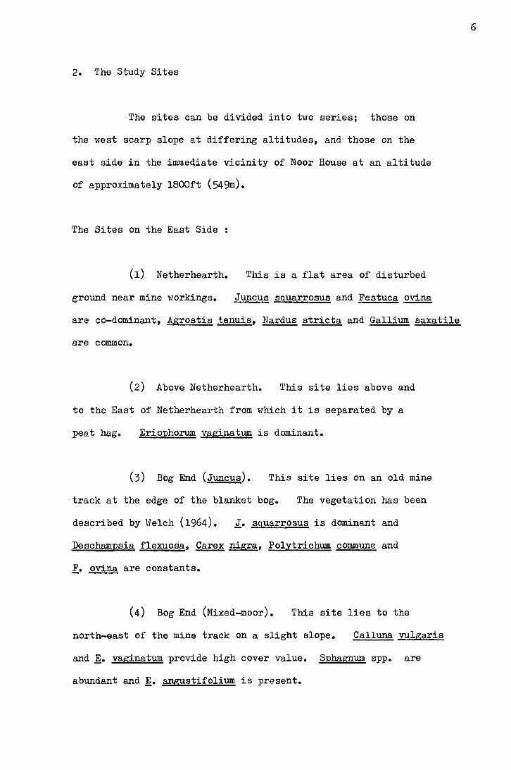
2. The Study Sites

The sites can be divided into t\'TO series; those on

the \'Test scarp slope at differing altitudes, and those on the

east side in the immediate vicinity of Moor House at an altitude

of approximately !800ft (549m).

The Sites on the East Side

(1) Netherhearth. This is a flat area of disturbed

ground near mine l'IOrkings. Juncus sguarrosus and Festuca ovina

are co-dominant, Agrostis tenuis, Nardus stricta and Gallium saxatile

are common.

(2) Above Netherhearth. This site lies above and

to the East of Netherhearth from rThich it is separated by a

peat hag. Eriophorum vaginatum is dominant.

(3) Bog End (Juncus). This site lies on an old mine

track at the edge of the blanket bog. The vegetation has been

described by Helch (1964). I· sguarrosus is dominant and

Deschampsia flexuosa, Carex nigra, Polytrichum commune and

l· ovina are constants.

(4) Bog End (Mixed-moor). This site lies to the

north-east of the mine track on a slight slope. Calluna vulgaris

and .§. vaginatum provide high cover value. Sphagnum spp. are

abundant and .§. angustifolium is present.

6

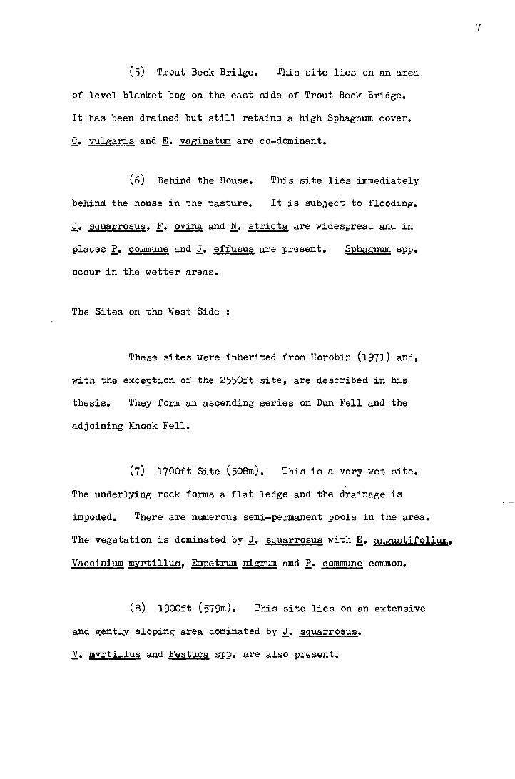
(5) Trout Beck Bridge. This site lies on an area

of level blanket bog on the east side of Trout Beck Bridge.

It has been drained but still retains a high Sphagnum cover.

Q. vulgaris and !· vaginatum are co-dominant.

(6) Behind the House.

behind the house in the pasture.

This site lies immediately

It is subject to flooding.

I· sguarrosus, l· ovina and li· stricta are widespread and in

places f. commune and l· effusus are present.

occur in the wetter areas.

The Sites on the v/est Side

Sphagnum spp.

These sites 'vere inherited from Horobin (1971) and,

l-Tith the exception of the 2550ft site, are described in his

thesis. They form an ascending series on Dun Fell and the

adjoining Knock Fell.

(7) 1700ft Site (508m). This is a very \-let site.

The underlying rock forms a flat ledge and the drainage is

impeded. There are numerous semi-permanent pools in the area.

The vegetation is dominated by l· sguarrosus with !• angustifolium,

Vaccinium myrtillus, Empetrum nigrum amd f. commune common.

(8) 1900ft (579m). This site lies on an extensive

and gently sloping area dominated by l· sguarrosus.

!· myrtillus and Festuca spp. are also present.

7

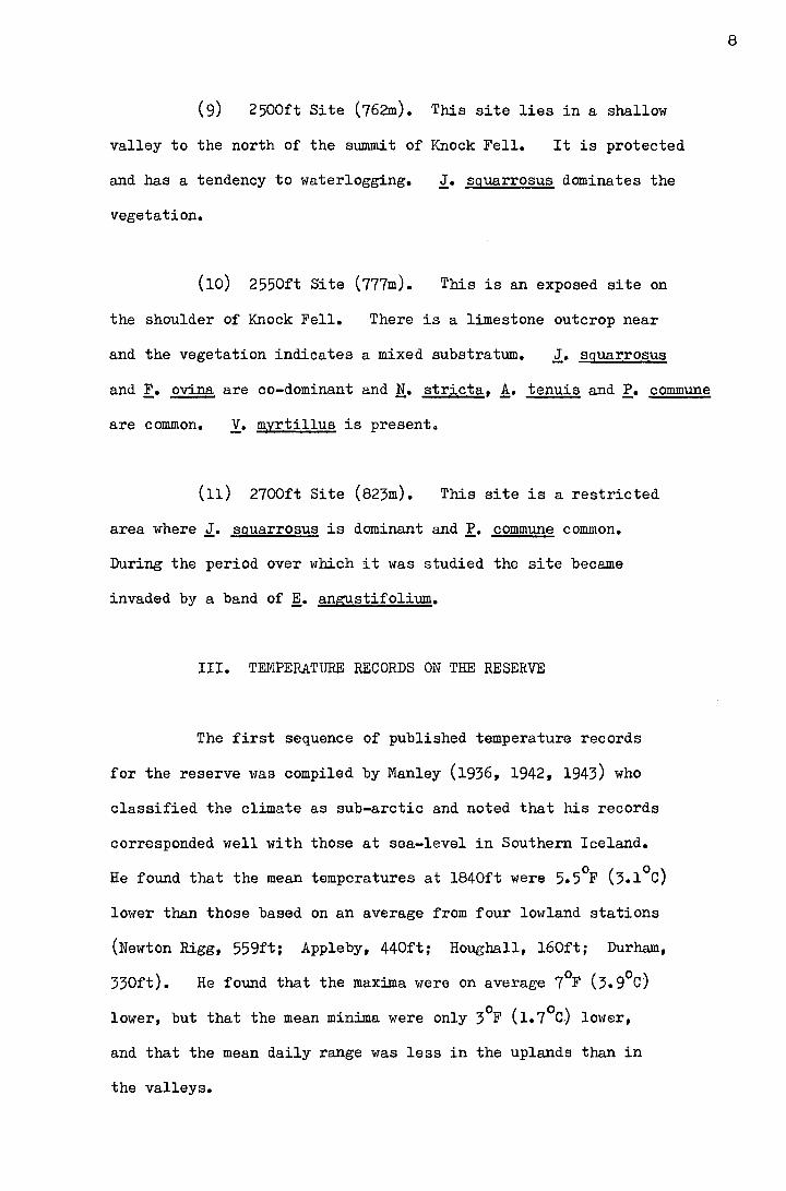
( 9) 2 500ft Site ( 762m). This site lies in a shallOli

valley to the north of the summit of Knock Fell. It is protected

and has a tendency to liaterlogging. I· sguarrosus dominates the

vegetation.

(10) 2550ft Site (777m). This is an exposed site on

the shoulder of Knock Fell. There is a limestone outcrop near

and the vegetation indicates a mixed substratum. I· sguarrosus

and !· ovina are co-dominant and !• stricta, !· tenuis and f. commune

are common. y. myrtillus is present.

(11) 2700ft Site (823m). This site is a restricted

area where I· sguarrosus is dominant and f. commune common.

During the period over rrhich it was studied the site became

invaded by a band of !· angustifolium.

III. TEMPERATURE RECORDS ON THE RESERVE

The first sequence of published temperature records

for the reserve "t'Tas compiled by Manley (1936, 1942, 1943) who

classified the climate as sub-arctic and noted that his records

corresponded rrell with those at sea-level in Southern Iceland.

He found that the mean temperatures at 1840ft were 5.5°F (3.1°C)

lo'l'rer than those based on an average from four lm1land stations

(Newton Rigg, 559ft; Appleby, 440ft; Houghall, 160ft; Durham,

330ft). He found that the maxima v1ere on average 7°F (3. 9°C)

1 b t th t th · · 1 3°F ( 1. 7°C.) lower, ower, u a e mean m1~a were on y _

and that the mean daily range l·ras less in the uplands than in

the valleys.

8

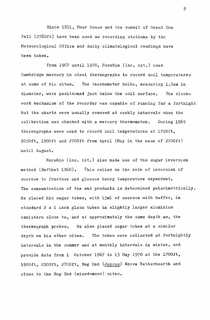
Since 1951, Jlioor House and the summit of Great Dun

Fell (2780ft) have been used as recording stations by the

Meteorological Office and daily climatological readings have

been ta.ken.

From 1967 until 1970, Horobin (lac. cit.) used

9

Cambridge mercury in steel thermographs to record soil temperatures

at some of his sites. The thermometer bulbs, measuring 1.5cm in

diameter, were positioned just below the soil surface. 'rhe clock-

work mechanism of the recorder was capable of running for a fortnight

but the charts were usually removed at weekly intervals when the

calibration was checked with a mercury thermometer. During 1969

thermographs were used to record soil temperatures at 1700ft,

2050ft, l900ft and 2700ft from April (May in the case of 2700ft)

until August.

Horobin (loc. cit.) also made use of the sugar inversion

method (Berthet 1960). This relies on the rate of inversion of

sucrose to fructose and glucose being temperature dependent.

The concentration of the end products is determined polarimetrically.

He placed his sugar tubes, with 15ml of sucrose with buffer, in

standard 2 x 1 inch glass tubes in slightly larger aluminium

canisters close to, and at approximately the same depth as, the

thermograph probes. He also placed sugar tubes at a similar

depth on his other sites. The tubes were collected at fortnightly

intervals in the summer and at monthly intervals in winter, and

provide data from 1 October 1967 to 13 May 1970 at the 1700ft,

1900ft, 2500ft, 2700ft, Bog End (Juncus) ~bove Netherhearth and

close to the Bog End (mixed-moor) sites.

As a control for the Berthet method, Horobin placed

sugar tubes by the thermometers in the meteorological screen.

10

He compared the mean temperatures derived from the meteorological

data and from the Cambridge recorders with the means calculated

from the sugar tubes in appropriate positions and obtained the

regression y = o.87x - 0.4 (where y is the true arithmetic mean

temperature in °C and x is that derived from the sucrose method)

with a correlation coefficient of r = +0.98, showing a close

linear relationship. There is therefore a useful and reliable

series of soil temperature data at sites of differing altitude

on the reserve.

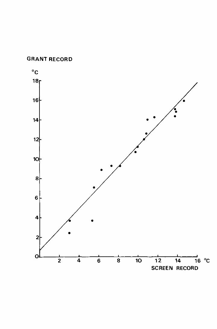
From the summer of 1968 until January 1972 a Grant

recorder was used by participants in the International Biological

Programme. This was set up on Syke Hill (1800ft, 550m) and

recorded the temperatures registered by probes at different

heights in the different types of vegetation and at various

depths below the vegetation. These data are now being analysed

in detail by Heal (pers. comm.) but I found that the data from

a probe at a depth of l.Ocm in Juncus squarrosus litter

correlated well with that from the meteorological screen when

the weekly means from April to September 1967 were compared.

The regression, Fig. 2, has the equation y = l.07x +- 0.71,

where y is the temperature in °C derived from the Grant weekly

means and x is that from the meteorological data. The correlation

coefficient, r = +0.98, provides justification for using the

Moor House data where soil temperatures would be more appropriate.

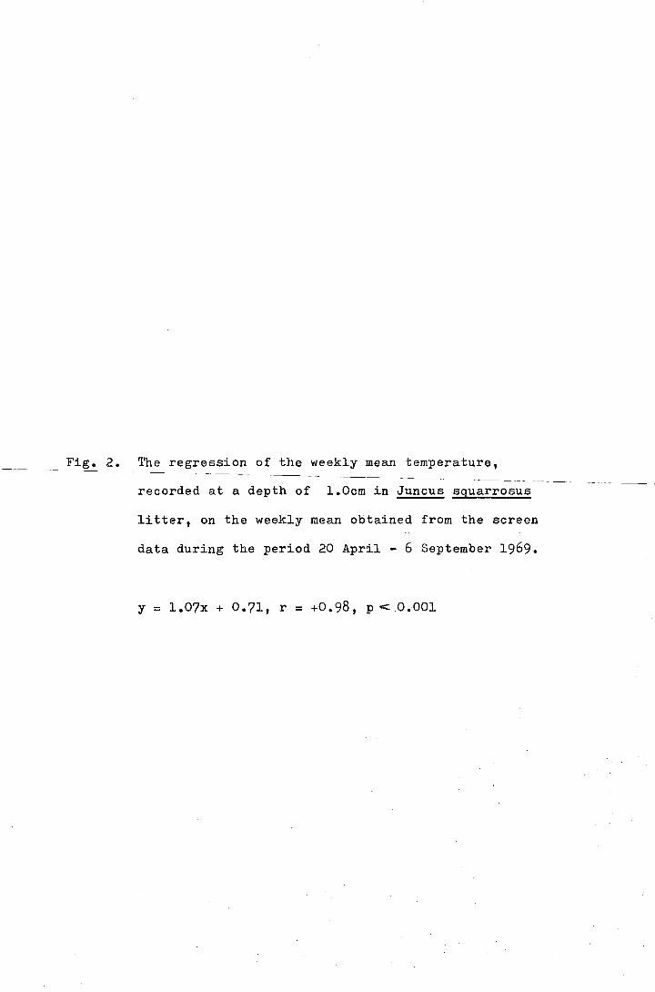
Fig. 2. The regression of the weekly mean temperature,

recorded at a depth of l.Ocm in Juncus sguarrosus

litter, on the weekly mean obtained from the screen

data during the period 20 April - 6 September 1969.

y = l.07x + 0.71, r = +0.98, p < 0.001

GRANT RECORD

o~----~--~~--~----~----~----~----~-----10 12 14 16 °C 2 4 6 8

SCREEN RECORD

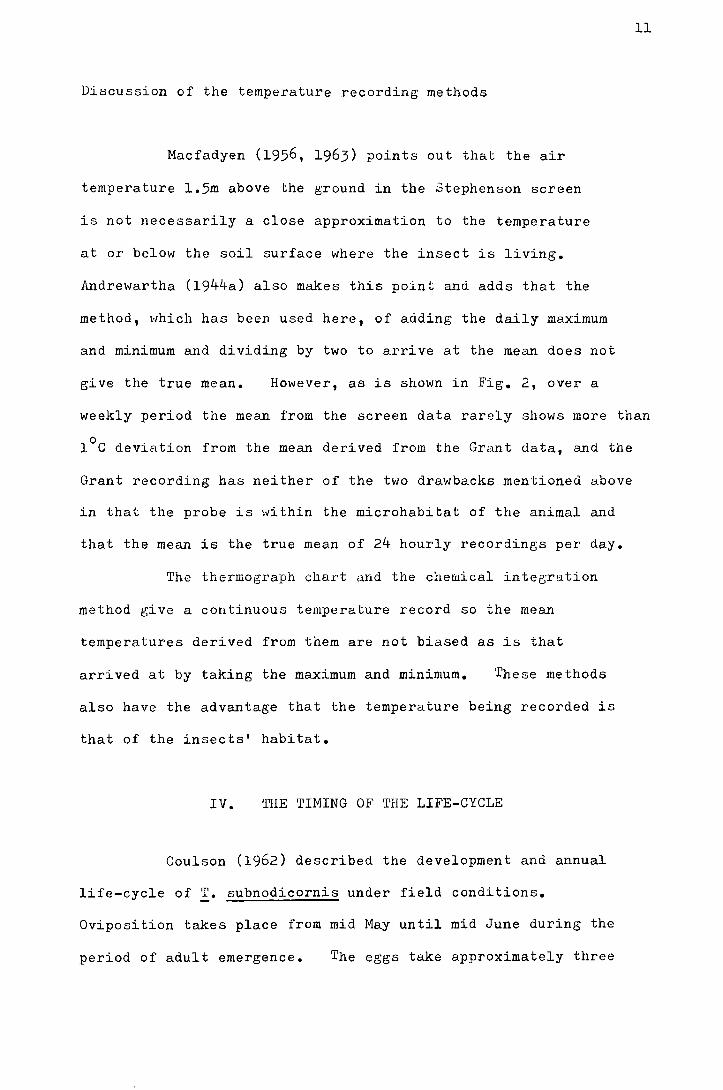
Discussion of the temperature recording methods

Macfadyen (1956, 1963) points out that the air

temperature 1.5m above the ground in the 3tephenson screen

is not necessarily a close approximation to the temperature

at or below the soil surface where the insect is living.

Andrewartha (1944a) also makes this point and adds that the

method, 1r1hich has been used here, of adding the daily maximum

and minimum and dividing by two to arrive at the mean does not

give the true mean. However, as is shown in Fig. 2, over a

11

weekly period the mean from the screen data rarely shows more than

l°C deviation from the mean derived from the Grant data, and the

Grant recording has neither of the two drawbacks mentioned above

in that the probe is vJithin the microhabitat of the animal and

that the mean is the true mean of 24 hourly recordings per day.

The thermograph chart and the chemical integration

method give a continuous temperature record so the mean

temperatures derived from them are not biased as is that

arrived at by taking the maximum and minimum. These methods

also have the advantage that the temperature being recorded is

that of the insects' habitat.

IV. 'l'HE 'l'IMING OF THE LIFE-CYCLE

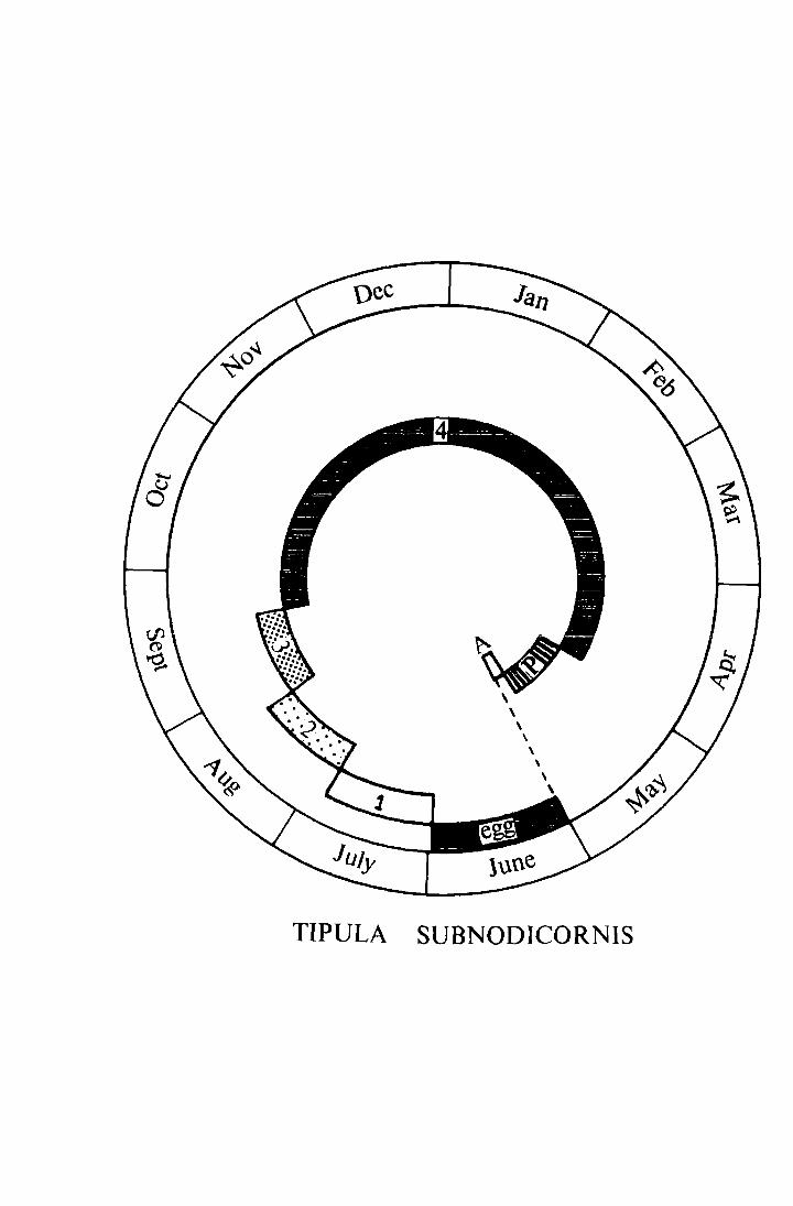
Coulson (1962) described the development and annual

life-cycle of !• subnodicornis under field conditions.

Oviposition takes place from mid May until mid June during the

period of adult emergence. The eggs take approximately three

12

weeks to hatch and give rise to first instar larvae. rewards

the end of July first instar gives place to the second which

lasts two to three weeks as does instar three. Most larvae

have entered instar four by the last week in September. All

larvae overwinter in instar four which is, like the other larval

instars, an active feeding stage. Pupation lasts three weeks

from about late April until mid May when the adults start emerging.

Fig. 3, trucen from Coulson (1962), gives a diagrammatic represent-

ation of the life-cycle in the field.

Coulson found that !• subnodicornis had a highly

synchronised emergence period from mid May until mid June.

At any one site the emergence took place over a three week

period with two thirds of the emergence occurring within eleven

days (S.D. = 5.5 days). Horobin (1971) found that both M. ater

and!· subnodicornis emerged later at higher altitudes. In 1970,

for instance, the mean date of emergence for T. subnodicornis at

2700ft was eight days behind that at 1700ft.

If development rate is linearly related to temperature

it is possible to calculate the temperature sum in degree-days

0 (calculated in this thesis as mean daily temperature above 0 C

multiplied by the number of days at that temperature) required

for development, as has been done for the codling-moth Enarmonia

pomonella L. (Glenn l922)and Acronycta rumicis L. (Danilevskii

The temperature sums at 1700ft and 2700ft on Dun Fell

for the period 9 June 1969 - 13 May 1970 were 2068 and 1717 °C

degree-days respectively. If the date of emergence were

dependent on the yearly temperature sum alone this difference

(17%) is too great to be compensJted by the eight day difference

Fig. 3. The life-cycle of !· subnodicornis at Moor House

(taken from Coulson 1962).

1 - 4 = larval instars

P = pupa

A = adult

\ \

' ' ' \ ' \

TIPULA SUBNODICORNIS

13

in the emergence means vthich, assuming a high mean daily

0 temperature of 10 C, could account for a maximum 80C degree-days.

" ' "

As T. subnodicornis lacks a diapause (Coulson 1962) there must

be some factor other than temperature sum accumulation that

influences the duration of the life-cycle. In order to

investigate this situation the relationship between temperature

and development rate at different stages of the life-cycle of

T. subnodicornis has been studied both in the field and in the

laboratory.

For convenience of study in the laboratory, the life-

history is considered in five stages : egg; larval 1; larval 2;

pupal; and adult. The first larval stage constitutes the period

of growth between hatching and attaining maximum weight, and the

second larval stage is that between achieving maximum \veight and

pupation. The field study has mainly centered on the timing

of emergence.

V. EMEHGENCE IN 'l'HE FIELD

Horobin (1971) found that when sods containing M. ater

were transferred from one site to another, even as close to the

emergence period as 15 days before the mean emergence date on

the host site, the means for the transferred groups approximated

much more closely to the mean on the host site than to those of

the sites where they originated. For example, the mean date

of emergence from sods transferred from 2700ft to 1400ft on

13 Nay 1970 was 29 May (s.e. ! 0.2). The mean date of emergence

+ at 2700ft was 14 June (s.e. - 0.2) and of controls on the host

14

+ site 28 May (s.e. - 0.1). He found no correlation between the

yearly temperature sum El.t each site and mean emergence date at

that site, but suggested that larval development had finished

by early spring and that pupation was initiated by the passing

of a temperature threshold. This would occur earlier on lower

and more sheltered sites and would explain the sequence on Dun

Fell. As T. subnodicornis has a life-cycle similar to M. ater

and emerges a few days before ~· ater in the same sequence on

Dun Fell it was thought interesting to compare the two.

1. Sampling method

The most accurate method to monitor the emergence

pattern is to use emergence traps (Hadley 1969, Horobin 1971).

However, in the present study the low densities of T. subnodicornis

and the number of sites used made this impractical and an alternative

method was sought.

Hadley (1969) and Horobin (1971) both used pitfalls to

record the emergence of~ ater on a number of sites and Coulson

(1962) used sticky traps for !• subnodicornis. Pitfall traps

are not reliable indicators of population density (Mitchell 1963,

Greenslade 1964) due to the catch being dependent in part on the

activity of the insect as v;ell as on the numbers present, and

the same criticism applies to sticky traps. However, Hadley (1969)

found that for the wingless and short-lived ~· ater pitfall traps

gave a valid representation of the emergence pattern. He compared

direct population estimates, arrived at by suction trapping within

2 0.05m emergence traps, and indirect estimates obtained from both

sticky traps and pitfalls on the same sites. He found that,

using eight pitfalls and eight sticky traps, the first and

last days of the emergence, the range and the mean date were

not significantly different from those obtained by the direct

method.

As T. subnodicornis also has a short adult life and

only the males are able to fly, it was thought probable that

either sticky traps or pitfalls could be used to reflect the

pattern of emergence in this study. In the first instance

pitfall catch and sticky trap catches were compared, and in a

later year a comparison between emergence from enclosures and

the pitfall catch was made.

During thio study each Moor House site had 20 1 lb

jam jars placed (except at the Bog End (Juncus) site 1-.rhere

there were two lines) in a grid of four lines of five. On

the Dun Fell sites there were 10 jars in two rows of five at

each site. Each jar was separated from its neighbour by

approximately 2m and sunk with its rim flush with the soil

surface and filled to a depth of about 2 em with a weak

detergent solution. ~he detergent acted as a wetting agent

preventing the escape of insects once they had made contact

with the water film. The traps were emptied daily on the

Noor House site in 1970 and 1971 and on alternate days in

1972. On the Dun Fell they were emptied daily in 1971 and

1972 and on alternate days in 1970.

la. Comparison between sticky trap and pitfall catches

In 1970 four sticky traps similar to those described

by Broadbent (1948) were erected at the four corners of the

15

Netherhearth site. Each trap consisted of an aluminium cylinder

30cm in length and 13.7cm diameter. The cylinders were covered

with polythene, held in place by clothes pegs, and covered with

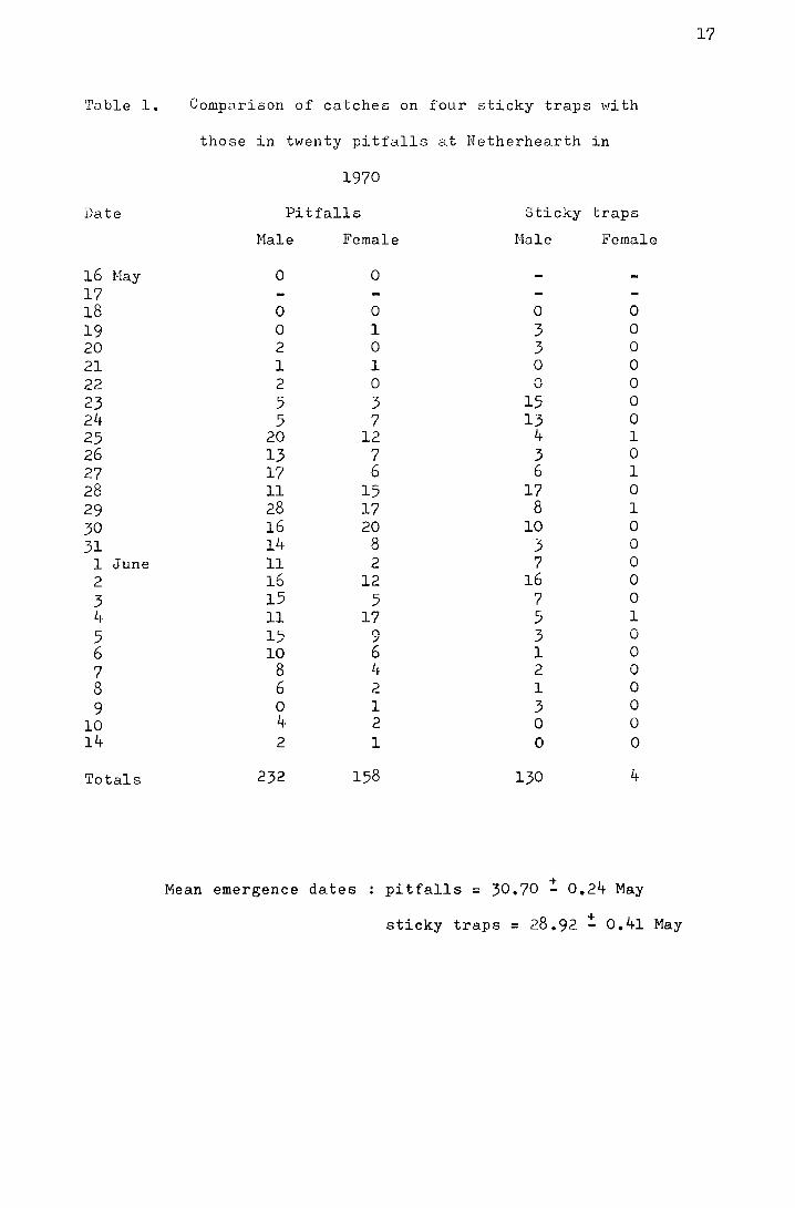
"Stick-tite", a tree banding preparation. In Table 1 the daily

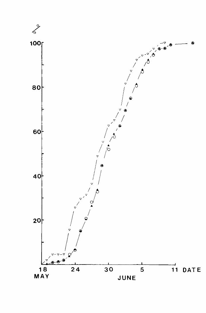
catches on both types of trap are compared. In Figure 4 the

cumulative percentages of flies trapped are plotted for both

pitfall and sticky traps. The mean date for pitfall catches,

30.70! 0.24 Nay, is significantly different from that for the

I + sticky traps, 28.92-0.41 Nay (t = 3.16, p<0.002), but the

first -days are the same and although the last days are not,

the patterns are very similar.

A possible explanation for the differences in the

mean dates obtained by the two trapping methods might be provided

by the fact that the sticky traps catch very few females. If

males emerged earlier in the emergence period than females, as

is the case with £1. ater (Hadley 1969), the mean emergence date

registered by the pitfall catch (in which both sexes are

represented) would be later than that for the sticky trap catch

lvhere males almost exclusively are caught. It can be seen from

Figure 4 that the male cumulative percentage pitfall catch follm'ls

the combined catch very closely and has an identical mean,

indicating that the percentage of the total male catch on the ground

is similar to that of the females at any period in time. This,

however, does not invalidate the suggestion that males might be

emerging earlier than females if a behavioural difference is

involved.

16

•ra.ble 1.

Date

16 Hay 17 18 19 20 21 22 23 24 25 26 27 28 29 30 31

1 June 2 3 li

5 6 7 8 9

10 14

Totals

Comparison of catches on four sticky traps with

those in twenty pitfalls at Netherhearth in

1970

Pitfalls Sticky traps

Hale Female Nale Female

0 0

0 0 0 l 2 0 l l 2 0 5 3 5 7

20 12 13 7 17 6 ll 15 28 17 16 20 14 8 11 2 16 12 15 5 11 17 15 9 10 6

8 l~

6 2 0 1 4 2 2 1

232 158

Mean emergence dates

0 0 3 0 3 0 0 0 0 0

15 0 13 0

4 l 3 0 6 l

17 0 8 l

10 0 3 0 7 0

16 0 7 0 5 1

3 0 1 0 2 0 l 0 3 0 0 0 0 0

130 4

pitfalls = 30.70 ~ 0.24 May

sticky traps = 28.92 ~ 0.41 May

17

Fig. 4. The accumulated percentage pitfall and sticky trap

catches of T. subnoiflcornis at--Netherliearth in 1"970

plotted against date.

-v sticky trap ( N = 134)

a pitfall, both sexes (N = 390)

0 pitfall, male (N = 232)

,? 0

100

80

60

40

20

18 MAY

24 30 5 11 OAT E JUNE

18

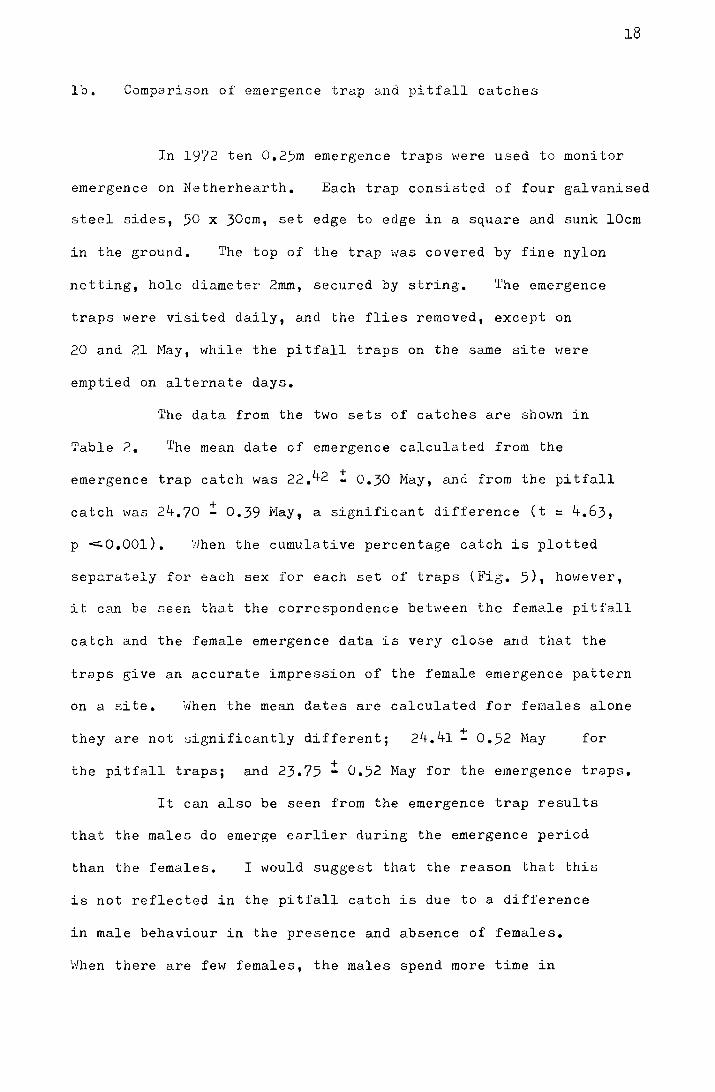
lb. Comparison of emergence trap and pitfall catches

In 1972 ten 0.25m emergence traps were used to monitor

emergence on Netherhearth. Each trap consisted of four galvanised

steel sides, 50 x 30cm, set edge to edge in a square and sunk lOcm

in the ground. The top of the trap was covered by fine nylon

netting, hole diameter 2mm, secured by string. 'I.'he emergence

traps were visited daily, and the flies removed, except on

20 and 21 Hay, while the pitfall traps on the same site 1·1ere

emptied on alternate days.

The data from the two sets of catches are shown in

Table 2. The mean date of emergence calculated from the

emergence trap catch was 22.42 ! 0.30 May, and from the pitfall

catch was 24.70 ! 0.39 May, a significant difference (t = 4.63,

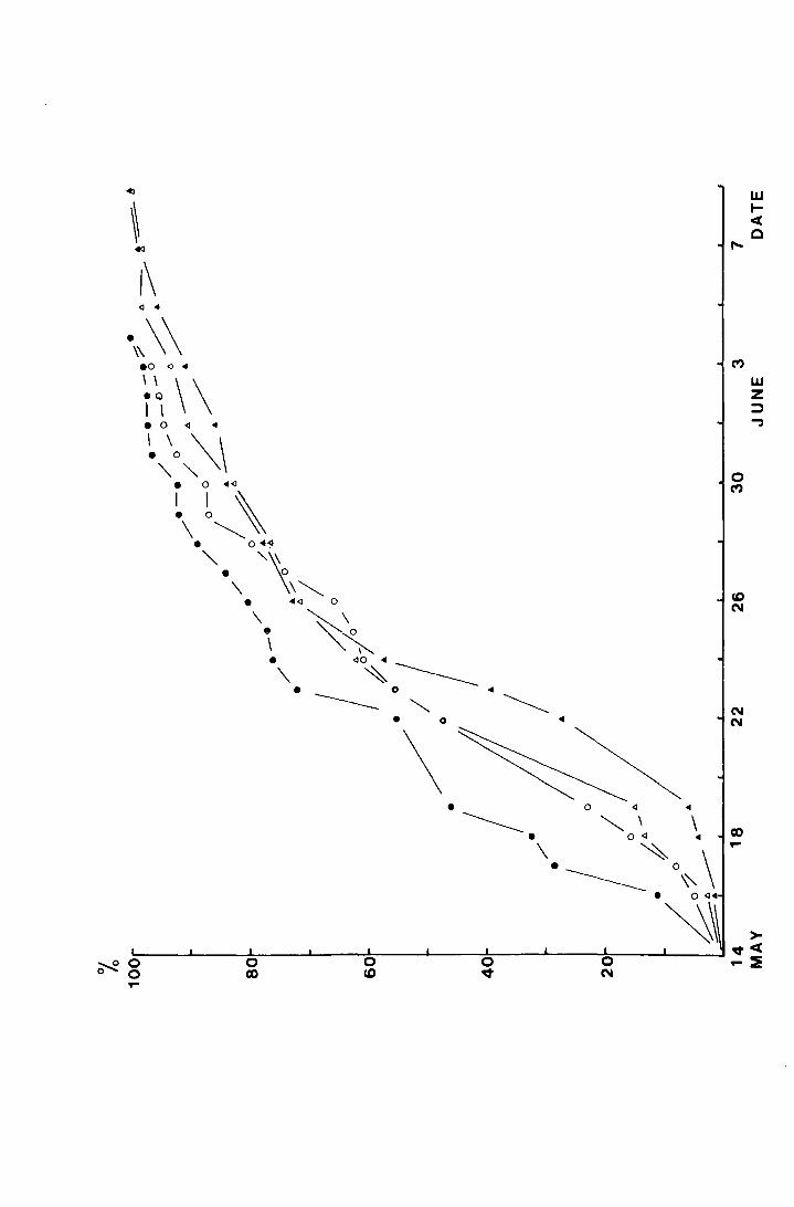
p c::::.O.OOl). 'crihen the cumulative percentage catch is plotted

separately for each sex for each set of traps (Fig. 5), however,

it can be seen that the correspondence between the female pitfall

catch and the female emergence data is very close and that the

traps give an accurate impression of the female emergence pattern

on a site. When the mean dates are calculated for females alone

they are not significantly different; 24.41! 0.52 May for

the pitfall traps; and 23.75 ! 0.52 May for the emergence traps.

It can also be seen from the emergence trap results

that the males do emerge earlier during the emergence period

than the females. I would suggest that the reason that this

is not reflected in the pitfall catch is due to a difference

in male behaviour in the presence and absence of females.

When there are few females, the males spend more time in

searching flight just above the vegetation than they do on the

ground. It is only when there are large numbers of females

present that substantial numbers of males descend to the

vegetation and are at risk of falling into the pitfalls.

This hypothesis explains why the male component of the pitfall

catch follows the female catch so closely and why the male

sticky trap catch gives an earlier mean emergence date than

the pitfall catch.

The longer continuation of the pitfall catch

present in both sexes can be accounted for by the life-spans

of the adult. Coulson (1956) calculated from mark recapture

experiments that the life expectation for the male was between

48 and 22hrs from the hour of ce..pture, and that for the female

between 32 and 15hrs.

On the basis of the comparisons made between pitfall

and emergence trap catches it vias decided that, as for N. ater,

the pitfall catch gave an accurate representation of the

emergence pattern for female T. subnodicornis. For the

purposes of year to year and site to site comparison it was

not thought necessary to make any adjustment to the calculated

mean emergence date to allow for the earlier appearance of the

males, but if an absolute date for the mean emergence for both

sexes were required, the emergence trap data would indicate

that this is two days before that calculated from the pitfall

data.

19

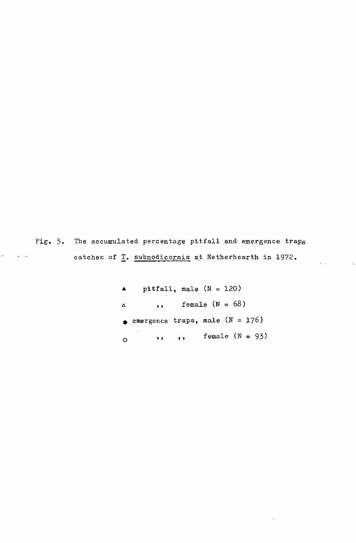
Fig. 5. The accumulated percentage pitfall and emergence traps

catches of T. subnodicoriJiS at Netherhearth in 1972.

• pitfall, male (N = 120)

/::,. ' ' female (N = 68)

• emergence traps, male (N = 176)

0 ' ' ' ' female (N = 93)

~0 0 0

0 CX)

0 <D

,...

0 (I)

N N

w t­<(

c

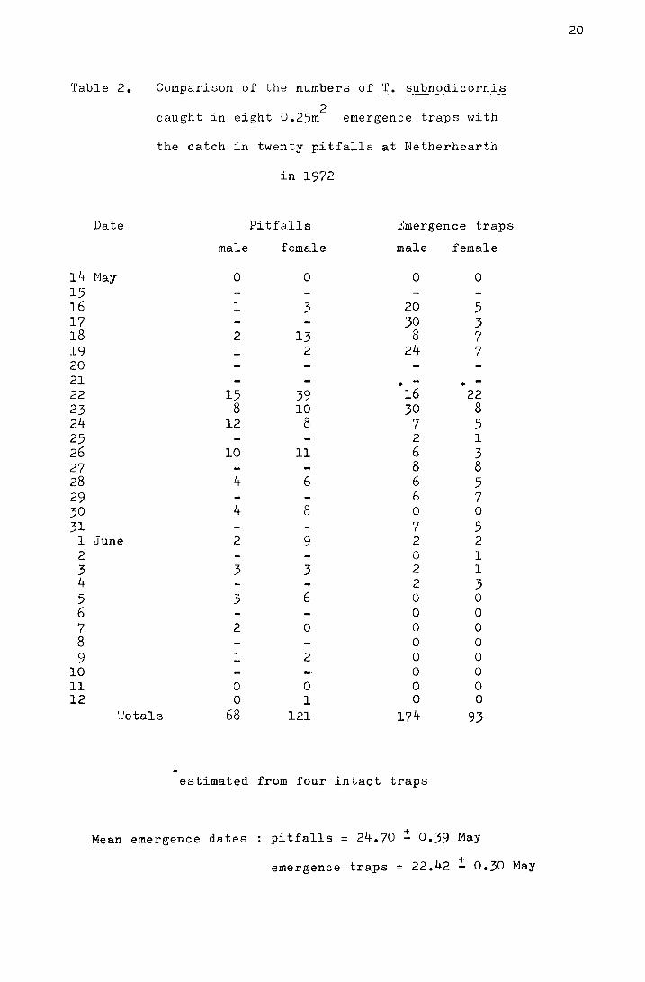
Table 2. Comparison of the numbers of ~· subnodicornis

caught in eight 0.25m2

emergence traps with

14 15 16 17 18 19 20 21 22 23 24 25 26 27 28 29 30 31

1 2 3 4 5 6 7 8 9

10 ll 12

the catch in twenty pitfalls at Netherhearth

in 1972

Date Pitfalls Emergence traps

male female male female

Nay 0 0 0 0

l 3 20 5 30 3

2 13 8 7 l 2 24 7

. - • 15 39 16 22

8 10 30 8 12 8 7 5

2 1 10 11 6 3

8 8 4 6 6 5

6 7 4 8 0 0

7 5 June 2 9 2 2

0 l 3 3 2 1

2 3 3 6 0 0

0 0 2 0 0 0

0 0 l 2 0 0

0 0 0 0 0 0 0 1 0 0

Totals 68 121 174 93

• estimated from four intact traps

Mean emergence dates pitfalls = 24.70 ~ 0.39 May

+ emergence traps = 22.42 - 0.30 May

20

2. Results from the pitfall data

The emergence data for the four Moor House sites

from 1969-1972 and for the Dun Fell sites from 1970-1972 are

shown in Tables I-IV in the appendix. Figs. I-III, also in

the appendix, show the accumulated percentage daily catch

plotted against the date for each site for 1970-1972 (the

catches on Dun Fell in 1972 have been omitted due to the

small sample size). In Table 3 the me<:m and median dates

of emergence on the four Moor House sites for 1969-1972 are

shown.

It can be seen from Table 3 and Figs. I-III that

the emergence pattern takes the form of an approximately

~

symetrical distribution where the mean is equal to the median. ~

The deviation from the normal distribution is discussed in the

21

next section, but, as it was in most cases small, the differences

in mean emergence dates have been tested, using Student's t-test.

From Table 4 it can be seen that mean emergence dates differ

significantly on the same site from year to year, and on

different sites,(with the exception of Netherhearth and

Bog End (mixed-moor) in 1971 ang 1972) within the same year.

As Horobin (1971) found no correlation between the

mean emergence date of ~· ater and the temperature sum

accumulated during the life-cycle at each site and suggested

that pupation was triggered by the passing of a temperature

threshold in spring, it was decided to look at the relationship

between the timing of the emergence period of !• subnodicornis

and spring temperature. The effect of temperature during the

emergence period has been considered separately from that of

the earlier spring temperature.

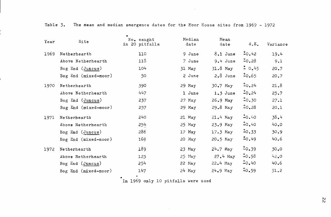
Table 3. The mean and median emergence dates for the Moor House sites from 1969 - 1972

• Year Site No. caught Median Mean

in 20 pitfalls date date S.E. Variance

1969 Netherhearth 110 9 June 8.1 June !o.42 19.4 Above Netherhearth 118 7 June 9.4 June !o.28 9.1

Bog End (Juncus) 104 31 May 31.8 May ! 0!45 20.7 Bog End (mixed-moor) 50 2 June 2.8 June :!:o.6s 20.7

1970 Netherhearth 390 29 May 30.7 Nay !o.24 21.8

Above Netherhearth 447 l June 1.3 June + -0.24 25.7 Bog End (Juncus) 237 27 May 26.9 May !o.3o 27.1

Bog End (mixed-moor) 257 29 May 29.8 May !o.28 20.1

1971 Netherhearth 240 21 May 21.4 May :!:o.4o 38.4

Above Netherhearth 25~~ 25 May 23.9 May :!:o.4o 4o.o

Bog End (Juncus) 286 17 May 17.3 May !0.33 30.9

Bog End (mixed-moor) 169 20 May 20.5 May !o.49 40.6

1972 Netherhearth 189 23 May 24.7 May + -0.39 30.0

Above Netherhearth 125 25 Hay 27.4 Nay :!:o.s8 42.0 Bog End (Juncus) 254 22 May 22.4 May :!:o.4o 40.6

Bog End (mixed-moor) 147 24 :tviay 24.9 Hay + -0.59 51.2

"' In 1969 only 10 pitfalls were used

1\) 1\)

2a. The effect of tempera~ure during the emergence period

The Nethcrhearth si~e has been chosen to compare the

variation in emergence pattern fro~ year to year because it

provides a relatively complete set of data and it is near the

meteorolocical screen whence the daily temperature data have

been obtained. The percentage accumulated pitfall catch for

each day has :i:'irst been plotted against date ar1cl tnen against

accumulated temperature in C degree-days, which have been

calculated from the screen daily ~eans (max + tlin/2), on nor;nal

probability paper (Figs. 6 - 9). It can be seen that plotting

23

against accumulated temperature rather than date has a normalising

effect. '.2i~e 1972 e::1ergence trap dctta havl!. also been treated in

the sc..me i·1ay, ~"ic. 10, und it can be scen 'chat the temperature

effect is not just the result of increased activity on hbtter

days, but is also caused ~y more adults emerging.

Although the temperature during the emergence period

~edifies the normal distribution, the effect that this has in

mo::;t years is .small, and in no ca.se .:.:.oes tll.e date on i·lhich the

mean i:~ ac curDula ted C deL-ree-d.o.ys falls differ significa."l tly from

the arithmetic mean.date. This is shown in Table 5. The comparison

between emergence periods based on mean dates is therefore felt to be

legi timate.o

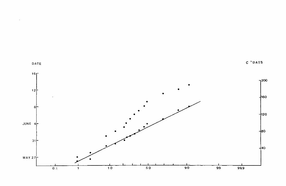
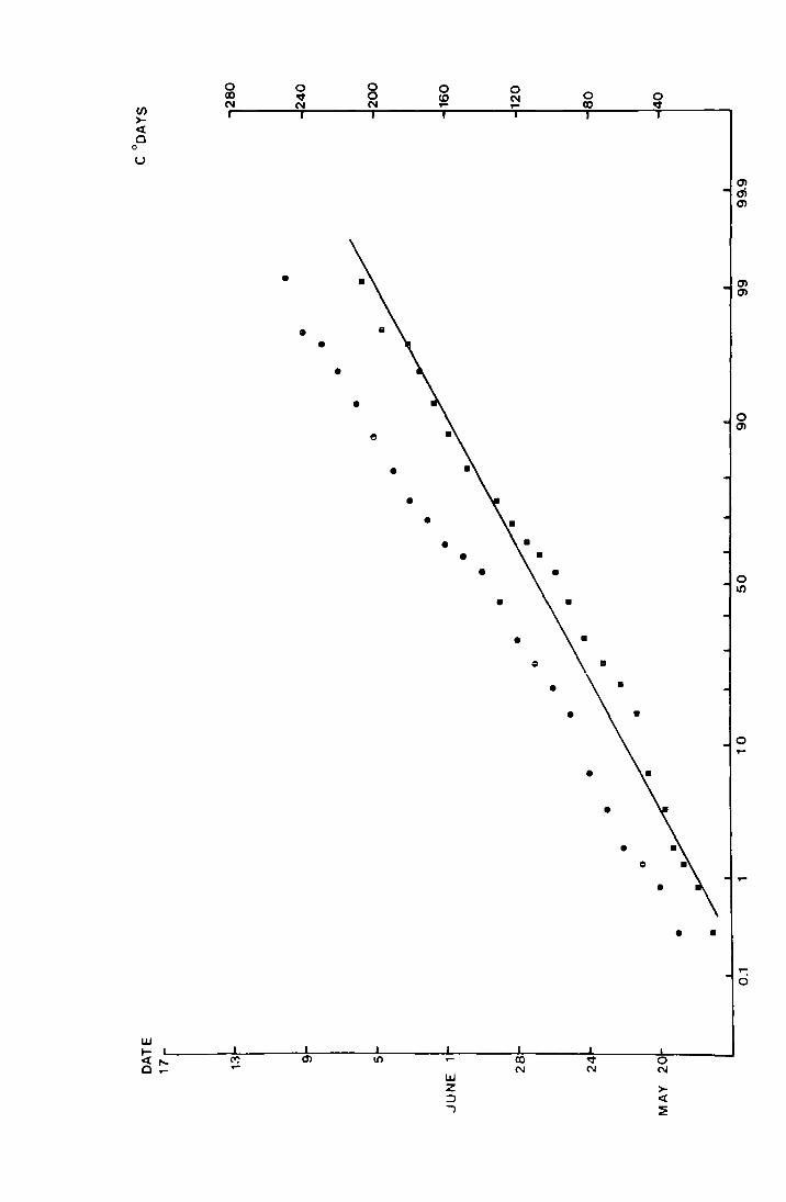
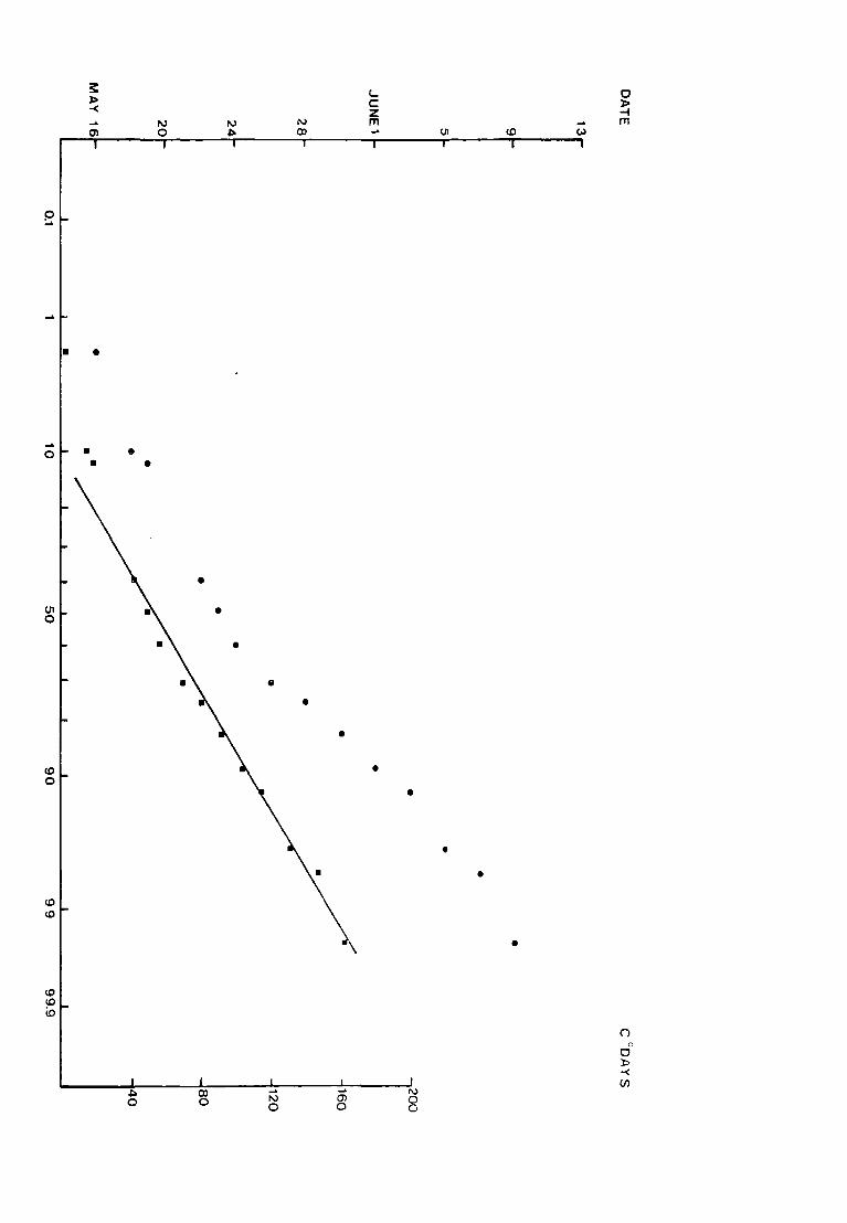
Fig. 6. The accumulated percentage pitfall catch at Netherhearth

·in-:t-~69 plo-tted against date_ an_d_against __ accumul_ated

C degree-days on normal probability paper.

• date

• C degree-days from the day before the

first fly was caught

(N = 110 )

DATE c 0 DAYS

200

• •

• 160

120

80

40

0.1 1 0 so 90 99 99.9

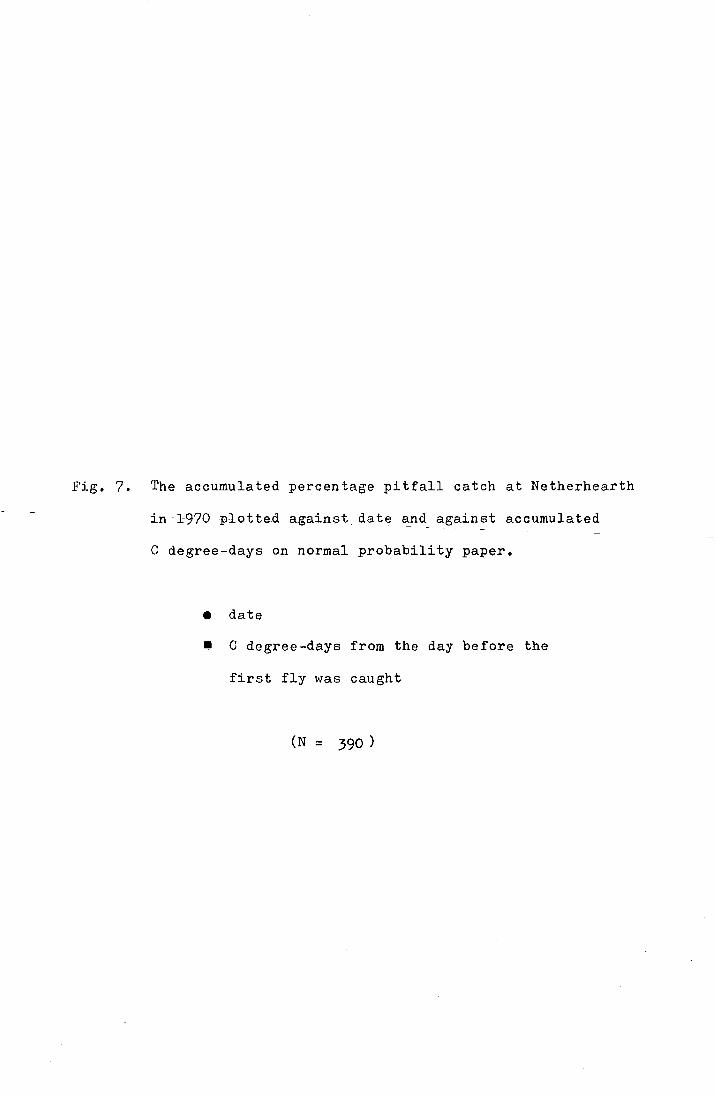
Fig. 7. The accumulated percentage pitfall catch at Netherhearth

in -l-97G plotted again9t date ~nd_ a_gain~t accumulated

C degree-days on normal probability paper.

• date

• C degree-days from the day before the

first fly was caught

(N = 390 )

u

•

• • •

0 N ~

• •

=

0 m

0 ~

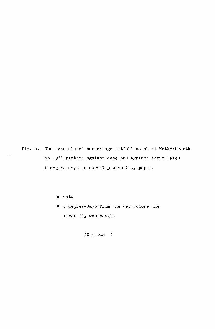
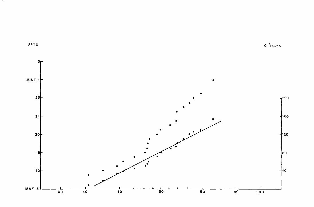
Fig. 8. The accumulated percentage pitfall catch at Netherhearth

in 1971 plotted again-st date and against accumulated

C degree-days on normal probability paper.

• date

• C degree-days from the day before the

first fly was caught

(N = 240 )

DATE c 0

0A y s

JUNE 1 •

G

• 200

• •

• 160

•

120

80

40

0.1 MAY 8 90 99 1.0 50 10 99.9

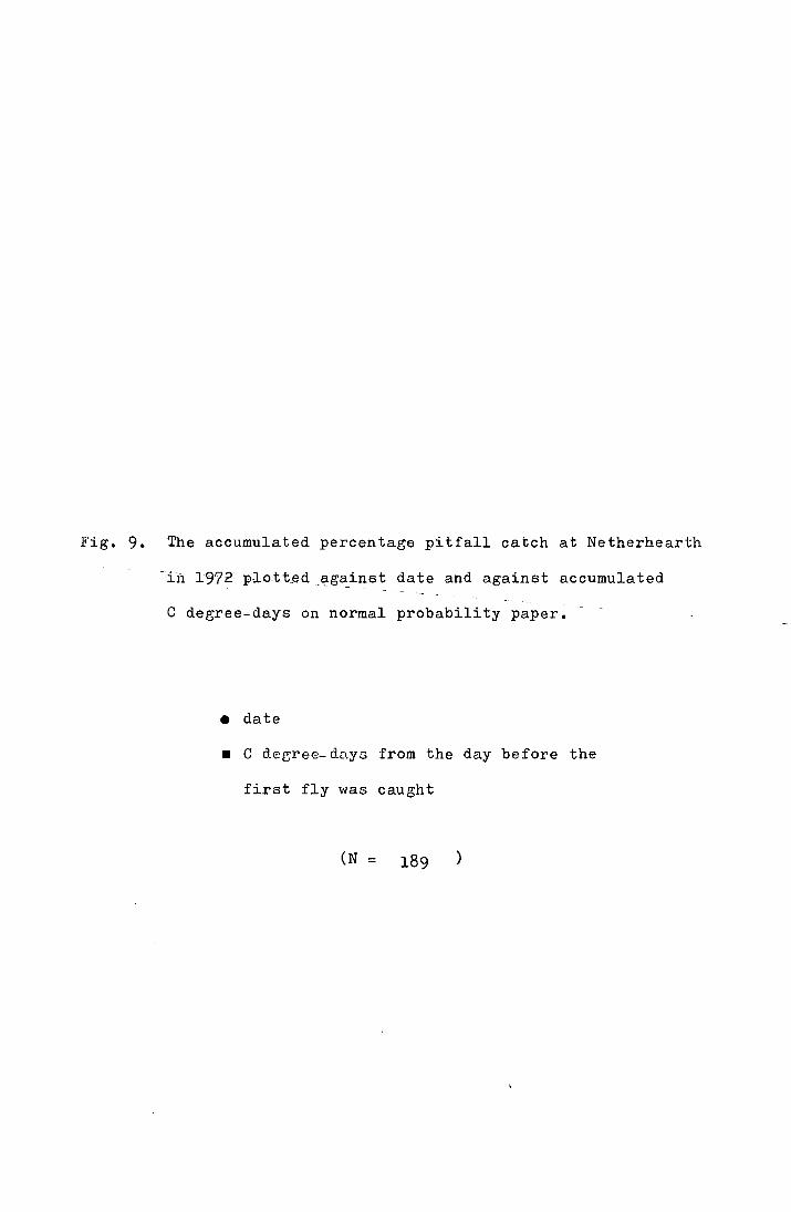
Fig. 9. The accumulated percentage pitfall catch at Netherhearth

-in 19?2- plo-tt_ed_~g~inst date and against accumulated

C degree-days on normal probability paper~

• date

• C detjree- days from the day before the

first fly was caught

(N = 189 )

p ....

.... 0

U1 0

CD 0

s:: l> -<

• •

.... N 0

N OJ

.... (]) 0

L c z m

• •

•

N 0 0

•

•

0 l> -t m

() 0

0 X:. -< (f)

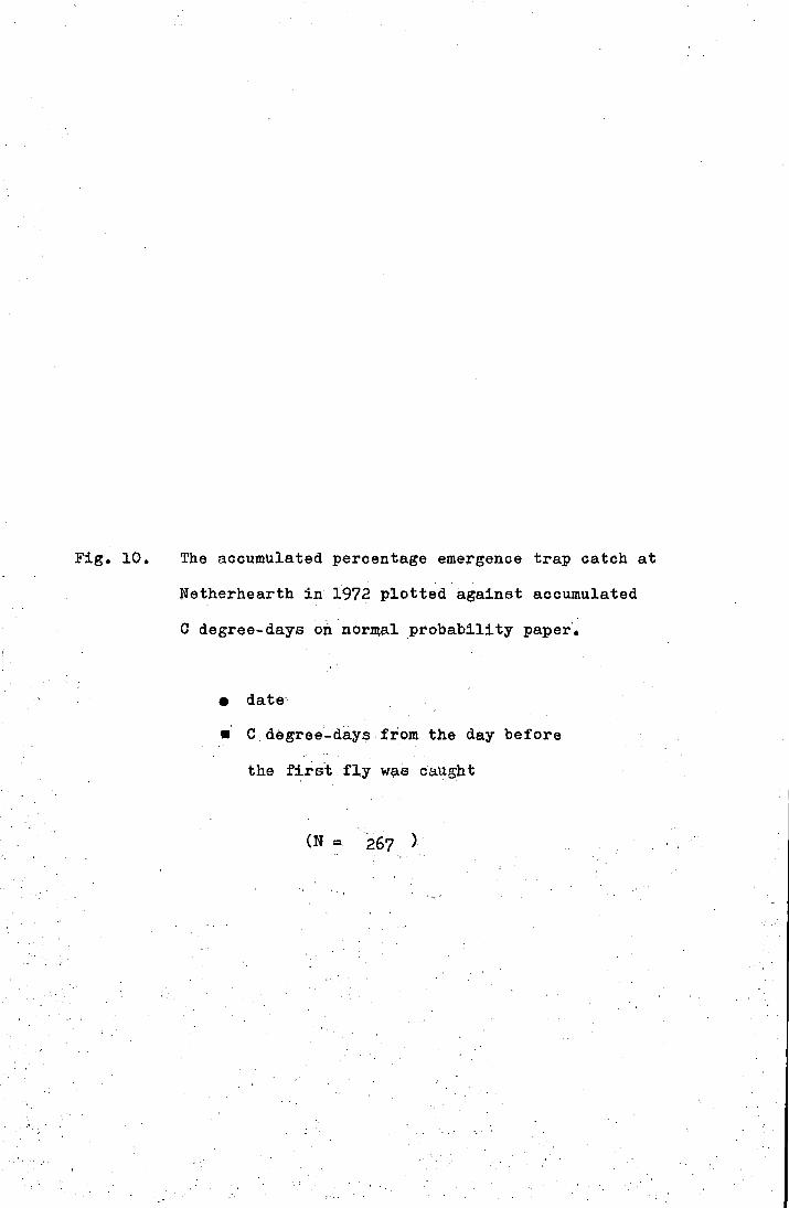
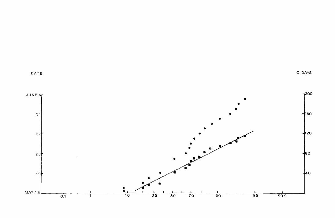
Fig. 10.

'·'

The accumulated percentage emergence trap catch at

Netherhearth in 197~ plotted against accumulated

C degree- days on normf3.1 probability pap err.

e datec

• C degree-days from the day before

the first fly w~;~.s caugb t

(N = 267 )

DATE C 0 DAYS

JUNE 4--

• •

• 3"1•·· •

• •

• 27 20

23 80

19 40

MAY 15 -0.1 1 50 99

24

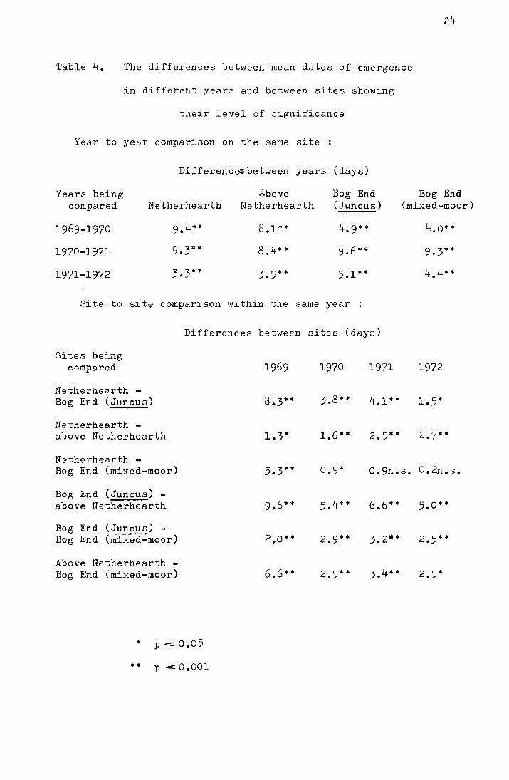
'l'able 4. The differences beh1een mean dates of emergence

in different years and between sites showing

their level of significance

Year to year comparison on the same site

Differencesbetween years (days)

Years being Above Bog End Bog End compared Netherhearth Netherhearth (Juncus) (mixed-moor)

1969-1970 9.4** 8.1 ** 4.9** 4.o**

1970-1971 9. 3""'' 8.4*"' 9.6""" 9.3*"'

1971-1972 3~3"'* 3-5** 5.1"'"' 4.4*"'

Site to site comparison within the same year :

Differences between sites (days)

Sites being compared 1969 1970 1971 1972

Netherhearth -Bog End (Juncus) 8.3** 3.8."' 4.1"'"' 1.5*

Netherhearth -above Netherhearth 1.3* 1.6·· 2.5** 2.7**

Netherhearth -Bog End (mixed-moor) 5.Y'* 0.9* 0.9n.s. o.an.s.

Bog End (Juncus) -above Netherhearth 9.6** 5.4** 6.6*"' 5.0**

Bog End (Juncus) -Bog End (mixed-moor) 2.o•• 2.9** 3.2** 2.5**

Above Netherhearth -Bog End (mixed-moor) 6.6•• 2.5** 3.4** 2.5"'

* p ~ o.o5

•• p <::: 0.001

25

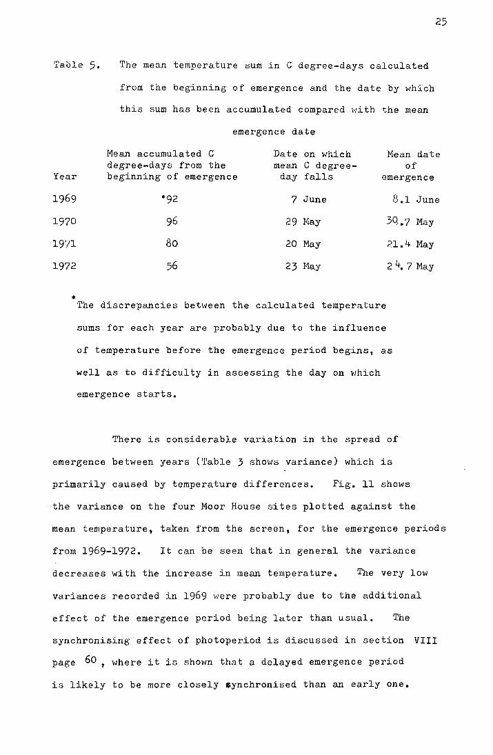
Table 5. The mean temperature sum in C degree-days calculated

from the beginning of emergence and the date by which

this sum has been accumulated compared vii th the mean

emergence date

Mean accumulated C Date on which Mean date degree-days from the mean C degree- of

Year beginning of emergence day falls emergence

*92 7 June 8.1 June

1970 96 29 May 3q.7 May

19?1 80 20 May 21.4 May

1972 56 23 Nay 2 4. 7 May

* The discrepancies between the calculated temperature

sums for each year are probably due to the influence

of temperature before the emergence period begins, as

well as to difficulty in assessing the day on which

emergence starts.

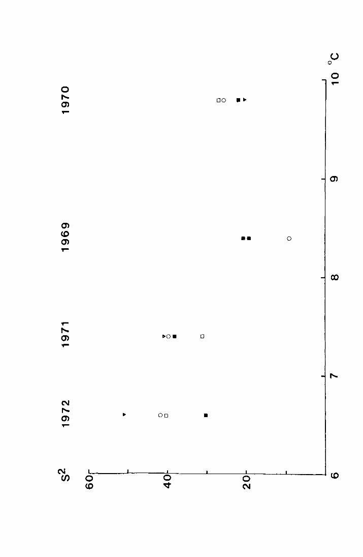
There is considerable variation in the spread of

emergence between years ('fable 3 shows variance) which is

primarily caused by temperature differences. Fig. 11 shows

the variance on the four Moor House sites plotted against the

mean temperature, taken from the screen, for the emergence periods

from 1969-1972. It can be seen that in general the variance

decreases with the increase in mean temperature. The very low

variances recorded in 1969 were probably due to the additional

effect of the emergence period being later than usual. The

synchronising effect of photoperiod is discussed in section VIII

page 60 , where it is shown that a delayed emergence period

is likely to be more closely eynchronised than an early one.

F;i.g. 11. The variances on the-mean emergence dates on four

l·1oor House sites plot-ted aga:i.ns't the mean temperature (0

0)

during the emergence period.

Bog End (Mi~ed:m~.or):

0 Abdve Netherhear.th · . .· . .,. '; '.

I;,

-~:-. : . l

11 : N~th~rhearth . -"'

''

. '· .. ~

--' -. J ~. ...:.

,-, .. ,

~ ' ' .. ~ I ''t ~ . ' '·J ·. . ',_

---' ., '

,-, ',.

-.-- .· ... -, - . •,,

. ,•!,

{,' - ·-'· '' - ,·-

... -'.- .

. ', ..

",.-. I i_,., ,- . ' ."\".

. t' ·r_ .-, . r., · ..• , ,-

,_, ..,:. ~-· -: _.: , .

• •. ,•.r,

0 (0

... oo

0 ~

0

•

DO •.,.

••

0 N

0

u 0

0 'r'"

2b. The effect of spring temperature on the mean date of

emergence on one site from year to year

26

It can be seen from Tables 3 and 4 that the mean dates

of emergence differ considerably from year to year and that the

sequence of emergence from site to site, but not the time intervals

betv1een mean dates, remains consistent. Each year emergence

begins on the Bog End (Juncus) site and ends at the Above

Netherhearth site.

Using the Netherhearth data and the mean daily

temperature records from the meteorological screen the

temperature sum in C degree-days until the mean date of

emergence has been calculated. This is shown in Table 6

and it can be seen that the temperature sum from l i''I2.rch to

the mean emergence date is approximately the same each year.

l Harch vias chosen as a sui table date from which to calculate

the temperature sum as laboratory data showed that development

towards emergence was temperature dependent from approximately

this date. It is also the date at which the mean daily

temperatures in the field start to rise above zero. However,

both of these reasons can give only an approximate date from

which to calcul~te the temperature sum and it would not be

expected that the sums calculated from year to year would

correspond exactly even if the rate of development of

T. subnodicornis in the spring were linearly related to

temperature.

27

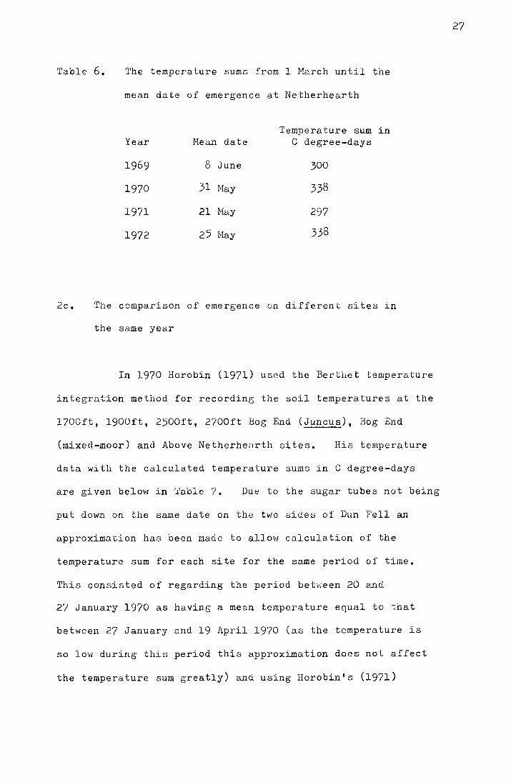
Table 6. 'I' he temperature sumc from l Me.rch until the

mean date of emergence at Netherhearth

Temperature sum in Year He an date C degree-days

1969 8 June 300

1970 31 Hay 338

1971 21 Hay 297

1972 25 t•lay 338

2c. The comparison of emergence on different sites in

the same year

In 1970 Horobin (1971) used the Berthet temperature

integration method for recording the soil temperatures at the

l700ft, l900ft, 2500ft, 2700ft Bog End (Juncus), Bog End

(mixed-moor) and. Above Netherhearth sites. His temperature

data with the calculated temperature sums in C degree-days

are given below in ~able 7. Due to the sugar tubes not being

put down on the same date on the h;o sides of Dun Fell an

approximation has been made to allow calculation of the

temperature sum for each site for the same period of time.

This consisted of regarding the period betv:een 20 and

27 January 1970 as having a mean temperature equal to that

between 27 January and 19 April 1970 (as the temperature is

so low during this period this approximation does not affect

the temperature sum greatly) and using Horobin's (1971)

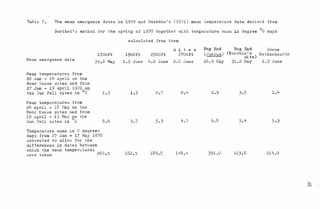
Table 7. The mean emergence dates in 1970 and Horobin's (19'71) mean temperature data derived from

Berthet's method for the spring of 1970 together with temperature sums in degree °C days

Mean emergence date 1700ft

29.8 May

Hean temperatures from 20 Jan - 24 April on the Hoar House sites and from 27 Jan - 19 April 1970 on the Dun Fell sites in °C

Mean temperatures from 24 April - 18 Eay on the Noor House sites and from 19 April - 13 May on the Dun Fell sites in °C

1.3

6.4

Temperature sums in C degree­days from 27 Jan - 13 May 1970 corrected to allow for the differences in dates between which the mean temperatures

269.3 \·Jere taken

calculated from them

1900ft

1.9 June

1.3

5.7

252.5

2500ft

4.2 June

0.7

5.3

189.5

.S i t e s 2700ft

6.6 June

0.4

4.7

148.4

Bog End (Juncus)

26.9 1-:!ay

2.9

6.8

391.0

Bog End Above (Horobin's Netherhearth

site) 31.2 May 1.3 June

3.5 1.4

5.4 5.3

413.8 214.0

1\) co

relationship between the mean obtained from the sugar inversion

method and that from the screen data to correct for the period

13 - 18 May 1970. 'l'he mean soil temperature for the period

13 - 18 May 1970, 8.97°C, has been obtained by the substitution

0 of the mean screen temperature of 7.4 C in the equation

y = o.87x - o.4, where y is the me~n in °C from the screen data

and x is the mean in °C obtained from the Berthet method. fhe

29

soil temperature has then been multiplied by five and 44.8Cdegree

- days have been subtracted from each temperature sum at the

Moor House sites. Table 7 gives the mean dates of emergence

at three Hoor House sites (the Bog J~nd mixed-moor 0i te used

by Horobin was close to, but approximately lOft above, my site

on the west facing slope) and the four Dun Fell cites.

Ilorobin's temperature data and the approximate temperature sums

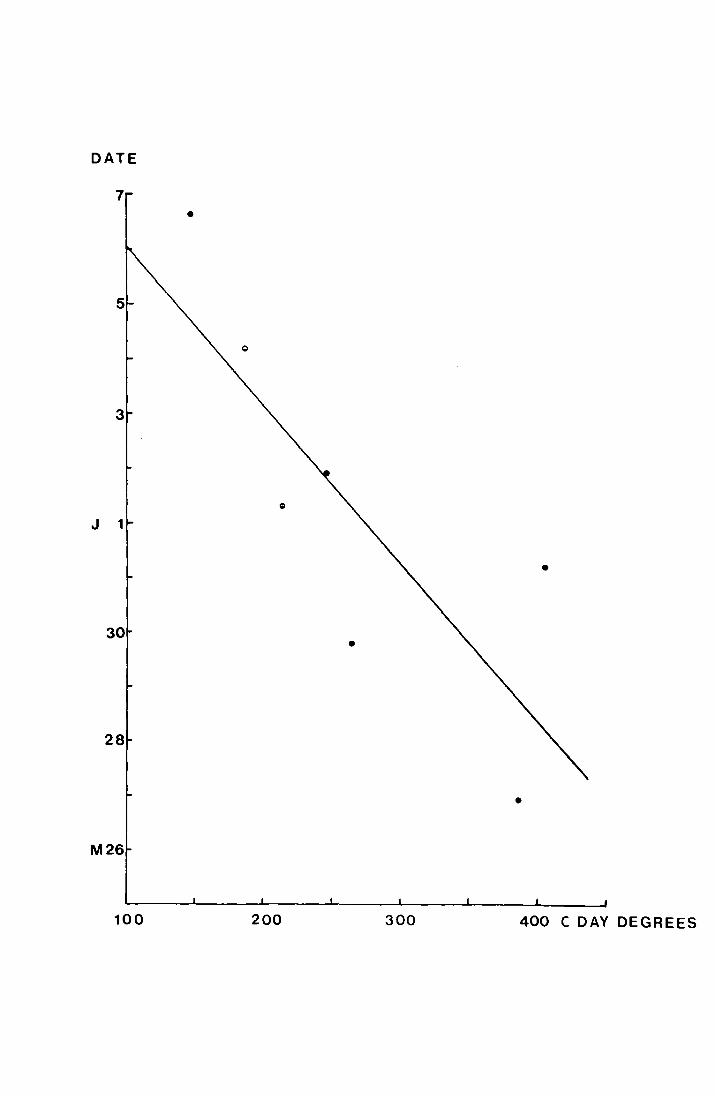
derived from them are sho~tm in the .c;ame table. In Fig. 12 the

mean date of emergence has been plotted against the temperature

sum bet,.1een 27 January and 13 Jviay 1970. 'rhiG gives the

equation y = 14.87 - 0.028x, where the correlation coefficient

is -0. 8 (9 9' p..:::: 0. 0 5. If the mean emergence date on each site

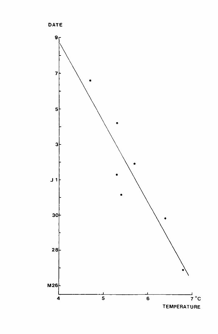
is plotted against the uncorrected mean tempe:ca.ture data for

April to mid May a correlation of r = -0.917, p <:: 0. 01. is

obtained ~nd the regression has the equation y = 32.53 - 4.46x.

This is shown in Fig. 13.

It is clear from these results that the mean emergence

date is closely correlated with spring temperature, but the

data do not indicate a constant temperature .sum from 27 January

to the mean date of emergence which was suggested by the results

from the year to year comparisons at Netherhearth.

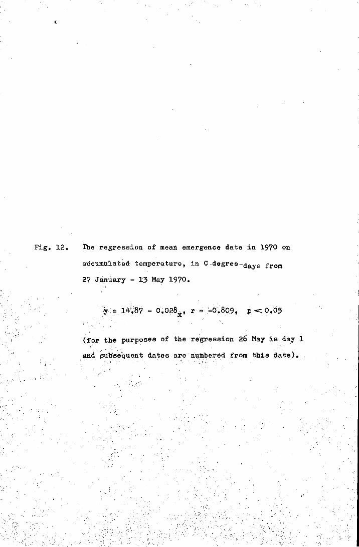
Fig. 12.

. . ~': ;

. , :·j . -· ~ . . -~ •,. , ;-_ .. ,:'r,

·.: - ,· ,·,. • I

, ·,,· I, ;•.,.

·.

-~ . '. .

The regression of mean emergence date in 1970 on

accumulated temperature, in C.degree-days from

27 J~uary - 13 ~Y 1970.

(:for the p1Jrposea of the·regression 26.r1ay is liay 1

. aild. Sll'bsequen t elates aro · n1.;1~1:>ered from this <late). . ' ·, •• ~ ' I ·~. ~ .. ~

.c

_.,-:· ..

. ·;.-

... . ' •• 1·

,;_ ': ,_

.. •:'

I ~ .__ '

... ,._,,

.. ; .. ·.·• . :. ·~. _· .

-... . " ___ .. :

,'

.c

'.-··· .·. .. ,

... '!, •• ,\,.

DATE

•

M26

100 200 300 400 C DAY DEGREES

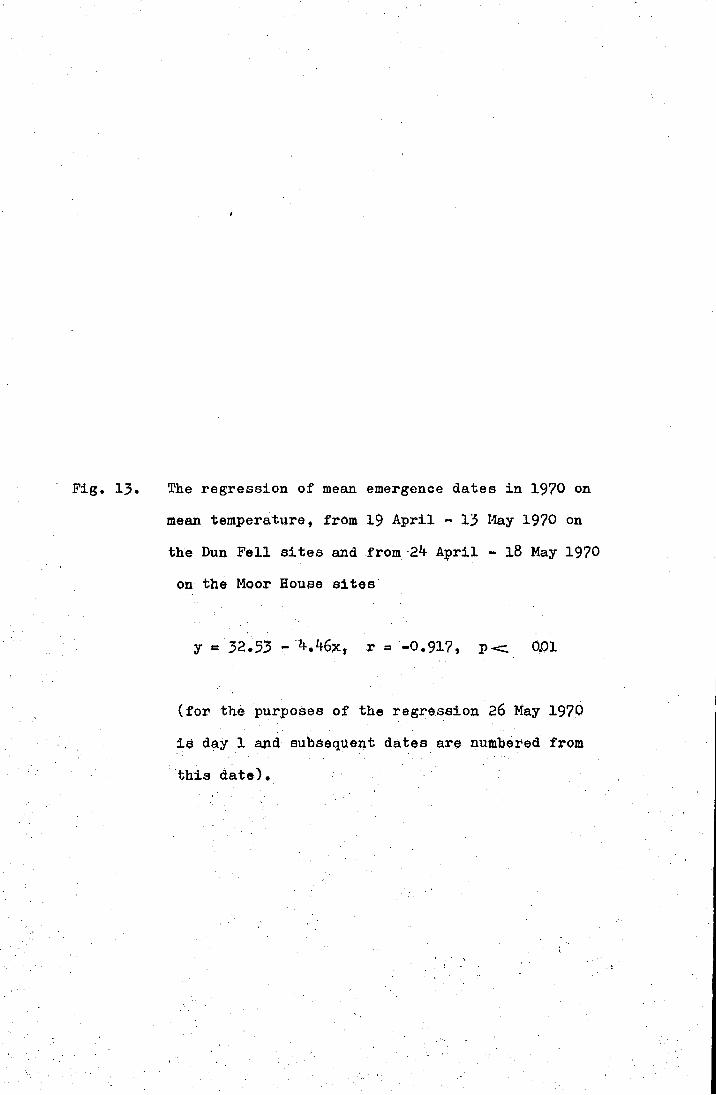
- Fig. 13. The regression of mean emergence dates in 1970 on

mean temperature, from 19 April - 13 Hay 1970 on

the Dun Fell sites and .from-24 April- 18 May 1970

on the Moor House sites

y = 32 • .53 - 4.46:xt r c -0.917, I><:. 0.01

(for the purpOI3eS of the regression 26 May 1970

iS day 1 and subsequent dates are numbered from

this date).

DATE

9

J 1

30

28

4

e

•

5 6 7°C TEMPERATURE

30

2d. Discussion

There are a number of reasons why, although development

is temperature dependent, the emergence date might not depend

on the accumulation of a specific temperature sum calculated

as C degree-days above 0°C. 0

In the first place, 0 C may not

be the threshold for development and development might continue

below or be discontinued at a higher temperature. Glenn (1922,

1931) therefore used "effective day degrees" \>Jhich \vere based

on the temperatures above the threshold for development. In

theory this threshold can be obtained graphically from

experimental resul t.s at consto.n t temperature~.:;. If the re.te

of development is plotted against temperature extrapolation

of the regression line back will cut the temperature axis at

the "developmental zero". In practice~as Krogh (1914) pointed

out, development usually continues at temperatures below this.

The second reason that temperature summation may not

give consistent results is linked to the first in that the

hyperbola is not usually the most appropriate description

of the relationship between development rate and temperature

(Andrewartha and Birch 195L~), and that this applies most

specifically in the region of the upper and lower development

thresholds. Before a predictive model for the relationship

between field temperatures and emergence de.te can be made,

information on the type of curve that is the best expression

of the relationship between development rate and temperature

is required. This is best found under constant temperature

conditions in the laboratory.

There is a further barrier to making accurate field

predictions in that, as Laughlin (1967) found, development

under field conditions may be 13.t a higher rate than predicted

from constant temperature experiments in the laboratory. It

has been suggested that this is the result of the fluctuation

of field temperature which in it~elf promotes development.

Since Andrewartha and Birch (1954) disputed this 0uggestion

there has been further work on this aspect (Messenger 1964)

which will be discussed when the laboratory studies on

T. subnodicornis are compared with the field results.

VI. The timing of emergence under controlled

temperature conditions in the laboratory

1. Culture Methods

Eourth instar larvae were cultured in crystallizing

dishes lOOmm in diameter and 45mm in depth on a bed of washed

sand approximately lcm in depth. 'l'he sand vias kept moist

and liverworts and Juncus litter were added as food which

was replaced when needed.

secured by a rubber band.

Each dish was covered by polythene

Between 10 and 20 larvae were put

in each dish and no problems of cannibalism arose.

Experiments were carried out either in constant

temperature cabinets of .07m3 capacity fitted with 8 watt

fluorescent tubes or in constant temperature roomsfitted

31

with 8 watt fluorescent tubes, Can 80 v1att ceiling li2;ht in the

15°C roomJ. Each light was wired in series with a "Venerette"

time switch so that the photoperiod could be controlled

automatically. The culture dishes were placed approximately

30cm below the 8 watt tubes in the cabinets and in the l0°C

and 5°C rooms and approximately 2m below the 80 watt tubes in

the l5°C room. In these positions they received illumination

of 150 - 240 lux.

32

On 29 February 1972, 95 larvae were obtained by Berlese

extraction of soil samples taken from the site behind the house.

A total of 32 larvae, in three cultures, were put in the l5°C

room, 42, in three cultures, in a cabinet at l0°C, and 21, in

two cultures, were put at 7°C in a cabinet. The temperatures

were monitored by thermographs and the cabinets were adjusted

frequently so that they rarely showed more than l°C divergence

from the desired temperature. In all three cases the light

regime was L : D, 18 : 6.

2. The effect of temperature on the development rate

in the stage before pupation

The mean dates of pupation at the three temperature

regimes are shown in Table 8 and the differences between means

are shown to be significant, using a t-test.

33

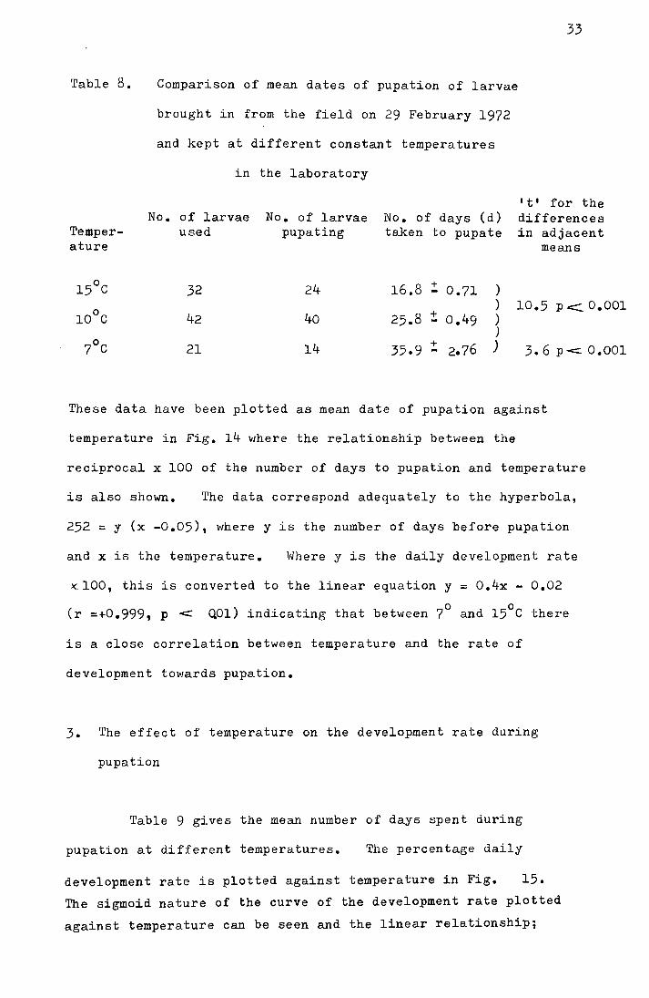
Table 8. Comparison of mean dates of pupation of larvae

brought in from the field on 29 February 1972

and kept at different constant temperatures

in the laboratory

Temper­ature

No. of larvae used

No. of larvae pupating

No. of days (d) taken to pupate

't' for the differences in adjacent

means

32 24 16.8 + 0.71 ) -

) 10.5 p < 0.001 + 42 40 25.8 0.49 )

)

21 14 35.9 +

2.76 ) 3.6 pc:::::: 0.001 -

These data have been plotted as mean date of pupation against

temperature in Fig. 14 where the relationship between the

reciprocal x 100 of the number of days to pupation and temperature

is also shown. The data correspond adequately to the hyperbola,

252 = y (x -0.05), where y is the number of days before pupation

and x is the temperature. Where y is the daily development rate

KlOO, this is converted to the linear equation y = 0.4x- 0.02

(r =+0.999, p ~ QOl) indicating that between 7° and l5°C there

is a close correlation between temperature and the rate of

development towards pupation.

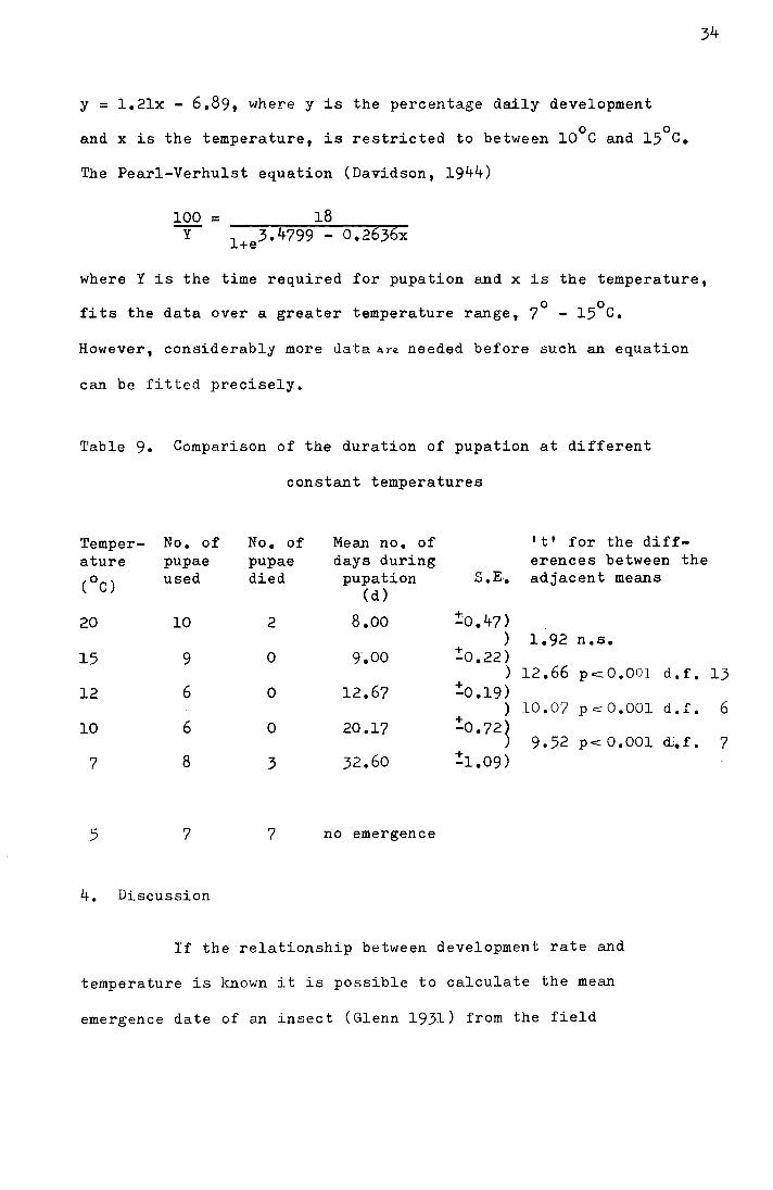
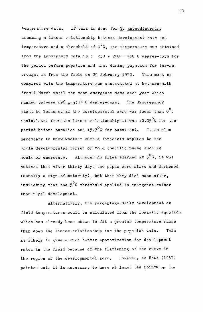
3. The effect of temperature on the development rate during

pupation

Table 9 gives the mean number of days spent during

pupation at different temperatures. The percentage daily

development rate is plotted against temperature in Fig. 15.

The sigmoid nature of the curve of the development rate plotted

against temperature can be seen and the linear relationship;

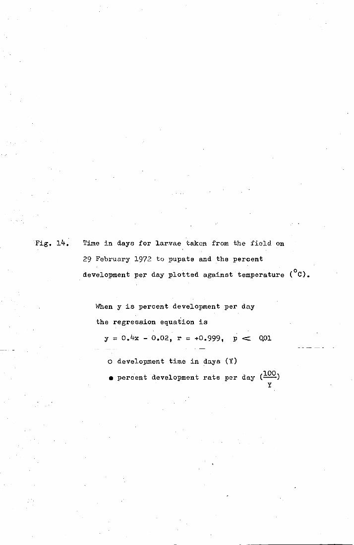
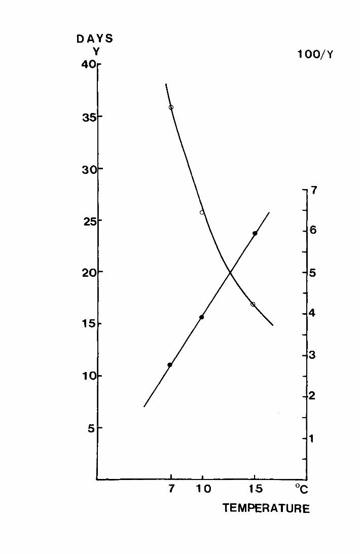
Fig. 14. Time in days for larvae taken from the field on

29 February 1972 to pupate and the percent

t d 1 d . t (°C). developmen per ay p otte aga~nst emperature

Hhen y is percent development per day

the regression equation is

y = 0.4x - 0.02, r = +0.999, p ~ QOl

o development time in days (Y)

• percent development rate per day (100 ) y

DAYS v

40

35

30

25

20

15

10

5

100/Y

7 10 15 °C

TEMPERATURE

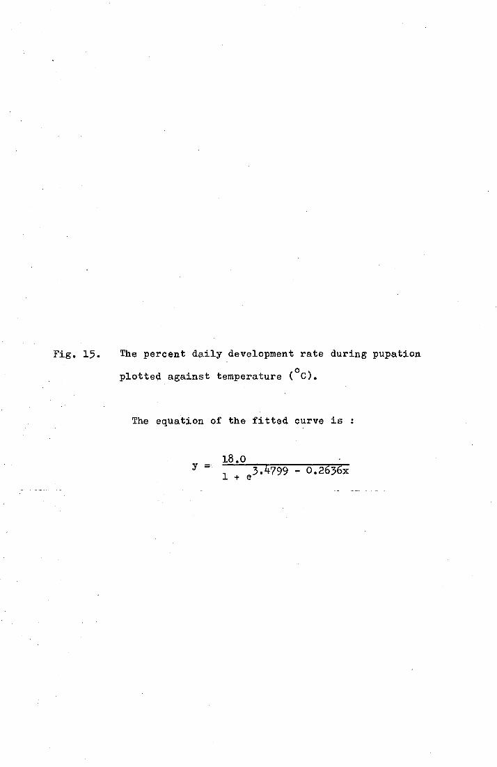
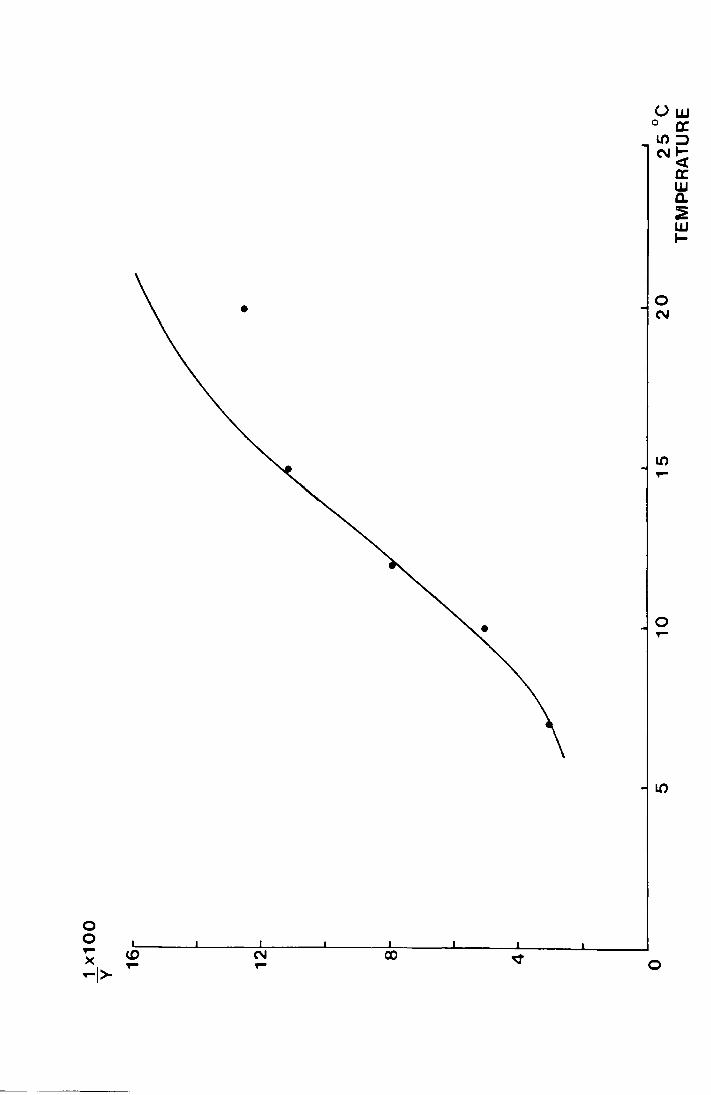
Fig. 15. The percent daily development rate during pupation

plotted against temperature (°C).

The equation of the fitted curve is

18.0 Y ;:

1 3.4799 - 0.2636x

+ e

0 0 .,.. <D >< .,.. -I>

Uw 0 cr. l():::J N~

0 N

Ll) ,....

0 ,....

0

cr w a. ~ w 1-

34

y = 1.2lx - 6.89, where y is the percentage daily development

0 0 and x is the temperature, is restricted to between 10 C and 15 c.

The Pearl-Verhulst equation (Davidson, 1944)

100 = y

18

where Y is the time required for pupation and x is the temperature,

f ·t th d t t t t 7°- 15°C. ~ s e a a over a grea er empera ure range,

However, considerably more data l\n needed before such an equation

can be fitted precisely.

Table 9. Comparison of the duration of pupation at different

constant temperatures

Temper- No. of No. of Mean no. of It I for the diff-ature pupae pupae days during erences between the

(oC) used died pupation s .E-. adjacent means (d)

20 10 2 8.00 :!:o.47 > ) 1.92 n.s.

15 9 0 9'.00 :!:o.22) ) 12.66 p c::::.O.OOl d. f.

12 6 0 12.67 :!:o.l9) ) 10.07 pcO.OOl d.f.

10 6 0 20.17 :0.72~ 9.52 p< 0,001 d). f.

7 8 3 32.60 :!:1.09)

5 7 7 no emergence

4. Discussion

If the relationship between development rate and

temperature is known it is possible to calculate the mean

emergence date of an insect (Glenn 1931) from the field

13

6

7

temperature data. If this is done for !· subnodicornis,

assuming a linear relationship between development rate and

0 temperature and a threshold of 0 C, the temperature sum obtained

from the laboratory data is 250 + 200 = 450 C degree-days for

the period before pupation and that during pupation for larvae

brought in from the field on 29 February 1972. 'l'his must be

compared with the temperature sum accumulated at Netherhearth

from l March until the mean emergence date each year which

ranged between 296 and338 C degree-days. 'I'he discrepancy

might be lessened if the developmental zero was lower than 0°C

0 (calculated from the linear relationship it was +0.05 C for the

period before pupation and +5.7°C for pupation). It is also

necessary to know ~tihether such a threshold applies to the

whole developmental period or to a specific phase such as

moult or emergence. Although no flies emerged at 5°C, it was

noticed that after thirty days the pupae were alive and darkened

(usually a sign of maturity), but that they died soon after,

0 indicating that the 5 C threshold applied to emergence rather

than pupal development.

Alternatively, the percentage daily development at

35

field temperatures could be calculated from the logistic equation

which has already been shown to fit a greater temperature range

than does the linear relationship for the pupation data. This

is likely to give a much better approximation for development

rates in the field because of the flattening of the curve in

the region of the developmental zero. However, as Howe (1967)

pointed out, it is necessary to have at least ten points on the

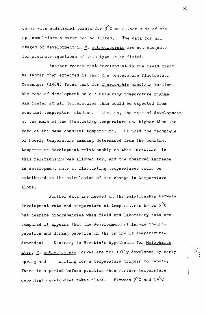
curve with additional pointB for 3°C on either side of the

optimum before a curve can be fitted. The data for all

stages of development in !· subnodicornis are not adequate

for accurate equations of this type to be fitted.

Another reason that development in the field might

be faster than expected is that the temperature fluctuates.

Messenger (1964) found that for Therioaphis maculata Buckton

the rate of development on a fluctuating temperature regime

was faster at all temperatures than would be expected from

constant temperature studies. That is, the rate of development

at the mean of the fluctuating temperature was higher than the

rate at the same constant temperature. He used the technique

of hourly temperature summing determined from the constant

temperature-development relationship so that curvature in

this relationship was allowed for, and the observed increase

in development rate at fluctuating temperatures could be

attributed to the stimulation of the change in temperature

alone.

Further data are needed on the relationship between

development rate and temperature at temperatures below 7°C

but despite discrepancies when field and laboratory data are

compared it appears that the development of larvae towards

pupation and during pupation in the spring is temperature-

dependent. Contrary to Horobin's hypothesis for Molophilus

ater, !· subnodicornis larvae are not fully developed by early

spring and waiting for a temperature trigger to pupate.

There is a period before pupation when further temperature

dependent development takes place. 0 0

Between 7 C and 15 C

a linear relationship describes the relationship between

development rate and temperature, but more data would probably

indicate that the logistic curve would be more appropriate,

especially at field temperatures. The rate of development

during pupation is also temperature dependent as it is in

~· ater (Hadley 197lb),and this relationship is also probably

best described by the logistic equation.

VII. 'fHE EFFECT OF TEMPERATURE ON THE RA'fE OF DEVELOPMEN'r

OF THE EGG AND OF TEMPERATURE AND PHOTOPERIOD ON THE

RATE OF DEVELOPIVJENT IN THE PRE-vliN'l'ER LARVAL .STAGES

Whether the linear or logistic relationship between

rate of development and temperature is used, in the middle part

of the favourable temperature range the development rate is

approximately linearly related to temperature. Danilevskii

(1965) shows that for a number of lepidopterous species the

development rate is directly related to temperature over the

temperature range encountered in the environment.

It has been suggested that in the spring the field

temperatures are below the range over which the development

rate of T. subnodicornis is linearly related to temperature.

This would diminish the effect of temperature differences

during this period but it is clear from the field data as well

as from the laboratory experiments thdt the timing of emergence

in spring is still positively related to temperature. As egg

d•evelopment and a large part of the larval development takes

place during the summer months when the mean temperature is

above 10°C, it would be expected that the rate of development

37

would be directly related to temperature during this period

and, unless a diapause intervenes or larvae are inhibited

from further development at some stage, an annual life-cycle

cannot be maintained under differing temperature conditions.

Accordingly, the response of egg development and larval growth

t t t t t t f 5 - 25°C has ra·e o cons an empera ure over a range rom

been examined in the laboratory. As photoperiod has also

been shown to have an effect on growth rate in certain cases

(Geyspitz and Zarankina 1963; Danilevskii 1965; Beck 1968)

it was also decided in 1972 to compare the effect of long day

L : D; 18 : 6, and short day L : D; 6 : 18, on the growth

of larvae in culture.

1. The relationship between temperature and egg development

rate

Nethod

Newly emerged males and females \vere allowed to

copulate in covered crystalli~ing dishes. A sheet of damp

crumpled tissue paper provided ridges from which the pair

could hang while copulating and kept the humidity high.

On the completion of copulation, decapitation of the females

ensured that the eggs were laid in quick succession (Coulson

1962) 0 These were picked up on the end of a brush and placed

on damp tissue paper in Petri dishes. The dishes were then

0 0 0 placed in constant temperature cabinets at 25 , 20 , 15 ,

Results

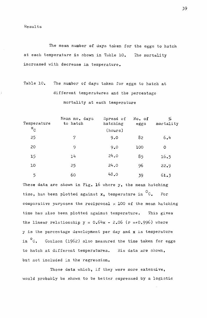
The mean number of days taken for the eggs to hatch

at each temperature is shown in Table 10. The mortality

increased with decrease in temperature.

Table 10. The number of days taken for eggs to hatch at

different temperatures and the percentage

mortality at each temperature

Hean no. days Spread of No. of % Temperature to hatch hatching eggs mortality

oc (hours)

25 7 9.0 82 6.4

20 9 9.0 100 0

15 14 24.0 85 16.5

10 25 24.0 96 22.9

5 60 48 .o 39 61.3

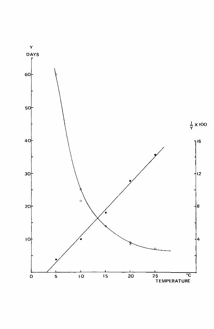
These data are shown in Fig. 16 uhere y, the mean hatching

time, has been plotted against x, temperature in oc. For

comparative purposes the reciprocal x 100 of the mean hatching

time has also been plotted against temperature. This gives

the linear relationship y = o.64x - 2.06 (r =-4-0.996) vlhere

y is the percentage development per day and x is temperature

0 in c. Coulson (1962) also measured the time taken for eggs

to hatch at different temperatures. His data are shown,

but not included in the regression.

These data which, if they were more extensive,

would probably be shown to be better expressed by a logistic

39

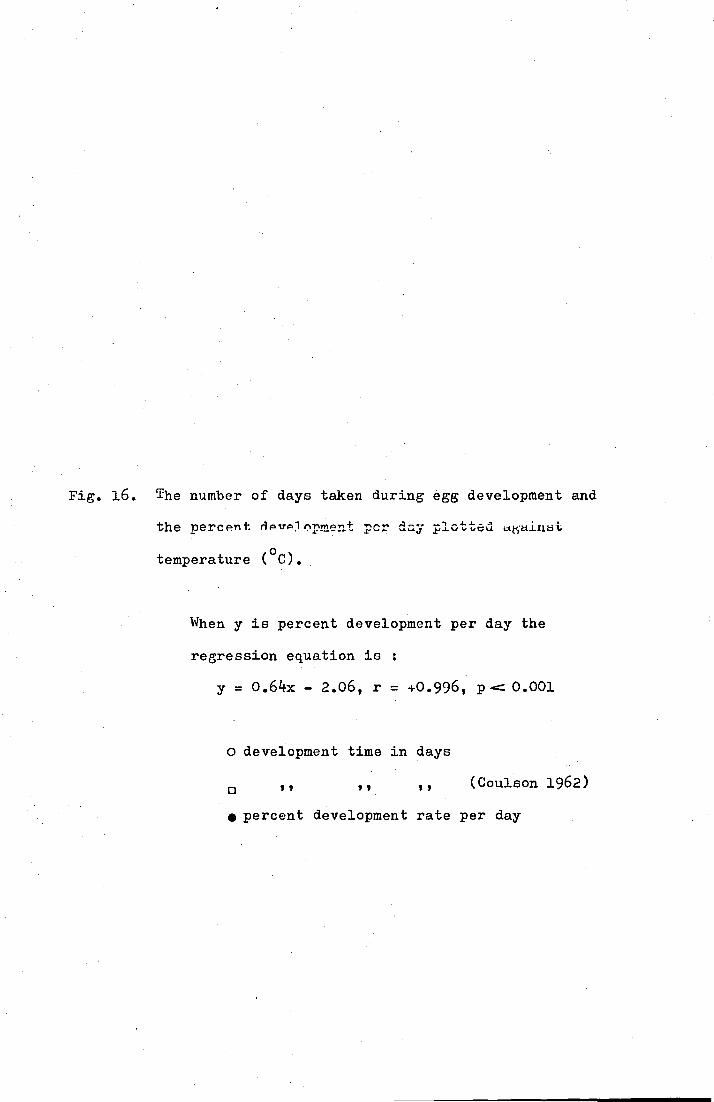
Fig. 16. The number of days taken during egg development and

t ( OC). emperature

When y is percent development per day the

regression equation is

y = o.64x - 2.06, r = +0.996, p <: 0.001

o development time in days

0 ' ' ' ' ' ' (Coulson 1962)

e percent development rate per day

y

DAYS

60

50

40

30

20

10

0 5 10 15 20

lx100 y

16

12

8

4

25 oc TEMPERATURE

curve correspond to the expected type of relationship between

development rate and temperature. Although there is probably

a departure from the linear relationship between development

0 0 0 rate and temperature at 5 C, between 7 C and 25 C the relation-

ship is close enough to be used predictively.

2. The effect of temperature on larval growth rates (1971)

2a. Method

During the emergence period in 1971 fertilised

females were gathered in the field and enclosed, on damp filter

paper, in crystallizing dishes. Under these conditions they

laid most of their eggs within 12 hours. The eggs were then

removed with a paint brush to damp filter paper in Petri dishes.

The Petri dishes were kept at l5°C until the larvae hatched.

On hatching, the first instar larvae were tr!illsferred

in groups of 20 to a culture medium of leafy liverworts on a

base of wet sand in Petri dishes, and on reaching about 20mg

the larvae were transferred to the same type of culture in

crystallizing dishes. The liverworts consisted largely of

Dyplophyllum albicans and Ptyllidium ciliare found around the

Juncus bases at Netherhearth. Twenty Petri dishes were put

at each of the following temperature regimes 0 0 0

25 ' 20 ' 15 '

In all cases the photoperiod regime was L : D,

18 : 6, and the cultures were arranged so that they received

the same amount of incident light (150- 240 lux). The

temperatures were monitored by Cambridge thermographs in

40

constant temperature rooms and by Castella thermohygrographs

in constant temperature cabinets. When working normally

neither the constant temperature rooms nor the cabinets

deviated by more than: l°C from the set temperature.

At intervals of two to four weeks, larvae were

taken from each of the sets of cultures and weighed.

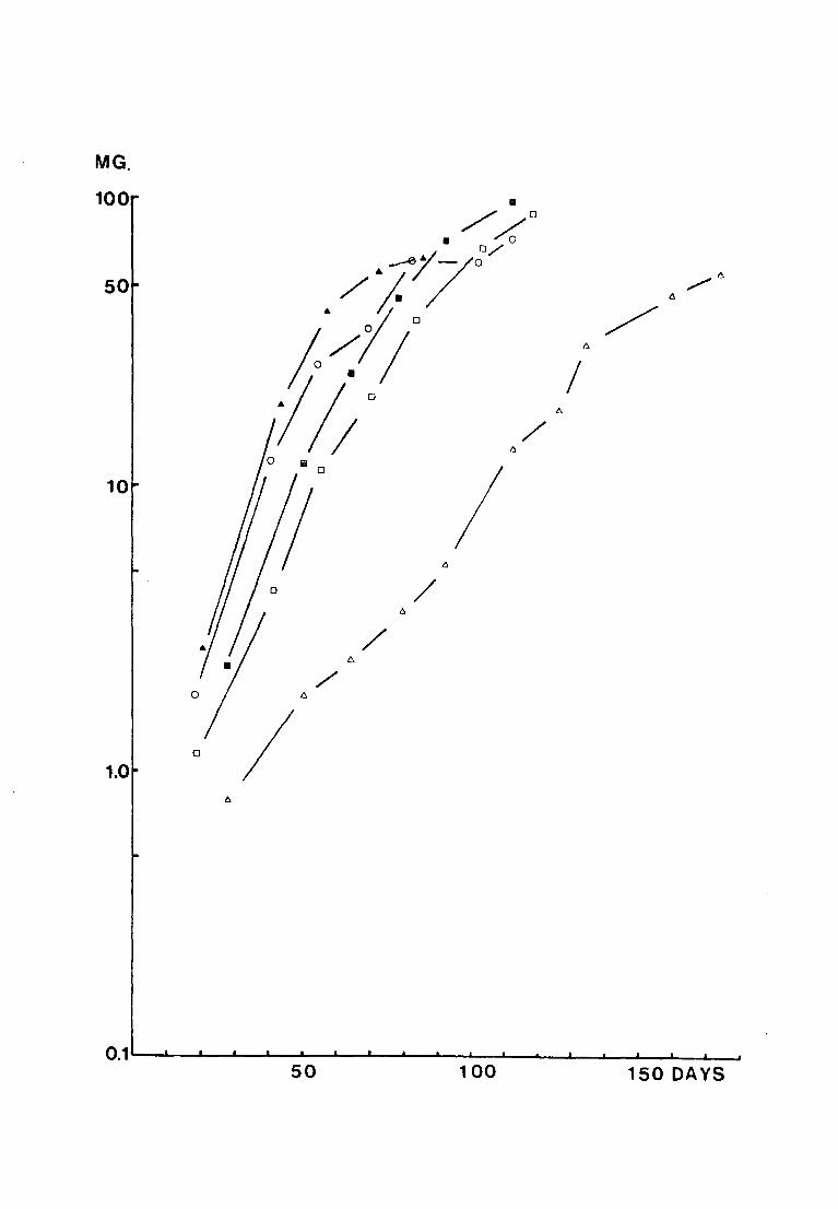
2b. Results

The mean weights of the larvae at each temperature

regime are shown in Table V in the appendix and plotted on a

logarithmic scale against time in Fig. 17. It appears that

0 2~0 c the growth rates at temperatures from 10 - v are not

positively related to temperature over the weight range from

0 The larvae kept at 25 C grew faster than at the 5 - 50mg.

other temperatures initially, but all larvae died before

5 October 1971 and the peru{ mean weight attained was 62.5mg,

0 as opposed to 97.8mg at 15 C.

Table ll shows the number of days and the daily

percentage rate of development at each temperature for the

range in weight from 5 - 50mg.

41

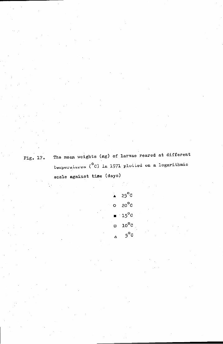
Fig. 17. The mean weights (mg) of larvae reared at different

.L -- I ,o,.., , ""'l"'r-"1""1 vt:mJJt:.L·c;t.L<~.lJ.·~-:::; \ vJ .1.11 .1./fJ. pluLLeu on a logarithmic

scale against time (days)

0

• 0

MG.

100

50

10

1.0

0

0

6

a

/ /(rJ • 0/0

./J.j7o /6

!:~;l~o 6

/ /)

I/; 0

I "

o I / Iii

1'.

0

I I "

/ "

/ 6.

/ 6

I

0.1-~~~~~ 100 150 DAYS

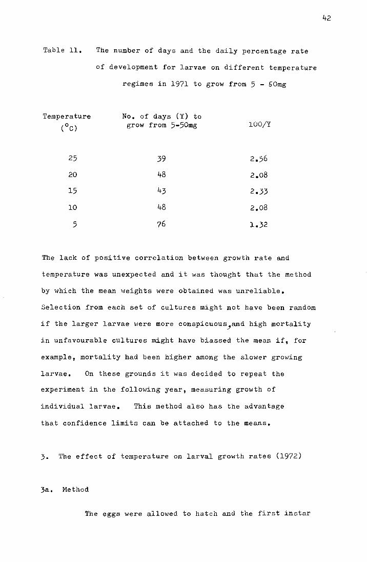
Table ll.

Temperature

(oC)

25

20

15

10

5

The number of days and the daily percentage rate

of development for larvae on different temperature

regimes in 1971 to grow from 5 - 50mg

No. of days (Y) to grow from 5-50mg

39

48

43

48

76

100/Y

2.56

2.08

2.33

2.08

1.32

The lack of positive correlation between growth rate and

temperature was unexpected and it was thought that the method

by which the mean weights were obtained was unreliable.

Selection from each set of cultures might not have been random

if the larger larvae \'Jere more conspicuous _,and high mortality

in unfavourable cultures might have biassed the mean if, for

example, mortality had been higher among the slower growing

larvae. On these grounds it was decided to repeat the

experiment in the following year, measuring growth of

individual larvae. This method also has the advantage

that confidence limits can be attached to the means.

3. The effect of temperature on larval growth rates (1972)

3a. Method

The eggs were allowed to hatch and the first instar

42

larvae were cultured as in 1971. The cultures were placed

under similar temperature and light conditions as before,

with the addition of another temperature regime, 7°C.

After a week, 20 larvae from each of the culture sets at

25°, 20°, 15° and 10°C were weighed and put in individual

cultures of liverwort on damp sand in standard 2 x l inch

tubes. 20 larvae from the 7°C regime were set up in similar

0 cultures the week after and 20 larvae from the 5 C regime the

following week. The larvae were weighed at approximately

0 0 10 day intervals, longer at 7 and 5 c, and on reaching 20mg

were transferred to 3 x 1~ inch tubes.

On 7 July 1972 two additional sets of cultures were

set up at 10° and 20°C respectively, on a photoperiod of

L : D, 6 : 18. The larvae used to start these cultures

0 0 were obtained fro1n the stock cultures at 10 and 20 C on

the L : D, 18 : 6 photoperiod.

In all cultures the medium was renewed at irregular

intervals whenever the food supply appeared to be less than

abundant or to be fouled. Dead larvae were replaced by

larvae from the stock cultures kept at each temperature

and photoperiod.

3b. Treatment of 1972 results

Few of the original larvae in each set of cultures

survived to pupate so it was decided to use the mean weight

increments rather than actual weights for analysis. However,

44

Figs. 18 and 19 showing mean weight of larvae,grown at the

photoperiod L : D, 18 : 6 and on different temperature regimes,

plotted arithmetically and logarithmically respectively against

date,are included for comparison with Fig. 17. 'l'he results

are similar in that there appears to be little difference in

the mean growth rates of larvae at temperatures between 10°

0 The larvae at 25 C failed to survive beyond three

weeks, possibly because of the malfunction of the thermostat

0 which allowed the temperature to rise to 28 C during this period.

Laughlin (1960) found that in T. oleracea the growth

curve was logarithmic during the first three instars and

arithmetic in the fourth. In Fig. 20 the mean weights of

a group of larvae on the L : D, 6 : 18 photoperiod and 10°C

regime that survived to reach their maximum weights have been

plotted against time. This shows that an initial logarithmic

growth phase is follo\'Jed by an ari thmet -·ic phase and that the

change takes place between 10 and 20mg. In order to find

whether this corresponded to a change in instar a small sample

of larvae was weighed and assigned to instar by measurement

of the spiracular disc (Coulson 1962). This is shown in

Fig. IV and Table VI in the appendix and it appears that,

as in !· oleracea, the change from logarithmic to an arithmetic

growth rate occurs at the change from the third to fourth instar

in the 16 - 25mg range. Accordingly, the weight of 20mg has

been regarded as the division between third and fourth instar

and increments of larvae weighing less than 20mg have been

compared as the mean logarithmic daily weight increment and

Fig. 18. The mean weights (mg) of larvae reared at different

i-t:!ID!ltll·at.ureo (°C) but the same photoperJ.od (L:JJ; J.8:6)

in 1972 plotted against time (date)

o 20°C

• 15°C

0 10°C

• 7°C

t:. 5°C

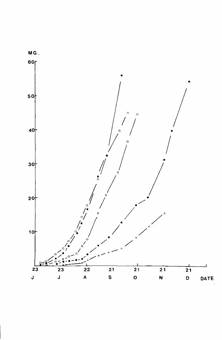
MG.

60

50

40

30

20

10

23

J

• •

0 0

/j •

V" I •

! •

0

~;

/0 • 0 I / •

0~· 0 / 6

~-I . / I ~ 6

o. / j . 6

/~ 0/0 ./ /

ol I / 6

/. 0 / 6--

0/ - • 6

/• o .... o ·-•" 6/ 0;:..--' 0-.-.- ... o-: ----- •.,. _ -6

23 22 21 21 21 21

J A s 0 N D DATE

Fig. 19. The mean weights (mg) of larvae reared at different

0 temperatures ( C) and the same photoperiod (L:D; 18:6)

in 1972 plotted on a logarithmic scale against time (date).

0 20°0

• 15°0

D 10°0

• 7°C

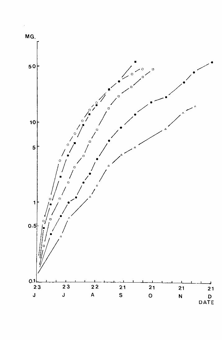
MG.

so

10

5

23

J

22 A

21

s 21

0 21

N

I J

21

D DATE

Fig. 20. The mean weight (mg) of eight larvae kept at 10°C

and a photoperiod of L:D; 18:6 in 1972 plotted on

a logarithmic scale against temperature.

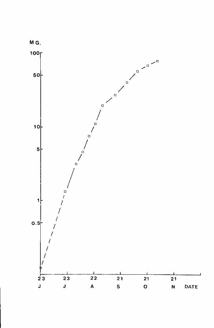
MG.

100

,.......o _.....o

0

50 / 0

/ 0

/ 0

I 10 I

0

0

5 I 0

I 0

I 0

I 1 I

I I

o.s I

I I

I I

I

23 23 22 21 21 21

J J A s 0 N DATE

45

increments of larvae weighing more than 20mg have been compared

as mean daily weight increments, all the original weighings

being in mg.

From Fig. 19 it appears possible that there are

inflections in the growth curves other than at 20mg. This

might have been an artifact produced by the substitution of

0 0 0 larvae, but at 20 , 7 and 5 C there is an inflection at 3mg

and this corresponds to the approximate \veight at which larvae

enter the third instar. So another division into Height

ranges has been made at this point and the increments of larvae

below 3mg are considered separately from those above. The

3 - 20mg range has been further divided into 3 - lOmg and

10 - 20mg ranges so that fourth instar or third instar larvae,

in which the growth rate was slowing as a prelude to moult,

are restricted to the heavier weight range.

From comparison of Figs. 18 and 19 it appears possible

that the arithmetic growth phase was entered earlier at higher

temperatures than at lower. In this case the logarithm of the

increment would be negatively correlated with weight and would

require correction. Table VII in the appendix shows the

regression parameters for the regressions of the logarithm

of the weight increment on the logarithm of the weight in mg.

It can be seen that in a number of cases there is a significant

though small regression coefficient. The data for the 10°C,

L : D; 18 : 6 regime in the 10 - 20mg range have been corrected

to allow for the negative relationship between the logarithms

of increment and original weight. This has had the result of

changing the mean logarithmic increment multiplied by 105 from

1581 : 200 to 1598 ! 206. As this is a difference of 1.1%

and not significant, it was decided that it \.,ras unnecessary

to make this type of correction.

46

An analysis of variance, shown in 'rable VIII in the

appendix, indicated that within each weight range the variation

between the weight increments of one larva was no less than

that between larvae. It was therefore decided to use all the

available weight increments of each larva in each weight range.

Death of larvae is usually preceded by loss of weight.

In order to eliminate this variation only the increments of

larvae that entered the weight range above that being considered

have been used. In the case of larvae weighing more than 20mg

the increment for the weight before the maximum weight and

subsequent increments have not been used.

3c. Results

'l'able 12 shows the mean of the logarithmic daily

increments for the weight ranges below 20mg and the mean

daily increments for weight ranges above 20mg for the larvae

grown under different temperature conditions, but at the

same photoperiod, L D; 18 : 6. Survival of larvae at

0 5 C was so low that only one set of data, that from the

0.12 - 3mg range, was available. The data have been

examined in two ways; first, the differences in growth

rate of larvae growing at each temperature have been compared

in each weight range to see whether the growth rate decreases

as the weight increases. Secondly, the growth rates at the

different temperature regimes have been compared within

each weight range. Students' t-test is used to indicate

the significance of the differences.

Table 13 shows that at each temperature there is a

significant drop in the logarithmic rate of growth between

the first and third weight ranges and that the decrease in

0 rate is greatest at 20 C. At the two higher temperatures,

0 0 but not at 7 or 10 C, the decrease in rate between the

0.12 - 3mg and the 3 - lOmg ranges is significant.

Table 14 shows the differences between rates in

the same weight range but at different temperatures. In

the 0.12 - 3mg range the rate is positively related to

temperature from 5 - 20°C but only the differences between

7° and 10°C and between 10° and 15°C are significant. In

the 3 - lOmg range the rates have decreased and none of the

differences between increments gained at adjacent temperatures

are significant. However, the rates are positively related

0 to temperature over the range from 7 - 20 C and the difference

between the rate at 7°C and the rate at 15°C is significant.

In the 10 - 20mg range the rate at 20°C drops below that at 0

15 C and the difference becomes significant in the range above

20mg. In this range the differences in growth rates between

7° and 15°C have d d t th ecrease o e extent that none of them

is significant.

47

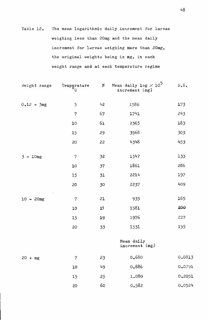
48

'fable 12. The mean logarithmic daily increment for larvae

weighing less than 20mg and the mean daily

increment for larvae weighing more than 20mg,

the original weights being in mg, in each

weight range and at each temperature regime

l.veight range Temp5rature N Mean daily log X 105 .S.E. c increment (rug)

0.12 - 3mg 5 42 1586 173

7 67 1741 243

10 61 2365 183

15 29 3568 303

20 22 4348 453

3 - lOmg 7 32 1347 133

10 37 1861 286

15 31 2214 197

20 30 2237 409

10 - 20mg 7 21 935 165

10 l? 1581 ,00 15 19 1976 227

20 33 1531 155

Mean daily increment (mg)

20 + mg 7 23 o.68o 0.0813

10 49 o.886 0.0791

15 25 1.080 0.2051

20 60 0.582 0.0524

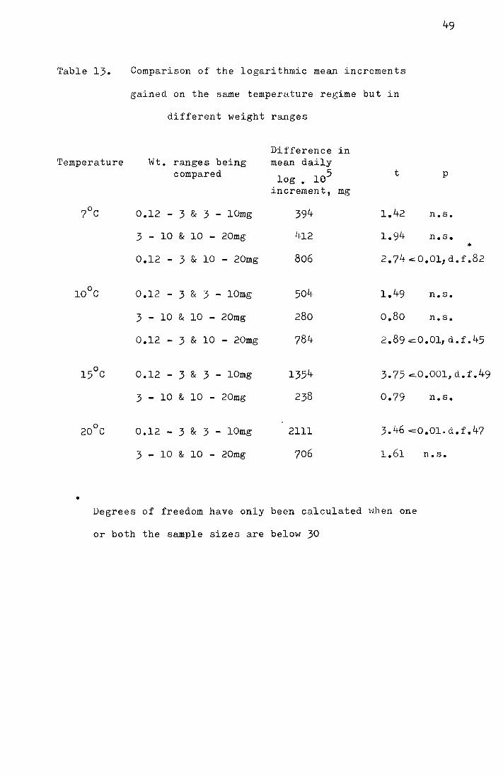
49

Table 13. Comparison of the logarithmic mean increments

gained on the same temperature regime but in

different weight ranges

Difference in Temperature Wt. ranges being mean daily

compared log • le5 t p

increment, mg

7°C 0.12 - 3 & 3 - lOmg 394 1.42 n.s.

3 - 10 & 10 - 20mg 412 1.94 n.s. •

0.12 - 3 & 10 - 20mg 806 2.74c::.O.Ol1 d.f.82

l0°C 0.12 - 3 & 3 - lOmg 504 1.49 n.s.

3 - 10 & 10 - 20mg 280 o.8o n.s.

0.12 - 3 & 10 - 20mg 784 2.89 ~o.o1, d.f.45

l5°C 0.12 - 3 & 3 - lOmg 1354 3.75 .:::.O.OOl,d.f.49

3 - 10 & 10 - 20mg 238 0.79 n.s.

20°C 0.12 - 3 & 3 - lOmg 2111 3.46 =O.OLd.f.47

3 - 10 & 10 - 20mg 706 1.61 n.s •

• Degrees of freedom have only been calculated ~1en one

or both the sample sizes are below 30

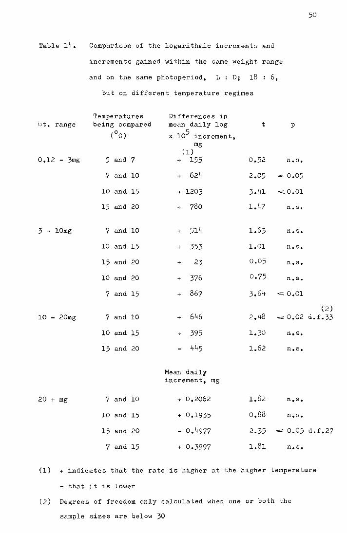
Table 14.

Ht. range

0.12 - 3mg

3 - lOmg

10 - 20mg

20 + mg

Comparison of the logarithmic increments and

increments gained within the same v1eigh t range

and on the same photoperiod, L D; 18 : 6,

but on different temperature regimes

Temperatures being compared

(oC)

5 and 7

7 and 10

10 and 15

15 and 20

7 and 10

10 and 15

15 and 20

10 and 20

7 and 15

Differences in mean daily log

x 105 increment, mg

(1) + 155

+ 624

+ 1203

+ 780

+ 514

+ 353

+ 23

+ 376

+ 867

t

0.52

3.41

1.47

1.01

0.05

0.75

3.64

p

n.s.

<- o.o1

n.s.

n.s.

n.s.

n.s.

n.s.

<:::::0.01

50

7 and 10 + 646 (2)

2.48 c:::::: 0.02 d. f.33

10 and 15

15 and 20

7 and 10

10 and 15

15 and 20

7 and 15

+ 395

445

Mean daily increment, mg

+ 0.2062

+ 0.1935

- 0.4977

+ 0.3997

1.30

1.62

1.82

n.s.

n.s.

n.s.

o.88 n.s.

2.35 -c:::: 0.05 d.f.27

1.81 n.s.

(l) + indicates that the rate is higher at the higher temperature

- that it is lower

(2) Degrees of freedom only calculated when one or both the

sample sizes are below 30

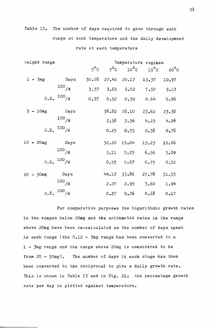
51

Table 15. The number of days required to grow through each

range at each temperature and the daily development

rate at each temperature

v~eight range Temperature regimes

5°C 7°C 10°C l5°C 20°C

1 - 3mg Days 30.08 27.40 20.17 13.37 10.97

100/d 3.37 3.65 5.02 7.57 9.23

S.E. 100/d 0.37 0.52 0.39 0.64 0.96

3 - lOmg Days 38.82 28.10 23.62 23.38

100/d 2.58 3.56 4.23 4.28

S.E. 100/d 0.25 0.55 0.38 0.78

10 - 20mg Days 32.20 19.04 15.23 19.66

100/d 3.11 5.25 6.56 5.09

s.E. 100/d 0.55 o.67 0.75 0.52

20 - 50mg Days 44.12 33.86 27.78 51.55

100/d 2.27 2.95 3.60 1.94

s.E. 100/d 0.27 0.26 o.68 0.17

For comparative purposes the logarithmic growth rates

in the ranges below 20mg and the arithmetic rates in the range

above 20mg have been re-calculated as the number of days spent

in each range (the 0.12 - 3mg range has been converted to a

1 - 3mg range and the range above 20mg is considered to be

from 20 - 50mg). The number of days in each stage has then

been converted to the reciprocal to give a daily growth rate.

This is shown in Table 15 and in Fig. 21; the percentage growth

rate per day is plotted against temperature.

Fig. 21. The percent growth rate per day for larvae in

four weight ranges plotted against temperature.

Upper left 1 - 3mg range Upper right 3 - lOmg range

Lower left 10 -20mg range Lower right 20 - 50mg range

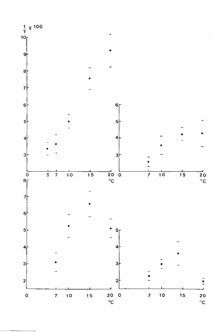
1 X 100 y

10

9

8

7

6

5

0 8

7

6

5

4

3

2

0

•

•

• •

5 7 10 1 5

•

•

•

7 10 15

•

6

5

20 0 oc

• 5

4

3

2

20 0 oc

•

7

•

7

• •

•

10 15 20 oc

•

•

•

10 15

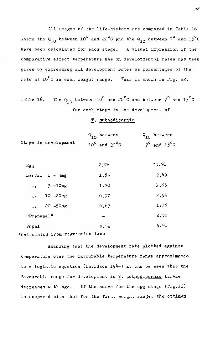
52

All stages of the life-history a.re compared in Table 16

where the Q10

between 10° and 20°C and the Q10

between 7° and 15°C

have been calculated for each stage. A visual impression of the

comparative effect temperature has on developmental rates has been

given by expressing all development rates as percentages of the

rate at 10°C in each weight range. 'l'his is shown in Fig. 22.

Table 16. The Q10

between 10° and 20°C and between 70 and 15°C

for each stage in the development of

T. subnodicornis

Stage in development

Egg

Larval 1 - 3mg

' ' 3 -lOmg

' ' 10 -20mg

' ' 20 -50mg

"Prepu]Dal 11

QlO

10°

between

0 and 20 C

2.78

1.84

1.20

0.97

0.67

Pupal 2.52

*Calculated from regression line

QlO

70

between

and 15°C

*3.91

2.49

1.85

5.91

Assuming that the development rate plotted against

temperature over the favourable temperature range approximates

to a logistic equation (Davidson 1944) it can be seen that the

favourable range for development in T. subnodicornis larvae

decreases with age. If the curve for the egg stage (Fig.l6)

is compared with that for the first \'>'eight range, the optimum

Fig. 22. The daily development rate at each temperature ---- -o

expressed as a percentage of the rate at 10 C

for a number of stages in the life-history.

• egg

ll. pupa

o 1- 3mg

• 3-lOmg

0 10-20lng

• 20-50mg

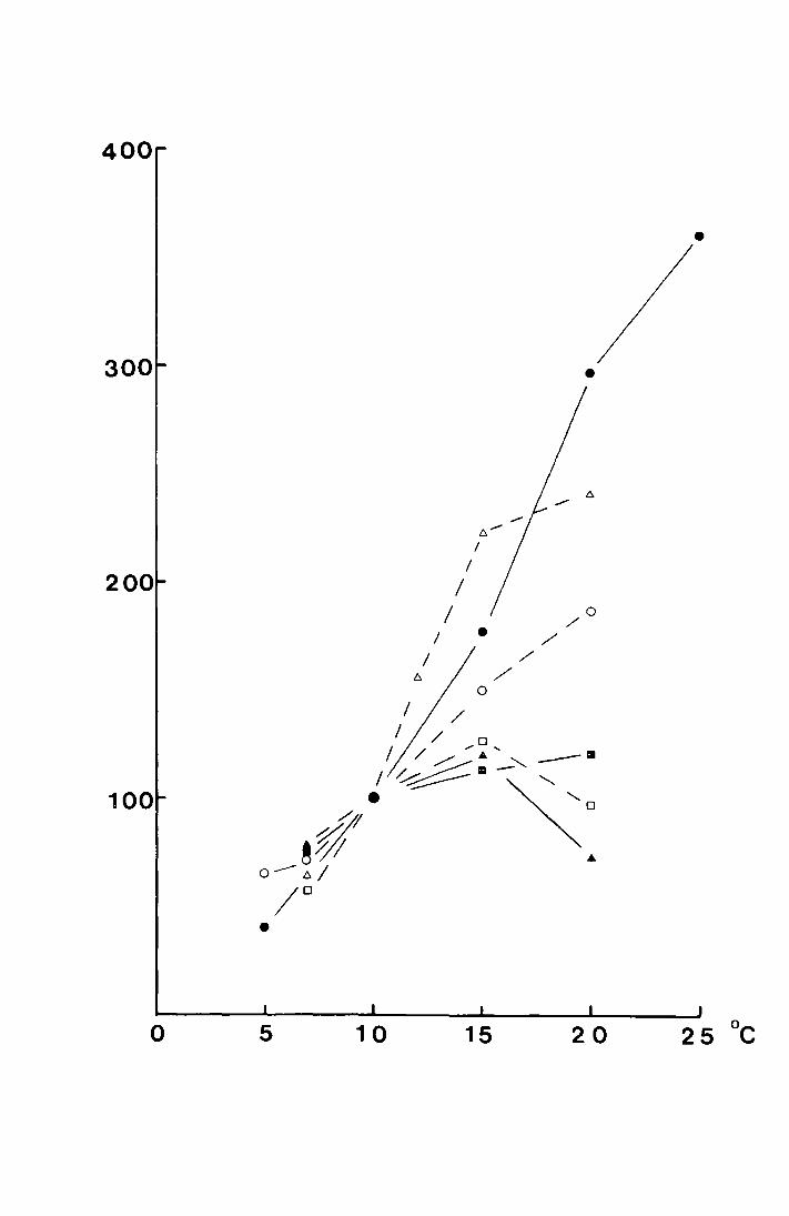
400

300

200

100

0

•

5 10

I

I •

/ /

0

15

/

•

0 /

20

•

temperature appears to have dropped. There are insufficient

data to estimate the positions of the optima in either case

but hatching of eggs occurs at 25°C whereas survival of larvae

is very low at this temperature. In the 3 - lOmg range the

optimum has dropped further and in the 10 - 20mg and 20 - 50mg

0 ranges it can be seen to be below 20 C. The lower limiting

53

0 temperature appears to be approximately 5 C throughout development.

Hatching and pupation, but not emergence, can take place at 5°C

and mortality in the larval stages at this temperature is high.

The decrease in favourable temperature range during development

is consistent with the results for Rhyzopertha dominica Fab. and

Calandra oryzae L. (Birch l945c) and may well be a more general

feature of insect development. Andrewartha and Birch (1954)

point out that there is no reason to suppose all stages in

development have the same temperature optima and that, as

they often take place under widely different environmental

temperature conditions, this would be unlikely.

3d Discussion

The extent of the favourable developmental range

and the positions of its upper and lower limits are related

to the life-history and habitat of an insect as well as to

the metabolic requirements inherent in biochemical reactions.

In a multivoltine insect living in temperate latitudes it is

important that the high summer temperatures should be fully

utilised and it would be expected that an insect such as

Pieris brassicae L. (Danilevskii 1965) would develop most

54

rapidly at comparatively high temperatures. It would also be

expected that their response to rise in temperature, manifested

by increase in growth rate, would be great.

In a univoltine insect without a diapause, and

relying on a synchronised emergence period, it would be an

advantage for the response to temperature, and the range over

which the response is made, to be small. During the life-

history of _!. subnodicornis there is a low optimum temperature

and a comparatively narrow favourable range for development.

Another feature of adaptive significance is the

decrease in the differences between growth rates at differant

temperatures within the favourable temperature range during

development. This is reflected in the drop in Q10 throughout

larval development. From Table 16 it can be seen that the

Q10

between 10° and 20°C declines throughout the embryonic

and larval growth period. This is also true for the Q10 0 0

between 7 and 15 C except in the 3 - lOmg range where it

can be seen from Fig. 22 that the growth rate at 15°C is

lower than would be expected. 'l'he decrease in Q10

during

larval development may also be common in insect development.

Geyspitz and Zarankina (1963) comment on this feature in the

development of Dasychira pudibunda L. reared at different

temperatures, and in T. subnodicornis it has the effect that

for the greater part of the life-history the development rate

responds only slightly to rise in temperature.

It appears that the development of !· subnodicornis

is adapted so that the temperature differences in the environment

will, for the greater part of its life-cycle, have little effect

on the development rate and therefore on the timing of the life-

history. This partly explains how the annual life-cycle

can be maintained over a considerable range of latitude

and altitude. However, as the Q10

for the temperature

0 range from 7 - 15 C, which approximates to the range of

mean daily temperatures at Moor House during the summer,

is above unity for most of the development period, these

adaptations cannot account fully for the degree of synchrony

shown in the life-cycle.

4. The effect of photoperiod on growth rate

Results

Table 17 shows the mean logarithmic daily weight

gains in the ranges below 20mg and the mean daily weight gains

for larvae above:- 20mg at 10° and 20°C on photoperiods of

L : D; 18 6, and L : D; 6 : 18. Student's t-test has

been used to test the significance of the differences in

growth rates between the two photoperiod regimes.

The differences between the growth rates on the

two photoperiod regimes are only significant on two occasions

55

in the •veight range above 20mg at.20_oC and in-the O.l2-3mg range

0 However, except in the 10 - 20mg range at 10 C,

the growth rate is faster at both temperatures on the short

day regime.

in the 0.12

The significant difference between the rates

3mg range at l0°C might be due to the effect

of new culture media on the larvae set up on the L : D; 6 : 18

regime; but the increased growth rate in the fourth instar on

the short day regime at 20°C, supported by a similar but not

significant increase at l0°C, may be a response to short

photoperiod.

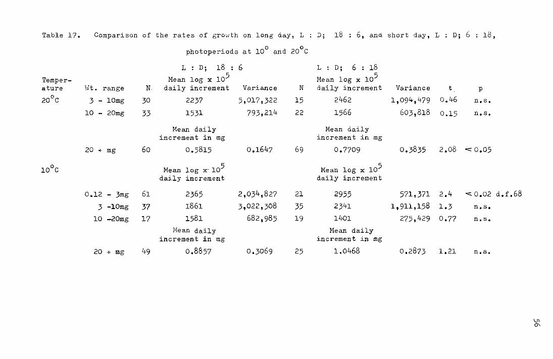
Table 17.

Temper­ature

20°C

10°C

Comparison of the rates of growth on long day, L : D; 18 6, and short day, L D; 6 18,

Ht. range

3 - lOmg

10 - 20mg

20 + mg

0.12 - 3mg

3 -lOmg

10 -20mg

20 + mg

photoperiods at 10° and 20°C

L : D; 18 : 6

Mean log x 105 N. daily increment Variance

30

33

60

61

37

17

49

2237

1531

Mean daily increment in mg

0.5815

Nean log x-105

daily increment

2365

1861

1581

Nean daily increment in mg

0.8857

5,017,322

793,214

0.1647

2,034,827

3,022,308

682,985

0.3069

N

15

22

69

21

35

19

25

L : D; 6 : 18

Hean log x 105

daily increment

2462

1566

Mean daily increment in mg

0.7709

Mean log x 105

daily increment

2955

2341

1401

Mean daily increment in mg

1.0468

Variance t

1,094,479 0.46

603,818 0.15

p

n.s.

n.s.

0.3835 2 .o8 c:::::: o.o5

571,371 2.4 ~0.02 d.f.68

1,911,158 1.3 n.s.

275,429 0.77 n.s.

0.2873 1.21 n.s.

\Jl 0"\

This experiment needs to be repeated starting the

cultures on the different photoperiods at the same date

and, as far as possible, with larvae of the same starting

weight. However, it appears likely that short day length

promotes growth in fourth instar larvae. Such a response

to photoperiod might affect larvae in the field that have

not completed their growth by the winter.

Discussion

The mechanism by which day length affects growth rate

is not clear. The simplest explanation is that a feeding

rhythm which corresponds to dark, as does that of Barathra

brassicae L. (Danilevskii 1965), or light, is prolonged by

the extension of the appropriate phase. Larvae of Agrostis

occulta L. (Danilevskii 1965), for instance, grow fastest and

have the shortest larval development time on continuous

illumination. Growth rate drops and development time grows

longer as day length is decreased. However, this type of

relationship does not always hold as Geyspitz. and Zarankina

(1963) have shown in their study on Dasychira pudibunda.

Here the growth rate was at a maximum between 3 and 6hrs

and a minimum at l6hrs daylight. Between 3 and Ohrs light

there was a considerable drop in the growth rate indicating

that a more complex reaction than a feeding response triggered

by darkness was taking place.

From the experimental results for T. subnodicornis it

0 can be seen that the larvae on the L : D; 6 : 18 at 10 C

photoperiod were growing at the same rate as those on the

57

58

L : D; 18 : 6 photoperiod at 15°C and it is suggested that

the short photoperiod might, in the field, compensate to a

certain extent for the drop in temperature in the autumn.

If the increase in growth rate were a response involving the

feeding rhythm, the increased rate of development would apply

only to those larvae that were still growing. Those that had

achieved maximum weight would be unaffected, so the response

to photoperiod might provide a mechanism by which larvae

growing in colder habitats could complete their growth by

the onset of winter.

5. The effect of temperature on larvae taken from the

field in the autumn

One further investigation into the temperature effect

was carried out on late fourth instar larvae in 1972.

~~enty larvae were taken from the field on 14 November

0 1972 and cultured at 15 c. On 28 November another twenty were

collected and these were put at 10°C. Both sets of larvae were

kept on a photoperiod of L D; 6 18 until 14 December 1972

when they were transferred to an L D; 18 6 photoperiod atl~C.

The photoperiod change was made in order to bring about rapid

and synchronised pupation which only occurs on long day length.

This reaction is discussed in the next section.

Results

Fourteen flies emerged from each culture. Those

that had been on the 15°C regime pupated at a mean of 24.8

! 1.3 days after the transfer to long photoperiod and the

59

0 larvae that had been on the 10 C regime pupated at a mean of

20.8 : 1.0 days after the transfer. The individual pupation

dates are shown in Table IX in the appendix. This result

indicates that from late November T. subnodicornis development

is not positively correlated with temperature when the larvae

are kept on a short photoperiod. The difference in the two

means (t = 2.44, d. f. 24, p c::::. 0.02) shows that there is a

slight (20%) retardation effect at the higher temperature.

Conclusion

The observations outlined above are of a very

preliminary nature and the experiment needs to be repeated

with larger numbers of larvae and over a range of temperatures;

however, it appears possible that when growth has been completed

T. subnodicornis larvae may go through a stage where development

is temperature independent or possibly, as is often the case in

diapause, continues at a faster rate at lower temperatures.

In this it resembles Phyllopertha horticola L. (Laughlin 1963)

which, although it also has a winter diapause, enters an

apparently temperature independent phase in the third instar.

The concept of diapause and "diapause development"

will be discussed later when the relationship between photoperiod

and development in the fourth instar is examined.

VIII THE EFFECT OF PHOTOPERIOD ON DEVELOPMEN'l' IN

FOUR'l'H INSTAR 'E. SUBNODICORNIS AND !• PAGANA LARVAE

AFTER THE COMPL.ic:TION OF GROI-JTH

1. The effect of photoperiod on late fourth instar larvae of

T. subnodicornis

It has been shown that the growth of ~· subnodicornis

larvae in the field might be roughly synchronised by the narrow

range over which growth rate increases with temperature and by

an active feeding response to short photoperiod. These adapt-

ations would allow larvae to be at approximately the same stage

60

of development by late autumn, but do not account for the absence

of pupation in a warm winter. The larvae from the experiment on

the relationship between development rate and temperature reared

at 15°C and a L : D; 18 : 6 photoperiod in the laboratory

started pupating on 20 October 1973, having experienced a

temperature sum of 1785C9-days since hatching on 23 June 1973

and it is possible that larvae developing in the New Forest,

where T. subnodicornis is also found, would have experienced

a similar temperature sum by the end of October. It was also

noticed in the laboratory cultures that pupation on the L : D;

0 18 : 6 regimes was not closely synchronised (14 larvae at 15 C

pupated over a period of 42 days and 14 larvae at 10°C pupated

over 52 days with standard deviations of 14 days rather than

the 5 days found in the field) and that pupation on the L : D;

6 : 18 regime was very retarded. From these indications it was

thought that photoperiod might affect development in the fourth

in star in the stage v1hen active grO\vth has ceased, and it was

decided to examine the reaction of late fourth instar larvae

to photoperiod in the laboratory.

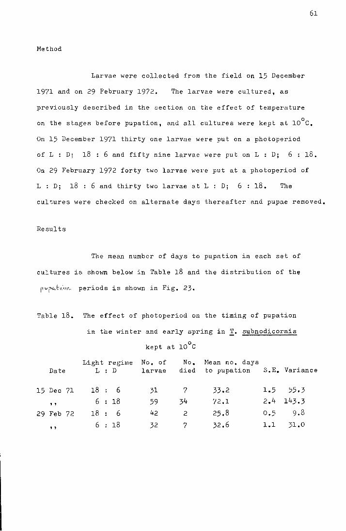
61

Method

Larvae were collected from the field on 15 December

1971 and on 29 February 1972. The larvae were cultured, as

previously described in the section on the effect of temperature

0 on the stages before pupation, and all cultures were kept at 10 C.

On 15 December 1971 thirty one larvae were put on a photoperiod

of L : D; 18 : 6 and fifty nine larvae were put on L : D; 6 : 18.

On 29 February 1972 forty two larvae were put at a photoperiod of

L : D; 18 : 6 and thirty two larvae at L : D; 6 : 18. The

cultures were checked on alternate days thereafter and pupae removed.

Results

The mean number of days to pupation in each set of

cultures is sho\m below in Table 18 and the distribution of the

f"pc...tr·o,t... periods is shown in Fig. 23.

Ta.ble 18. The effect of photoperiod on the timing of pupation

in the winter and early spring in T. subnodicornis

kept at l0°C

Light regime No. of No. Nean no. days Date L D larvae died to pupation s.E. Variance

15 Dec 71 18 6 31 7 33.2 1.5 55.3

' ' 6 18 59 34 72.1 2.4 143.3

29 Feb 72 18 6 42 2 25.8 0.5 9.8

' ' 6 18 32 7 32.6 1.1 31.0

Fig. 23. The distribution of dates of pupation for

!· subnodicornis on long (L:D; 18:6) and

short (L:D; 6:18) photoperiods. Upper

histogram shows pupation dates of cultures

set up on 15 December 1971 and lower histogram

shows pupation dates of cultures set up on

29 February 1972.

D L:D; 18:6

rzi L:D; 6:18

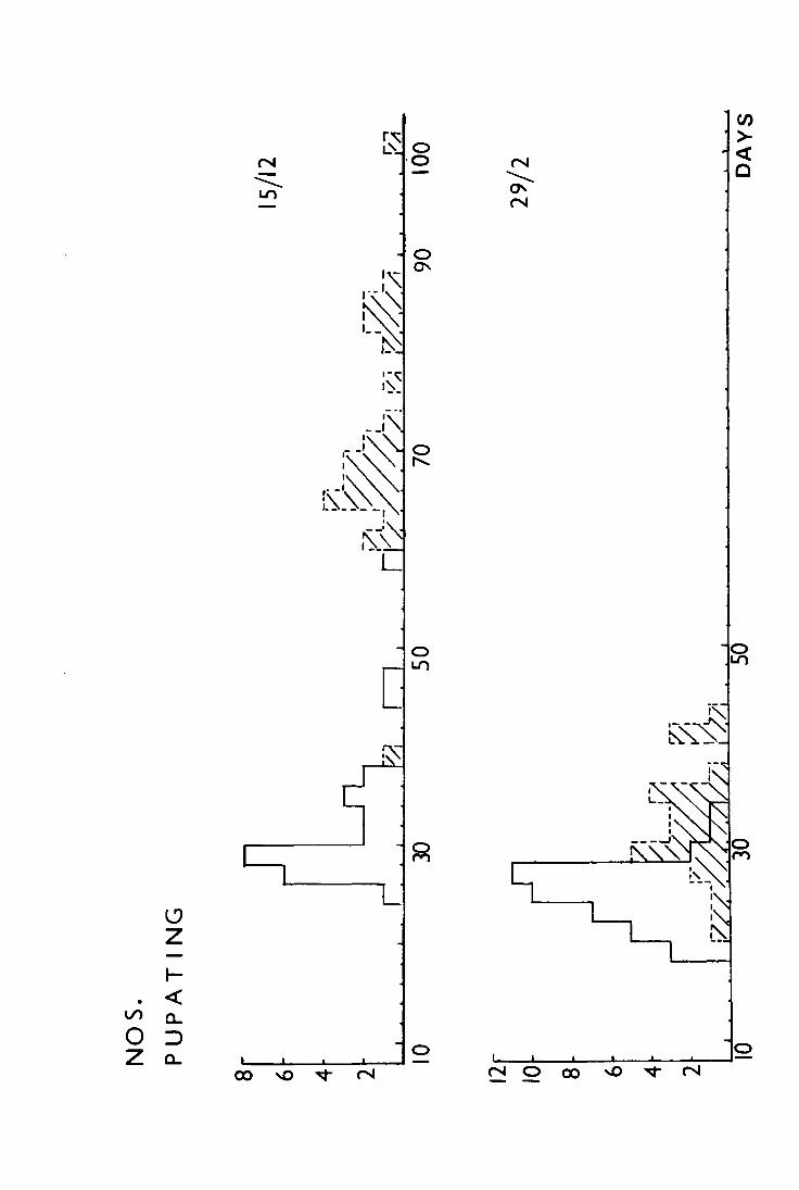
l? z ...... <

Vl CL

0 :::> z CL

CX) '-'>

0

v N 00 ..0 v N

CJ)

> <t 0

0

62

Before Christmas short photoperiod had a marked effect

in retarding pupation even when the larvae were kept at, what

would be in the field, high spring temperatures. By 29 February

1972 the photoperiod effect was much smaller. The means of the

number of days to pupation on the two light regimes, although

significantly different (t = 5.6, P<:::O.OOl), were only seven

days apart, and the variance for the short day regime, although

significantly different from that of the long day regime

(F = 3.2, p < 0.01) had decreased considerably.

It appears from these results that fourth instar

!· subnodicornis larvae develop slowly towards pupation at

10°C on a short day photoperiod. This process is accelerated

and pupation synchronised by a long day regime. This would

have considerable adaptive significance in the field, making

it possible for larvae to maintain an annual cycle by restra.ining

larvae from pupating during a warm "linter and synchronising

the emergence period. The mechanism of the photoperiod

effect will be discussed later when the reaction of an autumn

emerging tipulid, !• pagana Meigen has been described.

2. The effect of photoperiod on the termination of diapause

in T. pagana

In addition to looking at the photoperiod reaction

in T. subnodicornis an autumn emerging species, !• pagana,

was studied for comparison. !· pagana lays its eggs, \,rhich

hatch throughout the winter and early spring, in October at

1>1oor House. Growth is very rapid until late June when the

. l

larvae cease to eat and become relatively inactive. Pupation

takes place in September. In the period betHeen June and

September the metabolic rate drops and unlike the over-wintering

stage in !· subnodicornis, in Hhich feeding and activity continue,

the larvae are considered to be undergoing a true diapause in the

sense of Harvey (1962).

In 1971 a preliminary experiment indicated that the

diapause in !· pagana was broken by a short (L : D; 6 : 18)

as opposed to a long (L : D; 18 6) photoperiod and that

pupation was not triggered by drop in temperature as suggested

by Horobin (1971). In 1972 a further experiment designed to

find the critical photoperiod was set up.

Method

Cultures of !· pagana larvae were set up on 10 July

1972 when the larvae were already in their passive state.

The culture method used was similar to that for fourth instar

larvae of T. subnodicornis with the exception that the mosses

from which the larvae were collected were substituted for

liverworts. T t t th . t 1 t at 15°C wen y o 1r y arvae were pu on

the following light regimes L : D; 18 : 6, L : D; 16 8,

L : D; 14 : 10, and L : D; 12 : 12.

Results

The number of days until the mean emergence date

on each regime is shown in Table 19 and the distribution of

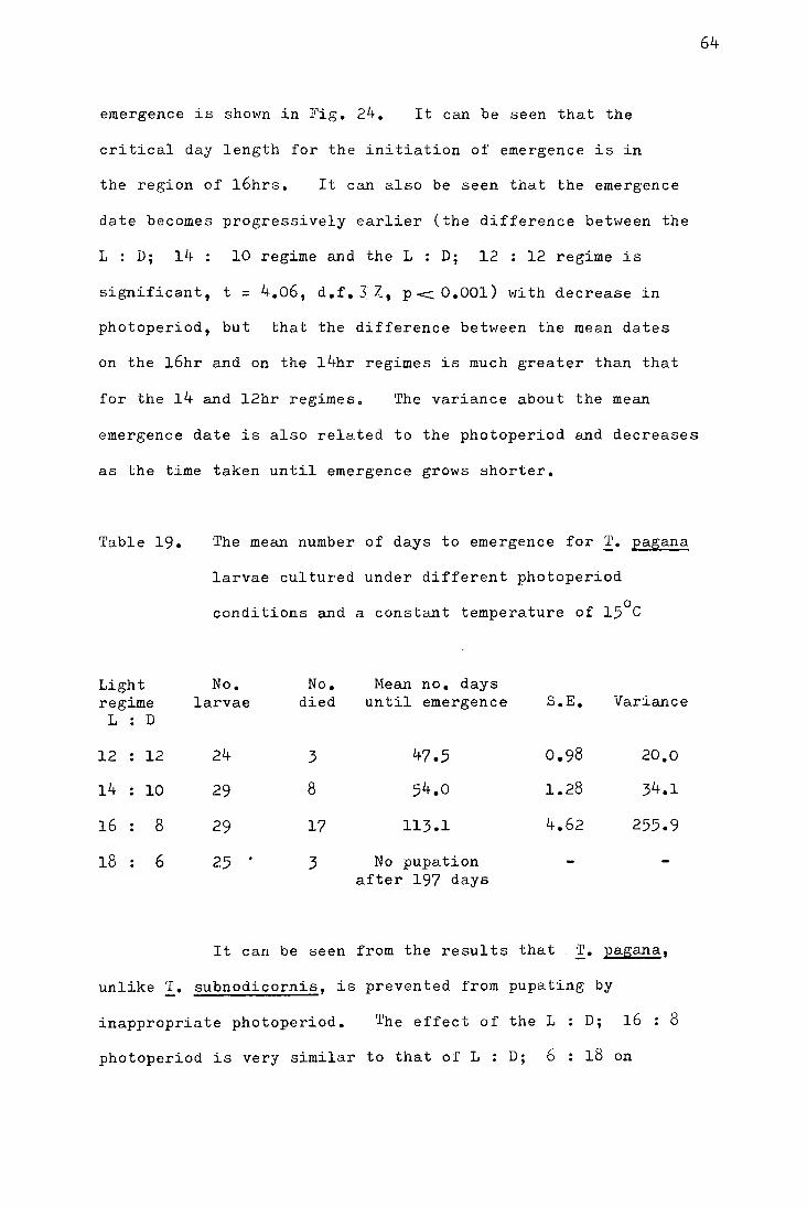
emergence is shown in Fig. 24. It can be seen that the

critical day length for the initiation of emergence is in

the region of 16hrs. It can also be seen that the emergence

date becomes progressively earlier (the difference between the

L : D; 14 : 10 regime and the L : D; 12 : 12 regime is

significant, t = 4.06, d.f. 3_ 1., P< 0.001) with decrease in

photoperiod, but that the difference between the mean dates

on the 16hr and on the 14hr regimes is much greater than that

for the 14 and 12hr regimes. The variance about the mean

emergence date is also related to the photoperiod and decreases

as the time taken until emergence grows shorter.

Table 19.

Light regime

L D

12 12

14 10

16 8

18 6

The mean number of days to emergence for !· pagana

larvae cultured under different photoperiod

conditions and a constant temperature of 15°C

No. No. 1'1ean no. days larvae died until emergence S.E. Variance

24 3 47.5 0.98 20.0

29 8 54.0 1.28 34.1

29 17 113.1 4.62 255.9

25 3 No pupation after 197 days

It can be seen from the results that . !· pagana,

unlike T. subnodicornis, is prevented from pupating by

inappropriate photoperiod. The effect of the L D; 16 8

photoperiod is very similar to that of L : D; 6 18 on

64

Fig. 24. Distribution of emergence dates for !· pagana

inJ:aooratory-ouTtures set-up-at "1"5°0 and-at--­

three different photoperiods on 10 July 1972.

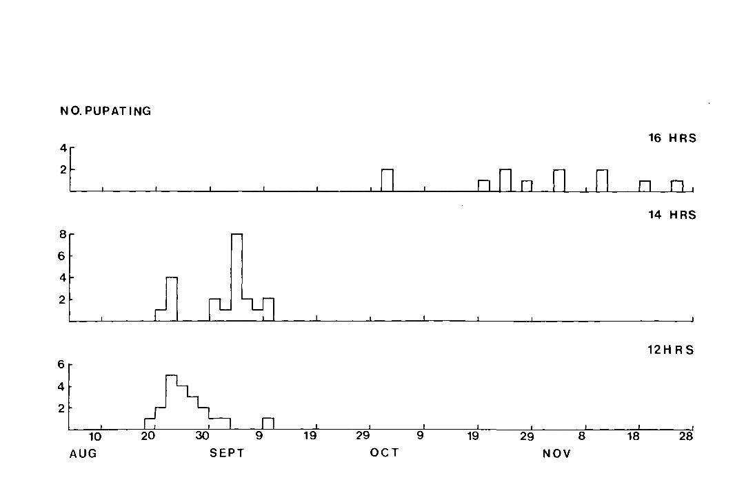
NO. PUPATING

4f 16 HAS

2

I I I I I ~D I nOn 0 .0 o o.

8

6

4

2

6

4

2

10

AUG SEPT 29 9 19

OCT

14 HRS

12H RS

29 8 18 28

NOV

~. subnodicornis in that the synchrony of emergence has been

lost. It is clear from the decrease in variance with the

decreased photoperiod that the shortening day length will

have the effect, not only of breaking diapause, but of

synchronising the emergence in the field. The effect that

decreasing photoperiod between 14 and l2hrs has on advancing

the mean emergence date will have adaptive significance in

the field by promoting the emergence of flies that have been

slow in breaking diapause.

3. Discussion

Beck (1968) remarks that "the importance of

photoperiodism in the seasonal development and ecological

adaptations of univoltine species is little appreciated

and has been investigated in very few forms". Considerable

work has been carried out on the initiation and termination

of diapause, especially in the Lepidoptera (Danilevskii 1965)

in multivoltine species. Diapause is defined as a period

when development is "spontaneously11 arrested ( Shelford 1929)

in contrast to the situation when unfavourable conditions

impose restrictions on the metabolism. The diapause state

is characterised by a decrease in activity and a drop in

metabolic rate and may occur automatically as a stage in the

life-history, as in the egg stage of the grasshopper

Austroicetes cruciata Sauss. (Andrewartha l943b), or it may

be triggered by some aspect of the environment, such as a

specific day length. Either summer or winter can constitute

an unfavourable period, but it is more usual for polycyclic

65

I

r ,'f ~

66

insects in temperate climates to have their growth period

during the warmer part of the year and to react to short

day length by going into diapause. In this way the least

vulnerable stage is subjected to the winter temperature and

any problem of food shortage is avoided.

In a univoltine insect such as !· pagana the

reaction to photoperiod performs two functions. Short day

length both breaks diapause and synchronises emergence.

Probably the main function of diapause in this case is that

it is broken by a precisely timed signal which synchronises

emergence. It has not been demonstrated but it is probable

that larvae do not enter diapause until they are fully grown

and that under an 18hr day they diapause, according to the

temperature they have experienced in the field, over a

considerable time period; alternatively, they may enter

diapause a fixed number of days after the final larval moult

as does Phyllopertha hortiola (Laughlin 1963). In T. subnodicornis

the photoperiod reaction is less familiar in that the larvae are

not technically diapausing through the winter (the reasons for

supposing !• pagana to be in diapause and !• subnodicornis not

will be discussed in the next section on respiration). Hov1ever,

the synchronising function of photoperiod is very similar to the

situation in T. pagana. It is interesting to note that

!• subnodicornis reacts to long day length and ~· pagana

to short day length. As the two species are in the same

genus it is likely that the physiological response is similar

in the two cases and that the photoperiod responded to is a

product of the selection pressure of the life-history and the

environment. Danilevskii ( 1965) has shown that even v1i thin one

species (Acronycta rumicis L.) the critical day length for diapause

initiation can change from 15 to 20hrs over a latitude range of 43° to 55°N.

IX Preliminary model for the life-cycle of !· subnodicornis

In most univoltine insects that have been studied

(Danilevskii 1965, Beck 1968) the yearly cycle which takes

place over a wide geographical range involving exposure to

widely different temperature regimes is made possible by a

diapause, defined as a stage in the life-history when there

is a "spontaneous" drop in the metabolic rate (:..;helford 1929).

In !· subnodicornis adaptations to both temperature and

photoperiod ensure a yearly life-cycle without the intervention

of diapause. The lengthening photoperiod in spring also has

the effect of synchronising the emergence period and this

second attribute is not an aspect that has been investigated

extensively.

Development of the egg, early instars and pupae

of T. subnodicornis respondSto an increase in temperature

over a comparatively wide range of temperature. In the

third and fourth instars the optimum temperature for

development drops and the increase in rate in response to rise

in temperature over the favourable temperature range decreases.

There may also be a response to shortening day length such

that larvae which are still growing increase their growth

rate (see p. 55 ) • These adaptations allow larvae developing

in the field, under a range of temperature conditions, to

finish their growth period before the onset of winter.

It is suggested that the completion of growth

is followed by a period which is either temperature independent

or proceeds more quickly at lower temperatures. The onset of

this phase prevents larvae from warm areas progressing towards

67

pupation before Christmas. ~his stage takes place under a

period of short day length and can be broken by putting the

larvae onto a long photoperiod. In the field larvae would

enter this phase between early November and January. By

the beginning of March the day length of lOhrs no longer

inhibits temperature dependent development and larvae can

progress to pupation. 'I'he mean pupation date, and, in

consequence, the mean emergence date will be directly

related to the temperature from March onwards. Fig. 25

shows the duration of different stages of the life-history

under a range of temperature conditions and long and short

day length in the laboratory.

68

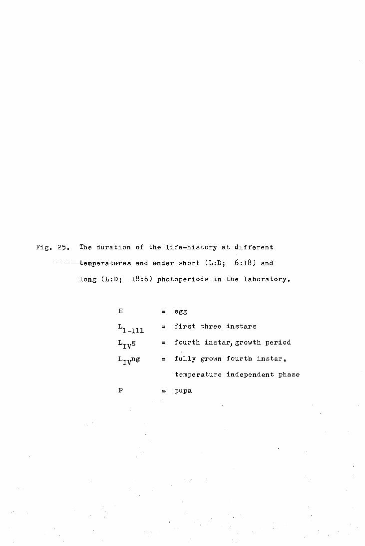
Fig. 25. The duration of the life-history at different

---tempera-tu-res and unde-I' short (-L-:-D; -6-:18)-and

long (L:D; 18:6) photoperiods in the laboratory.

E_ = egg

Ll-lll = first three in stars

LIVg = fourth instarJgrowth period

Liyng = fully grown fourth instar,

temperature independent phase

p = pupa

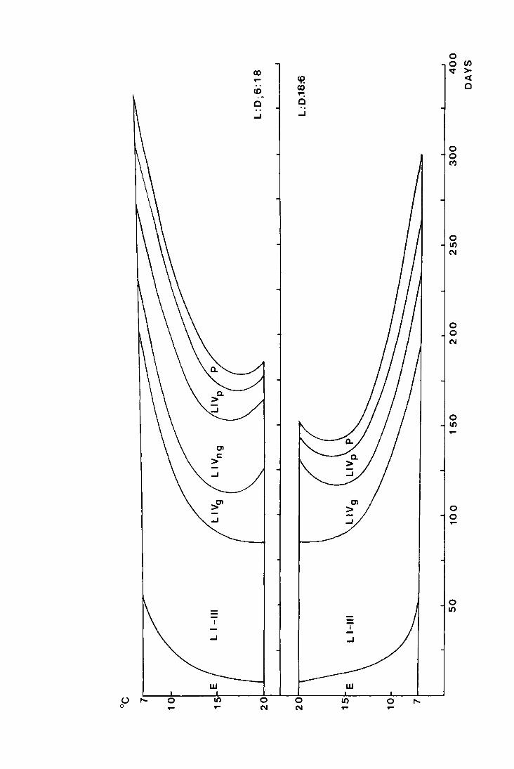
u ,... 0 ,....

LIJ

,....

co ,.... <D . -c

0 ('II

~ co ...-:, c .. ...J

0 ('II

LIJ

10 0 ,.... ,....

0 0 v

0 0 (")

0 10 ('II

0 0 ('II

0 10 ,....

0 0 ,....

0 10

en > <(

c

X. RESPIRATION RATES IN THE LARVAL STAGES OF

T. SUBNODICORNIS f~D !• PAGANA

Introduction

The respiration rates were measured to give a

comparative indication of the metabolic rate under different

conditions. In the case of T. subnodicornis it was thought

that a possible explanation for the growth rates being so

similar under widely different temperature conditions in the

field v:as that the larvae were acclimatised to the temperature

at which they were developing. This theory was tested by

bringing larvae into the laboratory, keeping them on different

temperature regimes for about three weeks, and then comparing

the respiration rates.

As it was thought that the stage before pupation

in T. pagana constituted a true diapause, the respiration

rates of larvae in July were compared with those of over-

wintering !· subnodicornis larvae. A further experiment

was made to see whether there was a difference in the

respiration rates of T. pagana larvae on a long day,

diapause inducing photoperiod, and a short day, pupation

initiating photoperiod.

Measurement of respiration rate

Respiration rates were measured in Warburg

manometers filled with Brodies' fluid (Dixon 1951).

lOml reaction flasks vJere used and kept at constant

70

temperature by immersion in a thermostatically controlled

water bath. Each larva was weighed and placed, unrestrained,

in a reaction flask. O.lml of 2N potassium hydroxide was

added to the central well to absorb carbon dioxide and 0.2ml

of distilled water was put in the flask to keep the larva

damp. The respiration rates were measured over periods of

6 - lOhrs for each larva.

la. Method - T. subnodicornis

All measurements were carried out between the end

of October and mid December. The acclimatisation temperatures

d 15° d 5°C and all th 0 t 0 t use were an e resp1ra 1on ra es were

measured at l5°C. Larvae were brought in from the field

in early December and kept at the appropriate acclimatisation

temperature until testing. Their respiration rates were

compared with those of larvae taken straight from the field

in late October and with those of larvae that had been reared

at 15° and 5°C in the laboratory. Hearing and acclimatisation

were carried out under an L : D; 18 : 6 photoperiod regime

and the rate of respiration was measured during the photophase.

lb. Results

The respiration rates of each group of larvae

are shown below in Table 20. 'l'he mean respiration rates

of individual larvae are shown in Table X in the appendix.

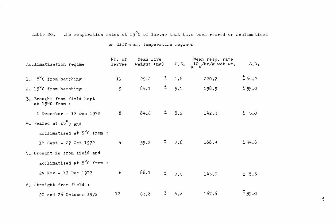
Table 20. The respiration rates at 15°C of larvae that have been reared or acclimatised

on different temperature regimes

No. of Hean live Mean resp. rate Acclimatisation regime larvae weight (mg) S.E. ~102/hr/g wet wt. S.D.

5°C from hatching + 1.8 +

1. 11 29.2 - 220.7 - 64.2

2. 15°C from hatching 9 84.1 + 5.1 138.3 ~ 35.0 -

3. Brought from field kept at 15°C from

1 December - 17 Dec 1972 8 84.6 + 8.2 142.3 + 5.0 - -0

4. Reared at 15 C and

acclimatised at 5°C from

16 Sept - 27 Oct 1972 4 55.2 + 7.6 188.9 ! 34.6 -

5. Brought in from field and

acclimatised at 5°C from

24 Nov - 17 Dec 1972 6 86.1 + 7.0 143.3 + 5.3 - -6. Straight from field

+ + 20 and 26 October 1972 12 63.8 - 4.6 167.6 -35.0

-.,_)

f-'

There is a significant difference between the

0 respiration rates of the larvae reared at 5 C (group 1) and

0 those reared at 15 C (group 2) (t = 3.6, d. f. 16, p ~ QOl),

but it is more likely that this is an effect of size difference

(Bertalanffy 1957) rather than due to acclimatisation to two

different temperature regimes. (When the regression of

respiration rate per hour per g wet weight (y) against wet

weight in mg (x) for the twenty one larvae that had been

reared or acclimatised at 5°C was made, the following

equation was obtained : y = 242.4- 0.989x. On the basis

of this regression the respiration rates for larvae with

mean weights of 29.2mgand 84.lmg should be 213.5 and 159.3~1

of o2

per g perh respectively, neither of which are

significantly different from the actual figures recorded.)

The difference between the two groups brought in

from the field (groups 3 and 5 , where the weights are

comparable)and acclimatised at 5° and 15°C respectively,

is not significant; and if the two groups that have been

acclimatised at 5°C (4 and 5) are compared with those that

have been reared and acclimatised at 15°C (2 and 3), the

rate is still not significantly different (t = 1.85, p:> 0.05).

lc. Conclusion

When invertebrates are wholly or partly acclimatised

to low temperature they often display a higher initial

respiration rate when they are moved to a higher temperature

than animals that have been kept at this temperature

(Bullock 1955). However, Scholander et al. (1953) found

72

73

no evidence of this type of reaction in tropical and arctic

insects and from the data above it seems unlikely that

T. subnodicornis shows acclimatisation. In the case of

T. subnodicornis, however, the larvae were not restrained

during tests and it is possible that their activity masked

the small differences in respiration rates due to the differences

in basal metabolic rates. lmother criticism is that most of

the tests were carried out when the larvae had finished growth.

If immobilized larvae were used, and their respiration rates

throughout the year were measured, it might be found that

acclimatisation occurred during the growth period. However,

from the experimental data on grO\·Ith and the timing of the

stages in the life-history, there is no necessity to invoke

acclimatisation to explain the synchrony of development.

It can be seen from the comparison of the larvae

in the various weight ranges that diapause does not occur.

The drop in respiration rate per g wet weight shown by the

older larvae can be accounted for in terms of increased

weight alone.

2a. Method - !· pagana

T. pagana larvae were taken from the field on

16 July 1972 and divided into two groups which were cultured

as previously described (p. 63). Both groups were kept at

0 15 C and one set of cultures wa.s placed on a photoperiod

regime of L : D; 18 : 6, while the other was put on an

L : D; 10 :14 regime. The respiration rates of larvae

from both groups were measured on 27 July 1972 during the

photophase of both light regimes.

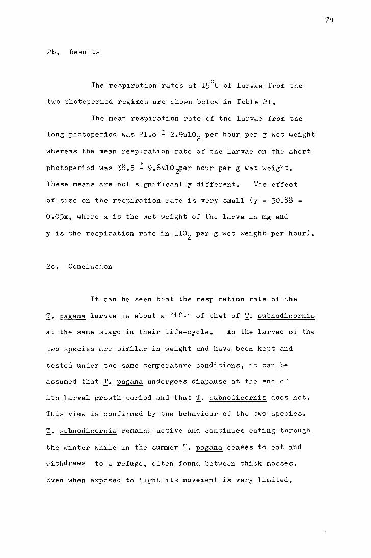
2b. Results

The respiration rates at l5°C of larvae from the

two photoperiod regimes are shown below in Table 21.

The mean respiration rate of the larvae from the

long photoperiod was 21.8 ! 2.9~102 per hour per g wet weight

whereas the mean respiration rate of the larvae on the short

photoperiod was 38.5 ~ 9.6~0~er hour per g wet weight.

These means are not significantly different. 'Ehe effect

of size on the respiration rate is very small (y = 30.88 -

0.05x, where X is the wet \•Ieight of the larva in mg and

y is the respiration rate in ~10 2 per g wet weight per hour).

2c. Conclusion

It can be seen that the respiration rate of the

T. pagana larvae is about a fifth of that of T. subnodicornis

at the same stage in their life-cycle. As the larvae of the

two species are similar in weight and have been kept and

tested under the same temperature conditions, it can be

assumed that !• pagana undergoes diapause at the end of

its larval growth period and that !· subnodicornis does not.

This view is confirmed by the behaviour of the two species.

T. subnodicornis remains active and continues eating through

the winter while in the summer !· pagana ceases to eat and

vii thdraws to a refuge, oi'ten found between thick mosses.

Even when exposed to light its movement is very limited.

74

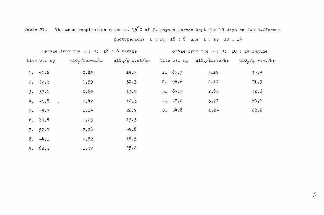
Table 21. The mean respiration rates at 15°C of _!. pagana larvae kept for 10 days on two different

photoperiods L : D; 18 : 6 and L : D; 10 : 14

Larvae from the L : D; 18 : 6 regime Larvae from the L : D; 10 : 14 regime

Live Ht. mg ).l102/1arva/hr ).1.102/g w.wt/hr Live wt. mg ).l102/1arva/hr ).1.10~/g w.wt/hr c:.

1. 41.6 o.82 19.7 1. 87.3 3.15 35.9

2. 52.3 1.59 30.3 2. 98.6 2.10 21.3

3. 57.1 o.8o 13.9 3. 87.3 2.85 32.6

4. 45.8 0.47 10.3 4. 47 .o 3.77 80.2

5. 49.7 1.14 22.9 5. 54.8 1.24 22.2

6. 80.8 1.23 15.3

7. 57.2 2.28 39.8

8. 44.1 o.82 18.5

9. 62.5 1.57 25.2

--:! \J1

If !· pagana undergoes diapause it would be

expected that the respiration rate would rise when diapause

is terminated and progress towards pupation begins (Endelman

1951 in Lees 1955). 1hat this has not been recorded in

!· pagana may be due to the measurements being carried out

before diapause had been broken. The larvae pupated between

28 July and 5 August 1972 and it is possible that larva no.4

is the only larva in the group from the short photoperiod

that had ended diapause. Further information on this and

the growth stages of the life-cycle is. needed.

76

XI !'10RTALI'l'Y RATE THRC!UGHOUT THE LIFE-HISTORY OF

'l'. SUBNODICORNIS

Information on mortality rate at different stages

in the life-history of T. subnodicornis has been gained from

observations in the field and labora_tory. As explained below,

the number of samples that could be sorted was limited so the

population study in the field has been concentrated on the

fourth instar and adults. Coulson (1962) showed the pattern

of mortality throughout the life-history on one site. In this

study several sites have been compared.

la. Sampling method for larvae

An approximation to stratified random sampling was

made by dividing each site into eight equal areas and srunpling

from each area. A corer of 1.9cm radius was used to sample

for eggs and first instar larvae and a corer of 5.7cm radius

was used for the later stages.

Throughout the study the size and number of cores

taken were related to the number of srunples that could be

sorted in the time available. Coulson (1962) used a flotation

method in which cores were macerated in magnesium sulphate

solution (sp.gr.l.23) to extract first instars and eggs.

In this study, where the densities were lower and a number

of sites were being compared, the method was found to be too

time-consuming to process enough samples to give useful

figures on egg density and hatching success. An attempt to

adapt the wet funnel regimes, used by Hadley (1966) and Horobin

77

(1971) for extracting Molophilus ater, also proved unsuccessful,

so first instar estimations were made on only a few occasions.

It was found that during heat extraction for the

later instars in Berlese funnels almost as many larvae died

within the core as were extracted, so hand sorting was used.

This was found to be an efficient method for fourth instar

larvae. In the autumn of 1970 forty cores, radius 5.7cm,

were hand sorted and 34 larvae removed. Further careful

sieving and washing yielded only one further larva which was

dead. Subsequent checks by double sorting samples indicated

that this level of efficiency was maintained.

Coulson (1962) found that, at the densities at which

he was studying them, larvae showed no significant tendency

to aggregate, so he used the mean as the best estimate of

the variance. During this study a high density site on

Knock Fell was found in spring 1972 and sampling beb-teen

28 February 1972 anili 24 March 1972 confirmed that in the

spring fourth instar larvae are distributed randomly.

The comparison of the data with those for the equivalent

Poisson distribution is shown in Table 22.

Further tests on distrj_butions at lower densities

also failed to show significant deviation from the appropriate

Poisson distribution. 60 cores taken from blanket-bog in

autumn 1970 with a mean of 0.567 larvae per core gave a X 2

valu~ of 0.28, d.f. 2, p;> 0.1 and 165 cores (0.436 larvae

per core) from a set of Juncus sites chosen as having a

2 density of approximately 40 larvae/m gave a value of 2.06,

d.f. 2, p_;:::.O.l.

78

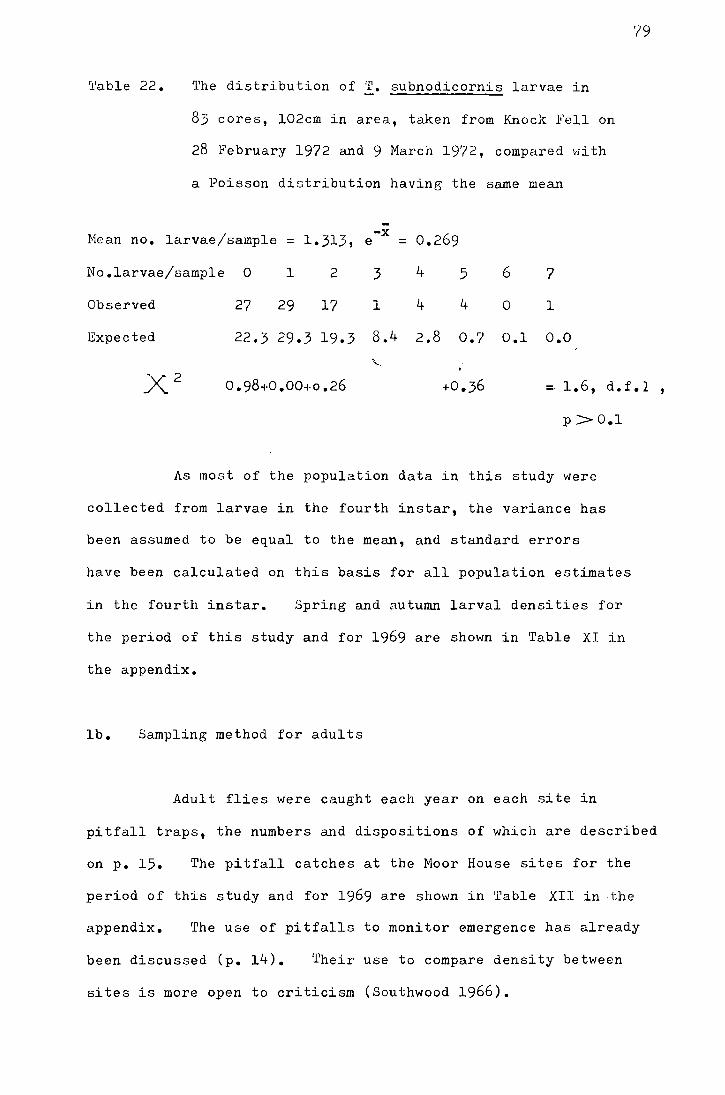
'l'able 22. The distribution of !· subnodicornis larvae in

83 cores, l02cm in area, taken from Knock Fell on

28 February 1972 and 9 March 1972, compared vJith

a Poisson distribution havine the same mean

Nean no. larvae/sample =

No.larvae/sample 0 l

Observed 27 29

1.313,

2

17

-x e

3

l

8.4

= 0.269

4 5

4 4

2.8 0.7

6

0

0.1

7

l

o.o Expected 22.3 29.3 19.3

79

=- 1.6, d.f.2

p>O.l

As most of the population data in this study were

collected from larvae in the fourth instar, the variance has

been assumed to be equal to the mean, and standard errors

have been calculated on this basis for all population estimates

in the fourth instar. Spring and autumn larval densities for

the period of this study and for 1969 are shown in Table XI in

the appendix.

lb. Sampling method for adults

Adult flies were caught each year on each site in

pitfall traps, the numbers and dispositions of which are described

on p. 15. The pitfall catches at the Moor House sites for the

period of this study and for 1969 are shown in Table XII in the

appendix. The use of pitfalls to monitor emergence has already

been discussed (p. 14). Their use to compare density between

sites is more open to criticism (Southwood 1966).

The difference in activity level at sites of different altitude

was appreciable in that it was very rare to see males flying

above 2500ft and it is possible that the activity of the

females too was curtailed on the colder sites. In addition,

Greenslade (1964) demonstrated that for carabids the pitfall

catch is influenced by the surrounding vegetation. This is

relevant to this study in which the two main vegetation types,

blanket-bog and Juncus or Eriophorum sward have such different

growth characteristics.

The value of using the pitfall catch as a comparative

density measurement has been examined by comparing the pitfall

catches with the spring larval densities which should represent

the maximum possible number of adults/m2

on each site. The

sites used are those on the east side and therefore at approx-

imately the same altitude, but as it was thought likely that

female catch was less affected by weather than the male catch,

correlations have been carried out for both the total catch

So

and the female pitfall catch. In the first pair of correlations

all sites, except the Behind House site in 1972 which was flooded

during most of the emergence period, have been included. In the

second pair the blanket-bog sites and the Behind House site in

1972 have been omitted, and in the third pair the 1969 results

have been left out as well. During 1969 numbers of flies

varying betlveen 1307 and 2881 (6/m2

and l3/m2

respectively)

were removed from each site, and as this constituted a large

part of the calculated population, the pitfall catch must have

been diminished as a consequence. The results of these

correlations and the regression parameters, derived at the 0ame

time for adult pitfall catch and spring larval density, are

shown in 'l'able 23.

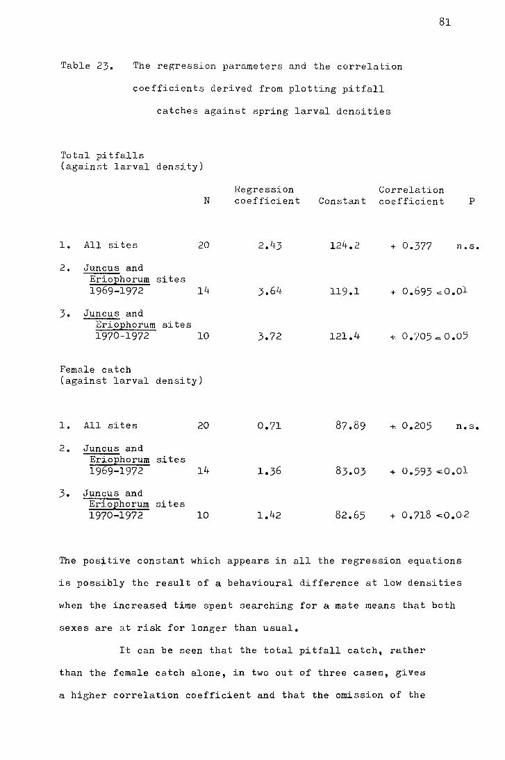
81

Table 23. The regression parameters and the correlation

coefficients derived from plotting pitfall

catches against spring larval densities

Total pitfalls (against larval density)

N !~egression

coefficient Correlation

Constant coefficient p

l. All sites 20 2.43 124.2 + 0.377 n.s.

2. Juncus and ErioEhorum sites 1969-1972 14 3.64 119.1 + o.695.:.o.ol

3. Juncus and ErioEhorum sites 1970-1972 10 3.72 121.4 + 0.705.c::0.05

Female catch (against larval density)

l. All sites 20 0.71 87.89 +. 0.205 n.s.

2. Juncus and ErioEhorum sites 1969-1972 14 1.36 83.03 + 0.593 c:.0.01

3. Juncus and ErioEhorum sites 1970-1972 10 1.42 82.65 + 0.718 <0.0·2

The positive constant which appears in all the regression equations

is possibly the result of a behavioural difference at low densities

when the increased time spent searching for a mate means that both

sexes are at risk for longer than usual.

It can be seen that the total pitfall catch, rather

than the female catch alone, in two out of three cases, gives

a higher correlation coefficient and that the omission of the

Fig. 26. The regression of pitfall catch on Juncus areas

on spring larval density from 1969 - 1972. The

blanket-bog densities are also shown but not

included in the regression.

y = 3.72x + 121.4, r = +0.705, p~ OPl

• 1969 Juncus sites

o Blanket bog

o 1970, 1971 and 1972 Juncus sites

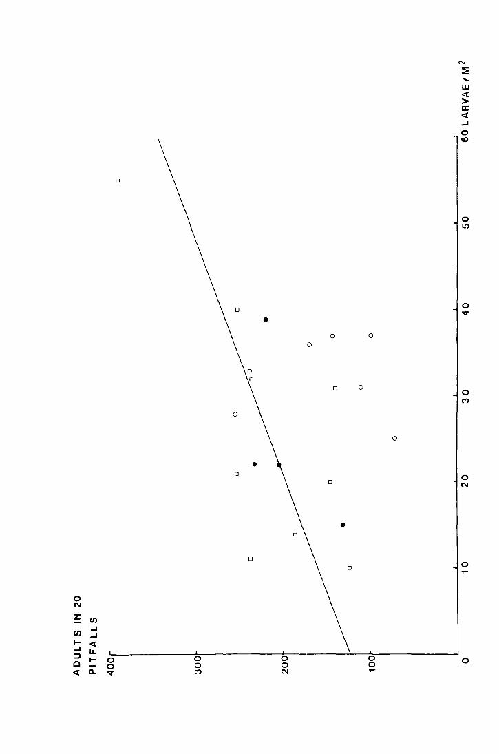
0

0 0 0

0 0

!J

0

~ ..... w <(

> a: <(

..J

0 ID

0 II)

0 "'="

0 (")

0 N

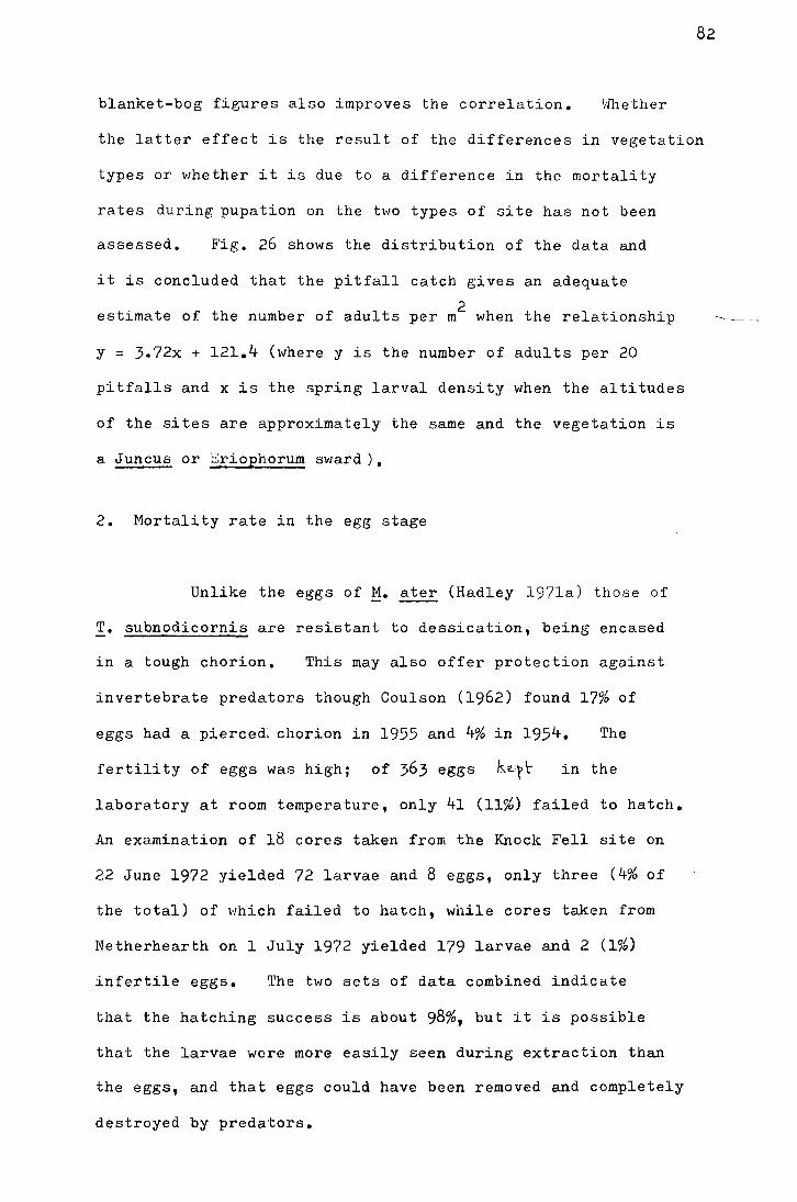
82

blanket-bog figures also improves the correlation. Hhether

the latter effect is the result of the differences in vegetation

types or whether it is due to a difference in the mortality

rates during pupation on the two types of site has not been

assessed. F'ig. 26 shows the distribution of the data and

it is concluded that the pitfall catch gives an adequate

2 estimate of the number of adults per m when the relationship

y = 3.72x + 121.4 (where y is the number of adults per 20

pitfalls and x is the spring larval density when the altitudes

of the sites are approximately the same and the vegetation is

a Juncus or Eriophorum sward).

2. Mortality rate in the egg stage

Unlike the eggs of ~· ater (Hadley 197la) those of

T. subnodicornis are resistant to dessication, being encased

in a tough chorion. This may also offer protection against

invertebrate predators though Coulson (1962) found 17% of

eggs had a pierced. chorion in 1955 and 4% in 1954. The

fertility of eggs was high; of 363 eggs k~r~ in the

laboratory at room temperature, only 41 (11%) failed to hatch.

An examination of 18 cores taken from the Knock F'ell site on

22 June 1972 yielded 72 larvae and 8 eggs, only three (4% of

the total) of Hhich failed to hatch, while cores taken from

Netherhearth on 1 July 1972 yielded 179 larvae and 2 (1%)

infertile eggs. The two sets of data combined indicate

that the hatching success is about 98%, but it is possible

that the larvae were more easily seen during extraction than

the eggs, and that eggs could have been removed and completely

destroyed by predators.

---

3. Mortality rate in the first instar

Coulson (1962) showed that during the life-cycle

the heaviest mortality takes place during the first instar.

'l'his would be expected in an insect vJi th an annual life-history

producing a large number of eggs ( Deevey 1947). Coulson found

that between 28 June 1954 and 8 July 1954 there was an 82%

mortality (18,000 eggs/m2

to 3,300 larvae/ml. This type of

mortality rate was found on I~ock Fell in 1972. An estimated

2 2 13,750 eggs per m gave rise to 4,130 larvae/m , srunpled on

22 June 1972, a 70% mortality, and by 28 July 1972 the density

had dropped to 329 larvae per m2

, a 98% mortality. Coulson

(loc.cit.) considered that drought and the condition of the

ground are very important factors in the survival of the

early stages of T. subnodicornis and it is known that a wet

autumn promotes the survival of T. paludosa (Milne et al. 1965).

3a. The effect of experimental manipulation of density

on the first instar in the field

2 In 1971 ten 0.25m enclosures were set up at

Netherhearth before the beginning of emergence. Each

enclosure was formed by sinking four 20 x 50cm galvanised

strips into the ground to a depth of lOcm so as to form a

square. The corners were reinforced with "lawn edging"

and fine nylon net, hole diameter ln~, was placed over the

top and secured vJi th string. During the emergence period

the number of females emerging from each trap was supplemented '

with fertilised females from outside until traps 1 - 6 had

received ten each and traps 7 - 10 eighty each. On 4 July

1971 Lour cores (1.9cm radius) were taken from each trap and

sixteen were taken from the area surrounding the traps.

Results

2 The numbers of first instar larvae per m on 4 July

1971 within and without the enclosures are shown in Table 24.

2 The number of adult females per m has been calculated from

2 the spring larval density and the number of eggs per m has

been calculated from the regression y = 110.5x - 808, where

y =egg number andy= female wing length,made during 1969

(M. Sc. study). The mean wing length of the females on

Netherhearth in 1971 was 10.2mm so the mean fecundity was

considered to be 319 eggs per female.

The densities of larvae in the two sets of traps

have been tested, assuming that the number of larvae

extracted from each plot is proportional to the number of

females introduced. X 2 = 4.7, d.f. 1, P-<0.05 9 indicating

that this was not the case and that survival at the higher

density was less than expected. This result was corroborated

by the data from the area outside the enclosures where the

2 density of females was calculated to be approximately 6 per m •

·x2 0hen the three densities are tested together = 48.98,

d.f. 2, p...:::::::O.OOl. It was therefore considered that mortality

in the first instar is higher at higher densities.

84

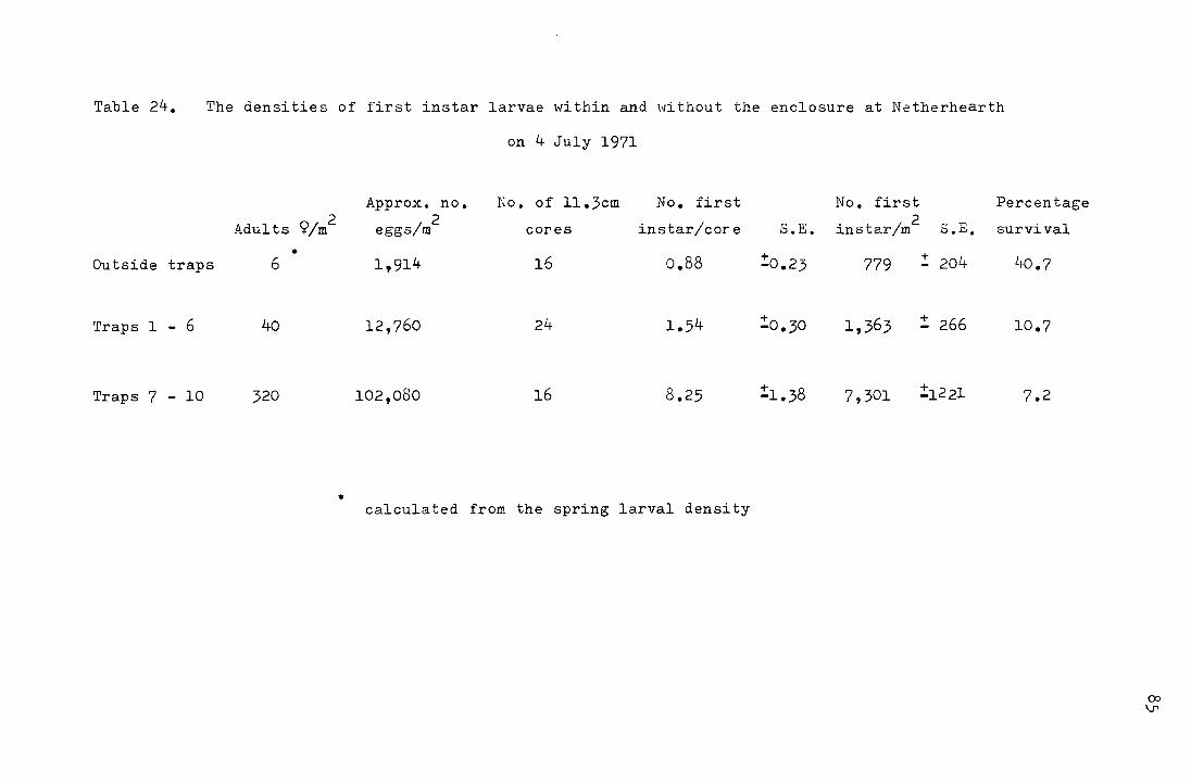
Table 24. The densities of first ins tar larvae within and \•li thou t the enclosure at Netherhearth

on 4 July 1971

Approx. no. No. of 11.3cm No. first No. first Percentage 2 2 instar/core instar/m2 Adults 9/m eggs/m cores S.E. s.E. survival

• + ! 204 Outside traps 6 1,914 16 o.88 -0.23 779 40.7

Traps 1 - 6 40 12,760 24 1.54 + -0.30 1,363 :!:. 266 10.7

Traps 7 - 10 320 102,080 16 8.25 :!:1.38 7,301 :!:.1221 7.2

• calculated from the spring larval density

<X> \Jl

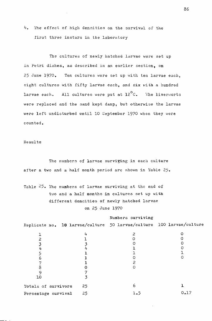
4. The effect of high densities on the survival of the

first three instars in the laboratory

The cultures of newly hatched larvae were set up

in Petri dishes, as described in an earlier section, on

25 June 1970. Ten cultures were set up with ten larvae each,

eight cultures with fifty larvae each, and six with a hundred

larvae each. 0

All cultures were put at 12 C. 'l'he li venrorts

were replaced and the sand kept damp, but otherwise the larvae

were left undisturbed until 10 September 1970 when they were

counted.

Results

The numbers of larvae survi~.ing in each culture

after a two and a half month period are shown in 'l'able 25.

Table 25. The numbers of larvae surviving at the end of

two and a half months in cultures set up with

different densities of newly hatched larvae

on 25 June 1970

Numbers surviving

86

Replicate no. 16 larvae/culture 50 larvae/culture 100 larvae/culture

l 4 2 0 2 l 0 0

3 3 0 0 4 4 l 0

5 l l l 6 l 0 0

7 l 2 8 0 0

9 7 10 3

Totals of survivors 25 6 l

Percentage survival 25 1.5 0.17

87

'll,·o x2 .w tests have been carried out, the first based

on the assumption that survival in the cultures should be in

proportion to the number of larvae introduced at the beginning

of the experiment, the second based on the assumption that

e~ch culture has a carrying capacity and that equal numbers

of larvae will survive per Petri dish at each density regime.

v-2 In the first case./'\.,. = 186.04, d.f. 2, p c::::O.OOl;. in the

V2 __ 8 second/'\. l .5, d.f. 2, p c:::.O.OOl. It appears that there

is a highly significant density-dependent effect and that

overcompensation occurs so that smaller numbers actually

survive at high densities. A further test was carried out

to test the significance of the differences between adjacent

pairs of density regimes, again based on the assumption that

there was no difference in the numbers surviving per Petri

dish. When the ten larvae per dish regime was compared with

I (x2__ ) the fifty larvae dish 7. 95, d. f. l, p < 0.01 , and when

the fifty larvae/dish regime was compared with the hundred

larvae/dish regime ()(2 = 2.33, d.f. 1, n.s.). The lack of

a significant difference between the last two figures can be

interpreted as that the overcrowding at fifty larvae per dish

has effects so drastic that they cannot readily be exceeded.

5. Mortality rate in the fourth instar

5a. Winter mortality in the field

The differences between the autumn and spring larval

densities shown in Table XI for each site have been tested using

Student's t-test. The percentage overwinter mortality at each site

in each year is shown in Table 26 and the level of significance

denoted.

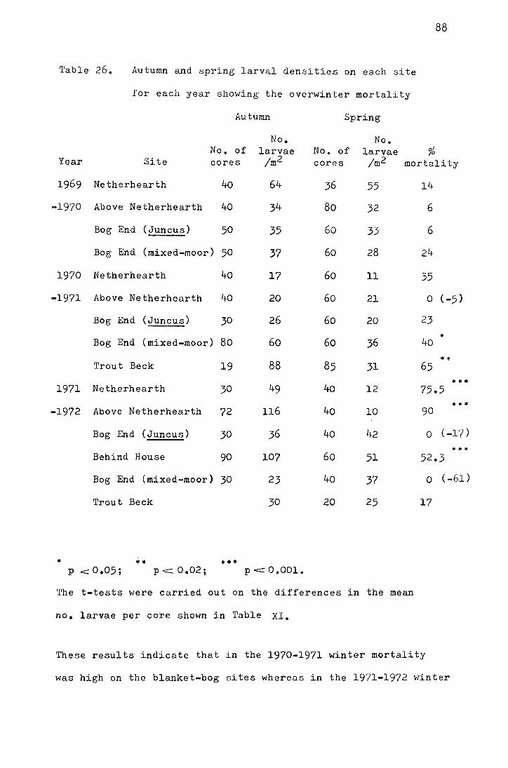
88

Table 26. Autumn and spring larval densities on each site

for each year showing the overwinter mortality

Autumn Spring

No. No. No. of larvae No. of larvae %

Year Site cores 1m2 cores 1m2 mortality

1969 Netherhearth 4o 64 36 55 14

-1970 Above Netherhearth 40 34 80 32 6

Bog End (Juncus) 50 35 60 33 6

Bog End (mixed-moor) 50 37 60 28 24

1970 Netherhearth 40 17 60 ll 35

-1971 Above Netherhearth 40 20 60 21 0 (-5)

Bog End (Juncus) 30 26 60 20 23

• Bog End (mixed-moor) 80 60 60 36 40

• * Trout Beck 19 88 85 31 65

••• 1971 Netherhearth 30 49 4o 12 75.5

••• -1972 Above Netherhearth 72 116 40 10 90

Bog End (Juncus) 30 36 40 42 0 ( -17)

••• Behind House 90 107 60 51 52.3

Bog End (mixed-moor) 30 23 40 37 0 (-61)

Trout Beck 30 20 25 17

• •• • •• p c:::::0.05; pc:::::::0.02; pc:::O.OOl.

The t-tests were carried out on the differences in the mean

no. larvae per core shown in Table XI.

These results indicate that in the 1970-1971 winter mortality

was high on the blanket-bog sites whereas in the 1971-1972 winter

mortality occurred largely on the Juncus sites and that none

of the sites suffered a significant decline in the 1969-1970

winter. ~here are not, however, sufficient data to be able

to attribute mortality to specific combinations of site and

weather conditions. It is interesting that significant

mortality occurs in the exceptionally mild winters of 1970-

1971 and 1971-1972, but not in 1969-70, but it is probably

not valid to make a direct comparison between the air

temperatures in each year as behJeen 1 November 1969 and

31 March 1970 there were seventy eight days of snow cover.

Oke and Hannel (1966) showed that a snow fall of 12.5cm

had such an insula~ing effect that although the snow surface

0 0 dropped to -17.3 c, the earth surface below remained at 0 C.

On a cleared area the soil showed a temperature gradient

from the surface to a depth of approximately 50cm. Oke and

Hannel give an example where, Hhen the air temperature was

-ll.3°C (a realistic minimum temperature for Moor House)

0 the temperature just below the surface was -7.2 C, at a

0 0 depth of 5cm it was -5 C, and at lOcm it was -3 C.

Fig. 27 shows the Moor House Grant recordings for

three thermistor probes in different positions on blanket-

bog for 5 January 1969 when snow was absent. It indicates

what a considerable buffering effect the vegetation and a

depth of lcm has on low temperatures. 0

-9 C was recorded

in the middle of an Eriophorum tussock, but at -lcm in

0 Juncus litter the temperature did not fall below -2 C.

It therefore seems possible that a short downward migration

Fig. 27. Grant recordings of hourly temperature readings

for thermistor probes in blanket-bog on 5 January 1969.

0 In Eriophorum tuesock

0 - 2om in Galluna .litter

- 2cm in Juncus litter

I I I

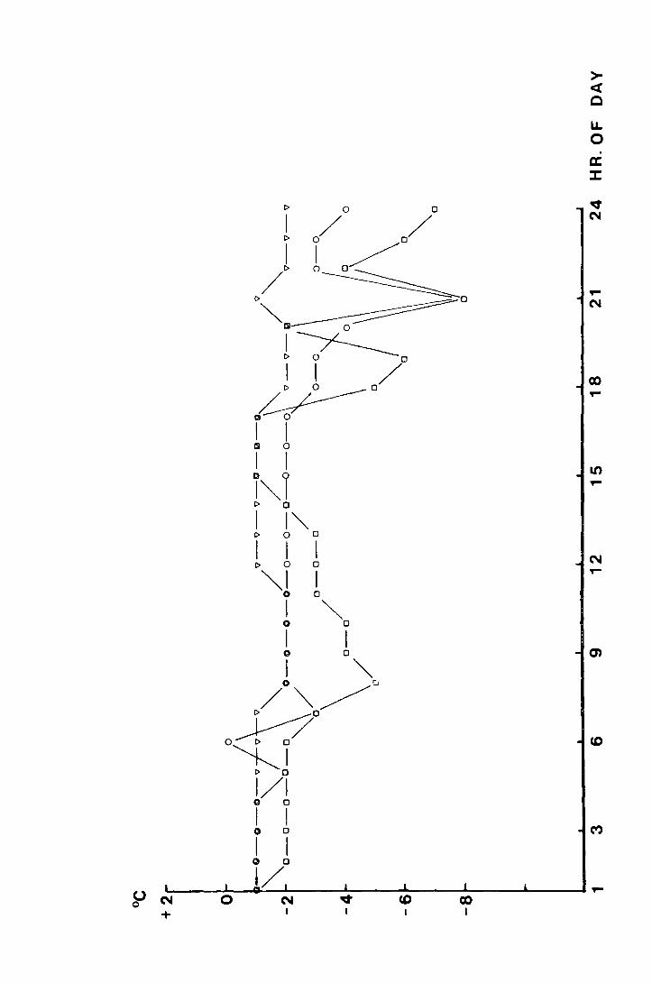
> <t 0

LL 0 . a: ::L

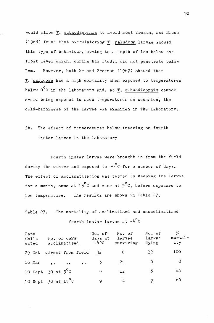
would allow T. subnodicornis to avoid most frosts, and Ricou

(1968) found that overwintering !· paludosa larvae showed

this type of behaviour, moving to a depth of lcm below the

frost level which, during his study, did not penetrate below

7cm. However, both he and Freeman (1967) showed that

!· paludosa had a high mortality when exposed to temperatures

0 below 0 C in the laboratory and, as T. subnodicornis cannot

avoid being exposed to such temperatures on occasion, the

cold-hardiness of the larvae was examined in the laboratory.

5b. The effect of temperatures below freezing on fourth

instar larvae in the laboratory

Fourth instar larvae were brought in from the field

0 during the winter and exposed to -4 C for a number of days.

The effect of acclimatisation was tested by keeping the larvae

0 0 for a month, some at 15 C and some at 5 C, before exposure to

low temperature. The results are shown in Table 27.

·rable 27. The mortality of acclimatised and unacclimatised

fourth in star larvae at -4°C

Date No. of No. of No. of %

90

Coll- No. of days days at larvae larvae mortal-ected acclimatised -4°C surviving dying ity

29 Oct direct from field 32 0 32 100

16 Mar ' ' ' ' ' ' 3 24 0 0

10 Sept 30 at 5°C 9 12 8 40

10 Sept 30 at 15°C 9 4 7 64

91

These results show that T. subnodicornis larvae are

0 resistant to temperatures below 0 C. The effect of acclimatis-

ation at 5°C for thirty days is better but is not significantly

0 x2 different from a 15 C regime ( = 0.78, d.f. 1, n.s.) but the

experiment should be repeated with larger numbers of larvae

and at a lower acclimatisation temperature. Horobin (1971)

showed that in the case of !· paludosa survival of larvae at

0 -4.0 C was considerably improved when larvae had been

acclimatised at 6.0°C and 2.0°C rather than at l5°or 10°C

and that some larvae could withstand lOhrs at -6.o0 c when

0 they had been cultured at 2.0 C for the previous week.

The Grant records show that, during the 1968-1969

and 1969-1970 winters (there is a break in the records in

February 1969 but they are otherwise continuous), the temperature

t d th f 2 b 1 d d b 1 -2°C so larvae a a ep o - em e ow never roppe e ow

in similar positions were not likely to have been subjected

to lethal temperatures.

5c. Density dependent mortality in the fourth instar

The overwinter mortality has been examined for density

effects. Using Varley and Gradwell 1 s (1960) method, the

logarithm of the autumn density minus the logarithm of the

spring density (k) has been plotted against the logarithm

of the autumn density (Fig. 28). The regression coefficient

obtained (+0.841) is significantly different from zero

(t = 3.70, p~ o.ol). 'I'he logarithms of the autumn and spring

Fig. 28. The regression of k (overwinter mortality) on the

logarithm of the autumn density

y c o.841~ - 2.628

•

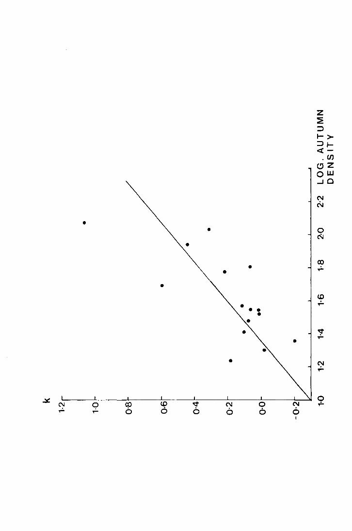
co 0

•

N 0

0 0

N

0

z ~ :::::> 1-> :::::>t-<(-.en

(.!)Z ow ...JO

N N

0 c\1

co

N ~

0 ,.:..

densities when plotted against each other both yield regression

coefficients that are significantly different from unity

(t = 3.50, p <::::. 0.01 and t = 2.62, p <. 0.02 respectively) and

it can therefore be concluded that overwinter mortality is

positively related to density.

5d. Overwinter mortality on Knock Fell in 1972

Other mortality factors such as diseas~ or parasit-

92

ization were not obvious on the Moor House sites. Coulson (1962)

describes a black discoloration of the epidermis which he attributed

to fungal attack, but as it can be induced in the laboratory by

puncturing the cuticle it could be the result of disease or physical

damage rather than the appearance of the infection itself. Both

during his study, when eight larvae were afflicted in a sample of

102, and during most of this study, very few blackened larvae

were found and it was not thought to be an important mortality

factor until a much higher density of infected larvae was found

on the Knock Fell site in spring 1972. On 9 March 1972

seventeen larvae from a sample of fifty five (30%) were

found to be discoloured. Of these seventeen larvae, eleven

were found dead (none of the normal larvae found in the same

sample were dead). The area was sampled three times; on

28 February 1972 before the mortality occurred, on 9 March 1972

when the dead larvae were found, and on 24 March 1972. Between

the first and the last date the population dropped significantly

(t = 2.64, p~O.Ol) showing a 45% mortality which could be

accounted for adequately by the percentage of dead and blackened

larvae found in early March. The data are presented in Table 28.

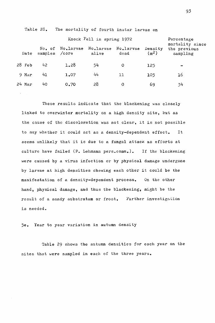
93

Table 28. The mortality of fourth instar larvae on

Knock Fell in spring 1972 Percentage mortality since

No. of No.larvae No.larvae No.larvae Density the previous Date samples /core alive dead (m2) sampling

28 Feb 42 1.28 54 0 125

9 Mar 41 1.07 44 ll 105 16

24 Mar 40 0.70 28 0 69 34

These results indicate that the blackening was closely

linked to overwinter mortality on a high density site, but as

the cause of the discoloration was not clear, it is not possible

to say whether it could act as a density-dependent effect. It

seems unlikely that it is due to a fungal attack as efforts at

culture have failed (P. Lehmann pers.comm.). If the blackening

were caused by a virus infection or by physical damage undergone

by larvae at high densities chewing each other it could be the

manifestation of a density-dependent process. On the other

hand, physical damage, and thus the blackening, might be the

result of a sandy substratum or frost. Further investigation

is needed.

5e. Year to year variation in autumn density

'l'able 29 shows the autumn densities for each year on the

sites that were sampled in each of the three years.

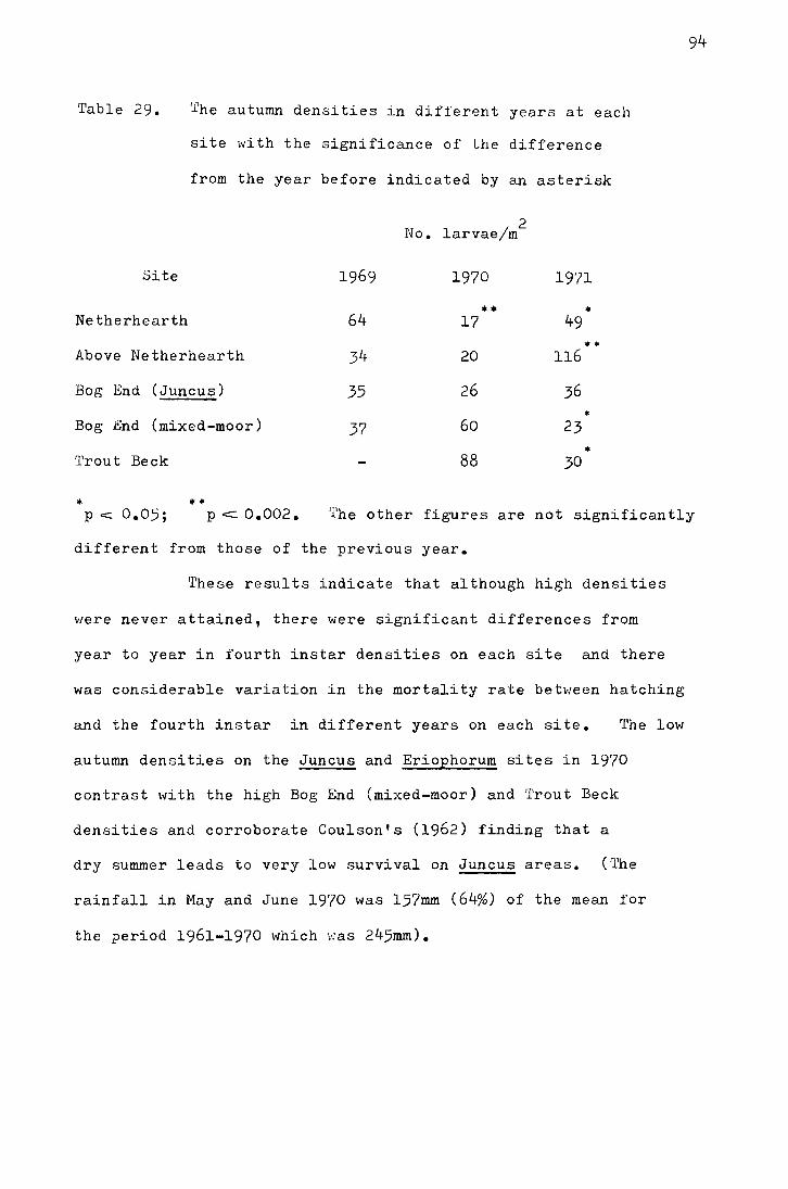
Table 29. 'i'he autumn densities in different years at each

site Hith the significance of the difference

from the year before indicated by an asterisk

Site 1969

Netherhearth 64

Above Netherhearth 34

Bog End (Juncus) 35

Bog End (mixed-moor) 37

Trout Beck

* **

2 No. larvae/m

1970

•• 17

20

26

60

88

1971

• 49

•• 116

36 * 23

* 30

94

p < 0.05; p <:. 0.002. The other figures are not significantly

different from those of the previous year.

These results indicate that although high densities

were never attained, there were significant differences from

year to year in fourth instar densities on each site and there

was considerable variation in the mortality rate between hatching

and the fourth instar in different years on each site. 'fhe low

autumn densities on the Juncus and Eriophorum sites in 1970

contrast with the high Bog End (mixed-moor) and Trout Beck

densities and corroborate Coulson's (1962) finding that a

dry summer leads to very low survival on Juncus areas. (The

rainfall in May and June 1970 was 157mm (64%) of the mean for

the period 1961-1970 \vhich 1:1as 245mm).

6'•Mortality rate during pupation

The mortality rate during pupation cannot be directly

calculated because the estimates of adult densities in this study

are not sufficiently accurate. However, there is evidence of

differential mortality between the sexes either late in the

fourth instar or during pupation and emergence. Inequality

in the sex ratio has been noticed in a number of tipulid species

(Coulson 1962, Freeman 1964, Hadley 1969). Coulson found a

1 : l larval sex ratio in T. subnodicornis on dissection in

95

March and attributed the preponderance of males in the adult

population to the greater longevity of the male which he estimated

from mark recapture data. Freeman, on the other hand, found

that the inequality of the sex ratio among adult !· luna

corresponded to a bimodality in larval head capsule and suggested

that the sex ratio was already unequal in the fourth instar.

In the present study 167 males and 68 females

emerged from the traps at Netherhearth in 1972 giving a ratio

of 2.46 males : l female. Searching for pupal cases within

the traps revealed 100 male and 39 female cases, giving a ratio

of 2.57 males : 1 female. The technique of estimating the

sex ratio (Coulson 1962) or emergence pattern (Laughlin 1967)

from pupal cases has been used for !· paludosa and it "'as felt

from the emergence trap data that an accurate estimate of the

sex ratio could also be made by the same method for !• subnodicornis.

Between 21 '1'1ay and 1 June 19'70, 272 pupal cases v1ere collected on

the Bog End (Juncus) site. 204 of these were male and 68 female,

a ratio of 3 : l and a significant departure from the 1 : l sex

96

·v2 ratio (_-'\. = 68, p <0.001, d. f. l). It was therefore concluded

that there was a real inequality in the sex ratio of emerging

adults and that this was due to differential mortality in the

very late larval stage or during pupation and emergence rather

than to a larval inequality established in the last instar as

in .:£. luna. Further evidence to support this view was derived

from the laboratory cultures in which 293 fourth instar larvae

gave rise to 121 males and 142 females. This result does not

differ significantly from a l l ratio <X.2 = 1.68, p>O.l,

d.f. l) and indicates that in a favourable environment differential

mortality does not occur to the extent that it does in the field.

7 • Conclusion

There is both field and experimental evidence to

indicate that mortality in a number of crane-flies is closely

linked to weather conditions at specific stages in the life-

history. The egg and first instar appear to be particularly

susceptible to drought and Milne et al. (1965) correlated poor

survival of T. paludosa with drought in the early autumn and

showed experimentally that the egg or hatching stage was more

vulnerable than the first instar. Coulson (1962) suggested

that drought caused the population crash of T. subnodicornis

in 1955 and showed that in this case the hatching success was

normal and that the first instar succumbed. The high first

instar mortality was confirmed in this study when a 98%

mortality was found by 28 July 1972 on Knock Fell and the

low densities of larvae on Juncus sites after the dry summer in

1970 agree with his finding that after the drought in 1955 the

densities of larvae on the Juncus areas were drastically reduced

whilst those on blanket-bog were relatively unaffected.

Overwinter mortality has been measured and it is

not thought that, over the period of this study, it was caused

primarily by low temperature as the larvae appeared to be

sufficiently cold-hardy to survive temperatures encountered

a few centimetres below the ground surface.

The effect of density on mortality has been examined

experimentally for the early instars and in the field for fourth

instar larvae. It has been shown that both in the early instars

and in the overwintering stage mortality is higher at high

densities. First instar larvae in culture were often seen

biting each other, but a. chewed larva was usually dead by

the time it was observed. Laughlin (1958) found a considerable

degree of cannibalism in 'I'. oleracea larvae and this may well

account for mortality of crowded first instar T. subnodicornis

larvae in the field. In the later instars there was no evidence

of the larvae in culture damaging each other, so it \'IOuld seem

unlikely that this could be a factor in the over-winter mortality

in the field. It is more likely that during cold periods thase

larvae that fail to find a refuge are at risk. It has been

shown that the larvae need migrate to a depth of only a few

centimetres in Juncus litter to avoid extreme low temperature,

but the number of positions where conditions are suitable during

a period of alternate thawing and freezing conditions may be

limited. If this were the case, a marked density effect would

be expected.

97

Further effects of density, on the size of larvae,

have also been observed, and are discussed in the following

section which deals with wing length. The possib~lity that

numbers of T. subnod~cornis on a site could be lim~ted by the

food supply is examined in the next section.

98

XII.Analysis of gut contents for 1:_. subnodicornis and 'I'. var~ipennis Me..t:.'l"-''

Coulson (1962) found that there was a significantly

higher density of 1:_. subnod~cornis larvae in samples containing

Diplophyllum albicans and Ptilidium ciliare than in samples from

which li verv:orts were absent when he sampled the Eriophorum sward

at Netherhearth in 1954. He also found that liverworts constituted

the majority of identifiable remains in the faeces. Freeman ( 1967),

on the other hand, studied the feeding of ten species of tipulid

larvae and found no evidence of selection for food within groups

of larvae taken from the same type of habitat. He therefore

concluded that competition for food was not an "important factor

in their ecology". As the densities of T. subnodicornis on

areas of the Noor House Reserve are on occasion very high, and

the supply of liverworts limited,a further analysis of the

larval diet was made. The 2550ft site on Knock Fell was

chosen as a suitable area to sample on the grounds that not

only was there a high density of !• subnodicornis, but that

1:_. variipennis was also present so that any selectivity in

the two species could be compared.

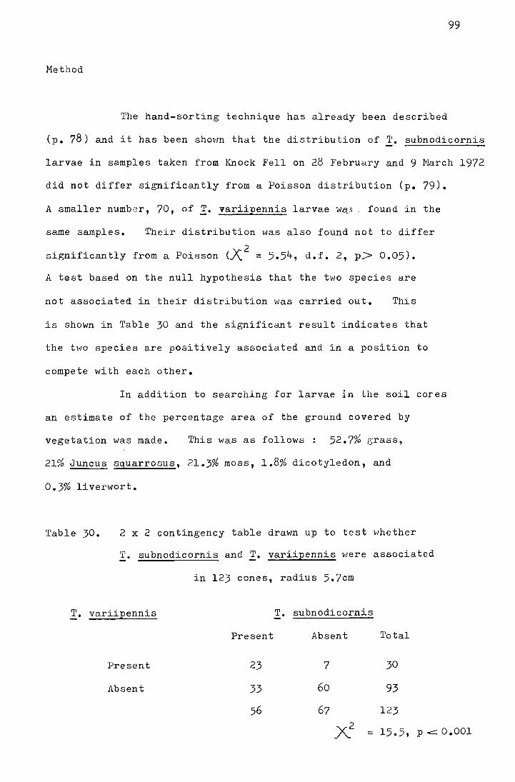
99

Method

The hand-sorting technique has already been described

(p. 78) and it has been shO\m that the distribution of 1'. subnodicornis

larvae in samples taken from Knock Fell on 28 February and 9 March 1972

did not differ significantly from a Poisson distribution (p. 79).

A smaller number, 70, of !· variipennis larvae was . found in the

same samples. Their distribution was also found not to differ

. x2 significantly from a Po~sson ( = 5.54, d.f. 2, p:> 0.05).

A test based on the null hypothesis that the two species are

not associated in their distribution was carried out. This

is shown in Table 30 and the significant result indicates that

the two species are positively associated and in a position to

compete with each other.

In addition to searching for larvae in the soil cores

an estimate of the percentage area of the ground covered by

vegetation was made. This was as follows : 52.7% grass,

21% Juncus squarrosus, 21.3% moss, 1.8% dicotyledon, and

0.3% liverwort.

Table 30. 2 x 2 contingency table drawn up to test whether

T. subnodicornis and !· variipennis were associated

in 123 cones, radius 5.7cm

T. variipennis T. subnodicornis

Present Absent 1'otal

Present 23 7 30

Absent 33 60 93

56 67 123

x2 = 15.5, p.:::::::O.OOl

100

The guts of 35 !· subnodicornis and 13 !• variipennis

larvae 1·1ere removed and the contents teased out on a slide and

examined wet, Hi th no further preparation, under high pmver.

Results

The categories that the plant tissues and other gut

contents have been divided into, and the number of occurrences

in each category, have been listed below in Table 31. Only in cases

where the characteristic epidermal cells were present have pieces

of tissue without chlorophyll been classified as leaf, and only

where root hairs were present were tissues listed as root.

This leaves a large proportion of the gut contents in both

species that can only be classified as miscellaneous plant

tissue. It is not, therefore, possible to compare the

proportions of the vegetation available and the proportions

in the gut.

As no attempt to assess the size of pieces ingested

was made, it was thought more relevant to compare the number of

occurrences in the guts of each of the two species rather than

to compare the proportions of the different tissues in the guts.

2 )\ has been calculated separately for each category on the basis

that the type of vegetation should occur in the same number of

guts, proportionally, for both species. The results of this

analysis are shown in the last column of Table 33. The number

of !· varfipennis guts containing grass and higher plant tissue

is significantly greater than that of !• subnodicornis, and it

can be seen from Table 31 that mosses constitute a higher

percentage of all the pieces examined from the T. subnodicornis

than they do of the !· variipennis guts. ~hese differences

may be the result of the difference in mandible size in the two

species (that of T. subnodicornis is two thirds the length of

that of !· variipennis) and are consistent with the habitat

preferenceSof the two. T. subnodicornis is found primarily

on peat and ~· variipennis is found primarily on alluvial soils

101

or mixed peat and alluvial areas (Coulson 1959). As both species

are polyphagous and the food is apparently abundant, it is unlikely

that either species is directly limited by the food supply or that

they come into competition for this resource. However, at high

densities the difference in their primary food choice would allow

them to co-exist.

i

'

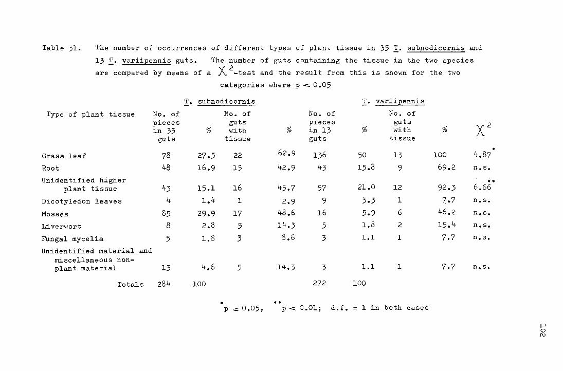
Table 31. The number of occurrences of different types of plant tissue in 35 !· subnodicornis and

13 !• variipennis guts. The number of guts containing the tissue in the two species

are compared by means of a A 2 -test and the result from this is shown for the two

categories where p < 0.05

T. subnodicornis !• variipennis

Type of plant tissue No. of No. of No. of No. of pieces guts pieces guts x2 in 35 % with ol in 13 % with % /0

guts tissue guts tissue

Grass. leaf 78 27.5 22 62.9 136 50 13 100 4.87

Root 48 16.9 15 42.9 43 15.8 9 69.2 n.s.

•

Unidentified higher •• plant tissue 43 15.1 16 45.7 57 21.0 12 92.3 6.66

Dicotyledon leaves 4 1.4 1 2.9 9 3.3 1 7.7 n.s.

Mosses 85 29.9 17 48.6 16 5.9 6 46.2 n.s.

Liverwort 8 2.8 5 14.3 5 1.8 2 15.4 n.s.

Fungal mycelia 5 1.8 3 8.6 3 1.1 1 7.7 n.s.

Unidentified material and miscellaneous non-plant material 13 4.6 5 14.3 3 1.1 l 7.7 n.s.

Totals 284 100 272 100

• *"' p c:::::- 0.05, p < 0.01; d.f. = 1 in both cases

1-' 0 !\.)

XIII. Variation in size and fecundity in ~. subnodicornis

in the field and under experimental conditions

When the fecundity of !· subnodicornis was being

studied in 1969 (M.Sc. dissertation) it proved impossible to

find adequate numbers of teneral females on each site. 'ihe

counting of eggs in individual females was also time-consuming

so a parameter that would reflect egg number vras sought. Wing,

tibia and tarsus lengths were measured for a sample of teneral

females and these measurements correlated vli th egg numbers and

3/ egg numbers/female. It was found that the relationship

beh1een wing length and 3/ egg numbers gave the highest

correlation coefficient (r =t-0.613, p-===: 0.001).

In the present study some parameter that reflected

fecundity vtas again sought so that this means of population

change could be studied. It is generally accepted (Hemmingsen

and Birger Jensen 1960) that the relationship of the size of

the part of an organism vli th another is best expressed by

such an equation as log y = log x b + log a, where y and x

are measurements of body lengths, b is the slope and a the

intercept on the y axis. In the case of the wing measurement

it would be expected that wing area would be proportional to

the weight of a fly and therefore a more relevant measurement

than wing length. Hovrever, as the measurement of area would

have been a complex procedure, it was decided to determine

whether wing length alone could be used to indicate weight.

Femur length, the only conveniently measured parameter not

investigated in 1969, has also been related to weight.

103

104

1. The relationship of wing a.nd femur length with dry weight

Flies that were used for dry weight estimates were

collected from the site and killed by a short exposure to

ethyl acetate. They were then brought back to the laboratory,

measured under a low power microscope with a scale in the eyepiece,

0 and dried to constant weight in a vacuum oven at 40 C. The results

of the correlations between wing length, femur length, the logarithms

of these measurements and dry \veight, 3./dry weight and the

logarithms of these measurements for flies caught on the 1900ft

site on Dun Fell are shown in Table 32. Male flies have been

used to avoid the complication of the uncertainty as to how

many eggs the females have laid. The normality of wing length

distribution for flies on a site has been checked by plotting

the wing lengths of 199 males and 222 females from pitfalls at the

2500ft site in 1967 on normal probability paper. This is

shown in fig. V in the appendix.

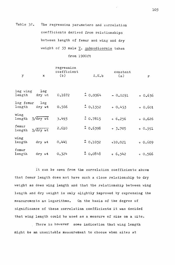
Table 32.

y

'l'he regression parameters and correlation

coefficients derived from relationships

between length of femur and wing and dry

vJeigh t of 33 male 'I'. subnodicornis taken

X

from l900ft

regression coefficient

(b) S.E.b constant

(a)

105

r

log v1ing length

log dry Ht 0.1672 +

- 0.0364 - 0.0291 + 0.636

log femur length

wing

log dry wt

length 3/dry wt

femur length 3/dry wt

wing length dry wt

femur length dry wt

0.566

3.493

2.610

0.441

0.324

+ - 0.1352 + 0.453 + 0.601

+. 6.256 + 0.626

+ 0.6398 + 3.705 + 0.591

+. 0.1032 +10.021 + 0.609

+ o.o848 + 6.542 + 0.566

It can be seen from the correlation coefficients above

that femur length does not have such a close relationship to dry

weight as does wing length and that the relationship betHeen wing

length and dry weight is only slightly improved by expressing the

measurements as logarithms. On the basis of the degree of

significance of these correlation coefficients it was decided

that wing length could be used as a measure of size on a site.

There is however some indication that wing length

might be an unsuitable measurement to choose when sites at

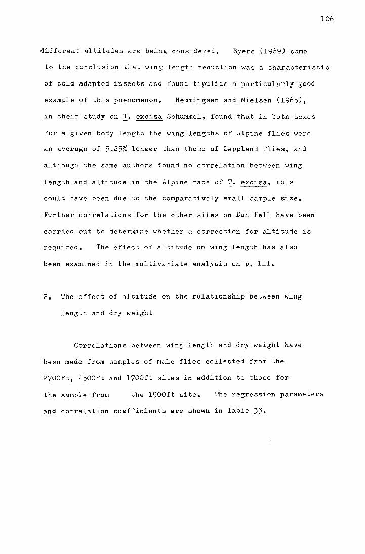
106

different altitudes are being considered. Byers (1969) came

to the conclusion that wing length reduction was a characteristic

of cold adapted insects and found tipulids a particularly good

example of this phenomenon. Hemmingsen and Nielsen (1965),

in their study on ,:!:. excisa Schummel, found that in both sexes

for a given body length the wing lengths of Alpine flies were

an average of 5.25% longer than those of Lappland flies, and

although the same authors found no correlation between wing

length and altitude in the Alpine race of.:!:.· excisa, this

could have been due to the comparatively small sample size.

Further correlations for the other sites on Dun Fell have been

carried out to determine whether a correction for altitude is

required. The effect of altitude on wing length has also

been examined in the multivariate analysis on p. 111.

2. The effect of altitude on the relationship between wing

length and dry weight

Correlations between wing length and dry weight have

been made from samples of male flies collected from the

2700ft, 2500ft and 1700ft sites in addition to those for

the sample from the 1900ft site. The regression parruaeters

and correlation coefficients are shown in Table 33.

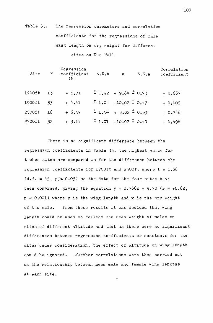
107

Table 33. The regression parameters and correlation

coefficients for the regressions of male

wing length on dry weight for different

sites on Dun Fell

Site N Regression coefficient

(b) a S.E.a

Correlation coefficient

l700ft

l900ft

2500ft

2700ft

13

33

16

32

+ 5.71

+ 4.41

+ 6.59

+ 3.17

! 1.92 + 9.64 ! 0.73

+ 1.04 +.10.02 + 0.47

+ + 1.54 + 9.02 - 0.53

+ 1.01 +10.02 + o.4o

+ 0.667

+ 0.609

+ 0.746

+ 0.498

There is no significant difference between the

regression coefficients in Table 33, the highest value for

t when sites are compared is for the difference between the

regression coefficients for 2700ft and 2500ft where t = 1.86

(d.f. = 45, p~ 0.05) so the data for the four sites have

been combined, giving the equation y = 0.786x + 9.70 (r = +0.62,

p ~ 0.001) where y is the wing length and x is the dry weight

of the male. From these results it was decided that wing

length could be used to reflect the mean weight of males on

sites of different altitude and that as there were no significant

differences between regression coefficients or constants for the

sites under consideration, the effect of altitude on wing length

could be ignored. ~urther correlations were then carried out

on the relationship between mean male and female wing lengths

at each site.

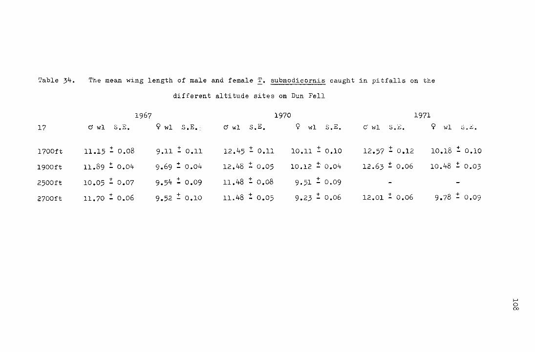
Table 34.

17

l700ft

l900ft

2500ft

2700ft

The mean wing length of male and female J. subnodicornis caught in pitfalls on the

different altitude sites on Dun Fell

1967 1970 1971

Cf wl s c;' ........ 9 wl S .E.: Cf wl s.E. 9 wl s.E. o' wl s.~. 9 wl S.E.

11.15 :!: o.o8 + 9.11 - O.ll + 12.45 - 0.11 + 10.11 - 0.10 + 12.57 - 0.12 10.18 :!: 0.10

11.89 :!: 0.04 9.69 :!: 0.04 12.48 :!: 0.05 10.12 :!:· 0.04 12.63 ! 0.06 10.48 :!: 0.03

+ 10.05 - 0.07

+ 9.54 - 0.09 11.48 :!: o.o8 9.51 :!: 0.09

11.70 ~ 0.06 + 9.52 - 0.10 11.48 : 0.05 9.23 : o.o6 12.01 :!: o.o6 9.78 :!: 0.09

f--' 0 co

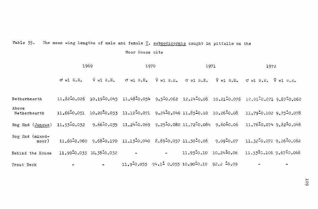
Table 35. The mean wing lengths of male and female T. subnodicornis caught in pitfalls on the

Moor House site

1969 1970 1971 1972

d wl S.E. 9 wl s.E. d wl s.E. 9 wl S.E. 0 wl s.E. 9 wl s.E. d wl s.~. 9 wl ~-~-

Netherhearth 11.82:0.026 10.19:0.045 11.48:0.054 9.5:0.062 12.24:o.o8 10.21:0.076 + 8 + 12.01-0.071 9. 7-0.062

Above Netherhearth 11.66:0.051 + 10.20-0.033 11.12:0.071 + 8 + 9.24-0.046 11. 5-0.10 10.26:o.o8 + + 8 11.79-0.102 9.75-0.07

Bog End (Juncus) + 11.53-0.032 9.66:0.035 11.24:0.069 + + 8 9.25-0.080 11.72-0.0 4 9.6o:!:o.o6 11.76:o.o74 9.82:!:o.o48

Bog End (mixed-11.6o:o.o6o 9.68:0.170 11.13:0.040 8.89:0.057 11.5o!o.o8 + 11.32:0.072 9.26:!:0.082 moor) 9.09-0.07

11.99:0.035 10. 38:o. o 32 + 10.24:!:0.06 11.53:!:0.106 9.67:!:o.o68 Behind the House - - 11.93-0.10

+ + + + Trout Beck - - 11.9-0.055 94.1- 0.055 10.90-0.10 92.2 -0.09

I-' 0 '-()

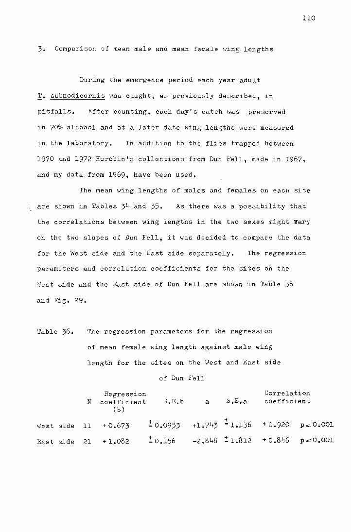
110

3. Comparison of mean male and mean female 1·1ing lengths

During the emergence period each year adult

T. subnodicornis was caught, as previously described, in

pitfalls. After counting, each day's catch was preserved

in 70% alcohol and at a later date Hing lengths 1-1ere measured

in the laboratory. In addition to the flies trapped between

1970 and 1972 Horobin's collections from Dun Fell, made in 1967,

and my data from 1969, have been used.

The mean wing lengths of males and females on each site

are shown in Tables 34 and 35. As there was a possibility that

the correlations between wing lengths in the two sexes might Yary

on the two slopes of Dun Fell, it was decided to compare the data

for the West side and the East side separately. 'l'he regression

parameters and correlation coefficients for the sites on the

West side and the East side of Dun Fell are shown in Table 36

and Fig. 29.

Table 36. The regression parameters for the regression

of mean female wing length against male wing

length for the sites on the \Jest and East side

of Dun Fell

Regression Correlation N coefficient 0.E.b a ::;.E.a coefficient

(b)

1:'/est side ll + 0.673 + - 0.0953 +1.743

+ - 1.136 + 0.920 p-c::::. 0.001

East side 21 + 1.082 ~ 0.156 -2.848 ~ 1.812 + 0.846 p.:::::.-0.001

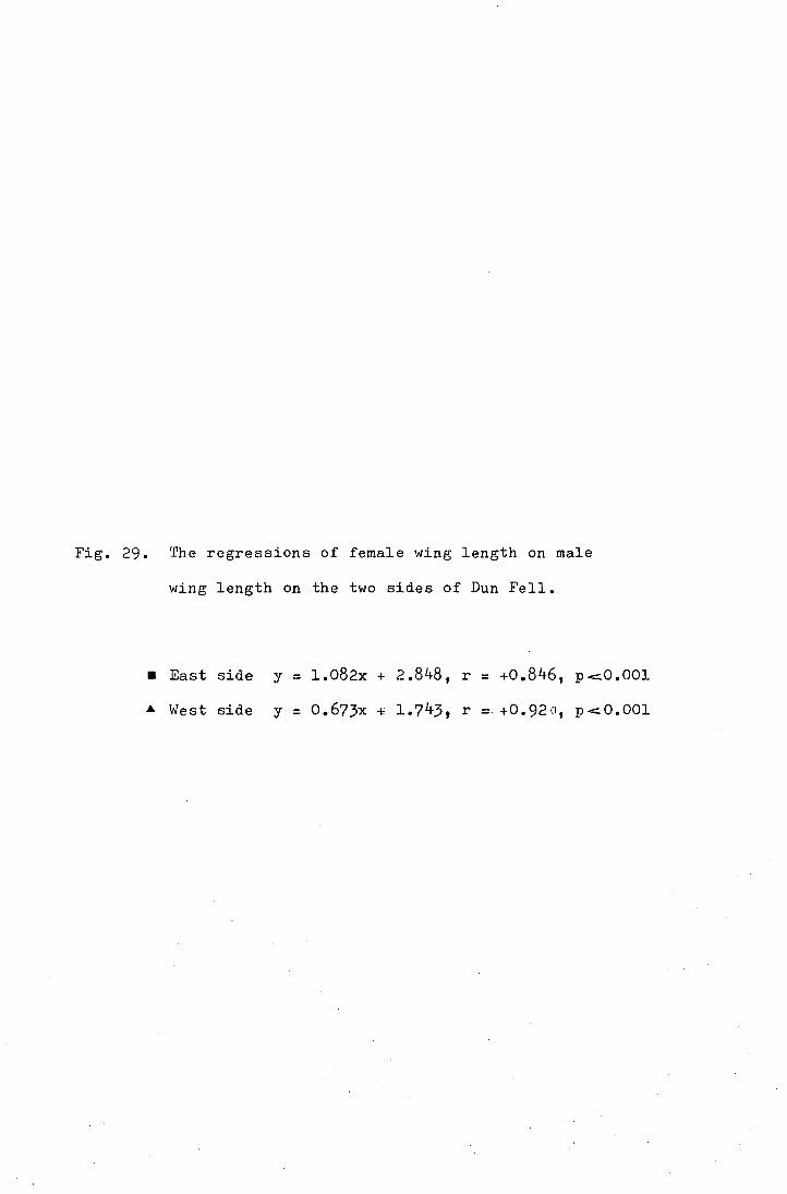
Fig. 29. The regressions of female wing length on male

wing length on the two sides of Dun Fell.

• East side y = l.082x + 2.848, r = +0.846, pc:::.::.O.OOl

• West side y = 0.673x + 1.743, r- +0.92o, p..:::.O.OOl

• • • •

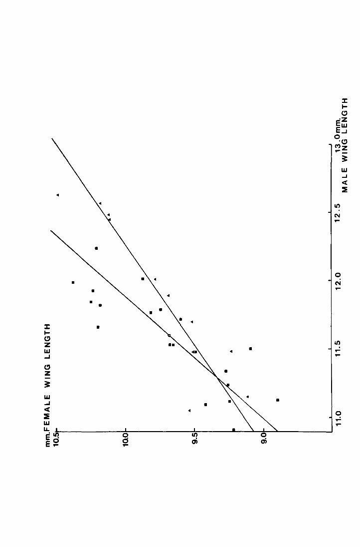
... :I: • t-

" z w ..J

" z 3r: w ..J < ... :IE w LL.

'LI) 0 Ll) E • E~ d a,

~

... •

•

• •

:I: t­o ·z Ew

E..J 0 ·o Mz ~

0 N ~

Ll)

~

~

0 ~

~

w ..J < :IE

111

Both the regression coefficients and the constants are significantly

different on either side of Dun Fell (t = 2.24 d.f. 30, p < 0.05

and 2.15 d.f. 30, p < 0.02) respectively. 'l'he information

therefore has not been combined, but it was concluded that the

relationships between male and female wing length on the two

sides were closely correlated for the wing length of either sex

to be used as an indication of size on a site from the appropriate

side of Dun Fell.

4. Multivariate analysis on the factors affecting wing length

Further information on the variation of wing length

from year to year and from site to site has been extracted by

means of a. multivariate analysis. The programme used was a

Stepwise Regression, coded BMD02R (Dixon 1968).

The effect of the following variables on wing length

has been tested : year, site, altitude and density. It was

thought that autumn or spring larval density might bear a closer

relation to the weight of the adult than the pitfall catch which,

if there has been any mortality, will not represent the density

during the larval growth period. As there were no larval density

measurements for the West side, the two sides have, in the first

instance, been considered separately. The blanket-bog sites

have not been used, and the Behind House site in 1972, when it

was flooded, has been omitted. A list of variables entered on

each run is shown below in Table 37. The larval densities were

taken from Table XI in the appendix· and the adult densities from

the pitfall data in Tables XII and XIII in the appendix.

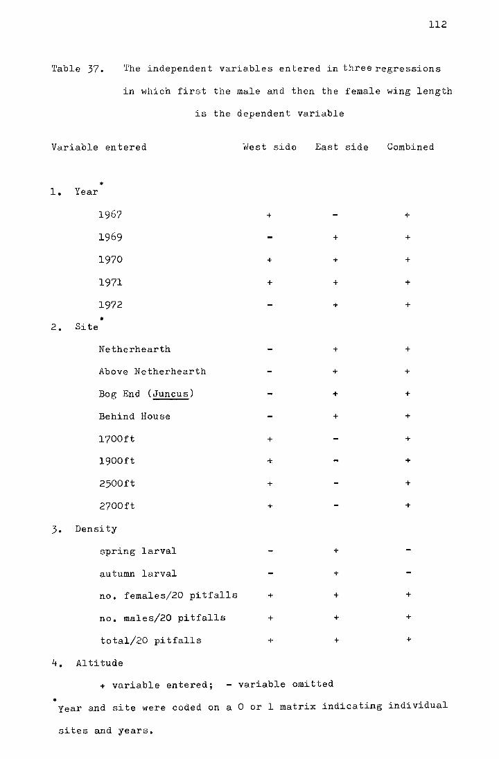
112

'l'able 37. 'l'he independent variables entered in three regressions

in which first the male and then the female wing length

is the dependent variable

Variable entered

• 1. Year

2. Site

1967

1969

1970

1971

1972

*

Netherhearth

Above Netherhearth

Bog End (Juncus)

Behind House

l700ft

l900ft

2500ft

2700ft

3. Density

spring larval

autumn larval

no. females/20 pitfalls

no. males/20 pitfalls

total/20 pitfalls

4. Altitude

-vJest side East side

+

+

+ +

+ +

+

+

+

+

+

+

+

+

+

+

+

+ +

+ +

+ +

+ variable entered; - variable omitted

Combined

+

+

+

+

+

+

+

+

+

+

+

+

+

+

+

+

• Year and site were coded on a 0 or l matrix indicating individual

sites and years.

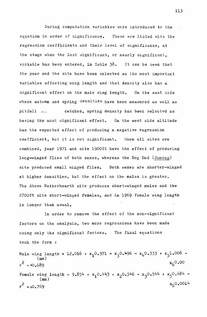
113

During computation variables were introduced to the

equation in order of significance. These are listed with the

regression coefficients and their level of significance, at

the stage when the last significant, or nearly significant,

variable has been entered, in Table 38. It can be seen that

the year and the site have been selected as the most important

variables affecting wing length and that density also has a

significant effect on the male wing length. On the east side

where autumn and spring densities have been measured as vJell as

pitfall .cc catches, spring density has been selected as

having the most significant effect. On the west side altitude

has the expected effect of producing a negative regression

coefficient, but it is not significant. When all sites are

combined, year 1971 and site l900ft have the effect of producing

long-winged flies of both sexes, whereas the Bog End (Juncus)

site produced small winged flies. Both sexes are shorter-winged

at higher densities, but the effect on the males is greater.

The Above Netherhearth site produces short-winged males and the

2700ft site short-winged females, and in 1969 female wing length

is longer than usual.

In order to remove the effect of the non-significant

factors on the analysis, two more regressions have been made

using only the significant factors. The final equations

took the form :

Male wing length (mm)

2 r =-!{) .689

= 12.016 + x 10.371 - x30.496 - x 40.333 + x

5l.008 -

x6o.oo

Female wing length = 9.854 + x 1o.443 + x 20.546 - x3o.544 + x

5o.684 -

(mm) 2 x 6o.OOl4

r =+0.769

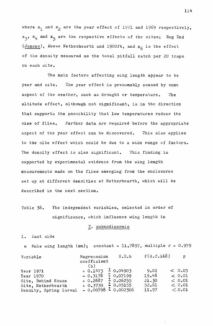
114

where x1 and x 2 are the year effect of 1971 and 1969 respectively,

x3

, x 4 and x5

are the respective effects of the sites; Bog End

(Juncus), Above Netherhearth and l900ft, and x6

is the effect

of the density measured as the total pitfall catch per 20 traps

on each site.

The main factors affecting wing length appear to be

year and site. The year effect is presumably caused by some

aspect of the weather, such as drought or temperature. The

altitude effect, although not significant, is in the direction

that supports the possibility that low temperatures reduce the

size of flies. Further data are required before the appropriate

aspect of the year effect can be discovered. This also applies

to the site effect which could be due to a wide range of factors.

The density effect is also significant. This finding is

supported by experimental evidence from the wing length

measurements made on the flies emerging from the enclosures

set up at different densities at Netherhearth, which will be

described in the next section.

Table 38. The independent variables, selected in order of

significance, which influence wing length in

'1.'. subnodicornis

l. E;ast side

a Hale wing length (mm); constant= 11.7897, multiple r = 0.979

Variable Regresssion s.E.b F' (d. f.l&8) p coefficient

(b) +

Year 1971 + O.lL~73 - 0.04903 9.02 ..:::::. 0.05 Year 1970 - 0.3178

+ 0.07199 19.48 0.01 - < Site, Behind House + 0.2887 + 0.06255 21.30 .::::::: 0.01 -

+ 0.3739 + 0.05155 52.61 ~ 0.01 Site, Netherhearth -+

Density, Spring larval - 0.00798 - 0.002306 11.97 -:::::::. o.o1

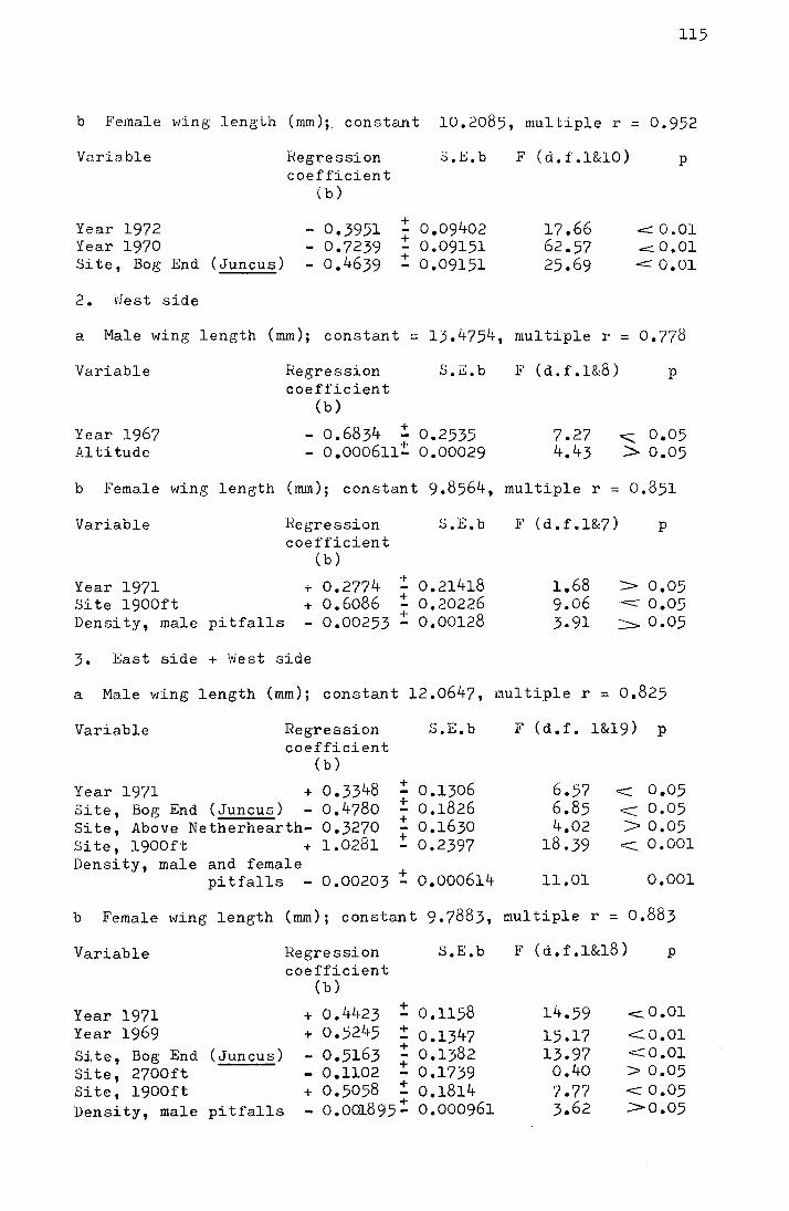
115

b Female vting length (mm ); constant 10.2085, multiple r = 0.952

Variable Regression s.E.b F (d.f.l&lO) p coefficient

(b)

Year 1972 - 0.3951 + 0.09402 17.66 - .::::: 0.01

Year 1970 - 0.7239 + 0.09151 62.57 ...:::::. o.o1 -

Site, Bog End (Juncus) - 0.4639 + 0.09151 25.69 . ..:::::: o.o1 -

2. \ilest side

a Male wing length (mm); constant = 13.4754, multiple r = 0.778

Variable Regression S.:2;.b F' (d. f.l&8) p coefficient

(b)

Year 1967 - 0.6834 + 0.2535 7.27 0.05 - ...;;;:

Altitude - o.ooo611:!: 0.00029 4.43 > 0.05

b Female wing length (mm); constant 9.8564, multiple r = 0.851

Variable

Year 1971 Site l900ft Density, male pitfalls

Regression coefficient

(b)

+ 0.2774 + o.6o86 - 0.00253

3. East side + West side

s.E.b

+ 0.21418 + 0.20226 + 0.00128

F (d.f.l&7)

1.68 9.06 3.91

p

> 0.05 --=:::::- 0.05

:::::::::. 0.05

a Male wing length (mm); constant 12.0647, multiple r = 0.825

Variable Regression coefficient

(b)

s.E.b

+ 0.1306 + 0.1826 + 0.1630 + 0.2397

Year 1971 + 0.3348 Site, Bog End (Juncus) - 0.4780 Site, Above Netherhearth- 0.3270 Site, l900ft + 1.0281 Density, male and female

+ pitfalls - 0.00203 0.000614

F (d.f. 1&19) p

6.57 6.85 4.02

18.39

11.01

< 0.05 < 0.05 > 0.05 <. 0.001

0.001

b Female wing length (mm); constant 9.7883, multiple r = 0.883

Variable

Year 1971 Year 1969

Site, Bog End (Juncus) Site, 2700ft Site, 1900ft Density, male pitfalls

Regression coefficient

(b)

+ 0.4423 + + 0.5245 +

+ - 0.5163 -+ - 0.1102 + 0.5058 +

+ - 0.001895-

s.E.b

0.1158

0.1347 0.1382 0.1739 0.1814 0.000961

F (d. f.l&l8 ) p

14.59

15.17 13.97 o.4o 7.77 3 .. 62

<.0.01

<0.01 <0.01 > 0.05 < 0.05 >0.05

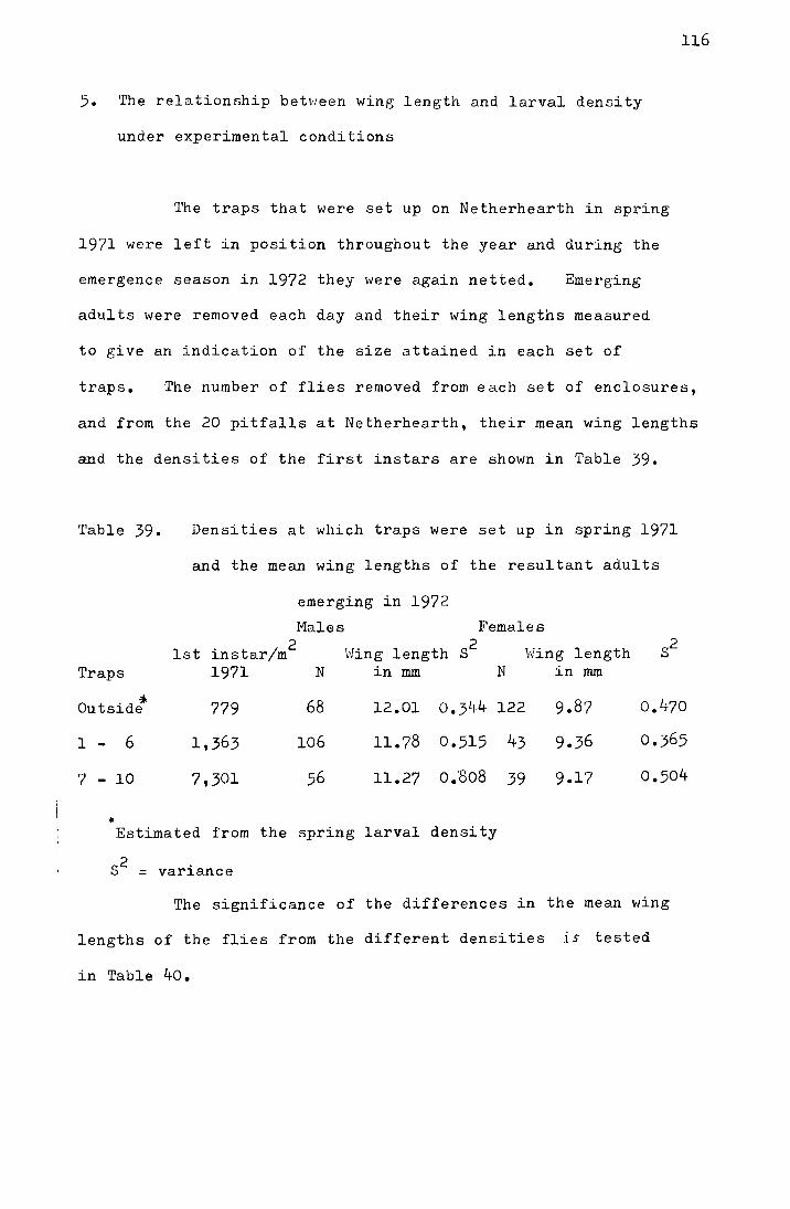
116

5. The relationship between wing length and larval density

under experimental conditions

The traps that were set up on Netherhearth in spring

1971 were left in position throughout the year and during the

emergence season in 1972 they were again netted. Emerging

adults were removed each day and their wing lengths measured

to give an indication of the size attained in each set of

traps. The number of flies removed from each set of enclosures,

and from the 20 pitfalls at Netherhearth, their mean wing lengths

and the densities of the first instars are shown in Table 39.

Table 39. Densities at which traps were set up in spring 1971

and the mean wing lengths of the resultant adults

emerging in 1972

Males Females

1st instar/m2 Hing length s2 hiing length s2

Traps 1971 N in mm N in mm

Outsidl 779 68 12.01 0.344 122 9.87 0.470

1 - 6 1,363 106 11.78 0.515 43 9.36 0.365

7 - 10 7,301 56 11.27 o.'8o8 39 9.17 0.504

* Estimated from the spring larval density

s 2 = variance

The significance of the differences in the mean v1ing

lengths of the flies from the different densities is tested

in Table 40.

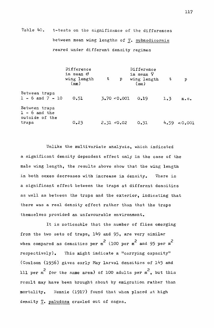
117

'l'able 40. t-tests on the significance of the differences

between mean wing lengths of !· subnodicornis

reared under different density regimes

Difference Difference in mean d in mean 9 wing length t p wing length t p

(mm) (mm)

Between traps l - 6 and 7 - 10 0.51 3.70 .:::-0.001 0.19 1.3 n.s.

Between traps l - 6 and the outside of the traps 0.23 2.31 <0.02 0.51 4.59 <0.001

Unlike the multivariate analysis, which indicated

a significant density dependent effect only in the case of the

male wing length, the results above show that the wing length

in both sexes decreases with increase in density. There is

a significant effect between the traps at different densities

as well as between the traps and the exterior, indicating that

there was a real density effect rather than that the traps

themselves provided an unfavourable environment.

It is noticeable that the number of flies emerging

from the two sets of traps, 149 and 95, are very similar

when compared as densities per m2

(100 per m2

and 95 per m2

respectively). This might indicate a "carrying capacity"

(Coulson (1956) gives early May larval densities of 145 and

2 2 lll per m for the same area) of 100 adults per m , but this

result may have been brought about by emigration rather than

mortality. l~ennie (1917) found that when placed at high

density!· paludosa crawled out of cages.

Conclusion

It is concluded that high density is not only

associated with increased mortality but also with reduction

in wing length in adults. As wing length is correlated with

weight and fecundity it is assumed that at high densities there

will be a reduction in fecundity. The reduction of mean fecundity

associated with a decrease of mean female wing length from 9.87mm

to 9.17mm would be from approximately 280 eggs/female to 205 eggs/

female (M.Sc. dissertation). Although this is a 27% decrease

in the numbers entering the next generation it is unlikely that

reduction in numbers at this stage will have a great effect on

the regulation of adult density.

As the larvae are polyphagous, it seems unlikely

that the food supply would prove limiting on a site. It is

possible that the density effect is brought about by contact

between larvae as in Bupalus piniarius (Klomp and Gruys 1965;

Gruys 1970).

118

119

General discussion

This study has largely been concerned with two aspects

of the biology of !· subnodicornis ; the synchronisation of the

annual life-cycle and the fluctuation in numbers in the field.

The influence of temperature and photoperiod on the timing of

the life-history has been examined both in the field and the

laboratory. The variation of population density from year

to year and from site to site has been observed in the field

and the effect of density on mortality has been observed under

experimental conditions.

The response to temperature is such that both the

increase of g-rowth rate with temperature and the temperature

range over which this increase is shown, diminish during larval

development. The reduced response to temperature has been shown

to occur in the moth Dasychira pudibunda by Geyspitz and Zarankina

(1963) and the reduction in the range over which the response is

made is brought about in other insects such as Calandra oryzae

and Rhizopertha dominica (Birch 1944) as it is in T. subnodicornis

by the drop in the optimum temperature for development. Laughlin

(1963) found that during the development of Phyllopertha horticola

the lower temperature threshold dropped during development so that

although during the first instar larvae shoHed a slower growth and

lower survival rate at 12°C, in the second instar the rate of

development was as fast at 12°C as at 16° and 18°C. Although

the position of the lower threshold has not been determined for

!· subnodicornis, the situation is analagous in that in the fourth

0 0 0 instar the growth rate at 20 C is below that at 15 or 10 C.

Laughlin suggested that the drop in threshold temperature was an

adaptation to the· falling autumn temperature in the field. In

the case of T. subnodicornis the drop in the optimum temperature

for development would enable the larvae in the colder areas to

complete their growth not long after those in warmer habitats.

The next phase in development is temperature independent, or

possibly inversely related to temperature, and all larvae should

be in this stage by the end of the winter.

120

It is suggested that the main response to photoperiod

in T. subnodicornis comes in the fourth instar when the growth

period has finished, but that there may be a secondary response

during the growing period when larvae kept on a short photoperiod

grow more quickly than those on a long photoperiod. This could

be an adaptation promoting the development of larvae that have

not completed trteir growth by autumn due to their early development

having been retarded by low temperature.

The primary photoperiod effect lies in the response of

the full grown larvae to lengthening day which promotes and

synchronises pupation. The temperature independent phase takes

place on a short day length and, like some diapause conditions

(Beck 1968), can be broken by the appropriate photoperiod. If

larvae are taken from the field in mid December and kept at l0°C

they can be prevailed upon to pupate forty days earlier on an

eighteen hour day than on a six hour day. By the end of February

this effect has almost disappeared and the mean dates of pupation

are only seven days apart on the two light regimes. The variance

is, however, still significantly greater on the short day regime

and this suggests that the photoperiod effect may be additive

so that by the end of February, although the day length is long

enough to sychronise pupation to a certain extent, a longer

121

photoperiod has a greater effect. This type of situation exists

in !· pagana where both the mean ~upation date and the variance

decrease with shorter day length, and appears to be similar to

the effect found in the lacewing Chrysopa carnea Stephens(Tauber and

Tauber 1973) where the duration of the overwinter reproductive

diapause shows an inverse linear relationship with day length.

In the two tipulids studied it could be a useful adaptation

acting to accelerate the pupation of any larvae that have been

delayed in development or have failed to receive e~rlier photo­

period stimulation.

Most Tipulidae are characterised by their lack of

resistance to desiccation and many species within the group are

confined to areas where the humidity is high. This limitation

in habitat could be expected to impose severe restrictions on

the abundance of the species. However, in the two species studied,

T. subnodicornis and !· pagana, there are adaptations in the life­

histories that allow them to exist over a Hide temperature range

(therefore latitude and altitude), so suitable habitats can be

exploited over a large area.

Coulson and vlhi ttaker (in press) suggest that the fauna

at Moor House consists of two components; the moorland community

which has affinities with the fauna of northern Scandinavia, and

the grassland community which consists largely of species common

at lower altitudes. T. subnodicornis belongs to the first group

and !· pagana to the second. It is appropriate that the two species,

both showing adaptations that allow the annual cycle to be maintained

over a considerable latitude range, should both exist in an area

Hhere the two communiU.es are at the limits of their respective

ranges.

Z· subnodicornis is particularly interesting in that

it lacks a diapause. There is a considerable body of research

on the effect of temperature on the distribution and abundance

of animals (Andrewartha and Birch, 1954; Krebs 1972). The

ability of an animal to exist over a wide temperature range is

usually attributed to the presence of different genetic strains,

acclimatisation (Bullock 1955; Fry 1958) or, in the case of

insects, a diapause (Danilevskii 1965). However, in a number

of univoltine insects that have been investigated (Geyspitz and

Zarankina 1963; Laughlin 1963), further adaptations have been

discovered, and it is suggested that a physiological approach

122

to the life-histories of other univoltine species would illuminate

their ecology.

Andrewartha and Birch (1954) put forward the theory

that over the geographical range of a species the variation in

habitat and climate could act in such a way that there is no

necessity to invoke density dependent regulation of populations.

They suggested that for an insect frequent catastrophes provoked

by weather conditions usually kept numbers low, and although a

succession of favourable years might allow a great increase in

numbers, this occurrence would usually be rare. Extinction of

the population, on the other hand, would be avoided due to the

variation of the natural habitat which provides refuges where

the prevailing unfavourable conditions could be avoided and

\..rhence emigration could take place when the environmental

stress relaxed.

123

Nicholson (l954b), again using an insect, Lucilia

cuprina \riied., as an example, propounded the converse of this

theory in suggesting that populations are usually restrained

by intraspecific competition and that only when there is a

catastrophic decline in numbers is the full reproductive

potential of the individual realised.

Cragg (1961) commenting, with reference to !· subnodicornis,

that "the variability of the moorland habitat •••• accounts, with the

sometimes violent climatic fluctuations, for the marked variations

in abundance", found no immediate reason for regulation to be

significant when extinction of local populations might be of

frequent occurrence. During the present study, however, there

have been strong indications that density dependent regulation

does occur even at the low densities encountered on the Moor House

sites between 1969 and 1972.

It has been shown experimentally that survival in the

first instar and later stages can be density dependent. The traps

at Netherhearth showed that density dependent mortality had taken

place when sampled for first instar larvae, and the next spring

the two sets of traps both yielded the equiv~alent of 100 adults

2 per m despite the initial densities having been in the ratio of

1:8. Observation of overwinter mortality in the field also

indicates a density dependent relationship, and the possibility

of disease or damage inflicted intraspecifically (causing the

blackening of larvae) remains to be explored. Fecundity may

also be affected by density, but as estimation of fecundity was

approached by the circuitous method of measuring wing length,

this needs to be investigated further. Even a 25% decrease in

fecundity (e.g. from 400 to 300 eggs) would have little effect

on the numbers of adults in the next generation if followed by

the usual very high first instar mortality.

It has been shown that the first instar is the stage

in which the greatest mortality occurs and also that it is the

stage which is most vulnerable to adverse weather conditions

(Coulson 1962). Very large differences in the mortality rates

in the first instar cause fluctuations in the population density

that give the impression that the numbers are kept down by

recurrent catastrophes. However, it is suggested that both in

the first instar and a~ ~he later stages, especially the over­

wintering stage, density dependent mortality truces place, and

that this buffers the effect of extrinsic factors such as the

weather.

Using wing length as an indication of size it has

been shown that weight and fecundity (in the female) are related

to year and site. As the information from the altitude sites

and laboratory experiments make it seem unlikely that the weight

attained during growth is directly related to temperature, some

other aspect of the environment must be sought to explain the

between-year variation on a site. Meats (1967) found that the

growth rate in !· oleracea and T. paludosa was related to the

difficulty of extracting water from the soil, and rainfall,

therefore, might be a component of the weather worth further

124

'I

investigation. It was felt that there was not enough information

from the present study to attempt analysis of this year-to-year

variation, so the situation has been left in that of Laughlin's

(1967) where he could find no explanation for the mean peak

weight differences in T. paludosa.

The between site differences suggest that some aspect

of the diet is influencing the weight gain, especially as the

blanket-bog sites on the East side produce consistently small

flies of both sexes. This would be in agreement vii th Ricou' s

(1967) finding for the equally polyphagous !· paludosa which

attains a higher weight and fecundity when fed on a supplement

of dandelion (Taraxacum officinale) or wild chicory (Cichorium

intybus) than it does on supplements of clovers or grasses.

Another aspect of wing length that was investigated

125

was its relationship with altitude. T. subnodicornis shows wing

reduction in the female, and in this is typical of many mountain

species that show wing reduction in one or other of the sexes

(Mani 1962). This is thought by Byers (1969) to be a response

to cold conditions when, because flight is not possible, there

is an absence of selective pressure on mutant forms with reduced

wings. It might be supposed that in a species which already has

a flightless female, the male would show progressive reduction

with altitude. However, although the male flies infrequently

at the higher altitude sites on Dun Fell, on warm days flight

is quite possible, and while there is selective advantage in the

male being able to fly, wing reduction is not likely to occur.

Summary

1. The life-cycle and population dynamics of Tipula subnodicornis

have been studied in the laboratory and in the field on the

126

Moor House Nature Reserve, an area of Pennine moorland consisting

largely of blanket-bog, beh1een 1969 and 1972.

2. The study sites can be divided into hwo groups; one group

consisted of sites at diff~rent altitudes from 1700ft to 2700ft

on the western scarp slope of Dun Fell, the other of sites at

approximately the same altitude (1800ft) but on different

vegetation types on the eastern dip slope.

3. Soil temperature measurements were made at each of the sites on

the west side of Dun Fell from October 1967 until May 1970 using

a mercury in steel thermograph. During this period the Berthet

sucrose inversion method Has used to give the monthly 1'1"-ct. 1'\.S

at the altitude sites and sites on the west side. From summer

1968 until January 1972 the participants in the International

Biological Programme had a Grant recorder registering hourly

temperature readings for probes in a number of positions on

blanket bog. The daily meteorological readings from the screen

at Moor House were available during the study period.

4. Molophilus ater and T. subnodicornis both undergo an annual life­

cycle at lli·OOft and at 2700ft. The ability of _!. subnodicornis

to maintain an annual cycle over a wide temperature range was

thought to be worth investigation.

5. The emergence period in the field was monitored by pitfall traps

each year. The mean date of emergence calculated from the pitfall

catch was compared with those calculated from sticky traps and

127

emergence traps and it was shown that the pitfall da.ta represented

the emergence pattern on a site adequately.

6. It was found that the duration (as measured by the variance) of

the emergence period and the timing of the mean date of emergence

were dependent on temperature. Emergence was delayed at the

higher altitude sites and following a cold spring.

7. The relationship between emergence date and temperature was

confirmed in the laboratory. Both the rate of development

before pupation and the rate of development during pupation

were positively linearly related to temperature over small

temperature ranges but the relationship is probably better

expressed by the Pearl-Verhulst logistic equation.

8. The relationship between the rate of development of the egg

and temperature was also positive and approximately linear

between 7°C and 25°C and can be expressed by the equation

y = o.64x - 2.06 (where y is percentage development per day

. t °C ) • and x 1s emperature in

9. Development rate in the early larval stages was also found to

be positively related to temperature; over a range of temperatures

0 0 from 5 to 20 C. During larval development the optimum temperature

dropped from 25°C (or above) in the egg to below 20°C in the later instars.

Q10

between 20° and 10°C and between 15° and 7°C drops from 1.84

to 0.66 and from 2.49 to 1.78 respectively during larval development

so that temperature has progressively less influence on growth rate.

10. Fourth instar larvae on a short photoperiod, L:D; 6:18, grew

0 0 20 - 30 percent faster at 10 and 20 C than on a long

photoperiod, L:D; 18:6, at the same temperatures.

128

11. At the end of the growth period a temperature-independent phase

intervened. This took place under short day conditions and

eventually ended spontaneously. However, long photoperiod had

the effect of completing the stage and promoting development

towards pupation. As day length in the field acts at the same

moment on all larvae, this would have the effect of synchronising

pupation.

12. Tipula pagana larvae enter a diapause when fully grown. This

diapause continued indefinitely under long photoperiod (18:6;

L:D) and was terminated by a decrease in photoperiod to L:D; 16:8.

Pupation occurred earlier in response to a shorter photoperiod

(L:D; 12:12) and in the field this reaction would tend to in~rease

the degree of synchronisation of the emergence period.

13. A model for the control of the timing of the life-history of

T. subnodicornis is suggested.

14. No evidence of acclimatisation was found from the measurement

of the respiration rate in !· subnodicornis.

15. Comparison of the respiration rates of late fourth instar larvae

of T. subnodicornis and _!. pagana supported other evidence that

T. pagana underwent diapause during July and August.

16. The larval density of !· subnodicornis was assessed on a number of

sites by taking soil cores which were later hand sorted. Low

densities anr the failure to find a suitable extraction method

restricted the study to fourth instar larvae.

17. Adult densities were assessed by pitfall catches at each site.

It was decided, after correlation of pitfall catch with spring

larval density (r = +0.70, p c=O.OOl) that pitfall estimates

gave an adequate representation of the adult densities on areas

of the same vegetation type.

129

18. Egg hatching success in ~· subnodicornis was estimated to be

98 percent in the laboratory. There was an 82-97 percent

mortality i:1 the first inc tar in the field.

19. Density dependent mortality occurred in the first instar in

artificially stocked enclosures in the field and in laboratory

cultures in which the larvae were set up at different densities

and lef_t for 2~ months.

20. Overwinter mortality in ~· subnodicornis in the field averaged

34 percent in 1970-1971 and 39 percent in 1971-1972, but only

12 percent in 1969-1970. The Juncus sites were worse affected

in 1971-1972 than in 1970-1971 whereas the mortality on the

blanket-bog was heavy in 1970-1971.

21. Laboratory studies indicated that fourth instar larvae could

. 0 surv1ve several days at -4 C and data from the Grant recorder

showed that at -2cm below the surface in Juncus litter the

0 temperature did not drop below -2 C Hhen the temperature in an

0 Eriophorum tussock was at -9 C. From this it was concluded that

overwinter mortality was not likely to be (largely) dependent in

low temperature.

22. UsingVarleyand Gradwell's (1960) method, density dependent

mortality in overwintering larvae in the field was demonstrated.

23. The 55 percent mortality between 28 February and 24 March 1972

at a high density site on Knock Fell and the blacke~1~d condition

of many larvae are described and the cause of this mortality is

discussed.

24. The greatest between year variation in autumn density was between

2 1970 and 1971 at the Above Netherhearth site (20 larvae per m

and 116 larvae per m2 ) and numbers never reached Coulson's (1956)

estimates of 600 larvae per m2

in September.

130

25. The mortality during pupation is not easily assessed, but the

sex ratio changed from 1:1 in the fourth instars to 3:1 or 2.5:1;

males : females in the emerging adults on two sites in 1971 and

1972.

26. Gut analyses were carried out on samples of 'l'. subnodicornis and

!·~ariipennis from the Knock Fell site. Both species were poly-

phagous and it seemed unlikely that the food supply could be

limiting in either case. 'l'.::_ariipennil? ate a significantly

higher proportion of grass and higher plant tissue, but fev1er

mosses than did T. subnodicornis. This might be associated

,,,i th the larger mandible size of !· variipennis.

27. Wing lenEth and femur length were found to be sig~·~icantly

correlated with dry weight for male T. subnodicornis (r = +0.61

and 0.57 respectively, p~ 0.001 in both cases).

28. Wing length was not significantly correlated with altitude

but male and female wing length on each site were closely

related (r = +0.92 for the west side and r = +0.85 for the

east side; p < 0.001 in both ca.ses).

29. A multivariate analysis indicated that the main factors affecting

wing length were site and year. It is suggested that the site C. e.

effect might be dietic and the year effect might be due to weather.

"

')

131

Bibliography

Alexander, C.P. 1920. The crane-flies of New York, Part II.

Biology and Phylogeny. Cornell Univ.Agric.Exp.St.Mem.

38 : 691-1133.

Andrewartha, H.G. l943b. Diapause in the eggs of Austriocetes

cruciata, Sauss. (Acrididae) with particular reference to the

influence of temperature on the elimination of diapause.

Bull.Ent.Res. 34 : l-17.

Andrewartha, H.G. l944a. Air temperature records as a guide to the

dat~ of hatching of the nymphs of Austriocetes cruciata Sauss.

(Orthoptera). Bull.Ent.Res. 35 : 31-41.

Andrewartha, H.G. & Birch, L.C. 1954. 'l'he distribution and abundance

of animals. Univ. Chicago Press. Chicago and London.

Bailey, N.T.J. 1959. Statictical methods in Biology.

English Universities Press. London.

Beck, S.D. 1968. Insect Photoperiodism. Academic Press, New Yor.k

and London.

Bertalanffy, L. von. 1957. Quantitative laws in metabolism and growth.

Quart.Rev.Biol. 32(3) : 217-231.

Berthet, P. 1960. , , /

La mesure ecologique de la temperature par

"' determination de la vitesse d'inversion du saccharose.

Vegetatio acta geobotanica 9 : 197-231.

Birch, L.C. l945c. The influence of temperature on the development of

different stages of Calandra oryzae L. and Rhizopertha dominica,

Fab. (Coleoptera). Aust.J.Exp.Biol.med.Sci. 23 : 29-35.

Brindle, A. 1960. The larvae and pupae of the British Tipulinae

(Diptera : Tipulidae) Trans.Soc.Br.Ent. 14 : 63-114.

Brindle, A. 1967. The larvae and pupae of the British Cylindrotominae

and Limoniinae (Diptera, Tipulidae). Trans.Soc.Br.Ent.l7:151-216.

Broadbent, L. 1948. Methods of recording aphid populations

for use in research on potato virus diseases.

Ann.appl.Biol. 35 : 551-566.

Bullock, T.H. 1955. Compensation for temperature in the

metabolism and activity of poikilotherms.

Biol.Rev., 30 : 311-342.

Byers, G.W. 1969. Evolution of wing reduction in Crane Flies

(Diptera : Tipulidae). Evolution 23 : 346-354.

13la

132

Chiswell, J.R. 1956. A taxonomic account of the last instar

larvae of some British Tipulinae (Diptera

'l'rans.R.ent.Soc.Lond. 108 : 409 - 484.

Tipulidae)

Clapham, A.R., Tutin, T.G. and 'viarburg, E.F. 1962. Flora of

the British Isles. Cambridge Univ.Press. Cambridge.

Co e , R. L. 19 50 • Handbooks for the identification of British

insects. 9(2). Diptera, Family Tipulidae.R.ent.Soc.Lond.

Conway, V.M. 1955. The Hoor House National Nature Reserve,

Hestmorland. Handbook Soc.Promot.Nat.Reserves. 1-7.

Coulson, J.c. 1956. Biological stndies on the meadow pipit

(Anthus pratensis) and moorland Tipulidae; members

of a food chain. Ph.D. Thesis. Durham Univ.library.

Coulson, J.C. 1959. Observ<.,tions on the Tipulidae (Diptera)

of the Hoor Bouse Nature Reserve, \Jestmorland.

Trans.R.ent.Soc.Lond. 111 : 157-174.

Coulson, J.C. 1962. The biology of 'l'ipula subnodicornis Zettersted t,

with comparative observations on Tipula paludosa Meigen.

J.Anim.Ecol. 31 : 1-21.

Coulson, J.c. & Hhittaker, J.B. (in press). I.B.P. Zoology section

Hoor House. Liverpool symposium 1973.

Cragg, J.D. 1961. Some aspects of the ecology of moorland animals.

J.Anim.Ecol. 30 : 205-223.

Crisp, G. & Lloyd, L.I. 1954. The community of insects in a

patch of v1oodland mud. 'I'ri:ll1s.ent.Soc.Lond. 105 269-311'.

Danilevskii, A.~. 1965. Photoperiodism and seasonal development

of insects. Oliver and Boyd. Edinburgh and London.

Davidson, J. 1944. On the rela tion.ship between temperature and

the rate of development of insects at constant

temperature. J.Anim.Ecol. 13 : 26-38.

Deevey, E.S. 1947. Life tables for natural populations of

animals. Q.Rev.Biol. 22 : 283-314.

Dixon, M. 1951. Manometric methods as applied to the

133

measurement of cell respiration and other processes.

3rd Edition Cambridge Univ. Press, Cambridge.

Dixon, W.J. ed. 1968. B.H.D. Biomedical Computer Programs.

Univ. of California Press. Berkeley and Los Angeles.

Dobrotworsky, N.V. 1968. 'l'he Tipulidae (Diptera) of Australia.

Aust.J.Zool. 16 : 459-510.

l97la. The Tipulidae (Diptera) of Australia.

Aust.J.Zool. Suppl.Ser. l

l97lb. The Tipulidae (Diptera) of Australia.

Aust.J.Zool. Suppl.Ser. 5

l97lc. The Tipulidae (Diptera) of Australia.

Aust.J.Zool. Suppl.3er.l6

Edwards, F.W. 1938. British short-palped Crane-flies.

Taxonomy of adults. Trans.Soc.Br.Ent. 5 : l-168.

1939. Additions to the list of British Crane-flies.

Entomologist's mon.Mag. 75 : 241-249.

Endelman 1951 in Lees, A.D. 1955. The Physiology of Diapause

in Arthropods. Cambridge Univ.Press, London and

New York.

F~eeman, B.E. 1964. A population study of Tipula species

(Diptera, Tipulidae). J.Anim.Ecol. 33 : 129-140.

1967. Studies on the ecology of larval Tipulinae

(Diptera, Tipulidae). J.Anim.Ecol. 36 : 123-146.

1968. Ecology of adult Tipulidae in southern England.

J.Anim.Ecol. 37 : 339-362.

134

Freeman, B.E. & Adams, C.A. 1972. '

The spatial and temporal

distribution of adult Tipulidae (Diptera) at

Hothfield Heath, Kent. J.Anim.Ecol. 41 : 537-551.

Fry, F.E.J. 1958. Temperature compensation. A.Rev.Physiol.

20 207-24.

Geyspitz, K.F. & Zarankina, A.I. 1963. Some features of the

photoperiodic reaction of Dasychira pudibunda L.

(Lepidoptera Orgydae). Ent.Rev.~ash. 42 : 14-19.

(Transl. for ~nt.~oc.llin.)

Glenn, P.A. 1922. Relation of temperature to development of

the codlin moth. J.Econ.Ent. 15 : 193-198.

1931. Use of temperature accumulations as an index

to the time of appearance of certain insect pests

during the season. Trans.III. .::Jt.Acad.Sci. 24 167-180.

Greenslade, P.M.J. 1964. Pitfall trapping as a method for

studying populations of Carabidae (Coleoptera).

J.Anim.Ecol. 33 : 301-310.

Gruys, P. 1970. Growth in Bupalus piniarfus (Lepidoptera :

Geometridae) in relation to larval population

and density. Verhandlingen l. Res.Inst. for

Nature I1anagement. Arnhem centre for Agric.

. Publ.Document. i"fageningen •

Hadley, M.J. 1966. Biological studies on Molophilus ater Meigen

(Diptera : Tipulidae). Ph.D. 'rhesis.

Durham Univ. Library.

1969. 'rhe adult biology of the Crane-fly

Molophilus ater Meigen. J.Anim.Ecol. 38 : 765-790.

l97la. Aspects of the larval ecology and population

dynamics of Molophilus ater Meigen (Diptera

Tipulidae) on Pennine moorland. J • .H.nim.Ecol. 40

445-466.

Hadley, M.J. l97lb. Pupation and fecundity of Molophilus ater

Meigen (Diptera : Tipulidae) in relation to larval

weight. Oecologia (Berl.) 7 : 164-169.

Harvey, W.R. 1962. Metabolic aspects of insect diapause.

A.Rev.Ent. 7 : 57-80.

Hemmingsen, A.~I. 1956. Deep boring ovipository instincts in

135

some crane-fly species (~ipulidae) of the sub-genera

Vestiplex Bezzi and Oreomyza Pok. and some associated

phenomena. Vidensk.Mecldr.dansk.naturh.Foren.

118 : 243-315.

Hemmingsen, A.!Vi. & Jensen, B. 1957. The occurrence of Tipula

(Vestiplex) arctica Curtis in Greenland and its

decreasing body length with increasing latitude.

Jv1eddr.Gr¢'nland. 159 : l-20.

1960. Relative \-Jing length and

abdominal prolongation in some crane-fly species

with deep boring ovipository instincts. Vidensk.

Medd~dansk.naturh.Foren. 123 81-110.

1972. Egg characteristics and

body size in crane-flies (Diptera : Tipulidae) with

comparative notes on birds and other organisms.

Vidensk.Meddr.dansk.naturh.F'oren. 135 : 85-127.

Hemmingsen, A.l'-1. & Nielsen, J. 1965. Population differences

in wing length as a function of total body length

in the boreo-alpine subspecies Tipula (Vestiplex)

excisa .Schummel. Vidensk. 1'-'ledd.r. dansk.na turh. For en.

128 : 151-168.

*

Horobin, J,C, 1971. 3tudies on the biology of moorlcmd

Tipulidae with special reference to Molophilus ater

Meigen. Ph.D, 1~esis, Durham Univ.Library.

Howe, R.H. 1967. Temperature effects on embryonic development

in insects, A.Rev.Ent. 12 : 15-42.

136

Johnson, G.A.L. & Dunham, K.C. 1963. The geology of Moor House.

Monogr.Nat.Conserv. H.M.s.o.

Jordan, A.M. 1962, Coleophora alticollela Zell. (Lepidoptera)

and its food plant Juncus sguarrosus L. in the

northern Pennines. J,Anim.~col. 31 : 293-304,

Klomp, H. & Gruys, P. 1965. The analysis of factors affecting

reproduction and mortality in a natural population

of the pine looper, Bupalus piniarius L.Int.Congr.

Ent. XII (Lond,) : 369-372.

Krebs, C.J. 1972. Ecology : The experimental analysis of

distribution and abundance. Harper and Hov1e.

Nevi York.

Krogh, A, 1914. The quantitative relation between standard

metabolism in animals, Int.Z.Phys-chem, Biol.

l : Lt9l-508.

Laughlin, H. 1958. 'rhe rearing of crane-flies ( 'ripulidae).

Entomologia exp.appl. l : 241-245.

1960. Biology of Tipula oleracea L. : Growth

of the larva. Entomologia exp.appl. 3 : 185-197.

1963. Biology and ecology of the garden chafer

Phyllopertha horticola L. VIII, 'l'emperature and

larval E,"rowth. Bull.ent.Hes. 54 : 745-761.

1967. Biology of Tipula paludosa; Growth of the

larva in the field, Entomologia exp.appl. 10 : 52-68,

Lees, A.D. 1955. The Physiology of Diapause in Arthropods,

Cambridge Univ. Press, London and New York.

137

Loi, G. 1965. I tipulidi (Dipt.) dannosi all'agricoltura.

Circol.Oss.Mal.Piante Pisa (Sez.Ent.) 5, La Spezia.

Macf2dyen, A. 1956. The use of a temperature integrator in the

study of soil temperature. Oikos 7 56-81. 1963.

Animal Ecology. Aims and Methods. Pitman London.

" Maerks, H. 1943. Uber die Ursachen des Schadauftretens von Tipula

paludosa Meig. und T.cz\ki de J.im Jahre 1942. Arb.Physiol.

angew.Ent.Berl. 10 : 73-85.

Mani, M.S. 1962. Introduction to high altitude entomology.

Methuen London.

Manley, G. 1936. The climate of the northern Pennines; the coldest

part of England. Q.R.met.Soc. 62 : 103-115.

1942. Meteorological observations on Dun Fell, a mountain

station in northern England. Q.Jl.R.met.Soc. 68 : 151-165.

1943. Further climatological averages for the northern

Pennines with a note on topographical effects.

Q.Jl.R.met.Soc. 69 : 251-261.

Mannheims, B. in Lindner, E. 1940-1968. Die Fliegen der Palaeark-

tischen Region. Erwin NMgele.Stuttgart.

Meats, A. 1967. The relation between soil water tension and growth

rate of larvae of Tipula aleracea and T. paludosa (Diptera,

Nemotocera) Entomologia exp.appl. 10 : 312-320.

~essenger, P.S. 1964. The influence of rhythmically fluctuating

temperatures on development and reproduction of the spotted

alfalfa aphid 1 Therioaphis maculata. J.econ.Ent.57:7l-76.

Milne, A., Laughlin, R., Coggins, R.E. 1965. The 1955 and 1959

population crashes in the leatherjacket, Tipula paludosa

Meigen in Northumberland. J.Anim.Ecol. 34 : 529-544.

•

Mitchell, B. 1963. Ecology of two carabid beetles, Bembidion

lampros (Herbst.) and Trechus guadristriatus (Schrank).

J.Anim.Ecol. 32 : 377-392.

Nicholson, A.J. l954b. An outline of the dynamics of animal

populations. Aust.J.Zool. 2 : 9-65.

Oke, T.E. and Pannel, F.G. 1966. Variations of temperature

,.Ji thin a soil. ·,:eather Land. 21 : 21-28.

Reay, R.C. 1964. The number of eggs and larvae of Coleophora

alticolella Zell.(Lep.). J.Anim.Ecol. 33 : 117-127.

Rennie, J. 1916. On the biological and economic significance

of Tipula paludosa. Part l.

Ann.appl.Biol. 2 : 235-240.

Mating and oviposition.

1917. On the biological and economic significance of

Tipula paludosa. Part 2. Hatching, growth and habits

of the larvae. Ann.appl.Biol. 3 : 116-13'7.

Hicou, G. 1967. L'alimentation des larves de tipules (Tipula

paludosa Meig.). Annls.Natr.Aliment. 21 : 199-215.

1968. Recherches sur les populations de tipules.

Action de certains facteurs ecologiques sur Tipula

paludosa Meig.Annls.Epiphyt. 18 : 451-481.

.'::icholander, P.F., Flagg, ~I., i,ialters, V. & Irving, L. 1953.

Climatic adaptation in arctic and tropical

poikilotherms. Physiol.Zool. 26 67-92.

Selke, K. 1936. Biologische und morphologische Studien an

sch!idlichen \Tiesenschnaken ( 'l'ipulidae, Dip.)

Z.wiss.Zool. ll~8: L~65-555 •

Shelforcl, V.E. 1929. Laboratory and field ecology. The

responses of animals as indicators of correct

v10rking methods. Baltimore : itJ"iliams and ·vlilkins.

139

.Snedecor, G.';!. & Cochran, H.G. 1967. Statistical Methods.

Iowa State University Press.

Southwood, T.R.E. 1966. Ecological methods. Methuen Lond.

Tauber, M.J. & Tauber, C.A. 1972. Larval diapause in Chrysopa

nigricornis : sensitive 5tages, critical photoperiod

and termination (Neuroptera Chrysopidae). Entomologia

exp. m1d appl. 15 : 105-lll.

1973. Quantitative response to daylength

during diapause in insects. Nature Lond. 244 : 296-297.

Varley, G.C. & Cradwell, C.R. 1960. Key factors in population

studies. J.anim.Ecol. 29 : 399-401.

:.iatson, E.V. 1955. British I·1osses and Li ver1:10rts.

Cambridge Univ. Press. Cambridge.

Welch, D. 1964. 3tudies in the autecology of Juncus squarrosus L.

H • .Sc. unpubl. University of Durhrun Library.

1965. A change in the upper altitudinal limit of

Coleophora alticolella. J.Anim.Ecol. 34 : 725-729.

White, J.H. 1951. Observations of the life-history and biology

..

of 7ipula lateralis Meig. Ann.appl.Biol. 38 : 847-856.

(M.Sc. study : A study in the relationship between egg number and

density in Tipula subnodicornis Zetterstedt. Unpublished

dissertation; Butterfield, J.E.L. 1969 : Durham

Zoology Department Library) •

Not consulted in the original.

A P P E N D I X

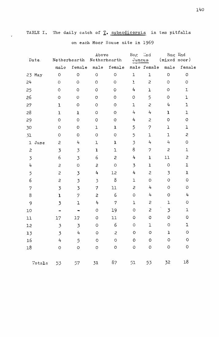
140

TABLE I. The daily catch of 1· subnodicornis in ten pitfalls

on each Moor House site in 1969

Above Bor:; :~nd Bog End Date. Netherhearth Netherhearth Juncus (mixed moor)

male female male female male female male female

23 May 0 0 0 0 l l 0 0

24 0 0 0 0 l 2 0 0

25 0 0 0 0 4 l 0 l

26 0 0 0 0 0 5 0 l

27 l 0 0 0 l 2 4 l

28 l l 0 0 4 4 l l

29 0 0 0 0 4 2 0 0

30 0 0 l l 5 7 l l

31 0 0 0 0 5 l l 2

l June 2 4 l l 3 4 4 0

2 3 3 l l 8 7 2 l

3 6 3 6 2 4 l 11 2

4 2 0 2 0 3 l 0 l

5 2 3 4 12 4 2 3 l

6 2 3 3 8 1 0 0 0

7 3 3 7 11 2 4 0 0

8 l 7 2 6 0 4 0 4

9 3 l 4 7 l 2 l 0

10 0 19 0 2 3 l

ll 17 17 0 ll 0 0 0 0

12 3 3 0 6 0 l 0 l

13 3 4 0 2 0 0 l 0

16 4 5 0 0 0 0 0 0

18 0 0 0 0 0 0 0 0

Totals 53 57 31 87 51 53 32 18

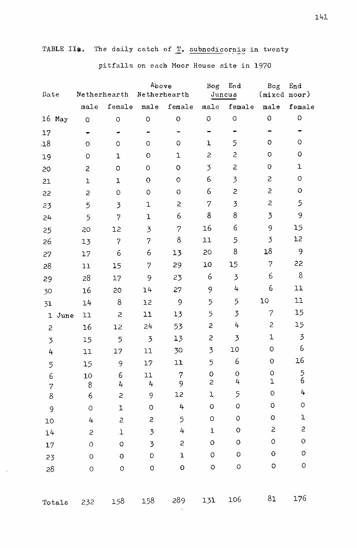
TABLE IIci.. The daily catch of_!. subnodicorni~ in tHenty

pitfalls on each Moor House site in 1970

Date Above

Netherhearth Netherhearth Bog End

Juncus Bog End

(mixed moor)

male female male female male female male female

16 May

17

0

.. 18 0

19 0

20 2

21 1

22 2

23 5

24 5

25 20

26 13

27 17

28 11

29 28

30 16

31 14

1 June 11

2 16

3 15

4 11

5 15

6 10 7 8 8 6

9 0

10 4

14 2

17 0

23 0

28 0

Totals 232

0

0

1

0

1

0

3

7

12

7

6

15

17

20

8

2

12

5

17

9

6 4

2

1

2

1

0

0

0

158

0

0

0

0

0

0

1

1

3

7

6

7

9

14

12

11

24

3 11

17

11 4

9

0

2

3

3 0

0

158

0

0

1

0

0

0

2

6

7 8

13

29

23

27

9

13

53 13

30

11

7 9

12

4

5 4

2

1

0

0

1

2

3

6

6

7

8

16

11

20

10

6

9

5

5

2

2

3

5 0 2

1

0

0

1

0

0

0

131

0

5 2

2

3

2

3

8

6

5

8

15

3 4

5

3

4

3 10

6

0 4

5 0

0

0

0

0

0

106

0

0

0

0

2

2

2

3

9

3

18

10

7

6

6

7

2

1

0

0

0 1

0

0

0

2

0

0

0

81

0

0

0

1

0

0

5

9

15

12

9

22

8

11

11

15

15

3 6

16

5 6

4

0

1

2

0

0

0

176

141

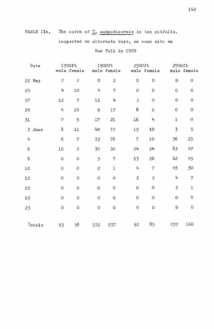
142

TABLE IIb. The catch of .!_. subnodicornis in ten pitfalls,

inspected on alternate days, on each site on

Dun Fell in 1970

Date 1700ft 1900ft 2500ft 2700ft male female male female male female male female

22 May 2 2 0 2 0 0 0 0

25 4 10 4 7 0 0 0 0

27 12 7 12 4 3 0 0 0

29 4 10 9 17 8 2 0 0

31 7 9 17 21 16 4 1 0

2 June 8 11 40 72 15 10 3 5

4 6 7 33 76 7 10 36 25

6 10 2 30 30 24 24 83 47

8 0 0 5 7 13 26 62 45

10 0 0 2 1 4 7 45 30

12 0 0 0 0 2 2 4 7

15 0 0 0 0 0 0 3 1

19 0 0 0 0 0 0 0 0

23 0 0 0 0 0 0 0 0

'l'otals 53 152 237 92 237 160

Fig. I. The accumulated pe~centage pitfall catch at each site

in 1970 plotted against date.

• Netherhearth

~ Above Netherhearth

• Bog End (Juncus)

• Bog End (mixed-moor)

A l?OOft

'V 1900ft

0 2700ft

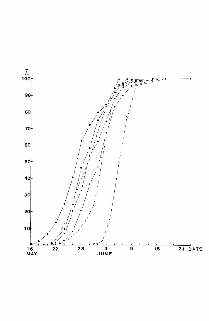
% 100

90

80

70

60

30

20

10

16 MAY

22 28 3 JUNE

9 15 21 DATE

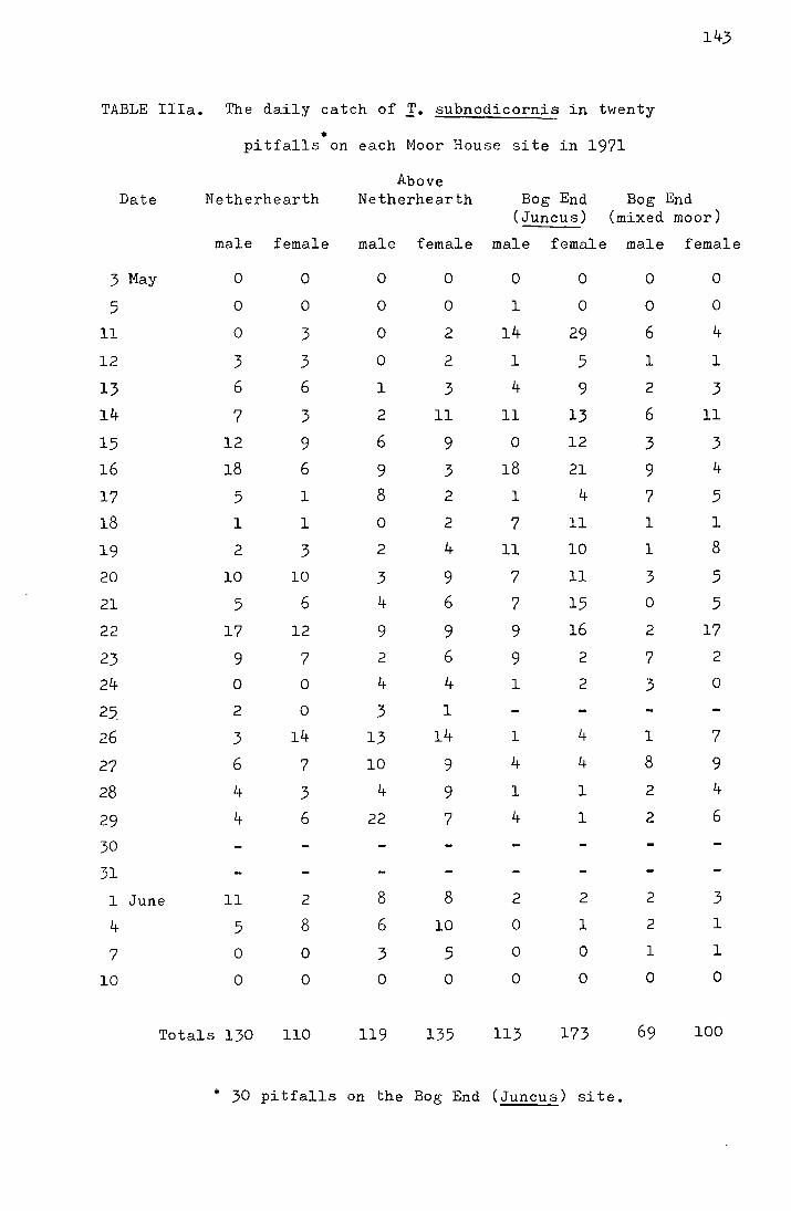
143

TABLE Ilia. The daily catch of 1'· subnodicornis in twenty

• pitfalls on each Moor House site in 1971

Above Date Netherhearth Netherhearth Bog End Bog End

(Juncus) (mixed moor)

male female male female male female male female

3 May 0 0 0 0 0 0 0 0

5 0 0 0 0 1 0 0 0

11 0 3 0 2 14 29 6 4

12 3 3 0 2 1 5 1 1

13 6 6 1 3 4 9 2 3

14 7 3 2 11 11 13 6 11

15 12 9 6 9 0 12 3 3

16 18 6 9 3 18 21 9 4

17 5 1 8 2 1 4 7 5

18 1 1 0 2 7 11 1 1

19 2 3 2 4 11 10 1 8

20 10 10 3 9 7 11 3 5

21 5 6 4 6 7 15 0 5

22 17 12 9 9 9 16 2 17

23 9 7 2 6 9 2 7 2

24 0 0 4 4 1 2 3 0

25 2 0 .3 1

26 3 14 13 14 1 4 1 7

27 6 7 10 9 4 4 8 9

28 4 3 4 9 1 1 2 4

29 4 6 22 7 4 1 2 6

30

31

1 June 11 2 8 8 2 2 2 3

4 5 8 6 10 0 1 2 1

7 0 0 3 5 0 0 1 1

10 0 0 0 0 0 0 0 0

Totals 130 110 119 135 113 173 69 100

• 30 pitfalls on the Bog End (Juncus) site.

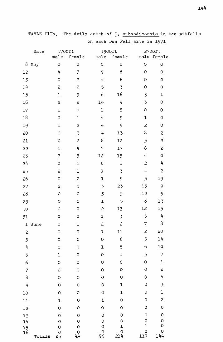
144

TABLE IIIb. The daily catch of ~· subnodicornis in ten pitfalls

on each Dun Fell site in 1971

Date 1700ft 1900ft 2700ft male female male female male female

8 May 0 0 0 0 0 0

12 4 7 9 8 0 0

13 0 2 4 6 0 0

14 2 2 5 3 0 0

15 1 9 6 16 3 l

16 2 2 ll~ 9 3 0

17 1 0 1 5 0 0

18 0 1 4 9 1 0

19 1 2 4 9 2 0

20 0 3 4 13 8 2

21 0 2 8 12 5 2

22 1 4 7 17 6 2

23 7 5 12 15 4 0

24 0 1 0 1 2 4

25 2 1 1 3 4 2

26 0 2 1 9 3 13

27 2 0 3 23 15 9

28 0 0 3 5 12 5

29 0 0 1 5 8 13

30 0 0 2 13 12 15

31 0 0 1 3 5 4

l June 0 1 2 2 7 8

2 0 0 1 11 2 20

3 0 0 0 6 5 14

4 0 0 1 5 6 10

5 l 0 0 1 3 7

6 0 0 0 0 0 1

7 0 0 0 0 0 2

8 0 0 0 0 0 4

9 0 0 0 l 0 3

10 0 0 0 1 0 1

11 1 0 1 0 0 2

12 0 0 0 0 0 0

13 0 0 0 0 0 0

14 0 0 0 0 0 0

15 0 0 0 1 1 0

16 0 0 0 0 0 0 Totals 2j 4.4. 95 214 117 144

Fig. II. The accumulated percentage pitfall catch at each

site in 1971 plotted against date

... Netherheart:b.' /j. 1700ft

... Above.Netherhearth v l900ft

• Bog End (Juncus) 0 2700ft

• Bog_ End (mixed-moor)

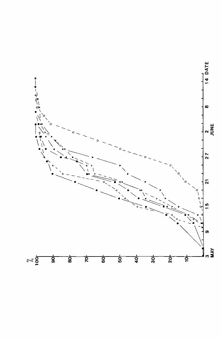
0

I e I

~\

~ 10> . \ N'o,

'

r·~~o "" "0-....... \\\ \ ~---

--0

0

" -......

0

' " 0

' " 0

' " 0

\

UJ .... < 0

~

UJ z

N;:) ...,

,.... N

~ =---~~--~~--~~---=~--~----~----~----~----~--__.Ms ......._oO 2 0 0 0 0 0 0

o-.... 0 •- CD II) ~ M N ,.... ,....

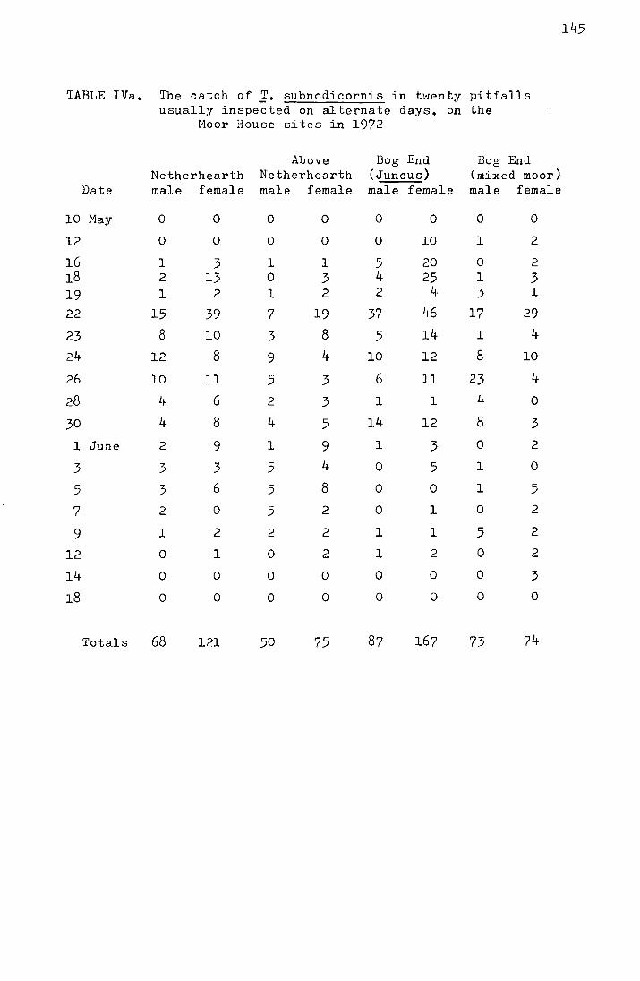
145

TABLE IVa. The catch of 1'. subnodicornis in twenty pitfalls usually inspected on alternate days, on the

Moor House sites in 1972

Above Bog End Bog End Netherhearth Netherhearth (Juncus) (mixed moor)

Date male female male female male female male female

10 May 0 0 0 0 0 0 0 0

12 0 0 0 0 0 10 l 2

16 1 3 l 1 5 20 0 2 18 2 13 0 3 4 25 l 3 19 l 2 l 2 2 4 3 1

22 15 39 7 19 37 46 17 29

23 8 10 3 8 5 14 l 4

24 12 8 9 4 10 12 8 10

26 10 ll 5 3 6 ll 23 4

28 4 6 2 3 l l 4 0

30 4 8 4 5 14 12 8 3

l June 2 9 l 9 l 3 0 2

3 3 3 5 4 0 5 l 0

5 3 6 5 8 0 0 l 5

7 2 0 5 2 0 l 0 2

9 1 2 2 2 l l 5 2

12 0 l 0 2 l 2 0 2

14 0 0 0 0 0 0 0 3

18 0 0 0 0 0 0 0 0

Totals 68 121 50 75 87 167 73 74

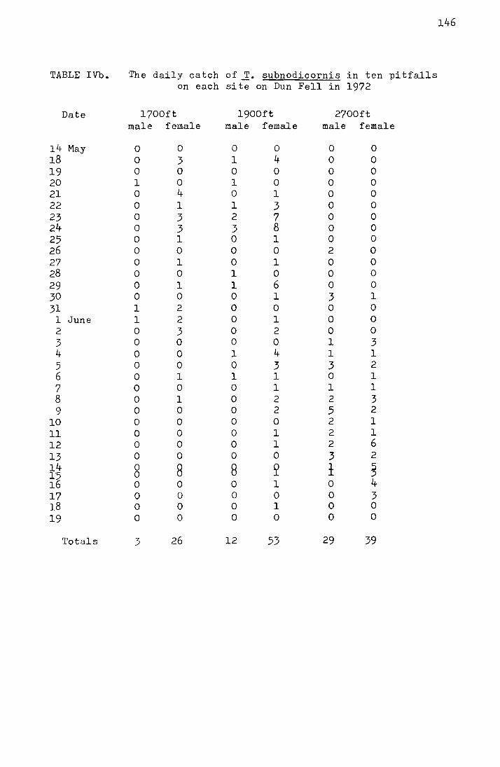
146

TABLE IVb. The daily catch of _1. subnodicornis in ten pitfalls on each site on Dun Fell in 1972

Date 1700ft 1900ft 2700ft male female male female male female

14 May 0 0 0 0 0 0 18 0 3 1 4 0 0 19 0 0 0 0 0 0 20 l 0 1 0 0 0 21 0 4 0 l 0 0 22 0 l 1 3 0 0 23 0 3 2 7 0 0 24 0 3 3 8 0 0 25 0 1 0 1 0 0 26 0 0 0 0 2 0 27 0 1 0 1 0 0 28 0 0 1 0 0 0 29 0 1 1 6 0 0 30 0 0 0 1 3 1 31 1 2 0 0 0 0

1 June 1 2 0 1 0 0 2 0 3 0 2 0 0 3 0 0 0 0 1 3 4 0 0 l 4 1 1 5 0 0 0 3 3 2 6 0 1 l l 0 l 7 0 0 0 l 1 l 8 0 1 0 2 2 3 9 0 0 0 2 5 2

10 0 0 0 0 2 l 11 0 0 0 1 2 l 12 0 0 0 1 2 6

13 0 0 0 0 3 2 14 0 8 8 2 ± ~ 15 0 16 0 0 0 1 0 4 17 0 0 0 0 0 3 18 0 0 0 1 0 0

19 0 0 0 0 0 0

Totals 3 26 12 53 29 39

Fig. III. The accumulated percentage pitfall catch at each

of the Moor House sites in 1972 plotted against date.

,• -:.

& Netherheai"th

·~ .. Above Netherhearth ..

• ·Bog hlp,d ·(Juncus)

• . Bo·g End (mi:&:ec1-moor)

-" -~

. ' .•

%

I

/

26 3 JUNE

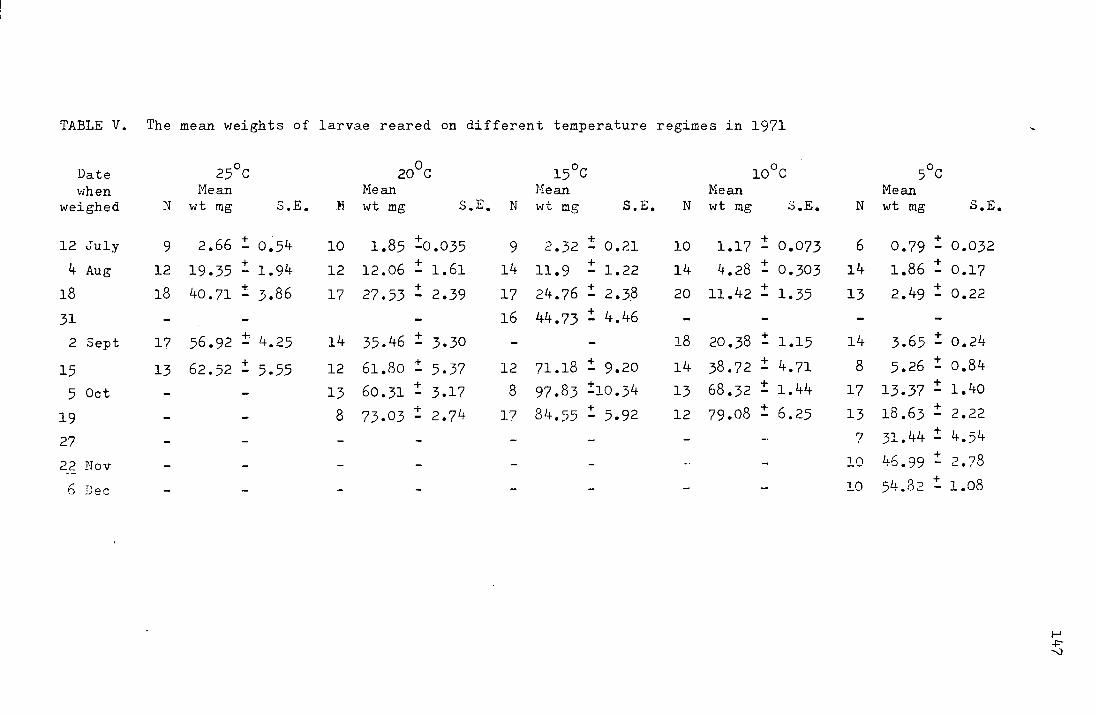
TABLE V. The mean vieights of larvae reared on different temperature regimes in 1971

Date 25°C 20°c l5°C l0°C when Mean Mean Mean Mean

weighed N wt mg s.E. . ~ wt mg s.E. N wt mg S.E. N wt mg S.E •

12 July 9 2.66 ::. 0.54 10 + 1.85 -0.035 9 +- 2 2.32 - o. l 10 + 1.17 - 0.073

4 Aug 12 + 19.35 - 1.94 12 + 12.06 - 1.61 14 11.9 + - 1.22 14 + 4.28 - 0.303

18 18 40.71 ::. 3.86 17 + 27.53 - 2.39 17 24.76 ::. 2.38 20 11.42 ! 1.35

31 - - - 16 44.73 ::. 4.46

2 Sept 17 56.92 :!; 4.25 14 35.46 :!: 3.30 - - 18 20.38 :!: 1.15

15 13 62.52 ::. 5.55 12 61.80 :!: 5.37 12 71.18 ::. 9.20 14 38.72 :!: 4.71

5 Oct - - 13 + 60.31 - 3.17 8 97.83 ::.10.34 13 68.32 :!: 1.44

19 - - 8 73.03 :!: 2.74 17 84.55 :!: 5.92 12 79.08 :!: 6.25

27 - - - - - - - -·

22 Nov - - - - - - -6 Dec - - - - - - - -

N

6

14

13

14

8

17

13

7

10

lO

5°C Mean wt mg S.E.

+ 0.79 - 0.032 + 1.86 - 0.17 + 2.49 - 0.22

3.65 :!: 0.24

5.26 :!: o.84 + 13.37 - 1.40

18.63 :!: 2.22

31.44 :!: 4.54

46.99 :!: 2.78

54.82 :!: 1.08

I-' ..j::­"'-l

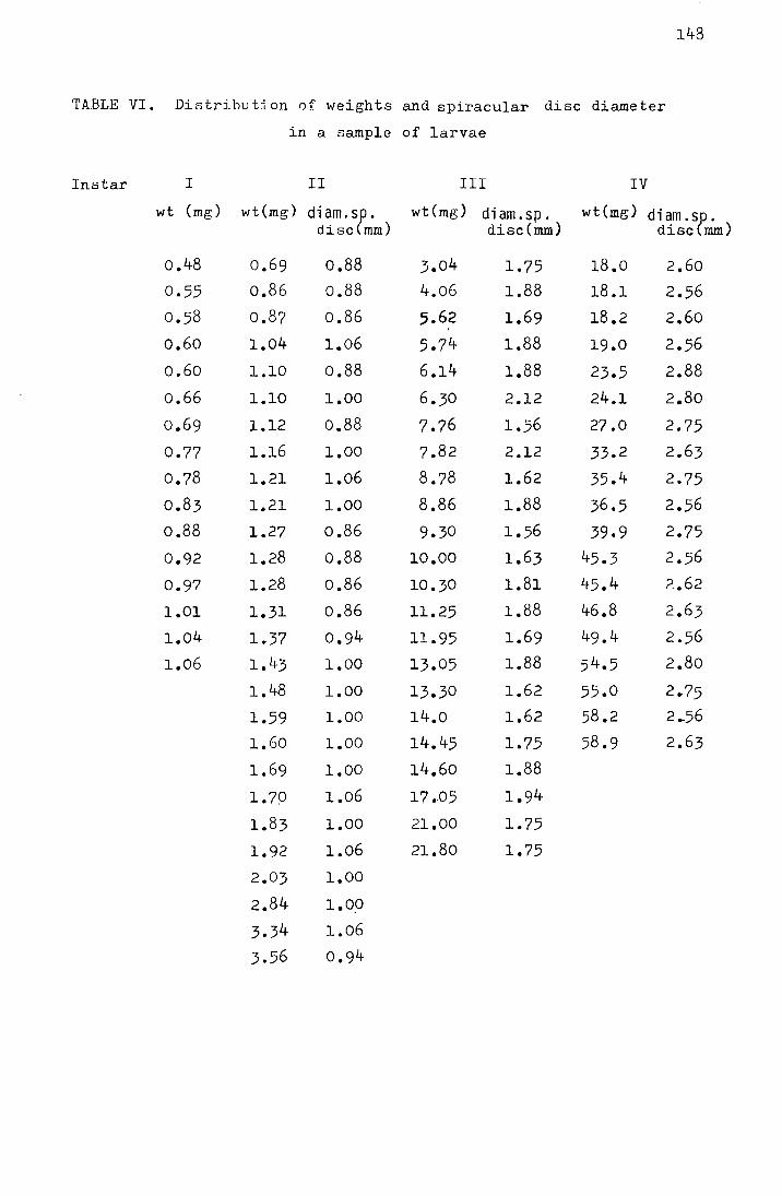
148

TABLE VI. Distribution of weights and spiracular disc diameter

in a sample of larvae

In star I II III IV

wt (mg) wt(mg) di am. s~. wt(mg) diam.sp. wt(mg) di am. s~. disc mm) disc(mm) disc mm)

o.48 0.69 0.88 3.04 1.75 18.0 2.60 0.55 o.86 0.88 4.06 1.88 18.1 2.56 0.58 o.87 o.86 5.62 1.69 18.2 2.60

o.6o 1.04 1.06 5.74 1.88 19.0 2.56 o.6o 1.10 0.88 6.14 1.88 23.5 2.88

0.66 1.10 1.00 6.30 2.12 24.1 2.80

o.69 1.12 0.88 7.76 1.56 27 .o 2.75

0.77 1.16 1.00 7.82 2.12 33.2 2.63

0.78 1.21 1.06 8.78 1.62 35.4 2.75

0.83 1.21 l.OO 8.86 1.88 36.5 2.56 o.88 1.27 0.86 9.30 1.56 39.9 2.75

0.92 1.28 0.88 10.00 1.63 45.3 2.56

0.97 1.28 0.86 10.30 1.81 45.4 ?.62

1.01 1.31 0.86 11.25 1.88 46.8 2.63

1.04 1.37 0.94 11.95 1.69 49.4 2.56

1.06 1.43 1.00 13.05 1.88 54.5 2.80

1.48 1.00 13.30 1.62 55.0 2.75

1.59 1.00 14.0 1.62 58.2 2.-56

1.60 1.00 14.45 1.75 58.9 2.63

1.69 l.OO 14.60 1.88

1.70 1.06 17.05 1.94

1.83 1.00 21.00 1.75

1.92 1.06 21.80 1.75

2.03 1.00

2.84 1.00

3.34 1.06

3.56 0.94

Fig. IV. The distribution of weights within eaoh larval instar

for a sample of 85 larvae.

. . ( .

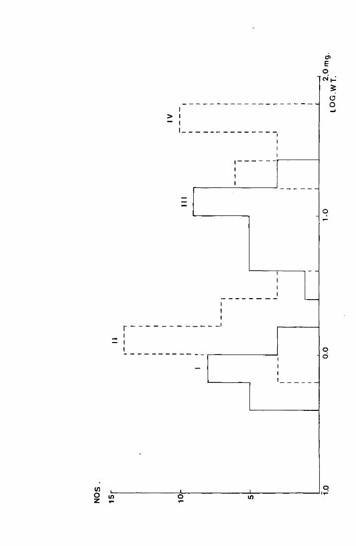
(/J

0 z

1 >I

I

--------------------! _____________ _

,-----

I

I

r-----------~ - - - - - -

..__------.------. - -

-I

r - - - - - - - - - - - -~ I I I -------------.----------....1

1 _____ _

0 ,....

q 0

~~-------------~------------L-'-----------~1~ ll) 0 ll) ,... ,...

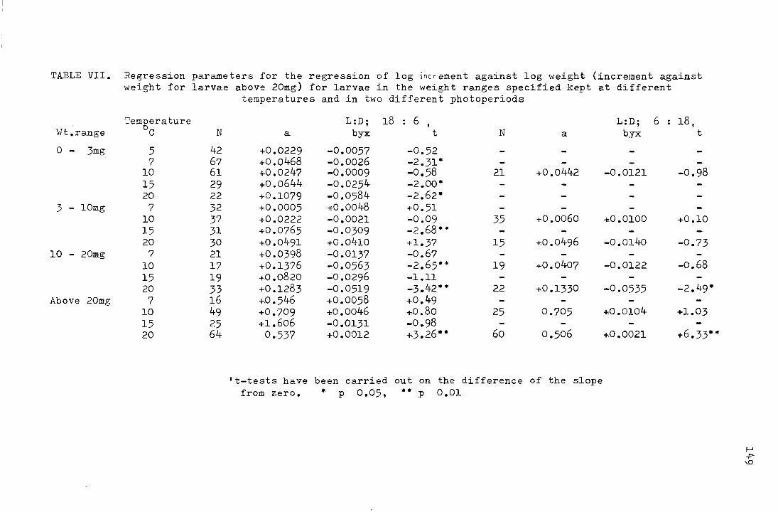
TABLE VII.

Wt.range

0 - 3mg

3 - lOmg

10 - 20mg

Above 20mg

Regression parameters for the regression of log increment against log weight (increment against weight for larvae above 20mg) for larvae in the weight ranges specified kept at different

Temgerature c N

5 42 7 67

10 61 15 29 20 22

7 32 10 37 15 31 20 30

7 21 10 17 15 19 20 33

7 16 10 49 15 25 20 64

temperatures and in two different photoperiods

L:D; 18 : 6 ' a byx t N a

+.0.0229 -0.0057 -0.52 +0.0468 -0.0026 -2.31. +0.0247 -0.0009 -0.58 21 +0.0442 +.0.0644 -0.0254 -2.oo• +0.1079 -0.0584 -2.62· +0.0005 -r.o .oo48 +0.51 +0.0222 -0.0021 -0.09 35 +0.0060 +0.0765 -0.0309 -2.68•• +0.0491 +0.0410 +1.37 15 +.0.0496 +0.0398 -0.0137 -0.67 +0.1376 -0.0563 -2.65·· 19 +.0.0407 +0.0820 -0.0296 -1.11 +0.1283 -0.0519 -:3.42• * 22 +.0.1330 +.0. 546 +0.0058 +0.49 +0.709 +0.0046 +0.80 25 0.705 +1.606 -0.0131 -0.98 0.537 +0.0012 +-3.26·· 60 0.506

't-tests have been carried out on the difference of the slope from zero. • p 0.05, ** p 0.01

L:D.; 6 : 18, byx t

-0.0121 -0.98

+-0.0100 +0.10

-0.0140 -0.73

-0.0122 -0.68

-0.0535 -2.49•

+.0.0104 +1.03

+0.0021 +6.33 ••

1-' -r=­'-0

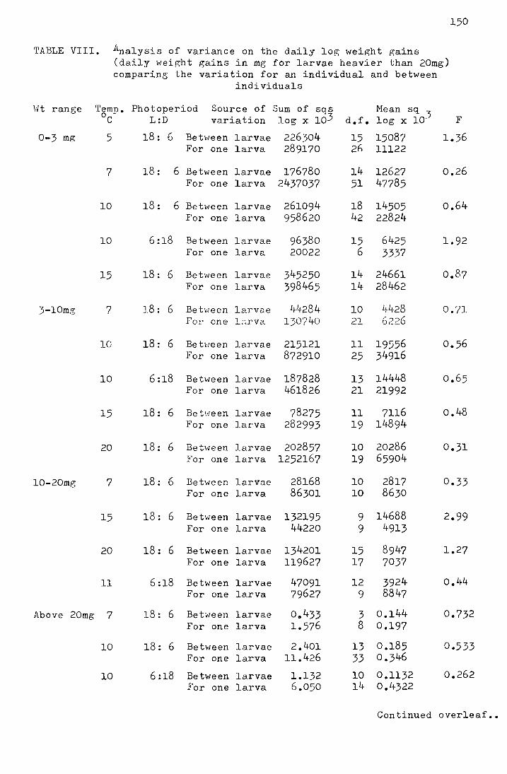
150

TABLE VIII. Analysis of variance on the daily log weight gains (daily \oJeip;h t gains in mg for larvae heavier than 20mg) comparing the variation for an individual and between

individuals

VJt range Temp. Photoperiod Source of Sum of sqs Mean sq ) oc L:D variation log x 103 d.f. log x 10- F

0-3 mg 5 18: 6 Between larvae 226304 15 15087 1.36 For one larva 289170 2h 11122

7 18: 6 Between larvae 176780 14 12627 0.26 For one larva 2437037 51 47785

10 18: 6 Between larvae 261094 18 14505 0.64 For one larva 958620 42 22824

10 6:18 Between larvae 96380 15 6425 1.92 For one larva 20022 6 3337

15 18: 6 Betv1een larvae 345250 14 24661 0.87 For one larva 398465 14 28462

3-lOmg 7 18: 6 Betv1een larvae 44284 10 4~-28 0.71 For one L'<rVa 130740 21 6226

10 18: 6 Between larvae 215121 11 19556 0.56 For one larva 872910 25 34916

10 6:18 Between larvae 187828 13 14448 0.65 For one larva 461826 21 21992

15 18: 6 Beh1een larvae 78275 11 7116 0.48 For one larva 282993 19 14894

20 18: 6 Between larvae 202857 10 20286 0.31 For one larva 1252167 19 65904

10-20mg 7 18: 6 Between larvae 28168 10 2817 0.33 For one larva 86301 10 8630

15 18: 6 Between larvae 132195 9 14688 2.99 For one larva 44220 9 4913

20 18: 6 Between larvae 134201 15 8947 1.27 For one larva 119627 17 7037

11 6:18 Between larvae 47091 12 3924 0.44 For one larva 79627 9 8847

Above 20mg 7 18: 6 Between larvae 0.,433 3 0.144 0.732 For one larva 1.576 8 0.197

10 18: 6 Between larvae 2.401 13 0.185 0.533 For one larva 11.426 33 0.346

10 6:18 Between larvae 1.132 10 0.1132 0.262 For one larva 6.050 14 0.4322

Continued overleaf ••

151

TABLE VIII. (Contd.)

Vlt range Temp Photoperiod Source of Sum of sq~ Mean sq 3 0 .

L:D variation d.f. F c log x 10 log x 10

Above 20mg 15 18: 6 Between larvae 11.237 7 1.605 1.781 (Contd.) For one larva 13.518 15 0.901

20 18: 6 Between larvae 3.129 13 0.241 1.696 For one larva 6.955 49 0.142

11 6:18 Between larvae 3.1588 13 0.2430 1.637 For one larva 6.6809 45 0.1485

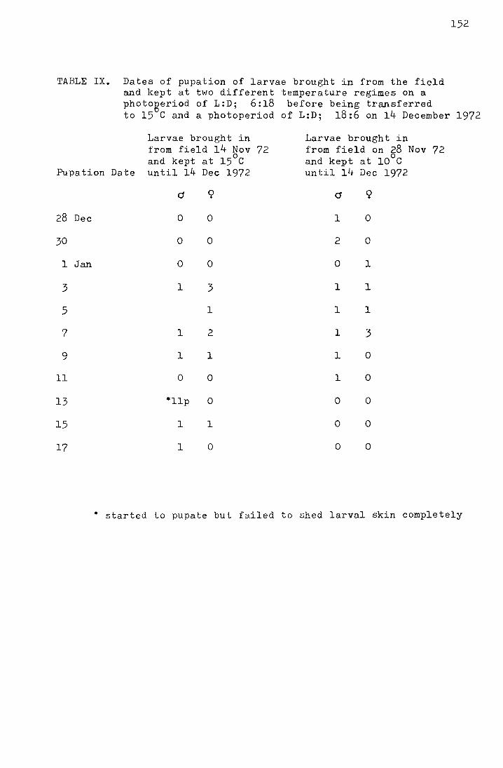
152

TABLE IX. Dates of pupation of larvae brought in from the field and kept at two different temperature regimes on a photogeriod of L:D; 6:18 before being transferred to 15 C and a photoperiod of L:D; 18:6 on 14 December 1972

Larvae brought in from field 14 Nov 72

0 and kept at 15 C

Pupation Date until 14 Dec 1972

28 Dec 0 0

30 0 0

lJan 0 0

3 1 3

5 1

7 1 2

9 1 1

11 0 0

13 0

15 1 1

17 1 0

Larvae brought in from field on 28 Nov 72

0 and kept at 10 C until 14 Dec 1972

1 0

2 0

0 1

1 1

1 1

1 3

1 0

1 0

0 0

0 0

0 0

• started to pupate but failed to shed larval skin completely

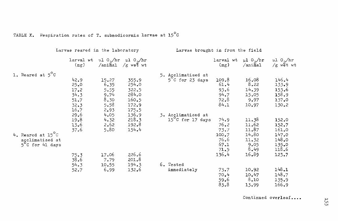
TABLE X. 0 Respiration rates of T. subnodicornis larvae at 15 C

Larvae reared in the laboratory Larvae brought in from the field

larval wt ~1 02/hr ~1 0€/hr larval wt ~1 o2/hr ~1 o2/hr (mg) /animal /g we wt (mg) /animal /g wet wt

0 5. A8climatised at 1. Reared at 5 C

42.9 15.27 355.9 5 C for 23 days 109.8 16.08 146.4 25.0 6.35 254.0 61.4 8.22 133.9 17.2 5.55 322.5 93.6 14.39 153.6 34.3 9.74 284.0 94.7 15.05 158.9 51.7 8.30 160.5 72.8 9.97 137.0 32.3 5.58 172.9 84.1 10.97 130.2 16.7 2.93 175.5 29.6 4.05 136.9 3. Acclimatised at 19.8 4.32 218.3 0

74.9 11.38 152.0 15 C for 17 days 13.6 2.62 192.8 76.2 11.62 152.7 37.6 5.80 154.4 73.7 11.87 161.0

0 100.7 14.80 147.0 4. Reared at 15 C acclimatised at 76.6 11.32 14-8 .o

0 67.1 9.05 135.0 5 C for 41 days 71.5 8.49 118.6

75.3 17.06 226.6 136.4 16.89 123.7 38.6 7.79 201.8 54.3 10.55 194.3 6. Tested 52.7 6.99 132.6 immediately 73.7 10.92 14-8.1

70.4 10.47 148.7 59.6 8.10 135.9 83.8 13.99 166.9

Continued overleaf •••• 1-' \.rJ VJ

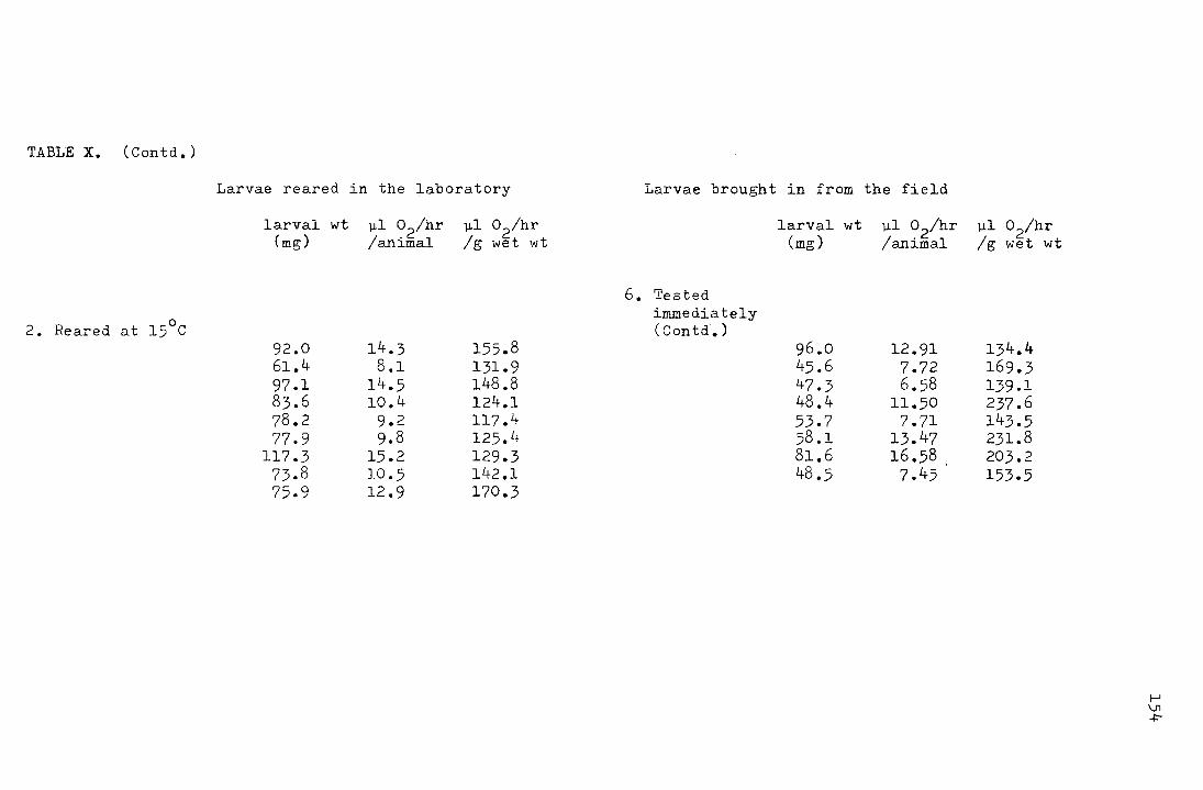
TABLE X. (Contd.)

Larvae reared in the laboratory

larval wt ].J.l o2/hr ].J.l o2/hr (mg) /animal /g wet wt

0 2. Reared at 15 C 92.0 14.3 155.8 61.4 8.1 131.9 97.1 14.5 148.8 83.6 10.4 124.1 78.2 9.2 117.4 77.9 9.8 125.4

117.3 15.2 129.3 73.8 10.5 142.1 75.9 12.9 170.3

Larvae brought in from the field

larval wt ].J.l o2/hr (mg) /animal

6. Tested immediately (Contd.)

96.0 12.91 45.6 7.72 47.3 6.58 48.4 11.50 53.7 7.71 58.1 13.47 81.6 16.58 48.5 7.45

].J.l o2/hr /g wet wt

134.4 169.3 139.1 237.6 143.5 231.8 203.2 153.5

I-' \J1 +-

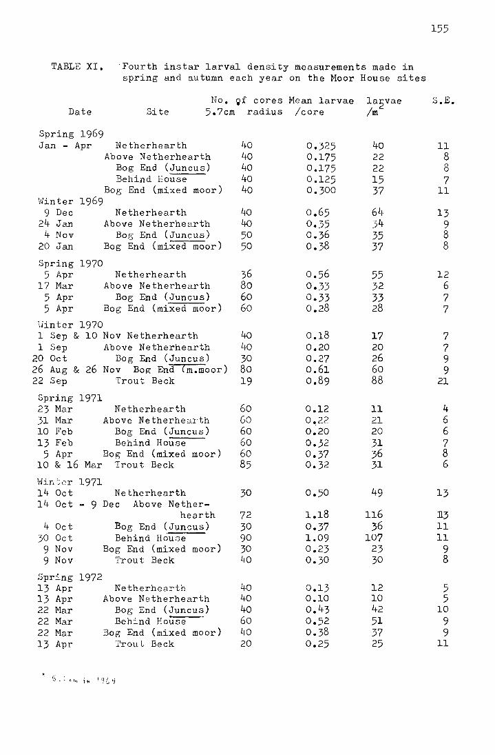
TABLE XI. Fourth instar larval density measurements made in spring and autumn each year on the Moor House sites

Date Site No. ~f cores Mean larvae

5.7cm radius /core

Spring 1969 Jan - Apr Netherhearth

Hinter 9 Dec

24 Jan 4 Nov

20 Jan

Spring 5 Apr

17 Mar 5 Apr 5 Apr

Above Netherhearth Bog End (Juncus) Behind House

Bog End (mixed moor) 1969

1970

Netherhearth Above Netherhearth

Bog End (Juncus) Bog End (mixed moor)

Netherhearth Above Netherhearth

Bog End (Juncus) Bog End (mixed moor)

\linter 1970 1 Sep & 10 Nov Netherhearth 1 Sep Above Netherhearth

20 Oct Bog End (Juncus) 26 Aug & 26 Nov Bog End (m.moor) 22 Sep Trout Beck

Spring 23 Mar 31 Mar 10 Feb 13 Feb

5 Apr 10 & 16

1971 Netherhearth

Above Netherhearth Bog End (Juncus) Behind House

Bog End (mixed moor) Mar Trout Beck

Hin'~cr 1971 14 Oct Netherhearth 14 Oct - 9 Dec Above Nether­

hearth 4 Oct

30 Oct 9 Nov 9 Nov

Spring 13 Apr 13 Apr 22 Mar 22 Mar 22 Mar 13 Apr

1972

Bog End (Juncus) Behind House

Bog End (mixed moor) Trout Beck

Netherhearth Above Netherhearth

Bog End (Juncus) Behind House

Bog End (mixed moor) Trout Beck

40 40 40 40 40

4o 4o 50 50

36 So 60 60

4o LfO

30 80 19

60 60 60 60 60 85

30

72 30 90 30 40

40 40 40 60 LfO

20

0.325 0.175 0.175 0.125 0.300

o.65 0.35 0.36 0.38

0.56 0._33 0.33 0.28

0.18 0.20 0.27 0.61 0.89

0.12 0.22 0.20 0.32 0.37 0.32

0.50

1.18 0.37 1.09 0.23 o. 30

0.13 0.10 0.43 0.52 0.38 0.25

la~vae /m

40 22 22 15 37

64 34 35 37

55 32 33 28

17 20 26 60 88

11 21 20 31 36 31

49

116 36

107 23 30

12 10 42 51 37 25

155

s.E.

11 8 8 7

11

13 9 8 8

12 6 7 7

7 7 9 9

21

4 6 6 7 8 6

13

li3 11 11

9 8

5 5

10 9 9

11

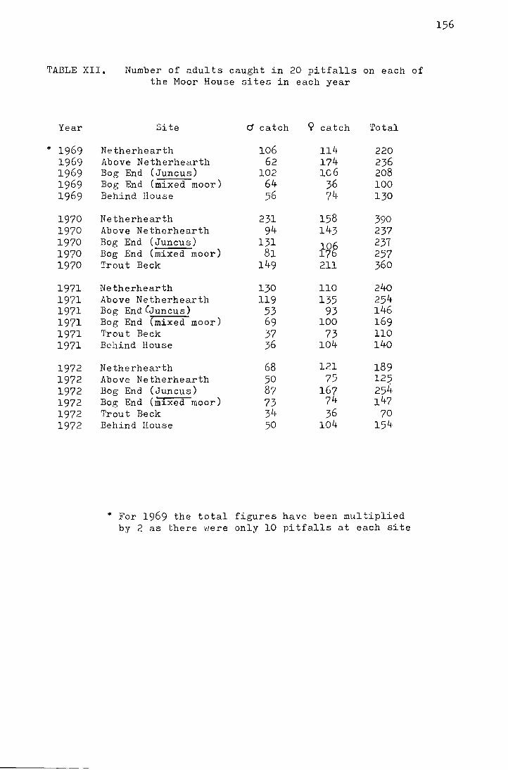
TABLE XII. Number of adults caught in 20 pitfalls on each of the Moor House sites in each year

Year

• 1969 1969 1969 1969 1969

1970 1970 1970 1970 1970

1971 1971 1971 1971 1971 1971

1972 1972 1972 1972 1972 1972

Site d catch 9 catch 'rotal

Netherhearth 106 114 220 Above Netherhearth 62 174 236 Bog End (Juncus) 102 1C6 208 Bog End (mixed moor) 64 36 100 Behind House 56 74 130

Netherhearth 231 158 390 Above Netherhearth 94 143 237 Bog End (Juncus) 131

lOg 237 Bog End (mixed moor) 81 17 257 Trout Beck 149 211 360

Netherhearth 130 110 240 Above Netherhearth 119 135 254 Bog End (Juncus) 53 93 146 Bog End (mixed moor) 69 100 169 Trout Beck 37 73 110 Behind House 36 104 140

Netherhearth 68 121 189 Above Netherhearth 50 75 125 Bog End (Juncus) 87

1*4 254

Bog End Cm1xed moor) 73 147 Trout Beck 3L~ 36 70 Behind House 50 104 154

• For 1969 the total figures have been multiplied by 2 as there were only 10 pitfalls at each site

156

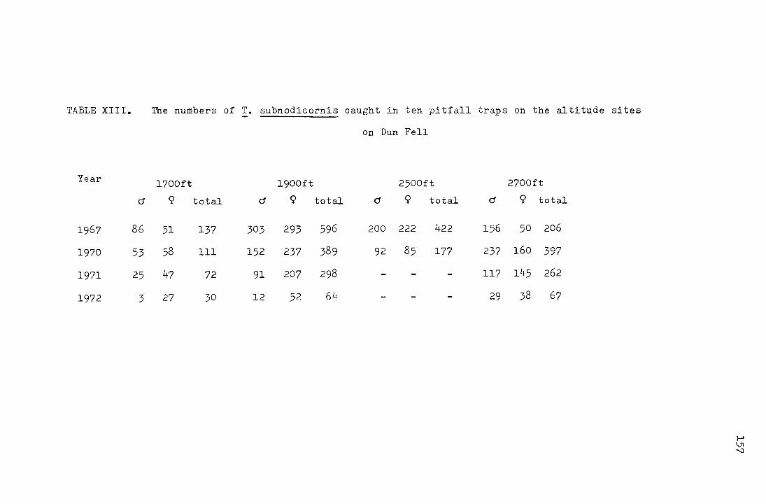
TABLE XIII.

Year

d

1967 86

1970 53

1971 25

1972 3

The numbers of T. subnodicornis caught in ten pitfall traps on the altitude sites

on Dun Fell

1700ft 1900ft 2500ft 2700ft

9 total d 9 total d 9 total Cf 9 total

51 137 303 293 596 200 222 422 156 50 206

58 111 152 237 389 92 85 177 237 160 397

47 72 91 207 298 - - - 117 145 262

27 30 12 52 6Lr - - - 29 38 67

1-' Vl -..J

Fig. V. The distribution of male and female wing lengths of

T. subnodicornis caught on the 2500ft site in 1967

plotted on normal probability papor

• male wing length (N = 199)

o female wing length (N = 222)

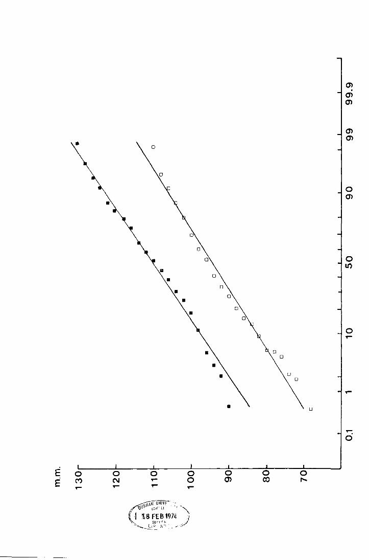
E E

•

0 M .....

•

0 N .....

0 ..... .....

0 0

0

.....

0 0>

0 U')

0 .....

.....