Durand-Kerner method for the real roots

Japan J. Indust. App!. Math., 19 (2002), 19-38 Area (2)

Durand-Kerner Method for the Real Roots

Akira TERUI and Tateaki SASAKI

Institute of Mathematics, University of Tsukuba,Tsukuba-shi, Ibaraki 305-8571, Japan

Received July 18, 1997

Revised July 21, 2000

Given a univariate real polynomial, this paper considers calculating all the real zero-pointsof the polynomial simultaneously. Among several numerical methods for calculating zero-points of a univariate polynomial, Durand-Kerner method is quite useful because it is moststable to converge to the zero-points. On the basis of Durand-Kerner method, we proposetwo methods for calculating the real zero-points of a univariate polynomial simultaneously.Convergence and error analysis of our methods are discussed. We compared our methods,the original Durand-Kerner method and Newton's method and found that 1) our methodsare more stable than Newton's method but less than the original Durand-Kerner method,and 2) they are more efficient than the original Durand-Kerner method but less thanNewton's method. We conclude that our methods are useful when good initial values ofthe zero-points are known.

Key words: Aberth's initial value, Durand-Kerner method, numerical algebraic equationsolving, polynomial real roots, Smith's error bound

1. Introduction

Given a univariate real polynomial P(x), this paper considers calculating allthe real zero-points of P(x) simultaneously.

Durand-Kerner method ([2], [5]) is widely used for calculating both the realand the complex zero-points of a univariate polynomial simultaneously. However,there are many cases in which we need only the real zero-points of a polynomial.For example, consider drawing an algebraic function on the real plane, where thealgebraic function is defined by the root of F(x, y) = 0 w.r.t. x, with F(x, y)a real bivariate polynomial. We draw a graph of the function by calculating afinite number of real zero-points of F (x, y) numerically for y = yj (j = 1, ..., k),with y l , ..., yk suitable values of y-coordinate, then connecting these zero-pointsproperly to approximate the graph of the function. In such a case, except for theneighborhood of the singular points, we have only to calculate the real zero-pointsof univariate polynomial F(x, y).

As an iterative method for calculating real zero-points of a univariate poly-nomial, Newton's method is quite popular. However, for multiple or very closezero-points, it is not easy to obtain all of these zero-points properly. On the otherhand, Durand-Kerner method is more stable hence useful than Newton's methodfor multiple or very close zero-points.

In this paper, on the basis of Durand-Kerner method, we propose two ways ofcalculating the real zero-points of a real univariate polynomial. In §2, we proposea new setting of initial values for Durand-Kerner method, which allows us to cal-

20 A. TERUi and T. SASAKI

culate the real and the complex zero-points distinguishably. In §3, we modify theiteration formula of Durand-Kerner method to calculate only the real zero-points ofa polynomial. In §4, we compare computing time of methods proposed with that ofthe original Durand-Kerner method. In §5, several numerical examples are shownto manifest efficiency, usefulness and weakness of the methods proposed.

2. DK Method and Smith's Theorem

In order to make this paper self-contained, we briefly survey Durand-Kerner

method, or DK method in short, and Smith's theorem for the error estimation.(For details, see [2], [4], [5], [6], [8], [12]).

2.1. DK iteration formula

Let P(x) be a univariate polynomial with complex coefficients.

P(x) = a°x + alx' -1 + • • • -I- an_lx + ate,, a° 0. (2.1)

In the quadratic DK method, we give numbers xl (°) , x2 (°) , ..., xn (°) initially and

calculate numbers xl ( " ) , x2(v), ... , x' ) iteratively by the formula

xj (v+l) = xj(v) —^n P((j(, — (v)) , = 1 ... n. (2.2)a0 k=1 ,^7 xj xk

Then, after some number of iterations, the numbers Xi (v) , ... , xn (L) approximate

the zero-points of P(x) quite well. The initial values xl (°) , ... , xn ( °) are usually

determined by so-called Aberth's method [1].

2.2. Smith's theoremAccurate estimation of errors of numerical results is usually quite difficult. In

the case of algebraic equation solving, however, we have the following celebratedSmith's theorem [10] which allows us to determine reasonable upper bounds of theapproximate zero-points computed numerically.

THEOREM 1 (Smith). Let xl, ... , x,,, be n distinct numbers in C andrl , ... , r, be defined as

nP(xj)rj = , j = 1,...,n. (2.3)

a0117^7

k=1,^j(xi — xk)

Let Dj (1 < j < n) be a disc of radius rj and the center at xj. Then, the unionDl U • • U Dn contains all the zero-points of P(x). Furthermore, if a union Dl U• • . U Dm (m <_ n) is connected and does not intersect with D,n+1, ... , D,, then this

union contains exactly m zero-points. q

COROLLARY 2. Let cu,. . . , ci and x l (v), ... , xn (v ) be the zero-points of P(x)

and their approximations, respectively. If every a j is a single zero-point and all the

Durand-Kerner Method for the Real Roots 21

discs defined above do not intersect with each other, then the errors of approxima-tions (") , j = 1, ... , n, are bounded as

Ix( v )P(xj(,» ( — cxi < n Uk ( — x (vi) '

j = 1, . n. 2.4 )a0 k= 1 ,O^ x^

n

The above bound is called Smith's error bound. Note that the right-hand-side of (2.4) is proportional to the "correction term" in (2.2), although the above

formula is derived independently from DK method.

2.3. Initial values for real polynomialAll the complex zero-points of a real polynomial P(x) are pairwise conjugate.

For real polynomial P(x), we can determine the initial values by modifying Aberth's

method as follows.

1. Let the zero-points be distributed within a circle of radius r and the center at

ß. Calculate ß and r°, an upper bound for r, from the coefficients of P(x).

2. Let m be the number of real zero-points of P(x), with multiple zero-points

counted as µ. Determine the value of m by Sturm's method [11].

3. Determine the initial values for real zero-points as

_ r d lx^ (°) — + r0 Ll

2j = 1, ... , m, (2.5)(m + 1 ) J '

where d 0.3.

4. Determine the initial values for imaginary zero-points as

jm—d

= ß + r° • exp n—m j =m+1, m+3,...,n-1,

(2.6)where d .: 0.3.

The number d is set to prevent the initial values to be placed symmetrically withrespect to the imaginary axis. With the above-defined initial values for DK method,

we expect that (") is real if (°) is so and = x^ (") if = x^ (°) . This

expectation is in fact true by the following proposition.

PROPOSITION 3. Let P(x), n, m and (") (j = 1, ... ,n; v = 0, 1,...) be

defined as above. Then, for v = 0, 1, 2,..., we have the followings.

1. For each j = 1, ... ,m, if (°) is real then (") is also real.

2. For each j = m + 1,m+3,. . .,n— 1, if = x^ (°) then x^+ l w> =

Proof. By mathematical induction on v. The proposition is obviously valid for

v = 0. As induction assumption, assume that the proposition is valid for 0, ... , v.

22 A. TERUI and T. SASAKI

Put P(x) = a° fl 1 (x — xk(U)) then formula (2.2) can be expressed as

x i ( v+l l = x j (vi — P(xj(v))7 ^ P,(x^ ('i)) ^

where P;(x) is the derivative of P„(x). Note that P(x) and f(x) are real polyno-mials. Therefore, if x• (') is a real number then ('+l) is also a real number becauseP(x (")) and P;(x^(')) are real, and if x +1 @') = x^(") then = x^(v+') be-cause P(x^ + l (vl) and P„(x^+l (")) are complex conjugate of P(x (")) and P„(x^(")),respectively. Hence, the proposition is valid for v + 1. q

REMARK 1. The above proposition is also valid for the cubic DK method.0

REMARK 2. We have only to calculate one of mutually conjugate roots, whichmakes the computation considerably efficient. q

REMARK 3. In the above method, Sturm's method is applied only for de-termining the number of real zero-points, not for determining the position of realzero-points. When we calculate the position of real zero-points by Sturm's method,we first calculate Sturm's sequence, then calculate the values of elements of thesequence accurately and quite many times. However, for calculating the numberof real zero-points, we have only to find the sign changes of leading coefficients ofelements of Sturm's sequence, which is quite fast. q

REMARK 4. If we set d = 0 in formulas (2.5) and (2.6), the initial values maynot converge to the true zero-points. For example, consider P (x) _ (x2 + 4) (x2 + 9)which has zero-points at x = ±2i and x = ±3i, and define the initial values asx1^°^ = a + bi, X2 (°) = xl (°) , x3 0) = -1 °) and x4^°) = —x1(0) , where a, b E R.Then, formula (2.2) gives us x 2 w> = xl('), x3 01) _ —xlw) and x4 (") = —x 1 (") forv = 1, 2, ..., hence some of x^ ( L ) will never converge to the corresponding zero-points.

Note that, even if we set as d 0.3, DK method may not give a sequenceof numbers which converges to the zero-points. Therefore, we must be careful todefine the initial values for DK method so that they converge correctly. q

Throughout this paper, we call DK method with the above-determined initialvalues "DKAreal," while we call DK method with Aberth's initial values "DKA."

3. DK Method Calculating Only Real Roots

In this section, assuming that P(x) is monic and that all the coefficients ofP(x) are real, we make a modification of DK method so that we will calculate onlythe real zero-points of P(x).

Let F(x) and G(x) be polynomials and assume that the degree of F(x) isgreater than or equal to that of G(x). Throughout this paper, we denote polynomialquotient of F(x) divided by G(x) by quotient(F(x), G(x)).


3.1. Modification of DK formula

We first state how we modify DK method.

1. Let the roots be distributed within a circle of radius r and the center at ß.

Calculate ß and ro, an upper bound for r, from the coefficients of P(x). Note

that ß is real.

2. Let m be the number of real zero-points of P(x), with ,a multiple zero-points

counted as p. Determine the value of m by Sturm's method.

3. Determine the initial values for real zero-points as

xj (o) =ß+ro L l — 2(m + d) J j = 1,...,m, (3.1)

where d. 0.3.

4. Modify DK iteration formula as

x .(v+l) j=1= x.(v) — P`xj(v)) ... m,7

rk=1 j (xi (v) — xk(v)) . Qv(xj (v))(3.2)

where

Qv(x) = quotient (P(x), fk 1 (x — xk ( v ) )) . (3.3)

Obviously the calculated values X I (V

) , x2(ß), ..., xn ( v ) are real numbers for all

v. Throughout this paper, we call the above method "DKreal."

3.2. Convergence propertyLet al, ... , a,, be the zero-points of P(x), where we assume that the real zero-

points are al, ... , am (m < n) and P(x) is monic, for simplicity. Assume that

a l = ... = a,n, (m' < m) and ak 0 a l for k >_ m' + 1. Let xl ( v ) , ... , xm, ( v ) be

the approximations of a1, . .. , am , respectively. Put ej ( v ) = xj (v ) — aj and assume

that Iej ( v ) I K 1 for j = 1, ... , m. Then, formula (3.2) allows us to calculate ej (v+ 1 )

(1 <j < m') as follows.

E.j (v+l) = xj(v+l) — aj

= x j(v) —H

( P(x^ (v))

k= 1 ,54j`x^ (v) — xk(v)) . Q,(xj(v))

—a .7

_ Ej(v) — m, (E^ (v) )m m x^(v) — ak ][ rlk=I, :„^j(Xj (v) — xk (v) )

k=m +1 x^(v) — xk(v)

llk=m+1(xj(v) — Cek)1(3.4 )X II

Qv(xj( ))

Let

so(v) = max{ I El(v) i, ... , ISm (v) I (3.5)


then we see

m xj(v) - ak m Ek(U)k- 1 xj ^ u) - xk(') k- 1 ^l + xj(

v) - xk( v) )

=

1111

6k^

k=m'+1

(i+al+e (V) - xk(V))

= Ek(v)1 1 11 (+ ^v) + O(Ej (v) Ek (L) ))

k=m.'+1 al - xk

m

= 1 + (U) + O((so (u ) ) 2 ). (3.6)k=m,+1 al - ^k

We next consider the quotient Q„(x). Dividend in the right-hand-side of (3.3) is

decomposed as follows.

m nP(x) _ JJ(x - Xk (V) + Ek (U)) 11 (x - ak)

k=l k=m+1

_ fl (x - xk (v) ) 11 (x - ak) + Z [ @' 11 (x - ak) J( + O(2(x))

k=1 k=m+1 j=1 k=1,ßj m n

_ [f (x-xk^v)) 11 (x-ak)k=l k=m+1

+ Z [ex - x + x -an) 11 (x -ak) 1 + O(r2(x))j- 1 k=l, j

m n

_ H(x-xkv) ) 11 (x-ak)k=1 k=m+1

m ( m n-1 n-1+ ^E^v) ` 11(x - x) (x - ak) + (x^L) - an ) (x - ak)j1 I\k=1 k=m+1 k=1,ßj

+ O(e 2 (x)), (3.7)

where O(e2 (x)) denotes a polynomial of terms whose coefficients are of magnitudes

O((eov) ) 2). Continuing this rewriting, we see

Qv(x) = l lk=m+1 (x - ak) + äQv (x), (3.8)

where

in n-1 n-2

öQV(x) = Z Env) ( 11 (x - ak) + (x^v) -an) 11 (x ak) + ... + O(^ 2 (x))j=1 Illl k=m+l k=m+1

(3.9)


Remembering that x(v) = al + O(e (v) ), j = 1, ... , m, we find

SQ,(xj ( v ) ) = 6Q7(al) + o((Eo ( v) ) 2 ), 6Q71(a1) = O(xo (v ) ), (3.10)

and we obtain

llk=m+1 (x 71) ak) _ l lk=m Fl (x (v) - ak)

Q7(x (v) ) l Ikn (xjv) - ak) + SQv(x(v) )=m+1 j

— 1— 7-^ aQv((x' (v)) + O((eo (v) ) 2 )11k=m+l lxj (v) - ak)

= 1— 7-^ JQU(al)+O((eo(v))2). (3.11)11k=m+1(al - ak)

In the case that a 1 is a single zero-point, i.e. m' = 1, the above argumentslead us to the following.

el (v+l) = el (v) — sl (' ) . (1 + O(eo(V)))(1 + O(eo (v) )) = O(el (') so ( v) ). (3.12)

PROPOSITION 4. Let a1,. . . , a m be the real zero-points of P(x) and assume

that aZ aj for any i j. Let xl ( v ) ... x,,, (v) be the approximations ofa1,. . . , a,m , respectively, and assume that every xj (v) is sufficiently close to a.Then, iteration formula (3.2) converges quadratically. q

If m' > 2, the approximations x1(ß), ... , x , ( v) corresponding to m' multipleroots do not converge quadratically. However, we find that the "center" of theseapproximations, or (x1 (71) + • • • + Xm' (v))/m', converges quadratically, as we willshow below.

PROPOSITION 5. Let a1,. . . , am be the real zero-points of P(x) and assumethat a1 = • • • = am, (m' < m) and al az aj for m' < i < j <_ m. Let

Lbe the approximations of a xl( ) ^...^xm^ Opp f 1 > ...‚ am', respectively, and assumethat every xj ( V ) is sufficiently close to aj. Then, (x1 (71) +• • •+xm' ( v) )/m' converges

to a 1 quadratically.

Proof. Using (3.4), we can calculate the error of the "center" as follows.

I m'

j=1

m' / (v))m 11 /^j(v) _[ m '

(Ei

m '_1 { rlk=1 (xj (v) -xk() )

Xm xj(v) - akllk=m+1(xj(v) - (kk)

yk=m

;+1

xj (v) - xk(v)Q,(xj(v))


m' m ( (v) )m'

= E^(v) — -' m (E7

m3=1 jL=1 llk=l,^j(Ej(v) --k(v))

m ^k(v)

X 1 + + O((Ep(v) ) 2 )

k=m'+1 ala— x/('')

r SQ_(al) (( (v ) )z) 1X L 1 — ^k=m+1(al — ak) + O

EpJ}

ii

v (r(i))m' -

:im, j= 1 j=1 llk=l, ^j (ei (v) — Ek(v)) j=1 [ Ilk=l„4j(Ej(v) — -k(v))

m 'k(v)_ 7--^ ÖQ (al) 1 .

v

X Lmr+1 a1 — Xk (v) l lk=m+1 (al — ak) + O

(( Ep

()

)z

)

(3.13)

In the right-hand-side of (3.13), we have

m' (E („)) m'

m ' i(v)• (3 . 14 )

j=1^7 v vllk /1,#jj ( ) — fik ( )) — ^

s 3.14

This can be seen as follows. Putting

rT ^7 (U) (v_ ^ (v))m' llj =11 l lk j, '+1(Ej — Ek

) )

F

(

j=1 1 11k=1,ßj (6j (v) — Ek (v) )

m'-1 m'

= 11 11 (ei»" ) — sk ( v ) )j'=1 k=j'+1

Wr4& Q I

m (Ej(v))m F

mr v vrk= 1

, j(^j( ) — Ek( )) G

We note that F and G are polynomials in Ej (v) (j = 1, ... , m'). If we put e1(' =Ez (,) then we see G = 0 directly and we find F = 0 because the first and the secondterms in the summation over j cancel each other and other terms become zero.Similarly, for any i # j, if we put ei ( r' ) = ej(v) then we obtain F = G = 0. Thismeans that every factor in G is contained in F, therefore we find GIF. PuttingH = F/G, we see from F and G that H is a symmetric polynomial. With respect toany "variable" env) , 1 < j < m', the degree of H is 1, H contains no constant termand the leading coefficient of H is 1 because those of F and G are 1. Therefore, His an elementary symmetric polynomial of degree 1, which is s1 (" ) + • • • + e*'.


Equation (3.14) allows us to rewrite (3.13) as follows.

/ m Ej (v+1)

1 (e^(v))m

' III,m #^ ((^ (v) — Ek (U) )m n

X al^k(xk(v) rlk= }1(Ckl^ CYk) +O((eo(v))2)k=m'+1

= O((eo (v ) ) 2 ). (3.15)

Therefore, the "center" of x l ("), ... , x(') converges to al quadratically. q

A property described in Proposition 5 is called "quadratic-like convergence ofthe mean." We note that this property is discussed by Fraigniaud [3] and Iri [4] forDurand-Kerner method and by Pasquini and Trigiante [7] for its variations.

3.3. Error boundWe can estimate an upper bound of the errors of the approximations

• . ,x,,,( ) , by the following proposition.

PROPOSITION 6. Let P(x), ak (k = 1, ... , n) and (") (j = 1, ..., m) bedefined as above. Let r be defined as

P(x ( U>)

r' = n m (3.16) (v) / (v)' j _ ... >

a— xk )'Qvlx^ )

and D (1 < j < rn) be a disc of radius r and center at ( v ) . Then, the errors ofapproximations x^ (v), j = 1, ... , m, are bounded as

x^(v) — a' r'' 1 — 6Q, (x^ v ) j = 1, ... m, (3.17)

if all the discs D^, j = 1, ... , m, do not intersect with each other and each x^ ( v ) issufficiently close to c.

Proof. Applying Theorem 1 to the case that xj = xj (v) (j = 1, ... , m) andXk = ak (k = m + 1, ... , n), we have

P(x^(v))r^ = n ao fk

i>(x^ (v) — xk (v) ) . Uk=m+i(xj(v) — ak)

Using (3.8), we rewrite the above expression as

P(x(')) ( )

r^ — n ao Hk i,^ (xj (v) — xk (v) ) . {Qv(x^ (v) ) — 5Qv(x^(v))}3.18


Since xj (v) is sufficiently close to aj , we have

Q,(xj ( V ) )I » 1JQv(xj ( v ) )1= 0(EO ( v ) )

Therefore, we have

-IP(xj (v) ) 8Qv(xj(v))

r ^ — n ao flr i,^ (x^ (v) — xk(V)) Qv(x ) 1 Qv(x^ (v) )( v) -1

= Ti'1 — SQv(xj )

(3.19)7 Qv(xj(v))1 q

REMARK 5. We can estimate the number I1 — ÖQv (xj (v))/Qv (xj(U))^ —I informula (3.19) as

1 — 5Qv(xj (U) ) — - 1 + I8Qv(xj(v))I (3.20)

Q, (xj (v) ) 1Q,(xj(v))I

Therefore, the errors of x (v), j = 1, ... , m, are approximately bounded as

1xj (v) -aj 1 <r \1+ I SQv(xj(v )^ I / j

= 1,...,m. (3.21)Qv(xj (v)

U

REMARK 6. We can estimate the number in formula(3.19) quite precisely as follows. Formula (3.8) tells us that

Q,(xj (v) ) — Q,.+I(xj °' ) ) = JQv (x^ ( v ) ) — 8Qv+i (xj ( v ) )

JQv(xj (v) ),

because I SQv+l (x j (")) I « I8Qv (x j (v)) I . Therefore, we have

SQv(xj ( v ) ) ^_ IQ,(xj(U))-Qv+I(xj(v))I (3.22)

Q, (xj (v) ) I Qv(xj (v) )I

W

4. Computing Time Analysis

Let P(x) be a monic polynomial of degree n and let m be the number of realzero-points of P(x), as above. In this section, we analyze the computing time forone iteration in algorithms DKA, DKAreal and DKreal. Here, by "computingtime" we mean the number of arithmetic operations (addition, multiplication anddivision) on real numbers, because the ordinary CPU executes only real arithmeticoperations. For operations on polynomials, we consider only the number of coef-ficient operations and discard the operations on structuring polynomials such assorting and collecting terms.


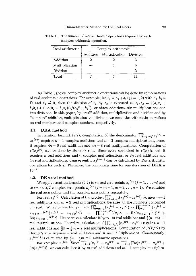
Table 1. The number of real arithmetic operations required for each

complex arithmetic operation.

Real arithmetic I Complex arithmetic

Addition Multiplication Division

Addition 2 2 3

Multiplication — 4 6

Division — — 2

Total 1 2 6 11

As Table 1 shows, complex arithmetic operations can be done by combinationsof real arithmetic operations. For example, let z j = a + bi (j = 1, 2) with a^, b E

R and z2 # 0, then the division of zl by z2 is executed as zl/z2 = {(ala2 +

ó1b2) + (—a l b2 + bla2)i}/(a2 2 — b2 2 ), or three additions, six multiplications andtwo divisions. In this paper, by "real" addition, multiplication and division and by"complex" addition, multiplication and division, we mean the arithmetic operationson real numbers and complex numbers, respectively.

4.1. DKA methodIn iteration formula (2.2), computation of the denominator JJ(xj ( v ) —

Xk ( ')) requires n — 1 complex additions and n — 2 complex multiplications, henceit requires 4n — 6 real additions and 4n — 8 real multiplications. Computation ofP(x^(v)) can be done by Horner's rule. Since every coefficient in P(x) is real, itrequires n real additions and n complex multiplications, or 3n real additions and4n real multiplications. Consequently, x can be calculated by 15n arithmeticoperations for each j. Therefore, the computing time for one iteration of DKA is15n2 .

4.2. DKAreal methodWe apply iteration formula (2.2) to m real zero-points ( v ) (j = 1, ... , m) and

to (n — m)/2 complex zero-points (") (j = m + 1, m + 3, ... , n — 1). We considerthe real zero-points and the complex zero-points separately.

For real xj ("): Calculation of the product f k 1 #i (xi ( v) —xk(v ) ) requires m-1real additions and m — 2 real multiplications, because all the numbers concernedare real. We calculate the product f k_m+1 (xi ( " ) — xk(U ) ) as fl(nl m)/2 (x^(v) —

(v))(x (v) — xm (,,)) _ Ij (n—m)/2 [{x (v) — Re(xm+21- 1 (v))} 2xm +F21-1 j ^2l l=1

Im(xm+21_1 ()) ) 2]. Hence we can calculate it by n—m real additions and 2 (n—m)-1

real multiplications. Therefore, calculation of ^k=1 o^ (xi ) — xk ( v ) ) requires n —1

real additions and 2 n — 2 m — 2 real multiplications. Computation of P(x (")) byHorner's rule requires n real additions and n real multiplications. Consequently,x^(U+1) is calculated by 2n — Zm real arithmetic operations.

For complex xj ( v ) : Since flk 1 (xß ( v ) — xk(v ) ) =flk 1 {Re(xí ( v)) — xk ( v ) +Im(x (" ) )i}, we can calculate it by m real additions and m — 1 complex multiplica-


tions, or by 3m — 2 real additions and 4(m — 1) real multiplications. We calculatethe product rjk=m+1 , ^ (x^ ( v ) —xk(v)) by n—m-1 complex additions and n—m-2complex multiplications, or 4(n — m) — 6 real additions and 4(n — m — 2) real mul

-tiplications. Computation of P(xj (')) is executed by Horner's rule with the samecomputing time as in DKA. Therefore, x^ (+1) is calculated by 15n — m — 1 realarithmetic operations.

Consequently, the computing time for one iteration in DKAreal is

m^9n-2m)+( n 2 m )(15n—m)= ßn2 —2mn. (4.1)

We see that, if the number of real zero-points is small, the computing time ofDKAreal is approximately equal to the half of that of DKA, and it decreases asm increases.

4.3. DKreal methodIn DKreal, all the computations are done with real arithmetic. In each it-

eration step of (3.2), we calculate Q(x) in (3.3). Since the multiplication of twomonic polynomials of degrees k and 1 requires k —1 additions and k —1 multiplica-tions on their coefficients, calculation of a term Il' 1 (x — xk(v)) requires m2 — marithmetic operations. Next, we consider the quotient (P (x) 7 rIkm= I (x — xk(vl)).Let F(x) = aox'' + alxn — ' + • • • + a_ix + a. and G(x) = f 1 (x — xk ( ' ) ) =xm + blxm-1 + • • • + b_ l x + bm . The elimination of the leading term of F(x) byG(x) is executed as F(x) — aoxn —mG(x) and it takes 2m arithmetic operations (mmultiplications for calculating the coefficients of aoxn — mG(x) and m additions forcalculating the coefficients of F(x) — aoxn — mG(x)). Since the polynomial divisionof P(x) by G(x) requires n — m +1 eliminations of the leading term, calculation ofthe quotient(P(x), f k 1 (x — xk("))) requires 2m(n — m+ 1) arithmetic operations.Therefore, the computing time for Q„ (x) is 2mn — m2 + m.

In iteration formula (3.2) for DKreal, the denominator 11 7n 1 (x^ (v) — xk ( ) )

requires m — 1 additions and m — 2 multiplications. Evaluations of P(x(')) andQ,(x^ (' ) ) require 2n and 2(n — m) arithmetic operations, respectively. Conse-quently, x ('+') can be calculated by 4n — 1 arithmetic operations for each j.Therefore, the computing time for one iteration in DKreal is 6mn — m 2 .

We see that, if the number of real zero-points is small, the computing time ofDKreal is approximately equal to 5m/n of that of DKA. However, as the numberof real zero-points increases, the computing time of DKreal increases in proportiontorn.

5. Experiments

We have implemented the algorithms DKA, DKAreal and DKreal onGAL [9] (General Algebraic Language/Laboratory, a LISP-based general purposecomputer algebra system), using numeric computation functions in LISP and GAL'sfacility of computing polynomial quotient. All the following experiments were car-ried out on a SPARC Station 5 (microSPARC II of 85 MHz) with 32MB RAM.


The computing time is shown in milli-seconds and the time for garbage collectionis discarded.

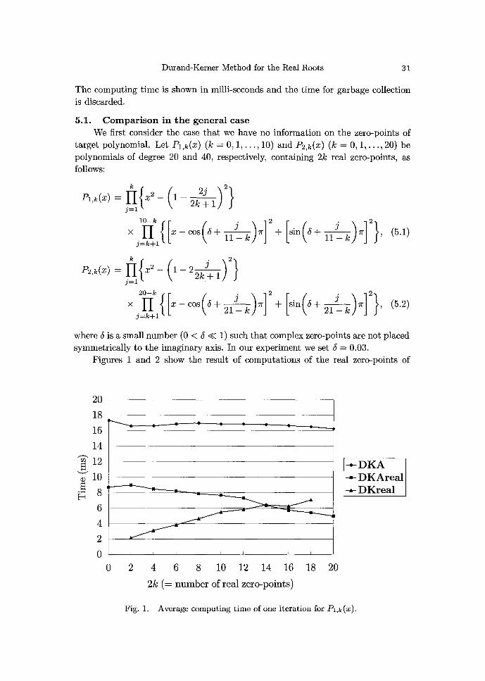
5.1. Comparison in the general caseWe first consider the case that we have no information on the zero-points of

target polynomial. Let P1,k(x) (k = 0, 1, ...,10) and P2 ,k(x) (k = 0,1, ..., 20) bepolynomials of degree 20 and 40, respectively, containing 2k real zero-points, asfollows:

k ) 2 }(/

P1 ,k(x) _1{ x2 —I 1-2k

2j

+ 1

x 111 { [x — cos (S + 11

k ) ]^r] Z + [sin (S + 113 k )7r 1 2 1 , (5.1)

j l /

2

PZ ,k(x) = 1

x2 — 3(1-21)

j=

x 20-k X —cos( + 21i k)ß]2+ [sin(ö+ 21

i k)W]Z}, (5.2)k +1 \ J

where S is a small number (0 < ó « 1) such that complex zero-points are not placedsymmetrically to the imaginary axis. In our experiment we set 6 = 0.03.

Figures 1 and 2 show the result of computations of the real zero-points of

20

18

16

14

12

9 10

Ei 8

6

4

2

0

DKA-F DKAreal-r DKreal

0 2 4 6 8 10 12 14 16 18 20

2k (= number of real zero-points)

Fig. 1. Average computing time of one iteration for Pl,k(x).


80

70

60

50

40

E30

20

10

0

-.-DKA{ DKAreal-r DKreal

0 4 8 12 16 20 24 28 32 36 40

2k (= number of real zero-points)

Fig. 2. Average computing time of one iteration for P2,k(x).

Pi , k(x) and P2,k(x), respectively. We measured the computing time by repeatingeach computation 10 times and calculating the average for one iteration.

We see that computing time of one iteration of DKAreal is approximatelyequal to the one-half of that of DKA for k = 0, and it becomes smaller as kincreases. We also see that computing time of one iteration of DKreal increasesas k increases, and it becomes greater than that of DKAreal for relatively largevalue of k.

5.2. Usefulness in a special caseWe next consider the case that we know rather good approximations of real

zero-points of target polynomial. Such a case happens quite often practically. Forexample, let us consider drawing an algebraic function on the real plane, determinedas the solution of a bivariate polynomial equation P3(x, y) = 0. Let P3(x, y) be asfollows. t

P3(x, y)

= 93392896/15625x6 + (94359552/625y 2 + 91521024/625y — 249088/125)x 4

+ (1032192/25y4 — 36864y3 — 7732224/25y2 — 207360y + 770048/25)x2

+ (65536y6 + 49152y5 — 135168y4 — 72704y3 + 101376y2 + 27648y — 27648).

(5.3)

Throughout this paper, by deg x (P3(x, y)) we denote the degree of P3(x, y) withrespect to x. Function P3 (x, y) = 0 has eight multiple points of multiplicity 2 in


the real plane; two are on lines which are tangent with horizontal line y = \, twoare "cusps" at (0, —1) and (0, 3/4), and the other four are isolated points at

—380/351 ( —1.0997150997151),

y —41/76 (-- —0.53947368421053).(5.4)

Suppose we draw the graph in the interval —1 < y < ^. We first divide the y-axisof drawing area into the following three intervals.

Il = [-1.0, —0.53947368421053 1 ,

12 = [-0.53947368421053, 0.75], (5.5)

13 = [0.75, 1.414213562] .

In each interval I^ (1 < j < 3), we calculate the graph of P3(x, y) = 0 on the realplane as follows.

1. Let y^,o = (max I3 + min I^ )/2 (the middle point of Ij ) and Sj = (max I3 —min I)/L, where L is an even integer such as L -- 10, and divide Ij into Lsubintervals of width ö3.

2. Calculate the zero-points of univariate polynomial P3(x, y^, o ).

3. Let Yj,±k = yj ,o ± kör (k = 1, ... , L/2 — 1) and calculate the, zero-points ofpolynomials P3(x, Yj,+k) and P3(x, yj,_k), respectively. In order to calculatethe zero-points of P3(x, yj,±(k+ll), use the zero-points of P3(x, yj,+k) as theinitial values.

4. Connect the real zero-points computed smoothly.

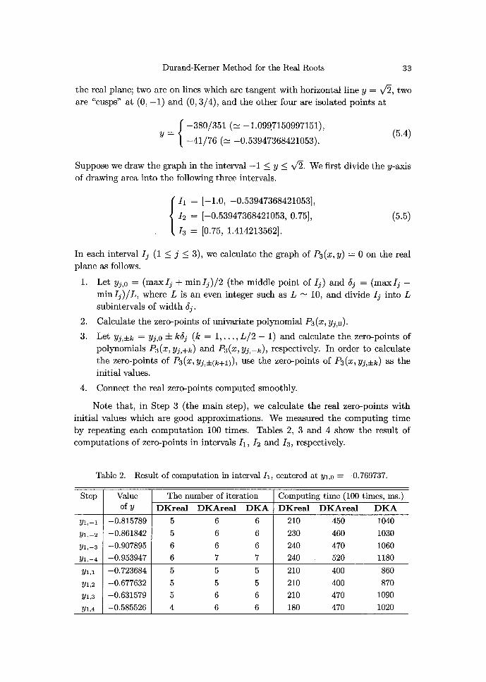
Note that, in Step 3 (the main step), we calculate the real zero-points withinitial values which are good approximations. We measured the computing timeby repeating each computation 100 times. Tables 2, 3 and 4 show the result ofcomputations of zero-points in intervals Il , 12 and 13, respectively.

Table 2. Result of computation in interval Il, centered at yl,o = —0.769737.

Step Value The number of iteration Computing time (100 times, ms.)of Y DKreal DKAreal DKA DKreal DKAreal DKA

—0.815789 5 6 6 210 450 1040

y 1 ,_ 2 —0.861842 5 6 6 230 460 1030

y1,_3 —0.907895 6 6 6 240 470 1060

y1,_4 —0.953947 6 7 7 240 520 1180

y1,1 —0.723684 5 5 5 210 400 860

y1,2 —0.677632 5 5 5 210 400 870

y1,3 —0.631579 5 6 6 210 470 1090

y1,4 —0.585526 4 6 6 180 470 1020


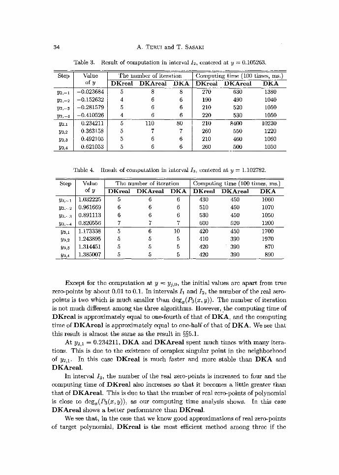
Table 3. Result of computation in interval 12, centered at y = 0.105263.

Step Value The number of iteration Computing time (100 times, ms.)of y DKreal DKAreal DKA DKreal DKAreal DKA

y2,-1 -0.023684 5 8 8 270 630 1380

y2,-2 -0.152632 4 6 6 190 490 1040

y2,-3 -0.281579 5 6 6 210 520 1050

y2,-4 -0.410526 4 6 6 220 530 1050

y2,i 0.234211 5 110 80 210 8400 10230

Y2,2 0.363158 5 7 7 260 550 1220

y2,3 0.492105 5 6 6 210 460 1060

y2,4 0.621053 5 6 6 260 500 1050

Table 4. Result of computation in interval 13, centered at y = 1.102782.

Step Value The number of iteration Computing time (100 times, ms.)of y DKreal DKAreal DKA DKreal DKAreal DKA

P3,_1 1.032225 5 6 6 430 450 1060

Y3,-2 0.961669 6 6 6 510 450 1070

y3,-3 0.891113 6 6 6 530 450 1050

y3,-4 0.820556 7 7 7 600 520 1200

P3,1 1.173338 5 6 10 420 450 1700

y3,2 1.243895 5 5 5 410 390 1970

y3,3 1.314451 5 5 5 420 390 870

y3,4 1.385007 5 5 5 420 390 890

Except for the computation at y = yj,o, the initial values are apart from truezero-points by about 0.01 to 0.1. In intervals Il and 12, the number of the real zero-points is two which is much smaller than deg,, (P3 (x, y)). The number of iterationis not much different among the three algorithms. However, the computing time ofDKreal is approximately equal to one-fourth of that of DKA, and the computingtime of DKAreal is approximately equal to one-half of that of DKA. We see thatthis result is almost the same as the result in §§5.1.

At y2,1 = 0.234211, DKA and DKAreal spent much times with many itera-tions. This is due to the existence of complex singular point in the neighborhoodof P2 , 1. In this case DKreal is much faster and more stable than DKA andDKAreal.

In interval 13 , the number of the real zero-points is increased to four and thecomputing time of DKreal also increases so that it becomes a little greater thanthat of DKAreal. This is due to that the number of real zero-points of polynomialis close to deg^(P3(x, y)), as our computing time analysis shows. In this caseDKAreal shows a better performance than DKreal.

We see that, in the case that we know good approximations of real zero-pointsof target polynomial, DKreal is the most efficient method among three if the


number of the real zero-points is relatively small, and DKAreal is efficient if thenumber of the real zero-points is relatively large.

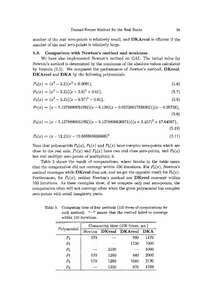
5.3. Comparison with Newton's method and weaknessWe have also implemented Newton's method on GAL. The initial value for

Newton's method is determined by the maximum of the absolute values calculatedby formula (2.5). We compared the performance of Newton's method, DKreal,DKAreal and DKA by the following polynomials.

P4(x) = (x2 -3.2)(x2 +0.0001),

P5 (x) _ (x2 — 3.2){(x — 3.5) 2 + 0.01},

P6(x) = (x2 — 3.2){(x — 9.57) 2 + 0.01},

P7(x) = (x — 5.1378890651692)(x — 5.138)(x — 0.057396173363021)(x — 0.05738),

(5.9)

P8 (x) = (x — 5.1378890651692)(x — 5.1378890630871){(x+ 3.457) 2 + 17.645671 ,

(5.10)

P9 (x) = (x — 12.2)(x — 19.666666666666) 3. (5.11)

Note that polynomials P4 (x), P5 (x) and P6 (x) have complex zero-points which areclose to the real axis, P7(x) and P8 (x) have two real close zero-points, and P9(x)

has real multiple zero-points of multiplicity 3.Table 5 shows the result of computations, where blanks in the table mean

that the computation did not converge within 100 iterations. For P4(x), Newton'smethod converges while DKreal does not, and we get the opposite result for P6 (x).Furthermore, for P5 (x), neither Newton's method nor DKreal converge within100 iterations. As these examples show, if we compute only real zero-points, thecomputation often will not converge often when the given polynomial has complexzero-points with small imaginary parts.

Table 5. Computing time of four methods (100 times of computations for

each method). "—" means that the method failed to converge

within 100 iterations.

(5.6)

(5.7)

(5.8)

PolynomialComputing time (100 times, ms.

Newton DKreal DKAreal DKA

P4 370 — 690 1170

P5 — — 1730 1000

P6 — 2100 — 1090

P7 670 1280 840 2000

P8 570 1290 1080 2130

P9 — 1330 870 1760


Tables 6 and 7 show accuracies of calculated zero-points of P7(x) and P8(x),

respectively, where inaccurate digits are underlined and we show only the real partsfor DKA. For each zero-point computed, its accuracy is not much different amongthe algorithms.

Table 6. Accuracies of computed real zero-points of P7(x).

Method Real zero-points

Newton 5.1378890651343 5.1380000000349 0.057396173362996 0.057380000000025

DKreal 5.1378890651439 5.1380000000376 0.057396173362978 0.057380000000071

DKAreal 5.1378890651439 5.1380000000376 0.057396173362978 0.057380000000071

DKA 5.1378890651302 5.1380000000311 0.057396173362958 0.057380000000088

Table 7. Accuracies of computed real zero-points of P8 (x).


Newton 5.137889 1215841 5.1378890066722

DKreal 5.137889 1318238 5.1378889991241

DKAreal 5.137889 1189296 5.1378890066883

DKA 5.1378890857556 5.1378890413680

For P9(x), Sturm's method fails to calculate correct number of the real zero-points, hence we gave correct number of the real zero-points to methods exceptfor DKA to calculate real zero-points. Table 8 shows accuracies of calculatedzero-points of P9(x). Newton's method fails to give all the real zero-points, whileDKreal, DKAreal and DKA succeed, by the following reason. In Newton'smethod, we perform deflation of polynomial after calculating each zero-point.Hence, if one of multiple zero-points is calculated with a low accuracy, then co-efficients in the deflated polynomial become inaccurate and Newton's method doesnot converge. On the other hand, the other methods calculate all the real zero-points including multiple zero-points, although accuracies of approximations for the

Table 8. Accuracies of computed real zero-points of P9(x).

Newton's method failed to calculate all the real zero-points.


Newton - - - 19.666985842244

DKreal 12.200000000000 19.666327629088 19.666713528554 19.666999258452

DKAreal 12.200000000000 19.666327629088 19.666713528554 19.666999258452

DKA 12.200000000000 19.666346248713 19.666732891919 19.666921927080


multiple zero-points become low.We see that, so long as correct number of the real zero-points is given, DKreal

and DKAreal give approximations for all the real zero-points even if there existmultiple zero-points.

6. Discussion

In this paper we have proposed two methods for calculating the real zero-points of a real univariate polynomial, on the basis of Durand-Kerner method.In the first method we calculate the real and the complex zero-points separatelyby a new setting of initial values for Durand-Kerner method, and in the secondmethod we calculate only the real zero-points of the polynomial. Furthermore, onthe basis of Smith's theorem, we have given a method to estimate the errors of theapproximations in the second method.

As we have seen in the experiments, algorithm DKreal has an advantage overNewton's method in that it calculates upper bounds of the errors of approximationssimultaneously. However, the experiments also show that, in the case that thereexist complex zero-points with very small imaginary parts, both Newton's method

and DKreal may not converge correctly. Therefore, in application, we had betteruse DKA if we have no information on the zero-points. In the case we alreadyknow good approximations of real zero-points and there does not exist complexzero-points with very small imaginary parts, we had better choose DKreal if thenumber of real zero-points is relatively small, or DKAreal if the number of real

zero-points is relatively large.In this paper, we have assumed that the number of real zero-points can be

calculated by Sturm's method. However, this assumption falls down in general ifthe given polynomial has multiple or close zero-points. How to calculate the numberof real zero-points correctly for polynomial with multiple or close zero-points is anopen problem, and we are now attacking this problem.

References

[ 1 ] O. Aberth, Iteration methods for finding all zeros of a polynomial simultaneously.Math. Comp., 27 (1973), 339-344.

[ 2 ] E. Durand, Solutions Numériques des Equations Algébriques (Tome I). Masson, Paris, 1960.[ 3 ] P.P. Fraigniaud, The Durand-Kerner polynomials roots-finding method in case of multiple

roots. BIT, 31, No.1 (1991), 112-123.[ 4 ] M. Iri, Numerical Analysis (in Japanese). Asakura Publishing Co., Tokyo, 1981.

[ 5 ] I.O. Kerner, Ein Gesamtschrittverfahren zur Berechnung der Nullstellen von Polynomen.

Numer. Math., 8 (1966), 290-294.[ 6 ] M. Natori, Numerical Analysis and its Applications (in Japanese). Corona Publishing Co.,

Tokyo, 1990.[7] L. Pasquini and D. Trigiante, A globally convergent method for simultaneously finding

polynomial roots. Math. Comp., 44, No.169 (1985), 135-149.[ 8 ] M.S. Petkovic, D.D. Herceg and S.M. Ilic, Point Estimation Theory and its Applications.

Institute of Mathematics, University of Novi Sad, Novi Sad, 1997.[9] T. Sasaki, Formula manipulation system GAL. Computing in High Energy Physics '91 (eds.

Y. Watase and F. Abe, Tsukuba, 1991), Universal Academy Press, Tokyo, 1991, 383-389.


[10] B.T. Smith, Error bounds for zeros of a polynomial based upon Gerschgorin's theorems.J. ACM, 17, No.4 (1970), 661-674.

[11] T. Takagi, Lectures in Algebra (in Japanese, revised ed.). Kyóritsu Publishing Co., Tokyo,1965.

[12] T. Yamamoto, S. Kanno and L. Atanassova, Validated computation of polynomial zeros bythe Durand-Kerner method. Topics in Validated Computations (Oldenburg, 1993), North-Holland, Amsterdam, 1994, 27-53.

Durand-Kerner method for the real roots

Documents