dukler-1980

subscripts

b = boiling point value C = critical value calc = calculated value exp = experimental value a J = components ij (r) = reference R = reduced value

LITERATURE CITED

Holm, L. W. and A. Josendal, “Mechanisms of Oil Displacement by

Holm, L. W., “Status of C 0 2 and Hydrocarbon Miscible Oil Recovery

Kesler, M. G. and B. I. Lee, “Improve prediction of enthalpy of frac-

Carbon Dioxide,” 1. Petroleum Technol., 26 (Dec. 1974).

Methods,”!. Petroleum Technol., 28 (Jan. 1976).

tions,” Hydrocarbon Process., 153 (March, 1976).

de Nevers, N. H., “A Calculation Method for Carbonated Water Flood- ing,” SOC. Pet. Eng. !., 9 (March, 1974).

Reid, R. C., J. M. Prausnitz and T. K. Shenvood, The Properties of Gases and Liquids, 3rd ed., McGraw-Hill, New York (1977).

Simon, R. and D. J. Graue, “Generalized Correlations for Predicting Solubility, Swelling and Viscosity Behavior of C02-Crude Oil Sys- tems,”f. Petroleum Technol., 102 (Jan. 1965).

Spencer, C. F. and S. B. Adler, “A Critical Review of Equations for Predicting Saturated Liquid Density,”!. Chem. Eng. Data, 23, 82 (1978).

Teja, A. S., “Binary Interaction Coefficients for Mixtures Containing the n-alkanes,” Chem. Eng. Sci., 33, 609 (1978).

Teja, A. S., “A Corresponding States Equation for Saturated Liquid Densities. I. Applications to LNG,” AZChE J . , 26, 000 (1980).

Watson, K. M., E. F. Nelson and G. B. Murphy, “Characterization of Petroleum Fractions,” Znd. Eng. Chem., 27, 1460 (1935).

Manuscript receioed June 7, 1979, and accepted October 1 1 , 1979

Modelling Flow Pattern Transitions for Steady Upward Gas-Liquid Flow in Vertical Tubes

YEHUDA TAITEL and

DVORA BORNEA School of Engineering

Tel Aviv University Ramat Aviv, lsmel

’ - and

A. E. DUKLER Models for predicting flow pattern transitions during steady gas-liquid flow in vertical tubes are developed, based on physical mechanisms suggested for each transition. These models incorporate the effect of fluid properties and pipe size Deportment of Chemical Engineering and thus are largely free of the limitations of empirically based transition maps or University of Houston correlations. Houston, Texas 77004

SCOPE When gas-liquid mixtures flow in a conduit, the two phases

may distribute in a variety of patterns. The particular pattern one observes depends on the flow rates, the fluid properties and the tube size. Figure 1 shows the expected patterns for a 5.0 cm diameter vertical pipe, flowing water and air at low pressure. Heat and mass transfer rates, momentum loss, rates of back mixing and residence time distributions all vary greatly with flow pattern. Given the existence of any one pattern, it is possible to model the flow so as to predict the important process design parameters. However, a central task is to predict which flow pattern will exist under any set of operating conditions as

well as the ffow rate pair at which transition between flow patterns will take place.

Many two-phase flow pattern maps have been proposed. Most of these have been based primarily on experiments and thus were limited to the conditions near those of the measurements. It is the objective of this work to suggest physically based mechanisms which underlie each transition and to model the transitions based on these mechanisms. The results are applicable for a wider range of properties and conduit sizes than would be expected from empirically determined transitions.

CONCLUSIONS AND SIGNIFICANCE

Models are developed to predict the transition boundaries between the four basic flow patterns for gas-liquid flow in vertical tubes: bubble, slug, churn and dispersed-annular. It is suggested that churn flow is the development region for the

slug pattern and that bubble flow can exist in small pipes only at high liquid rates, where turbulent dispersion forces are high. Each transition is shown to depend on the flow rate pair, fluid properties and pipe size, but the nature of the dependence is different for each transition, because differing mechanisms -

~ 1 - 1 5 4 1 - 8 0 - 3 ~ 2 ~ ~ n 3 4 5 - $ 0 1 25 0 TIre A n ~ e r r ~ a n Institute oi Chemical Engineers, The theoretical predictions are in god 1980 agreement with a variety of published flow maps based on data.

AlChE Journal (Vol. 26, No. 3) May, 1980 Page 345

t t I

Bubble SlUll flow flow

t

Churn flow

t

. . _ . . . . . . . , . _

. . . . , . . . . . . . . . . . . . . . . .. -id Annular

flow

Figure 1. Flow patterns in vertical flow.

Predicting flow patterns for upward flow of gas-liquid mixtures in vertical pipes is as yet an unresolved problem. A typical approach has been to coordinate experimental observation by plotting transition boundary lines on a two-dimensional plot. The coordinates have been more or less arbitrarily chosen, and the lack of physical basis for their selection has limited their generality and accuracy. Maps prepared from data taken for one pipe size and fluid properties are not necessarily valid for other sizes or properties. Further, there is poor agreement among most published maps.

Part of the problem arises from lack of agreement in the description and classification ofthe flow patterns and the subjec- tivity of the observer. The flow is often very chaotic and difficult to describe, which leaves room for personal judgment and interpretation. Hubbard and DukIer (1966) proposed a method for fingerprinting flow regimes using spectral analysis of wall pressure fluctuations, but this method has not generally been adopted .

In this work, the main flow patterns are first described. To correctly interpret and predict the conditions for transition, it is essential to understand the mechanism by which the transition from one flow pattern to another takes place. Physical models that describe transitions are presented and used to develop theoretically-based transition equations, which can be used to construct maps. The approach here is similar in principle to that presented by Taitel and Dnkler (1976) for horizontal flow systems. Since the maps presented are constructed on a physical basis, it is expected that they can be utilized over a wider range of flow conditions and fluid properties. Finally, the newly developed predictions are compared with those of recent maps which coordinate experimental data.

FLOW DESCRIPTION

When gas-liquid mixtures flow upward in a vertical tube, the two phases may distribute in a number of patterns, each characterizing the radial and/or axial distribution of liquid and gas. The flow is usually quite chaotic, and these phase distributions are dimcult to describe. We will follow the lead of Hewitt and Hall-Taylor (1970) who designate four basic patterns for upflow as follows:

1. Rubble Flow: The gas phase is approximatcly uniformly distributed in the form of discrete bubbles in a continuous liquid phase.

2. Slug Flow: Most of the gas is located in large bullet shaped bubbles which have a diameter almost equal to the pipe diameter. They move uniformly upward and are some-

times designated as “Taylor bubbles.” Taylor bubbles are separated by slugs of continuous liquid which bridge the pipe and contain small gas bubbles. Between the Taylor bubbles and the pipe wall, liquid flows downward in the form of a thin falling film. (This pattern has been designated by others as plug, or piston, flow at low rates where the gas liquid boundaries are well defined, and as slug flow at higher rates where the boundaries are less clear.)

3. Churn Flow: Churn flow is somewhat similar to slug flow. It is, however, much more chaotic, frothy and disordered. The bullet-shaped Taylor bubble becomes narrow, and its shape is distorted. The continuity of the liquid in the slug between successive Taylor bubbles is repeatedly de- stroyed by a high local gas concentration in the slug. As this happens, and liquid slug falls. This liquid accumulates, forms a bridge and is again lifted by the gas. Typical of churn flow is this oscillatory or alternating direction of motion of the liquid. (Some observers refer to a froth flow pattern for higher liquid and gas rates where the system appears more finely dispersed.)

4. Annular Flow: Annular flow is characterized by the continuity of the gas phase along the pipe in the core. The liquid phase moves upwards partly as wavy liquid film and partially in the form of drops entrained in the gas core. (Annular flow has been described as a whispy-annular pattern when the entrained phase is in the form of large lumps or “wisps.” Froth, mist or semi-annular flow patterns have also been used to describe the churn and annular patterns.)

EXISTING FLOW PATTERN MAPS

There is a wide variety of flow pattern maps for vertical flow in the literature. I t is important to understand that these maps propose transition boundaries in a two-dimensional coordinate system as determined from experiment, these experiments, in some cases, being those ofthe author, and in other cases coming from observations ofothers. The selection of coordinates for the published maps has been of two basic types:

a. One group uses dimensional coordinates such as superficial velocities U , and ULs (Sternling 1965, Wallis 1969) or superficial momentum flux, p&& and pJ& (Hewitt and Roberts 1969). Given any single pipe size and set of fluid properties, these coordinates will map the transitions, but there is no reason to expect that the location of these transition curves will be unchanged for changes in these variables. Govier and Aziz (1972) attempt to mod+ these dimensional coordinates for systems other than air- water by considering property ratios between the fluids of interest and that of the air-water system. However, there is no basis in theory to suggest this generalizes the results in any way.

b. A second group represents the results by dimensionless coordinates, in the hope that the result will apply to line sizes and fluid properties other than those of the data used to locate the curves. In the absence of a theoretical basis, the use of dimensionless coordinates is no more general than the use ofdimensional ones. Further, it will be shown below that one pair of dimensionless groups does not characterize the variety of transition boundaries that exist. The dimensionless groups selected by Duns and Ros (1963) and also used by Gould (1974) seem arbitrary. Griffith and Wallis (1961) were the: only investigators who attelnpted to invoke theory to arrive at suitable cwrdi- nates. They were able to show that the dimensionless coordinates U$gD and U<;.&.y controlled the transition from the slug to annular patterns. The theory was not completed sufficiently to provide an analytical expression for the transition curve, and experimental data were used to provide for the unknown constants. As discussed, the use of these same coordinates for the other transitions is open to question.

Page 346 May, 1980 AlChE Journal (Vol. 26, No. 3)

Comparisons between these various maps reveal differences both as to absolute value and trend. The problem seems to arise from the fact that in almost all cases, the transition boundaries are empirically located and do not rest in suitable physical models. Thus, it is important to place a theoretical basis under the transition relationships, both to improve the generality of the prediction and for classifying the experimentally observed flow patterns.

TRANSITION MECHANISMS

In order to predict the conditions under which transition between flow patterns will take place, it is essential to understand the physical mechanisms by which such transitions occur. In this way, the influence of fluid properties and pipe size-as well as flow rates-can be accounted for naturally in the equations which result. And, these can be expected to apply generally without the need for “scale-up” rules or procedures. The task of constructing flow transition boundary curves or maps from these equations is usually straightforward. But there is considerable disagreement among authors as to the mechanism for these transitions. In the following, each transition is analyzed, a physical mechanism proposed, and then the conditions for transition mathematically modelled.

The Bubble-Slug Transition

Transition from the condition of dispersed bubbles observed at low gas rates to slug flow requires aprocess of agglomeration or coalescence. Only in this way can the discrete bubbles combine into the larger vapor spaces, having a diameter nearly that of the tube, with lengths of 1-2 diameters which are observed at the transition to slug flow. As the gas rate is increased, the bubble density increases. This closer bubble spacing results in an increase in the coalescence rate. However, as the liquid rate increases, the turbulent fluctuations associated with the flow can cause breakup of larger bubbles formed as a result ofagglomera- tion. If this breakup is sufficiently intense to prevent recoales- cence, then the dispersed bubble pattern can be maintained. Thus, to predict conditions for this transition, we must deter- mine when each of these factors will dominate the process.

When gas is introduced at low flow rates into a large diameter vertical column of liquid (flowing at low velocity), the gas phase is distributed into discrete bubbles. Many studies of bubble motion demonstrated that if the bubbles are very small, they behave as rigid spheres rising vertically in rectilinear motion. However, above a critical size (about 0.15 cm for air-water at low pressure) the bubbles begin to deform, and the upward motion is a zig-zag path with considerable randomness. The bubbles randomly collide and coalesce, forming a number of somewhat larger individual bubbles with a spherical cap similar to the Taylor bubbles of slug flow, but with diameters smaller than the pipe. Thus, even at low gas and liquid flow rates, bubble flow is characterized by an array of smaller bubbles moving in zig-zag motion and the occasional appearance of larger, Taylor-type bubbles. The Taylor bubbles are not large enough to occupy the cross section of the pipe so as to cause slug flow in the manner described above. Instead, they behave as free rising spherically capped voids, in the manner originally described by Taylor. With increases in gas flow rate, at these low liquid rates, the bubble density increases and a point is reached where the dispersed bubbles become so closely packed that many colli- sions occur and the rate of agglomeration to larger bubbles increases sharply. This results in a transition to slug flow.

Experiments suggest that the bubble void fraction at which this happens is around 0.25 to 0.30 (Griffith and Synder 1964). A semi-theoretical approach to this problem was given by Radovicich and Moissis (1962), by considering a cubic lattice in which the individual bubble fluctuates. They postulated that the maximum void fraction is reached when the frequency of collision is very high, and it was shown that this happens around void fraction of 0.30.

10

1.0 A

u 0) u) \ E Y

3 0.1 3

0.01

I I I . FINELY DISPERSED

BUBBLE (II) C

JNULAR

BUBBLE (II)

0. I I .o 10.0 100 U,, (rnlsec)

Figure 2. Flow pottern map for vertical tubes 5.0 cm dia., air-water at 25”C, 10 N/sq.cm.

An alternative approach is to consider this problem from the point of view of maximum allowable packing of the bubbles. If we consider the bubbles to have spherical shape and arranged in a cubic lattice, the void fraction of the gas can be, at most, 0.52. However, as a result of their deformation and random path, the rate of collision and coalescence will increase sharply at void fractions well below this lattice spacing at which they touch. Therefore, the closest distance between the bubbles before transition must be the one which permits some freedom of motion for each individual bubble. If the spacing between the bubbles at which coalescence begins to increase sharply is assumed to be approximately half their radius, this corresponds to about 25% voids. While this approach is not a prediction of the void fraction at transition from first principles, it does provide a reasonable interpretation of the experimental data. Published data agree in that the void fraction in bubbly flow rarely exceeds 0.35, whereas for void fractions less than 0.20 coalescence is rarely observed (Griffith and Wallis 1961). Thus, at liquid rates low enough so that bubble breakup due to turbulence is small, the criteria for transition from bubbly to slug flow is that the void fraction reaches 0.25.

If the gas bubbles rise at a velocity UG, this velocity is related to the superficial gas velocity U G S by

where a is the void fraction. Likewise, the average liquid velocity is given in terms of the liquid superficial velocity as

U L S U L = -

1 - a

Designating Uo as the rise velocity of the gas bubbles relative to the average liquid velocity, equations (1) and (2) yield

1 - a - (1 - a)Uo U L S = u,, - a (3)

The rise velocity Uo of relatively large bubbles has been shown by Harmathy (1960) to be quite insensitive to the bubble size and given by the relation

(4)

Substituting Equation (4) into (3), and considering the transition to slug flow to occur when a = aT = 0.25 results in an


equation characterizing this transition for conditions where the dispersion forces are not dominant.

Once fluid properties are designated, the theoretical transition curve can be plotted on U L s vs U G S coordinates and will remain invariant with tube size. Such a curve is shown in Figure 2 for the water-air system of25'C and 10 N/cm2 where it is designated as curve A. At higher gas and liquid flow rates, where the bubble rise velocity relative to the liquid velocity is negligible, the theoretical transition curve is linear, with a slope of unity in these log coordinates. On the other hand, at low liquid rates where liquid velocity is negligible, the boundary of the bubble region is controlled by the free rise velocity of the bubbles and is essentially independent of liquid rate.

This method for predicting the bubble-slug transition is similar in principle to that of Griffith and Wallis (1961). They used a = 0.18 as a criteria for maximum packing and set Uo equal to a constant of 0.24 m/sec which is the rise velocity predicted from Equation (4) for an air-water system. The results were, therefore, not general for fluids other than air-water.

At higher liquid flow rates, turbulent forces act to break and disperse the gas phase into small bubbles even for vapor void fractions higher than 0.25. The theory ofbreakup of immiscible fluid phases by turbulent forces was given by Hinze (1955) and recently confirmed by Sevik and Park (1973). Hinze determined that the characteristic size of the dispersion results from a balance between surface tension forces and those due to turbulent fluctuations. His study led to the following relationship for the maximum stable diameter of the dispersed phase, d,,,.

where E is the rate of energy dissipation per unit mass. Hinze's investigation explored dispersion under non-coalescing conditions which can be realized only at very low concentrations of the dispersed phase. He applied his formula to the data of Clay (1940) for droplet breakup at low concentration of dispersed phase and found k to be equal to 0.725. Sevik and Park (1973) developed theoretical values of k by considering the natural frequency of a bubble or drop in its lowest order mode of vibration. Assumipg this natural frequency to be the ratio of the rms velocity fluctuation in the turbulent stream to the diameter of the drop or bubble, they were able to prove that k = 0.68 for drops (density of dispersed phase >> density of continuous phase) and k = 1.14 for bubbles (density of dispersed phase << density of the continuous phase). Experimental measurements ofbubble breakup in a liquid jet showed remarkable experimental agreement with k = 1.14.

The rate of energy dissipation per unit mass for turbulent pipe flow, e, is

where

(7)

Substitution of Equation (8) into (7) shows that turbulent breakup of bubbles exists for all liquid rates high enough to cause turbulent flow. However, if the bubble size produced by the breakup process is large enough to permit deformation, then at values of a approaching 0.25, the large Taylor bubbles characteristic of slug flow again are formed by the process of coalescence. Thus, the turbulent breakup process can prevent agglomeration only if the bubble size produced is small enough to cause the bubbles to remain spherical. The bubble size at which this occurs is given by Brodkey (1967) as

(9)

Ford,, > dct.rt the bubbie rise velocity is almost independent of bubble size and is given by Equation (4), but decreases very rapidly for bubble diameters below dedt. Once turbulent fluctuations are vigorous enough to cause the bubbles to break into this small critical size, coalescence is suppressed and the dispersed bubble flow pattern must exist even for a > 0.25. From Equations (6), (7) and (9), the conditions for this transition can be found. Note that in this region of high flow rate the slip velocity can be neglected and the gas holdup calculated simply by

The friction factor needed in Equation (8) can be predicted by the Blasius equation based on the superficial mixture velocity and the liquid kinematic viscosity, namely

U M D -' f = c(-) V L

where C and n are taken as 0.046 and 0.2, respectively. Combin- ing Equation (7) to (11) results in a dimensionless expression relating the flow rates, properties and pipe size at which turbulent induced dispersion takes place.

Once the fluid properties and pipe size are set, Equation (12) defines the relationship between the values of UGs and U L S

above which slug flow cannot exist. For air-water at 25°C and 10 N/cm2 pressure this result is shown in Figure 2 for a 5.0 cm diameter pipe and is designated by curve B. However, regard- less of how much turbulent energy is available to disperse the mixture, bubble flow cannot exist at packing densities above a = 0.52. Thus, the B curve delimiting dispersed bubble flow must terminate at the curve C which relates U,, and UGs for a = 0.52.

This approach neglects the effect of increasing holdup on the process ofcoalescence and on the resulting bubble size. Calder- bank (1958) investigated the balance between bubble breakup and coalescence in determining bubble size in mechanically stirred gas-liquid columns. There he showed that the bubble size varied with the holdup to the one halfpower. However, the mechanism for such coalescence, namely, agitator causing eddy-like motion of the bubbles, is not present here. With flow induced radial motions, the effect of holdup is likely to be less significant; however, its quantitative influence cannot be evaluated at this time.

Thus, the bubbly flow pattern can be seen to exist in zones I and I1 of Figure 2. In zone I to the left of curve A and below B, one predicts the presence of deformable bubbles which move upward with a zig-zag motion with Taylor-type bubbles occa- sionally appearing in the liquid. In zone I1 above curve B and to the left of C, one observes a more finely dispersed bubble system without any Taylor bubbles. To the right ofA and below B in zone 111, one expects to see the slug pattern.

Still a different transition mechanism comes into play in the special case of tubes of small diameter. Consider zone I of Figure 2 where one observes discrete deformable bubbles rising in zig-zag paths and the occasional appearance of a Taylor bubble. The velocity of rise of the deformable bubbles relative to the liquid, Uo, is given by Equation (4) and depends only on the properties of the fluids. The rise velocity of the Taylor bubbles relative to the mean velocity of the liquid on the other hand is given by (Nicklin et al. 1962).

UG = 0 . 3 5 d Z (13) and is property independent. Whenever Uo > U G the rishg bubbles approach the back of the Taylor bubble coalescing with it, increasing its size. Under these conditions bubbly flow cannot exist in zone I. On the other hand, when Uo < UG the Taylor bubble rises through the array of distributed bubbles and the relative motion of the liquid at the nose of the Taylor bubble


10

I .a u Q) u) \ E y 0.1

3 v) -I

0.01

I I I FINELY DISPERSED /

I I001 500

I I II I I I

l ~ / D = r S o 1200 I

ANNULAR ( P I

I 0. I 1.0 10 100

UGs( m/sec)

Figure 3. Flow pattern map for vertical tubes 2.5 cm dio., air-water at 25”C, 10 N/cm2.

sweeps the small bubbles around the larger one, and coalescence does not take place. The properties of air-water at low pressure are such that U o = U G at D -- 5.0 cm. Thus, for tubes smaller than 5 cm in diameter, no bubbly flow can exist below the curve B and the entire zone I and 111 exist as the slug flow pattern. Only at high liquid rates, zone 11, can bubbly flow exist for small tubes where dispersion occurs due to turbulence. The flow pattern map for 2.5 cm diameter tubes with the system air-water is shown in Figure 3, where zones I and 111 are combined. A system having a small diameter is one which satisfies the criterion below.

(14)

It is of interest that the range of diameters used in most laboratory air-water experiments, i.e., 2-6 cm, spans this critical diameter of 5.0 cm. This accounts for the apparent differences in observations which have been reported. It also shows that for this particular transition, experimental data taken on small pipes cannot be scaled to larger diameters. It is only through an understanding of mechanisms, as discussed here, that rational size scaling can be accomplished.

Slug-Churn Transition

The slug flow pattern develops from a bubbly pattern when the gas flow rate increases to such an extent that it forces the bubbles to become closely packed and coalesce. At this point, “Taylor” type bubbles are formed which, if the process ofcoalescence continues, occupy most of the pipe cross sectional area and are axially separated by a liquid slug in which small bubbles are dispersed. The liquid confined between the bubble and the pipe wall flows around the bubble as a falling film.

As the gas flow rate is increased still more, a transition to churn flow occurs. There is considerable difficulty in accurately identifying the slug-churn transition because there is confusion as to the description ofthe churn flow itself. Some identify churn flow on the basis of the froth that appears within the gas region, and these investigators describe the pattern as frothy. Others associate churn flow with the instability of the liquid film adjacent to the Taylor bubble. We characterize the churn flow pattern as that condition where oscillatory motion of the liquid in observed. In slug flow, the liquid between two Taylor bubbles moves at a constant velocity and its front as well as its tail have

constant speed. In churn flow, the liquid slug is too short to support a stable liquid bridge between two consecutive Taylor bubbles. The falling film around the bubble penetrates deeply into the liquid slug creating a highly agitated aerated mixture at which point the liquid slug is seen to disintegrate and to fall in a rather chaotic fashion. The liquid re-accumulates at a lower level at the next slug where liquid continuity is restored and the slug then resumes its upward motion. Thus, one observes an oscillatory motion of the liquid, which we consider the characteristic identification of churn flow.

There have been several mechanisms proposed for transition to the churn pattern. Nicklin and Davidson (1962) suggested that the transition to churn flow occurs when the gas velocity relative to the falling liquid film around the Taylor bubble approaches the condition of flooding.

Moissis (1963) attributed this transition to Helmholtz instability of the liquid film bounding the Taylor bubble. The Helm- holtz instability criterion was applied for an infinitely thick gas region and very thin liquid film using Feldman’s (1957) result that the wave length is 10 times the film thickness. The analysis is inconsistent since Feldman’s theory is not based on Helm- holtz type analysis. Furthermore, Feldman’s calculation for the stability criterion is in error.

Griffith and Wallis (1961) suggested that transition from slug to annular flow occurs when the individual Taylor bubbles becomes very (infinitely) long. Their predicted transition to annular flow occurs at much lower gas rates than indicated by experiment which suggests that this mechanism might account for the slugkhurn transition instead. No predictive model was presented, and their transition curve was finally obtained solely from experimental data.

Careful and repeated observations of the slug-churn flow patterns on 2.5 and 5.0 cm diameter test sections in our labora- tories suggest a rather different mechanism than any of the above. These observations indicate that the churn flow pattern is an entry region phenomenon associated with the existence of slug flow further along the pipe. That is, whenever one observes slug flow, the condition near the entry appears to be churning. Furthermore, the entry length, or the distance that such churning can be observed before stable slug flow takes place, depends on the flow rates and pipe size.

The process of developing a stable slug near the entrance section can be described as follows: At the inlet the gas and liquid which are introduced form short liquid slugs and Taylor bubbles. A short liquid slug is known to be unstable, and it falls back and merges with the liquid slug coming from below causing it to approximately double its length. In this process, the Taylor bubble following the liquid slug overtakes the leading Taylor bubble and coalesces with it as the slug between the two bubbles collapses. This process repeats itself, and the length ofthe liquid slugs as well as the length of the Taylor bubbles increase as they move upwards, until the liquid slug is long enough to be stable and form a competent bridge between two consecutive Taylor bubbles. Between the inlet and the position at which at stable slug is formed, the liquid slug alternately rises and falls, and this is precisely the condition of churn flow. As the gas rate increases, it is evident that the length of this entrance region increases to the extent that it can occupy the entire length ofany test section. Thus, one should think ofchurn flow as an entrance phenomena. Since; in practice, all pipes are of a finite length, it would be useful to provide some estimates of the lengths over which churn flow is the predominant mode. With this objective, we develop a method for calculating the entry length required to develdp stable slug flow. The distance from the entrance to that length will be observed to be in the churn flow psitern.

Figure 4 shows a model of slug flow. Consecutive Taylor bubbles rise in a vertical pipe, separated by regions of liquid containing small bubbles. The Taylor bubbles rise at a velocity designated by UG. The liquid between the Taylor bubbles moves upwards at an average velocity U L . The bubble cavity is at nearly constant pressure, and the liquid film adjacent to the bubble flows downward as a free-falling film at a velocity, U f . Since the


"TAYLOR"

LIQUID

FALLING

BUBBLE\

A

0 0 0 0 0 0 0 0 0 0 0 0 0 0 0 0 0 0 0 0

\

eG I I

B

0 0 0 0 0 0 0 0 0 0 0 0 0 0 0 0 0 0 0 0

Figure 4. Slug flow geometry.

slug flow pattern is developed when (YT = 0.25, the liquid slug between the Taylor bubbles is assumed to contain small bubbles at this bubble density. Further, the dispersed bubbles are assumed to be confined to the region between the Taylor bubbles, thus moving with the Taylor bubble velocity U G . Although observations of slug flow show that some small bubbles are swept into the liquid film around the Taylor bubble, this as- sumption has little effect on the result.

The velocity of the Taylor bubble is given quite accurately by the relation (Nicklin e t al. 1962),

UG = 1.2 UL + 0 . 3 5 v s (15) In this equation the second term on the R.H. S. describes the rise velocity of a large bubble in stagnant liquid. It was derived theoretically by Davies and Taylor (1949) and by Dumitrescu (1943). The first term of the R. H. S. adds the liquid velocity at the centerline, since 1.2 is approximately the ratio ofcenterline to average velocity in fully developed turbulent flow. The total volumetric flow rate, Q, is constant across any cross section. Therefore,

The Taylor gas bubble velocity can be solved directly by eliminating UL between (15) and (16) arriving at

1.2 ~ uM + 0 . 3 5 d S

1 + 1.2 ~

(17) 1 - a T u, =

CUT

1 - (YT

Using (16) the liquid velocity equals

Consider two consecutive Taylor bubbles (as shown in Figure 4). The first (top) bubble moves at a velocity given by Equation (15). The second (lower) bubble will move at the same speed when the slug length 1s is long enough so that the velocity profile

in the liquid at the front of the second bubble will be the same as that at the front of the first bubble, namely, the average velocity is UL and the centerline velocity is 1.2 U L . This is the situation to be expected when the slugs are long enough so that the turbulent velocity distribution in the liquid can b e fully reestablished before the next Taylor bubble appears. Then the velocity of the two consecutive Taylor bubbles is the same, the length of the liquid slug will remain constant with time and position in the direction of flow and stable slug flow exists.

But since the liquid slugs are shorter in the developing region, t h e velocity distribution in the liquid can be severely distorted by the flow reversal near the wall as a result of the falling film. Consider the velocity distributions in the planes A-A and B-B behind the leading Taylor bubble shown in Figure 4. If the liquid slug is long, far enough behind the trailing edge of the bubble (plane B-B), the velocity becomes that typical of turbulent flow. However, at A-A the flow is downward near the wallas a result of the falling film around the bubble. In order to main- tain mass continuity, the velocity at the centerline must increase. Since the velocity of a Taylor bubble depends on the centerline velocity plus its rise velocity, it is clear that for liquid slugs too short to reestablish the turbulent velocity distribution, the second bubble will overtake the first (Moissis and Griffith 1962). As a result, the two bubbles will coalesce, the liquid bridge between them will disintegrate, and fall to a lower level creating churn flow.

Experimental observations for water-air systems suggest that the length of a stable slug relative to this diameter, 1slD is fairly constant and independent of gas and liquid flow rates (Govier and Aziz 1972, Akagawa and Sakaguchi 1966). The minimum value of ls1D reported was 8. Studies in our laboratory, using very long, 2.5 and 5.0 cm diameter tubes, showed stable slug lengths approach 16D. The earlier observations can be considered the result of two slugs, each not quite of stable length, IslD = 8, which approach each other so slowly that they would never coalesce except in a long tube. By use of the very approximate argument which follows, it is possible to show that this stable length, lslD = 16, observed for ainvater, should be essentially independent of fluid properties or pipe diameter.

The liquid film falling along the Taylor bubble has an average velocity Uf and velocity relative to the liquid at plane A-A behind the bubble of (Uf + U,). Consider this liquid sheet as a two dimensional je t which enters a stagnant pool of liquid (the slug) at a uniform velocity, (Uf + U G ) . The axial velocity, U , in the liquid induced by the jet will depend on the distance x in the direction of the jet and y, the normal distance from the jet centerline. Both experimental and theoretical studies have shown that the ratio of U(x,y) to U,,,(o,y) varies as

where y is a universal constant approximately equal to 7.67 (Schlichting 1968). A stable slug is one which is long enough that the jet has been absorbed by the fluid and the velocities have slowed to that of the surroundings. In this case, we explore the distance x = ls which at the centerline, y = D/2, the velocity is essentially flat, say U/UmaX 5 0.05, and thus the normal turbulent distribution in the liquid slug is undistorted. Equation (19) shows that this takes place atlslD 2 16. This is, ofcourse, only an approximate argument because the falling film is a wall jet, not a free jet and the fluid is confined, not ofinfinite extent. However, Pate1 (1971) showed that the velocity distributions in a wall jet on the side of the velocity maximum away from the wall can be estimated as in a free jet. Since the falling film is so thin, the approximations used above become quite reasonable.

Entry Length for Churn Flow: Designate l E as the entry length of pipe required to establish stable slug flow and therefore the region that one would observe churning. Consider a coordinate x pointing downward from the trailing edge of the leading Taylor bubble as in Figure 4. The velocity at the center of the pipe, U,, varies from U G atx = 0 to 1.2 UL atx = 1s. Assume exponential variation with x as follows


The constant j3 determines the decay rate and was chosen at p = In 100 = 4.6 so that at x = 1s the decay will be 1%. The final results are not sensitive to the particular choice of j3, or to the particular profile assumed as long as U,(x = 0) = UG and Uc(x = Is) = 1.2 U L . Designating the leading bubble as the first and the trailing bubble as the second and using Equation (15) for calculating the velocities of the two consecutive bubbles, we obtain an approach velocity between two bubbles, -11, as

-? = U,, - Ucl = (Uc - 1.2 UL)e-oZ/‘S

= 0 . 3 5 d s e-Bx/‘s (21)

It is interesting to compare this result with that given by Moissis and Griffith (1962) who measured the velocity of aTaylor bubble that follows a leading bubble and correlated it empirically by the relationship

Using (21) and (17) our results for (YT = 0 (as in Moissis and Griffith’s case) can be expressed in the form

- e - . 2 8 7 5 ~ / D (23) % = I + 0.35 UCI 1.2 UMldgD + 0.35

While the form and constants in the second termof equation (23) seem quite different from Moissis and Griffiths Equation (B), the agreement in UcZ/Ucl is excellent for r /D > 3. For x/D less than three, our prediction is poor, probably because for this condition the two bubbles are very close and are near collapse. However, for the purpose of calculating the entry length, know- ing the approach velocity for bubbles separated by distances of the order of D is not important as will be seen below. The fact that this model derived without data agrees so well with the Moissis and Griffith data gives confidence for its use for other pipe sizes and fluid properties.

In calculating the entry length or length for churn flow, it is assumed that near the gas liquid inlet coalescence is instantane- ous and short Taylor bubbles as well as short liquid slugs are formed. The merging of the Taylor bubbles to larger gas bubbles and larger liquid slugs takes place when the second bubble overtakes the leading bubble. When they combine the volume, as well as the length, of the newly created Taylor bubble is doubled. Likewise, the liquid slug behind the leading bubble falls and merges with the liquid slug behind the second bubble to create a slug twice as long. At approximately the same time, the third and fourth bubbles will combine and again create a new bubble and new liquid slug of double length. This process will go on, and pairs of bubbles will coalesce as they move upward, doubling their length each time until a stable liquid slug of 1engthIslD = 16 is formed. The term 1s designates the length ofa stable slug while I , is the length of a slug formed during the period of coalescence. Because the last merger of two slugs of length lL = 8D is quite slow, we consider the entrance or churning length to exist up to the point where 1~ = 8D (or ZL = ls/2), the region of churn flow.

Integrating (21) gives the time needed for each merger as a function the distance, ZL,, between two consecutive bubbles

t , = ls [eolL1/fs - 11 (24) 0 . 3 5 j 3 q z

where i takes successive values of 0, 1, 2 ,3 . . . . Lettinglu take the sequence from 0 to 1~14, namely, k, = 1~14, 1~18, 1~116 . . . 0 yields an infinite series for t i whose sum multiplied by UG yields the estimated entrance length 1,.

or considering @ = 4.6 and I s = 16D yields

Substituting (17) into (26) for cuT = 0.25 yields

D

where Uu = UGS + ULs. This shows that thr dimensionless entry l ensh for churning depends on one parameter, namely, UMl V g D . The solution to this equation for a low pressure air-water system at several values of ZE/D is shown in Figures 2 and 3 for 5.0 and 2.5 cm diameter tubes where these curves are designated as “D.”

Figure 2 shows typical trends for pipe diameters larger than that needed to satisfy Equation (14), that is, pipe sizes where a bubbly flow pattern can be expected to exist. Note that the “D curves” delineating the transition between slug and churn flow terminate on the “A curve.” This A transition boundary represents the locus of points in the U L S - U G S plane where LY = 0.25 and for a < 0.25 only bubble flow can exist.

On the other hand, for the smaller pipe sizes represented in Figure 3 only slug flow is observed, even for a < 0.25. However, churning can be expected only when a > 0.25. Thus, the locus of Urn - U G S values for a = 0.25 is shown dotted on Figure 3 and still represepts the terminus of the D curves.

It is now possible to predict if churn flow will be observed at any axial position along the pipe. Assume that the point of observation is 200 diameters above the entry. Over the flow rate region to the left of the 1EID = 200 curve of Figure 2 and to the right ofthe A curve, slug flow will be observed. At flow rate pairs to the right of curve D, churn flow will be seen, providing the rate is not high enough to cause the annular pattern. Although churning is visualized as an entry region phenomenon, conditions where churn flow would be observed over the entire length of a tube can be shown to exist. For example, consider a 5.0 cm diameter pipe whose length is somewhat less than 2000. Values of ULs and Ucs located just to the right of the 1ElD = 200 curve of Figure 2 would result in churn flow being observed at all positions along the pipe. In other words, the entire tube consists of entry length for purposes of developing slug flow.

Tmnsition to Annular Flow

For high gas flow rates the flow becomes annular. The liquid film flows upwards adjacent to the wall, and gas flows in the center carrying entrained liquid droplets. The upward flow of the liquid film against gravity results from the forces exerted by the fast moving gas core. This film has a wavy interface and the waves tend to shatter and enter the gas core as entrained droplets. Thus, the liquid moves upwards, due to both interfacial shear and form “drag” on the waves and drag on the droplets. Based on the idea by Turner et al. (1968) applied to gas lift operations, we suggest that annular flow cannot exist, unless the gas velocity in the gas core is sufficient to lift the entrained droplets. When the gas rate is insufficient, the droplets fall back, accumulate, form a bridge and churn or slug flow takes place.

The minimum gas velocity required to suspend a drop is determined from the balance between the gravity and drag forces acting on the drop

or

(29)

The drop size is determined by the balance between the impact force of the gas that tends to shatter the drop and surface tension forces that hold the drop together. Hinze (1955) showed that the maximum stable drop size will be


I I I - O = 5.1 cm - (II) --6- 10 -

I 'b 1 il I I I I

0. I 1.0 10 100

UGs ( m /sec 1 Figure 5. Flow pattern map for vertical tubes crude oil-natural gas at

38"C, 670 N/sq.cm.

where K is the critical Weber number and takes a value between 20 and 30 for drops which are gradually accelerated.

Using (29) and (30) yields

(31) 1'4 [ d P L - Pc)1"4

U G = (g-) PG"*

As suggested by Turner e t al. (1969) values of I< = 30 and c d = 0.44 were selected. Note that K and c d appear in the power of %. Thus, the result for U G is quite insensitive to their exact values.

The gas velocity given by Equation (31) will predict the minimum value below which stable annular flow will not exist. While this analysis is applied to the droplets within the gas core, the same treatment can be usedfor the crests ofthe waves on the rising film, which are pictured as being supported by the gas stream in a manner similar to the support of the liquid droplets.

10

I .o

0. I

0.01

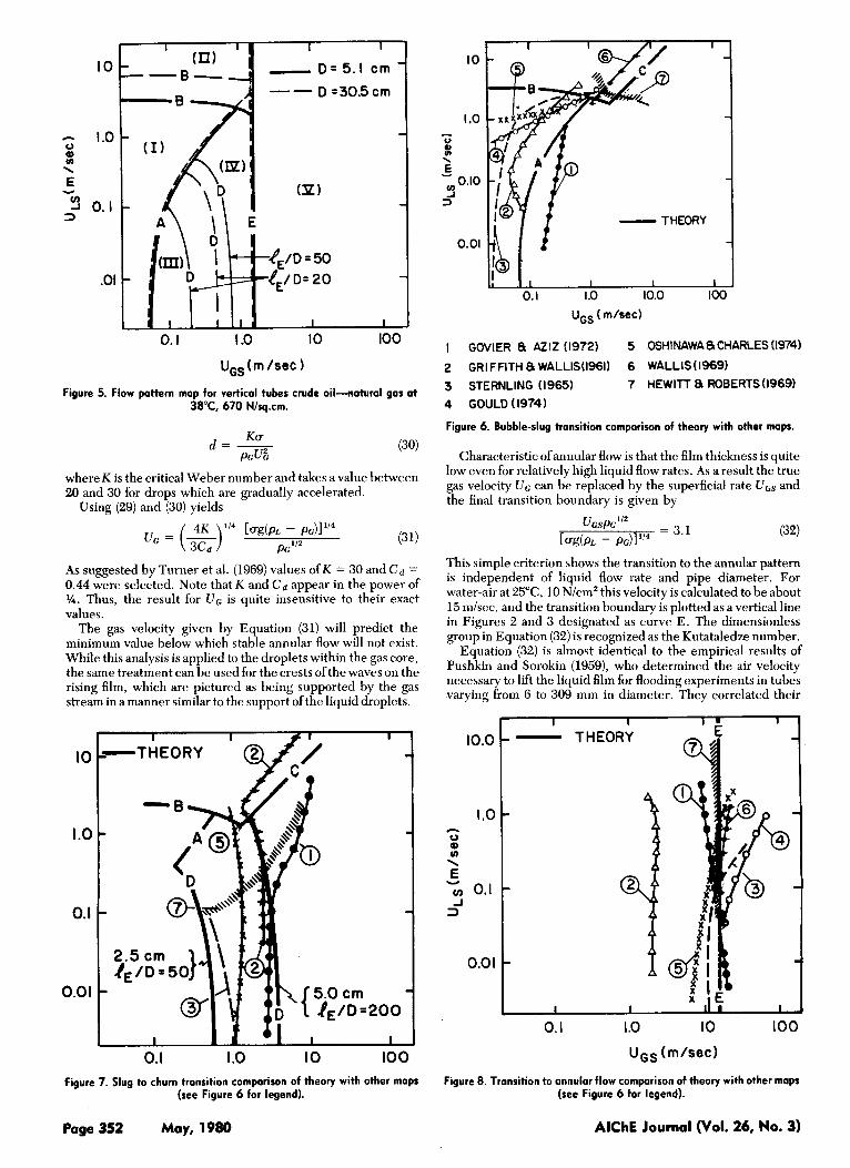
0. I I .o 10 100 Figure 7. Slug to churn transition comparison of theory with other maps

(see Figure 6 for legend).

I I I

-THEORY

10

1.0 - u \ %

3 E - 0.10

3

0.01

UGs ( m/sec)

I GOVIER 8 AZlZ (1972) 5 ~SHINAWA8CHARLES11974)

2 GRIFFITH 8 WALLIS(1961) 6 WALLIS(1969) 3 STERNLING (1965) 7 HEWITT Et ROBERTS(1969)

4 GOULD ( 1974)

Figure 6. Bubble-slug transition comparison of theory with other maps.

Characteristic ofannular flow is that the film thickness is quite low even for relatively high liquid flow rates. As a result the true gas velocity UG can be replaced by the superficial rate UGs and the final transition boundary is given by

This simple criterion shows the transition to the annular pattern is independent of liquid flow rate and pipe diameter. For water-air at 25"C, 10 N/cm2 this velocity is calculated tobe about 15 m/sec, and the transition boundary is plotted as a vertical line in Figures 2 and 3 designated as curve E. The dimensionless group in Equation (32) is recognized as the Kutataledze number.

Equation (32) is almost identical to the empirical results of Pushkin and Sorokin (1959), who determined the air velocity necessary to lift the liquid film for flooding experiments in tubes varying from 6 to 309 mm in diameter. They correlated their

I I I I . I c

10.0

I .o h 0 Q) u) \ E v v) 0.1 J 3

0.0 I

0. I I .o 10 100

U G S (m/sec)

Figure 8. Transition to annular flow comparison of theory with other maps (see Figure 6 for legend).


experimental results in terms of the Kutataledze number, except the constant 3.1 is replaced by the constant 3.2. While Pushkin and Sorokin arrived at their result by dimensional analysis and experiment, the above development places a theoretical basis under the result.

Fluid properties and pipe diameter enter into the transition equations to differing degrees depending on the transition being considered. To illustrate this effect, the location of the transition boundaries are shown in Figure 5, for a crude oil-natural gas system flowing at 30°C and 670 N/sq.cm pressure in pipes with diameters of 5.0 and 30.0 cm. Oil density was set at 0.65 g/cu.cm with natural gas at 0.05 gr/cu.cm with oil and gas viscosities of 0.5 and 0.015 cp.

It is useful to observe that the flow pattern transition boundaries can be readily obtained by hand calculation from the algebraic equations presented here for any pipe size and fluid properties.

Criterion for existence of bubble flow: Bubble to slug: E . 5 Bubble to dispersejbubble: Eq. 12 Slug to churn: Eq. 27 Annular: Eq. 32

Eq. 14

0 0 0 0

0 0 0 0 0 0

DISCUSSION AND CONCLUSIONS

In Figures 6 through 8, each of the transitions predicted by this theory are compared with published transition boundaries. As discussed above, these published transition boundaries are based on experimental data with little theoretical foundation. The wide discrepancy in the location of these curves emphasizes the role of observation and careful definition in the study of flow patterns. Location of curves in the published maps have been based on experiments in pipes, ranging in size from 2.0-6.0 cm in diameter, and with air-water at low pressure.

Transition A and B (Figure 6). The theory presented here identifies two bubble-slug transitions. Large Taylor type bubbles cannot exist above theoretical transition curve B due to turbulent dispersion. Transition to Taylor type bubbles or to churn flow takes place to the right of theoretical transition curve A. In the region between these two curves dispersed bubbles should appear for 5.0 cm and larger diameter pipes and Taylor bubbles should appear for 2.5 cm diameter pipes. "Bubble flow" has been used to describe the existence of both dispersed bubbles as well as Taylor bubbles that do not quite fill the pipe's cross section area. Note that, except for the Govier and Aziz curve, these two theoretical curves bound the range of the data. It thus includes all possible descriptions. If one designates the slug flow pattern only for these cases where Taylor bubbles which nearly fill the pipe exist and rise with a velocity given by Equation (15), then some of this ambiguity can be eliminated. Figures 9 and 10 show experimental data taken in our labora- tories in 2.5 and 5.0 cm tubes, which clearly demonstrate that for 2.5 cm tubes the A transition does not exist while for 5.0 cm tubes bubbly flow can be observed.

Transition D (Figure 7 ) . Since churn flow is an entry region phenomenon, the location of the slug-churn transition boundary depends on the point of observation along the pipe as discussed above. Theoretically predicted transition curves are shown for ZE

= 50D in a 2.5 cm pipe and 1, = 2000 in a 5.0 cm pipe. Considering the fact that there is no information on the location of the observation point for the published transitions, the results must be considered in remarkably good agreement with all published curves except that of Hewitt and Roberts (1969). The new experimental data in Figures 9 and 10 show excellent agreement with the theory at the lower liquid rates. At higher velocities, it is extremely difficult to visually discriminate between churn and slug flow.

Transition E (Figure 8). The vertical line representing transition E is compared with several published transitions in Figure 8. Except for the Grimth-Wallis curve, the theory is an excellent compromise between the various empirical curves proposed. At high liquid rates, there is increasing discrepancy both in trend

I (

h

0 Q) u) \ E Y

cn 9 0.

0.0

I I 1 I .THEORY -

BUBBLE A ..- I

o l o o ~ o o , + , I 0. I I 10 100

U ~ S ( m / s e c )

Figure 9. Comparison with new data water-oir, 25°C. 10 N/cm2, D = 2.5 cm, t = 13OD solid lines represent theory.

and magnitude between the theory and data curves as well as between the various sets of data. In this region of high liquid rate, the flow is extremely chaotic, and visual observations are not very specific. Figures 9 and 10 show that the theoretical prediction of this transition is in excellent agreement with our data taken in 2.5 and 5.0 cm diameter tubes.

Theoretically predicted transitions for upflow have been compared with the recommendations of many earlier investigators whose results have been based primarily on experimental measurements. There is considerable disagreement between the results of these various investigators. However, the theory presented here is in satisfactory agreement with the weight of the earlier experimental results. In addition, comparisons with new data taken in 2.5 and 5.0 cm tubes show good agreement, since the theory was developed without the use of experimental data.

I .o - 0 0) v) \ E Y

0.10

0.01

0. I I .o 10 100 uCs( m/sec 1

Figure 10. Comparison with new data water-air, 25"C, 10 N/cm*, D = 5.1 cm, L = 1650 solid lines represent theory.


ACKNOWLEDGMENT

This work was supported by the U.S.-Israel Binational Science Foun- dation and the U.S. Energy Research and Development Administra- tion.

NOTATION

A C C d = drag coefficient d D = pipe diameter f = friction factor g = acceleration of gravity k = constant, Equation (6) K I = length n = exponent, Equation (11) P =pressu re Q = volumetric flow rate U = velocity x = axial coordinate y z

= flow cross sectional area = constant in the friction factor correlation

= bubble o r drop diameter

= critical Weber number, Equation (30)

= coordinate perpendicular to flow direction = coordinate in the flow direction

Greek Symbols

a = void fraction cq /3 = constant, Equation (20) E p = density u = surface tension r = shear stress

= void fraction at transition to slug flow

= energy input per unit mass and t ime

Subscripts

C

crit mix E f G GS i L LS M 0 S

W

= centerline of pipe = diameter at which butihle behaves a s a rigid sphere = diameter of max stable bubble = entrance = falling film around Taylor bubble = gas in Taylor bubble = superficial for gas flow alone in the p ipe = running index = liquid = superficial for liquid flow alone in the pipe = mixture of gas and liquid = free rise

= pipe wall = slug

LITERATURE CITED

Akagawa, K., and T. Sakaguchi, “Fluctuation ofVoid Ratio in Two Phase Flow,” Bulletin of ASME, 9, 104 (1960).

Brodkey, R. S., The Phenomena of Fluid Motions, Addison-Wesley Press (1967).

Brown, A. S., G. A. Sullivan, and G. W. Govier, “The Upward Vertical Flow ofAir-Water Mixture: 111. Effect of Gas Phase Density on Flow Pattern, Hold-up and Pressure Drop,” Can. J . Chem. Eng., 38, 62

Calderbank, P. H., “Physical Rate Processes in Industrial Fermenta- tion. Part I: The Interfacial Area in Gas-Liquid Contracting with Mechanical Agitation,” Trans. Znst. Chem. Eng., 36, 443 (1958).

Chisholm, D., “A Theoretical Basis for the Lockhart-Martinelli Correla- tion for Two Phase Flow,” Znt. J. Heat & Mass Transfer, 10, 1767 (1967).

Clay, P. H., “The Mechanism of Emulsion Formation in Turbulent Flow, Part I,” Proc. Roy. Acad. Sci. (Amsterdam), 43, 852 (1940).

Davis, R. M., and G . I . Taylor, “The Mechanism of Large Bubbles Rising Through Liquids in Tubes,” Proc. of Roy. Soc. (London), 200, Ser. A, 375 (1950).

Dukler, A. E., “Fluid Mechanics and Heat Transfer in Vertical Falling Film Systems,” Chem. Eng. Prog. Symp.. Ser. 56, 1 (1960).

(1960).

Dukler, A. E., M. WicksIII, andR. C. Cleveland, “Frictional Pressure Drop in Two-Phase Flow: B. An Approach Through Similarity Analysis,” AlChE J . , 10, 44 (1964).

Dumitrescu, D. T., “Stromung and Einer Luftblase in Senkrechten Rohr,” ZAMM, 23, 139 (1943).

Duns, Jr., H . , and N. C. J. Ros, “Vertical Flow of Gas and Liquid Mixtures from Boreholes,” Proc. 6th World Petroleum Congress, Frankhurt (June 1963).

Feldman, S., “On the Hydrodynamic Stability of Two Viscous Incom- pressible Fluids in Parallel Uniform Shearing Motion,” 1. Fluid kech. , 1, 343 (1957).

- Gould. T. L.. “Vertical Two-Phase Steam-Water Flow in Geothermal

Wells,” J. Petroleum Tech., 26, 833 (1974). Gould, T. L., M. R. Tek, and D. L. Katz, “Two-Phase Flow Through

Vertical, Inclined or Curved Pipe,” J . Petroleum Tech., 26, 915 (1974).

Govier, 6 . W., and K. Aziz, The Fluw uf Complex Mixtures in Pipes, Van Nostrand Reinhold Co. (1972).

Govier, G. W., B. A. Radford, and J. S. C. Dunn, “The Upwardvertical Flow of Air-Water Mixtures,” Can. J. Chem. Eng., 35, 58 (1957).

Govier, G. W., G. A. Sullivan, and R. K. Wood, “The Upwardvertical Flow of Oil-Water Mixtures,” Can. J , Chem. Eng., 39, 67 (1961).

Griffith, P., and G. B. Wallis, “Two-Phase Slug Flow,” J . Heat Trans.. 83, 307 (1961).

Griffith, P., and 6. A. Syndcr, “The Bubbly-Slug Transition in a High Velocity Two-Phase Flow: MIT Report 5003-29 (TID-20947), (1964).

Harmathy, T. Z. , “Velocity of Large Drops and Bubbles in Media of Infinite or Restricted Extent,” AZChE, 6, 281 (1960).

Hewitt, G. F., “Analysis ofAnnular Two-Phase Flow: Application of the Dukler Analysis to Vertical Upward Flow in Tubes,” United Kingdom Atomic Energy Authority Report AERE-R 3680 (1961).

Hewitt, 6. F., and N. S. Hall-Taylor, Annuhr Two-Phase Flow, Per- gamon Press (1970).

Hewitt, 6. F., and D. N. Roberts, “Studies ofTwo-Phase Flow Patterns by Simultaneous X-ray and Flash Photography,” United Kingdom Atomic Energy Authority Report AERE-M 2159 (1969).

Hinze, J. O., “Fundamentals of the Hydrodynamic Mechanism of Split- ting in Dispersion Processes,” AZChE I., 1, 289 (1955).

Hubbard, M. B., and A. E. Dukler, “The Characterization of Flow Regimes for Horizontal Two-Phase Flow,” in Proc. of 1966 Heat Trans. & Fluid Mech. Znst., M. A. Saad and J. A. Miller Editors, Stanford U. Press (1966).

Lockhart, R. W., and R. C. Martinelli, “Proposed Correlation of Data for Isothermal Two-Phase, Two-Component Flow in Pipes,” Chem. Eng. Prog., 45, 39 (1949).

Moissis, R., “The Transition from Slug to Homogeneous Two-Phase Slug Flow,” J . Heat Transfer, 85, 366 (1963).

Moissis, R., and P. Griffith, “Entrance Effects in a Two-Phase Slug Flow,” J , Heat Transfer, 84, 29 (1962).

Nicklin, D. J . , and J. F. Dadidson, “The Onset of Instability on Two- Phase Slug Flow,” Inst. Mech. Engr., (London), Proc. of Symp. on Two-Phase Flow, Paper 4 (1962).

Nicklin, D. J., J. 0. Wilkes, and J. F. Davidson, “Two-Phase Flow in Vertical Tubes,” Trans. Znst. Chem. Engrs., (London), 40,61 (1974).

Oshinowo, T., and M. E . Charles, “Vertical Two-Phase Flow: Part 11. Holdup and Pressure Drop,” Can. J . Chem. Eng., 56, 438 (1974).

Patel, R. P., “Turbulent Jets and Wall Jets in Uniform Streaming Flow,” Aeron. Q., 23, 311 (1971).

Pushkina, 0. L., and Y. L. Sorokin, “Breakdown of Liquid Film Motion in Vertical Tubes,” Heat Trans. Souiet Res., 1, 151 (1962).

Radovicich, N. A,, and R. Moissis, “The Transition from Two-Phase Bubble Flow to Slug Flow,” MIT Report 7-7673-22 (1962).

Schlichting, H . , Boundary Layer Theory, (6th ed.) McGraw-Hill(l968). Sevik, M., and S. H. Park, “The Splitting of Drops and Bubbles by

Turbulent Fluid Flow,”Trans. ASME,J. Fluid Engr., 95,53 (1973). Sternling, V. C., “Two Phase Flow Theory and Engineering Decision,”

award lecture presented at AIChE Annual Meeting (December, 1965).

Taitel, Y., and A. E. Dukler, “A Model for Predicting Flow Regime Transition in Horizontal and Near Horizontal Gas-Liquid Flow,” AIChE J., 22, 47 (1976).

Turner, R. G., M. G. Hubbard, and A. E . Dukler, “Analysis and Prediction of Minimum Flow Rate for the Continuous Removal of Liquid from Gas Wells,” J . Petroleum Tech., 21, 1475 (1969).

Wallis, G. B., One Dimensional TwoPhase Flow, McGraw-Hill(l969). Wisman, R., “Analytical Pressure Drop Correlation for Adiabatic Verti-

cal Two-Phase Flow,” Appl. Sci. Res., 30, 367 (1975).

Manuscript received May 22,1979; revision received August 30 and accepted August 31, 1979.


dukler-1980

Documents

flow rates

flow patterns

steady gasliquid flow

gasliquid mixtures flow

twophase flow pattern

steady upward gasliquid

particular pattern

based mechanisms