Term Project Report of 2.094 Ductile Fracture Characterization of an Aluminum Alloy Sheet using Numerical Simulations and Tests By Meng Luo Impact and Crashworthiness Lab Department of Mechanical Engineering Massachusetts Institute of Technology Apr 28, 2008

Welcome message from author
This document is posted to help you gain knowledge. Please leave a comment to let me know what you think about it! Share it to your friends and learn new things together.
Transcript
Term Project Report of 2094
Ductile Fracture Characterization of an Aluminum Alloy Sheet
using Numerical Simulations and Tests
By
Meng Luo
Impact and Crashworthiness Lab Department of Mechanical Engineering Massachusetts Institute of Technology
Apr 28 2008
Term Project Report of 2094
Contents
Abstract 1
1 Introduction1
2 Numerical Simulations of Four Fracture Calibration Test2
21 Dog-bone tensile sepcimens 2
22 Flat specimen with cutouts 8
23 Flat grooved plane strain specimen 10
24 Punch indentation tests on circular disks 12
25 Ductile fracture calibration using simulation results 14
3 Parametric Study of Some Numerical Simulation Parameters 16
31 Effect of Number of Integration Point through thickness (NIP) 16
32 Effect of element type 17
33 Mesh size effect 19
4 Conclusions21
I
Term Project Report of 2094
Abstract The objective of this project is to characterize the plastic behavior and ductile fracture
of the 2mm-thick aluminum alloy sheets Four different types of tests were conducted all the way to fracture including tensile tests on classical dog-bone specimens flat specimens with cutouts and plane strain grooved specimens as well as a punch indentation test A comprehensive numerical analysis of these experiments was performed with ADINA Simulations revealed that the isotropic plasticity model is able to describe with good accuracy the plastic response of all four types of tests Moreover local equivalent strain to fracture and stress triaxiality parameters were obtained through FE simulations using an inverse engineering method and a fracture locus of this type of aluminum alloy sheets was determined In addition a parametric study was performed to evaluate the effect some variables that will affect numerical simulations such as number of integration points through thickness element type and mesh size
1 Introduction Prediction of ductile fractures of metals in engineering structures is a topic of great
importance in the automotive aerospace and military industries Equivalent strain to
fracture ε f (or the fracture strain for short) is widely used to define the material ductility
Many theoretical analyses and experimental results have shown that the materialrsquos fracture strain is not constant but changes under different loading conditions or stress states The most important fracture controlling parameter is the stress triaxiality η (normalized hydrostatic pressure by Mises equivalent stress σ
= minus p )m
σ σ
Based on the research experience of ICL(Impact and Crashworthiness Lab) at MIT a
Mohr-Coulomb fracture criterion in the space of ε f and η was adopted in this project
to determine the fracture locus of the aluminum sheets For sheet metal the stress
triaxiality range of most interest is 1 3 ltη lt 2 3 Therefore four types of tests which
can cover this range were designed to calibrate the fracture model The present approaches include experimental study and FE simulation Experiments
will provide the load-displacement response the location and position of fracture initiation FE simulations are used to calculate all the stress states and strain components at the point of fracture initiation
Besides the fracture calibration a parametric study based on the ADINA simulations of the calibration tests was conducted to evaluate the effect of several important finite element parameters
No 1 Total 21
Term Project Report of 2094
2 Numerical Simulations of Four Fracture Calibration Test Four different types of tests which can cover different stress triaxialities were
conducted on a MTS uniaxial testing machine All four types of specimens were cut from the 2mm-thick aluminum sheet The analytical triaxialities for the four types of tests are 13(dog-bone specimen) 052(flat specimen with cutout) 0577(plane strain specimen) and 23(punch indentation) Corresponding numerical simulations were performed to predict to load displacement responses and obtain local stress states and strain components All the numerical simulations of this project were run in the environment of ADINA V844 and within ADINA structures and statics
Fig 2-1 MTS testing machine
21 Dog-bone tensile specimens 211 Obtaining hardening rule and quantification of anisotropy
Uniaixal tensile tests on the dog-bone specimens cut from the aluminum sheets are very important since the material data needed for the FE simulations are usually obtained by these tests Nine dog-bone specimens were cut using water-jet machining three from each of the following directions (angle between the tensile direction and the material rolling direction) 0o 45o and 90o as is shown in Fig 2-2
Fig 2-2 Original sheet of from which specimens were machined
No 2 Total 21
Term Project Report of 2094
Force versus displacement was recorded during each of the 12 uniaxial tension tests The recorded force-displacement data in three directions is shown in Fig 2-3 The onset of diffuse necking is indicated for each test The calculated engineering stress-strain curve up to necking is given in Fig 2-4
It is clear that the load-displacement curves are the same in all three directions up to the point of necking This means that sheets exhibit planar anisotropy The corresponding true stress versus the equivalent plastic strain up to the necking strain is shown in Fig 2-5
In order to extend the range of strain and avoid tensile instability a simple power law fitting of the true stress strain curve was used in this project Comparison of the true stress-true strain curves with the power law fit is shown in Fig 2-6 The form of the power law fitting is
σ = A e )n (2-1) ( 0 +ε p
Using least square method the parameters of the power law fitting are
A = 438MPa e0 = 000434 n = 007
Fig 2-3 Force versus displacement curves measured for dog-bone specimens
Fig 2-4 Engineering stress strain curves up to necking for dog-bone specimens
Fig 2-5 True stress versus plastic strain calculated Fig 2-6 True stress-strain curve obtained from up to necking for dog-bone specimen uniaxial dog-bone specimen tension tests and the power
tension tests hardening fit
No 3 Total 21
ε11
ε22
Term Project Report of 2094
The true stress strain relation in Fig 2-6 can be used for the material input of ADINA However aluminum sheets are known to develop considerable anisotropy during the extrusion and rolling processes and subsequent heat treatment Although Fig 2-3~2-5 indicate that this sheet are planar anisotropic one still need to quantify the anisotropy of this material especially the transverse (through thickness) anisotropy Since the plastic orthotropic material in ADINA is a good choice to represent the transverse anisotropic material several measurements were taken to obtain the Lankford parameter needed for the orthotropic material model
This parameter referred to as ldquo rα rdquo is the ratio of the strain in the width
direction dεα+π 2 to the strain through the thickness direction dε 3 of a specimen
subjected to uniaxial tension in the direction defined by the angle α measured from the rolling direction
dεα+π 2 rα = (2-2) dε 3
The Lankford parameter in three directions was measured using Digital Image Correlation as shown in Fig 2-7 The calculated values of the Lankford parameters are given in Table 2-1 Herein all the material data needed for both the isotropic and an orthotropic material model in ADINA have been obtained from tests
ε11
ε22
Fig 2-7 Measuring lankford parameters with Digital image correlation
Table 2-1 Measured value of the Lankford parameters for our aluminum sheet
r0 = rx r45 r90 = ry
0638 06 07
No 4 Total 21
Term Project Report of 2094
212 Numerical simulations of dog-bone specimen tensile test In order to find the best numerical model for the series of tests total four FE models
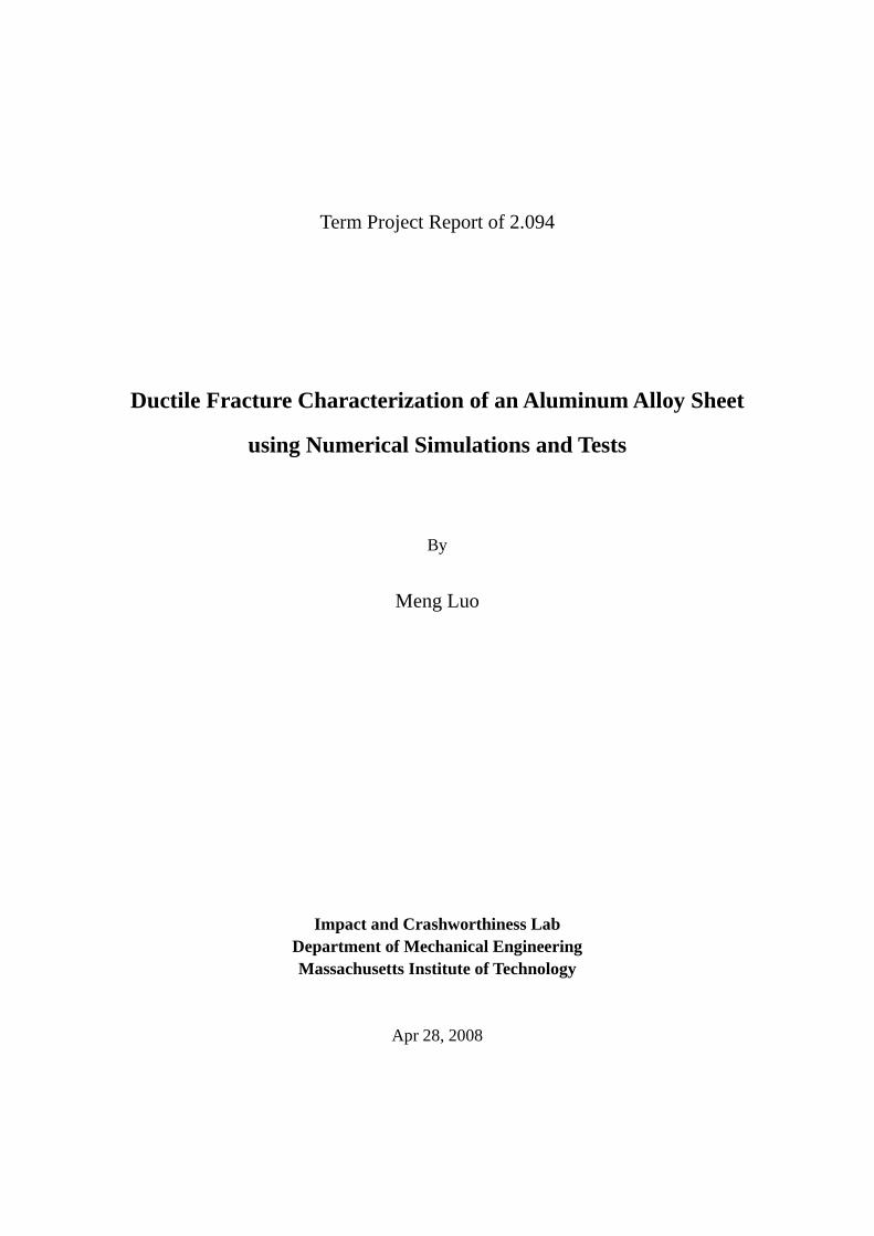
of the dog-bone tension tests were built in ADINA two with 4-node shell elements the other two with 8-node solid elements For each element type both isotropic and orthotropic plasticity model were used Since the specimen is symmetric with respect to all three axes only a 18 model was built with solid elements and a quarter model was built with shell elements The top of the specimen is subjected to a prescribed displacement and symmetric boundary conditions are set on corresponding edges (lines for shell surfaces for solid elements) The models are shown in figure 2-8~2-11
The elastic material parameters used in the models areE=69Gpa density=2700kgm3 poisson ratio=033 The plastic stress strain curve used for both isotropic and orthotropic material model is the one in Fig 2-6 The lankford parameters for orthotropic material model are shown in table 2-1 Since the aluminum sheet is almost planar isotropic and our objective is to investigate the difference between orthotropic and isotropic material model the material a direction (rolling direction) was simply set to along with the tension direction for orthotropic material model (Fig 2-9 2-11) The mesh edge length is about 1mm and the number of though thickness integration points is set to 5 for shell model
Fig 2-8 Model 1 Shell element with isotropic material model
Fig 2-9 Model 2Shell element with orthotropic material model
Fig 2-10 Model 3 Solid element with isotropic material model
Fig 2-11 Model 4 Solid element with orthotropic material model
No 5 Total 21
Term Project Report of 2094
To obtain the force-displacement response a time function is defined for the prescribed displacement and the time step is 001s The analysis assumptions are large displacement and strain and a full Newton method was used for iteration All the models are run in the environment of ADINA statics hereafter in this report
Fig 2-3 shows that the average gauge section elongation to fracture is 61mm The corresponding deformation shape and effective plastic strain band plot at the fracture point are shown in Fig 2-12~2-15 The deformation figures shows that only model 3 which is with isotropic material model and solid elements can predict the necking phenomenon before fracture see Fig 216
Fig 2-12 Deformation and strain output of model 1 Fig 2-13 Deformation and strain output of model 2
Fig 2-14 Deformation and strain output of model 3 Fig 2-15 Deformation and strain output of model 4
Fig 2-16 Necking occurs in tensile tests From the simulation result the total reaction force of the top nodes and the gauge
No 6 Total 21
Term Project Report of 2094
nodes displacement can be obtained The load displacement responses and the experimental results were compared in Fig 2-17 Apparently the model 3 result accords with experimental result very well
Load
(kN
) 12
10
8
6
4
2
0
Test Result Model1Shell+Isotropy Model2Shell+Orthotropy Model3Solid+Isotropy Model4Solid+Orthotropy
00 05 10 15 20 25 30 35 40 45 50 55 60 65 70
Elongation (mm)
Fig 2-17 Comparison of load-displacement curves between experiment and simulations Previous research of ICL shows that the crack initiates at the center of the dog-bone
specimen in a tensile test Therefore the equivalent plastic strains of the central element at the fracture elongation point obtained from the numerical models were summarized in table 2-2 and compared with the fracture strain measure from thickness and width reduction of specimens (low precision) Again model 3 gives the best prediction of the local equivalent strain to fracture Hence one can conclude that the model with solid elements and isotropic plasticity model can give accurate numerical prediction for the dog-bone specimen tensile tests The reason why the shell element can not give good prediction might be that the width thickness ratio of the specimen cross-section is not big enough for a shell assumption
One can also obtain the stress triaxiality information (negative pressure divided by effective stress) of the central point of the specimen from numerical simulation The evolution of stress triaxiality with the elongation of the gauge section is shown in Fig 2-18 The average triaxiality value up to fracture is about 0345 and the triaxiality before necking is exactly equal to the analytical value 13 The average stress triaxiality would be used for fracture calibration together with the fracture strain Table 2-2 Comparison of equivalent strain to fracture of dog-bone specimen between simulations and
test of dog-bone specimens
Model 1 Model 2 Model 3 Model 4 Measurement after test
Fracture strain 012 013 048 010 053
No 7 Total 21
Term Project Report of 2094
Stre
ss T
riaxi
ality
045
044
043
042
041
040
039
038
037
036
035
034
033
032 Fracture 031
030 00 05 10 15 20 25 30 35 40 45 50 55 60 65
Elongation (mm)
Fig 2-18 Evolution of stress triaxiality calculated by ADINA
22 Flat specimen with cutouts The flat specimen with cutouts was used to obtain additional point for the calibration
of the ductile fracture model of our aluminum sheets The geometry of the specimen is shown in Fig 2-19 The initial stress triaxiality in a tensile test of this specimen can be easily controlled by changing the diameter of the cutout contour The geometry of the specimens in this project gives an analytical initial triaxiality of 052 Two FE models were set up in ADINA with 4-node shell elements and 8-node solid elements respectively With the symmetric conditions one only need to build a 14 model of the gauge section with shell elements and a 18 model of the gauge section with solid elements Fig 2-20 and Fig 2-21 shows the deformation and equivalent plastic strain contour of these two models at the fracture elongation point
Based on the studies in section 21 only isotropic material model was used for the simulations hereafter and the true stress strain curve in Fig 2-6 was adopted The mesh edge length of both models is 1mm 5 through thickness Gauss integration points were used in the shell element model The effect of the through thickness integration point number will be discussed in section 3
Fig 2-19 Geometry of flat specimen with cutouts
No 8 Total 21
Term Project Report of 2094
Fig 2-20 Deformation and strain output at fracture Fig 2-21 Deformation and strain output at fracture elongation point of shell element model elongation point of solid element model The load displacement responses and the experimental results were compared in Fig
2-22 Apparently the shell element model result correlates with experimental result better For this specimen crack also initiate at the center point of the specimen so the equivalent plastic strains to fracture of the central elements of the two models were obtained from the ADINA models and are shown in table 2-3 together with the fracture strain measured after test The shell element model gives a better prediction of equivalent strain to fracture than the solid element model
Load
(kN
)
14
12
10
8
6
4
2
0
Test Result Solid element model Shell element model
00 01 02 03 04 05 06 07 08 09 10 11 12 13
Elongation(mm)
Fig 2-22 Comparison of the load-elongation curves between FE models and test Table 2-3 Comparison of equivalent strain to fracture between simulations and test
Shell Model Solid Model Test Measurement Fracture strain 021 013 025
The evolution of stress triaxiality with the elongation of the gauge section of this specimen calculated by the shell element model is shown in Fig 2-23 The average triaxiality value up to fracture is about 051 and very close to the analytical value 052 The average stress triaxiality would be used for fracture calibration together with the fracture strain
No 9 Total 21
Term Project Report of 2094
Stre
ss T
riaxi
ality
060
055
050
045 02 04 06 08 10 12 14
Elongation(mm)
Fig 2-23 Evolution of stress triaxility of the flat specimen with cutouts
23 Flat grooved plane strain specimen Another type of specimen for the fracture calibration tests is the flat grooved
specimen which can provide a plane strain condition in the uniaxial tensile test The geometry of the specimen and a tested specimen is shown in Fig 2-24 Two FE models were set up in ADINA with 4-node plane strain elements and 8-node solid elements respectively With the symmetric conditions one only need to build a 14 model of the gauge section with plane strain elements and a 18 model of the gauge section with solid elements Fig 2-25 and Fig 2-26 show the two models
The load displacement responses and the experimental results were compared in Fig 2-27 For this specimen crack also initiate at the center point of the specimen so the equivalent plastic strains to fracture of the central elements of the two models were obtained from the ADINA models and are shown in table 2-4 together with the fracture strain measured after test using digital image correlation method
(a) Geometry of flat grooved specimen (b)A tested specimen Fig 2-24
No 10 Total 21
Term Project Report of 2094
Fig 2-25 Plane strain element model Fig 2-26 Solid element model
20 19 Test result18 Plane strain element model17
Solid element model 16 15 14 13 12 11 10 9 8 7 6 5 4 3 2 1 0000 005 010 015 020 025 030 035 040 045 050 055 060
Elongation(mm)
Load
(kN
)
Fig 2-27 Comparison of the load-elongation curves between FE models and test of plane strain specimen
Table 2-4 Comparison of equivalent strain to fracture of plane strain specimen
Plane Strain Model Solid Model Test Measurement Fracture strain 0139 0138 020
From Fig 2-27 and table 2-4 one can see that plane strain element and solid element model give almost identical prediction of load-displacement response and local strain at the center point of the specimen However using plane strain elements can greatly reduce the number of elements and thus save CPU time Fig 2-28 demonstrate that the strain in x direction is almost zero so the plane strain element is good enough to modeling tension test of this specimen
The evolution of stress triaxialities with the elongation of the gauge section of the plane strain specimen calculated by two models are shown in Fig 2-29 The average triaxiality value up to fracture is about 0572 and very close to the analytical value 0577 The average stress triaxiality would be used for fracture calibration together with the fracture strain
No 11 Total 21
Term Project Report of 2094
Fig 2-28 The band plot of the strain in XX direction
Plane strain element model
Stre
ss T
riaxi
ality
060
056
052
048
Solid element model
Fracture
01 02 03 04 05 06
Elongation(mm)
Fig 2-29 Evolution of stress triaxility of the flat grooved plane strain specimen
24 Punch indentation tests on circular disks This test provides information on fraction under the equi-biaxial state of stress
The most highly stressed point is located at the apex of the dome where the components of radial and circumferential stress and strain are equal to each other The disk specimens were secured to the 100mm diameter die by a heavy flange with 8 bolts The radius of the hemi-spherical punch was 45mm The load-displacement characteristics were recorded in the tests The measured displacement to fracture in our case was 274mm The tests were interrupted right after formation of nearly straight crack shown as shown in Fig 2-30
Accordingly a FE model of this test was built in ADINA with 4-node axisymmetric elements which is shown in Fig 2-31 The mesh edge length is 1mm The edge nodes of the disk model were fixed at all degree of freedom the center nodes of the disk model were given a symmetric boundary condition and the punch surface was given a prescribed downward displacement The contact surface on the punch was modeled as rigid and the friction coefficient is set to 001 The pressuredisplacement mixed interpolation function was used for this model to get better stress triaxiality prediction the difference between displacement-based and up mixed element will be discussed in
No 12 Total 21
Term Project Report of 2094
section 3 The time step was set to 0005s The deformation and the effective strain distribution of the disk were shown in Fig 2-32
Fig 2-30 A view of the fractured disk Fig 2-31 Numerical model of the punch test
Fig 2-32 Deformation and distribution of the disk specimen calculated by ADINA
The force displacement response can be obtained by plotting the reaction force on the punch and the displacement of the punch The comparison of the force displacement response between simulation and test result is shown in Fig 2-33 There is an excellent agreement of the measured load-displacement curve with the numerical model Also the history of the effective strain and stress triaxiality of the outer element at the apex of the dome was shown in Fig 2-34 from which one can obtain the equivalent strain to fracture of this specimen and the average stress triaxiality up to fracture of the fracture initiation point (apex of the dome) For the case of our aluminum sheet the calculated fracture strain is 063 which is very close to the strain value 069 from the measurement of thickness reduction after test The average triaxiality value up to fracture is about 065 and very close to the analytical value 23 The average stress triaxiality would be used for
No 13 Total 21
Term Project Report of 2094
fracture calibration together with the fracture strain 063
100
Forc
e(kN
)
90
80
70
60
50
40
30
20
10
0
Test result Numerical simulation
0 5 10 15 20 25 30 35
Displacement(mm)
Fig2-33 Comparison of the force displacement response of a punch test between test result and simulation output
00
02
04
06
08
10
12
14
16
18
20
Stre
ss T
riaxi
ality
Equi
vale
nt P
last
ic S
train
Equivalent plstic strain Stress triaxiality
Fracture
0 2 4 6 8 10 12 14 16 18 20 22 24 26 28 30 32 34 36 38 40
Displacement (mm)
Fig 2-34 Evolution of equivalent plastic strain and stress triaxiality at the fracture initiation point
25 Ductile fracture calibration using simulation results As all the numerical simulations of calibration tests has been performed and validated
by experimental results a fracture locus of our aluminum sheets can be calibrated with the simulation results Table 2-5 shows all the fracture points obtained from the numerical simulation
Table 2-5 Fracture points obtained from numerical simulations Point Specimen Type Stress Triaxiality Fracture Strain
1 Dog-bone 0345 048 2 Flat with cutouts 051 021 3 Flat grooved 0572 014 4 Punch indentation 065 063
No 14 Total 21
Term Project Report of 2094
A Mohr-Coulomb fracture criterion was used to calibrate the fracture locus of this aluminum sheet The form of this fracture criterion in the space of fracture strain and stress triaxiality is as followed
minus1
ε f = ⎨⎪⎧
⎪⎩cA 2
f3 ⎢⎡
⎣⎢⎜⎛
⎝⎜
1+ 3 c1
2
sdot f1 ⎟⎞⎟⎠+ c1
⎛⎜⎝η +
f 3
2 ⎞⎟⎠⎥⎤
⎥⎦
⎪⎬⎫
⎭⎪
n
(2-3)
where the functions f1 f2 and f3 are defined as
f1 1 27 η η 2 = cos arcsin ⎢
⎡minus ( minus 1)⎤⎥3 ⎣ 2 3 ⎦
( 2f2 = sin 1 arcsin ⎡minus 27 η η minus 1)⎤ (2-4) 3 ⎣⎢ 2 3 ⎥⎦
f3 c3 3 (1minus c3)( 1 minus1)= +
2 minus 3 f1
This fracture criterion is a function of equivalent strain to fracture ε f in terms of the
average stress triaxiality η up to fracture A and n are the material parameters in Eq
(2-1) This criterion has 3 calibration parameters c1c2 and c3 Hence points 1 3 and 4 in table 2-5 were used to calibrate the 3 free parameters while point 2 was used to validate the accuracy of the fracture locus The calibrated fracture locus is shown in Fig 2-35 One can see that the calibrated fracture locus can predict the fracture strain at point 2 (flat specimen with side cutouts) with good accuracy Therefore this fracture locus can be implemented into the FE codes to predict ductile fracture during calculations
c1=0154 c2=248MPa c3=098 A=438MPa n=007
Calibration Points
Validation Point
Fig2-35 Calibrated fracture locus of our aluminum sheets with numerical results
No 15 Total 21
Term Project Report of 2094
3 Parametric Study of Some Numerical Simulation Parameters To predict the initial crack position accurately the local strain and stress triaxiality are
very important to the fracture identification However some parameters may affect the local strainstress significantly such as number of integration points (NIP) through thickness element type mesh size and so on
Several finite element models were built based on the benchmark models in section 2 to study these effects The force-displacement response effective strain and stress triaxilality history at the initial crack position were compared and analyzed
31 Effect of Number of Integration Point through thickness (NIP) This study is based on the shell element model of the flat specimen with cutouts The
benchmark model in section 22 is with 5 integration points though thickness and the Gauss integration was used Two more shell element models of the flat specimen with cutouts with 2 and 3 through thickness integration points respectively were built in ADINA
As is shown in Fig 3-1 as the NIP through thickness of shell elements increases the load-elongation response predicted by the numerical model is closer to the experimental results From Fig 3-2 and 3-3 one can see that the local strain and stress triaxiality at the crack initiation point (the center of the specimen) predicted by the 2 NIP model are much lower than the 5 NIP model which has shown good accuracy in section 22 Hence if shell elements are used for numerical simulations of similar problems at least 5 through thickness integration points should be employed
Load
(kN
)
17 16 15 14 13 12 11 10 9 8 7 6 5 4 3 2 1 0
Test INP=2 INP=3 INP=5
Fracture
00 01 02 03 04 05 06 07 08 09 10 11 12 13 14 15
Elongation(mm)
Fig 3-1 Load-elongation responses of three models with different NIP through thickness
No 16 Total 21
Term Project Report of 2094
Equ
ival
ent P
last
ic S
train
10
09
08
07
06
05
04
03
02
01
00
INP=2 INP=3 INP=5
Fracture
00 02 04 06 08 10 12 14 16 18 20
Elongation(mm)
Fig 3-2 Strain history at crack initiation point of three models with different NIP through thickness
044
046
048
050
052
054
056
058
Stre
ss T
riaxi
ality
NIP=2 NIP=3 NIP=5
Fracture
02 04 06 08 10 12 14
Elongation(mm)
Fig 3-3 Stress triaxiality history at crack initiation point of three models with different NIP through thickness
32 Effect of element type This study is based on the model of punch indentation tests in section 24 Three
different models with different element types and interpolation formulations were
No 17 Total 21
Term Project Report of 2094
compared in this section displacement based 4-node element mixed 41 and 93 up element
From Fig3-4 and Fig 3-5 one can see that the force-displacement response and local strain evolution at the crack initiation point (the apex of the dome) are not affected much by the element type However as is shown in Fig 3-6 the displacement based element can not predict the stress triaxiality well because the analytical stress triaxiality value should be 23 in this test Since stress triaxiality is a normalized pressure the low accuracy triaxiality prediction is due to the unreasonable pressure distribution and magnitudes predicted by the displacement-based elements as is shown in Fig 3-7 The pressure distribution calculated by mixed up elements are much more accurate as is shown in Fig 3-8
Test 4-node displacement based element 41 mixed up element 93 mixed up element
Fracture
0 5 10 15 20 25 30 35 40 45 50
Displacement(mm)
Equ
ival
ent P
last
ic S
train
07
06
05
04
03
02
01
0 2 4 6 8 10 12 14 16 18 20 22 24 26 28
4-node displacement based element 41 mixed up element 93 mixed up element
Fracture
120
110
100
90
80
Forc
e(kN
)
70
60
50
40
30
20
10
0 00
Displacement(mm)
Fig 3-4 Force-displacement responses of 3 models Fig 3-5 Equivalent plastic strain evolution at crack with different element types initiation point of 3 models with different element
types
10
05
00
4-node displacment based elment 41 mixed up element 93 mixed up element
-05
-10
-15
-20
-25
-30
-35
-40
-45
-50
Stre
ss T
riaxi
ality
0 5 10 15 20 25 30
Displacement(mm)
Fig 3-6 Evolution of stress triaxiality at crack initiation point of 3 element types
No 18 Total 21
Term Project Report of 2094
Fig 3-7 Pressure distribution of the model with 4 node Fig 3-8 Pressure distribution of the model with 93 displacement based elments mixed elements
33 Mesh size effect This study is based on the model of punch indentation tests in section 24 Three
different models with different mesh sizes were built as is shown in Fig 3-9 and the force-displacement responses local strain and stress triaxiality history at the crach initiation point (the apex of the dome) were compared and studied The 3 different mesh edge length studied in this section was 1mm 05mm and 2mm The 41 mixed up elements were employed in all three models
Fig 3-10 and 3-11 show that the force-displacement response and stress triaxiality predicted by the numerical models become closer to the experimental result or analytical result as the mesh goes finer As is shown by Fig 3-12 the local strain seems to be larger as the mesh edge length is smaller in the early stage but it reach convergence finally Hence the finite element model is convergent as the mesh becomes finer
(a)Mesh edge length=1mm (b)Mesh edge length=05mm (c)Mesh edge length=2mm Fig 3-9 Three models with different mesh size
No 19 Total 21
Term Project Report of 2094
Test Mesh edge length=1mm 08
Mesh edge length=1mm Mesh edge length=2mm Mesh edge length=05mm
Mesh edge length=05mm Mesh edge length=2mm
120
110
100
07
06 90
80
Stre
ss T
riaxi
ality
05
04
03 Forc
e(kN
)
70
60
50
40
30
20
02
01
00
10
0 0 5 10 15 20 25 30 35 40 45 50 0 5 10 15 20 25 30 35 40 45 50
Displacement(mm) Displacement(mm)
Fig 3-10 Force-displacement responses of 3 models Fig 3-11 Evolution of stress triaxiality at crack with different element size initiation point of 3 models with different element size
10
Mesh edge length=1mm 08 Mesh edge length=05mm Mesh edge length=2mm
Equi
vale
nt P
lstic
Stra
in
06
04
02
00 0 5 10 15 20 25 30
Displacement(mm)
Fig 3-12 Equivalent plastic strain evolution at crack initiation point of 3 models with different element size
No 20 Total 21
Term Project Report of 2094
4 Conclusions In this project four types of specimens made from our aluminum sheets were tested
in the lab to investigate the fracture characteristics of this material At the same time corresponding finite element models were built to simulate the fracture calibration tests Most suited model for each test was determined after comparisons and analysis and the fracture locus of this material was calibrated with the simulation results Moreover a brief parametric study was performed to evaluate the effect of several FE parameters on the numerical simulation results Main conclusions are shown as followed
1) Finite element model can simulate the physical problems very well Suited FE models can predict the load-displacement responses local strain and stress with good accuracy
2) Selection of element type and modeling strategy should depend on the geometry and boundary conditions of the physical problem For this project one should choose solid elements for dog-bone specimen shell elements for flat specimen with cutouts plane strain elements for flat grooved specimen and axisymmetric elements for the punch indentation test
3) Number of integration points (NIP) through thickness has a great effect on the strain and stress distribution of shell elements Once the through thickness stress gradient is involved in a physical problem such as necking or bending a larger NIP through thickness should be employed
4) The up mixed element can predict the pressure distribution and magnitude much more accurate
5) The FE models in this project are convergent As the mesh becomes finer both the load-displacement response and local stressstrain output become closer to experimental results or analytical values
No 21 Total 21
MIT OpenCourseWare httpocwmitedu
2094 Finite Element Analysis of Solids and Fluids IISpring 2011
For information about citing these materials or our Terms of Use visit httpocwmiteduterms

Term Project Report of 2094
Contents
Abstract 1
1 Introduction1
2 Numerical Simulations of Four Fracture Calibration Test2
21 Dog-bone tensile sepcimens 2
22 Flat specimen with cutouts 8
23 Flat grooved plane strain specimen 10
24 Punch indentation tests on circular disks 12
25 Ductile fracture calibration using simulation results 14
3 Parametric Study of Some Numerical Simulation Parameters 16
31 Effect of Number of Integration Point through thickness (NIP) 16
32 Effect of element type 17
33 Mesh size effect 19
4 Conclusions21
I
Term Project Report of 2094
Abstract The objective of this project is to characterize the plastic behavior and ductile fracture
of the 2mm-thick aluminum alloy sheets Four different types of tests were conducted all the way to fracture including tensile tests on classical dog-bone specimens flat specimens with cutouts and plane strain grooved specimens as well as a punch indentation test A comprehensive numerical analysis of these experiments was performed with ADINA Simulations revealed that the isotropic plasticity model is able to describe with good accuracy the plastic response of all four types of tests Moreover local equivalent strain to fracture and stress triaxiality parameters were obtained through FE simulations using an inverse engineering method and a fracture locus of this type of aluminum alloy sheets was determined In addition a parametric study was performed to evaluate the effect some variables that will affect numerical simulations such as number of integration points through thickness element type and mesh size
1 Introduction Prediction of ductile fractures of metals in engineering structures is a topic of great
importance in the automotive aerospace and military industries Equivalent strain to
fracture ε f (or the fracture strain for short) is widely used to define the material ductility
Many theoretical analyses and experimental results have shown that the materialrsquos fracture strain is not constant but changes under different loading conditions or stress states The most important fracture controlling parameter is the stress triaxiality η (normalized hydrostatic pressure by Mises equivalent stress σ
= minus p )m
σ σ
Based on the research experience of ICL(Impact and Crashworthiness Lab) at MIT a
Mohr-Coulomb fracture criterion in the space of ε f and η was adopted in this project
to determine the fracture locus of the aluminum sheets For sheet metal the stress
triaxiality range of most interest is 1 3 ltη lt 2 3 Therefore four types of tests which
can cover this range were designed to calibrate the fracture model The present approaches include experimental study and FE simulation Experiments
will provide the load-displacement response the location and position of fracture initiation FE simulations are used to calculate all the stress states and strain components at the point of fracture initiation
Besides the fracture calibration a parametric study based on the ADINA simulations of the calibration tests was conducted to evaluate the effect of several important finite element parameters
No 1 Total 21
Term Project Report of 2094
2 Numerical Simulations of Four Fracture Calibration Test Four different types of tests which can cover different stress triaxialities were
conducted on a MTS uniaxial testing machine All four types of specimens were cut from the 2mm-thick aluminum sheet The analytical triaxialities for the four types of tests are 13(dog-bone specimen) 052(flat specimen with cutout) 0577(plane strain specimen) and 23(punch indentation) Corresponding numerical simulations were performed to predict to load displacement responses and obtain local stress states and strain components All the numerical simulations of this project were run in the environment of ADINA V844 and within ADINA structures and statics
Fig 2-1 MTS testing machine
21 Dog-bone tensile specimens 211 Obtaining hardening rule and quantification of anisotropy
Uniaixal tensile tests on the dog-bone specimens cut from the aluminum sheets are very important since the material data needed for the FE simulations are usually obtained by these tests Nine dog-bone specimens were cut using water-jet machining three from each of the following directions (angle between the tensile direction and the material rolling direction) 0o 45o and 90o as is shown in Fig 2-2
Fig 2-2 Original sheet of from which specimens were machined
No 2 Total 21
Term Project Report of 2094
Force versus displacement was recorded during each of the 12 uniaxial tension tests The recorded force-displacement data in three directions is shown in Fig 2-3 The onset of diffuse necking is indicated for each test The calculated engineering stress-strain curve up to necking is given in Fig 2-4
It is clear that the load-displacement curves are the same in all three directions up to the point of necking This means that sheets exhibit planar anisotropy The corresponding true stress versus the equivalent plastic strain up to the necking strain is shown in Fig 2-5
In order to extend the range of strain and avoid tensile instability a simple power law fitting of the true stress strain curve was used in this project Comparison of the true stress-true strain curves with the power law fit is shown in Fig 2-6 The form of the power law fitting is
σ = A e )n (2-1) ( 0 +ε p
Using least square method the parameters of the power law fitting are
A = 438MPa e0 = 000434 n = 007
Fig 2-3 Force versus displacement curves measured for dog-bone specimens
Fig 2-4 Engineering stress strain curves up to necking for dog-bone specimens
Fig 2-5 True stress versus plastic strain calculated Fig 2-6 True stress-strain curve obtained from up to necking for dog-bone specimen uniaxial dog-bone specimen tension tests and the power
tension tests hardening fit
No 3 Total 21
ε11
ε22
Term Project Report of 2094
The true stress strain relation in Fig 2-6 can be used for the material input of ADINA However aluminum sheets are known to develop considerable anisotropy during the extrusion and rolling processes and subsequent heat treatment Although Fig 2-3~2-5 indicate that this sheet are planar anisotropic one still need to quantify the anisotropy of this material especially the transverse (through thickness) anisotropy Since the plastic orthotropic material in ADINA is a good choice to represent the transverse anisotropic material several measurements were taken to obtain the Lankford parameter needed for the orthotropic material model
This parameter referred to as ldquo rα rdquo is the ratio of the strain in the width
direction dεα+π 2 to the strain through the thickness direction dε 3 of a specimen
subjected to uniaxial tension in the direction defined by the angle α measured from the rolling direction
dεα+π 2 rα = (2-2) dε 3
The Lankford parameter in three directions was measured using Digital Image Correlation as shown in Fig 2-7 The calculated values of the Lankford parameters are given in Table 2-1 Herein all the material data needed for both the isotropic and an orthotropic material model in ADINA have been obtained from tests
ε11
ε22
Fig 2-7 Measuring lankford parameters with Digital image correlation
Table 2-1 Measured value of the Lankford parameters for our aluminum sheet
r0 = rx r45 r90 = ry
0638 06 07
No 4 Total 21
Term Project Report of 2094
212 Numerical simulations of dog-bone specimen tensile test In order to find the best numerical model for the series of tests total four FE models
of the dog-bone tension tests were built in ADINA two with 4-node shell elements the other two with 8-node solid elements For each element type both isotropic and orthotropic plasticity model were used Since the specimen is symmetric with respect to all three axes only a 18 model was built with solid elements and a quarter model was built with shell elements The top of the specimen is subjected to a prescribed displacement and symmetric boundary conditions are set on corresponding edges (lines for shell surfaces for solid elements) The models are shown in figure 2-8~2-11
The elastic material parameters used in the models areE=69Gpa density=2700kgm3 poisson ratio=033 The plastic stress strain curve used for both isotropic and orthotropic material model is the one in Fig 2-6 The lankford parameters for orthotropic material model are shown in table 2-1 Since the aluminum sheet is almost planar isotropic and our objective is to investigate the difference between orthotropic and isotropic material model the material a direction (rolling direction) was simply set to along with the tension direction for orthotropic material model (Fig 2-9 2-11) The mesh edge length is about 1mm and the number of though thickness integration points is set to 5 for shell model
Fig 2-8 Model 1 Shell element with isotropic material model
Fig 2-9 Model 2Shell element with orthotropic material model
Fig 2-10 Model 3 Solid element with isotropic material model
Fig 2-11 Model 4 Solid element with orthotropic material model
No 5 Total 21
Term Project Report of 2094
To obtain the force-displacement response a time function is defined for the prescribed displacement and the time step is 001s The analysis assumptions are large displacement and strain and a full Newton method was used for iteration All the models are run in the environment of ADINA statics hereafter in this report
Fig 2-3 shows that the average gauge section elongation to fracture is 61mm The corresponding deformation shape and effective plastic strain band plot at the fracture point are shown in Fig 2-12~2-15 The deformation figures shows that only model 3 which is with isotropic material model and solid elements can predict the necking phenomenon before fracture see Fig 216
Fig 2-12 Deformation and strain output of model 1 Fig 2-13 Deformation and strain output of model 2
Fig 2-14 Deformation and strain output of model 3 Fig 2-15 Deformation and strain output of model 4
Fig 2-16 Necking occurs in tensile tests From the simulation result the total reaction force of the top nodes and the gauge
No 6 Total 21
Term Project Report of 2094
nodes displacement can be obtained The load displacement responses and the experimental results were compared in Fig 2-17 Apparently the model 3 result accords with experimental result very well
Load
(kN
) 12
10
8
6
4
2
0
Test Result Model1Shell+Isotropy Model2Shell+Orthotropy Model3Solid+Isotropy Model4Solid+Orthotropy
00 05 10 15 20 25 30 35 40 45 50 55 60 65 70
Elongation (mm)
Fig 2-17 Comparison of load-displacement curves between experiment and simulations Previous research of ICL shows that the crack initiates at the center of the dog-bone
specimen in a tensile test Therefore the equivalent plastic strains of the central element at the fracture elongation point obtained from the numerical models were summarized in table 2-2 and compared with the fracture strain measure from thickness and width reduction of specimens (low precision) Again model 3 gives the best prediction of the local equivalent strain to fracture Hence one can conclude that the model with solid elements and isotropic plasticity model can give accurate numerical prediction for the dog-bone specimen tensile tests The reason why the shell element can not give good prediction might be that the width thickness ratio of the specimen cross-section is not big enough for a shell assumption
One can also obtain the stress triaxiality information (negative pressure divided by effective stress) of the central point of the specimen from numerical simulation The evolution of stress triaxiality with the elongation of the gauge section is shown in Fig 2-18 The average triaxiality value up to fracture is about 0345 and the triaxiality before necking is exactly equal to the analytical value 13 The average stress triaxiality would be used for fracture calibration together with the fracture strain Table 2-2 Comparison of equivalent strain to fracture of dog-bone specimen between simulations and
test of dog-bone specimens
Model 1 Model 2 Model 3 Model 4 Measurement after test
Fracture strain 012 013 048 010 053
No 7 Total 21
Term Project Report of 2094
Stre
ss T
riaxi
ality
045
044
043
042
041
040
039
038
037
036
035
034
033
032 Fracture 031
030 00 05 10 15 20 25 30 35 40 45 50 55 60 65
Elongation (mm)
Fig 2-18 Evolution of stress triaxiality calculated by ADINA
22 Flat specimen with cutouts The flat specimen with cutouts was used to obtain additional point for the calibration
of the ductile fracture model of our aluminum sheets The geometry of the specimen is shown in Fig 2-19 The initial stress triaxiality in a tensile test of this specimen can be easily controlled by changing the diameter of the cutout contour The geometry of the specimens in this project gives an analytical initial triaxiality of 052 Two FE models were set up in ADINA with 4-node shell elements and 8-node solid elements respectively With the symmetric conditions one only need to build a 14 model of the gauge section with shell elements and a 18 model of the gauge section with solid elements Fig 2-20 and Fig 2-21 shows the deformation and equivalent plastic strain contour of these two models at the fracture elongation point
Based on the studies in section 21 only isotropic material model was used for the simulations hereafter and the true stress strain curve in Fig 2-6 was adopted The mesh edge length of both models is 1mm 5 through thickness Gauss integration points were used in the shell element model The effect of the through thickness integration point number will be discussed in section 3
Fig 2-19 Geometry of flat specimen with cutouts
No 8 Total 21
Term Project Report of 2094
Fig 2-20 Deformation and strain output at fracture Fig 2-21 Deformation and strain output at fracture elongation point of shell element model elongation point of solid element model The load displacement responses and the experimental results were compared in Fig
2-22 Apparently the shell element model result correlates with experimental result better For this specimen crack also initiate at the center point of the specimen so the equivalent plastic strains to fracture of the central elements of the two models were obtained from the ADINA models and are shown in table 2-3 together with the fracture strain measured after test The shell element model gives a better prediction of equivalent strain to fracture than the solid element model
Load
(kN
)
14
12
10
8
6
4
2
0
Test Result Solid element model Shell element model
00 01 02 03 04 05 06 07 08 09 10 11 12 13
Elongation(mm)
Fig 2-22 Comparison of the load-elongation curves between FE models and test Table 2-3 Comparison of equivalent strain to fracture between simulations and test
Shell Model Solid Model Test Measurement Fracture strain 021 013 025
The evolution of stress triaxiality with the elongation of the gauge section of this specimen calculated by the shell element model is shown in Fig 2-23 The average triaxiality value up to fracture is about 051 and very close to the analytical value 052 The average stress triaxiality would be used for fracture calibration together with the fracture strain
No 9 Total 21
Term Project Report of 2094
Stre
ss T
riaxi
ality
060
055
050
045 02 04 06 08 10 12 14
Elongation(mm)
Fig 2-23 Evolution of stress triaxility of the flat specimen with cutouts
23 Flat grooved plane strain specimen Another type of specimen for the fracture calibration tests is the flat grooved
specimen which can provide a plane strain condition in the uniaxial tensile test The geometry of the specimen and a tested specimen is shown in Fig 2-24 Two FE models were set up in ADINA with 4-node plane strain elements and 8-node solid elements respectively With the symmetric conditions one only need to build a 14 model of the gauge section with plane strain elements and a 18 model of the gauge section with solid elements Fig 2-25 and Fig 2-26 show the two models
The load displacement responses and the experimental results were compared in Fig 2-27 For this specimen crack also initiate at the center point of the specimen so the equivalent plastic strains to fracture of the central elements of the two models were obtained from the ADINA models and are shown in table 2-4 together with the fracture strain measured after test using digital image correlation method
(a) Geometry of flat grooved specimen (b)A tested specimen Fig 2-24
No 10 Total 21
Term Project Report of 2094
Fig 2-25 Plane strain element model Fig 2-26 Solid element model
20 19 Test result18 Plane strain element model17
Solid element model 16 15 14 13 12 11 10 9 8 7 6 5 4 3 2 1 0000 005 010 015 020 025 030 035 040 045 050 055 060
Elongation(mm)
Load
(kN
)
Fig 2-27 Comparison of the load-elongation curves between FE models and test of plane strain specimen
Table 2-4 Comparison of equivalent strain to fracture of plane strain specimen
Plane Strain Model Solid Model Test Measurement Fracture strain 0139 0138 020
From Fig 2-27 and table 2-4 one can see that plane strain element and solid element model give almost identical prediction of load-displacement response and local strain at the center point of the specimen However using plane strain elements can greatly reduce the number of elements and thus save CPU time Fig 2-28 demonstrate that the strain in x direction is almost zero so the plane strain element is good enough to modeling tension test of this specimen
The evolution of stress triaxialities with the elongation of the gauge section of the plane strain specimen calculated by two models are shown in Fig 2-29 The average triaxiality value up to fracture is about 0572 and very close to the analytical value 0577 The average stress triaxiality would be used for fracture calibration together with the fracture strain
No 11 Total 21
Term Project Report of 2094
Fig 2-28 The band plot of the strain in XX direction
Plane strain element model
Stre
ss T
riaxi
ality
060
056
052
048
Solid element model
Fracture
01 02 03 04 05 06
Elongation(mm)
Fig 2-29 Evolution of stress triaxility of the flat grooved plane strain specimen
24 Punch indentation tests on circular disks This test provides information on fraction under the equi-biaxial state of stress
The most highly stressed point is located at the apex of the dome where the components of radial and circumferential stress and strain are equal to each other The disk specimens were secured to the 100mm diameter die by a heavy flange with 8 bolts The radius of the hemi-spherical punch was 45mm The load-displacement characteristics were recorded in the tests The measured displacement to fracture in our case was 274mm The tests were interrupted right after formation of nearly straight crack shown as shown in Fig 2-30
Accordingly a FE model of this test was built in ADINA with 4-node axisymmetric elements which is shown in Fig 2-31 The mesh edge length is 1mm The edge nodes of the disk model were fixed at all degree of freedom the center nodes of the disk model were given a symmetric boundary condition and the punch surface was given a prescribed downward displacement The contact surface on the punch was modeled as rigid and the friction coefficient is set to 001 The pressuredisplacement mixed interpolation function was used for this model to get better stress triaxiality prediction the difference between displacement-based and up mixed element will be discussed in
No 12 Total 21
Term Project Report of 2094
section 3 The time step was set to 0005s The deformation and the effective strain distribution of the disk were shown in Fig 2-32
Fig 2-30 A view of the fractured disk Fig 2-31 Numerical model of the punch test
Fig 2-32 Deformation and distribution of the disk specimen calculated by ADINA
The force displacement response can be obtained by plotting the reaction force on the punch and the displacement of the punch The comparison of the force displacement response between simulation and test result is shown in Fig 2-33 There is an excellent agreement of the measured load-displacement curve with the numerical model Also the history of the effective strain and stress triaxiality of the outer element at the apex of the dome was shown in Fig 2-34 from which one can obtain the equivalent strain to fracture of this specimen and the average stress triaxiality up to fracture of the fracture initiation point (apex of the dome) For the case of our aluminum sheet the calculated fracture strain is 063 which is very close to the strain value 069 from the measurement of thickness reduction after test The average triaxiality value up to fracture is about 065 and very close to the analytical value 23 The average stress triaxiality would be used for
No 13 Total 21
Term Project Report of 2094
fracture calibration together with the fracture strain 063
100
Forc
e(kN
)
90
80
70
60
50
40
30
20
10
0
Test result Numerical simulation
0 5 10 15 20 25 30 35
Displacement(mm)
Fig2-33 Comparison of the force displacement response of a punch test between test result and simulation output
00
02
04
06
08
10
12
14
16
18
20
Stre
ss T
riaxi
ality
Equi
vale
nt P
last
ic S
train
Equivalent plstic strain Stress triaxiality
Fracture
0 2 4 6 8 10 12 14 16 18 20 22 24 26 28 30 32 34 36 38 40
Displacement (mm)
Fig 2-34 Evolution of equivalent plastic strain and stress triaxiality at the fracture initiation point
25 Ductile fracture calibration using simulation results As all the numerical simulations of calibration tests has been performed and validated
by experimental results a fracture locus of our aluminum sheets can be calibrated with the simulation results Table 2-5 shows all the fracture points obtained from the numerical simulation
Table 2-5 Fracture points obtained from numerical simulations Point Specimen Type Stress Triaxiality Fracture Strain
1 Dog-bone 0345 048 2 Flat with cutouts 051 021 3 Flat grooved 0572 014 4 Punch indentation 065 063
No 14 Total 21
Term Project Report of 2094
A Mohr-Coulomb fracture criterion was used to calibrate the fracture locus of this aluminum sheet The form of this fracture criterion in the space of fracture strain and stress triaxiality is as followed
minus1
ε f = ⎨⎪⎧
⎪⎩cA 2
f3 ⎢⎡
⎣⎢⎜⎛
⎝⎜
1+ 3 c1
2
sdot f1 ⎟⎞⎟⎠+ c1
⎛⎜⎝η +
f 3
2 ⎞⎟⎠⎥⎤
⎥⎦
⎪⎬⎫
⎭⎪
n
(2-3)
where the functions f1 f2 and f3 are defined as
f1 1 27 η η 2 = cos arcsin ⎢
⎡minus ( minus 1)⎤⎥3 ⎣ 2 3 ⎦
( 2f2 = sin 1 arcsin ⎡minus 27 η η minus 1)⎤ (2-4) 3 ⎣⎢ 2 3 ⎥⎦
f3 c3 3 (1minus c3)( 1 minus1)= +
2 minus 3 f1
This fracture criterion is a function of equivalent strain to fracture ε f in terms of the
average stress triaxiality η up to fracture A and n are the material parameters in Eq
(2-1) This criterion has 3 calibration parameters c1c2 and c3 Hence points 1 3 and 4 in table 2-5 were used to calibrate the 3 free parameters while point 2 was used to validate the accuracy of the fracture locus The calibrated fracture locus is shown in Fig 2-35 One can see that the calibrated fracture locus can predict the fracture strain at point 2 (flat specimen with side cutouts) with good accuracy Therefore this fracture locus can be implemented into the FE codes to predict ductile fracture during calculations
c1=0154 c2=248MPa c3=098 A=438MPa n=007
Calibration Points
Validation Point
Fig2-35 Calibrated fracture locus of our aluminum sheets with numerical results
No 15 Total 21
Term Project Report of 2094
3 Parametric Study of Some Numerical Simulation Parameters To predict the initial crack position accurately the local strain and stress triaxiality are
very important to the fracture identification However some parameters may affect the local strainstress significantly such as number of integration points (NIP) through thickness element type mesh size and so on
Several finite element models were built based on the benchmark models in section 2 to study these effects The force-displacement response effective strain and stress triaxilality history at the initial crack position were compared and analyzed
31 Effect of Number of Integration Point through thickness (NIP) This study is based on the shell element model of the flat specimen with cutouts The
benchmark model in section 22 is with 5 integration points though thickness and the Gauss integration was used Two more shell element models of the flat specimen with cutouts with 2 and 3 through thickness integration points respectively were built in ADINA
As is shown in Fig 3-1 as the NIP through thickness of shell elements increases the load-elongation response predicted by the numerical model is closer to the experimental results From Fig 3-2 and 3-3 one can see that the local strain and stress triaxiality at the crack initiation point (the center of the specimen) predicted by the 2 NIP model are much lower than the 5 NIP model which has shown good accuracy in section 22 Hence if shell elements are used for numerical simulations of similar problems at least 5 through thickness integration points should be employed
Load
(kN
)
17 16 15 14 13 12 11 10 9 8 7 6 5 4 3 2 1 0
Test INP=2 INP=3 INP=5
Fracture
00 01 02 03 04 05 06 07 08 09 10 11 12 13 14 15
Elongation(mm)
Fig 3-1 Load-elongation responses of three models with different NIP through thickness
No 16 Total 21
Term Project Report of 2094
Equ
ival
ent P
last
ic S
train
10
09
08
07
06
05
04
03
02
01
00
INP=2 INP=3 INP=5
Fracture
00 02 04 06 08 10 12 14 16 18 20
Elongation(mm)
Fig 3-2 Strain history at crack initiation point of three models with different NIP through thickness
044
046
048
050
052
054
056
058
Stre
ss T
riaxi
ality
NIP=2 NIP=3 NIP=5
Fracture
02 04 06 08 10 12 14
Elongation(mm)
Fig 3-3 Stress triaxiality history at crack initiation point of three models with different NIP through thickness
32 Effect of element type This study is based on the model of punch indentation tests in section 24 Three
different models with different element types and interpolation formulations were
No 17 Total 21
Term Project Report of 2094
compared in this section displacement based 4-node element mixed 41 and 93 up element
From Fig3-4 and Fig 3-5 one can see that the force-displacement response and local strain evolution at the crack initiation point (the apex of the dome) are not affected much by the element type However as is shown in Fig 3-6 the displacement based element can not predict the stress triaxiality well because the analytical stress triaxiality value should be 23 in this test Since stress triaxiality is a normalized pressure the low accuracy triaxiality prediction is due to the unreasonable pressure distribution and magnitudes predicted by the displacement-based elements as is shown in Fig 3-7 The pressure distribution calculated by mixed up elements are much more accurate as is shown in Fig 3-8
Test 4-node displacement based element 41 mixed up element 93 mixed up element
Fracture
0 5 10 15 20 25 30 35 40 45 50
Displacement(mm)
Equ
ival
ent P
last
ic S
train
07
06
05
04
03
02
01
0 2 4 6 8 10 12 14 16 18 20 22 24 26 28
4-node displacement based element 41 mixed up element 93 mixed up element
Fracture
120
110
100
90
80
Forc
e(kN
)
70
60
50
40
30
20
10
0 00
Displacement(mm)
Fig 3-4 Force-displacement responses of 3 models Fig 3-5 Equivalent plastic strain evolution at crack with different element types initiation point of 3 models with different element
types
10
05
00
4-node displacment based elment 41 mixed up element 93 mixed up element
-05
-10
-15
-20
-25
-30
-35
-40
-45
-50
Stre
ss T
riaxi
ality
0 5 10 15 20 25 30
Displacement(mm)
Fig 3-6 Evolution of stress triaxiality at crack initiation point of 3 element types
No 18 Total 21
Term Project Report of 2094
Fig 3-7 Pressure distribution of the model with 4 node Fig 3-8 Pressure distribution of the model with 93 displacement based elments mixed elements
33 Mesh size effect This study is based on the model of punch indentation tests in section 24 Three
different models with different mesh sizes were built as is shown in Fig 3-9 and the force-displacement responses local strain and stress triaxiality history at the crach initiation point (the apex of the dome) were compared and studied The 3 different mesh edge length studied in this section was 1mm 05mm and 2mm The 41 mixed up elements were employed in all three models
Fig 3-10 and 3-11 show that the force-displacement response and stress triaxiality predicted by the numerical models become closer to the experimental result or analytical result as the mesh goes finer As is shown by Fig 3-12 the local strain seems to be larger as the mesh edge length is smaller in the early stage but it reach convergence finally Hence the finite element model is convergent as the mesh becomes finer
(a)Mesh edge length=1mm (b)Mesh edge length=05mm (c)Mesh edge length=2mm Fig 3-9 Three models with different mesh size
No 19 Total 21
Term Project Report of 2094
Test Mesh edge length=1mm 08
Mesh edge length=1mm Mesh edge length=2mm Mesh edge length=05mm
Mesh edge length=05mm Mesh edge length=2mm
120
110
100
07
06 90
80
Stre
ss T
riaxi
ality
05
04
03 Forc
e(kN
)
70
60
50
40
30
20
02
01
00
10
0 0 5 10 15 20 25 30 35 40 45 50 0 5 10 15 20 25 30 35 40 45 50
Displacement(mm) Displacement(mm)
Fig 3-10 Force-displacement responses of 3 models Fig 3-11 Evolution of stress triaxiality at crack with different element size initiation point of 3 models with different element size
10
Mesh edge length=1mm 08 Mesh edge length=05mm Mesh edge length=2mm
Equi
vale
nt P
lstic
Stra
in
06
04
02
00 0 5 10 15 20 25 30
Displacement(mm)
Fig 3-12 Equivalent plastic strain evolution at crack initiation point of 3 models with different element size
No 20 Total 21
Term Project Report of 2094
4 Conclusions In this project four types of specimens made from our aluminum sheets were tested
in the lab to investigate the fracture characteristics of this material At the same time corresponding finite element models were built to simulate the fracture calibration tests Most suited model for each test was determined after comparisons and analysis and the fracture locus of this material was calibrated with the simulation results Moreover a brief parametric study was performed to evaluate the effect of several FE parameters on the numerical simulation results Main conclusions are shown as followed
1) Finite element model can simulate the physical problems very well Suited FE models can predict the load-displacement responses local strain and stress with good accuracy
2) Selection of element type and modeling strategy should depend on the geometry and boundary conditions of the physical problem For this project one should choose solid elements for dog-bone specimen shell elements for flat specimen with cutouts plane strain elements for flat grooved specimen and axisymmetric elements for the punch indentation test
3) Number of integration points (NIP) through thickness has a great effect on the strain and stress distribution of shell elements Once the through thickness stress gradient is involved in a physical problem such as necking or bending a larger NIP through thickness should be employed
4) The up mixed element can predict the pressure distribution and magnitude much more accurate
5) The FE models in this project are convergent As the mesh becomes finer both the load-displacement response and local stressstrain output become closer to experimental results or analytical values
No 21 Total 21
MIT OpenCourseWare httpocwmitedu
2094 Finite Element Analysis of Solids and Fluids IISpring 2011
For information about citing these materials or our Terms of Use visit httpocwmiteduterms

Term Project Report of 2094
Force versus displacement was recorded during each of the 12 uniaxial tension tests The recorded force-displacement data in three directions is shown in Fig 2-3 The onset of diffuse necking is indicated for each test The calculated engineering stress-strain curve up to necking is given in Fig 2-4
It is clear that the load-displacement curves are the same in all three directions up to the point of necking This means that sheets exhibit planar anisotropy The corresponding true stress versus the equivalent plastic strain up to the necking strain is shown in Fig 2-5
In order to extend the range of strain and avoid tensile instability a simple power law fitting of the true stress strain curve was used in this project Comparison of the true stress-true strain curves with the power law fit is shown in Fig 2-6 The form of the power law fitting is
σ = A e )n (2-1) ( 0 +ε p
Using least square method the parameters of the power law fitting are
A = 438MPa e0 = 000434 n = 007
Fig 2-3 Force versus displacement curves measured for dog-bone specimens
Fig 2-4 Engineering stress strain curves up to necking for dog-bone specimens
Fig 2-5 True stress versus plastic strain calculated Fig 2-6 True stress-strain curve obtained from up to necking for dog-bone specimen uniaxial dog-bone specimen tension tests and the power
tension tests hardening fit
No 3 Total 21
ε11
ε22
Term Project Report of 2094
The true stress strain relation in Fig 2-6 can be used for the material input of ADINA However aluminum sheets are known to develop considerable anisotropy during the extrusion and rolling processes and subsequent heat treatment Although Fig 2-3~2-5 indicate that this sheet are planar anisotropic one still need to quantify the anisotropy of this material especially the transverse (through thickness) anisotropy Since the plastic orthotropic material in ADINA is a good choice to represent the transverse anisotropic material several measurements were taken to obtain the Lankford parameter needed for the orthotropic material model
This parameter referred to as ldquo rα rdquo is the ratio of the strain in the width
direction dεα+π 2 to the strain through the thickness direction dε 3 of a specimen
subjected to uniaxial tension in the direction defined by the angle α measured from the rolling direction
dεα+π 2 rα = (2-2) dε 3
The Lankford parameter in three directions was measured using Digital Image Correlation as shown in Fig 2-7 The calculated values of the Lankford parameters are given in Table 2-1 Herein all the material data needed for both the isotropic and an orthotropic material model in ADINA have been obtained from tests
ε11
ε22
Fig 2-7 Measuring lankford parameters with Digital image correlation
Table 2-1 Measured value of the Lankford parameters for our aluminum sheet
r0 = rx r45 r90 = ry
0638 06 07
No 4 Total 21
Term Project Report of 2094
212 Numerical simulations of dog-bone specimen tensile test In order to find the best numerical model for the series of tests total four FE models
of the dog-bone tension tests were built in ADINA two with 4-node shell elements the other two with 8-node solid elements For each element type both isotropic and orthotropic plasticity model were used Since the specimen is symmetric with respect to all three axes only a 18 model was built with solid elements and a quarter model was built with shell elements The top of the specimen is subjected to a prescribed displacement and symmetric boundary conditions are set on corresponding edges (lines for shell surfaces for solid elements) The models are shown in figure 2-8~2-11
The elastic material parameters used in the models areE=69Gpa density=2700kgm3 poisson ratio=033 The plastic stress strain curve used for both isotropic and orthotropic material model is the one in Fig 2-6 The lankford parameters for orthotropic material model are shown in table 2-1 Since the aluminum sheet is almost planar isotropic and our objective is to investigate the difference between orthotropic and isotropic material model the material a direction (rolling direction) was simply set to along with the tension direction for orthotropic material model (Fig 2-9 2-11) The mesh edge length is about 1mm and the number of though thickness integration points is set to 5 for shell model
Fig 2-8 Model 1 Shell element with isotropic material model
Fig 2-9 Model 2Shell element with orthotropic material model
Fig 2-10 Model 3 Solid element with isotropic material model
Fig 2-11 Model 4 Solid element with orthotropic material model
No 5 Total 21
Term Project Report of 2094
To obtain the force-displacement response a time function is defined for the prescribed displacement and the time step is 001s The analysis assumptions are large displacement and strain and a full Newton method was used for iteration All the models are run in the environment of ADINA statics hereafter in this report
Fig 2-3 shows that the average gauge section elongation to fracture is 61mm The corresponding deformation shape and effective plastic strain band plot at the fracture point are shown in Fig 2-12~2-15 The deformation figures shows that only model 3 which is with isotropic material model and solid elements can predict the necking phenomenon before fracture see Fig 216
Fig 2-12 Deformation and strain output of model 1 Fig 2-13 Deformation and strain output of model 2
Fig 2-14 Deformation and strain output of model 3 Fig 2-15 Deformation and strain output of model 4
Fig 2-16 Necking occurs in tensile tests From the simulation result the total reaction force of the top nodes and the gauge
No 6 Total 21
Term Project Report of 2094
nodes displacement can be obtained The load displacement responses and the experimental results were compared in Fig 2-17 Apparently the model 3 result accords with experimental result very well
Load
(kN
) 12
10
8
6
4
2
0
Test Result Model1Shell+Isotropy Model2Shell+Orthotropy Model3Solid+Isotropy Model4Solid+Orthotropy
00 05 10 15 20 25 30 35 40 45 50 55 60 65 70
Elongation (mm)
Fig 2-17 Comparison of load-displacement curves between experiment and simulations Previous research of ICL shows that the crack initiates at the center of the dog-bone
specimen in a tensile test Therefore the equivalent plastic strains of the central element at the fracture elongation point obtained from the numerical models were summarized in table 2-2 and compared with the fracture strain measure from thickness and width reduction of specimens (low precision) Again model 3 gives the best prediction of the local equivalent strain to fracture Hence one can conclude that the model with solid elements and isotropic plasticity model can give accurate numerical prediction for the dog-bone specimen tensile tests The reason why the shell element can not give good prediction might be that the width thickness ratio of the specimen cross-section is not big enough for a shell assumption
One can also obtain the stress triaxiality information (negative pressure divided by effective stress) of the central point of the specimen from numerical simulation The evolution of stress triaxiality with the elongation of the gauge section is shown in Fig 2-18 The average triaxiality value up to fracture is about 0345 and the triaxiality before necking is exactly equal to the analytical value 13 The average stress triaxiality would be used for fracture calibration together with the fracture strain Table 2-2 Comparison of equivalent strain to fracture of dog-bone specimen between simulations and
test of dog-bone specimens
Model 1 Model 2 Model 3 Model 4 Measurement after test
Fracture strain 012 013 048 010 053
No 7 Total 21
Term Project Report of 2094
Stre
ss T
riaxi
ality
045
044
043
042
041
040
039
038
037
036
035
034
033
032 Fracture 031
030 00 05 10 15 20 25 30 35 40 45 50 55 60 65
Elongation (mm)
Fig 2-18 Evolution of stress triaxiality calculated by ADINA
22 Flat specimen with cutouts The flat specimen with cutouts was used to obtain additional point for the calibration
of the ductile fracture model of our aluminum sheets The geometry of the specimen is shown in Fig 2-19 The initial stress triaxiality in a tensile test of this specimen can be easily controlled by changing the diameter of the cutout contour The geometry of the specimens in this project gives an analytical initial triaxiality of 052 Two FE models were set up in ADINA with 4-node shell elements and 8-node solid elements respectively With the symmetric conditions one only need to build a 14 model of the gauge section with shell elements and a 18 model of the gauge section with solid elements Fig 2-20 and Fig 2-21 shows the deformation and equivalent plastic strain contour of these two models at the fracture elongation point
Based on the studies in section 21 only isotropic material model was used for the simulations hereafter and the true stress strain curve in Fig 2-6 was adopted The mesh edge length of both models is 1mm 5 through thickness Gauss integration points were used in the shell element model The effect of the through thickness integration point number will be discussed in section 3
Fig 2-19 Geometry of flat specimen with cutouts
No 8 Total 21
Term Project Report of 2094
Fig 2-20 Deformation and strain output at fracture Fig 2-21 Deformation and strain output at fracture elongation point of shell element model elongation point of solid element model The load displacement responses and the experimental results were compared in Fig
2-22 Apparently the shell element model result correlates with experimental result better For this specimen crack also initiate at the center point of the specimen so the equivalent plastic strains to fracture of the central elements of the two models were obtained from the ADINA models and are shown in table 2-3 together with the fracture strain measured after test The shell element model gives a better prediction of equivalent strain to fracture than the solid element model
Load
(kN
)
14
12
10
8
6
4
2
0
Test Result Solid element model Shell element model
00 01 02 03 04 05 06 07 08 09 10 11 12 13
Elongation(mm)
Fig 2-22 Comparison of the load-elongation curves between FE models and test Table 2-3 Comparison of equivalent strain to fracture between simulations and test
Shell Model Solid Model Test Measurement Fracture strain 021 013 025
The evolution of stress triaxiality with the elongation of the gauge section of this specimen calculated by the shell element model is shown in Fig 2-23 The average triaxiality value up to fracture is about 051 and very close to the analytical value 052 The average stress triaxiality would be used for fracture calibration together with the fracture strain
No 9 Total 21
Term Project Report of 2094
Stre
ss T
riaxi
ality
060
055
050
045 02 04 06 08 10 12 14
Elongation(mm)
Fig 2-23 Evolution of stress triaxility of the flat specimen with cutouts
23 Flat grooved plane strain specimen Another type of specimen for the fracture calibration tests is the flat grooved
specimen which can provide a plane strain condition in the uniaxial tensile test The geometry of the specimen and a tested specimen is shown in Fig 2-24 Two FE models were set up in ADINA with 4-node plane strain elements and 8-node solid elements respectively With the symmetric conditions one only need to build a 14 model of the gauge section with plane strain elements and a 18 model of the gauge section with solid elements Fig 2-25 and Fig 2-26 show the two models
The load displacement responses and the experimental results were compared in Fig 2-27 For this specimen crack also initiate at the center point of the specimen so the equivalent plastic strains to fracture of the central elements of the two models were obtained from the ADINA models and are shown in table 2-4 together with the fracture strain measured after test using digital image correlation method
(a) Geometry of flat grooved specimen (b)A tested specimen Fig 2-24
No 10 Total 21
Term Project Report of 2094
Fig 2-25 Plane strain element model Fig 2-26 Solid element model
20 19 Test result18 Plane strain element model17
Solid element model 16 15 14 13 12 11 10 9 8 7 6 5 4 3 2 1 0000 005 010 015 020 025 030 035 040 045 050 055 060
Elongation(mm)
Load
(kN
)
Fig 2-27 Comparison of the load-elongation curves between FE models and test of plane strain specimen
Table 2-4 Comparison of equivalent strain to fracture of plane strain specimen
Plane Strain Model Solid Model Test Measurement Fracture strain 0139 0138 020
From Fig 2-27 and table 2-4 one can see that plane strain element and solid element model give almost identical prediction of load-displacement response and local strain at the center point of the specimen However using plane strain elements can greatly reduce the number of elements and thus save CPU time Fig 2-28 demonstrate that the strain in x direction is almost zero so the plane strain element is good enough to modeling tension test of this specimen
The evolution of stress triaxialities with the elongation of the gauge section of the plane strain specimen calculated by two models are shown in Fig 2-29 The average triaxiality value up to fracture is about 0572 and very close to the analytical value 0577 The average stress triaxiality would be used for fracture calibration together with the fracture strain
No 11 Total 21
Term Project Report of 2094
Fig 2-28 The band plot of the strain in XX direction
Plane strain element model
Stre
ss T
riaxi
ality
060
056
052
048
Solid element model
Fracture
01 02 03 04 05 06
Elongation(mm)
Fig 2-29 Evolution of stress triaxility of the flat grooved plane strain specimen
24 Punch indentation tests on circular disks This test provides information on fraction under the equi-biaxial state of stress
The most highly stressed point is located at the apex of the dome where the components of radial and circumferential stress and strain are equal to each other The disk specimens were secured to the 100mm diameter die by a heavy flange with 8 bolts The radius of the hemi-spherical punch was 45mm The load-displacement characteristics were recorded in the tests The measured displacement to fracture in our case was 274mm The tests were interrupted right after formation of nearly straight crack shown as shown in Fig 2-30
Accordingly a FE model of this test was built in ADINA with 4-node axisymmetric elements which is shown in Fig 2-31 The mesh edge length is 1mm The edge nodes of the disk model were fixed at all degree of freedom the center nodes of the disk model were given a symmetric boundary condition and the punch surface was given a prescribed downward displacement The contact surface on the punch was modeled as rigid and the friction coefficient is set to 001 The pressuredisplacement mixed interpolation function was used for this model to get better stress triaxiality prediction the difference between displacement-based and up mixed element will be discussed in
No 12 Total 21
Term Project Report of 2094
section 3 The time step was set to 0005s The deformation and the effective strain distribution of the disk were shown in Fig 2-32
Fig 2-30 A view of the fractured disk Fig 2-31 Numerical model of the punch test
Fig 2-32 Deformation and distribution of the disk specimen calculated by ADINA
The force displacement response can be obtained by plotting the reaction force on the punch and the displacement of the punch The comparison of the force displacement response between simulation and test result is shown in Fig 2-33 There is an excellent agreement of the measured load-displacement curve with the numerical model Also the history of the effective strain and stress triaxiality of the outer element at the apex of the dome was shown in Fig 2-34 from which one can obtain the equivalent strain to fracture of this specimen and the average stress triaxiality up to fracture of the fracture initiation point (apex of the dome) For the case of our aluminum sheet the calculated fracture strain is 063 which is very close to the strain value 069 from the measurement of thickness reduction after test The average triaxiality value up to fracture is about 065 and very close to the analytical value 23 The average stress triaxiality would be used for
No 13 Total 21
Term Project Report of 2094
fracture calibration together with the fracture strain 063
100
Forc
e(kN
)
90
80
70
60
50
40
30
20
10
0
Test result Numerical simulation
0 5 10 15 20 25 30 35
Displacement(mm)
Fig2-33 Comparison of the force displacement response of a punch test between test result and simulation output
00
02
04
06
08
10
12
14
16
18
20
Stre
ss T
riaxi
ality
Equi
vale
nt P
last
ic S
train
Equivalent plstic strain Stress triaxiality
Fracture
0 2 4 6 8 10 12 14 16 18 20 22 24 26 28 30 32 34 36 38 40
Displacement (mm)
Fig 2-34 Evolution of equivalent plastic strain and stress triaxiality at the fracture initiation point
25 Ductile fracture calibration using simulation results As all the numerical simulations of calibration tests has been performed and validated
by experimental results a fracture locus of our aluminum sheets can be calibrated with the simulation results Table 2-5 shows all the fracture points obtained from the numerical simulation
Table 2-5 Fracture points obtained from numerical simulations Point Specimen Type Stress Triaxiality Fracture Strain
1 Dog-bone 0345 048 2 Flat with cutouts 051 021 3 Flat grooved 0572 014 4 Punch indentation 065 063
No 14 Total 21
Term Project Report of 2094
A Mohr-Coulomb fracture criterion was used to calibrate the fracture locus of this aluminum sheet The form of this fracture criterion in the space of fracture strain and stress triaxiality is as followed
minus1
ε f = ⎨⎪⎧
⎪⎩cA 2
f3 ⎢⎡
⎣⎢⎜⎛
⎝⎜
1+ 3 c1
2
sdot f1 ⎟⎞⎟⎠+ c1
⎛⎜⎝η +
f 3
2 ⎞⎟⎠⎥⎤
⎥⎦
⎪⎬⎫
⎭⎪
n
(2-3)
where the functions f1 f2 and f3 are defined as
f1 1 27 η η 2 = cos arcsin ⎢
⎡minus ( minus 1)⎤⎥3 ⎣ 2 3 ⎦
( 2f2 = sin 1 arcsin ⎡minus 27 η η minus 1)⎤ (2-4) 3 ⎣⎢ 2 3 ⎥⎦
f3 c3 3 (1minus c3)( 1 minus1)= +
2 minus 3 f1
This fracture criterion is a function of equivalent strain to fracture ε f in terms of the
average stress triaxiality η up to fracture A and n are the material parameters in Eq
(2-1) This criterion has 3 calibration parameters c1c2 and c3 Hence points 1 3 and 4 in table 2-5 were used to calibrate the 3 free parameters while point 2 was used to validate the accuracy of the fracture locus The calibrated fracture locus is shown in Fig 2-35 One can see that the calibrated fracture locus can predict the fracture strain at point 2 (flat specimen with side cutouts) with good accuracy Therefore this fracture locus can be implemented into the FE codes to predict ductile fracture during calculations
c1=0154 c2=248MPa c3=098 A=438MPa n=007
Calibration Points
Validation Point
Fig2-35 Calibrated fracture locus of our aluminum sheets with numerical results
No 15 Total 21
Term Project Report of 2094
3 Parametric Study of Some Numerical Simulation Parameters To predict the initial crack position accurately the local strain and stress triaxiality are
very important to the fracture identification However some parameters may affect the local strainstress significantly such as number of integration points (NIP) through thickness element type mesh size and so on
Several finite element models were built based on the benchmark models in section 2 to study these effects The force-displacement response effective strain and stress triaxilality history at the initial crack position were compared and analyzed
31 Effect of Number of Integration Point through thickness (NIP) This study is based on the shell element model of the flat specimen with cutouts The
benchmark model in section 22 is with 5 integration points though thickness and the Gauss integration was used Two more shell element models of the flat specimen with cutouts with 2 and 3 through thickness integration points respectively were built in ADINA
As is shown in Fig 3-1 as the NIP through thickness of shell elements increases the load-elongation response predicted by the numerical model is closer to the experimental results From Fig 3-2 and 3-3 one can see that the local strain and stress triaxiality at the crack initiation point (the center of the specimen) predicted by the 2 NIP model are much lower than the 5 NIP model which has shown good accuracy in section 22 Hence if shell elements are used for numerical simulations of similar problems at least 5 through thickness integration points should be employed
Load
(kN
)
17 16 15 14 13 12 11 10 9 8 7 6 5 4 3 2 1 0
Test INP=2 INP=3 INP=5
Fracture
00 01 02 03 04 05 06 07 08 09 10 11 12 13 14 15
Elongation(mm)
Fig 3-1 Load-elongation responses of three models with different NIP through thickness
No 16 Total 21
Term Project Report of 2094
Equ
ival
ent P
last
ic S
train
10
09
08
07
06
05
04
03
02
01
00
INP=2 INP=3 INP=5
Fracture
00 02 04 06 08 10 12 14 16 18 20
Elongation(mm)
Fig 3-2 Strain history at crack initiation point of three models with different NIP through thickness
044
046
048
050
052
054
056
058
Stre
ss T
riaxi
ality
NIP=2 NIP=3 NIP=5
Fracture
02 04 06 08 10 12 14
Elongation(mm)
Fig 3-3 Stress triaxiality history at crack initiation point of three models with different NIP through thickness
32 Effect of element type This study is based on the model of punch indentation tests in section 24 Three
different models with different element types and interpolation formulations were
No 17 Total 21
Term Project Report of 2094
compared in this section displacement based 4-node element mixed 41 and 93 up element
From Fig3-4 and Fig 3-5 one can see that the force-displacement response and local strain evolution at the crack initiation point (the apex of the dome) are not affected much by the element type However as is shown in Fig 3-6 the displacement based element can not predict the stress triaxiality well because the analytical stress triaxiality value should be 23 in this test Since stress triaxiality is a normalized pressure the low accuracy triaxiality prediction is due to the unreasonable pressure distribution and magnitudes predicted by the displacement-based elements as is shown in Fig 3-7 The pressure distribution calculated by mixed up elements are much more accurate as is shown in Fig 3-8
Test 4-node displacement based element 41 mixed up element 93 mixed up element
Fracture
0 5 10 15 20 25 30 35 40 45 50
Displacement(mm)
Equ
ival
ent P
last
ic S
train
07
06
05
04
03
02
01
0 2 4 6 8 10 12 14 16 18 20 22 24 26 28
4-node displacement based element 41 mixed up element 93 mixed up element
Fracture
120
110
100
90
80
Forc
e(kN
)
70
60
50
40
30
20
10
0 00
Displacement(mm)
Fig 3-4 Force-displacement responses of 3 models Fig 3-5 Equivalent plastic strain evolution at crack with different element types initiation point of 3 models with different element
types
10
05
00
4-node displacment based elment 41 mixed up element 93 mixed up element
-05
-10
-15
-20
-25
-30
-35
-40
-45
-50
Stre
ss T
riaxi
ality
0 5 10 15 20 25 30
Displacement(mm)
Fig 3-6 Evolution of stress triaxiality at crack initiation point of 3 element types
No 18 Total 21
Term Project Report of 2094
Fig 3-7 Pressure distribution of the model with 4 node Fig 3-8 Pressure distribution of the model with 93 displacement based elments mixed elements
33 Mesh size effect This study is based on the model of punch indentation tests in section 24 Three
different models with different mesh sizes were built as is shown in Fig 3-9 and the force-displacement responses local strain and stress triaxiality history at the crach initiation point (the apex of the dome) were compared and studied The 3 different mesh edge length studied in this section was 1mm 05mm and 2mm The 41 mixed up elements were employed in all three models
Fig 3-10 and 3-11 show that the force-displacement response and stress triaxiality predicted by the numerical models become closer to the experimental result or analytical result as the mesh goes finer As is shown by Fig 3-12 the local strain seems to be larger as the mesh edge length is smaller in the early stage but it reach convergence finally Hence the finite element model is convergent as the mesh becomes finer
(a)Mesh edge length=1mm (b)Mesh edge length=05mm (c)Mesh edge length=2mm Fig 3-9 Three models with different mesh size
No 19 Total 21
Term Project Report of 2094
Test Mesh edge length=1mm 08
Mesh edge length=1mm Mesh edge length=2mm Mesh edge length=05mm
Mesh edge length=05mm Mesh edge length=2mm
120
110
100
07
06 90
80
Stre
ss T
riaxi
ality
05
04
03 Forc
e(kN
)
70
60
50
40
30
20
02
01
00
10
0 0 5 10 15 20 25 30 35 40 45 50 0 5 10 15 20 25 30 35 40 45 50
Displacement(mm) Displacement(mm)
Fig 3-10 Force-displacement responses of 3 models Fig 3-11 Evolution of stress triaxiality at crack with different element size initiation point of 3 models with different element size
10
Mesh edge length=1mm 08 Mesh edge length=05mm Mesh edge length=2mm
Equi
vale
nt P
lstic
Stra
in
06
04
02
00 0 5 10 15 20 25 30
Displacement(mm)
Fig 3-12 Equivalent plastic strain evolution at crack initiation point of 3 models with different element size
No 20 Total 21
Term Project Report of 2094
4 Conclusions In this project four types of specimens made from our aluminum sheets were tested
in the lab to investigate the fracture characteristics of this material At the same time corresponding finite element models were built to simulate the fracture calibration tests Most suited model for each test was determined after comparisons and analysis and the fracture locus of this material was calibrated with the simulation results Moreover a brief parametric study was performed to evaluate the effect of several FE parameters on the numerical simulation results Main conclusions are shown as followed
1) Finite element model can simulate the physical problems very well Suited FE models can predict the load-displacement responses local strain and stress with good accuracy
2) Selection of element type and modeling strategy should depend on the geometry and boundary conditions of the physical problem For this project one should choose solid elements for dog-bone specimen shell elements for flat specimen with cutouts plane strain elements for flat grooved specimen and axisymmetric elements for the punch indentation test
3) Number of integration points (NIP) through thickness has a great effect on the strain and stress distribution of shell elements Once the through thickness stress gradient is involved in a physical problem such as necking or bending a larger NIP through thickness should be employed
4) The up mixed element can predict the pressure distribution and magnitude much more accurate
5) The FE models in this project are convergent As the mesh becomes finer both the load-displacement response and local stressstrain output become closer to experimental results or analytical values
No 21 Total 21
MIT OpenCourseWare httpocwmitedu
2094 Finite Element Analysis of Solids and Fluids IISpring 2011
For information about citing these materials or our Terms of Use visit httpocwmiteduterms

ε11
ε22
Term Project Report of 2094
The true stress strain relation in Fig 2-6 can be used for the material input of ADINA However aluminum sheets are known to develop considerable anisotropy during the extrusion and rolling processes and subsequent heat treatment Although Fig 2-3~2-5 indicate that this sheet are planar anisotropic one still need to quantify the anisotropy of this material especially the transverse (through thickness) anisotropy Since the plastic orthotropic material in ADINA is a good choice to represent the transverse anisotropic material several measurements were taken to obtain the Lankford parameter needed for the orthotropic material model
This parameter referred to as ldquo rα rdquo is the ratio of the strain in the width
direction dεα+π 2 to the strain through the thickness direction dε 3 of a specimen
subjected to uniaxial tension in the direction defined by the angle α measured from the rolling direction
dεα+π 2 rα = (2-2) dε 3
The Lankford parameter in three directions was measured using Digital Image Correlation as shown in Fig 2-7 The calculated values of the Lankford parameters are given in Table 2-1 Herein all the material data needed for both the isotropic and an orthotropic material model in ADINA have been obtained from tests
ε11
ε22
Fig 2-7 Measuring lankford parameters with Digital image correlation
Table 2-1 Measured value of the Lankford parameters for our aluminum sheet
r0 = rx r45 r90 = ry
0638 06 07
No 4 Total 21
Term Project Report of 2094
212 Numerical simulations of dog-bone specimen tensile test In order to find the best numerical model for the series of tests total four FE models
of the dog-bone tension tests were built in ADINA two with 4-node shell elements the other two with 8-node solid elements For each element type both isotropic and orthotropic plasticity model were used Since the specimen is symmetric with respect to all three axes only a 18 model was built with solid elements and a quarter model was built with shell elements The top of the specimen is subjected to a prescribed displacement and symmetric boundary conditions are set on corresponding edges (lines for shell surfaces for solid elements) The models are shown in figure 2-8~2-11
The elastic material parameters used in the models areE=69Gpa density=2700kgm3 poisson ratio=033 The plastic stress strain curve used for both isotropic and orthotropic material model is the one in Fig 2-6 The lankford parameters for orthotropic material model are shown in table 2-1 Since the aluminum sheet is almost planar isotropic and our objective is to investigate the difference between orthotropic and isotropic material model the material a direction (rolling direction) was simply set to along with the tension direction for orthotropic material model (Fig 2-9 2-11) The mesh edge length is about 1mm and the number of though thickness integration points is set to 5 for shell model
Fig 2-8 Model 1 Shell element with isotropic material model
Fig 2-9 Model 2Shell element with orthotropic material model
Fig 2-10 Model 3 Solid element with isotropic material model
Fig 2-11 Model 4 Solid element with orthotropic material model
No 5 Total 21
Term Project Report of 2094
To obtain the force-displacement response a time function is defined for the prescribed displacement and the time step is 001s The analysis assumptions are large displacement and strain and a full Newton method was used for iteration All the models are run in the environment of ADINA statics hereafter in this report
Fig 2-3 shows that the average gauge section elongation to fracture is 61mm The corresponding deformation shape and effective plastic strain band plot at the fracture point are shown in Fig 2-12~2-15 The deformation figures shows that only model 3 which is with isotropic material model and solid elements can predict the necking phenomenon before fracture see Fig 216
Fig 2-12 Deformation and strain output of model 1 Fig 2-13 Deformation and strain output of model 2
Fig 2-14 Deformation and strain output of model 3 Fig 2-15 Deformation and strain output of model 4
Fig 2-16 Necking occurs in tensile tests From the simulation result the total reaction force of the top nodes and the gauge
No 6 Total 21
Term Project Report of 2094
nodes displacement can be obtained The load displacement responses and the experimental results were compared in Fig 2-17 Apparently the model 3 result accords with experimental result very well
Load
(kN
) 12
10
8
6
4
2
0
Test Result Model1Shell+Isotropy Model2Shell+Orthotropy Model3Solid+Isotropy Model4Solid+Orthotropy
00 05 10 15 20 25 30 35 40 45 50 55 60 65 70
Elongation (mm)
Fig 2-17 Comparison of load-displacement curves between experiment and simulations Previous research of ICL shows that the crack initiates at the center of the dog-bone
specimen in a tensile test Therefore the equivalent plastic strains of the central element at the fracture elongation point obtained from the numerical models were summarized in table 2-2 and compared with the fracture strain measure from thickness and width reduction of specimens (low precision) Again model 3 gives the best prediction of the local equivalent strain to fracture Hence one can conclude that the model with solid elements and isotropic plasticity model can give accurate numerical prediction for the dog-bone specimen tensile tests The reason why the shell element can not give good prediction might be that the width thickness ratio of the specimen cross-section is not big enough for a shell assumption
One can also obtain the stress triaxiality information (negative pressure divided by effective stress) of the central point of the specimen from numerical simulation The evolution of stress triaxiality with the elongation of the gauge section is shown in Fig 2-18 The average triaxiality value up to fracture is about 0345 and the triaxiality before necking is exactly equal to the analytical value 13 The average stress triaxiality would be used for fracture calibration together with the fracture strain Table 2-2 Comparison of equivalent strain to fracture of dog-bone specimen between simulations and
test of dog-bone specimens
Model 1 Model 2 Model 3 Model 4 Measurement after test
Fracture strain 012 013 048 010 053
No 7 Total 21
Term Project Report of 2094
Stre
ss T
riaxi
ality
045
044
043
042
041
040
039
038
037
036
035
034
033
032 Fracture 031
030 00 05 10 15 20 25 30 35 40 45 50 55 60 65
Elongation (mm)
Fig 2-18 Evolution of stress triaxiality calculated by ADINA
22 Flat specimen with cutouts The flat specimen with cutouts was used to obtain additional point for the calibration
of the ductile fracture model of our aluminum sheets The geometry of the specimen is shown in Fig 2-19 The initial stress triaxiality in a tensile test of this specimen can be easily controlled by changing the diameter of the cutout contour The geometry of the specimens in this project gives an analytical initial triaxiality of 052 Two FE models were set up in ADINA with 4-node shell elements and 8-node solid elements respectively With the symmetric conditions one only need to build a 14 model of the gauge section with shell elements and a 18 model of the gauge section with solid elements Fig 2-20 and Fig 2-21 shows the deformation and equivalent plastic strain contour of these two models at the fracture elongation point
Based on the studies in section 21 only isotropic material model was used for the simulations hereafter and the true stress strain curve in Fig 2-6 was adopted The mesh edge length of both models is 1mm 5 through thickness Gauss integration points were used in the shell element model The effect of the through thickness integration point number will be discussed in section 3
Fig 2-19 Geometry of flat specimen with cutouts
No 8 Total 21
Term Project Report of 2094
Fig 2-20 Deformation and strain output at fracture Fig 2-21 Deformation and strain output at fracture elongation point of shell element model elongation point of solid element model The load displacement responses and the experimental results were compared in Fig
2-22 Apparently the shell element model result correlates with experimental result better For this specimen crack also initiate at the center point of the specimen so the equivalent plastic strains to fracture of the central elements of the two models were obtained from the ADINA models and are shown in table 2-3 together with the fracture strain measured after test The shell element model gives a better prediction of equivalent strain to fracture than the solid element model
Load
(kN
)
14
12
10
8
6
4
2
0
Test Result Solid element model Shell element model
00 01 02 03 04 05 06 07 08 09 10 11 12 13
Elongation(mm)
Fig 2-22 Comparison of the load-elongation curves between FE models and test Table 2-3 Comparison of equivalent strain to fracture between simulations and test
Shell Model Solid Model Test Measurement Fracture strain 021 013 025
The evolution of stress triaxiality with the elongation of the gauge section of this specimen calculated by the shell element model is shown in Fig 2-23 The average triaxiality value up to fracture is about 051 and very close to the analytical value 052 The average stress triaxiality would be used for fracture calibration together with the fracture strain
No 9 Total 21
Term Project Report of 2094
Stre
ss T
riaxi
ality
060
055
050
045 02 04 06 08 10 12 14
Elongation(mm)
Fig 2-23 Evolution of stress triaxility of the flat specimen with cutouts
23 Flat grooved plane strain specimen Another type of specimen for the fracture calibration tests is the flat grooved
specimen which can provide a plane strain condition in the uniaxial tensile test The geometry of the specimen and a tested specimen is shown in Fig 2-24 Two FE models were set up in ADINA with 4-node plane strain elements and 8-node solid elements respectively With the symmetric conditions one only need to build a 14 model of the gauge section with plane strain elements and a 18 model of the gauge section with solid elements Fig 2-25 and Fig 2-26 show the two models
The load displacement responses and the experimental results were compared in Fig 2-27 For this specimen crack also initiate at the center point of the specimen so the equivalent plastic strains to fracture of the central elements of the two models were obtained from the ADINA models and are shown in table 2-4 together with the fracture strain measured after test using digital image correlation method
(a) Geometry of flat grooved specimen (b)A tested specimen Fig 2-24
No 10 Total 21
Term Project Report of 2094
Fig 2-25 Plane strain element model Fig 2-26 Solid element model
20 19 Test result18 Plane strain element model17
Solid element model 16 15 14 13 12 11 10 9 8 7 6 5 4 3 2 1 0000 005 010 015 020 025 030 035 040 045 050 055 060
Elongation(mm)
Load
(kN
)
Fig 2-27 Comparison of the load-elongation curves between FE models and test of plane strain specimen
Table 2-4 Comparison of equivalent strain to fracture of plane strain specimen
Plane Strain Model Solid Model Test Measurement Fracture strain 0139 0138 020
From Fig 2-27 and table 2-4 one can see that plane strain element and solid element model give almost identical prediction of load-displacement response and local strain at the center point of the specimen However using plane strain elements can greatly reduce the number of elements and thus save CPU time Fig 2-28 demonstrate that the strain in x direction is almost zero so the plane strain element is good enough to modeling tension test of this specimen
The evolution of stress triaxialities with the elongation of the gauge section of the plane strain specimen calculated by two models are shown in Fig 2-29 The average triaxiality value up to fracture is about 0572 and very close to the analytical value 0577 The average stress triaxiality would be used for fracture calibration together with the fracture strain
No 11 Total 21
Term Project Report of 2094
Fig 2-28 The band plot of the strain in XX direction
Plane strain element model
Stre
ss T
riaxi
ality
060
056
052
048
Solid element model
Fracture
01 02 03 04 05 06
Elongation(mm)
Fig 2-29 Evolution of stress triaxility of the flat grooved plane strain specimen
24 Punch indentation tests on circular disks This test provides information on fraction under the equi-biaxial state of stress
The most highly stressed point is located at the apex of the dome where the components of radial and circumferential stress and strain are equal to each other The disk specimens were secured to the 100mm diameter die by a heavy flange with 8 bolts The radius of the hemi-spherical punch was 45mm The load-displacement characteristics were recorded in the tests The measured displacement to fracture in our case was 274mm The tests were interrupted right after formation of nearly straight crack shown as shown in Fig 2-30
Accordingly a FE model of this test was built in ADINA with 4-node axisymmetric elements which is shown in Fig 2-31 The mesh edge length is 1mm The edge nodes of the disk model were fixed at all degree of freedom the center nodes of the disk model were given a symmetric boundary condition and the punch surface was given a prescribed downward displacement The contact surface on the punch was modeled as rigid and the friction coefficient is set to 001 The pressuredisplacement mixed interpolation function was used for this model to get better stress triaxiality prediction the difference between displacement-based and up mixed element will be discussed in
No 12 Total 21
Term Project Report of 2094
section 3 The time step was set to 0005s The deformation and the effective strain distribution of the disk were shown in Fig 2-32
Fig 2-30 A view of the fractured disk Fig 2-31 Numerical model of the punch test
Fig 2-32 Deformation and distribution of the disk specimen calculated by ADINA
The force displacement response can be obtained by plotting the reaction force on the punch and the displacement of the punch The comparison of the force displacement response between simulation and test result is shown in Fig 2-33 There is an excellent agreement of the measured load-displacement curve with the numerical model Also the history of the effective strain and stress triaxiality of the outer element at the apex of the dome was shown in Fig 2-34 from which one can obtain the equivalent strain to fracture of this specimen and the average stress triaxiality up to fracture of the fracture initiation point (apex of the dome) For the case of our aluminum sheet the calculated fracture strain is 063 which is very close to the strain value 069 from the measurement of thickness reduction after test The average triaxiality value up to fracture is about 065 and very close to the analytical value 23 The average stress triaxiality would be used for
No 13 Total 21
Term Project Report of 2094
fracture calibration together with the fracture strain 063
100
Forc
e(kN
)
90
80
70
60
50
40
30
20
10
0
Test result Numerical simulation
0 5 10 15 20 25 30 35
Displacement(mm)
Fig2-33 Comparison of the force displacement response of a punch test between test result and simulation output
00
02
04
06
08
10
12
14
16
18
20
Stre
ss T
riaxi
ality
Equi
vale
nt P
last
ic S
train
Equivalent plstic strain Stress triaxiality
Fracture
0 2 4 6 8 10 12 14 16 18 20 22 24 26 28 30 32 34 36 38 40
Displacement (mm)
Fig 2-34 Evolution of equivalent plastic strain and stress triaxiality at the fracture initiation point
25 Ductile fracture calibration using simulation results As all the numerical simulations of calibration tests has been performed and validated
by experimental results a fracture locus of our aluminum sheets can be calibrated with the simulation results Table 2-5 shows all the fracture points obtained from the numerical simulation
Table 2-5 Fracture points obtained from numerical simulations Point Specimen Type Stress Triaxiality Fracture Strain
1 Dog-bone 0345 048 2 Flat with cutouts 051 021 3 Flat grooved 0572 014 4 Punch indentation 065 063
No 14 Total 21
Term Project Report of 2094
A Mohr-Coulomb fracture criterion was used to calibrate the fracture locus of this aluminum sheet The form of this fracture criterion in the space of fracture strain and stress triaxiality is as followed
minus1
ε f = ⎨⎪⎧
⎪⎩cA 2
f3 ⎢⎡
⎣⎢⎜⎛
⎝⎜
1+ 3 c1
2
sdot f1 ⎟⎞⎟⎠+ c1
⎛⎜⎝η +
f 3
2 ⎞⎟⎠⎥⎤
⎥⎦
⎪⎬⎫
⎭⎪
n
(2-3)
where the functions f1 f2 and f3 are defined as
f1 1 27 η η 2 = cos arcsin ⎢
⎡minus ( minus 1)⎤⎥3 ⎣ 2 3 ⎦
( 2f2 = sin 1 arcsin ⎡minus 27 η η minus 1)⎤ (2-4) 3 ⎣⎢ 2 3 ⎥⎦
f3 c3 3 (1minus c3)( 1 minus1)= +
2 minus 3 f1
This fracture criterion is a function of equivalent strain to fracture ε f in terms of the
average stress triaxiality η up to fracture A and n are the material parameters in Eq
(2-1) This criterion has 3 calibration parameters c1c2 and c3 Hence points 1 3 and 4 in table 2-5 were used to calibrate the 3 free parameters while point 2 was used to validate the accuracy of the fracture locus The calibrated fracture locus is shown in Fig 2-35 One can see that the calibrated fracture locus can predict the fracture strain at point 2 (flat specimen with side cutouts) with good accuracy Therefore this fracture locus can be implemented into the FE codes to predict ductile fracture during calculations
c1=0154 c2=248MPa c3=098 A=438MPa n=007
Calibration Points
Validation Point
Fig2-35 Calibrated fracture locus of our aluminum sheets with numerical results
No 15 Total 21
Term Project Report of 2094
3 Parametric Study of Some Numerical Simulation Parameters To predict the initial crack position accurately the local strain and stress triaxiality are
very important to the fracture identification However some parameters may affect the local strainstress significantly such as number of integration points (NIP) through thickness element type mesh size and so on
Several finite element models were built based on the benchmark models in section 2 to study these effects The force-displacement response effective strain and stress triaxilality history at the initial crack position were compared and analyzed
31 Effect of Number of Integration Point through thickness (NIP) This study is based on the shell element model of the flat specimen with cutouts The
benchmark model in section 22 is with 5 integration points though thickness and the Gauss integration was used Two more shell element models of the flat specimen with cutouts with 2 and 3 through thickness integration points respectively were built in ADINA
As is shown in Fig 3-1 as the NIP through thickness of shell elements increases the load-elongation response predicted by the numerical model is closer to the experimental results From Fig 3-2 and 3-3 one can see that the local strain and stress triaxiality at the crack initiation point (the center of the specimen) predicted by the 2 NIP model are much lower than the 5 NIP model which has shown good accuracy in section 22 Hence if shell elements are used for numerical simulations of similar problems at least 5 through thickness integration points should be employed
Load
(kN
)
17 16 15 14 13 12 11 10 9 8 7 6 5 4 3 2 1 0
Test INP=2 INP=3 INP=5
Fracture
00 01 02 03 04 05 06 07 08 09 10 11 12 13 14 15
Elongation(mm)
Fig 3-1 Load-elongation responses of three models with different NIP through thickness
No 16 Total 21
Term Project Report of 2094
Equ
ival
ent P
last
ic S
train
10
09
08
07
06
05
04
03
02
01
00
INP=2 INP=3 INP=5
Fracture
00 02 04 06 08 10 12 14 16 18 20
Elongation(mm)
Fig 3-2 Strain history at crack initiation point of three models with different NIP through thickness
044
046
048
050
052
054
056
058
Stre
ss T
riaxi
ality
NIP=2 NIP=3 NIP=5
Fracture
02 04 06 08 10 12 14
Elongation(mm)
Fig 3-3 Stress triaxiality history at crack initiation point of three models with different NIP through thickness
32 Effect of element type This study is based on the model of punch indentation tests in section 24 Three
different models with different element types and interpolation formulations were
No 17 Total 21
Term Project Report of 2094
compared in this section displacement based 4-node element mixed 41 and 93 up element
From Fig3-4 and Fig 3-5 one can see that the force-displacement response and local strain evolution at the crack initiation point (the apex of the dome) are not affected much by the element type However as is shown in Fig 3-6 the displacement based element can not predict the stress triaxiality well because the analytical stress triaxiality value should be 23 in this test Since stress triaxiality is a normalized pressure the low accuracy triaxiality prediction is due to the unreasonable pressure distribution and magnitudes predicted by the displacement-based elements as is shown in Fig 3-7 The pressure distribution calculated by mixed up elements are much more accurate as is shown in Fig 3-8
Test 4-node displacement based element 41 mixed up element 93 mixed up element
Fracture
0 5 10 15 20 25 30 35 40 45 50
Displacement(mm)
Equ
ival
ent P
last
ic S
train
07
06
05
04
03
02
01
0 2 4 6 8 10 12 14 16 18 20 22 24 26 28
4-node displacement based element 41 mixed up element 93 mixed up element
Fracture
120
110
100
90
80
Forc
e(kN
)
70
60
50
40
30
20
10
0 00
Displacement(mm)
Fig 3-4 Force-displacement responses of 3 models Fig 3-5 Equivalent plastic strain evolution at crack with different element types initiation point of 3 models with different element
types
10
05
00
4-node displacment based elment 41 mixed up element 93 mixed up element
-05
-10
-15
-20
-25
-30
-35
-40
-45
-50
Stre
ss T
riaxi
ality
0 5 10 15 20 25 30
Displacement(mm)
Fig 3-6 Evolution of stress triaxiality at crack initiation point of 3 element types
No 18 Total 21
Term Project Report of 2094
Fig 3-7 Pressure distribution of the model with 4 node Fig 3-8 Pressure distribution of the model with 93 displacement based elments mixed elements
33 Mesh size effect This study is based on the model of punch indentation tests in section 24 Three
different models with different mesh sizes were built as is shown in Fig 3-9 and the force-displacement responses local strain and stress triaxiality history at the crach initiation point (the apex of the dome) were compared and studied The 3 different mesh edge length studied in this section was 1mm 05mm and 2mm The 41 mixed up elements were employed in all three models
Fig 3-10 and 3-11 show that the force-displacement response and stress triaxiality predicted by the numerical models become closer to the experimental result or analytical result as the mesh goes finer As is shown by Fig 3-12 the local strain seems to be larger as the mesh edge length is smaller in the early stage but it reach convergence finally Hence the finite element model is convergent as the mesh becomes finer
(a)Mesh edge length=1mm (b)Mesh edge length=05mm (c)Mesh edge length=2mm Fig 3-9 Three models with different mesh size
No 19 Total 21
Term Project Report of 2094
Test Mesh edge length=1mm 08
Mesh edge length=1mm Mesh edge length=2mm Mesh edge length=05mm
Mesh edge length=05mm Mesh edge length=2mm
120
110
100
07
06 90
80
Stre
ss T
riaxi
ality
05
04
03 Forc
e(kN
)
70
60
50
40
30
20
02
01
00
10
0 0 5 10 15 20 25 30 35 40 45 50 0 5 10 15 20 25 30 35 40 45 50
Displacement(mm) Displacement(mm)
Fig 3-10 Force-displacement responses of 3 models Fig 3-11 Evolution of stress triaxiality at crack with different element size initiation point of 3 models with different element size
10
Mesh edge length=1mm 08 Mesh edge length=05mm Mesh edge length=2mm
Equi
vale
nt P
lstic
Stra
in
06
04
02
00 0 5 10 15 20 25 30
Displacement(mm)
Fig 3-12 Equivalent plastic strain evolution at crack initiation point of 3 models with different element size
No 20 Total 21
Term Project Report of 2094
4 Conclusions In this project four types of specimens made from our aluminum sheets were tested
in the lab to investigate the fracture characteristics of this material At the same time corresponding finite element models were built to simulate the fracture calibration tests Most suited model for each test was determined after comparisons and analysis and the fracture locus of this material was calibrated with the simulation results Moreover a brief parametric study was performed to evaluate the effect of several FE parameters on the numerical simulation results Main conclusions are shown as followed
1) Finite element model can simulate the physical problems very well Suited FE models can predict the load-displacement responses local strain and stress with good accuracy
2) Selection of element type and modeling strategy should depend on the geometry and boundary conditions of the physical problem For this project one should choose solid elements for dog-bone specimen shell elements for flat specimen with cutouts plane strain elements for flat grooved specimen and axisymmetric elements for the punch indentation test
3) Number of integration points (NIP) through thickness has a great effect on the strain and stress distribution of shell elements Once the through thickness stress gradient is involved in a physical problem such as necking or bending a larger NIP through thickness should be employed
4) The up mixed element can predict the pressure distribution and magnitude much more accurate
5) The FE models in this project are convergent As the mesh becomes finer both the load-displacement response and local stressstrain output become closer to experimental results or analytical values
No 21 Total 21
MIT OpenCourseWare httpocwmitedu
2094 Finite Element Analysis of Solids and Fluids IISpring 2011
For information about citing these materials or our Terms of Use visit httpocwmiteduterms
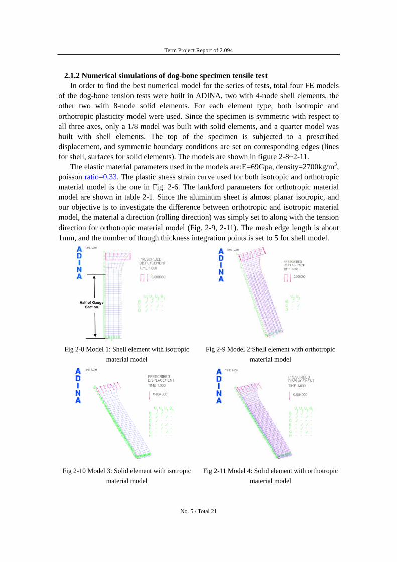
Term Project Report of 2094
212 Numerical simulations of dog-bone specimen tensile test In order to find the best numerical model for the series of tests total four FE models
of the dog-bone tension tests were built in ADINA two with 4-node shell elements the other two with 8-node solid elements For each element type both isotropic and orthotropic plasticity model were used Since the specimen is symmetric with respect to all three axes only a 18 model was built with solid elements and a quarter model was built with shell elements The top of the specimen is subjected to a prescribed displacement and symmetric boundary conditions are set on corresponding edges (lines for shell surfaces for solid elements) The models are shown in figure 2-8~2-11
The elastic material parameters used in the models areE=69Gpa density=2700kgm3 poisson ratio=033 The plastic stress strain curve used for both isotropic and orthotropic material model is the one in Fig 2-6 The lankford parameters for orthotropic material model are shown in table 2-1 Since the aluminum sheet is almost planar isotropic and our objective is to investigate the difference between orthotropic and isotropic material model the material a direction (rolling direction) was simply set to along with the tension direction for orthotropic material model (Fig 2-9 2-11) The mesh edge length is about 1mm and the number of though thickness integration points is set to 5 for shell model
Fig 2-8 Model 1 Shell element with isotropic material model
Fig 2-9 Model 2Shell element with orthotropic material model
Fig 2-10 Model 3 Solid element with isotropic material model
Fig 2-11 Model 4 Solid element with orthotropic material model
No 5 Total 21
Term Project Report of 2094
To obtain the force-displacement response a time function is defined for the prescribed displacement and the time step is 001s The analysis assumptions are large displacement and strain and a full Newton method was used for iteration All the models are run in the environment of ADINA statics hereafter in this report
Fig 2-3 shows that the average gauge section elongation to fracture is 61mm The corresponding deformation shape and effective plastic strain band plot at the fracture point are shown in Fig 2-12~2-15 The deformation figures shows that only model 3 which is with isotropic material model and solid elements can predict the necking phenomenon before fracture see Fig 216
Fig 2-12 Deformation and strain output of model 1 Fig 2-13 Deformation and strain output of model 2
Fig 2-14 Deformation and strain output of model 3 Fig 2-15 Deformation and strain output of model 4
Fig 2-16 Necking occurs in tensile tests From the simulation result the total reaction force of the top nodes and the gauge
No 6 Total 21
Term Project Report of 2094
nodes displacement can be obtained The load displacement responses and the experimental results were compared in Fig 2-17 Apparently the model 3 result accords with experimental result very well
Load
(kN
) 12
10
8
6
4
2
0
Test Result Model1Shell+Isotropy Model2Shell+Orthotropy Model3Solid+Isotropy Model4Solid+Orthotropy
00 05 10 15 20 25 30 35 40 45 50 55 60 65 70
Elongation (mm)
Fig 2-17 Comparison of load-displacement curves between experiment and simulations Previous research of ICL shows that the crack initiates at the center of the dog-bone
specimen in a tensile test Therefore the equivalent plastic strains of the central element at the fracture elongation point obtained from the numerical models were summarized in table 2-2 and compared with the fracture strain measure from thickness and width reduction of specimens (low precision) Again model 3 gives the best prediction of the local equivalent strain to fracture Hence one can conclude that the model with solid elements and isotropic plasticity model can give accurate numerical prediction for the dog-bone specimen tensile tests The reason why the shell element can not give good prediction might be that the width thickness ratio of the specimen cross-section is not big enough for a shell assumption
One can also obtain the stress triaxiality information (negative pressure divided by effective stress) of the central point of the specimen from numerical simulation The evolution of stress triaxiality with the elongation of the gauge section is shown in Fig 2-18 The average triaxiality value up to fracture is about 0345 and the triaxiality before necking is exactly equal to the analytical value 13 The average stress triaxiality would be used for fracture calibration together with the fracture strain Table 2-2 Comparison of equivalent strain to fracture of dog-bone specimen between simulations and
test of dog-bone specimens
Model 1 Model 2 Model 3 Model 4 Measurement after test
Fracture strain 012 013 048 010 053
No 7 Total 21
Term Project Report of 2094
Stre
ss T
riaxi
ality
045
044
043
042
041
040
039
038
037
036
035
034
033
032 Fracture 031
030 00 05 10 15 20 25 30 35 40 45 50 55 60 65
Elongation (mm)
Fig 2-18 Evolution of stress triaxiality calculated by ADINA
22 Flat specimen with cutouts The flat specimen with cutouts was used to obtain additional point for the calibration
of the ductile fracture model of our aluminum sheets The geometry of the specimen is shown in Fig 2-19 The initial stress triaxiality in a tensile test of this specimen can be easily controlled by changing the diameter of the cutout contour The geometry of the specimens in this project gives an analytical initial triaxiality of 052 Two FE models were set up in ADINA with 4-node shell elements and 8-node solid elements respectively With the symmetric conditions one only need to build a 14 model of the gauge section with shell elements and a 18 model of the gauge section with solid elements Fig 2-20 and Fig 2-21 shows the deformation and equivalent plastic strain contour of these two models at the fracture elongation point
Based on the studies in section 21 only isotropic material model was used for the simulations hereafter and the true stress strain curve in Fig 2-6 was adopted The mesh edge length of both models is 1mm 5 through thickness Gauss integration points were used in the shell element model The effect of the through thickness integration point number will be discussed in section 3
Fig 2-19 Geometry of flat specimen with cutouts
No 8 Total 21
Term Project Report of 2094
Fig 2-20 Deformation and strain output at fracture Fig 2-21 Deformation and strain output at fracture elongation point of shell element model elongation point of solid element model The load displacement responses and the experimental results were compared in Fig
2-22 Apparently the shell element model result correlates with experimental result better For this specimen crack also initiate at the center point of the specimen so the equivalent plastic strains to fracture of the central elements of the two models were obtained from the ADINA models and are shown in table 2-3 together with the fracture strain measured after test The shell element model gives a better prediction of equivalent strain to fracture than the solid element model
Load
(kN
)
14
12
10
8
6
4
2
0
Test Result Solid element model Shell element model
00 01 02 03 04 05 06 07 08 09 10 11 12 13
Elongation(mm)
Fig 2-22 Comparison of the load-elongation curves between FE models and test Table 2-3 Comparison of equivalent strain to fracture between simulations and test
Shell Model Solid Model Test Measurement Fracture strain 021 013 025
The evolution of stress triaxiality with the elongation of the gauge section of this specimen calculated by the shell element model is shown in Fig 2-23 The average triaxiality value up to fracture is about 051 and very close to the analytical value 052 The average stress triaxiality would be used for fracture calibration together with the fracture strain
No 9 Total 21
Term Project Report of 2094
Stre
ss T
riaxi
ality
060
055
050
045 02 04 06 08 10 12 14
Elongation(mm)
Fig 2-23 Evolution of stress triaxility of the flat specimen with cutouts
23 Flat grooved plane strain specimen Another type of specimen for the fracture calibration tests is the flat grooved
specimen which can provide a plane strain condition in the uniaxial tensile test The geometry of the specimen and a tested specimen is shown in Fig 2-24 Two FE models were set up in ADINA with 4-node plane strain elements and 8-node solid elements respectively With the symmetric conditions one only need to build a 14 model of the gauge section with plane strain elements and a 18 model of the gauge section with solid elements Fig 2-25 and Fig 2-26 show the two models
The load displacement responses and the experimental results were compared in Fig 2-27 For this specimen crack also initiate at the center point of the specimen so the equivalent plastic strains to fracture of the central elements of the two models were obtained from the ADINA models and are shown in table 2-4 together with the fracture strain measured after test using digital image correlation method
(a) Geometry of flat grooved specimen (b)A tested specimen Fig 2-24
No 10 Total 21
Term Project Report of 2094
Fig 2-25 Plane strain element model Fig 2-26 Solid element model
20 19 Test result18 Plane strain element model17
Solid element model 16 15 14 13 12 11 10 9 8 7 6 5 4 3 2 1 0000 005 010 015 020 025 030 035 040 045 050 055 060
Elongation(mm)
Load
(kN
)
Fig 2-27 Comparison of the load-elongation curves between FE models and test of plane strain specimen
Table 2-4 Comparison of equivalent strain to fracture of plane strain specimen
Plane Strain Model Solid Model Test Measurement Fracture strain 0139 0138 020
From Fig 2-27 and table 2-4 one can see that plane strain element and solid element model give almost identical prediction of load-displacement response and local strain at the center point of the specimen However using plane strain elements can greatly reduce the number of elements and thus save CPU time Fig 2-28 demonstrate that the strain in x direction is almost zero so the plane strain element is good enough to modeling tension test of this specimen
The evolution of stress triaxialities with the elongation of the gauge section of the plane strain specimen calculated by two models are shown in Fig 2-29 The average triaxiality value up to fracture is about 0572 and very close to the analytical value 0577 The average stress triaxiality would be used for fracture calibration together with the fracture strain
No 11 Total 21
Term Project Report of 2094
Fig 2-28 The band plot of the strain in XX direction
Plane strain element model
Stre
ss T
riaxi
ality
060
056
052
048
Solid element model
Fracture
01 02 03 04 05 06
Elongation(mm)
Fig 2-29 Evolution of stress triaxility of the flat grooved plane strain specimen
24 Punch indentation tests on circular disks This test provides information on fraction under the equi-biaxial state of stress
The most highly stressed point is located at the apex of the dome where the components of radial and circumferential stress and strain are equal to each other The disk specimens were secured to the 100mm diameter die by a heavy flange with 8 bolts The radius of the hemi-spherical punch was 45mm The load-displacement characteristics were recorded in the tests The measured displacement to fracture in our case was 274mm The tests were interrupted right after formation of nearly straight crack shown as shown in Fig 2-30
Accordingly a FE model of this test was built in ADINA with 4-node axisymmetric elements which is shown in Fig 2-31 The mesh edge length is 1mm The edge nodes of the disk model were fixed at all degree of freedom the center nodes of the disk model were given a symmetric boundary condition and the punch surface was given a prescribed downward displacement The contact surface on the punch was modeled as rigid and the friction coefficient is set to 001 The pressuredisplacement mixed interpolation function was used for this model to get better stress triaxiality prediction the difference between displacement-based and up mixed element will be discussed in
No 12 Total 21
Term Project Report of 2094
section 3 The time step was set to 0005s The deformation and the effective strain distribution of the disk were shown in Fig 2-32
Fig 2-30 A view of the fractured disk Fig 2-31 Numerical model of the punch test
Fig 2-32 Deformation and distribution of the disk specimen calculated by ADINA
The force displacement response can be obtained by plotting the reaction force on the punch and the displacement of the punch The comparison of the force displacement response between simulation and test result is shown in Fig 2-33 There is an excellent agreement of the measured load-displacement curve with the numerical model Also the history of the effective strain and stress triaxiality of the outer element at the apex of the dome was shown in Fig 2-34 from which one can obtain the equivalent strain to fracture of this specimen and the average stress triaxiality up to fracture of the fracture initiation point (apex of the dome) For the case of our aluminum sheet the calculated fracture strain is 063 which is very close to the strain value 069 from the measurement of thickness reduction after test The average triaxiality value up to fracture is about 065 and very close to the analytical value 23 The average stress triaxiality would be used for
No 13 Total 21
Term Project Report of 2094
fracture calibration together with the fracture strain 063
100
Forc
e(kN
)
90
80
70
60
50
40
30
20
10
0
Test result Numerical simulation
0 5 10 15 20 25 30 35
Displacement(mm)
Fig2-33 Comparison of the force displacement response of a punch test between test result and simulation output
00
02
04
06
08
10
12
14
16
18
20
Stre
ss T
riaxi
ality
Equi
vale
nt P
last
ic S
train
Equivalent plstic strain Stress triaxiality
Fracture
0 2 4 6 8 10 12 14 16 18 20 22 24 26 28 30 32 34 36 38 40
Displacement (mm)
Fig 2-34 Evolution of equivalent plastic strain and stress triaxiality at the fracture initiation point
25 Ductile fracture calibration using simulation results As all the numerical simulations of calibration tests has been performed and validated
by experimental results a fracture locus of our aluminum sheets can be calibrated with the simulation results Table 2-5 shows all the fracture points obtained from the numerical simulation
Table 2-5 Fracture points obtained from numerical simulations Point Specimen Type Stress Triaxiality Fracture Strain
1 Dog-bone 0345 048 2 Flat with cutouts 051 021 3 Flat grooved 0572 014 4 Punch indentation 065 063
No 14 Total 21
Term Project Report of 2094
A Mohr-Coulomb fracture criterion was used to calibrate the fracture locus of this aluminum sheet The form of this fracture criterion in the space of fracture strain and stress triaxiality is as followed
minus1
ε f = ⎨⎪⎧
⎪⎩cA 2
f3 ⎢⎡
⎣⎢⎜⎛
⎝⎜
1+ 3 c1
2
sdot f1 ⎟⎞⎟⎠+ c1
⎛⎜⎝η +
f 3
2 ⎞⎟⎠⎥⎤
⎥⎦
⎪⎬⎫
⎭⎪
n
(2-3)
where the functions f1 f2 and f3 are defined as
f1 1 27 η η 2 = cos arcsin ⎢
⎡minus ( minus 1)⎤⎥3 ⎣ 2 3 ⎦
( 2f2 = sin 1 arcsin ⎡minus 27 η η minus 1)⎤ (2-4) 3 ⎣⎢ 2 3 ⎥⎦
f3 c3 3 (1minus c3)( 1 minus1)= +
2 minus 3 f1
This fracture criterion is a function of equivalent strain to fracture ε f in terms of the
average stress triaxiality η up to fracture A and n are the material parameters in Eq
(2-1) This criterion has 3 calibration parameters c1c2 and c3 Hence points 1 3 and 4 in table 2-5 were used to calibrate the 3 free parameters while point 2 was used to validate the accuracy of the fracture locus The calibrated fracture locus is shown in Fig 2-35 One can see that the calibrated fracture locus can predict the fracture strain at point 2 (flat specimen with side cutouts) with good accuracy Therefore this fracture locus can be implemented into the FE codes to predict ductile fracture during calculations
c1=0154 c2=248MPa c3=098 A=438MPa n=007
Calibration Points
Validation Point
Fig2-35 Calibrated fracture locus of our aluminum sheets with numerical results
No 15 Total 21
Term Project Report of 2094
3 Parametric Study of Some Numerical Simulation Parameters To predict the initial crack position accurately the local strain and stress triaxiality are
very important to the fracture identification However some parameters may affect the local strainstress significantly such as number of integration points (NIP) through thickness element type mesh size and so on
Several finite element models were built based on the benchmark models in section 2 to study these effects The force-displacement response effective strain and stress triaxilality history at the initial crack position were compared and analyzed
31 Effect of Number of Integration Point through thickness (NIP) This study is based on the shell element model of the flat specimen with cutouts The
benchmark model in section 22 is with 5 integration points though thickness and the Gauss integration was used Two more shell element models of the flat specimen with cutouts with 2 and 3 through thickness integration points respectively were built in ADINA
As is shown in Fig 3-1 as the NIP through thickness of shell elements increases the load-elongation response predicted by the numerical model is closer to the experimental results From Fig 3-2 and 3-3 one can see that the local strain and stress triaxiality at the crack initiation point (the center of the specimen) predicted by the 2 NIP model are much lower than the 5 NIP model which has shown good accuracy in section 22 Hence if shell elements are used for numerical simulations of similar problems at least 5 through thickness integration points should be employed
Load
(kN
)
17 16 15 14 13 12 11 10 9 8 7 6 5 4 3 2 1 0
Test INP=2 INP=3 INP=5
Fracture
00 01 02 03 04 05 06 07 08 09 10 11 12 13 14 15
Elongation(mm)
Fig 3-1 Load-elongation responses of three models with different NIP through thickness
No 16 Total 21
Term Project Report of 2094
Equ
ival
ent P
last
ic S
train
10
09
08
07
06
05
04
03
02
01
00
INP=2 INP=3 INP=5
Fracture
00 02 04 06 08 10 12 14 16 18 20
Elongation(mm)
Fig 3-2 Strain history at crack initiation point of three models with different NIP through thickness
044
046
048
050
052
054
056
058
Stre
ss T
riaxi
ality
NIP=2 NIP=3 NIP=5
Fracture
02 04 06 08 10 12 14
Elongation(mm)
Fig 3-3 Stress triaxiality history at crack initiation point of three models with different NIP through thickness
32 Effect of element type This study is based on the model of punch indentation tests in section 24 Three
different models with different element types and interpolation formulations were
No 17 Total 21
Term Project Report of 2094
compared in this section displacement based 4-node element mixed 41 and 93 up element
From Fig3-4 and Fig 3-5 one can see that the force-displacement response and local strain evolution at the crack initiation point (the apex of the dome) are not affected much by the element type However as is shown in Fig 3-6 the displacement based element can not predict the stress triaxiality well because the analytical stress triaxiality value should be 23 in this test Since stress triaxiality is a normalized pressure the low accuracy triaxiality prediction is due to the unreasonable pressure distribution and magnitudes predicted by the displacement-based elements as is shown in Fig 3-7 The pressure distribution calculated by mixed up elements are much more accurate as is shown in Fig 3-8
Test 4-node displacement based element 41 mixed up element 93 mixed up element
Fracture
0 5 10 15 20 25 30 35 40 45 50
Displacement(mm)
Equ
ival
ent P
last
ic S
train
07
06
05
04
03
02
01
0 2 4 6 8 10 12 14 16 18 20 22 24 26 28
4-node displacement based element 41 mixed up element 93 mixed up element
Fracture
120
110
100
90
80
Forc
e(kN
)
70
60
50
40
30
20
10
0 00
Displacement(mm)
Fig 3-4 Force-displacement responses of 3 models Fig 3-5 Equivalent plastic strain evolution at crack with different element types initiation point of 3 models with different element
types
10
05
00
4-node displacment based elment 41 mixed up element 93 mixed up element
-05
-10
-15
-20
-25
-30
-35
-40
-45
-50
Stre
ss T
riaxi
ality
0 5 10 15 20 25 30
Displacement(mm)
Fig 3-6 Evolution of stress triaxiality at crack initiation point of 3 element types
No 18 Total 21
Term Project Report of 2094
Fig 3-7 Pressure distribution of the model with 4 node Fig 3-8 Pressure distribution of the model with 93 displacement based elments mixed elements
33 Mesh size effect This study is based on the model of punch indentation tests in section 24 Three
different models with different mesh sizes were built as is shown in Fig 3-9 and the force-displacement responses local strain and stress triaxiality history at the crach initiation point (the apex of the dome) were compared and studied The 3 different mesh edge length studied in this section was 1mm 05mm and 2mm The 41 mixed up elements were employed in all three models
Fig 3-10 and 3-11 show that the force-displacement response and stress triaxiality predicted by the numerical models become closer to the experimental result or analytical result as the mesh goes finer As is shown by Fig 3-12 the local strain seems to be larger as the mesh edge length is smaller in the early stage but it reach convergence finally Hence the finite element model is convergent as the mesh becomes finer
(a)Mesh edge length=1mm (b)Mesh edge length=05mm (c)Mesh edge length=2mm Fig 3-9 Three models with different mesh size
No 19 Total 21
Term Project Report of 2094
Test Mesh edge length=1mm 08
Mesh edge length=1mm Mesh edge length=2mm Mesh edge length=05mm
Mesh edge length=05mm Mesh edge length=2mm
120
110
100
07
06 90
80
Stre
ss T
riaxi
ality
05
04
03 Forc
e(kN
)
70
60
50
40
30
20
02
01
00
10
0 0 5 10 15 20 25 30 35 40 45 50 0 5 10 15 20 25 30 35 40 45 50
Displacement(mm) Displacement(mm)
Fig 3-10 Force-displacement responses of 3 models Fig 3-11 Evolution of stress triaxiality at crack with different element size initiation point of 3 models with different element size
10
Mesh edge length=1mm 08 Mesh edge length=05mm Mesh edge length=2mm
Equi
vale
nt P
lstic
Stra
in
06
04
02
00 0 5 10 15 20 25 30
Displacement(mm)
Fig 3-12 Equivalent plastic strain evolution at crack initiation point of 3 models with different element size
No 20 Total 21
Term Project Report of 2094
4 Conclusions In this project four types of specimens made from our aluminum sheets were tested
in the lab to investigate the fracture characteristics of this material At the same time corresponding finite element models were built to simulate the fracture calibration tests Most suited model for each test was determined after comparisons and analysis and the fracture locus of this material was calibrated with the simulation results Moreover a brief parametric study was performed to evaluate the effect of several FE parameters on the numerical simulation results Main conclusions are shown as followed
1) Finite element model can simulate the physical problems very well Suited FE models can predict the load-displacement responses local strain and stress with good accuracy
2) Selection of element type and modeling strategy should depend on the geometry and boundary conditions of the physical problem For this project one should choose solid elements for dog-bone specimen shell elements for flat specimen with cutouts plane strain elements for flat grooved specimen and axisymmetric elements for the punch indentation test
3) Number of integration points (NIP) through thickness has a great effect on the strain and stress distribution of shell elements Once the through thickness stress gradient is involved in a physical problem such as necking or bending a larger NIP through thickness should be employed
4) The up mixed element can predict the pressure distribution and magnitude much more accurate
5) The FE models in this project are convergent As the mesh becomes finer both the load-displacement response and local stressstrain output become closer to experimental results or analytical values
No 21 Total 21
MIT OpenCourseWare httpocwmitedu
2094 Finite Element Analysis of Solids and Fluids IISpring 2011
For information about citing these materials or our Terms of Use visit httpocwmiteduterms
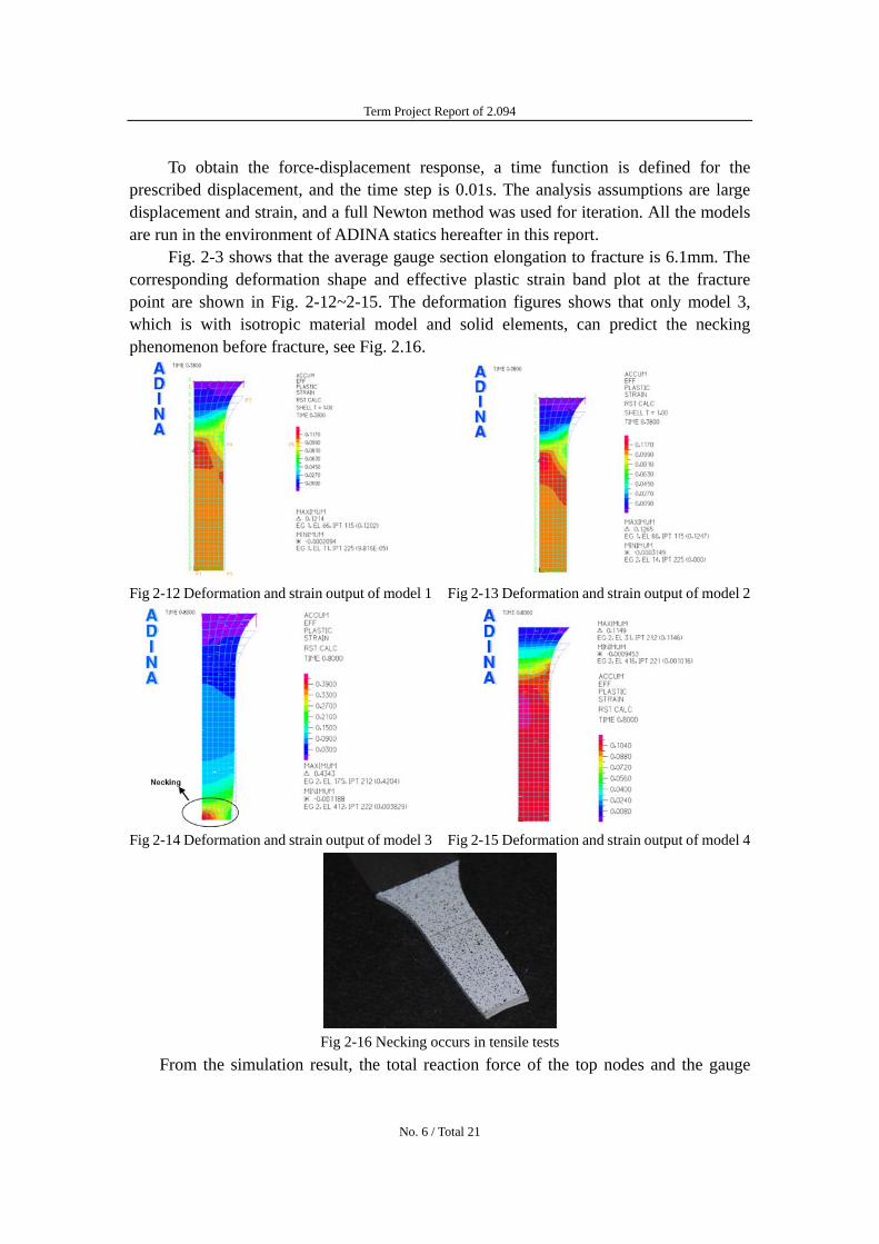
Term Project Report of 2094
nodes displacement can be obtained The load displacement responses and the experimental results were compared in Fig 2-17 Apparently the model 3 result accords with experimental result very well
Load
(kN
) 12
10
8
6
4
2
0
Test Result Model1Shell+Isotropy Model2Shell+Orthotropy Model3Solid+Isotropy Model4Solid+Orthotropy
00 05 10 15 20 25 30 35 40 45 50 55 60 65 70
Elongation (mm)
Fig 2-17 Comparison of load-displacement curves between experiment and simulations Previous research of ICL shows that the crack initiates at the center of the dog-bone
specimen in a tensile test Therefore the equivalent plastic strains of the central element at the fracture elongation point obtained from the numerical models were summarized in table 2-2 and compared with the fracture strain measure from thickness and width reduction of specimens (low precision) Again model 3 gives the best prediction of the local equivalent strain to fracture Hence one can conclude that the model with solid elements and isotropic plasticity model can give accurate numerical prediction for the dog-bone specimen tensile tests The reason why the shell element can not give good prediction might be that the width thickness ratio of the specimen cross-section is not big enough for a shell assumption
One can also obtain the stress triaxiality information (negative pressure divided by effective stress) of the central point of the specimen from numerical simulation The evolution of stress triaxiality with the elongation of the gauge section is shown in Fig 2-18 The average triaxiality value up to fracture is about 0345 and the triaxiality before necking is exactly equal to the analytical value 13 The average stress triaxiality would be used for fracture calibration together with the fracture strain Table 2-2 Comparison of equivalent strain to fracture of dog-bone specimen between simulations and
test of dog-bone specimens
Model 1 Model 2 Model 3 Model 4 Measurement after test
Fracture strain 012 013 048 010 053
No 7 Total 21
Term Project Report of 2094
Stre
ss T
riaxi
ality
045
044
043
042
041
040
039
038
037
036
035
034
033
032 Fracture 031
030 00 05 10 15 20 25 30 35 40 45 50 55 60 65
Elongation (mm)
Fig 2-18 Evolution of stress triaxiality calculated by ADINA
22 Flat specimen with cutouts The flat specimen with cutouts was used to obtain additional point for the calibration
of the ductile fracture model of our aluminum sheets The geometry of the specimen is shown in Fig 2-19 The initial stress triaxiality in a tensile test of this specimen can be easily controlled by changing the diameter of the cutout contour The geometry of the specimens in this project gives an analytical initial triaxiality of 052 Two FE models were set up in ADINA with 4-node shell elements and 8-node solid elements respectively With the symmetric conditions one only need to build a 14 model of the gauge section with shell elements and a 18 model of the gauge section with solid elements Fig 2-20 and Fig 2-21 shows the deformation and equivalent plastic strain contour of these two models at the fracture elongation point
Based on the studies in section 21 only isotropic material model was used for the simulations hereafter and the true stress strain curve in Fig 2-6 was adopted The mesh edge length of both models is 1mm 5 through thickness Gauss integration points were used in the shell element model The effect of the through thickness integration point number will be discussed in section 3
Fig 2-19 Geometry of flat specimen with cutouts
No 8 Total 21
Term Project Report of 2094
Fig 2-20 Deformation and strain output at fracture Fig 2-21 Deformation and strain output at fracture elongation point of shell element model elongation point of solid element model The load displacement responses and the experimental results were compared in Fig
2-22 Apparently the shell element model result correlates with experimental result better For this specimen crack also initiate at the center point of the specimen so the equivalent plastic strains to fracture of the central elements of the two models were obtained from the ADINA models and are shown in table 2-3 together with the fracture strain measured after test The shell element model gives a better prediction of equivalent strain to fracture than the solid element model
Load
(kN
)
14
12
10
8
6
4
2
0
Test Result Solid element model Shell element model
00 01 02 03 04 05 06 07 08 09 10 11 12 13
Elongation(mm)
Fig 2-22 Comparison of the load-elongation curves between FE models and test Table 2-3 Comparison of equivalent strain to fracture between simulations and test
Shell Model Solid Model Test Measurement Fracture strain 021 013 025
The evolution of stress triaxiality with the elongation of the gauge section of this specimen calculated by the shell element model is shown in Fig 2-23 The average triaxiality value up to fracture is about 051 and very close to the analytical value 052 The average stress triaxiality would be used for fracture calibration together with the fracture strain
No 9 Total 21
Term Project Report of 2094
Stre
ss T
riaxi
ality
060
055
050
045 02 04 06 08 10 12 14
Elongation(mm)
Fig 2-23 Evolution of stress triaxility of the flat specimen with cutouts
23 Flat grooved plane strain specimen Another type of specimen for the fracture calibration tests is the flat grooved
specimen which can provide a plane strain condition in the uniaxial tensile test The geometry of the specimen and a tested specimen is shown in Fig 2-24 Two FE models were set up in ADINA with 4-node plane strain elements and 8-node solid elements respectively With the symmetric conditions one only need to build a 14 model of the gauge section with plane strain elements and a 18 model of the gauge section with solid elements Fig 2-25 and Fig 2-26 show the two models
The load displacement responses and the experimental results were compared in Fig 2-27 For this specimen crack also initiate at the center point of the specimen so the equivalent plastic strains to fracture of the central elements of the two models were obtained from the ADINA models and are shown in table 2-4 together with the fracture strain measured after test using digital image correlation method
(a) Geometry of flat grooved specimen (b)A tested specimen Fig 2-24
No 10 Total 21
Term Project Report of 2094
Fig 2-25 Plane strain element model Fig 2-26 Solid element model
20 19 Test result18 Plane strain element model17
Solid element model 16 15 14 13 12 11 10 9 8 7 6 5 4 3 2 1 0000 005 010 015 020 025 030 035 040 045 050 055 060
Elongation(mm)
Load
(kN
)
Fig 2-27 Comparison of the load-elongation curves between FE models and test of plane strain specimen
Table 2-4 Comparison of equivalent strain to fracture of plane strain specimen
Plane Strain Model Solid Model Test Measurement Fracture strain 0139 0138 020
From Fig 2-27 and table 2-4 one can see that plane strain element and solid element model give almost identical prediction of load-displacement response and local strain at the center point of the specimen However using plane strain elements can greatly reduce the number of elements and thus save CPU time Fig 2-28 demonstrate that the strain in x direction is almost zero so the plane strain element is good enough to modeling tension test of this specimen
The evolution of stress triaxialities with the elongation of the gauge section of the plane strain specimen calculated by two models are shown in Fig 2-29 The average triaxiality value up to fracture is about 0572 and very close to the analytical value 0577 The average stress triaxiality would be used for fracture calibration together with the fracture strain
No 11 Total 21
Term Project Report of 2094
Fig 2-28 The band plot of the strain in XX direction
Plane strain element model
Stre
ss T
riaxi
ality
060
056
052
048
Solid element model
Fracture
01 02 03 04 05 06
Elongation(mm)
Fig 2-29 Evolution of stress triaxility of the flat grooved plane strain specimen
24 Punch indentation tests on circular disks This test provides information on fraction under the equi-biaxial state of stress
The most highly stressed point is located at the apex of the dome where the components of radial and circumferential stress and strain are equal to each other The disk specimens were secured to the 100mm diameter die by a heavy flange with 8 bolts The radius of the hemi-spherical punch was 45mm The load-displacement characteristics were recorded in the tests The measured displacement to fracture in our case was 274mm The tests were interrupted right after formation of nearly straight crack shown as shown in Fig 2-30
Accordingly a FE model of this test was built in ADINA with 4-node axisymmetric elements which is shown in Fig 2-31 The mesh edge length is 1mm The edge nodes of the disk model were fixed at all degree of freedom the center nodes of the disk model were given a symmetric boundary condition and the punch surface was given a prescribed downward displacement The contact surface on the punch was modeled as rigid and the friction coefficient is set to 001 The pressuredisplacement mixed interpolation function was used for this model to get better stress triaxiality prediction the difference between displacement-based and up mixed element will be discussed in
No 12 Total 21
Term Project Report of 2094
section 3 The time step was set to 0005s The deformation and the effective strain distribution of the disk were shown in Fig 2-32
Fig 2-30 A view of the fractured disk Fig 2-31 Numerical model of the punch test
Fig 2-32 Deformation and distribution of the disk specimen calculated by ADINA
The force displacement response can be obtained by plotting the reaction force on the punch and the displacement of the punch The comparison of the force displacement response between simulation and test result is shown in Fig 2-33 There is an excellent agreement of the measured load-displacement curve with the numerical model Also the history of the effective strain and stress triaxiality of the outer element at the apex of the dome was shown in Fig 2-34 from which one can obtain the equivalent strain to fracture of this specimen and the average stress triaxiality up to fracture of the fracture initiation point (apex of the dome) For the case of our aluminum sheet the calculated fracture strain is 063 which is very close to the strain value 069 from the measurement of thickness reduction after test The average triaxiality value up to fracture is about 065 and very close to the analytical value 23 The average stress triaxiality would be used for
No 13 Total 21
Term Project Report of 2094
fracture calibration together with the fracture strain 063
100
Forc
e(kN
)
90
80
70
60
50
40
30
20
10
0
Test result Numerical simulation
0 5 10 15 20 25 30 35
Displacement(mm)
Fig2-33 Comparison of the force displacement response of a punch test between test result and simulation output
00
02
04
06
08
10
12
14
16
18
20
Stre
ss T
riaxi
ality
Equi
vale
nt P
last
ic S
train
Equivalent plstic strain Stress triaxiality
Fracture
0 2 4 6 8 10 12 14 16 18 20 22 24 26 28 30 32 34 36 38 40
Displacement (mm)
Fig 2-34 Evolution of equivalent plastic strain and stress triaxiality at the fracture initiation point
25 Ductile fracture calibration using simulation results As all the numerical simulations of calibration tests has been performed and validated
by experimental results a fracture locus of our aluminum sheets can be calibrated with the simulation results Table 2-5 shows all the fracture points obtained from the numerical simulation
Table 2-5 Fracture points obtained from numerical simulations Point Specimen Type Stress Triaxiality Fracture Strain
1 Dog-bone 0345 048 2 Flat with cutouts 051 021 3 Flat grooved 0572 014 4 Punch indentation 065 063
No 14 Total 21
Term Project Report of 2094
A Mohr-Coulomb fracture criterion was used to calibrate the fracture locus of this aluminum sheet The form of this fracture criterion in the space of fracture strain and stress triaxiality is as followed
minus1
ε f = ⎨⎪⎧
⎪⎩cA 2
f3 ⎢⎡
⎣⎢⎜⎛
⎝⎜
1+ 3 c1
2
sdot f1 ⎟⎞⎟⎠+ c1
⎛⎜⎝η +
f 3
2 ⎞⎟⎠⎥⎤
⎥⎦
⎪⎬⎫
⎭⎪
n
(2-3)
where the functions f1 f2 and f3 are defined as
f1 1 27 η η 2 = cos arcsin ⎢
⎡minus ( minus 1)⎤⎥3 ⎣ 2 3 ⎦
( 2f2 = sin 1 arcsin ⎡minus 27 η η minus 1)⎤ (2-4) 3 ⎣⎢ 2 3 ⎥⎦
f3 c3 3 (1minus c3)( 1 minus1)= +
2 minus 3 f1
This fracture criterion is a function of equivalent strain to fracture ε f in terms of the
average stress triaxiality η up to fracture A and n are the material parameters in Eq
(2-1) This criterion has 3 calibration parameters c1c2 and c3 Hence points 1 3 and 4 in table 2-5 were used to calibrate the 3 free parameters while point 2 was used to validate the accuracy of the fracture locus The calibrated fracture locus is shown in Fig 2-35 One can see that the calibrated fracture locus can predict the fracture strain at point 2 (flat specimen with side cutouts) with good accuracy Therefore this fracture locus can be implemented into the FE codes to predict ductile fracture during calculations
c1=0154 c2=248MPa c3=098 A=438MPa n=007
Calibration Points
Validation Point
Fig2-35 Calibrated fracture locus of our aluminum sheets with numerical results
No 15 Total 21
Term Project Report of 2094
3 Parametric Study of Some Numerical Simulation Parameters To predict the initial crack position accurately the local strain and stress triaxiality are
very important to the fracture identification However some parameters may affect the local strainstress significantly such as number of integration points (NIP) through thickness element type mesh size and so on
Several finite element models were built based on the benchmark models in section 2 to study these effects The force-displacement response effective strain and stress triaxilality history at the initial crack position were compared and analyzed
31 Effect of Number of Integration Point through thickness (NIP) This study is based on the shell element model of the flat specimen with cutouts The
benchmark model in section 22 is with 5 integration points though thickness and the Gauss integration was used Two more shell element models of the flat specimen with cutouts with 2 and 3 through thickness integration points respectively were built in ADINA
As is shown in Fig 3-1 as the NIP through thickness of shell elements increases the load-elongation response predicted by the numerical model is closer to the experimental results From Fig 3-2 and 3-3 one can see that the local strain and stress triaxiality at the crack initiation point (the center of the specimen) predicted by the 2 NIP model are much lower than the 5 NIP model which has shown good accuracy in section 22 Hence if shell elements are used for numerical simulations of similar problems at least 5 through thickness integration points should be employed
Load
(kN
)
17 16 15 14 13 12 11 10 9 8 7 6 5 4 3 2 1 0
Test INP=2 INP=3 INP=5
Fracture
00 01 02 03 04 05 06 07 08 09 10 11 12 13 14 15
Elongation(mm)
Fig 3-1 Load-elongation responses of three models with different NIP through thickness
No 16 Total 21
Term Project Report of 2094
Equ
ival
ent P
last
ic S
train
10
09
08
07
06
05
04
03
02
01
00
INP=2 INP=3 INP=5
Fracture
00 02 04 06 08 10 12 14 16 18 20
Elongation(mm)
Fig 3-2 Strain history at crack initiation point of three models with different NIP through thickness
044
046
048
050
052
054
056
058
Stre
ss T
riaxi
ality
NIP=2 NIP=3 NIP=5
Fracture
02 04 06 08 10 12 14
Elongation(mm)
Fig 3-3 Stress triaxiality history at crack initiation point of three models with different NIP through thickness
32 Effect of element type This study is based on the model of punch indentation tests in section 24 Three
different models with different element types and interpolation formulations were
No 17 Total 21
Term Project Report of 2094
compared in this section displacement based 4-node element mixed 41 and 93 up element
From Fig3-4 and Fig 3-5 one can see that the force-displacement response and local strain evolution at the crack initiation point (the apex of the dome) are not affected much by the element type However as is shown in Fig 3-6 the displacement based element can not predict the stress triaxiality well because the analytical stress triaxiality value should be 23 in this test Since stress triaxiality is a normalized pressure the low accuracy triaxiality prediction is due to the unreasonable pressure distribution and magnitudes predicted by the displacement-based elements as is shown in Fig 3-7 The pressure distribution calculated by mixed up elements are much more accurate as is shown in Fig 3-8
Test 4-node displacement based element 41 mixed up element 93 mixed up element
Fracture
0 5 10 15 20 25 30 35 40 45 50
Displacement(mm)
Equ
ival
ent P
last
ic S
train
07
06
05
04
03
02
01
0 2 4 6 8 10 12 14 16 18 20 22 24 26 28
4-node displacement based element 41 mixed up element 93 mixed up element
Fracture
120
110
100
90
80
Forc
e(kN
)
70
60
50
40
30
20
10
0 00
Displacement(mm)
Fig 3-4 Force-displacement responses of 3 models Fig 3-5 Equivalent plastic strain evolution at crack with different element types initiation point of 3 models with different element
types
10
05
00
4-node displacment based elment 41 mixed up element 93 mixed up element
-05
-10
-15
-20
-25
-30
-35
-40
-45
-50
Stre
ss T
riaxi
ality
0 5 10 15 20 25 30
Displacement(mm)
Fig 3-6 Evolution of stress triaxiality at crack initiation point of 3 element types
No 18 Total 21
Term Project Report of 2094
Fig 3-7 Pressure distribution of the model with 4 node Fig 3-8 Pressure distribution of the model with 93 displacement based elments mixed elements
33 Mesh size effect This study is based on the model of punch indentation tests in section 24 Three
different models with different mesh sizes were built as is shown in Fig 3-9 and the force-displacement responses local strain and stress triaxiality history at the crach initiation point (the apex of the dome) were compared and studied The 3 different mesh edge length studied in this section was 1mm 05mm and 2mm The 41 mixed up elements were employed in all three models
Fig 3-10 and 3-11 show that the force-displacement response and stress triaxiality predicted by the numerical models become closer to the experimental result or analytical result as the mesh goes finer As is shown by Fig 3-12 the local strain seems to be larger as the mesh edge length is smaller in the early stage but it reach convergence finally Hence the finite element model is convergent as the mesh becomes finer
(a)Mesh edge length=1mm (b)Mesh edge length=05mm (c)Mesh edge length=2mm Fig 3-9 Three models with different mesh size
No 19 Total 21
Term Project Report of 2094
Test Mesh edge length=1mm 08
Mesh edge length=1mm Mesh edge length=2mm Mesh edge length=05mm
Mesh edge length=05mm Mesh edge length=2mm
120
110
100
07
06 90
80
Stre
ss T
riaxi
ality
05
04
03 Forc
e(kN
)
70
60
50
40
30
20
02
01
00
10
0 0 5 10 15 20 25 30 35 40 45 50 0 5 10 15 20 25 30 35 40 45 50
Displacement(mm) Displacement(mm)
Fig 3-10 Force-displacement responses of 3 models Fig 3-11 Evolution of stress triaxiality at crack with different element size initiation point of 3 models with different element size
10
Mesh edge length=1mm 08 Mesh edge length=05mm Mesh edge length=2mm
Equi
vale
nt P
lstic
Stra
in
06
04
02
00 0 5 10 15 20 25 30
Displacement(mm)
Fig 3-12 Equivalent plastic strain evolution at crack initiation point of 3 models with different element size
No 20 Total 21
Term Project Report of 2094
4 Conclusions In this project four types of specimens made from our aluminum sheets were tested
in the lab to investigate the fracture characteristics of this material At the same time corresponding finite element models were built to simulate the fracture calibration tests Most suited model for each test was determined after comparisons and analysis and the fracture locus of this material was calibrated with the simulation results Moreover a brief parametric study was performed to evaluate the effect of several FE parameters on the numerical simulation results Main conclusions are shown as followed
1) Finite element model can simulate the physical problems very well Suited FE models can predict the load-displacement responses local strain and stress with good accuracy
2) Selection of element type and modeling strategy should depend on the geometry and boundary conditions of the physical problem For this project one should choose solid elements for dog-bone specimen shell elements for flat specimen with cutouts plane strain elements for flat grooved specimen and axisymmetric elements for the punch indentation test
3) Number of integration points (NIP) through thickness has a great effect on the strain and stress distribution of shell elements Once the through thickness stress gradient is involved in a physical problem such as necking or bending a larger NIP through thickness should be employed
4) The up mixed element can predict the pressure distribution and magnitude much more accurate
5) The FE models in this project are convergent As the mesh becomes finer both the load-displacement response and local stressstrain output become closer to experimental results or analytical values
No 21 Total 21
MIT OpenCourseWare httpocwmitedu
2094 Finite Element Analysis of Solids and Fluids IISpring 2011
For information about citing these materials or our Terms of Use visit httpocwmiteduterms
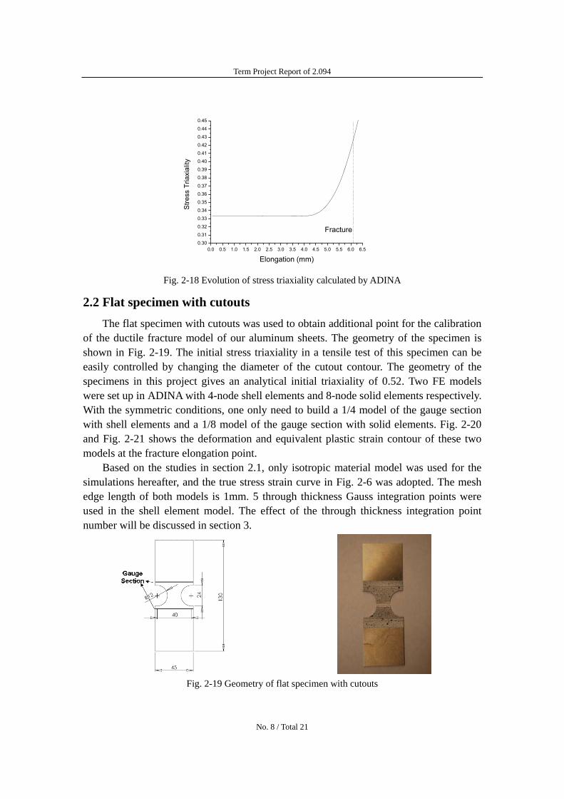
Term Project Report of 2094
Stre
ss T
riaxi
ality
045
044
043
042
041
040
039
038
037
036
035
034
033
032 Fracture 031
030 00 05 10 15 20 25 30 35 40 45 50 55 60 65
Elongation (mm)
Fig 2-18 Evolution of stress triaxiality calculated by ADINA
22 Flat specimen with cutouts The flat specimen with cutouts was used to obtain additional point for the calibration
of the ductile fracture model of our aluminum sheets The geometry of the specimen is shown in Fig 2-19 The initial stress triaxiality in a tensile test of this specimen can be easily controlled by changing the diameter of the cutout contour The geometry of the specimens in this project gives an analytical initial triaxiality of 052 Two FE models were set up in ADINA with 4-node shell elements and 8-node solid elements respectively With the symmetric conditions one only need to build a 14 model of the gauge section with shell elements and a 18 model of the gauge section with solid elements Fig 2-20 and Fig 2-21 shows the deformation and equivalent plastic strain contour of these two models at the fracture elongation point
Based on the studies in section 21 only isotropic material model was used for the simulations hereafter and the true stress strain curve in Fig 2-6 was adopted The mesh edge length of both models is 1mm 5 through thickness Gauss integration points were used in the shell element model The effect of the through thickness integration point number will be discussed in section 3
Fig 2-19 Geometry of flat specimen with cutouts
No 8 Total 21
Term Project Report of 2094
Fig 2-20 Deformation and strain output at fracture Fig 2-21 Deformation and strain output at fracture elongation point of shell element model elongation point of solid element model The load displacement responses and the experimental results were compared in Fig
2-22 Apparently the shell element model result correlates with experimental result better For this specimen crack also initiate at the center point of the specimen so the equivalent plastic strains to fracture of the central elements of the two models were obtained from the ADINA models and are shown in table 2-3 together with the fracture strain measured after test The shell element model gives a better prediction of equivalent strain to fracture than the solid element model
Load
(kN
)
14
12
10
8
6
4
2
0
Test Result Solid element model Shell element model
00 01 02 03 04 05 06 07 08 09 10 11 12 13
Elongation(mm)
Fig 2-22 Comparison of the load-elongation curves between FE models and test Table 2-3 Comparison of equivalent strain to fracture between simulations and test
Shell Model Solid Model Test Measurement Fracture strain 021 013 025
The evolution of stress triaxiality with the elongation of the gauge section of this specimen calculated by the shell element model is shown in Fig 2-23 The average triaxiality value up to fracture is about 051 and very close to the analytical value 052 The average stress triaxiality would be used for fracture calibration together with the fracture strain
No 9 Total 21
Term Project Report of 2094
Stre
ss T
riaxi
ality
060
055
050
045 02 04 06 08 10 12 14
Elongation(mm)
Fig 2-23 Evolution of stress triaxility of the flat specimen with cutouts
23 Flat grooved plane strain specimen Another type of specimen for the fracture calibration tests is the flat grooved
specimen which can provide a plane strain condition in the uniaxial tensile test The geometry of the specimen and a tested specimen is shown in Fig 2-24 Two FE models were set up in ADINA with 4-node plane strain elements and 8-node solid elements respectively With the symmetric conditions one only need to build a 14 model of the gauge section with plane strain elements and a 18 model of the gauge section with solid elements Fig 2-25 and Fig 2-26 show the two models
The load displacement responses and the experimental results were compared in Fig 2-27 For this specimen crack also initiate at the center point of the specimen so the equivalent plastic strains to fracture of the central elements of the two models were obtained from the ADINA models and are shown in table 2-4 together with the fracture strain measured after test using digital image correlation method
(a) Geometry of flat grooved specimen (b)A tested specimen Fig 2-24
No 10 Total 21
Term Project Report of 2094
Fig 2-25 Plane strain element model Fig 2-26 Solid element model
20 19 Test result18 Plane strain element model17
Solid element model 16 15 14 13 12 11 10 9 8 7 6 5 4 3 2 1 0000 005 010 015 020 025 030 035 040 045 050 055 060
Elongation(mm)
Load
(kN
)
Fig 2-27 Comparison of the load-elongation curves between FE models and test of plane strain specimen
Table 2-4 Comparison of equivalent strain to fracture of plane strain specimen
Plane Strain Model Solid Model Test Measurement Fracture strain 0139 0138 020
From Fig 2-27 and table 2-4 one can see that plane strain element and solid element model give almost identical prediction of load-displacement response and local strain at the center point of the specimen However using plane strain elements can greatly reduce the number of elements and thus save CPU time Fig 2-28 demonstrate that the strain in x direction is almost zero so the plane strain element is good enough to modeling tension test of this specimen
The evolution of stress triaxialities with the elongation of the gauge section of the plane strain specimen calculated by two models are shown in Fig 2-29 The average triaxiality value up to fracture is about 0572 and very close to the analytical value 0577 The average stress triaxiality would be used for fracture calibration together with the fracture strain
No 11 Total 21
Term Project Report of 2094
Fig 2-28 The band plot of the strain in XX direction
Plane strain element model
Stre
ss T
riaxi
ality
060
056
052
048
Solid element model
Fracture
01 02 03 04 05 06
Elongation(mm)
Fig 2-29 Evolution of stress triaxility of the flat grooved plane strain specimen
24 Punch indentation tests on circular disks This test provides information on fraction under the equi-biaxial state of stress
The most highly stressed point is located at the apex of the dome where the components of radial and circumferential stress and strain are equal to each other The disk specimens were secured to the 100mm diameter die by a heavy flange with 8 bolts The radius of the hemi-spherical punch was 45mm The load-displacement characteristics were recorded in the tests The measured displacement to fracture in our case was 274mm The tests were interrupted right after formation of nearly straight crack shown as shown in Fig 2-30
Accordingly a FE model of this test was built in ADINA with 4-node axisymmetric elements which is shown in Fig 2-31 The mesh edge length is 1mm The edge nodes of the disk model were fixed at all degree of freedom the center nodes of the disk model were given a symmetric boundary condition and the punch surface was given a prescribed downward displacement The contact surface on the punch was modeled as rigid and the friction coefficient is set to 001 The pressuredisplacement mixed interpolation function was used for this model to get better stress triaxiality prediction the difference between displacement-based and up mixed element will be discussed in
No 12 Total 21
Term Project Report of 2094
section 3 The time step was set to 0005s The deformation and the effective strain distribution of the disk were shown in Fig 2-32
Fig 2-30 A view of the fractured disk Fig 2-31 Numerical model of the punch test
Fig 2-32 Deformation and distribution of the disk specimen calculated by ADINA
The force displacement response can be obtained by plotting the reaction force on the punch and the displacement of the punch The comparison of the force displacement response between simulation and test result is shown in Fig 2-33 There is an excellent agreement of the measured load-displacement curve with the numerical model Also the history of the effective strain and stress triaxiality of the outer element at the apex of the dome was shown in Fig 2-34 from which one can obtain the equivalent strain to fracture of this specimen and the average stress triaxiality up to fracture of the fracture initiation point (apex of the dome) For the case of our aluminum sheet the calculated fracture strain is 063 which is very close to the strain value 069 from the measurement of thickness reduction after test The average triaxiality value up to fracture is about 065 and very close to the analytical value 23 The average stress triaxiality would be used for
No 13 Total 21
Term Project Report of 2094
fracture calibration together with the fracture strain 063
100
Forc
e(kN
)
90
80
70
60
50
40
30
20
10
0
Test result Numerical simulation
0 5 10 15 20 25 30 35
Displacement(mm)
Fig2-33 Comparison of the force displacement response of a punch test between test result and simulation output
00
02
04
06
08
10
12
14
16
18
20
Stre
ss T
riaxi
ality
Equi
vale
nt P
last
ic S
train
Equivalent plstic strain Stress triaxiality
Fracture
0 2 4 6 8 10 12 14 16 18 20 22 24 26 28 30 32 34 36 38 40
Displacement (mm)
Fig 2-34 Evolution of equivalent plastic strain and stress triaxiality at the fracture initiation point
25 Ductile fracture calibration using simulation results As all the numerical simulations of calibration tests has been performed and validated
by experimental results a fracture locus of our aluminum sheets can be calibrated with the simulation results Table 2-5 shows all the fracture points obtained from the numerical simulation
Table 2-5 Fracture points obtained from numerical simulations Point Specimen Type Stress Triaxiality Fracture Strain
1 Dog-bone 0345 048 2 Flat with cutouts 051 021 3 Flat grooved 0572 014 4 Punch indentation 065 063
No 14 Total 21
Term Project Report of 2094
A Mohr-Coulomb fracture criterion was used to calibrate the fracture locus of this aluminum sheet The form of this fracture criterion in the space of fracture strain and stress triaxiality is as followed
minus1
ε f = ⎨⎪⎧
⎪⎩cA 2
f3 ⎢⎡
⎣⎢⎜⎛
⎝⎜
1+ 3 c1
2
sdot f1 ⎟⎞⎟⎠+ c1
⎛⎜⎝η +
f 3
2 ⎞⎟⎠⎥⎤
⎥⎦
⎪⎬⎫
⎭⎪
n
(2-3)
where the functions f1 f2 and f3 are defined as
f1 1 27 η η 2 = cos arcsin ⎢
⎡minus ( minus 1)⎤⎥3 ⎣ 2 3 ⎦
( 2f2 = sin 1 arcsin ⎡minus 27 η η minus 1)⎤ (2-4) 3 ⎣⎢ 2 3 ⎥⎦
f3 c3 3 (1minus c3)( 1 minus1)= +
2 minus 3 f1
This fracture criterion is a function of equivalent strain to fracture ε f in terms of the
average stress triaxiality η up to fracture A and n are the material parameters in Eq
(2-1) This criterion has 3 calibration parameters c1c2 and c3 Hence points 1 3 and 4 in table 2-5 were used to calibrate the 3 free parameters while point 2 was used to validate the accuracy of the fracture locus The calibrated fracture locus is shown in Fig 2-35 One can see that the calibrated fracture locus can predict the fracture strain at point 2 (flat specimen with side cutouts) with good accuracy Therefore this fracture locus can be implemented into the FE codes to predict ductile fracture during calculations
c1=0154 c2=248MPa c3=098 A=438MPa n=007
Calibration Points
Validation Point
Fig2-35 Calibrated fracture locus of our aluminum sheets with numerical results
No 15 Total 21
Term Project Report of 2094
3 Parametric Study of Some Numerical Simulation Parameters To predict the initial crack position accurately the local strain and stress triaxiality are
very important to the fracture identification However some parameters may affect the local strainstress significantly such as number of integration points (NIP) through thickness element type mesh size and so on
Several finite element models were built based on the benchmark models in section 2 to study these effects The force-displacement response effective strain and stress triaxilality history at the initial crack position were compared and analyzed
31 Effect of Number of Integration Point through thickness (NIP) This study is based on the shell element model of the flat specimen with cutouts The
benchmark model in section 22 is with 5 integration points though thickness and the Gauss integration was used Two more shell element models of the flat specimen with cutouts with 2 and 3 through thickness integration points respectively were built in ADINA
As is shown in Fig 3-1 as the NIP through thickness of shell elements increases the load-elongation response predicted by the numerical model is closer to the experimental results From Fig 3-2 and 3-3 one can see that the local strain and stress triaxiality at the crack initiation point (the center of the specimen) predicted by the 2 NIP model are much lower than the 5 NIP model which has shown good accuracy in section 22 Hence if shell elements are used for numerical simulations of similar problems at least 5 through thickness integration points should be employed
Load
(kN
)
17 16 15 14 13 12 11 10 9 8 7 6 5 4 3 2 1 0
Test INP=2 INP=3 INP=5
Fracture
00 01 02 03 04 05 06 07 08 09 10 11 12 13 14 15
Elongation(mm)
Fig 3-1 Load-elongation responses of three models with different NIP through thickness
No 16 Total 21
Term Project Report of 2094
Equ
ival
ent P
last
ic S
train
10
09
08
07
06
05
04
03
02
01
00
INP=2 INP=3 INP=5
Fracture
00 02 04 06 08 10 12 14 16 18 20
Elongation(mm)
Fig 3-2 Strain history at crack initiation point of three models with different NIP through thickness
044
046
048
050
052
054
056
058
Stre
ss T
riaxi
ality
NIP=2 NIP=3 NIP=5
Fracture
02 04 06 08 10 12 14
Elongation(mm)
Fig 3-3 Stress triaxiality history at crack initiation point of three models with different NIP through thickness
32 Effect of element type This study is based on the model of punch indentation tests in section 24 Three
different models with different element types and interpolation formulations were
No 17 Total 21
Term Project Report of 2094
compared in this section displacement based 4-node element mixed 41 and 93 up element
From Fig3-4 and Fig 3-5 one can see that the force-displacement response and local strain evolution at the crack initiation point (the apex of the dome) are not affected much by the element type However as is shown in Fig 3-6 the displacement based element can not predict the stress triaxiality well because the analytical stress triaxiality value should be 23 in this test Since stress triaxiality is a normalized pressure the low accuracy triaxiality prediction is due to the unreasonable pressure distribution and magnitudes predicted by the displacement-based elements as is shown in Fig 3-7 The pressure distribution calculated by mixed up elements are much more accurate as is shown in Fig 3-8
Test 4-node displacement based element 41 mixed up element 93 mixed up element
Fracture
0 5 10 15 20 25 30 35 40 45 50
Displacement(mm)
Equ
ival
ent P
last
ic S
train
07
06
05
04
03
02
01
0 2 4 6 8 10 12 14 16 18 20 22 24 26 28
4-node displacement based element 41 mixed up element 93 mixed up element
Fracture
120
110
100
90
80
Forc
e(kN
)
70
60
50
40
30
20
10
0 00
Displacement(mm)
Fig 3-4 Force-displacement responses of 3 models Fig 3-5 Equivalent plastic strain evolution at crack with different element types initiation point of 3 models with different element
types
10
05
00
4-node displacment based elment 41 mixed up element 93 mixed up element
-05
-10
-15
-20
-25
-30
-35
-40
-45
-50
Stre
ss T
riaxi
ality
0 5 10 15 20 25 30
Displacement(mm)
Fig 3-6 Evolution of stress triaxiality at crack initiation point of 3 element types
No 18 Total 21
Term Project Report of 2094
Fig 3-7 Pressure distribution of the model with 4 node Fig 3-8 Pressure distribution of the model with 93 displacement based elments mixed elements
33 Mesh size effect This study is based on the model of punch indentation tests in section 24 Three
different models with different mesh sizes were built as is shown in Fig 3-9 and the force-displacement responses local strain and stress triaxiality history at the crach initiation point (the apex of the dome) were compared and studied The 3 different mesh edge length studied in this section was 1mm 05mm and 2mm The 41 mixed up elements were employed in all three models
Fig 3-10 and 3-11 show that the force-displacement response and stress triaxiality predicted by the numerical models become closer to the experimental result or analytical result as the mesh goes finer As is shown by Fig 3-12 the local strain seems to be larger as the mesh edge length is smaller in the early stage but it reach convergence finally Hence the finite element model is convergent as the mesh becomes finer
(a)Mesh edge length=1mm (b)Mesh edge length=05mm (c)Mesh edge length=2mm Fig 3-9 Three models with different mesh size
No 19 Total 21
Term Project Report of 2094
Test Mesh edge length=1mm 08
Mesh edge length=1mm Mesh edge length=2mm Mesh edge length=05mm
Mesh edge length=05mm Mesh edge length=2mm
120
110
100
07
06 90
80
Stre
ss T
riaxi
ality
05
04
03 Forc
e(kN
)
70
60
50
40
30
20
02
01
00
10
0 0 5 10 15 20 25 30 35 40 45 50 0 5 10 15 20 25 30 35 40 45 50
Displacement(mm) Displacement(mm)
Fig 3-10 Force-displacement responses of 3 models Fig 3-11 Evolution of stress triaxiality at crack with different element size initiation point of 3 models with different element size
10
Mesh edge length=1mm 08 Mesh edge length=05mm Mesh edge length=2mm
Equi
vale
nt P
lstic
Stra
in
06
04
02
00 0 5 10 15 20 25 30
Displacement(mm)
Fig 3-12 Equivalent plastic strain evolution at crack initiation point of 3 models with different element size
No 20 Total 21
Term Project Report of 2094
4 Conclusions In this project four types of specimens made from our aluminum sheets were tested
in the lab to investigate the fracture characteristics of this material At the same time corresponding finite element models were built to simulate the fracture calibration tests Most suited model for each test was determined after comparisons and analysis and the fracture locus of this material was calibrated with the simulation results Moreover a brief parametric study was performed to evaluate the effect of several FE parameters on the numerical simulation results Main conclusions are shown as followed
1) Finite element model can simulate the physical problems very well Suited FE models can predict the load-displacement responses local strain and stress with good accuracy
2) Selection of element type and modeling strategy should depend on the geometry and boundary conditions of the physical problem For this project one should choose solid elements for dog-bone specimen shell elements for flat specimen with cutouts plane strain elements for flat grooved specimen and axisymmetric elements for the punch indentation test
3) Number of integration points (NIP) through thickness has a great effect on the strain and stress distribution of shell elements Once the through thickness stress gradient is involved in a physical problem such as necking or bending a larger NIP through thickness should be employed
4) The up mixed element can predict the pressure distribution and magnitude much more accurate
5) The FE models in this project are convergent As the mesh becomes finer both the load-displacement response and local stressstrain output become closer to experimental results or analytical values
No 21 Total 21
MIT OpenCourseWare httpocwmitedu
2094 Finite Element Analysis of Solids and Fluids IISpring 2011
For information about citing these materials or our Terms of Use visit httpocwmiteduterms

Term Project Report of 2094
Stre
ss T
riaxi
ality
060
055
050
045 02 04 06 08 10 12 14
Elongation(mm)
Fig 2-23 Evolution of stress triaxility of the flat specimen with cutouts
23 Flat grooved plane strain specimen Another type of specimen for the fracture calibration tests is the flat grooved
specimen which can provide a plane strain condition in the uniaxial tensile test The geometry of the specimen and a tested specimen is shown in Fig 2-24 Two FE models were set up in ADINA with 4-node plane strain elements and 8-node solid elements respectively With the symmetric conditions one only need to build a 14 model of the gauge section with plane strain elements and a 18 model of the gauge section with solid elements Fig 2-25 and Fig 2-26 show the two models
The load displacement responses and the experimental results were compared in Fig 2-27 For this specimen crack also initiate at the center point of the specimen so the equivalent plastic strains to fracture of the central elements of the two models were obtained from the ADINA models and are shown in table 2-4 together with the fracture strain measured after test using digital image correlation method
(a) Geometry of flat grooved specimen (b)A tested specimen Fig 2-24
No 10 Total 21
Term Project Report of 2094
Fig 2-25 Plane strain element model Fig 2-26 Solid element model
20 19 Test result18 Plane strain element model17
Solid element model 16 15 14 13 12 11 10 9 8 7 6 5 4 3 2 1 0000 005 010 015 020 025 030 035 040 045 050 055 060
Elongation(mm)
Load
(kN
)
Fig 2-27 Comparison of the load-elongation curves between FE models and test of plane strain specimen
Table 2-4 Comparison of equivalent strain to fracture of plane strain specimen
Plane Strain Model Solid Model Test Measurement Fracture strain 0139 0138 020
From Fig 2-27 and table 2-4 one can see that plane strain element and solid element model give almost identical prediction of load-displacement response and local strain at the center point of the specimen However using plane strain elements can greatly reduce the number of elements and thus save CPU time Fig 2-28 demonstrate that the strain in x direction is almost zero so the plane strain element is good enough to modeling tension test of this specimen
The evolution of stress triaxialities with the elongation of the gauge section of the plane strain specimen calculated by two models are shown in Fig 2-29 The average triaxiality value up to fracture is about 0572 and very close to the analytical value 0577 The average stress triaxiality would be used for fracture calibration together with the fracture strain
No 11 Total 21
Term Project Report of 2094
Fig 2-28 The band plot of the strain in XX direction
Plane strain element model
Stre
ss T
riaxi
ality
060
056
052
048
Solid element model
Fracture
01 02 03 04 05 06
Elongation(mm)
Fig 2-29 Evolution of stress triaxility of the flat grooved plane strain specimen
24 Punch indentation tests on circular disks This test provides information on fraction under the equi-biaxial state of stress
The most highly stressed point is located at the apex of the dome where the components of radial and circumferential stress and strain are equal to each other The disk specimens were secured to the 100mm diameter die by a heavy flange with 8 bolts The radius of the hemi-spherical punch was 45mm The load-displacement characteristics were recorded in the tests The measured displacement to fracture in our case was 274mm The tests were interrupted right after formation of nearly straight crack shown as shown in Fig 2-30
Accordingly a FE model of this test was built in ADINA with 4-node axisymmetric elements which is shown in Fig 2-31 The mesh edge length is 1mm The edge nodes of the disk model were fixed at all degree of freedom the center nodes of the disk model were given a symmetric boundary condition and the punch surface was given a prescribed downward displacement The contact surface on the punch was modeled as rigid and the friction coefficient is set to 001 The pressuredisplacement mixed interpolation function was used for this model to get better stress triaxiality prediction the difference between displacement-based and up mixed element will be discussed in
No 12 Total 21
Term Project Report of 2094
section 3 The time step was set to 0005s The deformation and the effective strain distribution of the disk were shown in Fig 2-32
Fig 2-30 A view of the fractured disk Fig 2-31 Numerical model of the punch test
Fig 2-32 Deformation and distribution of the disk specimen calculated by ADINA
The force displacement response can be obtained by plotting the reaction force on the punch and the displacement of the punch The comparison of the force displacement response between simulation and test result is shown in Fig 2-33 There is an excellent agreement of the measured load-displacement curve with the numerical model Also the history of the effective strain and stress triaxiality of the outer element at the apex of the dome was shown in Fig 2-34 from which one can obtain the equivalent strain to fracture of this specimen and the average stress triaxiality up to fracture of the fracture initiation point (apex of the dome) For the case of our aluminum sheet the calculated fracture strain is 063 which is very close to the strain value 069 from the measurement of thickness reduction after test The average triaxiality value up to fracture is about 065 and very close to the analytical value 23 The average stress triaxiality would be used for
No 13 Total 21
Term Project Report of 2094
fracture calibration together with the fracture strain 063
100
Forc
e(kN
)
90
80
70
60
50
40
30
20
10
0
Test result Numerical simulation
0 5 10 15 20 25 30 35
Displacement(mm)
Fig2-33 Comparison of the force displacement response of a punch test between test result and simulation output
00
02
04
06
08
10
12
14
16
18
20
Stre
ss T
riaxi
ality
Equi
vale
nt P
last
ic S
train
Equivalent plstic strain Stress triaxiality
Fracture
0 2 4 6 8 10 12 14 16 18 20 22 24 26 28 30 32 34 36 38 40
Displacement (mm)
Fig 2-34 Evolution of equivalent plastic strain and stress triaxiality at the fracture initiation point
25 Ductile fracture calibration using simulation results As all the numerical simulations of calibration tests has been performed and validated
by experimental results a fracture locus of our aluminum sheets can be calibrated with the simulation results Table 2-5 shows all the fracture points obtained from the numerical simulation
Table 2-5 Fracture points obtained from numerical simulations Point Specimen Type Stress Triaxiality Fracture Strain
1 Dog-bone 0345 048 2 Flat with cutouts 051 021 3 Flat grooved 0572 014 4 Punch indentation 065 063
No 14 Total 21
Term Project Report of 2094
A Mohr-Coulomb fracture criterion was used to calibrate the fracture locus of this aluminum sheet The form of this fracture criterion in the space of fracture strain and stress triaxiality is as followed
minus1
ε f = ⎨⎪⎧
⎪⎩cA 2
f3 ⎢⎡
⎣⎢⎜⎛
⎝⎜
1+ 3 c1
2
sdot f1 ⎟⎞⎟⎠+ c1
⎛⎜⎝η +
f 3
2 ⎞⎟⎠⎥⎤
⎥⎦
⎪⎬⎫
⎭⎪
n
(2-3)
where the functions f1 f2 and f3 are defined as
f1 1 27 η η 2 = cos arcsin ⎢
⎡minus ( minus 1)⎤⎥3 ⎣ 2 3 ⎦
( 2f2 = sin 1 arcsin ⎡minus 27 η η minus 1)⎤ (2-4) 3 ⎣⎢ 2 3 ⎥⎦
f3 c3 3 (1minus c3)( 1 minus1)= +
2 minus 3 f1
This fracture criterion is a function of equivalent strain to fracture ε f in terms of the
average stress triaxiality η up to fracture A and n are the material parameters in Eq
(2-1) This criterion has 3 calibration parameters c1c2 and c3 Hence points 1 3 and 4 in table 2-5 were used to calibrate the 3 free parameters while point 2 was used to validate the accuracy of the fracture locus The calibrated fracture locus is shown in Fig 2-35 One can see that the calibrated fracture locus can predict the fracture strain at point 2 (flat specimen with side cutouts) with good accuracy Therefore this fracture locus can be implemented into the FE codes to predict ductile fracture during calculations
c1=0154 c2=248MPa c3=098 A=438MPa n=007
Calibration Points
Validation Point
Fig2-35 Calibrated fracture locus of our aluminum sheets with numerical results
No 15 Total 21
Term Project Report of 2094
3 Parametric Study of Some Numerical Simulation Parameters To predict the initial crack position accurately the local strain and stress triaxiality are
very important to the fracture identification However some parameters may affect the local strainstress significantly such as number of integration points (NIP) through thickness element type mesh size and so on
Several finite element models were built based on the benchmark models in section 2 to study these effects The force-displacement response effective strain and stress triaxilality history at the initial crack position were compared and analyzed
31 Effect of Number of Integration Point through thickness (NIP) This study is based on the shell element model of the flat specimen with cutouts The
benchmark model in section 22 is with 5 integration points though thickness and the Gauss integration was used Two more shell element models of the flat specimen with cutouts with 2 and 3 through thickness integration points respectively were built in ADINA
As is shown in Fig 3-1 as the NIP through thickness of shell elements increases the load-elongation response predicted by the numerical model is closer to the experimental results From Fig 3-2 and 3-3 one can see that the local strain and stress triaxiality at the crack initiation point (the center of the specimen) predicted by the 2 NIP model are much lower than the 5 NIP model which has shown good accuracy in section 22 Hence if shell elements are used for numerical simulations of similar problems at least 5 through thickness integration points should be employed
Load
(kN
)
17 16 15 14 13 12 11 10 9 8 7 6 5 4 3 2 1 0
Test INP=2 INP=3 INP=5
Fracture
00 01 02 03 04 05 06 07 08 09 10 11 12 13 14 15
Elongation(mm)
Fig 3-1 Load-elongation responses of three models with different NIP through thickness
No 16 Total 21
Term Project Report of 2094
Equ
ival
ent P
last
ic S
train
10
09
08
07
06
05
04
03
02
01
00
INP=2 INP=3 INP=5
Fracture
00 02 04 06 08 10 12 14 16 18 20
Elongation(mm)
Fig 3-2 Strain history at crack initiation point of three models with different NIP through thickness
044
046
048
050
052
054
056
058
Stre
ss T
riaxi
ality
NIP=2 NIP=3 NIP=5
Fracture
02 04 06 08 10 12 14
Elongation(mm)
Fig 3-3 Stress triaxiality history at crack initiation point of three models with different NIP through thickness
32 Effect of element type This study is based on the model of punch indentation tests in section 24 Three
different models with different element types and interpolation formulations were
No 17 Total 21
Term Project Report of 2094
compared in this section displacement based 4-node element mixed 41 and 93 up element
From Fig3-4 and Fig 3-5 one can see that the force-displacement response and local strain evolution at the crack initiation point (the apex of the dome) are not affected much by the element type However as is shown in Fig 3-6 the displacement based element can not predict the stress triaxiality well because the analytical stress triaxiality value should be 23 in this test Since stress triaxiality is a normalized pressure the low accuracy triaxiality prediction is due to the unreasonable pressure distribution and magnitudes predicted by the displacement-based elements as is shown in Fig 3-7 The pressure distribution calculated by mixed up elements are much more accurate as is shown in Fig 3-8
Test 4-node displacement based element 41 mixed up element 93 mixed up element
Fracture
0 5 10 15 20 25 30 35 40 45 50
Displacement(mm)
Equ
ival
ent P
last
ic S
train
07
06
05
04
03
02
01
0 2 4 6 8 10 12 14 16 18 20 22 24 26 28
4-node displacement based element 41 mixed up element 93 mixed up element
Fracture
120
110
100
90
80
Forc
e(kN
)
70
60
50
40
30
20
10
0 00
Displacement(mm)
Fig 3-4 Force-displacement responses of 3 models Fig 3-5 Equivalent plastic strain evolution at crack with different element types initiation point of 3 models with different element
types
10
05
00
4-node displacment based elment 41 mixed up element 93 mixed up element
-05
-10
-15
-20
-25
-30
-35
-40
-45
-50
Stre
ss T
riaxi
ality
0 5 10 15 20 25 30
Displacement(mm)
Fig 3-6 Evolution of stress triaxiality at crack initiation point of 3 element types
No 18 Total 21
Term Project Report of 2094
Fig 3-7 Pressure distribution of the model with 4 node Fig 3-8 Pressure distribution of the model with 93 displacement based elments mixed elements
33 Mesh size effect This study is based on the model of punch indentation tests in section 24 Three
different models with different mesh sizes were built as is shown in Fig 3-9 and the force-displacement responses local strain and stress triaxiality history at the crach initiation point (the apex of the dome) were compared and studied The 3 different mesh edge length studied in this section was 1mm 05mm and 2mm The 41 mixed up elements were employed in all three models
Fig 3-10 and 3-11 show that the force-displacement response and stress triaxiality predicted by the numerical models become closer to the experimental result or analytical result as the mesh goes finer As is shown by Fig 3-12 the local strain seems to be larger as the mesh edge length is smaller in the early stage but it reach convergence finally Hence the finite element model is convergent as the mesh becomes finer
(a)Mesh edge length=1mm (b)Mesh edge length=05mm (c)Mesh edge length=2mm Fig 3-9 Three models with different mesh size
No 19 Total 21
Term Project Report of 2094
Test Mesh edge length=1mm 08
Mesh edge length=1mm Mesh edge length=2mm Mesh edge length=05mm
Mesh edge length=05mm Mesh edge length=2mm
120
110
100
07
06 90
80
Stre
ss T
riaxi
ality
05
04
03 Forc
e(kN
)
70
60
50
40
30
20
02
01
00
10
0 0 5 10 15 20 25 30 35 40 45 50 0 5 10 15 20 25 30 35 40 45 50
Displacement(mm) Displacement(mm)
Fig 3-10 Force-displacement responses of 3 models Fig 3-11 Evolution of stress triaxiality at crack with different element size initiation point of 3 models with different element size
10
Mesh edge length=1mm 08 Mesh edge length=05mm Mesh edge length=2mm
Equi
vale
nt P
lstic
Stra
in
06
04
02
00 0 5 10 15 20 25 30
Displacement(mm)
Fig 3-12 Equivalent plastic strain evolution at crack initiation point of 3 models with different element size
No 20 Total 21
Term Project Report of 2094
4 Conclusions In this project four types of specimens made from our aluminum sheets were tested
in the lab to investigate the fracture characteristics of this material At the same time corresponding finite element models were built to simulate the fracture calibration tests Most suited model for each test was determined after comparisons and analysis and the fracture locus of this material was calibrated with the simulation results Moreover a brief parametric study was performed to evaluate the effect of several FE parameters on the numerical simulation results Main conclusions are shown as followed
1) Finite element model can simulate the physical problems very well Suited FE models can predict the load-displacement responses local strain and stress with good accuracy
2) Selection of element type and modeling strategy should depend on the geometry and boundary conditions of the physical problem For this project one should choose solid elements for dog-bone specimen shell elements for flat specimen with cutouts plane strain elements for flat grooved specimen and axisymmetric elements for the punch indentation test
3) Number of integration points (NIP) through thickness has a great effect on the strain and stress distribution of shell elements Once the through thickness stress gradient is involved in a physical problem such as necking or bending a larger NIP through thickness should be employed
4) The up mixed element can predict the pressure distribution and magnitude much more accurate
5) The FE models in this project are convergent As the mesh becomes finer both the load-displacement response and local stressstrain output become closer to experimental results or analytical values
No 21 Total 21
MIT OpenCourseWare httpocwmitedu
2094 Finite Element Analysis of Solids and Fluids IISpring 2011
For information about citing these materials or our Terms of Use visit httpocwmiteduterms
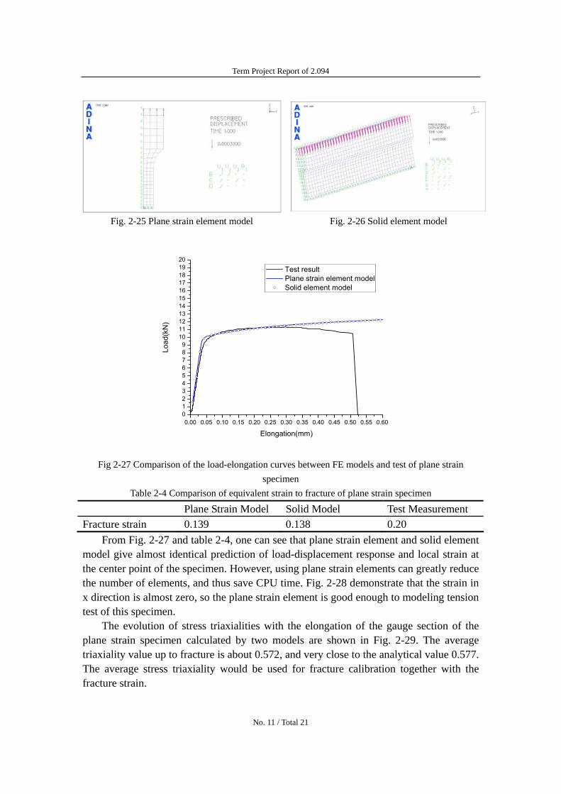
Term Project Report of 2094
Fig 2-25 Plane strain element model Fig 2-26 Solid element model
20 19 Test result18 Plane strain element model17
Solid element model 16 15 14 13 12 11 10 9 8 7 6 5 4 3 2 1 0000 005 010 015 020 025 030 035 040 045 050 055 060
Elongation(mm)
Load
(kN
)
Fig 2-27 Comparison of the load-elongation curves between FE models and test of plane strain specimen
Table 2-4 Comparison of equivalent strain to fracture of plane strain specimen
Plane Strain Model Solid Model Test Measurement Fracture strain 0139 0138 020
From Fig 2-27 and table 2-4 one can see that plane strain element and solid element model give almost identical prediction of load-displacement response and local strain at the center point of the specimen However using plane strain elements can greatly reduce the number of elements and thus save CPU time Fig 2-28 demonstrate that the strain in x direction is almost zero so the plane strain element is good enough to modeling tension test of this specimen
The evolution of stress triaxialities with the elongation of the gauge section of the plane strain specimen calculated by two models are shown in Fig 2-29 The average triaxiality value up to fracture is about 0572 and very close to the analytical value 0577 The average stress triaxiality would be used for fracture calibration together with the fracture strain
No 11 Total 21
Term Project Report of 2094
Fig 2-28 The band plot of the strain in XX direction
Plane strain element model
Stre
ss T
riaxi
ality
060
056
052
048
Solid element model
Fracture
01 02 03 04 05 06
Elongation(mm)
Fig 2-29 Evolution of stress triaxility of the flat grooved plane strain specimen
24 Punch indentation tests on circular disks This test provides information on fraction under the equi-biaxial state of stress
The most highly stressed point is located at the apex of the dome where the components of radial and circumferential stress and strain are equal to each other The disk specimens were secured to the 100mm diameter die by a heavy flange with 8 bolts The radius of the hemi-spherical punch was 45mm The load-displacement characteristics were recorded in the tests The measured displacement to fracture in our case was 274mm The tests were interrupted right after formation of nearly straight crack shown as shown in Fig 2-30
Accordingly a FE model of this test was built in ADINA with 4-node axisymmetric elements which is shown in Fig 2-31 The mesh edge length is 1mm The edge nodes of the disk model were fixed at all degree of freedom the center nodes of the disk model were given a symmetric boundary condition and the punch surface was given a prescribed downward displacement The contact surface on the punch was modeled as rigid and the friction coefficient is set to 001 The pressuredisplacement mixed interpolation function was used for this model to get better stress triaxiality prediction the difference between displacement-based and up mixed element will be discussed in
No 12 Total 21
Term Project Report of 2094
section 3 The time step was set to 0005s The deformation and the effective strain distribution of the disk were shown in Fig 2-32
Fig 2-30 A view of the fractured disk Fig 2-31 Numerical model of the punch test
Fig 2-32 Deformation and distribution of the disk specimen calculated by ADINA
The force displacement response can be obtained by plotting the reaction force on the punch and the displacement of the punch The comparison of the force displacement response between simulation and test result is shown in Fig 2-33 There is an excellent agreement of the measured load-displacement curve with the numerical model Also the history of the effective strain and stress triaxiality of the outer element at the apex of the dome was shown in Fig 2-34 from which one can obtain the equivalent strain to fracture of this specimen and the average stress triaxiality up to fracture of the fracture initiation point (apex of the dome) For the case of our aluminum sheet the calculated fracture strain is 063 which is very close to the strain value 069 from the measurement of thickness reduction after test The average triaxiality value up to fracture is about 065 and very close to the analytical value 23 The average stress triaxiality would be used for
No 13 Total 21
Term Project Report of 2094
fracture calibration together with the fracture strain 063
100
Forc
e(kN
)
90
80
70
60
50
40
30
20
10
0
Test result Numerical simulation
0 5 10 15 20 25 30 35
Displacement(mm)
Fig2-33 Comparison of the force displacement response of a punch test between test result and simulation output
00
02
04
06
08
10
12
14
16
18
20
Stre
ss T
riaxi
ality
Equi
vale
nt P
last
ic S
train
Equivalent plstic strain Stress triaxiality
Fracture
0 2 4 6 8 10 12 14 16 18 20 22 24 26 28 30 32 34 36 38 40
Displacement (mm)
Fig 2-34 Evolution of equivalent plastic strain and stress triaxiality at the fracture initiation point
25 Ductile fracture calibration using simulation results As all the numerical simulations of calibration tests has been performed and validated
by experimental results a fracture locus of our aluminum sheets can be calibrated with the simulation results Table 2-5 shows all the fracture points obtained from the numerical simulation
Table 2-5 Fracture points obtained from numerical simulations Point Specimen Type Stress Triaxiality Fracture Strain
1 Dog-bone 0345 048 2 Flat with cutouts 051 021 3 Flat grooved 0572 014 4 Punch indentation 065 063
No 14 Total 21
Term Project Report of 2094
A Mohr-Coulomb fracture criterion was used to calibrate the fracture locus of this aluminum sheet The form of this fracture criterion in the space of fracture strain and stress triaxiality is as followed
minus1
ε f = ⎨⎪⎧
⎪⎩cA 2
f3 ⎢⎡
⎣⎢⎜⎛
⎝⎜
1+ 3 c1
2
sdot f1 ⎟⎞⎟⎠+ c1
⎛⎜⎝η +
f 3
2 ⎞⎟⎠⎥⎤
⎥⎦
⎪⎬⎫
⎭⎪
n
(2-3)
where the functions f1 f2 and f3 are defined as
f1 1 27 η η 2 = cos arcsin ⎢
⎡minus ( minus 1)⎤⎥3 ⎣ 2 3 ⎦
( 2f2 = sin 1 arcsin ⎡minus 27 η η minus 1)⎤ (2-4) 3 ⎣⎢ 2 3 ⎥⎦
f3 c3 3 (1minus c3)( 1 minus1)= +
2 minus 3 f1
This fracture criterion is a function of equivalent strain to fracture ε f in terms of the
average stress triaxiality η up to fracture A and n are the material parameters in Eq
(2-1) This criterion has 3 calibration parameters c1c2 and c3 Hence points 1 3 and 4 in table 2-5 were used to calibrate the 3 free parameters while point 2 was used to validate the accuracy of the fracture locus The calibrated fracture locus is shown in Fig 2-35 One can see that the calibrated fracture locus can predict the fracture strain at point 2 (flat specimen with side cutouts) with good accuracy Therefore this fracture locus can be implemented into the FE codes to predict ductile fracture during calculations
c1=0154 c2=248MPa c3=098 A=438MPa n=007
Calibration Points
Validation Point
Fig2-35 Calibrated fracture locus of our aluminum sheets with numerical results
No 15 Total 21
Term Project Report of 2094
3 Parametric Study of Some Numerical Simulation Parameters To predict the initial crack position accurately the local strain and stress triaxiality are
very important to the fracture identification However some parameters may affect the local strainstress significantly such as number of integration points (NIP) through thickness element type mesh size and so on
Several finite element models were built based on the benchmark models in section 2 to study these effects The force-displacement response effective strain and stress triaxilality history at the initial crack position were compared and analyzed
31 Effect of Number of Integration Point through thickness (NIP) This study is based on the shell element model of the flat specimen with cutouts The
benchmark model in section 22 is with 5 integration points though thickness and the Gauss integration was used Two more shell element models of the flat specimen with cutouts with 2 and 3 through thickness integration points respectively were built in ADINA
As is shown in Fig 3-1 as the NIP through thickness of shell elements increases the load-elongation response predicted by the numerical model is closer to the experimental results From Fig 3-2 and 3-3 one can see that the local strain and stress triaxiality at the crack initiation point (the center of the specimen) predicted by the 2 NIP model are much lower than the 5 NIP model which has shown good accuracy in section 22 Hence if shell elements are used for numerical simulations of similar problems at least 5 through thickness integration points should be employed
Load
(kN
)
17 16 15 14 13 12 11 10 9 8 7 6 5 4 3 2 1 0
Test INP=2 INP=3 INP=5
Fracture
00 01 02 03 04 05 06 07 08 09 10 11 12 13 14 15
Elongation(mm)
Fig 3-1 Load-elongation responses of three models with different NIP through thickness
No 16 Total 21
Term Project Report of 2094
Equ
ival
ent P
last
ic S
train
10
09
08
07
06
05
04
03
02
01
00
INP=2 INP=3 INP=5
Fracture
00 02 04 06 08 10 12 14 16 18 20
Elongation(mm)
Fig 3-2 Strain history at crack initiation point of three models with different NIP through thickness
044
046
048
050
052
054
056
058
Stre
ss T
riaxi
ality
NIP=2 NIP=3 NIP=5
Fracture
02 04 06 08 10 12 14
Elongation(mm)
Fig 3-3 Stress triaxiality history at crack initiation point of three models with different NIP through thickness
32 Effect of element type This study is based on the model of punch indentation tests in section 24 Three
different models with different element types and interpolation formulations were
No 17 Total 21
Term Project Report of 2094
compared in this section displacement based 4-node element mixed 41 and 93 up element
From Fig3-4 and Fig 3-5 one can see that the force-displacement response and local strain evolution at the crack initiation point (the apex of the dome) are not affected much by the element type However as is shown in Fig 3-6 the displacement based element can not predict the stress triaxiality well because the analytical stress triaxiality value should be 23 in this test Since stress triaxiality is a normalized pressure the low accuracy triaxiality prediction is due to the unreasonable pressure distribution and magnitudes predicted by the displacement-based elements as is shown in Fig 3-7 The pressure distribution calculated by mixed up elements are much more accurate as is shown in Fig 3-8
Test 4-node displacement based element 41 mixed up element 93 mixed up element
Fracture
0 5 10 15 20 25 30 35 40 45 50
Displacement(mm)
Equ
ival
ent P
last
ic S
train
07
06
05
04
03
02
01
0 2 4 6 8 10 12 14 16 18 20 22 24 26 28
4-node displacement based element 41 mixed up element 93 mixed up element
Fracture
120
110
100
90
80
Forc
e(kN
)
70
60
50
40
30
20
10
0 00
Displacement(mm)
Fig 3-4 Force-displacement responses of 3 models Fig 3-5 Equivalent plastic strain evolution at crack with different element types initiation point of 3 models with different element
types
10
05
00
4-node displacment based elment 41 mixed up element 93 mixed up element
-05
-10
-15
-20
-25
-30
-35
-40
-45
-50
Stre
ss T
riaxi
ality
0 5 10 15 20 25 30
Displacement(mm)
Fig 3-6 Evolution of stress triaxiality at crack initiation point of 3 element types
No 18 Total 21
Term Project Report of 2094
Fig 3-7 Pressure distribution of the model with 4 node Fig 3-8 Pressure distribution of the model with 93 displacement based elments mixed elements
33 Mesh size effect This study is based on the model of punch indentation tests in section 24 Three
different models with different mesh sizes were built as is shown in Fig 3-9 and the force-displacement responses local strain and stress triaxiality history at the crach initiation point (the apex of the dome) were compared and studied The 3 different mesh edge length studied in this section was 1mm 05mm and 2mm The 41 mixed up elements were employed in all three models
Fig 3-10 and 3-11 show that the force-displacement response and stress triaxiality predicted by the numerical models become closer to the experimental result or analytical result as the mesh goes finer As is shown by Fig 3-12 the local strain seems to be larger as the mesh edge length is smaller in the early stage but it reach convergence finally Hence the finite element model is convergent as the mesh becomes finer
(a)Mesh edge length=1mm (b)Mesh edge length=05mm (c)Mesh edge length=2mm Fig 3-9 Three models with different mesh size
No 19 Total 21
Term Project Report of 2094
Test Mesh edge length=1mm 08
Mesh edge length=1mm Mesh edge length=2mm Mesh edge length=05mm
Mesh edge length=05mm Mesh edge length=2mm
120
110
100
07
06 90
80
Stre
ss T
riaxi
ality
05
04
03 Forc
e(kN
)
70
60
50
40
30
20
02
01
00
10
0 0 5 10 15 20 25 30 35 40 45 50 0 5 10 15 20 25 30 35 40 45 50
Displacement(mm) Displacement(mm)
Fig 3-10 Force-displacement responses of 3 models Fig 3-11 Evolution of stress triaxiality at crack with different element size initiation point of 3 models with different element size
10
Mesh edge length=1mm 08 Mesh edge length=05mm Mesh edge length=2mm
Equi
vale
nt P
lstic
Stra
in
06
04
02
00 0 5 10 15 20 25 30
Displacement(mm)
Fig 3-12 Equivalent plastic strain evolution at crack initiation point of 3 models with different element size
No 20 Total 21
Term Project Report of 2094
4 Conclusions In this project four types of specimens made from our aluminum sheets were tested
in the lab to investigate the fracture characteristics of this material At the same time corresponding finite element models were built to simulate the fracture calibration tests Most suited model for each test was determined after comparisons and analysis and the fracture locus of this material was calibrated with the simulation results Moreover a brief parametric study was performed to evaluate the effect of several FE parameters on the numerical simulation results Main conclusions are shown as followed
1) Finite element model can simulate the physical problems very well Suited FE models can predict the load-displacement responses local strain and stress with good accuracy
2) Selection of element type and modeling strategy should depend on the geometry and boundary conditions of the physical problem For this project one should choose solid elements for dog-bone specimen shell elements for flat specimen with cutouts plane strain elements for flat grooved specimen and axisymmetric elements for the punch indentation test
3) Number of integration points (NIP) through thickness has a great effect on the strain and stress distribution of shell elements Once the through thickness stress gradient is involved in a physical problem such as necking or bending a larger NIP through thickness should be employed
4) The up mixed element can predict the pressure distribution and magnitude much more accurate
5) The FE models in this project are convergent As the mesh becomes finer both the load-displacement response and local stressstrain output become closer to experimental results or analytical values
No 21 Total 21
MIT OpenCourseWare httpocwmitedu
2094 Finite Element Analysis of Solids and Fluids IISpring 2011
For information about citing these materials or our Terms of Use visit httpocwmiteduterms
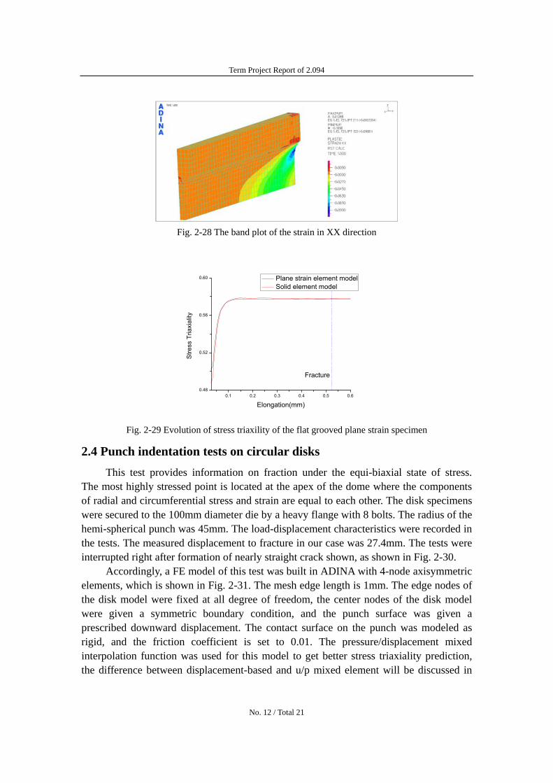
Term Project Report of 2094
Fig 2-28 The band plot of the strain in XX direction
Plane strain element model
Stre
ss T
riaxi
ality
060
056
052
048
Solid element model
Fracture
01 02 03 04 05 06
Elongation(mm)
Fig 2-29 Evolution of stress triaxility of the flat grooved plane strain specimen
24 Punch indentation tests on circular disks This test provides information on fraction under the equi-biaxial state of stress
The most highly stressed point is located at the apex of the dome where the components of radial and circumferential stress and strain are equal to each other The disk specimens were secured to the 100mm diameter die by a heavy flange with 8 bolts The radius of the hemi-spherical punch was 45mm The load-displacement characteristics were recorded in the tests The measured displacement to fracture in our case was 274mm The tests were interrupted right after formation of nearly straight crack shown as shown in Fig 2-30
Accordingly a FE model of this test was built in ADINA with 4-node axisymmetric elements which is shown in Fig 2-31 The mesh edge length is 1mm The edge nodes of the disk model were fixed at all degree of freedom the center nodes of the disk model were given a symmetric boundary condition and the punch surface was given a prescribed downward displacement The contact surface on the punch was modeled as rigid and the friction coefficient is set to 001 The pressuredisplacement mixed interpolation function was used for this model to get better stress triaxiality prediction the difference between displacement-based and up mixed element will be discussed in
No 12 Total 21
Term Project Report of 2094
section 3 The time step was set to 0005s The deformation and the effective strain distribution of the disk were shown in Fig 2-32
Fig 2-30 A view of the fractured disk Fig 2-31 Numerical model of the punch test
Fig 2-32 Deformation and distribution of the disk specimen calculated by ADINA
The force displacement response can be obtained by plotting the reaction force on the punch and the displacement of the punch The comparison of the force displacement response between simulation and test result is shown in Fig 2-33 There is an excellent agreement of the measured load-displacement curve with the numerical model Also the history of the effective strain and stress triaxiality of the outer element at the apex of the dome was shown in Fig 2-34 from which one can obtain the equivalent strain to fracture of this specimen and the average stress triaxiality up to fracture of the fracture initiation point (apex of the dome) For the case of our aluminum sheet the calculated fracture strain is 063 which is very close to the strain value 069 from the measurement of thickness reduction after test The average triaxiality value up to fracture is about 065 and very close to the analytical value 23 The average stress triaxiality would be used for
No 13 Total 21
Term Project Report of 2094
fracture calibration together with the fracture strain 063
100
Forc
e(kN
)
90
80
70
60
50
40
30
20
10
0
Test result Numerical simulation
0 5 10 15 20 25 30 35
Displacement(mm)
Fig2-33 Comparison of the force displacement response of a punch test between test result and simulation output
00
02
04
06
08
10
12
14
16
18
20
Stre
ss T
riaxi
ality
Equi
vale
nt P
last
ic S
train
Equivalent plstic strain Stress triaxiality
Fracture
0 2 4 6 8 10 12 14 16 18 20 22 24 26 28 30 32 34 36 38 40
Displacement (mm)
Fig 2-34 Evolution of equivalent plastic strain and stress triaxiality at the fracture initiation point
25 Ductile fracture calibration using simulation results As all the numerical simulations of calibration tests has been performed and validated
by experimental results a fracture locus of our aluminum sheets can be calibrated with the simulation results Table 2-5 shows all the fracture points obtained from the numerical simulation
Table 2-5 Fracture points obtained from numerical simulations Point Specimen Type Stress Triaxiality Fracture Strain
1 Dog-bone 0345 048 2 Flat with cutouts 051 021 3 Flat grooved 0572 014 4 Punch indentation 065 063
No 14 Total 21
Term Project Report of 2094
A Mohr-Coulomb fracture criterion was used to calibrate the fracture locus of this aluminum sheet The form of this fracture criterion in the space of fracture strain and stress triaxiality is as followed
minus1
ε f = ⎨⎪⎧
⎪⎩cA 2
f3 ⎢⎡
⎣⎢⎜⎛
⎝⎜
1+ 3 c1
2
sdot f1 ⎟⎞⎟⎠+ c1
⎛⎜⎝η +
f 3
2 ⎞⎟⎠⎥⎤
⎥⎦
⎪⎬⎫
⎭⎪
n
(2-3)
where the functions f1 f2 and f3 are defined as
f1 1 27 η η 2 = cos arcsin ⎢
⎡minus ( minus 1)⎤⎥3 ⎣ 2 3 ⎦
( 2f2 = sin 1 arcsin ⎡minus 27 η η minus 1)⎤ (2-4) 3 ⎣⎢ 2 3 ⎥⎦
f3 c3 3 (1minus c3)( 1 minus1)= +
2 minus 3 f1
This fracture criterion is a function of equivalent strain to fracture ε f in terms of the
average stress triaxiality η up to fracture A and n are the material parameters in Eq
(2-1) This criterion has 3 calibration parameters c1c2 and c3 Hence points 1 3 and 4 in table 2-5 were used to calibrate the 3 free parameters while point 2 was used to validate the accuracy of the fracture locus The calibrated fracture locus is shown in Fig 2-35 One can see that the calibrated fracture locus can predict the fracture strain at point 2 (flat specimen with side cutouts) with good accuracy Therefore this fracture locus can be implemented into the FE codes to predict ductile fracture during calculations
c1=0154 c2=248MPa c3=098 A=438MPa n=007
Calibration Points
Validation Point
Fig2-35 Calibrated fracture locus of our aluminum sheets with numerical results
No 15 Total 21
Term Project Report of 2094
3 Parametric Study of Some Numerical Simulation Parameters To predict the initial crack position accurately the local strain and stress triaxiality are
very important to the fracture identification However some parameters may affect the local strainstress significantly such as number of integration points (NIP) through thickness element type mesh size and so on
Several finite element models were built based on the benchmark models in section 2 to study these effects The force-displacement response effective strain and stress triaxilality history at the initial crack position were compared and analyzed
31 Effect of Number of Integration Point through thickness (NIP) This study is based on the shell element model of the flat specimen with cutouts The
benchmark model in section 22 is with 5 integration points though thickness and the Gauss integration was used Two more shell element models of the flat specimen with cutouts with 2 and 3 through thickness integration points respectively were built in ADINA
As is shown in Fig 3-1 as the NIP through thickness of shell elements increases the load-elongation response predicted by the numerical model is closer to the experimental results From Fig 3-2 and 3-3 one can see that the local strain and stress triaxiality at the crack initiation point (the center of the specimen) predicted by the 2 NIP model are much lower than the 5 NIP model which has shown good accuracy in section 22 Hence if shell elements are used for numerical simulations of similar problems at least 5 through thickness integration points should be employed
Load
(kN
)
17 16 15 14 13 12 11 10 9 8 7 6 5 4 3 2 1 0
Test INP=2 INP=3 INP=5
Fracture
00 01 02 03 04 05 06 07 08 09 10 11 12 13 14 15
Elongation(mm)
Fig 3-1 Load-elongation responses of three models with different NIP through thickness
No 16 Total 21
Term Project Report of 2094
Equ
ival
ent P
last
ic S
train
10
09
08
07
06
05
04
03
02
01
00
INP=2 INP=3 INP=5
Fracture
00 02 04 06 08 10 12 14 16 18 20
Elongation(mm)
Fig 3-2 Strain history at crack initiation point of three models with different NIP through thickness
044
046
048
050
052
054
056
058
Stre
ss T
riaxi
ality
NIP=2 NIP=3 NIP=5
Fracture
02 04 06 08 10 12 14
Elongation(mm)
Fig 3-3 Stress triaxiality history at crack initiation point of three models with different NIP through thickness
32 Effect of element type This study is based on the model of punch indentation tests in section 24 Three
different models with different element types and interpolation formulations were
No 17 Total 21
Term Project Report of 2094
compared in this section displacement based 4-node element mixed 41 and 93 up element
From Fig3-4 and Fig 3-5 one can see that the force-displacement response and local strain evolution at the crack initiation point (the apex of the dome) are not affected much by the element type However as is shown in Fig 3-6 the displacement based element can not predict the stress triaxiality well because the analytical stress triaxiality value should be 23 in this test Since stress triaxiality is a normalized pressure the low accuracy triaxiality prediction is due to the unreasonable pressure distribution and magnitudes predicted by the displacement-based elements as is shown in Fig 3-7 The pressure distribution calculated by mixed up elements are much more accurate as is shown in Fig 3-8
Test 4-node displacement based element 41 mixed up element 93 mixed up element
Fracture
0 5 10 15 20 25 30 35 40 45 50
Displacement(mm)
Equ
ival
ent P
last
ic S
train
07
06
05
04
03
02
01
0 2 4 6 8 10 12 14 16 18 20 22 24 26 28
4-node displacement based element 41 mixed up element 93 mixed up element
Fracture
120
110
100
90
80
Forc
e(kN
)
70
60
50
40
30
20
10
0 00
Displacement(mm)
Fig 3-4 Force-displacement responses of 3 models Fig 3-5 Equivalent plastic strain evolution at crack with different element types initiation point of 3 models with different element
types
10
05
00
4-node displacment based elment 41 mixed up element 93 mixed up element
-05
-10
-15
-20
-25
-30
-35
-40
-45
-50
Stre
ss T
riaxi
ality
0 5 10 15 20 25 30
Displacement(mm)
Fig 3-6 Evolution of stress triaxiality at crack initiation point of 3 element types
No 18 Total 21
Term Project Report of 2094
Fig 3-7 Pressure distribution of the model with 4 node Fig 3-8 Pressure distribution of the model with 93 displacement based elments mixed elements
33 Mesh size effect This study is based on the model of punch indentation tests in section 24 Three
different models with different mesh sizes were built as is shown in Fig 3-9 and the force-displacement responses local strain and stress triaxiality history at the crach initiation point (the apex of the dome) were compared and studied The 3 different mesh edge length studied in this section was 1mm 05mm and 2mm The 41 mixed up elements were employed in all three models
Fig 3-10 and 3-11 show that the force-displacement response and stress triaxiality predicted by the numerical models become closer to the experimental result or analytical result as the mesh goes finer As is shown by Fig 3-12 the local strain seems to be larger as the mesh edge length is smaller in the early stage but it reach convergence finally Hence the finite element model is convergent as the mesh becomes finer
(a)Mesh edge length=1mm (b)Mesh edge length=05mm (c)Mesh edge length=2mm Fig 3-9 Three models with different mesh size
No 19 Total 21
Term Project Report of 2094
Test Mesh edge length=1mm 08
Mesh edge length=1mm Mesh edge length=2mm Mesh edge length=05mm
Mesh edge length=05mm Mesh edge length=2mm
120
110
100
07
06 90
80
Stre
ss T
riaxi
ality
05
04
03 Forc
e(kN
)
70
60
50
40
30
20
02
01
00
10
0 0 5 10 15 20 25 30 35 40 45 50 0 5 10 15 20 25 30 35 40 45 50
Displacement(mm) Displacement(mm)
Fig 3-10 Force-displacement responses of 3 models Fig 3-11 Evolution of stress triaxiality at crack with different element size initiation point of 3 models with different element size
10
Mesh edge length=1mm 08 Mesh edge length=05mm Mesh edge length=2mm
Equi
vale
nt P
lstic
Stra
in
06
04
02
00 0 5 10 15 20 25 30
Displacement(mm)
Fig 3-12 Equivalent plastic strain evolution at crack initiation point of 3 models with different element size
No 20 Total 21
Term Project Report of 2094
4 Conclusions In this project four types of specimens made from our aluminum sheets were tested
in the lab to investigate the fracture characteristics of this material At the same time corresponding finite element models were built to simulate the fracture calibration tests Most suited model for each test was determined after comparisons and analysis and the fracture locus of this material was calibrated with the simulation results Moreover a brief parametric study was performed to evaluate the effect of several FE parameters on the numerical simulation results Main conclusions are shown as followed
1) Finite element model can simulate the physical problems very well Suited FE models can predict the load-displacement responses local strain and stress with good accuracy
2) Selection of element type and modeling strategy should depend on the geometry and boundary conditions of the physical problem For this project one should choose solid elements for dog-bone specimen shell elements for flat specimen with cutouts plane strain elements for flat grooved specimen and axisymmetric elements for the punch indentation test
3) Number of integration points (NIP) through thickness has a great effect on the strain and stress distribution of shell elements Once the through thickness stress gradient is involved in a physical problem such as necking or bending a larger NIP through thickness should be employed
4) The up mixed element can predict the pressure distribution and magnitude much more accurate
5) The FE models in this project are convergent As the mesh becomes finer both the load-displacement response and local stressstrain output become closer to experimental results or analytical values
No 21 Total 21
MIT OpenCourseWare httpocwmitedu
2094 Finite Element Analysis of Solids and Fluids IISpring 2011
For information about citing these materials or our Terms of Use visit httpocwmiteduterms
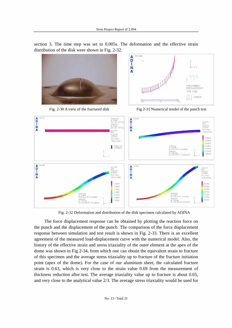
Term Project Report of 2094
Equ
ival
ent P
last
ic S
train
10
09
08
07
06
05
04
03
02
01
00
INP=2 INP=3 INP=5
Fracture
00 02 04 06 08 10 12 14 16 18 20
Elongation(mm)
Fig 3-2 Strain history at crack initiation point of three models with different NIP through thickness
044
046
048
050
052
054
056
058
Stre
ss T
riaxi
ality
NIP=2 NIP=3 NIP=5
Fracture
02 04 06 08 10 12 14
Elongation(mm)
Fig 3-3 Stress triaxiality history at crack initiation point of three models with different NIP through thickness
32 Effect of element type This study is based on the model of punch indentation tests in section 24 Three
different models with different element types and interpolation formulations were
No 17 Total 21
Term Project Report of 2094
compared in this section displacement based 4-node element mixed 41 and 93 up element
From Fig3-4 and Fig 3-5 one can see that the force-displacement response and local strain evolution at the crack initiation point (the apex of the dome) are not affected much by the element type However as is shown in Fig 3-6 the displacement based element can not predict the stress triaxiality well because the analytical stress triaxiality value should be 23 in this test Since stress triaxiality is a normalized pressure the low accuracy triaxiality prediction is due to the unreasonable pressure distribution and magnitudes predicted by the displacement-based elements as is shown in Fig 3-7 The pressure distribution calculated by mixed up elements are much more accurate as is shown in Fig 3-8
Test 4-node displacement based element 41 mixed up element 93 mixed up element
Fracture
0 5 10 15 20 25 30 35 40 45 50
Displacement(mm)
Equ
ival
ent P
last
ic S
train
07
06
05
04
03
02
01
0 2 4 6 8 10 12 14 16 18 20 22 24 26 28
4-node displacement based element 41 mixed up element 93 mixed up element
Fracture
120
110
100
90
80
Forc
e(kN
)
70
60
50
40
30
20
10
0 00
Displacement(mm)
Fig 3-4 Force-displacement responses of 3 models Fig 3-5 Equivalent plastic strain evolution at crack with different element types initiation point of 3 models with different element
types
10
05
00
4-node displacment based elment 41 mixed up element 93 mixed up element
-05
-10
-15
-20
-25
-30
-35
-40
-45
-50
Stre
ss T
riaxi
ality
0 5 10 15 20 25 30
Displacement(mm)
Fig 3-6 Evolution of stress triaxiality at crack initiation point of 3 element types
No 18 Total 21
Term Project Report of 2094
Fig 3-7 Pressure distribution of the model with 4 node Fig 3-8 Pressure distribution of the model with 93 displacement based elments mixed elements
33 Mesh size effect This study is based on the model of punch indentation tests in section 24 Three
different models with different mesh sizes were built as is shown in Fig 3-9 and the force-displacement responses local strain and stress triaxiality history at the crach initiation point (the apex of the dome) were compared and studied The 3 different mesh edge length studied in this section was 1mm 05mm and 2mm The 41 mixed up elements were employed in all three models
Fig 3-10 and 3-11 show that the force-displacement response and stress triaxiality predicted by the numerical models become closer to the experimental result or analytical result as the mesh goes finer As is shown by Fig 3-12 the local strain seems to be larger as the mesh edge length is smaller in the early stage but it reach convergence finally Hence the finite element model is convergent as the mesh becomes finer
(a)Mesh edge length=1mm (b)Mesh edge length=05mm (c)Mesh edge length=2mm Fig 3-9 Three models with different mesh size
No 19 Total 21
Term Project Report of 2094
Test Mesh edge length=1mm 08
Mesh edge length=1mm Mesh edge length=2mm Mesh edge length=05mm
Mesh edge length=05mm Mesh edge length=2mm
120
110
100
07
06 90
80
Stre
ss T
riaxi
ality
05
04
03 Forc
e(kN
)
70
60
50
40
30
20
02
01
00
10
0 0 5 10 15 20 25 30 35 40 45 50 0 5 10 15 20 25 30 35 40 45 50
Displacement(mm) Displacement(mm)
Fig 3-10 Force-displacement responses of 3 models Fig 3-11 Evolution of stress triaxiality at crack with different element size initiation point of 3 models with different element size
10
Mesh edge length=1mm 08 Mesh edge length=05mm Mesh edge length=2mm
Equi
vale
nt P
lstic
Stra
in
06
04
02
00 0 5 10 15 20 25 30
Displacement(mm)
Fig 3-12 Equivalent plastic strain evolution at crack initiation point of 3 models with different element size
No 20 Total 21
Term Project Report of 2094
4 Conclusions In this project four types of specimens made from our aluminum sheets were tested
in the lab to investigate the fracture characteristics of this material At the same time corresponding finite element models were built to simulate the fracture calibration tests Most suited model for each test was determined after comparisons and analysis and the fracture locus of this material was calibrated with the simulation results Moreover a brief parametric study was performed to evaluate the effect of several FE parameters on the numerical simulation results Main conclusions are shown as followed
1) Finite element model can simulate the physical problems very well Suited FE models can predict the load-displacement responses local strain and stress with good accuracy
2) Selection of element type and modeling strategy should depend on the geometry and boundary conditions of the physical problem For this project one should choose solid elements for dog-bone specimen shell elements for flat specimen with cutouts plane strain elements for flat grooved specimen and axisymmetric elements for the punch indentation test
3) Number of integration points (NIP) through thickness has a great effect on the strain and stress distribution of shell elements Once the through thickness stress gradient is involved in a physical problem such as necking or bending a larger NIP through thickness should be employed
4) The up mixed element can predict the pressure distribution and magnitude much more accurate
5) The FE models in this project are convergent As the mesh becomes finer both the load-displacement response and local stressstrain output become closer to experimental results or analytical values
No 21 Total 21
MIT OpenCourseWare httpocwmitedu
2094 Finite Element Analysis of Solids and Fluids IISpring 2011
For information about citing these materials or our Terms of Use visit httpocwmiteduterms

Term Project Report of 2094
Test Mesh edge length=1mm 08
Mesh edge length=1mm Mesh edge length=2mm Mesh edge length=05mm
Mesh edge length=05mm Mesh edge length=2mm
120
110
100
07
06 90
80
Stre
ss T
riaxi
ality
05
04
03 Forc
e(kN
)
70
60
50
40
30
20
02
01
00
10
0 0 5 10 15 20 25 30 35 40 45 50 0 5 10 15 20 25 30 35 40 45 50
Displacement(mm) Displacement(mm)
Fig 3-10 Force-displacement responses of 3 models Fig 3-11 Evolution of stress triaxiality at crack with different element size initiation point of 3 models with different element size
10
Mesh edge length=1mm 08 Mesh edge length=05mm Mesh edge length=2mm
Equi
vale
nt P
lstic
Stra
in
06
04
02
00 0 5 10 15 20 25 30
Displacement(mm)
Fig 3-12 Equivalent plastic strain evolution at crack initiation point of 3 models with different element size
No 20 Total 21
Term Project Report of 2094
4 Conclusions In this project four types of specimens made from our aluminum sheets were tested
in the lab to investigate the fracture characteristics of this material At the same time corresponding finite element models were built to simulate the fracture calibration tests Most suited model for each test was determined after comparisons and analysis and the fracture locus of this material was calibrated with the simulation results Moreover a brief parametric study was performed to evaluate the effect of several FE parameters on the numerical simulation results Main conclusions are shown as followed
1) Finite element model can simulate the physical problems very well Suited FE models can predict the load-displacement responses local strain and stress with good accuracy
2) Selection of element type and modeling strategy should depend on the geometry and boundary conditions of the physical problem For this project one should choose solid elements for dog-bone specimen shell elements for flat specimen with cutouts plane strain elements for flat grooved specimen and axisymmetric elements for the punch indentation test
3) Number of integration points (NIP) through thickness has a great effect on the strain and stress distribution of shell elements Once the through thickness stress gradient is involved in a physical problem such as necking or bending a larger NIP through thickness should be employed
4) The up mixed element can predict the pressure distribution and magnitude much more accurate
5) The FE models in this project are convergent As the mesh becomes finer both the load-displacement response and local stressstrain output become closer to experimental results or analytical values
No 21 Total 21
MIT OpenCourseWare httpocwmitedu
2094 Finite Element Analysis of Solids and Fluids IISpring 2011
For information about citing these materials or our Terms of Use visit httpocwmiteduterms

MIT OpenCourseWare httpocwmitedu
2094 Finite Element Analysis of Solids and Fluids IISpring 2011
For information about citing these materials or our Terms of Use visit httpocwmiteduterms
Related Documents