Overview The count model, from scratch What is a GAM? What is smoothing? Fitting GAMs using dsm 2 / 37 Building a model, from scratch Know count in segment 3 / 37 Building a model, from scratch Know count in segment Want : 4 / 37 Building a model, from scratch Know count in segment Want : How to build ? 5 / 37 Building a model, from scratch Know count in segment Want : How to build ? Additive model of smooths : is the link function 6 / 37 Building a model, from scratch What about area and detectability? area of segment - "offset" probability of detection in segment 7 / 37 Building a model, from scratch It's a statistical model so: has a distribution (count) are residuals (differences between model and observations) 8 / 37 That's a Generalized Additive Model! That's a Generalized Additive Model! 9 / 37 9 / 37 Now let's look at each bit... Now let's look at each bit... 10 / 37 10 / 37 Response where 11 / 37 Response is a count Often, it's mostly zero mean variance (Poisson isn't good at this) Count distributions 12 / 37 (NB there is a point mass at zero not plotted) Poisson is We estimate: (p in R), "power" parameter (Scale est. in R), scale parameter Tweedie distribution 13 / 37 Estimate No scale parameter (Scale est.=1 always) (Poisson: ) Negative binomial distribution 14 / 37 Smooths 15 / 37 Think =smooth Want a line that is "close" to all the data Balance between interpolation and "fit" What about these "s" things? 16 / 37 What is smoothing? What is smoothing? 17 / 37 17 / 37 Smoothing We think underlying phenomenon is smooth "Abundance is a smooth function of depth" 1, 2 or more dimensions 18 / 37 We set: "type": bases (made up of basis functions) "maximum wigglyness": basis size (sometimes: dimension/complexity) Automatically estimate: "how wiggly it needs to be": smoothing parameter(s) Estimating smooths 19 / 37 Splines Functions made of other, simpler functions Basis functions , estimate 20 / 37 Thinking about wigglyness Visually: Lots of wiggles not smooth Straight line very smooth Smoothing parameter ( ) controls this 21 / 37 How wiggly are things? Measure the effective degrees of freedom (EDF) Set basis complexity or "size", Set "large enough" 22 / 37 I can't teach you all of GAMs in 1 week Good intro book (also a good textbook on GLMs and GLMMs) Quite technical in places More resources on course website dsm is based on mgcv by Simon Wood Getting more out of GAMs 23 / 37 Fitting GAMs using dsm Fitting GAMs using dsm 24 / 37 24 / 37 Translating maths into R where are some errors, count distribution inside the link: formula=count ~ s(y) response distribution: family=nb() or family=tw() detectability: ddf.obj=df_hr offset, data: segment.data=segs, observation.data=obs 25 / 37 Your rst DSM library(dsm) dsm_x_tw <- dsm(count~s(x), ddf.obj=df, segment.data=segs, observation.data=obs, family=tw()) 26 / 37 summary(dsm_x_tw) ## ## Family: Tweedie(p=1.326) ## Link function: log ## ## Formula: ## count ~ s(x) + offset(off.set) ## ## Parametric coefficients: ## Estimate Std. Error t value Pr(>|t|) ## (Intercept) -19.8115 0.2277 -87.01 <2e-16 *** ## --- ## Signif. codes: 0 '***' 0.001 '**' 0.01 '*' 0.05 '.' 0.1 ' ' 1 ## ## Approximate significance of smooth terms: ## edf Ref.df F p-value ## s(x) 4.962 6.047 6.403 1.79e-06 *** ## --- ## Signif. codes: 0 '***' 0.001 '**' 0.01 '*' 0.05 '.' 0.1 ' ' 1 ## ## R-sq.(adj) = 0.0283 Deviance explained = 17.9% ## -REML = 409.94 Scale est. = 6.0413 n = 949 27 / 37 plot(dsm_x_tw) Dashed lines indicate +/- 2 standard errors Rug plot On the link scale EDF on axis Plotting 28 / 37 Adding a term Just use + dsm_xy_tw <- dsm(count ~ s(x) + s(y), ddf.obj=df, segment.data=segs, observation.data=obs, family=tw()) 29 / 37 summary(dsm_xy_tw) ## ## Family: Tweedie(p=1.306) ## Link function: log ## ## Formula: ## count ~ s(x) + s(y) + offset(off.set) ## ## Parametric coefficients: ## Estimate Std. Error t value Pr(>|t|) ## (Intercept) -20.0908 0.2381 -84.39 <2e-16 *** ## --- ## Signif. codes: 0 '***' 0.001 '**' 0.01 '*' 0.05 '.' 0.1 ' ' 1 ## ## Approximate significance of smooth terms: ## edf Ref.df F p-value ## s(x) 4.943 6.057 3.224 0.00425 ** ## s(y) 5.293 6.419 4.034 0.00033 *** ## --- ## Signif. codes: 0 '***' 0.001 '**' 0.01 '*' 0.05 '.' 0.1 ' ' 1 ## ## R-sq.(adj) = 0.0678 Deviance explained = 27.4% ## -REML = 399.84 Scale est. = 5.3157 n = 949 30 / 37 Plotting plot(dsm_xy_tw, pages=1) 31 / 37 Bivariate terms Assumed an additive structure No interaction We can specify s(x,y) (and s(x,y,z,...)) 32 / 37 Bivariate spatial term dsm_xyb_tw <- dsm(count ~ s(x, y), ddf.obj=df, segment.data=segs, observation.data=obs, family=tw()) 33 / 37 summary(dsm_xyb_tw) ## ## Family: Tweedie(p=1.29) ## Link function: log ## ## Formula: ## count ~ s(x, y) + offset(off.set) ## ## Parametric coefficients: ## Estimate Std. Error t value Pr(>|t|) ## (Intercept) -20.2745 0.2477 -81.85 <2e-16 *** ## --- ## Signif. codes: 0 '***' 0.001 '**' 0.01 '*' 0.05 '.' 0.1 ' ' 1 ## ## Approximate significance of smooth terms: ## edf Ref.df F p-value ## s(x,y) 16.89 21.12 4.333 <2e-16 *** ## --- ## Signif. codes: 0 '***' 0.001 '**' 0.01 '*' 0.05 '.' 0.1 ' ' 1 ## ## R-sq.(adj) = 0.102 Deviance explained = 34.7% ## -REML = 394.86 Scale est. = 4.8248 n = 949 34 / 37 plot(dsm_xyb_tw, select=1, scheme=2, asp=1) On link scale scheme=2 makes heatmap (set too.far to exclude points far from data) Plotting 35 / 37 Comparing bivariate and additive models 36 / 37 Let's have a go... Let's have a go... 37 / 37 37 / 37 Lecture 2 : Generalized Additive Models Lecture 2 : Generalized Additive Models 1 / 37 1 / 37

Welcome message from author
This document is posted to help you gain knowledge. Please leave a comment to let me know what you think about it! Share it to your friends and learn new things together.
Transcript

OverviewThe count model, from scratch
What is a GAM?
What is smoothing?
Fitting GAMs using dsm
2 / 37
Building a model, from scratchKnow count in segment 𝑛𝑗 𝑗
3 / 37
Building a model, from scratchKnow count in segment
Want :
𝑛𝑗 𝑗
= 𝑓([environmental covariates )𝑛𝑗 ]𝑗
4 / 37
Building a model, from scratchKnow count in segment
Want :
How to build ?
𝑛𝑗 𝑗
= 𝑓([environmental covariates )𝑛𝑗 ]𝑗
𝑓
5 / 37
Building a model, from scratchKnow count in segment
Want :
How to build ?
Additive model of smooths :
is the link function
𝑛𝑗 𝑗
= 𝑓([environmental covariates )𝑛𝑗 ]𝑗
𝑓
𝑠
= exp [ + 𝑠( ) + 𝑠( )]𝑛𝑗 𝛽0 y𝑗 Depth𝑗
model terms
exp
6 / 37
Building a model, from scratch
What about area and detectability?
area of segment - "offset"
probability of detection in segment
= exp [ + 𝑠( ) + 𝑠( )]𝑛𝑗 𝐴𝑗 �̂� 𝑗 𝛽0 y𝑗 Depth𝑗
𝐴𝑗
�̂� 𝑗
7 / 37
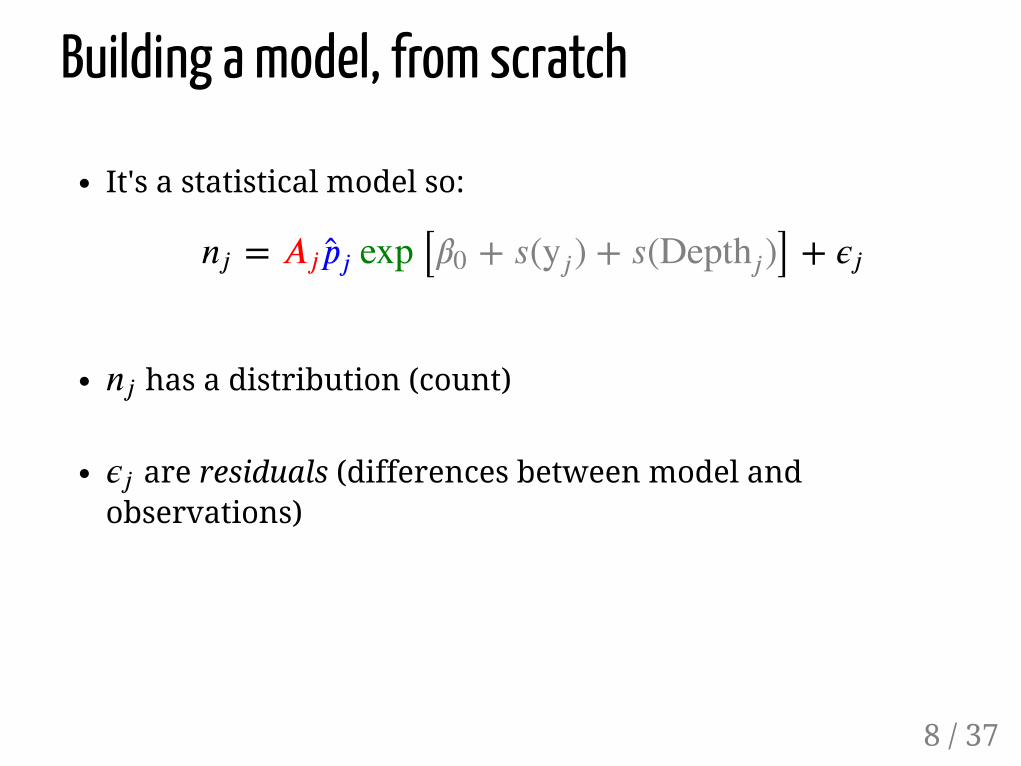
Building a model, from scratch
It's a statistical model so:
has a distribution (count)
are residuals (differences between model andobservations)
= exp [ + 𝑠( ) + 𝑠( )] +𝑛𝑗 𝐴𝑗 �̂� 𝑗 𝛽0 y𝑗 Depth𝑗 𝜖𝑗
𝑛𝑗
𝜖𝑗
8 / 37
That's a Generalized Additive Model!That's a Generalized Additive Model!
9 / 379 / 37
Now let's look at each bit...Now let's look at each bit...
10 / 3710 / 37
Response
where
= exp[ + 𝑠( ) + 𝑠( )] +𝑛𝑗 𝐴𝑗 �̂� 𝑗 𝛽0 y𝑗 Depth𝑗 𝜖𝑗
∼ count distribution𝑛𝑗
11 / 37
Response is a count
Often, it's mostly zero
mean variance
(Poisson isn't good atthis)
Count distributions
≠
12 / 37
(NB there is a point mass atzero not plotted)
Poisson is
We estimate:
(p in R), "power"parameter
(Scale est. in R),scale parameter
Tweedie distribution
Var (count) = 𝜙𝔼(count)𝑞
𝑞 = 1
𝑞
𝜙
13 / 37
Estimate
No scale parameter(Scale est.=1 always)
(Poisson: )
Negative binomial distribution
Var (count) =𝔼(count) + 𝜅𝔼(count)2
𝜅
Var (count) = 𝔼(count)
14 / 37
Smooths= exp[ + 𝑠( ) + 𝑠( )] +𝑛𝑗 𝐴𝑗 �̂� 𝑗 𝛽0 y𝑗 Depth𝑗 𝜖𝑗
15 / 37
Think =smooth
Want a line that is "close"to all the data
Balance betweeninterpolation and "fit"
What about these "s" things?
𝑠
16 / 37
What is smoothing?What is smoothing?
17 / 3717 / 37
SmoothingWe think underlying phenomenon is smooth
"Abundance is a smooth function of depth"
1, 2 or more dimensions
18 / 37
We set:
"type": bases (made upof basis functions)
"maximumwigglyness": basis size(sometimes:dimension/complexity)
Automatically estimate:
"how wiggly it needsto be": smoothingparameter(s)
Estimating smooths
19 / 37
SplinesFunctions made of other, simpler functions
Basis functions , estimate 𝑏𝑘 𝛽𝑘
𝑠(𝑥) = (𝑥)∑𝐾
𝑘=1 𝛽𝑘𝑏𝑘
20 / 37
Thinking about wigglynessVisually:
Lots of wiggles not smooth
Straight line very smooth
Smoothing parameter ( ) controls this
⇒
⇒
𝜆
21 / 37
How wiggly are things?Measure the effective degrees of freedom (EDF)
Set basis complexity or "size",
Set "large enough"
𝑘
𝑘
22 / 37
I can't teach you all ofGAMs in 1 week
Good intro book
(also a good textbook onGLMs and GLMMs)
Quite technical in places
More resources on coursewebsite
dsm is based on mgcv bySimon Wood
Getting more out of GAMs
23 / 37
Fitting GAMs using dsmFitting GAMs using dsm
24 / 3724 / 37
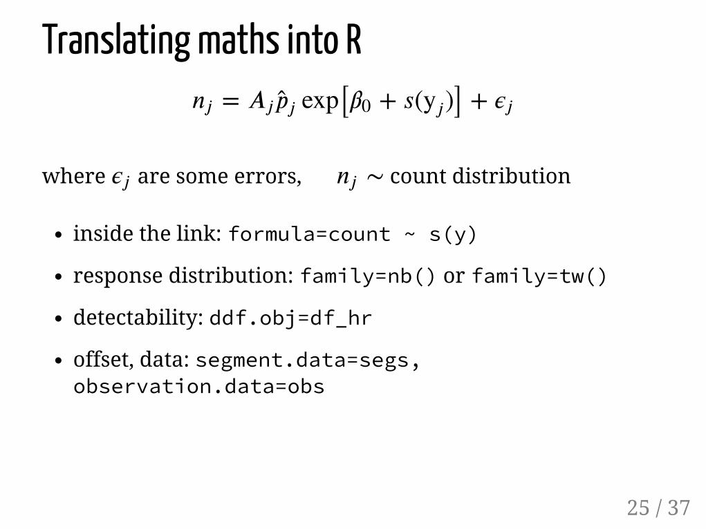
Translating maths into R
where are some errors, count distribution
inside the link: formula=count ~ s(y)
response distribution: family=nb() or family=tw()
detectability: ddf.obj=df_hr
offset, data: segment.data=segs,observation.data=obs
= exp[ + 𝑠( )] +𝑛𝑗 𝐴𝑗 �̂� 𝑗 𝛽0 y𝑗 𝜖𝑗
𝜖𝑗 ∼𝑛𝑗
25 / 37
Your �rst DSMlibrary(dsm)dsm_x_tw <- dsm(count~s(x), ddf.obj=df, segment.data=segs, observation.data=obs, family=tw())
26 / 37
summary(dsm_x_tw)## ## Family: Tweedie(p=1.326) ## Link function: log ## ## Formula:## count ~ s(x) + offset(off.set)## ## Parametric coefficients:## Estimate Std. Error t value Pr(>|t|) ## (Intercept) -19.8115 0.2277 -87.01 <2e-16 ***## ---## Signif. codes: 0 '***' 0.001 '**' 0.01 '*' 0.05 '.' 0.1 ' ' 1## ## Approximate significance of smooth terms:## edf Ref.df F p-value ## s(x) 4.962 6.047 6.403 1.79e-06 ***## ---## Signif. codes: 0 '***' 0.001 '**' 0.01 '*' 0.05 '.' 0.1 ' ' 1## ## R-sq.(adj) = 0.0283 Deviance explained = 17.9%## -REML = 409.94 Scale est. = 6.0413 n = 949
27 / 37
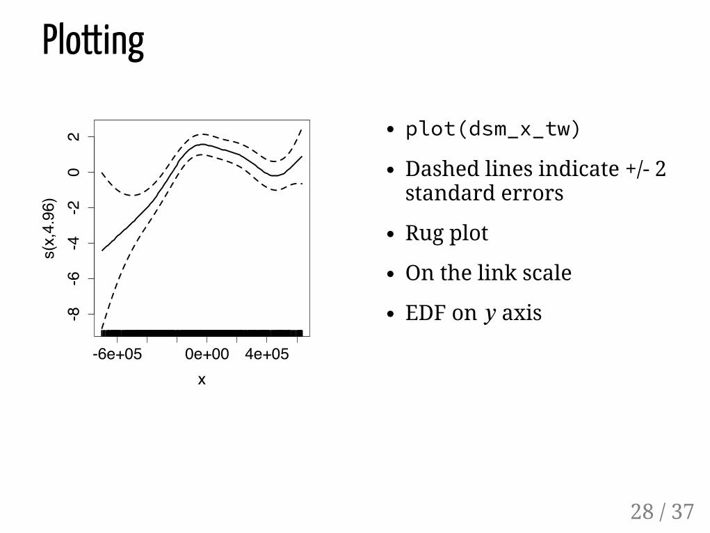
plot(dsm_x_tw)
Dashed lines indicate +/- 2standard errors
Rug plot
On the link scale
EDF on axis
Plotting
𝑦
28 / 37
Adding a termJust use +
dsm_xy_tw <- dsm(count ~ s(x) + s(y), ddf.obj=df, segment.data=segs, observation.data=obs, family=tw())
29 / 37
summary(dsm_xy_tw)## ## Family: Tweedie(p=1.306) ## Link function: log ## ## Formula:## count ~ s(x) + s(y) + offset(off.set)## ## Parametric coefficients:## Estimate Std. Error t value Pr(>|t|) ## (Intercept) -20.0908 0.2381 -84.39 <2e-16 ***## ---## Signif. codes: 0 '***' 0.001 '**' 0.01 '*' 0.05 '.' 0.1 ' ' 1## ## Approximate significance of smooth terms:## edf Ref.df F p-value ## s(x) 4.943 6.057 3.224 0.00425 ** ## s(y) 5.293 6.419 4.034 0.00033 ***## ---## Signif. codes: 0 '***' 0.001 '**' 0.01 '*' 0.05 '.' 0.1 ' ' 1## ## R-sq.(adj) = 0.0678 Deviance explained = 27.4%## -REML = 399.84 Scale est. = 5.3157 n = 949
30 / 37
Plottingplot(dsm_xy_tw, pages=1)
31 / 37
Bivariate termsAssumed an additive structure
No interaction
We can specify s(x,y) (and s(x,y,z,...))
32 / 37
Bivariate spatial termdsm_xyb_tw <- dsm(count ~ s(x, y), ddf.obj=df, segment.data=segs, observation.data=obs, family=tw())
33 / 37
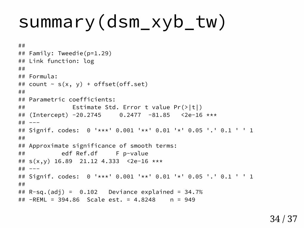
summary(dsm_xyb_tw)## ## Family: Tweedie(p=1.29) ## Link function: log ## ## Formula:## count ~ s(x, y) + offset(off.set)## ## Parametric coefficients:## Estimate Std. Error t value Pr(>|t|) ## (Intercept) -20.2745 0.2477 -81.85 <2e-16 ***## ---## Signif. codes: 0 '***' 0.001 '**' 0.01 '*' 0.05 '.' 0.1 ' ' 1## ## Approximate significance of smooth terms:## edf Ref.df F p-value ## s(x,y) 16.89 21.12 4.333 <2e-16 ***## ---## Signif. codes: 0 '***' 0.001 '**' 0.01 '*' 0.05 '.' 0.1 ' ' 1## ## R-sq.(adj) = 0.102 Deviance explained = 34.7%## -REML = 394.86 Scale est. = 4.8248 n = 949
34 / 37
plot(dsm_xyb_tw, select=1, scheme=2, asp=1)
On link scale
scheme=2 makesheatmap
(set too.far to excludepoints far from data)
Plotting
35 / 37
Comparing bivariate and additive models
36 / 37
Let's have a go...Let's have a go...
37 / 3737 / 37
Lecture 2 : Generalized Additive ModelsLecture 2 : Generalized Additive Models
1 / 371 / 37

OverviewThe count model, from scratch
What is a GAM?
What is smoothing?
Fitting GAMs using dsm
2 / 37

Building a model, from scratchKnow count in segment 𝑛𝑗 𝑗
3 / 37

Building a model, from scratchKnow count in segment
Want :
𝑛𝑗 𝑗
= 𝑓([environmental covariates )𝑛𝑗 ]𝑗
4 / 37

Building a model, from scratchKnow count in segment
Want :
How to build ?
𝑛𝑗 𝑗
= 𝑓([environmental covariates )𝑛𝑗 ]𝑗
𝑓
5 / 37

Building a model, from scratchKnow count in segment
Want :
How to build ?
Additive model of smooths :
is the link function
𝑛𝑗 𝑗
= 𝑓([environmental covariates )𝑛𝑗 ]𝑗
𝑓
𝑠
= exp [ + 𝑠( ) + 𝑠( )]𝑛𝑗 𝛽0 y𝑗 Depth𝑗
model terms
exp
6 / 37

Building a model, from scratch
What about area and detectability?
area of segment - "offset"
probability of detection in segment
= exp [ + 𝑠( ) + 𝑠( )]𝑛𝑗 𝐴𝑗 �̂� 𝑗 𝛽0 y𝑗 Depth𝑗
𝐴𝑗
�̂� 𝑗
7 / 37
Building a model, from scratch
It's a statistical model so:
has a distribution (count)
are residuals (differences between model andobservations)
= exp [ + 𝑠( ) + 𝑠( )] +𝑛𝑗 𝐴𝑗 �̂� 𝑗 𝛽0 y𝑗 Depth𝑗 𝜖𝑗
𝑛𝑗
𝜖𝑗
8 / 37

That's a Generalized Additive Model!That's a Generalized Additive Model!
9 / 379 / 37

Now let's look at each bit...Now let's look at each bit...
10 / 3710 / 37

Response
where
= exp[ + 𝑠( ) + 𝑠( )] +𝑛𝑗 𝐴𝑗 �̂� 𝑗 𝛽0 y𝑗 Depth𝑗 𝜖𝑗
∼ count distribution𝑛𝑗
11 / 37

Response is a count
Often, it's mostly zero
mean variance
(Poisson isn't good atthis)
Count distributions
≠
12 / 37

(NB there is a point mass atzero not plotted)
Poisson is
We estimate:
(p in R), "power"parameter
(Scale est. in R),scale parameter
Tweedie distribution
Var (count) = 𝜙𝔼(count)𝑞
𝑞 = 1
𝑞
𝜙
13 / 37

Estimate
No scale parameter(Scale est.=1 always)
(Poisson: )
Negative binomial distribution
Var (count) =
𝔼(count) + 𝜅𝔼(count)2
𝜅
Var (count) = 𝔼(count)
14 / 37

Smooths= exp[ + 𝑠( ) + 𝑠( )] +𝑛𝑗 𝐴𝑗 �̂� 𝑗 𝛽0 y𝑗 Depth𝑗 𝜖𝑗
15 / 37

Think =smooth
Want a line that is "close"to all the data
Balance betweeninterpolation and "fit"
What about these "s" things?
𝑠
16 / 37

What is smoothing?What is smoothing?
17 / 3717 / 37

SmoothingWe think underlying phenomenon is smooth
"Abundance is a smooth function of depth"
1, 2 or more dimensions
18 / 37

We set:
"type": bases (made upof basis functions)
"maximumwigglyness": basis size(sometimes:dimension/complexity)
Automatically estimate:
"how wiggly it needsto be": smoothingparameter(s)
Estimating smooths
19 / 37

SplinesFunctions made of other, simpler functions
Basis functions , estimate 𝑏𝑘 𝛽𝑘
𝑠(𝑥) = (𝑥)∑𝐾
𝑘=1𝛽𝑘𝑏𝑘
20 / 37

Thinking about wigglynessVisually:
Lots of wiggles not smooth
Straight line very smooth
Smoothing parameter ( ) controls this
⇒
⇒
𝜆
21 / 37

How wiggly are things?Measure the effective degrees of freedom (EDF)
Set basis complexity or "size",
Set "large enough"
𝑘
𝑘
22 / 37

I can't teach you all ofGAMs in 1 week
Good intro book
(also a good textbook onGLMs and GLMMs)
Quite technical in places
More resources on coursewebsite
dsm is based on mgcv bySimon Wood
Getting more out of GAMs
23 / 37

Fitting GAMs using dsmFitting GAMs using dsm
24 / 3724 / 37
Translating maths into R
where are some errors, count distribution
inside the link: formula=count ~ s(y)
response distribution: family=nb() or family=tw()
detectability: ddf.obj=df_hr
offset, data: segment.data=segs,observation.data=obs
= exp[ + 𝑠( )] +𝑛𝑗 𝐴𝑗 �̂� 𝑗 𝛽0 y𝑗 𝜖𝑗
𝜖𝑗 ∼𝑛𝑗
25 / 37

Your �rst DSMlibrary(dsm)dsm_x_tw <- dsm(count~s(x), ddf.obj=df, segment.data=segs, observation.data=obs, family=tw())
26 / 37

summary(dsm_x_tw)## ## Family: Tweedie(p=1.326) ## Link function: log ## ## Formula:## count ~ s(x) + offset(off.set)## ## Parametric coefficients:## Estimate Std. Error t value Pr(>|t|) ## (Intercept) -19.8115 0.2277 -87.01 <2e-16 ***## ---## Signif. codes: 0 '***' 0.001 '**' 0.01 '*' 0.05 '.' 0.1 ' ' 1## ## Approximate significance of smooth terms:## edf Ref.df F p-value ## s(x) 4.962 6.047 6.403 1.79e-06 ***## ---## Signif. codes: 0 '***' 0.001 '**' 0.01 '*' 0.05 '.' 0.1 ' ' 1## ## R-sq.(adj) = 0.0283 Deviance explained = 17.9%## -REML = 409.94 Scale est. = 6.0413 n = 949
27 / 37
plot(dsm_x_tw)
Dashed lines indicate +/- 2standard errors
Rug plot
On the link scale
EDF on axis
Plotting
𝑦
28 / 37

Adding a termJust use +
dsm_xy_tw <- dsm(count ~ s(x) + s(y), ddf.obj=df, segment.data=segs, observation.data=obs, family=tw())
29 / 37

summary(dsm_xy_tw)## ## Family: Tweedie(p=1.306) ## Link function: log ## ## Formula:## count ~ s(x) + s(y) + offset(off.set)## ## Parametric coefficients:## Estimate Std. Error t value Pr(>|t|) ## (Intercept) -20.0908 0.2381 -84.39 <2e-16 ***## ---## Signif. codes: 0 '***' 0.001 '**' 0.01 '*' 0.05 '.' 0.1 ' ' 1## ## Approximate significance of smooth terms:## edf Ref.df F p-value ## s(x) 4.943 6.057 3.224 0.00425 ** ## s(y) 5.293 6.419 4.034 0.00033 ***## ---## Signif. codes: 0 '***' 0.001 '**' 0.01 '*' 0.05 '.' 0.1 ' ' 1## ## R-sq.(adj) = 0.0678 Deviance explained = 27.4%## -REML = 399.84 Scale est. = 5.3157 n = 949
30 / 37

Plottingplot(dsm_xy_tw, pages=1)
31 / 37

Bivariate termsAssumed an additive structure
No interaction
We can specify s(x,y) (and s(x,y,z,...))
32 / 37

Bivariate spatial termdsm_xyb_tw <- dsm(count ~ s(x, y), ddf.obj=df, segment.data=segs, observation.data=obs, family=tw())
33 / 37
summary(dsm_xyb_tw)## ## Family: Tweedie(p=1.29) ## Link function: log ## ## Formula:## count ~ s(x, y) + offset(off.set)## ## Parametric coefficients:## Estimate Std. Error t value Pr(>|t|) ## (Intercept) -20.2745 0.2477 -81.85 <2e-16 ***## ---## Signif. codes: 0 '***' 0.001 '**' 0.01 '*' 0.05 '.' 0.1 ' ' 1## ## Approximate significance of smooth terms:## edf Ref.df F p-value ## s(x,y) 16.89 21.12 4.333 <2e-16 ***## ---## Signif. codes: 0 '***' 0.001 '**' 0.01 '*' 0.05 '.' 0.1 ' ' 1## ## R-sq.(adj) = 0.102 Deviance explained = 34.7%## -REML = 394.86 Scale est. = 4.8248 n = 949
34 / 37

plot(dsm_xyb_tw, select=1, scheme=2, asp=1)
On link scale
scheme=2 makesheatmap
(set too.far to excludepoints far from data)
Plotting
35 / 37

Comparing bivariate and additive models
36 / 37

Let's have a go...Let's have a go...
37 / 3737 / 37
Related Documents


