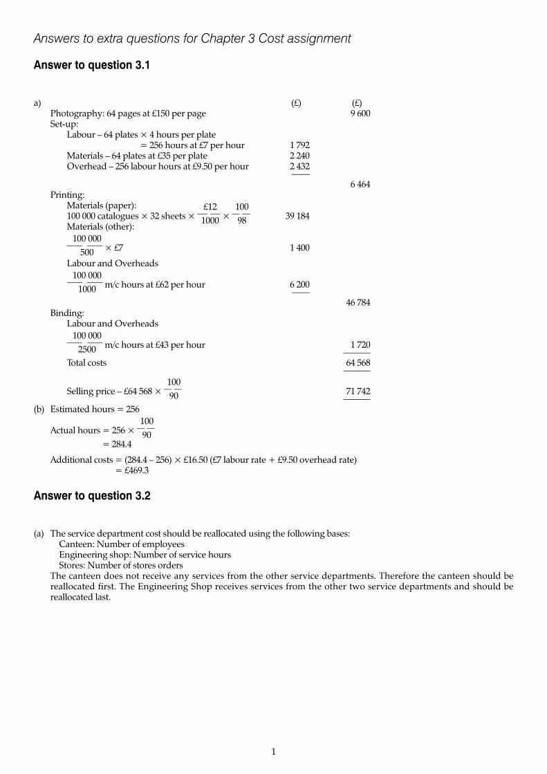
Answers to extra questions for Chapter 3 Cost assignment Answer to question 3.1 a) (£) (£) Photography: 64 pages at £150 per page 9 600 Set-up: Labour – 64 plates × 4 hours per plate = 256 hours at £7 per hour 1 792 Materials – 64 plates at £35 per plate 2 240 Overhead – 256 labour hours at £9.50 per hour 2 432 –––– 6 464 Printing: Materials (paper): 100 000 catalogues × 32 sheets × 1 £ 0 1 0 2 0 × 1 9 0 8 0 39 184 Materials (other): 10 5 0 0 0 0 00 × £7 1 400 Labour and Overheads 10 1 0 00 0 0 00 m/c hours at £62 per hour 6 200 –––– 46 784 Binding: Labour and Overheads 10 2 0 50 0 0 00 m/c hours at £43 per hour 1 720 –––––– Total costs 64 568 –––––– Selling price – £64 568 × 1 9 0 0 0 71 742 –––––– (b) Estimated hours = 256 Actual hours = 256 × 1 9 0 0 0 = 284.4 Additional costs = (284.4 – 256) × £16.50 (£7 labour rate + £9.50 overhead rate) = £469.3 Answer to question 3.2 (a) The service department cost should be reallocated using the following bases: Canteen: Number of employees Engineering shop: Number of service hours Stores: Number of stores orders The canteen does not receive any services from the other service departments. Therefore the canteen should be reallocated first. The Engineering Shop receives services from the other two service departments and should be reallocated last. 1

Welcome message from author
This document is posted to help you gain knowledge. Please leave a comment to let me know what you think about it! Share it to your friends and learn new things together.
Transcript
Answers to extra questions for Chapter 3 Cost assignment
Answer to question 3.1
a) (£) (£)Photography: 64 pages at £150 per page 9 600Set-up:
Labour – 64 plates × 4 hours per plate= 256 hours at £7 per hour 1 792
Materials – 64 plates at £35 per plate 2 240Overhead – 256 labour hours at £9.50 per hour 2 432
––––6 464
Printing:Materials (paper):100 000 catalogues × 32 sheets × �1
£01020
� × �19080
� 39 184Materials (other):
�10
5000000
� × £7 1 400
Labour and Overheads
�10
1000
0000
� m/c hours at £62 per hour 6 200––––
46 784Binding:
Labour and Overheads
�10
2050
0000
� m/c hours at £43 per hour 1 720––––––
Total costs 64 568––––––
Selling price – £64 568 × �19000
� 71 742––––––
(b) Estimated hours = 256
Actual hours = 256 × �19000
�
= 284.4
Additional costs = (284.4 – 256) × £16.50 (£7 labour rate + £9.50 overhead rate)= £469.3
Answer to question 3.2
(a) The service department cost should be reallocated using the following bases:Canteen: Number of employeesEngineering shop: Number of service hoursStores: Number of stores orders
The canteen does not receive any services from the other service departments. Therefore the canteen should bereallocated first. The Engineering Shop receives services from the other two service departments and should bereallocated last.
1
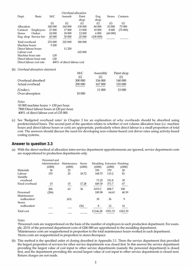
Overhead allocationDept. Basis M/C Assemb Paint Eng Stores Canteen
shop shop(£) (£) (£) (£) (£) (£)
Allocation 180 000 160 000 130 000 84 000 52 000 75 000Canteen Employees 27 000 17 000 13 000 10 000 8 000 (75 000)Stores Orders 24 000 18 000 12 000 6 000 (60 000)Eng. shop Service hrs 45 000 30 000 25 000 (100 000)
–––––– –––––– –––––– ––––––– –––––– ––––––Total overhead 276 000 225 000 180 000Machine hours 9 200Direct labour hours 11 250Labour cost £45 000Machine hour rate £30Direct labour hour rate £20Direct labour cost rate 400% of direct labour cost
(b) Overhead absorption statementM/C Assembly Paint shop(£) (£) (£)
Overhead absorbeda 300 000 156 000 140 000Actual overhead 290 000 167 000 155 000–––––– –––––– ––––––(Under-) 11 000 15 000Over-absorption 10 000
Notesa10 000 machine hours � £30 per hour.a7800 Direct labour hours at £20 per hour.a400% of direct labour cost of £35 000.
(c) See ‘Budgeted overhead rates’ in Chapter 3 for an explanation of why overheads should be absorbed usingpredetermined bases. The second part of the question relates to whether or not volume allocation base (i.e. machinehours and direct labour hours or cost) are appropriate, particularly when direct labour is a small proportion of totalcost. The answers should discuss the need for developing non-volume-based cost driver rates using activity-basedcosting systems.
Answer to question 3.3(a) With the direct method of allocation inter-service department apportionments are ignored, service department costs
are reapportioned to production departments only.
Personnel andAdministration Maintenance Stores Moulding Extrusion Finishing
(£000) (£000) (£000) (£000) (£000) (£000)Materials 36 23 330 170 20Labour 155 25 18.72 168.75 115.2 81Variable
overhead 71.25 151.8 30Fixed overhead 15 15 17.28 449.30 371.7 67
––– ––– ––––– –––––– ––––– ––––206 63 36 1019.3 808.7 198
Personnela (206) 100.98 64.63 40.39Maintenance
reallocationb (63) 18 36 9Stores
reallocationc (36) 8 12 16––– ––– ––––– –––––– ––––– ––––
Total cost £1146.28 £921.33 £263.39––– ––– ––––– –––––– ––––– ––––
NotesaPersonnel costs are reapportioned on the basis of the number of employees in each production department. For exam-ple, 25/51 of the personnel department costs of £206 000 are apportioned to the moulding department.bMaintenance costs are reapportioned in proportion to the total maintenance hours worked in each department.cStores costs are reapportioned in proportion to stores floorspace.
(b) This method is the specified order of closing described in Appendix 3.1. There the service department that providedthe largest proportion of services for other service departments was closed first. In this answer the service departmentproviding the largest value of cost input to other service departments (namely the personnel department) is closedfirst, and the department providing the second largest value of cost input to other service departments is closed next.Return charges are not made.
2
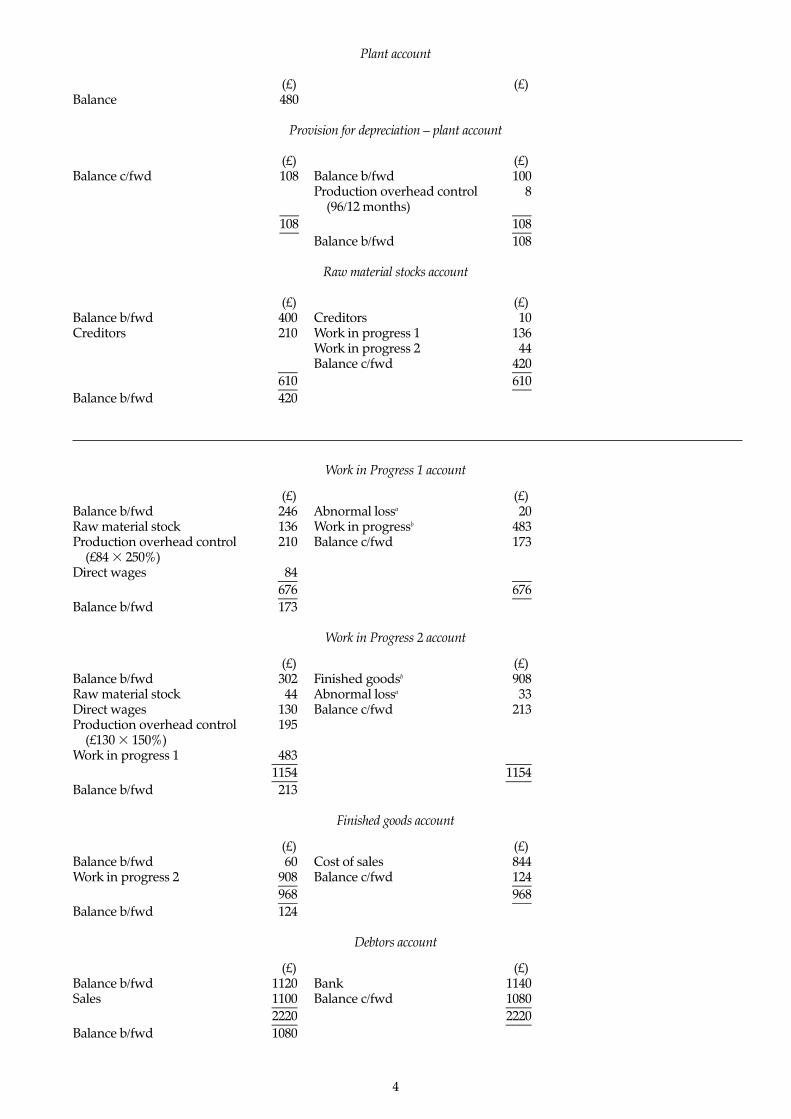
Personnel andAdministration Maintenance Stores Moulding Extrusion Finishing
(£000) (£000) (£000) (£000) (£000) (£000)Original
allocation 206 63 36 1019.3 808.7 198Personnel
reallocation (206) 14.21(4/58) 10.65(3/58) 88.79(25/58) 56.83(16/58) 35.52(10/58)–––––––––
Maintenancereallocation (77.21) 13.63(15/85) 18.17(20/85) 36.33(40/85) 9.08(10/85)
––––––––––Stores
reallocation (60.28) 13.4(20/90) 20.09(30/90) 26.79(40/90)
Total cost £1139.66 £921.95 £269.39
(c) The reciprocal method incorporates all inter-servicing relationships. Let
P � total cost of personnel and administrationM � total cost of maintenanceS � total cost of stores
The total costs that will be transferred to the service departments can be expressed as:
P � 206 � 0.0556M (W1)M � 63 � 0.0690P (W2) � 0.15 (W3)S � 36 � 0.166M (W4) � 0.0517P (W5)
The total costs of the production department will be:
Moulding (£000) 1019.3 � 0.431P (W6) � 0.22M (W7) � 0.2S (W8)Extrusion (£000) 808.7 � 0.276P (W9) � 0.44M (W10) � 0.3S (W11)Finishing (£000) 198.0 � 0.172P (W12) � 0.11M (W13) � 0.4S (W14)
Workings(W1) M coefficient � 5/90 (W8) S coefficient � 20/100(W2) P coefficient � 4/58 (W9) P coefficient � 16/58(W3) S coefficient � 10/100 (W10) P coefficient � 40/90(W4) M coefficient � 15/90 (W11) S coefficient � 30/100(W5) P coefficient � 3/58 (W12) P coefficient � 10/58(W6) P coefficient � 25/58 (W13) M coefficient � 10/90(W7) M coefficient � 20/90 (W14) S coefficient � 40/100
(d) The direct method is the simplest, but ignores inter-service department apportionments. If there is a significant pro-portion of inter-servicing apportionments, this method is likely to result in inaccurate calculations.
The step-down method gives partial recognition to inter-department servicing, and does not involve time-consuming apportionments. The reciprocal method takes full account of inter-department servicing, and is the onlymethod that will yield accurate results.
The choice of method will depend on cost behaviour. If a significant proportion of costs are variable then servicedepartment reallocations will be important for decision-making and cost control. In this situation the reciprocalmethod should be used. However, if the vast majority of costs are fixed, the cost allocations should not be used for costcontrol and decision-making, and here is a case for using the direct or step-down method.
(e) The answer to this question should include a discussion of cost-plus pricing. See ‘Limitations of cost-plus pricing’ and‘Reasons for using cost-plus pricing’ in Chapter 11 for the answer to this question.
Answers to extra questions for Chapter 4 Accounting entries for a job costing system
Answer to question 4.1
(a) The opening WIP balance indicates that overheads are absorbed as follows:
Process 1 � Production overhead (125)/Direct wages (50) � 250% of direct wagesProcess 2 � Production overhead (105)/Direct wages (70) � 150% of direct wages
(b) NB Limited accounts (All figures in £000)
Building account
(£) (£)Balance 800
3
Plant account
(£) (£)Balance 480
Provision for depreciation – plant account
(£) (£)Balance c/fwd 108 Balance b/fwd 100
Production overhead control 8(96/12 months)––– –––
108 108––– –––Balance b/fwd 108
Raw material stocks account
(£) (£)Balance b/fwd 400 Creditors 10Creditors 210 Work in progress 1 136
Work in progress 2 44Balance c/fwd 420––– –––
610 610––– –––Balance b/fwd 420
Work in Progress 1 account
(£) (£)Balance b/fwd 246 Abnormal lossa 20Raw material stock 136 Work in progressb 483Production overhead control 210 Balance c/fwd 173
(£84 � 250%)Direct wages 84––– –––
676 676––– –––Balance b/fwd 173
Work in Progress 2 account
(£) (£)Balance b/fwd 302 Finished goodsb 908Raw material stock 44 Abnormal lossa 33Direct wages 130 Balance c/fwd 213Production overhead control 195
(£130 � 150%)Work in progress 1 483–––– ––––
1154 1154–––– ––––Balance b/fwd 213
Finished goods account
(£) (£)Balance b/fwd 60 Cost of sales 844Work in progress 2 908 Balance c/fwd 124––– –––
968 968––– –––Balance b/fwd 124
Debtors account
(£) (£)Balance b/fwd 1120 Bank 1140Sales 1100 Balance c/fwd 1080–––– ––––
2220 2220–––– ––––Balance b/fwd 1080
4
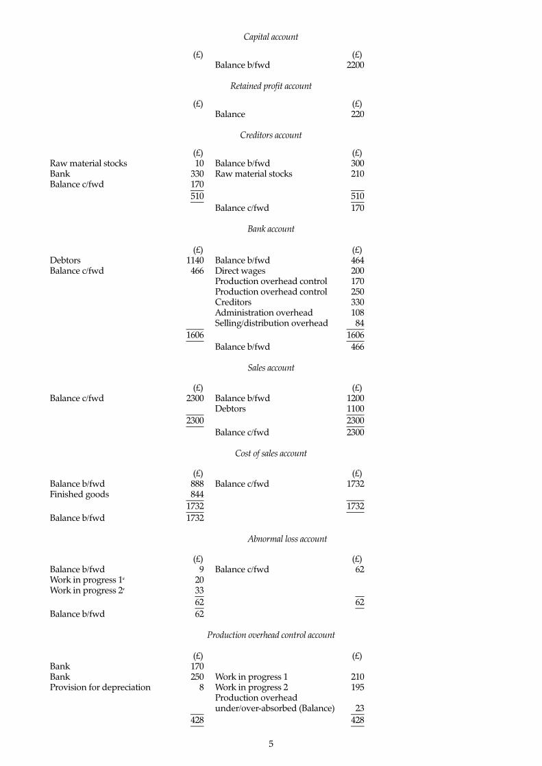
Capital account
(£) (£)Balance b/fwd 2200
Retained profit account
(£) (£)Balance 220
Creditors account
(£) (£)Raw material stocks 10 Balance b/fwd 300Bank 330 Raw material stocks 210Balance c/fwd 170––– –––
510 510––– –––Balance c/fwd 170
Bank account
(£) (£)Debtors 1140 Balance b/fwd 464Balance c/fwd 466 Direct wages 200
Production overhead control 170Production overhead control 250Creditors 330Administration overhead 108Selling/distribution overhead 84–––– ––––
1606 1606–––– ––––Balance b/fwd 466
Sales account
(£) (£)Balance c/fwd 2300 Balance b/fwd 1200
Debtors 1100–––– ––––2300 2300–––– ––––
Balance c/fwd 2300
Cost of sales account
(£) (£)Balance b/fwd 888 Balance c/fwd 1732Finished goods 844–––– ––––
1732 1732–––– ––––Balance b/fwd 1732
Abnormal loss account
(£) (£)Balance b/fwd 9 Balance c/fwd 62Work in progress 1a 20Work in progress 2a 33–– ––
62 62–– ––Balance b/fwd 62
Production overhead control account
(£) (£)Bank 170Bank 250 Work in progress 1 210Provision for depreciation 8 Work in progress 2 195
Production overheadunder/over-absorbed (Balance) 23––– –––
428 428––– –––
5
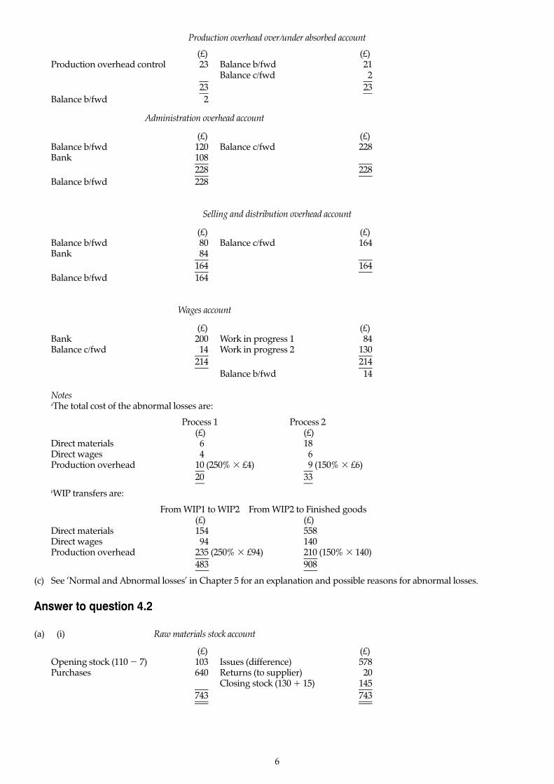
Production overhead over/under absorbed account
(£) (£)Production overhead control 23 Balance b/fwd 21
Balance c/fwd 2–– ––23 23–– ––
Balance b/fwd 2
Administration overhead account
(£) (£)Balance b/fwd 120 Balance c/fwd 228Bank 108––– –––
228 228––– –––Balance b/fwd 228
Selling and distribution overhead account
(£) (£)Balance b/fwd 80 Balance c/fwd 164Bank 84––– –––
164 164––– –––Balance b/fwd 164
Wages account
(£) (£)Bank 200 Work in progress 1 84Balance c/fwd 14 Work in progress 2 130––– –––
214 214––– –––Balance b/fwd 14
NotesaThe total cost of the abnormal losses are:
Process 1 Process 2(£) (£)
Direct materials 6 18Direct wages 4 6Production overhead 10 (250% � £4) 9 (150% � £6)–– ––
20 33–– ––bWIP transfers are:
From WIP1 to WIP2 From WIP2 to Finished goods(£) (£)
Direct materials 154 558Direct wages 94 140Production overhead 235 (250% � £94) 210 (150% � 140)––– –––
483 908––– –––(c) See ‘Normal and Abnormal losses’ in Chapter 5 for an explanation and possible reasons for abnormal losses.
Answer to question 4.2
(a) (i) Raw materials stock account
(£) (£)Opening stock (110 � 7) 103 Issues (difference) 578Purchases 640 Returns (to supplier) 20
Closing stock (130 � 15) 145––– –––743 743––– –––––– –––
6
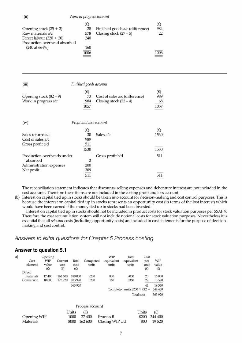
(ii) Work in progress account
(£) (£)Opening stock (25 � 3) 28 Finished goods a/c (difference) 984Raw materials a/c 578 Closing stock (27 – 5) 22Direct labour (220 � 20) 240Production overhead absorbed
(240 at 66 ��%) 160–––– ––––1006 1006–––– –––––––– ––––
(iii) Finished goods account
(£) (£)Opening stock (82 – 9) 73 Cost of sales a/c (difference) 989Work in progress a/c 984 Closing stock (72 – 4) 68–––– ––––
1057 1057–––– –––––––– ––––
(iv) Profit and loss account
(£) (£)Sales returns a/c 30 Sales a/c 1530Cost of sales a/c 989Gross profit c/d 511–––– ––––
1530 1530–––– –––––––– ––––Production overheads under Gross profit b/d 511
absorbed 2Administration expenses 200Net profit 309––– –––
511 511––– –––––– –––
The reconciliation statement indicates that discounts, selling expenses and debenture interest are not included in thecost accounts. Therefore these items are not included in the costing profit and loss account.
(b) Interest on capital tied up in stocks should be taken into account for decision-making and cost control purposes. This isbecause the interest on capital tied up in stocks represents an opportunity cost (in terms of the lost interest) whichwould have been earned if the money tied up in stocks had been invested.
Interest on capital tied up in stocks should not be included in product costs for stock valuation purposes per SSAP 9.Therefore the cost accumulation system will not include notional costs for stock valuation purposes. Nevertheless it isessential that all relevant costs (including opportunity costs) are included in cost statements for the purpose of decision-making and cost control.
Answers to extra questions for Chapter 5 Process costing
Answer to question 5.1a) Opening WIP Total Cost
Cost WIP Current Total Completed equivalent equivalent per WIPelement value cost cost units units units unit value
(£) (£) (£) (£) (£)Direct
materials 17 400 162 600 180 000 8200 800 9000 20 16 000Conversion 10 000 173 920 183 920 8200 160 8360 22 3 520–––––– ––––––––––
363 920 42 19 520Completed units 8200 � £42 � 344 400––––––
Total cost 363 920––––––
Process accountUnits (£) Units (£)
Opening WIP 1000 27 400 Process B 8200 344 400Materials 8000 162 600 Closing WIP c/d 800 19 520
7
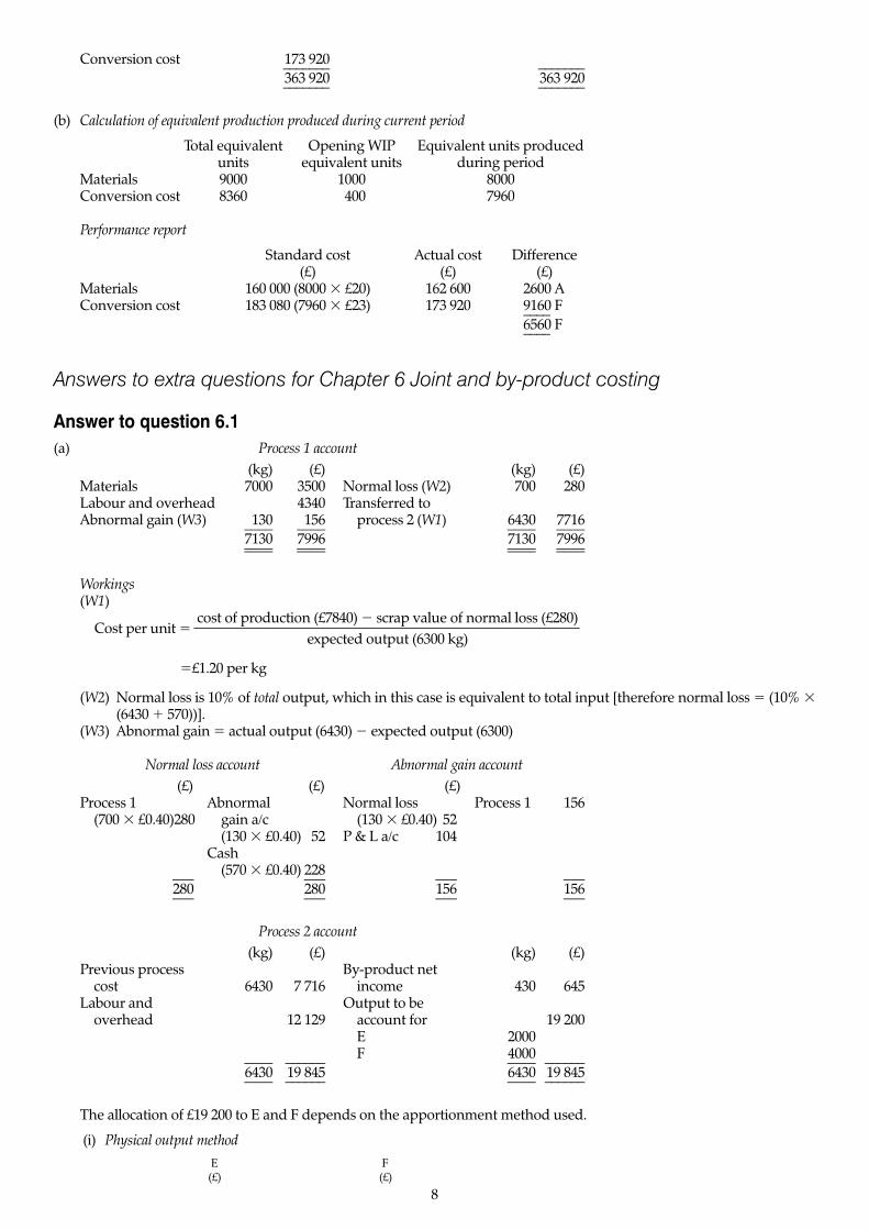
Conversion cost 173 920––––––– –––––––363 920 363 920––––––– –––––––
(b) Calculation of equivalent production produced during current period
Total equivalent Opening WIP Equivalent units producedunits equivalent units during period
Materials 9000 1000 8000Conversion cost 8360 400 7960
Performance report
Standard cost Actual cost Difference(£) (£) (£)
Materials 160 000 (8000 � £20) 162 600 2600 A Conversion cost 183 080 (7960 � £23) 173 920 9160 F––––
6560 F––––
Answers to extra questions for Chapter 6 Joint and by-product costing
Answer to question 6.1(a) Process 1 account
(kg) (£) (kg) (£)Materials 7000 3500 Normal loss (W2) 700 280Labour and overhead 4340 Transferred toAbnormal gain (W3) 130 156 process 2 (W1) 6430 7716–––– –––– –––– ––––
7130 7996 7130 7996–––– –––– –––– –––––––– –––– –––– ––––
Workings(W1)
Cost per unit �cost of production (£7840) � scrap value of normal loss (£280)
expected output (6300 kg)
�£1.20 per kg
(W2) Normal loss is 10% of total output, which in this case is equivalent to total input [therefore normal loss � (10% �(6430 � 570))].
(W3) Abnormal gain � actual output (6430) � expected output (6300)
Normal loss account Abnormal gain account(£) (£) (£)
Process 1 Abnormal Normal loss Process 1 156(700 � £0.40)280 gain a/c (130 � £0.40) 52
(130 � £0.40) 52 P & L a/c 104Cash
(570 � £0.40) 228––– ––– ––– –––280 280 156 156––– ––– ––– –––
Process 2 account(kg) (£) (kg) (£)
Previous process By-product netcost 6430 7 716 income 430 645
Labour and Output to beoverhead 12 129 account for 19 200
E 2000F 4000–––– –––––– –––– ––––––
6430 19 845 6430 19 845–––– –––––– –––– ––––––
The allocation of £19 200 to E and F depends on the apportionment method used.
(i) Physical output methodE F(£) (£)
8
1. Total output cost 6400 �2000� £19 200� 12 800 �4000
� £19 200�6000 6000
2. Closing stock 2880 �2000 � 1100 � £6400� 2 560 �4000 � 3200
� £12 800�2000 4000
3. Cost of sales 3520 �1100� £6400� 10 240 �3200
� £12 800�2000 4000
4. Sales revenue 7700 (1100 � £7) 8 000 (3200 � £2.50)
5. Profit (4 � 3) 4180 (2 240)
(ii) Market value of output methodE F
(£) (£)
1. Market value of output 14 000 (2000 � £7) 10 000 (4000 � £2.50)
2. Cost of output 11 200 ��1244� � £19 200� 8 000 ��
1204� � £19 200�
3. Closing stock 5 040 ��[2900000]
� � £11 200� 1 600 ��[4800000]
� � £8 000�4. Cost of sales 6 160 ��
12100000
� � £11 200� 6 400 ��34200000
� � £8 000�5. Sales revenue 7 700 8 000
6. Profit (5 � 4) 1 540 1 600
(c) See Chapter 6 for the answer to this question. In particular, the answer should stress that joint cost apportionments arenecessary for stock valuation, but such apportionments are inappropriate for decision-making. For decision-makingrelevant costs should be used. It can be seen from the answer to part (b) that one method of apportionment impliesthat F makes a loss whereas the other indicates that F makes a profit. Product F should only be deleted if the costssaved from deleting it exceed the revenues lost.
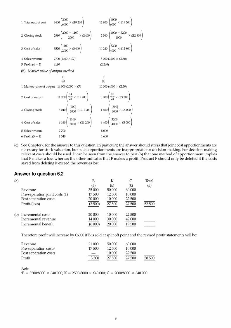
Answer to question 6.2(a) B K C Total
(£) (£) (£) (£)Revenue 35 000 50 000 60 000Pre-separation joint costs (1) 17 500 12 500 10 000Post separation costs 20 000 10 000 22 500–––––– –––––– –––––– ––––––Profit/(loss) (2 500) 27 500 27 500 52 500–––––– –––––– –––––– ––––––
(b) Incremental costs 20 000 10 000 22 500Incremental revenue 14 000 30 000 42 000–––––– –––––– –––––– ––––––Incremental benefit (6 000) 20 000 19 500–––––– –––––– –––––– ––––––
Therefore profit will increase by £6000 if B is sold at split off point and the revised profit statements will be:
Revenue 21 000 50 000 60 000Pre-separation costsa 17 500 12 500 10 000Post separation costs — 10 000 22 500–––––– –––––– –––––– ––––––Profit 3 500 27 500 27 500 58 500–––––– –––––– –––––– ––––––
NoteaB � 3500/8000 � £40 000; K � 2500/8000 � £40 000; C � 2000/8000 � £40 000.
9

Answers to extra questions for Chapter 7 Income effects of alternative costaccumulation systems
Answer to question 7.1(a) See sections on some arguments in support of variable costing and some arguments in support of absorption costing in
Chapter 7 for the answer to this question.(b) (i) (£)
Fixed production overhead per unit = 0.60 (£144 000/240 000 units)Variable production cost per unit = 1.30 (£312 000/240 000 units)Variable selling and administration
overhead per unit = 0.10 (£24 000/240 000 units)Fixed selling and administration
overhead per unit = 0.40 (£96 000/240 000 units)–––2.40
Selling price 3.00–––Profit 0.60–––
(£)Fixed production overhead incurred 144 000 Fixed production overhead absorbed (260 000 � £0.60) 156 000–––––––Over-recovery £12 000–––––––
(ii) Absorption costing profit:(£)
Opening stock (40 000 � £1.90) 76 000Production cost (260 000 � £1.90) 494 000–––––––
570 000Less closing stock (70 000 � £1.90) 133 000–––––––Cost of sales (230 000 � £1.90) 437 000Less over recovery of fixed production overhead 12 000–––––––
425 000
Selling and administration overhead:Variable (230 000 � £0.10) 23 000
Fixed 96 000–––––––Total cost 544 000Sales (230 000 � £3) 690 000––––––––Profit £146 000––––––––
Marginal costing profit:(£)
Contribution (230 000 � (£3 � £1.40)) 368 000Less fixed costs (£144 000 � £96 000) 240 000––––––––Profit £128 000––––––––
(iii) (£)Absorption costing profit 146 000Fixed overhead included in stock increase (30 000 � £0.60) 18 000––––––––Marginal costing profit £128 000––––––––
(iv) The profit figure will be the same with both systems whenever production equals sales and therefore openingstock equals closing stock.
10
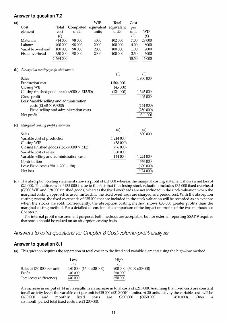
Answer to question 7.2(a) WIP Total Cost
Cost Total Completed equivalent equivalent perelement cost units units units unit WIP
(£) (£) (£)Materials 714 000 98 000 4000 102 000 7.00 28 000Labour 400 000 98 000 2000 100 000 4.00 8000Variable overhead 100 000 98 000 2000 100 000 1.00 2000Fixed overhead 350 000 98 000 2000 100 000 3.50 7000–––––––– ––––– –––––
1 564 000 15.50 45 000–––––––– ––––– –––––
(b) Absorption costing profit statement:(£) (£)
Sales 1 800 000Production cost 1 564 000Closing WIP (45 000)Closing finished goods stock (8000 � £15.50) (124 000) 1 395 000––––––––– –––––––––Gross profit 405 000Less: Variable selling and administrationLess: costs (£1.60 � 90 000) (144 000)Less: Fixed selling and administration costs (250 000)–––––––––Net profit £11 000–––––––––
(c) Marginal costing profit statement:(£) (£)
Sales 1 800 000Variable cost of production 1 214 000Closing WIP (38 000)Closing finished goods stock (8000 � £12) (96 000)–––––––––Variable cost of sales 1 080 000Variable selling and administration costs 144 000 1 224 000––––––––– –––––––––Contribution 576 000Less: Fixed costs (350 � 200 � 50) (600 000)–––––––––Net loss £(24 000)–––––––––
(d) The absorption costing statement shows a profit of £11 000 whereas the marginal costing statement shows a net loss of£24 000. The difference of £35 000 is due to the fact that the closing stock valuation includes £35 000 fixed overhead(£7000 WIP and £28 000 finished goods) whereas the fixed overheads are not included in the stock valuation when themarginal costing approach is used. Instead, all the fixed overheads are charged as a period cost. With the absorptioncosting system, the fixed overheads of £35 000 that are included in the stock valuation will be recorded as an expensewhen the stocks are sold. Consequently, the absorption costing method shows £35 000 greater profits than themarginal costing method. For a detailed discussion of a comparison of the impact on profits of the two methods seeChapter 7.
For internal profit measurement purposes both methods are acceptable, but for external reporting SSAP 9 requiresthat stocks should be valued on an absorption costing basis.
Answers to extra questions for Chapter 8 Cost-volume-profit-analysis
Answer to question 8.1(a) This question requires the separation of total cost into the fixed and variable elements using the high–low method.
Low High(£) (£)
Sales at £30 000 per unit 480 000 (16 � £30 000) 900 000 (30 � £30 000)Profit 40 000 250 000–––––– ––––––Total costs (difference) 440 000 650 000–––––– ––––––
An increase in output of 14 units results in an increase in total costs of £210 000. Assuming that fixed costs are constantfor all activity levels the variable cost per unit is £15 000 (£210 000/14 units). At 30 units activity the variable costs will be£450 000 and monthly fixed costs are £200 000 (£650 000 � £450 000). Over a six-month period total fixed costs are £1 200 000.
11
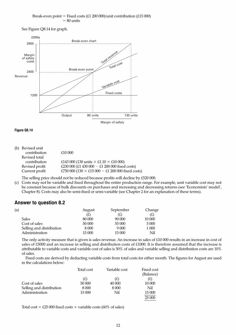
Break-even point � Fixed costs (£1 200 000)/unit contribution (£15 000)� 80 units
See Figure Q8.14 for graph.
(b) Revised unitcontribution £10 000
Revised totalcontribution £143 000 (130 units � £1.10 � £10 000)
Revised profit £230 000 (£1 430 000 � £1 200 000 fixed costs)Current profit £750 000 (130 � £15 000 � £1 200 000 fixed costs)
The selling price should not be reduced because profits will decline by £520 000.(c) Costs may not be variable and fixed throughout the entire production range. For example, unit variable cost may not
be constant because of bulk discounts on purchases and increasing and decreasing returns (see ‘Economists’ model’,Chapter 8). Costs may also be semi-fixed or semi-variable (see Chapter 2 for an explanation of these terms).
Answer to question 8.2(a) August September Change
(£) (£) (£)Sales 80 000 90 000 10 000Cost of sales 50 000 55 000 5 000Selling and distribution 8 000 9 000 1 000Administration 15 000 15 000 Nil
The only activity measure that is given is sales revenue. An increase in sales of £10 000 results in an increase in cost ofsales of £5000 and an increase in selling and distribution costs of £1000. It is therefore assumed that the increase isattributable to variable costs and variable cost of sales is 50% of sales and variable selling and distribution costs are 10%of sales.
Fixed costs are derived by deducting variable costs from total costs for either month. The figures for August are usedin the calculations below:
Total cost Variable cost Fixed cost (Balance)
(£) (£) (£)Cost of sales 50 000 40 000 10 000Selling and distribution 8 000 8 000 NilAdministration 15 000 Nil 15 000––––––
25 000––––––
Total cost = £25 000 fixed costs + variable costs (60% of sales)
12
£000s
3900
2400
1200
Revenue
Marginof safety
costs
Break-even chart
Break-even point
Fixed costs
Variable cost
Total costTotal re
venue
130 units80 unitsOutput
Margin of safety
Figure Q8.14

(b) The following items are plotted on the graph:
Variable cost Total costZero sales Nil £25 000 fixed cost£80 000 sales £48 000 (60%) £73 000£90 000 sales £54 000 (60%) £79 000£50 000 sales £30 000 (60%) £55 000£100 000 sales £60 000 £85 000
Fixed costs (£25 000)Break-even point = –––––––––––––––––––––––––––– = £62 500 sales
Contribution to sales ratio (0.40)
(c) (£)Actual sales = 1.3 � Break-even sales (£62 500) = 81 250Contribution (40% of sales) = 32 500Fixed costs = 25 000Monthly profit = 7 500Annual profit = 90 000
(d) (£)Annual contribution from single outlet (£32 500 � 12) = 390 000Contribution to cover lost sales (10%) = 39 000Specific fixed costs = 100 000–––––––Total contribution required 529 000–––––––Required sales = £529 000/0.4 = £1 322 500
(e) The answer should draw attention to the need for establishing a sound system of budgeting and performance report-ing for each of the different outlets working in close conjunction with central office. The budgets should be mergedtogether to establish a master budget for the whole company.
Answer to question 8.3(a) With promotion
Unit variable cost � £1.54 (55% � £2.80)Promotional selling price � £2.24 (80% � £2.80)Promotional contribution per unit � £0.70Contribution for 4 week promotion period � £16 800 (6000 � 4 weeks � £0.70)Less incremental fixed costs � £5 400–––––––
£11 400–––––––
Without promotionNormal contribution per unit � £1.26 (£2.80 � 45%)Contribution for 4 week period � £12 096 (£1.26 � 2400 � 4 weeks)
Therefore the promotion results in a reduction in profits of £696.
13
1009080500
90
60
30
£000sBreak-even point (£62 500)
A
B
SalesTotalcosts
Variablecosts
Monthlysales (£000s)
Area of contribution = Area AOBFigure Q8.15 Contribution break-even graph.

(b) Required contribution � £17 496 (£12 096 � £5400 fixed costs)Required sales volume in units � 24 994 (£17 496/£0.70 unit contribution)Required weekly sales volume � 6249 units (24 994/4 weeks)Sales multiplier required � 2.6 (6249/2400)
(c) Other factors to be considered are:(i) The effect of the promotion on sales after the promotion period.
(ii) Impact of the promotion on sales of other products during and after the promotion.
Answer to question 8.4(a) Calculation of total contribution
(£)Product A (460 000 � £1.80) � 828 000Product B (1 000 000 � £0.78) � 780 000Product C (380 000 � £1.40) � 532 000–––––––––
2 140 000–––––––––
Calculation of total sales revenue(£)
Product A (460 000 � £3) � 1 380 000Product B (1 000 000 � £2.45) � 2 450 000Product C (380 000 � £4) � 1 520 000–––––––––
5 350 000–––––––––
Break-even point�
fixed costs (£1 710 000) � total sales (£5 350 000)(sales revenue basis) total contribution (2 140 000)
� £4 275 000
(b) £2.75 selling price
Total contribution 590 000 � (£2.75 � £1.20) 914 500)Existing planned contribution 828 000)–––––––Extra contribution 86 500)Less additional fixed costs 60 000)–––––––Additional contribution to general fixed costs 26 500)–––––––
£2.55 selling price(£)
Total contribution 650 000 � (£2.55 � £1.20) 877 500)Existing planned contribution 828 000)–––––––Extra contribution 49 500)Less additional fixed costs 60 000)–––––––Contribution to general fixed costs (10 500)–––––––
It is worthwhile incurring the expenditure on advertising and sales promotion at a selling price of £2.75.(c) Required contribution � existing contribution (£828 000)
� + additional fixed costs (£60 000)� £888 000
The required sales volume at a selling price of £2.75 that will generate a total contribution of £888 000 is 572 903 units(£888 000/£1.55 unit contribution).
(d) See ‘Margin of safety’ in Chapter 8 for the answer to this question. At the existing selling price for product A, themargin of safety for Z Ltd is £1 075 000 (£5 350 000 sales revenue � £4 275 000 break-even point) of sales revenue. This is 20.1% of the current level of sales. If Z Ltd incurs the advertising and promotion expenditure and reduces the sellingprice to £2.75 for product A, the break-even point will increase to £4 446 000 and total sales revenue will increase to £5 593 000. This will result in a margin of safety of £1 147 000 or 20.5% of sales.
Answer to question 8.5Break-even point fixed costs
contribution per unitProduct X 25 000 units (£100 000/£4)Product Y 25 000 units (£200 000/£8)Company as a whole 57 692 units (£300 000/£5.20a)
14
NoteaAverage contribution per unit �
(70 000 � £4) � (30 000 � £8)100 000 units
� £5.20
The sum of the product break-even points is less than the break-even point for the company as a whole. It is incorrect toadd the product break-even points because the sales mix will be different from the planned sales mix. The sum of theproduct break-even points assumes a sales mix of 50% to X and 50% to Y. The break-even point for the company as a wholeassumes a planned sales mix of 70% to X and 30% to Y. CVP analysis will yield correct results only if the planned sales mixis equal to the actual sales mix.
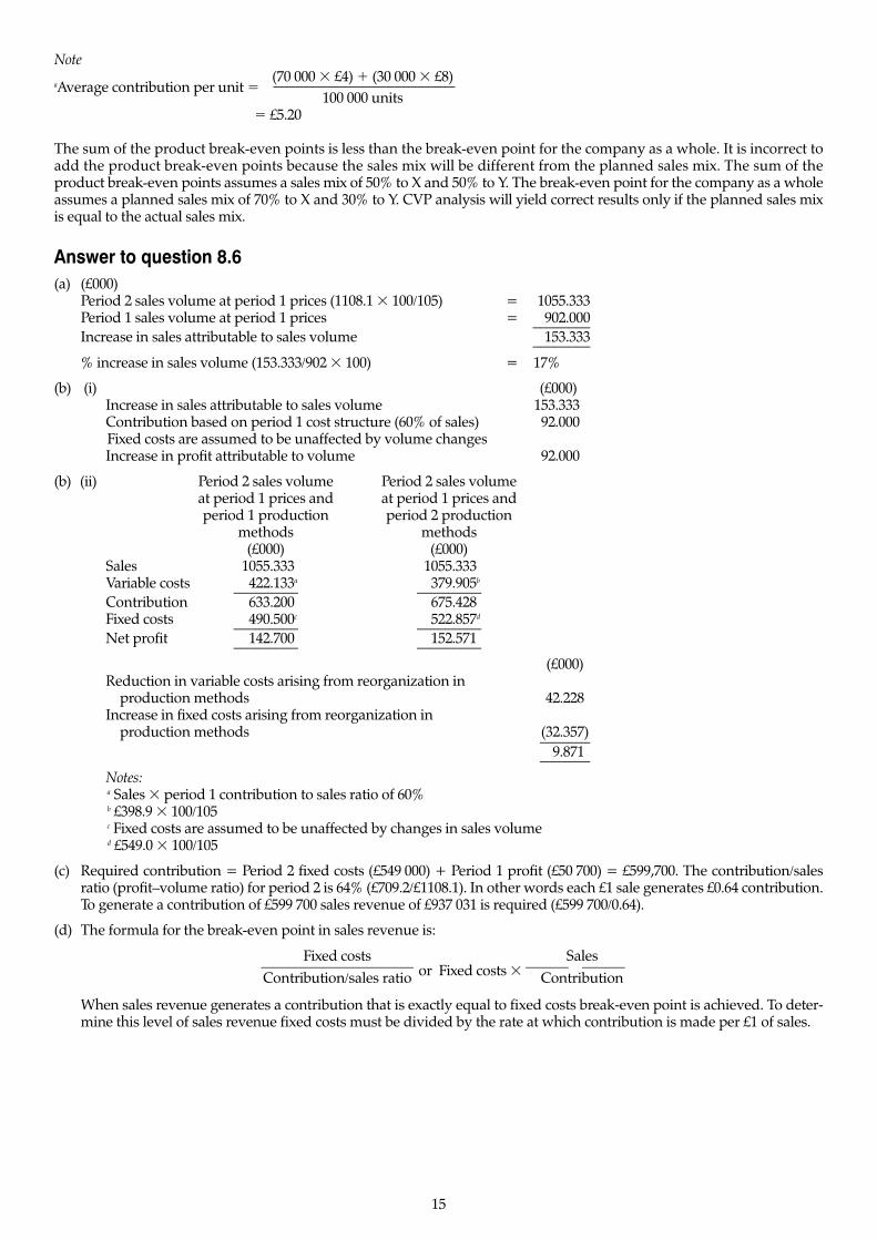
Answer to question 8.6(a) (£000)
Period 2 sales volume at period 1 prices (1108.1 � 100/105) = 1055.333Period 1 sales volume at period 1 prices = 902.000––––––––Increase in sales attributable to sales volume 153.333––––––––% increase in sales volume (153.333/902 � 100) = 17%
(b) (i) (£000)Increase in sales attributable to sales volume 153.333Contribution based on period 1 cost structure (60% of sales) 92.000Fixed costs are assumed to be unaffected by volume changesIncrease in profit attributable to volume 92.000
(b) (ii) Period 2 sales volume Period 2 sales volumeat period 1 prices and at period 1 prices andperiod 1 production period 2 production
methods methods(£000) (£000)
Sales 1055.333 1055.333Variable costs 422.133a 379.905b
––––––––– –––––––––Contribution 633.200 675.428Fixed costs 490.500c 522.857d
––––––––– –––––––––Net profit 142.700 152.571––––––––– –––––––––
(£000)Reduction in variable costs arising from reorganization in
production methods 42.228Increase in fixed costs arising from reorganization in
production methods (32.357)–––––––
9.871–––––––Notes:a Sales � period 1 contribution to sales ratio of 60%b £398.9 � 100/105c Fixed costs are assumed to be unaffected by changes in sales volumed £549.0 � 100/105
(c) Required contribution = Period 2 fixed costs (£549,000) + Period 1 profit (£50,700) = £599,700. The contribution/salesratio (profit–volume ratio) for period 2 is 64% (£709.2/£1108.1). In other words each £1 sale generates £0.64 contribution.To generate a contribution of £599,700 sales revenue of £937,031 is required (£599,700/0.64).
(d) The formula for the break-even point in sales revenue is:
or Fixed costs � �ConStrailbeustion
�
When sales revenue generates a contribution that is exactly equal to fixed costs break-even point is achieved. To deter-mine this level of sales revenue fixed costs must be divided by the rate at which contribution is made per £1 of sales.
Fixed costs���Contribution/sales ratio
15

Answer to question 8.7(a) Budgeted ROCE
Sales Gross profit(£000) (£000)
Accommodation 1350 (45%) 945 (70%)Restaurant 1050 (35%) 210 (20%)Bar 600 (20%) 180 (30%)–––– ––––
3000 1335––––Less fixed costs 565––––Profit before tax 770––––
ROCE 770/7000 � 100 � 11%(b) (i) Required additional profits � £280 000 (4% � £7 million)
Contribution per two-night holiday:
Sales Gross profit % margin Contribution(£) (£) (£)
Accommodation (2 � £25) 50 70 35Restaurant (40% � £50) 20 20 4Bar (20% � £50) 10 30 3––
42––
Number of holidays required to provide a contribution of £280 000 � 6667(£280 000/42)
Number of holidays per week in three off-peak quarters � 171 (6667/39)(£000)
(ii) Required additional contribution 280Contribution arising from increases in selling prices from:
Restaurant (10% � £1 050 000) 105Bar (5% � £600 000) 30 135––– –––
Required additional contribution from accommodation 145–––
Percentage required increase in accommodation prices � 145/1350 � 100� 10.74%
To achieve the desired increase in ROCE, accommodation prices would have to increase by 10.74%. It is assumedthat demand would be unaffected by a price increase of this magnitude.
(c) The major problems arising are:(i) Two-flight cheap holidays
1. Avoiding an increase in fixed costs. For 9 months, the proposal would require 171 additional customers stayingat the hotel each week. Will this increased demand cause an increase in fixed costs (e.g. reception and mainte-nance staff)?
2. The calculations in (a) assume that variable costs vary with sales revenue rather than the number of customers.It is assumed that the gross margin percentage will be the same on cheaper holidays. This implies that the vari-able costs as a percentage of sales revenue will be reduced. It is therefore important that the assumptions madein (a) regarding variable costs being a function of sales revenue are appropriate. An alternative assumption,such as variable costs being a function of the number of guest days, would result in a different answer.
3. Will the introduction of cheap holidays affect the sales volume relating to normal business?(ii) Increasing prices
1. An increase in selling prices may lead to a reduction in demand.2. With this proposal, it is also assumed that variable costs are a function of sales revenue. If variable costs per
guest night were to remain unchanged, the gross profit percentage margin would increase if prices wereincreased.
3. There is a need to obtain more information before increasing prices. For example, when were the prices lastincreased, how does the price increase compare with current levels of inflation, how do the hotel prices com-pare with competitors’ prices?
RecommendationThe assumptions in (a) regarding the percentage reduction in variable costs and no increase in fixed costs arequestionable. Also, a large number of holidays would need to be sold in order to achieve the target ROCE. In contrast,a modest price increase of 10% seems possible without adversely affecting demand. On the basis of the information given, it is recommended that the second alternative be chosen.
16

Answers to questions for Chapter 9 Measuring relevant costs and revenues fordecision-making
Answer to question 9.1(a) Company gross profit % � 38% (£3268/£8600 � 100)
Therefore Division 5 gross profit % � 19%Division 5 sales � £860 000 (10% � £8.6m)Division 5 gross profit � £163 400 (19% � £860 000)Division 5 contribution � £479 400 (£316 000 � £163 400)
The situation for the year ahead if the division were not sold would be as follows:
Contribution � £527 340 (£479 400 � 1.1)Less avoidable fixed costs � £455 700 [£316 000 � (£156 000
� £38 000)] � 1.05Add contribution from other divisions � £20 000–––––––Expected profit £91 640–––––––
If Division 5 were sold, the capital sum would yield a return of £75 400. Therefore the decision on the basis of the aboveinformation should be not to sell Division 5.
(b) Other factors that should influence the decision include:(i) The need to focus on a longer-term time horizon. A decision based solely on the year ahead is too short and
ignores the long-term impact from selling Division 5.(ii) The impact on the morale of the staff working in other divisions arising from the contraction of activities and the
potential threat of redundancies.(iii) Alternative use of the resources currently deployed in Division 5 instead of their current use.
(c) If Division 5 is sold, the capital sum would yield a return of £75 000, but a contribution of £20 000 is lost. Consequently,a profit of £55 000 is required. The required contribution is therefore £510 700 (£55 000 � £455 700) and the percentageincrease required is 6.5% (£510 700/£479 400 � 100%).
Answer to question 9.2(a)
Planned/total contribution and profit for the year ending 31 DecemberRoute W X Y Z Total
(£) (£) (£) (£) (£)Income:Adult 140 400 187 200 351 000 137 280Childa 46 800 74 880 35 100 34 320––––––– ––––––– ––––––– –––––––Total 187 200 262 080 386 100 171 600
Variable costs:Fuel and repairsb 24 570 21 060 25 740 22 230––––––– ––––––– ––––––– –––––––Bus contribution 162 630 241 020 360 360 149 370
Specific fixed costs:Wagesc 74 880 74 880 74 880 74 880Vehicle fixed costs 4 000 4 000 4 000 4 000––––––– ––––––– ––––––– –––––––Route contribution 83 750 162 140 281 480 70 490 597 860––––––– ––––––– ––––––– –––––––General administration 300 000–––––––Profit 297 860–––––––
Notesa 52 weeks × 6 days × 5 journeys per day × number of passengers × return fare × 2 vehiclesb 52 weeks × 6 days × 5 journeys per day × return travel distance × £0.1875 × 2 vehiclesc 52 weeks × 6 days × £120 × 2 vehicles
(b) (i) The relevant (differential) items are the return fares and the average number of passengers per journey:
Adult (£) Child (£)Existing revenue per journey 45 (15 × £3.00) 15 (10 × £1.50)Revised revenue per journey 45 (12 × £3.75) 12 (8 × £1.50)–– ––Net gain/(loss) nil (3)–– ––
The contribution per return journey will decrease by £3.
17

(b) (ii) The above analysis suggests that the fare should not be amended on route W. The only justification is that the cur-rent prices result in the average number of passengers being 25 per journey so it is possible that occasionallydemand may exceed full capacity of 30 passengers resulting in some passengers not being able to be carried. Withthe price increase the average number of passengers will be 20 and it is less likely that some passengers will not beable to be carried.
(c) (i) Annual cost of existing maintenance function(£) (£)
StaffingFitters (£15 808 × 2) 31 616Supervisor 24 000 55 616
–––––Material costsBus servicing (499 200 kma/4000) × £100 12 480Bus safety checks (48 per year at £75) 3 600Taxi servicing (128 000 km/4000 × 6 vehicles) × £100 19 200Taxi safety checks (36 per year at £75) 2 700 37 980
––––– ––––––Total cost 93 596
––––––
Notea 160 km per journey × 5 journeys × 52 weeks × 6 days × 2 vehicles
(c) (ii)(£) (£)
Annual cost of keeping own maintenanceAnnual operating costs 93 596Cost of new employee 20 000 113 596
––––––Annual cost of buying in maintenanceContract cost 90 000Redundancy costs for fitters 15 808 105 808
–––––– ––––––Savings in the first year from buying in maintenance 7 788
––––––
There will be a saving after the first year from buying in maintenance of £23 596 because the redundancy costwill be incurred for one year only.
(c) (iii) AZ will lose control of the operations if the service is carried out externally. It will be more difficult to ensurequality of work and schedule the servicing as required. Once the skills have been lost from outsourcing it maybe difficult to re-establish them. Also AZ will be at the mercy of the supplier when the contract is re-negoti-ated. The extent to which AZ will be dependent on the supplier will be influenced by how competitive themarket is for providing a maintenance service.
AZ could also consider making vehicle servicing a profit centre which competes with external competitorsfor the work of the group.
Answer to question 9.3(a) Hours of installation labour required to satisfy maximum demand
(hours)Day scan: 2000 units × 3 hours per unit 6 000Night scan: 3000 units × 4 hours per unit 12 000Omni scan: 1800 units × 5.5 hours per unit 9 900
––––––27 900
Available hours 25 000––––––
Shortfall 2 900––––––––––––
Note that the labour hours per unit = installation labour cost/£8.
(b) Day scan Night scan Omni scan(£) (£) (£)
Selling price 250 320 460Variable costs
Material (70) (110) (155)Manufacturing labour (40) (55) (70)Installation labour (24) (32) (44)Variable overheads (16) (20) (28)
––– ––– –––Contribution per unit 100 103 163
18
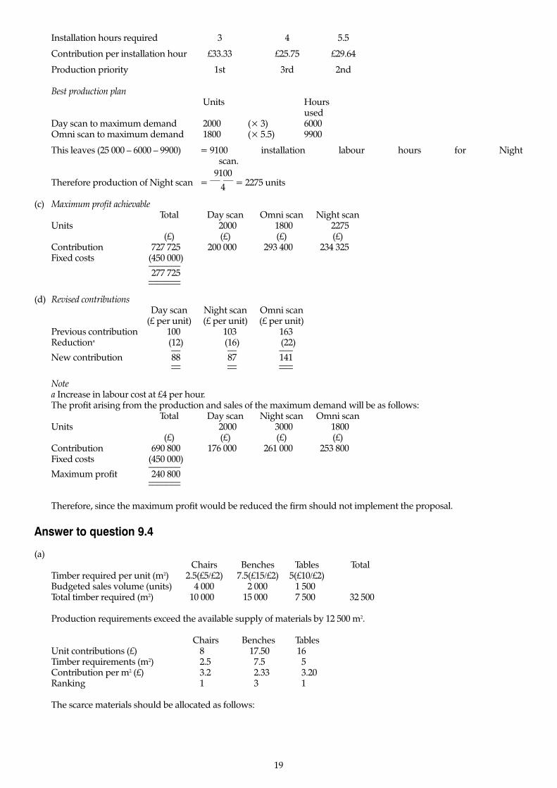
Installation hours required 3 4 5.5
Contribution per installation hour £33.33 £25.75 £29.64
Production priority 1st 3rd 2nd
Best production planUnits Hours
usedDay scan to maximum demand 2000 (× 3) 6000Omni scan to maximum demand 1800 (× 5.5) 9900
This leaves (25 000 – 6000 – 9900) = 9100 installation labour hours for Night scan.
Therefore production of Night scan = �91
400� = 2275 units
(c) Maximum profit achievableTotal Day scan Omni scan Night scan
Units 2000 1800 2275(£) (£) (£) (£)
Contribution 727 725 200 000 293 400 234 325Fixed costs (450 000)
–––––––277 725
––––––––––––––
(d) Revised contributionsDay scan Night scan Omni scan
(£ per unit) (£ per unit) (£ per unit)Previous contribution 100 103 163Reductiona (12) (16) (22)
–– –– –––New contribution 88 87 141
–– –– ––––– –– –––
Notea Increase in labour cost at £4 per hour.The profit arising from the production and sales of the maximum demand will be as follows:
Total Day scan Night scan Omni scanUnits 2000 3000 1800
(£) (£) (£) (£)Contribution 690 800 176 000 261 000 253 800Fixed costs (450 000)
–––––––Maximum profit 240 800
––––––––––––––
Therefore, since the maximum profit would be reduced the firm should not implement the proposal.
Answer to question 9.4
(a)Chairs Benches Tables Total
Timber required per unit (m2) 2.5(£5/£2) 7.5(£15/£2) 5(£10/£2)Budgeted sales volume (units) 4 000 2 000 1 500Total timber required (m2) 10 000 15 000 7 500 32 500
Production requirements exceed the available supply of materials by 12 500 m2.
Chairs Benches TablesUnit contributions (£) 8 17.50 16Timber requirements (m2) 2.5 7.5 5Contribution per m2 (£) 3.2 2.33 3.20Ranking 1 3 1
The scarce materials should be allocated as follows:
19
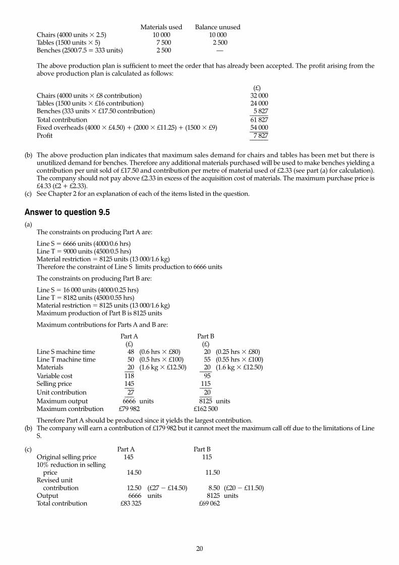
Materials used Balance unusedChairs (4000 units � 2.5) 10 000 10 000Tables (1500 units � 5) 7 500 2 500Benches (2500/7.5 = 333 units) 2 500 —
The above production plan is sufficient to meet the order that has already been accepted. The profit arising from theabove production plan is calculated as follows:
(£)Chairs (4000 units � £8 contribution) 32 000Tables (1500 units � £16 contribution) 24 000Benches (333 units � £17.50 contribution) 5 827––––––Total contribution 61 827Fixed overheads (4000 � £4.50) + (2000 � £11.25) + (1500 � £9) 54 000––––––Profit 7 827––––––
(b) The above production plan indicates that maximum sales demand for chairs and tables has been met but there isunutilized demand for benches. Therefore any additional materials purchased will be used to make benches yielding acontribution per unit sold of £17.50 and contribution per metre of material used of £2.33 (see part (a) for calculation).The company should not pay above £2.33 in excess of the acquisition cost of materials. The maximum purchase price is£4.33 (£2 + £2.33).
(c) See Chapter 2 for an explanation of each of the items listed in the question.
Answer to question 9.5(a)
The constraints on producing Part A are:
Line S � 6666 units (4000/0.6 hrs)Line T � 9000 units (4500/0.5 hrs)Material restriction � 8125 units (13 000/1.6 kg)Therefore the constraint of Line S limits production to 6666 units
The constraints on producing Part B are:
Line S � 16 000 units (4000/0.25 hrs)Line T � 8182 units (4500/0.55 hrs)Material restriction � 8125 units (13 000/1.6 kg)Maximum production of Part B is 8125 units
Maximum contributions for Parts A and B are:
Part A Part B(£) (£)
Line S machine time 48 (0.6 hrs � £80) 20 (0.25 hrs � £80)Line T machine time 50 (0.5 hrs � £100) 55 (0.55 hrs � £100)Materials 20 (1.6 kg � £12.50) 20 (1.6 kg � £12.50)––– ––––Variable cost 118 95Selling price 145 115––– ––––Unit contribution 27 20––– ––––Maximum output 6666 units 8125 unitsMaximum contribution £79 982 £162 500
Therefore Part A should be produced since it yields the largest contribution.(b) The company will earn a contribution of £179 982 but it cannot meet the maximum call off due to the limitations of Line
S.
(c) Part A Part BOriginal selling price 145.00 115.0010% reduction in selling
price 14.50 11.50Revised unit
contribution 12.50 (£27 � £14.50) 8.50 (£20 � £11.50)Output 6666 units 8125 unitsTotal contribution £83 325 £69 062
20

Payment for unusedmachine hoursa £70 020 £120 000–––––––– ––––––––
Revised contribution £153 345 £189 062–––––––– ––––––––
NoteaThe payment for unused machine hours is calculated as follows:
Part A(£)
Line S at £60 per hour — (Fully used)Line T at £60 per hour 70 020 (4500 � [6666 � 0.5 hrs])––––––
70 020––––––
Part B(£)
Line S at £60 per hour 118 125 (4000 � [8125 � 0.25 hrs])Line T at £60 per hour 1 875 (4500 � [8125 � 0.55 hrs])–––––––
120 000–––––––
With the alternative pricing arrangement the company should produce Part B.
Answer to question 9.6(a) Maximum production of each product is as follows:
Traditional ModernMachine X hour limitation 6800 (1700/0.25) 11 333 (1700/0.15)Machine Y hour limitation 9600 (1920/0.20) 8 533 (1920/0.225)Timber (m2 limitation) 8500 (17 000/2) 8 500 (17 000/2)Maximum sales 7400 10 000Maximum possible production 6800 8 500
The contribution per unit of output is:
Traditional ModernVariable costs: (£) (£)
Timber 5.00 5.00Machine X 6.25 (0.25 � £25) 3.75 (0.15 � £25)Machine Y 6.00 (0.20 � £30) 6.75 (0.225 � £30)––––– –––––
17.25 15.50Selling price 45.00 40.00––––– –––––Contribution 27.75 24.50––––– –––––
Assuming that only one of the products can be sold the maximum contribution from the sales of each product is:
Traditional £188 700 (6800 � £27.75)Modern £208 250 (8500 � £24.50)
The company should therefore sell 8500 units of the ‘Modern’ lampstand.(b) The spare machine capacity assuming that 6800 units of the ‘Traditional’ lamp-stand or 8500 of the ‘Modern’
lampstand are produced is as follows:
Machine X Machine Y(Hours) (Hours)
Production of 6800of Traditional Nil [1700 � (6800 � 0.25)] 560 [1920 � (6800 � 0.20)]
Production of 8500of Modern 425 [1700 � (8500 � 0.15)] 7.5 [1920 � (8500 � 0.225)]
The revised contributions are:
Traditional Modern(£) (£)
Original contribution 188 700 208 250Sales from unused capacity of
machine X Nil 8 500 (425 � £20)
21
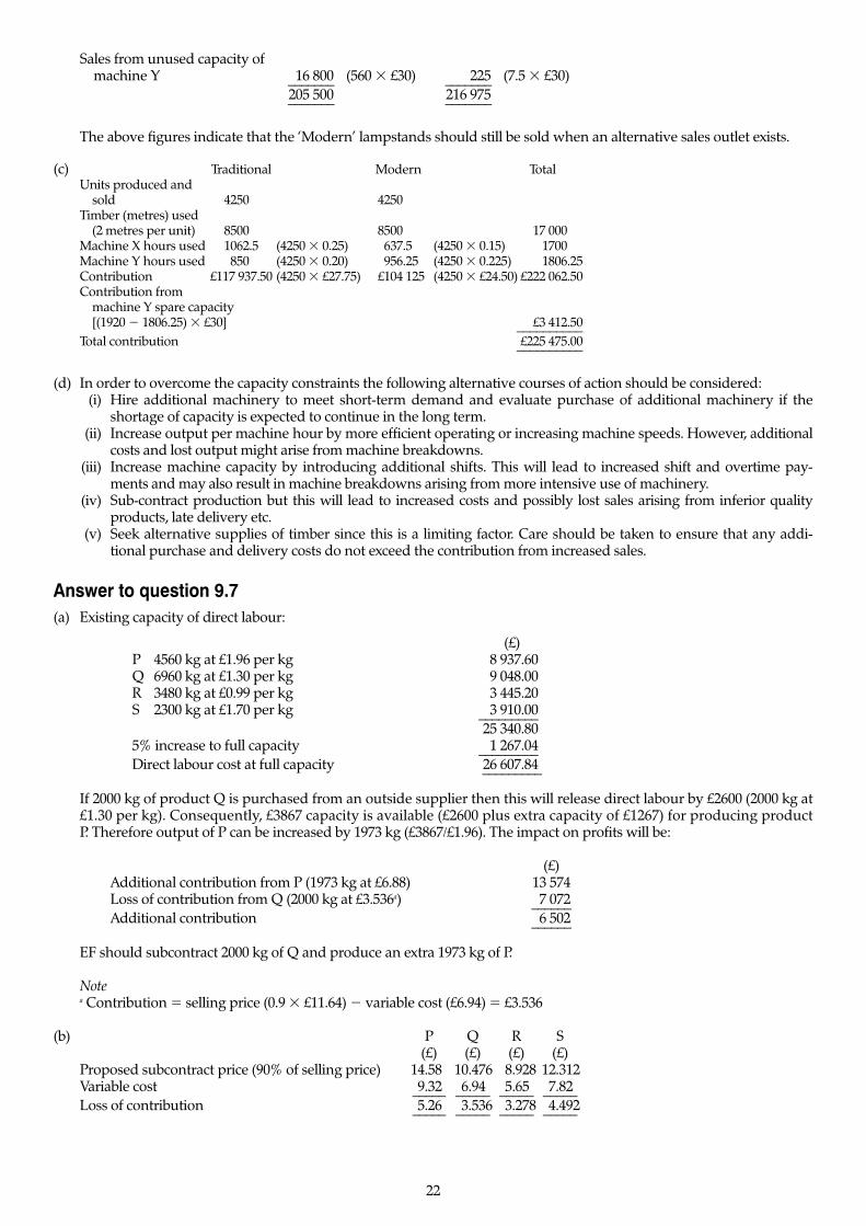
Sales from unused capacity ofmachine Y 16 800 (560 � £30) 225 (7.5 � £30)––––––– –––––––
205 500 216 975––––––– –––––––
The above figures indicate that the ‘Modern’ lampstands should still be sold when an alternative sales outlet exists.
(c) Traditional Modern TotalUnits produced and
sold 4250.5 4250Timber (metres) used
(2 metres per unit) 8500.5 8500.5 17 000.50Machine X hours used 1062.5 (4250 � 0.25) 637.5 (4250 � 0.15) 1700.50Machine Y hours used 850.5 (4250 � 0.20) 956.25 (4250 � 0.225) 1806.25Contribution £117 937.50 (4250 � £27.75) £104 125 (4250 � £24.50) £222 062.50Contribution from
machine Y spare capacity[(1920 � 1806.25) � £30] £3 412.50––––––––––
Total contribution £225 475.00––––––––––
(d) In order to overcome the capacity constraints the following alternative courses of action should be considered:(i) Hire additional machinery to meet short-term demand and evaluate purchase of additional machinery if the
shortage of capacity is expected to continue in the long term.(ii) Increase output per machine hour by more efficient operating or increasing machine speeds. However, additional
costs and lost output might arise from machine breakdowns.(iii) Increase machine capacity by introducing additional shifts. This will lead to increased shift and overtime pay-
ments and may also result in machine breakdowns arising from more intensive use of machinery.(iv) Sub-contract production but this will lead to increased costs and possibly lost sales arising from inferior quality
products, late delivery etc.(v) Seek alternative supplies of timber since this is a limiting factor. Care should be taken to ensure that any addi-
tional purchase and delivery costs do not exceed the contribution from increased sales.
Answer to question 9.7(a) Existing capacity of direct labour:
(£)P 4560 kg at £1.96 per kg 8 937.60Q 6960 kg at £1.30 per kg 9 048.00R 3480 kg at £0.99 per kg 3 445.20S 2300 kg at £1.70 per kg 3 910.00–––––––––
25 340.805% increase to full capacity 1 267.04–––––––––Direct labour cost at full capacity 26 607.84–––––––––
If 2000 kg of product Q is purchased from an outside supplier then this will release direct labour by £2600 (2000 kg at£1.30 per kg). Consequently, £3867 capacity is available (£2600 plus extra capacity of £1267) for producing product P. Therefore output of P can be increased by 1973 kg (£3867/£1.96). The impact on profits will be:
(£)Additional contribution from P (1973 kg at £6.88) 13 574Loss of contribution from Q (2000 kg at £3.536a) 7 072––––––Additional contribution 6 502––––––
EF should subcontract 2000 kg of Q and produce an extra 1973 kg of P.
Notea Contribution � selling price (0.9 � £11.64) � variable cost (£6.94) � £3.536
(b) P Q R S(£) (£) (£) (£)
Proposed subcontract price (90% of selling price) 14.58 10.476 8.928 12.312Variable cost 9.32 6.94 5.65 7.82––––– ––––– ––––– –––––Loss of contribution 5.26 3.536 3.278 4.492––––– ––––– ––––– –––––
22
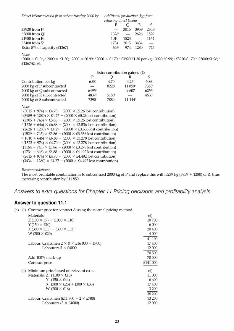
Direct labour released from subcontracting 2000 kg Additional production (kg) fromreleasing direct labour
P Q R S£3920 from Pa — 3015e 3959f 2305g
£2600 from Qb 1326h — 2626 1529£1980 from Rc 1010 1523 — 1164£3400 from Sd 1734 2615 3434 —Extra 5% of capacity (£1267) 646i 974 1280 745
Notesa2000 � £1.96; b 2000 � £1.30; c 2000 � £0.99; d 2000 � £1.70; e £3920/£1.30 per kg; f 3920/£0.99; g £3920/£1.70; h £2600/£1.96; i
£1267/£1.96.
Extra contribution gained (£)P Q R S
Contribution per kg 6.88 4.70 4.27 5.862000 kg of P subcontracted — 8228a 11 850b 7353c
2000 kg of Q subcontracted 6495d — 9 607e 6253f
2000 kg of R subcontracted 4837g 5180h — 4630i
2000 kg of S subcontracted 7390j 7884k 11 144l —
Notesa (3015 � 974) � £4.70 � (2000 � £5.26 lost contribution)b (3959 � 1280) � £4.27 � (2000 � £5.26 lost contribution)c (2305 � 745) � £5.86 � (2000 � £5.26 lost contribution)d (1326 � 646) � £6.88 � (2000 � £3.536 lost contribution)e (2626 � 1280) � £4.27 � (2000 � £3.536 lost contribution)f (1529 � 745) � £5.86 � (2000 � £3.536 lost contribution)g (1010 � 646) � £6.88 � (2000 � £3.278 lost contribution)h (1523 � 974) � £4.70 � (2000 � £3.278 lost contribution)i (1164 � 745) � £5.86 � (2000 � £3.278 lost contribution)j (1734 � 646) � £6.88 � (2000 � £4.492 lost contribution)k (2615 � 974) � £4.70 � (2000 � £4.492 lost contribution)l (3434 � 1280) � £4.27 � (2000 � £4.492 lost contribution)
Recommendations:The most profitable combination is to subcontract 2000 kg of P and replace this with 5239 kg (3959 � 1280) of R, thusincreasing contribution by £11 850.
Answers to extra questions for Chapter 11 Pricing decisions and profitability analysis
Answer to question 11.1(a) (i) Contract price for contract A using the normal pricing method.
Materials (£)Z (100 � £7) � (1000 � £10) 10 700Y (150 � £40) 6 000X (300 � £35) � (300 � £33) 20 400W (200 � £20) 4 000––––––––
41 100Labour: Craftsmen 2 � (�� � £16 000 � £700) 17 400Labour: Labourers 3 � £4000 12 000––––––––
70 500Add 100% mark-up 70 500––––––––Contract price £141 000––––––––
(ii) Minimum price based on relevant costs (£)Materials: Z (1100 � £10) 11 000
Y (150 � £44) 6 600X (300 � £25) � (300 � £33) 17 400W (200 � £16) 3 200––––––
38 200Labour: Craftsmen (£11 800 � 2 � £700) 13 200Labour: Labourers (3 � £4000) 12 000
23
Equipment: General purpose (£16 400 � £12 600) 3 800Equipment: Specialized (£9000 � £5800) 3 200Administrative expenses 5 000––––––Contract price 75 400––––––
It is assumed that the specialized equipment would be purchased new for £9000.
(b) (£)Expected sales value (0.7 � £100 000) � (0.3 � £120 000) 106 000)Expected building costs (0.4 � £60 000) � (0.4 � £80 000)
� (0.2 � £95 000) (75 000)Building plot (20 000)––––––––Expected profit 11 000)––––––––Using expected profit as a measure of the alternative use of the capacity, the minimum price using the relevant costapproach would be £86 400 (£75 400 � £11 000). In other words, Wright would wish to ensure that the contract price is in excess of the profit available from the alternative use of the facilities, and this would depend on his assessment ofthe ‘utility value’ of project B. Note that the expected value approach is covered in Chapter 12.
(c) This question requires a discussion of cost-plus pricing and the relevant cost (that is, opportunity cost) approach topricing. For a discussion of the limitations and merits of cost-plus pricing see ‘Limitations of cost-plus pricing’ and‘Reasons for using cost-based pricing formulae’ in Chapter 11. The advantages of basing selling prices on relevant costsinclude:
(i) The alternative uses of resources are incorporated into the analysis.(ii) It distinguishes between relevant and irrelevant costs and indicates the incremental cash flows incurred in manu-
facturing and selling a product.(iii) It provides the information to enable tenders to be made at more competitive prices.The limitations include:
(i) It is a cost-based pricing method that ignores demand.(ii) It may provide an incentive to sell at low prices, resulting in total sales revenue being insufficient to cover total
fixed costs.(iii) There is difficulty in determining the opportunity cost of resources because information on available opportuni-
ties may not be known.(iv) Where special contracts are negotiated that are in excess of relevant (incremental) costs but less than full costs,
there is a danger that customers will expect repeat business at this selling price. Care must be taken to ensure thatnegotiating ‘special one-off ’ contracts does not affect the demand for other products.
Relevant cost pricing is more appropriate for ‘one-off ’ pricing decisions. It is also appropriate in situations wherea firm has unutilized capacity or can sell in differentiated markets at different prices. Relevant cost pricing mayalso be appropriate where the policy is to sell certain products as ‘loss leaders’. It is important that cost informationbe used in a flexible manner and that product costs not be seen as the only factor that should determine the finalselling price.
Answer to question 11.2(a) Selling prices using the existing policy of full cost 1 5%
Cost of 1250 filter elements (£)Direct labour 18 750Materials 43 750Variable overhead 12 500––––––Variable cost (£60 per unit) 75 000Fixed overhead 5 000Fixed packaging and selling cost 7 000––––––
87 000––––––
Full cost per filter element � �£8
1725
0000
� � £69.60
Full cost per complete unit � £69.60 � £305 � £374.60Using full cost � 5%, rounded up to nearest £1:Selling price for complete unit � £374.60 � 1.05 � £394.00Selling price for replacement elements � £69.60 � 1.05 � £74.00
(b) At a selling price of 20% above the market leader for the replacement filter sales of the complete units will not beaffected. Therefore the maximum price of £96 (£80 � 1.20) should be charged for replacement filters.
At a selling price of £280 demand is expected to be 800 units (40% � 2000). Each increase in price of £1 causesdemand to fall by 5 units. Therefore at a selling price of £440 demand will be zero. To increase demand by one unit theselling price must be reduced by £0.20. Thus the maximum selling price for an output of x units is:
24
SP � £440 � £0.20xTotal revenue for an output of x units � £440x � £0.20x2
Marginal revenue � dTR/dx � £440 � £0.40xTotal cost � 305x � 60x � £5000 � £7000Marginal cost � £365
The sale of one complete unit results in the sale of four replacement filters during its life at a marginal revenue of £96and a marginal cost of £60 per unit.
Total MC � £365 � (4 � £60) � £605Total MR � £440 � 0.4x � (4 � £96) � £824 � 0.4xAt the optimal output level where MR � MC:£824 � 0.4x � £605
x � 548 units
This gives a selling price of £440 � 0.20 (548) � £330.40
(c) Original selling price
The profit for each of the years would be constant:
(£) (£)Sales: complete units 250 @ £394 98 500)
replacement elements 1000 @ £74 74 000)––––––––172 500)
Variable costs: pumps 250 @ £305 76 250)other 1250 @ £60 75 000––––––
(151 250)––––––––Contribution 21 250)Fixed costs: (12 000)––––––––Profit 9 250)––––––––
Revised selling price
2002 2003 2004(£) (£) (£) (£) (£) (£)
Revenues:Complete units548 @ £330.40 181 059.20) 181 059.20) 181 059.20)Replacementelements @ £96a 96 000.00) 124 608.00) 153 216.00)––––––––––– ––––––––––– –––––––––––
277 059.20) 305 667.20) 334 275.20)
Variable costs:Complete units548 @ £305 167 140 167 140 167 140Replacementelements @£60a 92 880 110 760 128 640––––––– –––––––– ––––––––
(260 020.00) (277 900.00) (295 780.00)––––––––––– ––––––––––– –––––––––––17 039.20 27 767.20 38 495.20
Fixed costs (12 000.00) (12 000.00) (12 000.00)––––––––––– ––––––––––– –––––––––––Profit 5 039.20 15 767.20 26 495.20––––––––––– ––––––––––– –––––––––––Change in profits (4210.80) 6 517.20 17 245.20
NoteaThe number of replacement filters will increase over the next four years because they are replaced at the end of eachyear (four times during their lifetime). Therefore sales of replacement filters are related to sales in previous periods.The question also states that production of replacement filters must be sufficient to meet annual sales demand plus theproduction of a filter to be included in the sale of one completed unit. Thus production of filters will exceed sales by548 filters per year. The sales and production volumes of replacement filters is calculated as follows:
2002 Sales (Based on previous year’s sales volume) 1000Production (1000 � 548) 1548
25
2003 Sales � (�� � 1000) � (�� � [548 � 4]) 1298Production (1298 � 548) 1846
2004 Sales � (�� � 1000) � (�� � [548 � 4]) 1596Production (1596 � 548) 2144
(d) The major competitor has set the selling price at £390 and the traditional cost-plus method results in a selling price of£394. The proposed new selling price is £330.40. The major concern with setting the new price is the possible reaction of competitors. Given that the total market is stable, a large decrease in selling price to increase market share is likely tocause competitors to reduce prices. This could result in a price cutting war in which market shares are merelymaintained at lower prices. In the long term the company might be worse off.
A further problem is that the lower price may be perceived by customers as indicating an inferior quality product.Customers might therefore be reluctant to switch from their existing suppliers.
To overcome these problems the price reduction should be accompanied with an effective advertising campaign thatemphasizes the price and quality aspects of the product.
(e) For the answer to this question see ‘Limitations and Cost-plus pricing’ and ‘Reasons for using cost-plus prices’ inChapter 11.
Answers to extra questions for Chapter 12 Decision-making under conditions of risk oruncertainty
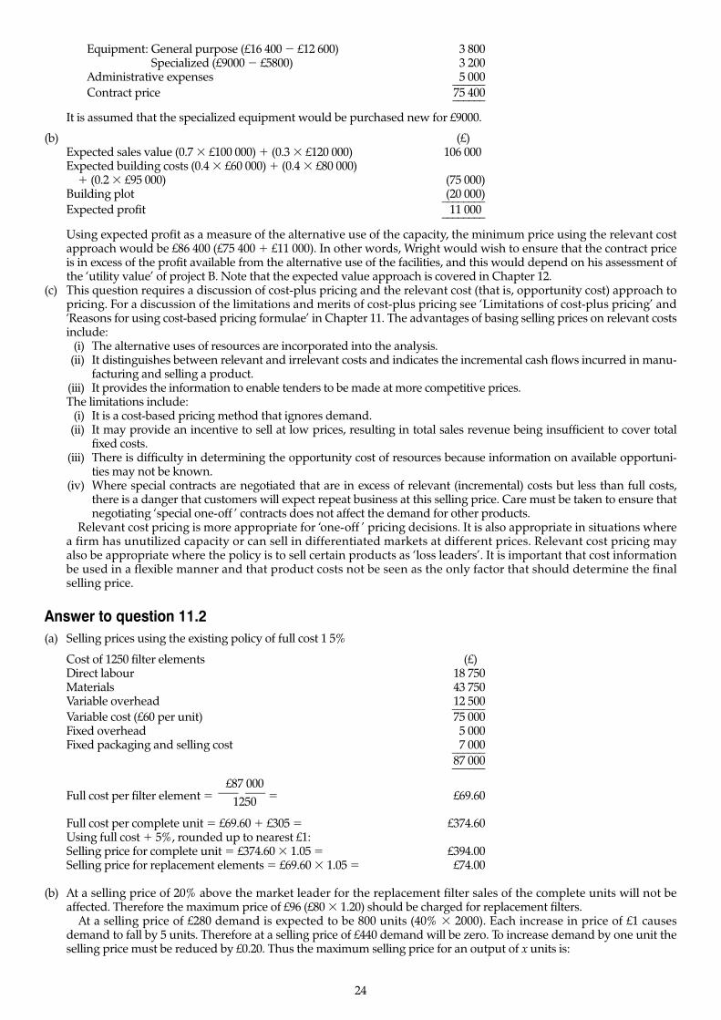
Answer to question 12.18(a) Decision tree and expected value calculation for site A
See Figure Q12.18.
Year 0 Year 1 Year 2 Joint ExpectedCash flows Cash flows Cash flows probability PV NPV
(£) (£)0 0.0625 90 910 5 628
(0.25)
£100 000 £100 000 0.125 173 550 21 694
(0.25) (0.50)
£200 000 0.0625 256 190 16 012
(0.25)
£100 000 0.125 264 640 33 080
(0.25)
Investment £200 000 £200 000 0.25 347 100 86 775
outlay (£300 000) (0.50) (0.50)
£300 000 0.125 429 740 53 718
(0.25)
£200 000 0.0625 438 010 27 376
(0.25)
£300 000 £300 000 0.125 520 650 65 081
(0.25) (0.50)
£350 000 0.0625 561 970 35 123–––– –––––(0.25) 1.000 344 487––––
Less investment outlay 300 000–––––Expected NPV 44 487–––––
Figure Q12.18 Decision tree and expected value calculation for site A.
(b) (i) It is assumed that the decision to abandon the project can be taken at the end of year 1. At this point in time, thecash flows for year 2 will be receivable in one year’s time, whereas the sale proceeds will be receivable at the pointwhen the decision is taken at the end of year 1. Therefore the decision should be to abandon the project if the PVof the cash flows receivable in one year’s time is less than the £150 000 selling price. If the cash inflows in year 1 are£100 000 then the expected PV of the cash flows in year 2 will be:
Cash flows PV Probability Expected PV(£) (£) (£)
100 000 90 910 0.50 45 455200 000 181 820 0.25 45 455––––––
90 910––––––
26
The site should therefore be sold for £150 000. If the cash flow for year 1 is £200 000, the expected PV of the cashinflows in year 2 will be:
Cash flows PV Probability Expected NPV(£) (£) (£)
100 000 90 910 0.25 22 727200 000 181 820 0.50 90 910300 000 272 730 0.25 68 182–––––––
181 819–––––––
The expected NPV is in excess of the sale proceeds, and therefore the project should not be abandoned.(ii) If the cash flow in year 1 is £100 000 then the project will be abandoned and sold for £150 000 at the end of year 1.
Therefore there is a probability of 0.25 that £250 000 will be received at the end of year 1. Hence the expected NPVwill be £56 819. Therefore the entries in the expected value column of the decision tree in (a) for the first threebranches (£5628, £21 694 and £16 012, totalling £43 334) will be replaced with an expected value of £56 819. Hencethe total expected value will increase by £13 485 to £57 972 (£13 485 � £44 487).
(c) At time zero the financial effect is that the NPV of the project is increased by £13 485.
Answers to extra questions for Chapter 13 Capital investment decisions: 1
Answer to question 13.1(a) The answer should stress that NPV is considered superior to the payback method and the accounting rate of return
because it takes account of the time value of money. For a description of the time value of money you should refer to‘Compounding and discounting’ and ‘The concept of net present value’ in Chapter 13. The answer should also drawattention to the limitations of the payback method and accounting rate of return described in Chapter 13.
(b) (i) To compute the NPV it is necessary to convert the profits into cash flows by adding back depreciation of £25 000per annum in respect of the asset purchased at the end of year 3 for £75 000. The NPV calculation is as follows:
Year Cash flow Discount factor NPV(£)
3 (75 000) 0.675 (50 625)4 35 000 0.592 20 7205 28 000 0.519 14 5326 27 000 0.465 12 555––––––
(2 818)––––––
(ii) The cash flows are based on the assumption that the reinvestment in R is not made at the end of year 3.
Discount Project T Project T Project R Project RYear factor cash flowsa NPV cash flows NPV
(£) (£) (£) (£)1 0.877 27 000 23 679 40 000 (3)c 35 0802 0.769 30 000 23 070 45 000 34 6053 0.675 32 000 21 600 45 000 (4)d 30 3754 0.592 44 000 26 0485 0.519 40 000b 20 760––––––– –––––––
115 157 100 060Investment outlay 70 000 60 000––––––– –––––––
NPV 45 157 40 060––––––– –––––––
Payback: T � 2 years � (£70 000 � £57 000)/£32 000 � 2.41 yearsR � 1 year � (£60 000 � £40 000)/45 000 � 1.44 years
The decision should be to invest in Project T because it has the higher NPV.
NotesaYearly profits plus (£70 000 � £10 000)/5 years depreciation.b£18 000 profits � £12 000 depreciation � £10 000 sale proceeds.cProfits plus £60 000/3 years depreciation.d£75 000 investment outlay � £50 000 � Annual profit (£25 000). Cash flow � £25 000 profit � £20 000depreciation.
(c) For an explanation of the meaning of the term ‘discount rate’ see ‘The opportunity cost of an investment’ in Chapter 13.
27
The discount rate can be derived from observations of the returns shareholders require in financial markets. Where aproject is to be financed fully by borrowing, the cost of borrowing could be used as a basis for determining thediscount rate.
Answer to question 13.2(a) The PV of the cash outflows is calculated as follows:
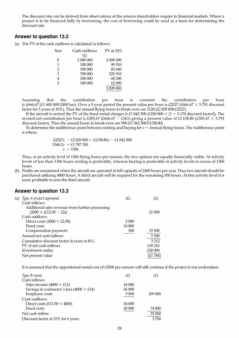
Year Cash outflows PV at 10%(£)
0 2 000 000 2 000 0001 100 000 90 9102 100 000 82 6403 700 000 525 9104 100 000 68 3005 100 000 62 090–––––––––
2 829 850–––––––––
Assuming that the contribution per hour is constant the contribution per hour is £666.67 (£1 600 000/2400 hrs). Over a 5-year period the present value per hour is £2527 (£666.67 � 3.791 discountfactor for 5 years at 10%). Thus the annual flying hours to break even are 1120 (£2 829 850/£2527).
If the aircraft is rented the PV of the fixed rental charges is £1 042 500 (£250 000 � [1 � 3.170 discount factor]). Therevised net contribution per hour is £305.67 (£666.67 � £361) giving a present value of £1 158.80 (£305.67 � 3.791discount factor). Thus the annual hours to break even are 900 (£1 042 500/£1158.80).
To determine the indifference point between renting and buying let x � Annual flying hours. The indifference pointis where:
£2527x � £2 829 850 � £1158.80x � £1 042 5001368.2x � £1 787 350
x � 1306
Thus, at an activity level of 1306 flying hours per annum, the two options are equally financially viable. At activitylevels of less than 1306 hours renting is preferable, whereas buying is preferable at activity levels in excess of 1306hours.
(b) Profits are maximized when the aircraft are operated at full capacity of 2400 hours per year. Thus two aircraft should bepurchased utilizing 4800 hours. A third aircraft will be required for the remaining 950 hours. At this activity level it ismore profitable to rent the third aircraft.
Answer to question 13.3(a) Type A project appraisal (£) (£)
Cash inflows:Additional sales revenue from further processing
(2000 � (£12.50 � £2)) 21 000)Cash outflows:
Direct costs (2000 � £2.50) 5 000Fixed costs 10 000Compensation payment 500 15 500)–––––– ––––––––
Annual net cash inflows 5 500)––––––––Cumulative discount factor (4 years at 8%) 3.312)PV of net cash inflows £18 216)Investment outlay £20 000)––––––––Net present value (£1 784)––––––––
It is assumed that the apportioned rental cost of £2500 per annum will still continue if the project is not undertaken.
Type B waste (£) (£)Cash inflows:
Sales income (4000 � £11) 44 000Savings in contractor’s fees (4000 � £14) 56 000Employee costs 9 000 109 000––––––
Cash outflows:Direct costs (£13.50 � 4000) 54 000Fixed costs 20 000 74 000–––––– ––––––––
Net cash inflow 35 000––––––––Discount factor at 15% for 6 years 3.784
28

Present value of net cash inflows £132 440Investment outlay
(£120 000 � sale of containers at £18 000) £102 000––––––––Net present value £ 30 440––––––––
The project should therefore not be accepted.The above analysis is based on the assumption that the contract for the sale of the product lasts for 6 years. If the
customer does not renew the contract at the end of 4 years, the present value of the net cash inflows will be reduced by£40 898 [£44 000 � (0.4972 � 0.4323)]. This would result in a negative NPV of £10 458 (£30 440 � £40 898) plus anydisposal cost of the unwanted product. On the other hand, if the company can sell more than 1023 units of the product [£10 458/(£11 � 0.9295)] in years 5 and 6, the project will have a positive NPV.
The project should be accepted if management are optimistic that the contract will be renewed or are confident thatmore than 1023 units can be sold in each of years 5 and 6.
(b) The major reservations about the project for Type B waste are as follows:(i) There could be additional redundancy costs if the existing employee is made redundant. If the employee is not
made redundant, there might not be any cash flow savings.(ii) The technology is new, and operating problems that cannot be foreseen might arise.(iii) The present system seems to work satisfactorily. Will there be any additional risks, given that the process is haz-
ardous, with the extra processing?
Answer to question 13.4(a) The current return on capital employed is 20% (£20m profit/(£75m fixed assets + £25m stocks))
The computation of the capital employed for the new project is calculated as follows:
Year 1 2 3 4(£m) (£m) (£m) (£m)
Sales 10.0 (£5 × 2m) 8.10 (£4.50 × 1.8m) 6.40 (£4 × 1.6m) 5.60 (£3.50 × 1.6m)Op. cost (2.00) (1.80) (1.60) (1.60)Fixed costs (1.50) (1.35) (1.20) (1.20)Depreciation (3.00) (3.00) (3.00) (3.00)
–––– –––– –––– ––––Profit 3.50 1.95 0.60 (0.20)
Capital employed (start-of-year):
Fixed 14.00 11.00 8.00 5.00Stocks 0.50 0.50 0.50 0.50
–––– –––– –––– ––––Total 14.50 11.50 8.50 5.50
Average profits = Total profits of £5.85m/4 years = £1.46mAverage capital employed = Capital employed at the mid point of the project’s life (i.e. capital employed at thestart of year 3) = £8.50m
Alternatively the average capital employed can be calculated as indicated in Chapter 13 (i.e. initial cost of theequipment of £14m plus the estimated residual value of £2m multiplied by 0.5 giving £8m). The investment instocks is £0.5m so the total average investment is £8.5m.
Average rate of return = £1.46m/£8.5m = 17.2%
The proposal has an expected return in excess of the minimum of 10% specified by the company but it is unlikely thatthe manager will submit the proposal for approval because the proposed return is less than the current average of20%. If the proposed project is undertaken the overall average return will be less than 20%. For an explanation of thispoint you should refer to ‘The effect of performance measurement on capital investment decisions’ in Chapter 13.
(b) (i) The following problems arise with the use of the average accounting rate of return on capital employed.(i) It ignores the time value of money.
(ii) Accounting profits are used rather than cash flows. Both depreciation and fixed costs are not cash flows andwould not be incorporated in a NPV calculation.
(iii) The accounting rate of return can be expressed in a variety of ways and it is therefore subject to manipulation.For example, different methods of depreciation will produce different average rates of return.
(b) (ii) The accounting return on capital employed (also known as return on investment) is widely used by financial mar-kets to evaluate the performance of the company as a whole. Because of this top management are likely to be inter-ested in the impact that the project will have on the overall return on capital employed of the company. Theaccounting return on capital employed on proposed projects provides this information. Also many managers areevaluated on the overall return of their divisions on capital employed. If this is the case, it is likely that managerswill focus on the return on capital employed of individual projects. Thus the way that performance is measured islikely to have a profound effect on the criteria that is used to appraise projects. For a more detailed explanation ofthis point see ‘The effect of performance measurement on capital investment decisions’ in Chapter 13.
29

Answer to question 13.5(a) Incremental operating costs
Output Machine X Machine Y(000 units) (£000) (£000)
10 53 4320 80 5730 96 6640 122 139
Minimum cost tableMachine X Machine Y Total
Output Output Cost Output Cost cost(000 units) (000 units) (£000) (000 units) (£000) (£000)
10 — — 10 43 4320 — — 20 57 5730 — — 30 66 6640 10 53 30 66 11950 20 80 30 66 14660 30 96 30 66 16270 40 122 30 66 18880 40 122 40 139 261
(b) (i) Profitability
Output Sales Costs Contribution(000 units) (£000) (£000) (£000)
10 60 43 1720 120 57 6330 180 66 11440 240 119 12150 300 146 15460 360 162 19870 420 188 23280 480 261 219
Profits are maximized at an output level of 70 000 units.(ii) At an output level of 40 000 units machine X has the lowest cost. Machine Y should therefore be offered for sale. It
is assumed that if machine Y is not sold, the output from the two machines over the next five years would be 60 000 units (75% � 80 000). The financial effect of selling machine Y would be as follows:
Two machines Machine X only(60 000 units) (40 000 units)
(£) (£)Sales 360 000 240 000Costs 162 000 122 000–––––––– ––––––––Contribution 198 000 118 000Add annual cost savings 45 000–––––––– ––––––––
198 000 163 000–––––––– ––––––––It is assumed that the company would save £45 000 (£65 000 � £20 000) direct costs in other sections of the com-pany if machine Y were sold. Annual future cash flows would therefore decline by £35 000 (£198 000 � £163 000).The PV of £35 000 annual cash flows for 5 years is £123 095 (£35 000 � 3.517). In addition, there would be a loss ofscrap value of £20 000 in year 5. The PV of £20 000 receivable in year 5 is £10 856. Therefore the PV of the lost cashflows if machine Y was sold is £133 951 (£123 095 � £10 856). The minimum selling price is £134 000.
(c) Other factors that should be considered are:(i) The impact of disruption of supplies if machine X breaks down. With two machines, the company can meet
urgent orders if one machine breaks down. With only one machine, there is a distinct possibility that the companywill fail to meet delivery dates if machine X breaks down.
(ii) The effect of not being able to meet the annual demand of 60 000 units per annum from LC Ltd. What is the likeli-hood that LC Ltd will seek another supplier?
(iii) It is assumed that the company will save £45 000 direct expenses elsewhere in the company if machine Y is sold.In practice, such savings might not be made, or may be made gradually. It is important that the company estab-lishes the likely savings over the five-year period prior to negotiating a selling price with LC Ltd.
30
Answer to question 13.6(a) The present values of the capital costs are as follows:
Discount PresentYear Staff Expenses Contingency Total factor value
(£000) (£)1 20 5 2.5 27.5 0.8772 24 1232 22 5 2.5 29.5 0.7695 22 7003 24 5 2.5 31.5 0.675 21 2624 26 5 2.5 33.5 0.5921 19 8355 28 5 2.5 35.5 0.5194 18 439–––––––
106 359Initial outlay 60 000–––––––
166 359–––––––
Let x � required net annual incomeTherefore the PV of the net annual income over 5 years equates with the PV of the capital costs, where:
0.35 � 0.8772x � 0.65 � 0.7695x � 0.675x � 0.5921x � 0.5194x � £166 3592.593x � £166 359
x � £64 155
If net income is 50% of sales then food sales would need to be £128 310 (£64 155 � 2) in years 3–5. Therefore annualsales required are:
(£)Year 1 44 908 (0.35 � £128 310)
2 83 401 (0.65 � £128 310)3 128 3104 128 3105 128 310
(b) Aspects of the proposal that might merit further consideration include:(i) Is the 14% discount rate equivalent to the opportunity cost of funds allocated by the Management Board?
(ii) Prices, potential demand and product range need to be considered. What is the probability that total income willbe sufficient to generate the sales revenue specified in (a)?
(iii) How does the proposed product range, service and price structure compare with other catering facilities availablewithin the locality?
(iv) Is there sufficient expertise and time available for existing staff to operate the new facilities?(v) What alternative uses are available for the surplus accommodation?
Answers to extra questions for Chapter 14 Capital investment decisions: 2
Answer to question 14.1The report should include the information contained in items (a) to (c) below:(a) Depreciation is not a cash flow. The operating net cash inflows (before tax) therefore consist of sales less materials
and labour costs. The NPV calculation is as follows:Year 0 1 2 3 4
(£) (£) (£) (£) (£)Net cash inflows before tax 80 000 75 000 69 750Taxa (14 025) (15 469) 4826Investment outlay (150 000)
Net cash flow (150 000) 80 000 60 975 54 281 4826Discount factor (18%) 1.000 0.847 0.718 0.609 0.516Present value (150 000) 67 760 43 780 33 057 2490
NPV = �£2 913
31

Note:The tax computation is as follows:Year 1 2 3
(£) (£) (£)Net cash inflows before tax 80 000 75 000 69 750Writing down allowances 37 500 28 125 84 375Taxable profit 42 500 46 875 (14 625)Tax at 33% 14 025 15 469 (4 826)Writing down allowances:Opening WDV 150 000 112 500 84 375Writing down allowances (25%) 37 500 28 125Closing WDV 112 500 84 375 NilBalancing allowance 84 375
(b) Because corporation taxes are payable on taxable profits and not accounting profits depreciation has been replaced bythe Inland Revenue’s allowable depreciation (known as written-down allowances). The net cost of the asset is £150 000and written-down allowances received amounted to £65 625 (£37 500 + £28 125). Therefore a balancing allowance isavailable at the end of the asset’s life of £84 375 (£150 000 � £65 625). The Inland Revenue allows the net cost of theasset to be claimed over its life with a balancing adjustment in the final year. Because taxation is normally payable 9months after the company’s accounting year end the taxation cash flows are shown to be delayed by one year. This is asimplification of the actual situation but is normally sufficiently accurate for appraising investments.
(c) Other factors to be considered include:(i) The probability of obtaining a subsequent contract. There would be no need to purchase a further machine and
the project would therefore yield a positive NPV.(ii) The negative NPV is very small and if the company has other profitable activities it may be worthwhile accepting
in order to have the chance of obtaining a second contract and establishing long-term relationships with a largemultinational customer.
(iii) Capacity that is available. If other profitable opportunities have to be forgone to undertake the contract because ofshortage of capacity then the opportunity cost should be included in the financial analysis.
Answer to question 14.2
PV of cost of operating new machines
(£)Purchase price (£52 000 � 4) 208 000)PV of annual operating costs for 7 years (£15 000 � 4 � 4.564) 273 840)Salvage value (4 � £4000 � 0.4523) (7 237)––––––––PV of costs over 7-year life 474 603)––––––––––––––––
PV of costs £474 603Equivalent annual cost �
annuity factor for n years at R%�
4.564= £103 988
PV of cost of operating old machine
(£)Opportunity cost of selling machines (10 � £5000) 50 000Operating costs (10 � £10 000 � 2.402) 240 200–––––––PV of costs over 3-year life 290 200–––––––
Equivalent annual cost (£290 200/2.402) � £120 816
The new machines have the lowest equivalent annual cost. Therefore they should be replaced now. This decision is basedon the assumption that no superior or cheaper machines will be available in three years’ time. If other opportunities arelikely to be available in three years’ time then the combination of operating the old machines and replacing with more effi-cient or cheaper machines should be considered.
The costs of modifying the factory building should be compared with the savings that result from the installation of thenew machines. Equivalent annual savings from purchasing the new machines are £16 828 (£120 816 � £103 988) for threeyears. The PV of these savings is £40 421 (£16 828 � 2.402). It is assumed that if the factory is not modified now, it will haveto be modified in three years’ time when the current machines reach the end of their life. Assuming the cost of modifica-tion will still be £60 000 in three years’ time, the relevant cost of the modification is:
32
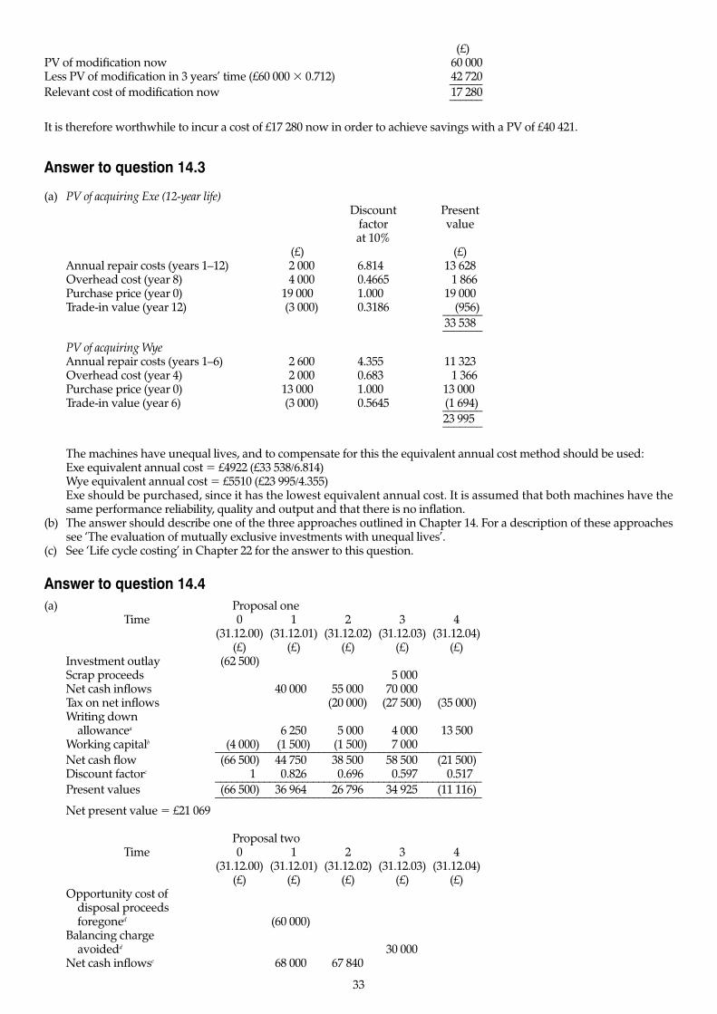
(£)PV of modification now 60 000Less PV of modification in 3 years’ time (£60 000 � 0.712) 42 720––––––Relevant cost of modification now 17 280––––––
It is therefore worthwhile to incur a cost of £17 280 now in order to achieve savings with a PV of £40 421.
Answer to question 14.3
(a) PV of acquiring Exe (12-year life)Discount Present
factor valueat 10%
(£) (£)Annual repair costs (years 1–12) 2 000 6.8140 13 628Overhead cost (year 8) 4 000 0.4665 1 866Purchase price (year 0) 19 000 1.0000 19 000Trade-in value (year 12) (3 000) 0.3186 (956)–––––––
33 538–––––––PV of acquiring WyeAnnual repair costs (years 1–6) 2 600 4.3550 11 323Overhead cost (year 4) 2 000 0.6830 1 366Purchase price (year 0) 13 000 1.0000 13 000Trade-in value (year 6) (3 000) 0.5645 (1 694)–––––––
23 995–––––––
The machines have unequal lives, and to compensate for this the equivalent annual cost method should be used:Exe equivalent annual cost � £4922 (£33 538/6.814)Wye equivalent annual cost � £5510 (£23 995/4.355)Exe should be purchased, since it has the lowest equivalent annual cost. It is assumed that both machines have thesame performance reliability, quality and output and that there is no inflation.
(b) The answer should describe one of the three approaches outlined in Chapter 14. For a description of these approachessee ‘The evaluation of mutually exclusive investments with unequal lives’.
(c) See ‘Life cycle costing’ in Chapter 22 for the answer to this question.
Answer to question 14.4(a) Proposal one
Time 0 1 2 3 4(31.12.00) (31.12.01) (31.12.02) (31.12.03) (31.12.04)
(£) (£) (£) (£) (£)Investment outlay (62 500)Scrap proceeds 5 000)Net cash inflows 40 000) 55 000) 70 000)Tax on net inflows (20 000) (27 500) (35 000)Writing down
allowancea 6 250) 5 000) 4 000) 13 500)Working capitalb (4 000) (1 500) (1 500) 7 000)–––––––––––––––––––––––––––––––––––––––––––––––––Net cash flow (66 500) 44 750) 38 500) 58 500) (21 500)Discount factorc 1) 0.826) 0.696) 0.597) 0.517)–––––––––––––––––––––––––––––––––––––––––––––––––Present values (66 500) 36 964) 26 796) 34 925) (11 116)–––––––––––––––––––––––––––––––––––––––––––––––––Net present value � £21 069
Proposal twoTime 0 1 2 3 4
(31.12.00) (31.12.01) (31.12.02) (31.12.03) (31.12.04)(£) (£) (£) (£) (£)
Opportunity cost ofdisposal proceedsforegoned (60 000)
Balancing chargeavoidedd 30 000)
Net cash inflowse 68 000) 67 840)
33
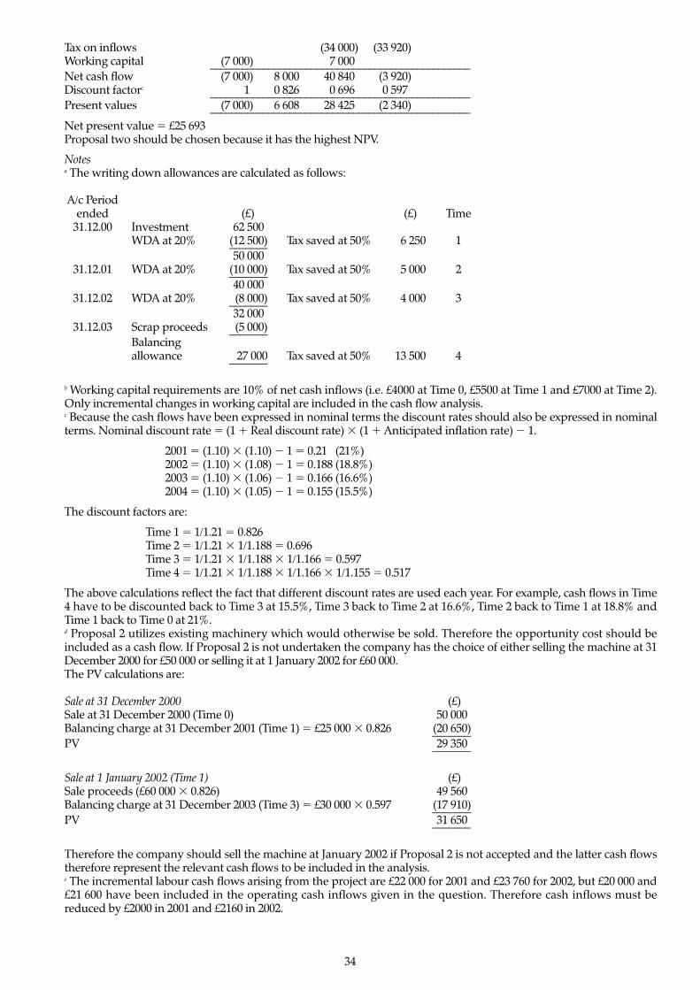
Tax on inflows (34 000) (33 920)Working capital (7 000) 7 000)–––––––––––––––––––––––––––––––––––––––––––––––––Net cash flow (7 000) 8 000) 40 840) (3 920)Discount factorc 1) 0 826) 0 696) 0 597)–––––––––––––––––––––––––––––––––––––––––––––––––Present values (7 000) 6 608) 28 425) (2 340)–––––––––––––––––––––––––––––––––––––––––––––––––Net present value � £25 693Proposal two should be chosen because it has the highest NPV.
Notesa The writing down allowances are calculated as follows:
A/c Periodended (£) (£) Time
31.12.00 Investment 62 500)WDA at 20% (12 500) Tax saved at 50% 6 250 1–––––––
50 000)31.12.01 WDA at 20% (10 000) Tax saved at 50% 5 000 2–––––––
40 000)31.12.02 WDA at 20% (8 000) Tax saved at 50% 4 000 3–––––––
32 000)31.12.03 Scrap proceeds (5 000)–––––––
Balancingallowance 27 000 Tax saved at 50% 13 500 4–––––––
b Working capital requirements are 10% of net cash inflows (i.e. £4000 at Time 0, £5500 at Time 1 and £7000 at Time 2).Only incremental changes in working capital are included in the cash flow analysis.c Because the cash flows have been expressed in nominal terms the discount rates should also be expressed in nominalterms. Nominal discount rate � (1 � Real discount rate) � (1 � Anticipated inflation rate) � 1.
2001 � (1.10) � (1.10) � 1 � 0.21 (21%)2002 � (1.10) � (1.08) � 1 � 0.188 (18.8%)2003 � (1.10) � (1.06) � 1 � 0.166 (16.6%)2004 � (1.10) � (1.05) � 1 � 0.155 (15.5%)
The discount factors are:
Time 1 � 1/1.21 � 0.826Time 2 � 1/1.21 � 1/1.188 � 0.696Time 3 � 1/1.21 � 1/1.188 � 1/1.166 � 0.597Time 4 � 1/1.21 � 1/1.188 � 1/1.166 � 1/1.155 � 0.517
The above calculations reflect the fact that different discount rates are used each year. For example, cash flows in Time4 have to be discounted back to Time 3 at 15.5%, Time 3 back to Time 2 at 16.6%, Time 2 back to Time 1 at 18.8% andTime 1 back to Time 0 at 21%.d Proposal 2 utilizes existing machinery which would otherwise be sold. Therefore the opportunity cost should beincluded as a cash flow. If Proposal 2 is not undertaken the company has the choice of either selling the machine at 31December 2000 for £50 000 or selling it at 1 January 2002 for £60 000.The PV calculations are:
Sale at 31 December 2000 (£)Sale at 31 December 2000 (Time 0) 50 000)Balancing charge at 31 December 2001 (Time 1) � £25 000 � 0.826 (20 650)–––––––PV 29 350)–––––––
Sale at 1 January 2002 (Time 1) (£)Sale proceeds (£60 000 � 0.826) 49 560)Balancing charge at 31 December 2003 (Time 3) � £30 000 � 0.597 (17 910)–––––––PV 31 650)–––––––
Therefore the company should sell the machine at January 2002 if Proposal 2 is not accepted and the latter cash flowstherefore represent the relevant cash flows to be included in the analysis.e The incremental labour cash flows arising from the project are £22 000 for 2001 and £23 760 for 2002, but £20 000 and£21 600 have been included in the operating cash inflows given in the question. Therefore cash inflows must bereduced by £2000 in 2001 and £2160 in 2002.
34
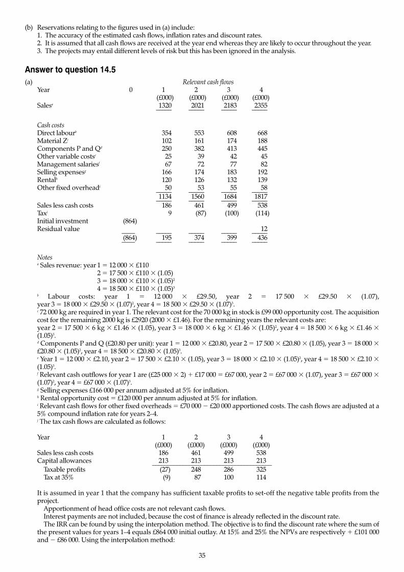
(b) Reservations relating to the figures used in (a) include:1. The accuracy of the estimated cash flows, inflation rates and discount rates.2. It is assumed that all cash flows are received at the year end whereas they are likely to occur throughout the year.3. The projects may entail different levels of risk but this has been ignored in the analysis.
Answer to question 14.5(a) Relevant cash flows
Year 0 1 2 3 4(£000) (£000) (£000) (£000)
Salesa 1320 2021 2183 2355––––– ––––– ––––– –––––
Cash costsDirect labourb 354 553) 608) 668)Material Zc 102 161) 174) 188)Components P and Qd 250 382) 413) 445)Other variable costse 25 39) 42) 45)Management salariesf 67 72) 77) 82)Selling expensesg 166 174) 183) 192)Rentalh 120 126) 132) 139)Other fixed overheadi 50 53) 55) 58)––––– ––––– ––––– –––––
1134 1560) 1684) 1817)––––– ––––– ––––– –––––Sales less cash costs 186 461) 499) 538)Taxj 9 (87) (100) (114)Initial investment (864)Residual value 12)–––– ––––– ––––– ––––– –––––
(864) 195 374) 399) 436)–––– ––––– ––––– ––––– –––––
Notesa Sales revenue: year 1 � 12 000 � £110
2 � 17 500 � £110 � (1.05)3 � 18 000 � £110 � (1.05)2
4 � 18 500 � £110 � (1.05)3
b Labour costs: year 1 � 12 000 � £29.50, year 2 � 17 500 � £29.50 � (1.07), year 3 � 18 000 � £29.50 � (1.07)2, year 4 � 18 500 � £29.50 � (1.07)3.c 72 000 kg are required in year 1. The relevant cost for the 70 000 kg in stock is £99 000 opportunity cost. The acquisitioncost for the remaining 2000 kg is £2920 (2000 � £1.46). For the remaining years the relevant costs are:year 2 � 17 500 � 6 kg � £1.46 � (1.05), year 3 � 18 000 � 6 kg � £1.46 � (1.05)2, year 4 � 18 500 � 6 kg � £1.46 �(1.05)3.d Components P and Q (£20.80 per unit): year 1 � 12 000 � £20.80, year 2 � 17 500 � £20.80 � (1.05), year 3 � 18 000 �£20.80 � (1.05)2, year 4 � 18 500 � £20.80 � (1.05)3.e Year 1 � 12 000 � £2.10, year 2 � 17 500 � £2.10 � (1.05), year 3 � 18 000 � £2.10 � (1.05)2, year 4 � 18 500 � £2.10 �(1.05)3.f Relevant cash outflows for year 1 are (£25 000 � 2) � £17 000 � £67 000, year 2 � £67 000 � (1.07), year 3 � £67 000 �(1.07)2, year 4 � £67 000 � (1.07)3.g Selling expenses £166 000 per annum adjusted at 5% for inflation.h Rental opportunity cost � £120 000 per annum adjusted at 5% for inflation.i Relevant cash flows for other fixed overheads � £70 000 � £20 000 apportioned costs. The cash flows are adjusted at a5% compound inflation rate for years 2–4.j The tax cash flows are calculated as follows:
Year 1 2 3 4(£000) (£000) (£000) (£000)
Sales less cash costs 186 461 499 538Capital allowances 213 213 213 213–––––––––––––––––––––––––––––––––––––––
Taxable profits (27) 248 286 325Tax at 35% (9) 87 100 114
It is assumed in year 1 that the company has sufficient taxable profits to set-off the negative table profits from theproject.
Apportionment of head office costs are not relevant cash flows.Interest payments are not included, because the cost of finance is already reflected in the discount rate.The IRR can be found by using the interpolation method. The objective is to find the discount rate where the sum of
the present values for years 1–4 equals £864 000 initial outlay. At 15% and 25% the NPVs are respectively � £101 000and � £86 000. Using the interpolation method:
35
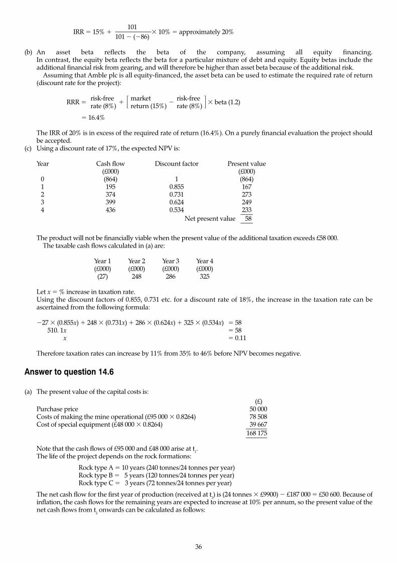
101IRR � 15% �
101 � (�86)� 10% � approximately 20%
(b) An asset beta reflects the beta of the company, assuming all equity financing. In contrast, the equity beta reflects the beta for a particular mixture of debt and equity. Equity betas include theadditional financial risk from gearing, and will therefore be higher than asset beta because of the additional risk.
Assuming that Amble plc is all equity-financed, the asset beta can be used to estimate the required rate of return(discount rate for the project):
RRR � risk-free�
market�
risk-free� beta (1.2)rate (8%) � return (15%) rate (8%) �
� 16.4%
The IRR of 20% is in excess of the required rate of return (16.4%). On a purely financial evaluation the project shouldbe accepted.
(c) Using a discount rate of 17%, the expected NPV is:
Year Cash flow Discount factor Present value(£000) (£000)
0 (864) 1 (864)1 195 0.855 1672 374 0.731 2733 399 0.624 2494 436 0.534 233––––
Net present value 58––––
The product will not be financially viable when the present value of the additional taxation exceeds £58 000.The taxable cash flows calculated in (a) are:
Year 1 Year 2 Year 3 Year 4(£000) (£000) (£000) (£000)(27) 248 286 325
Let x � % increase in taxation rate.Using the discount factors of 0.855, 0.731 etc. for a discount rate of 18%, the increase in the taxation rate can beascertained from the following formula:
�27 � (0.855x) � 248 � (0.731x) � 286 � (0.624x) � 325 � (0.534x) � 58510. 1x � 58
x � 0.11
Therefore taxation rates can increase by 11% from 35% to 46% before NPV becomes negative.
Answer to question 14.6
(a) The present value of the capital costs is:(£)
Purchase price 50 000Costs of making the mine operational (£95 000 � 0.8264) 78 508Cost of special equipment (£48 000 � 0.8264) 39 667–––––––
168 175–––––––
Note that the cash flows of £95 000 and £48 000 arise at t1.
The life of the project depends on the rock formations:
Rock type A � 10 years (240 tonnes/24 tonnes per year)Rock type B � 5 years (120 tonnes/24 tonnes per year)Rock type C � 3 years (72 tonnes/24 tonnes per year)
The net cash flow for the first year of production (received at t2) is (24 tonnes � £9900) � £187 000 � £50 600. Because of
inflation, the cash flows for the remaining years are expected to increase at 10% per annum, so the present value of thenet cash flows from t
2onwards can be calculated as follows:
36
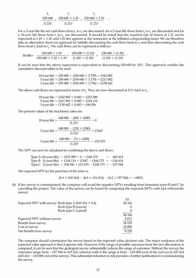
t2
t3
t4
£50 600�
£50 600 � 1.10�
£50 600 � 1.10 …––––––– ––––––––––––– –––––––––––––(1.21)2 (1.21)3 (1.21)4
For a 3-year life the net cash flows from t2to t
4are discounted, for a 5-year life those from t
2to t
6are discounted and for
a 10-year life those from t2
to t11
are discounted. It should be noted that the required rate of return of 1.21 can beexpressed as 1.10 � 1.10, and 1.10 also appears in the numerator as the inflation compounding factor. We can thereforetake an alternative short-cut approach by initially discounting the cash flows back to t
2and then discounting the cash
flows from t2back to t
0. The cash flows can be expressed as follows:
50 600�£50 600 � 1.10
�£50 600 � (1.10)2
�£50 600 � (1.10)3 …
£50 600 � 1.10 � 1.10 (1.10)2 � (1.10)2 (1.10)3 � (1.10)3
It can be seen that the above expression is equivalent to discounting £50 600 by 10%. This approach enables thecumulative discount tables to be used.
10-year life � £50 600 � (£50 600 � 5.759) � £342 0055-year life � £50 600 � (£50 600 � 3.170) � £211 0023-year life � £50 600 � (£50 600 � 1.736) � £138 442
The above cash flows are expressed in terms of t2. They are now discounted at 21% back to t
0.
10-year life � £342 005 � 0.683 � £233 5895-year life � £211 002 � 0.683 � £144 1143-year life � £138 442 � 0.683 � £94 556
The present values of the machinery sales are:
10-year life �£48 000 � (240 � £200)
� 0(1.21)11
5-year life �£48 000 � (120 � £200)
� £7647(1.21)6
3-year life �£48 000 � (72 � £200)
� £15 675(1.21)4
The NPV can now be calculated by combining the above cash flows:
Type A (10-year life) � £233 589 � 0 � £168 175 � £65 414Type B (5-year life) � £144 114 � £7647 � £168 175 � �£16 414Type C (3-year life) � £94 556 � £15 675 � £168 175 � �£57 944
The expected NPV for the purchase of the mine is:
(0.4 � £65 414) � (0.4 � £16 414) � (0.2 � £57 944) � �£8011
(b) If the survey is commissioned, the company will avoid the negative NPVs resulting from formation types B and C bycancelling the project. The value of the survey can be found by comparing the expected NPVs with and without thesurvey:
(£)Expected NPV with survey: Rock type A (£65 414 � 0.4) 26 166
Rock type B (cancel) 0Rock type C (cancel) 0––––––
26 166Expected NPV without survey 8 011––––––Benefit from survey 18 155Cost of survey 10 000––––––Net benefit from survey 8 155––––––
The company should commission the survey based on the expected value decision rule. The major weakness of theexpected value approach is that it ignores risk. However, if the range of possible outcomes from the two alternatives iscompared, it can be seen that the geological survey substantially reduces the range of outcomes. Without the survey, theoutcomes range from �£57 944 to £65 414, whereas with it the range is from �£10 000 (cost of the survey) to £55 414 (£65 414 � £10 000 cost of the survey). This substantial reduction in risk provides a further justification for commissioningthe survey.
37
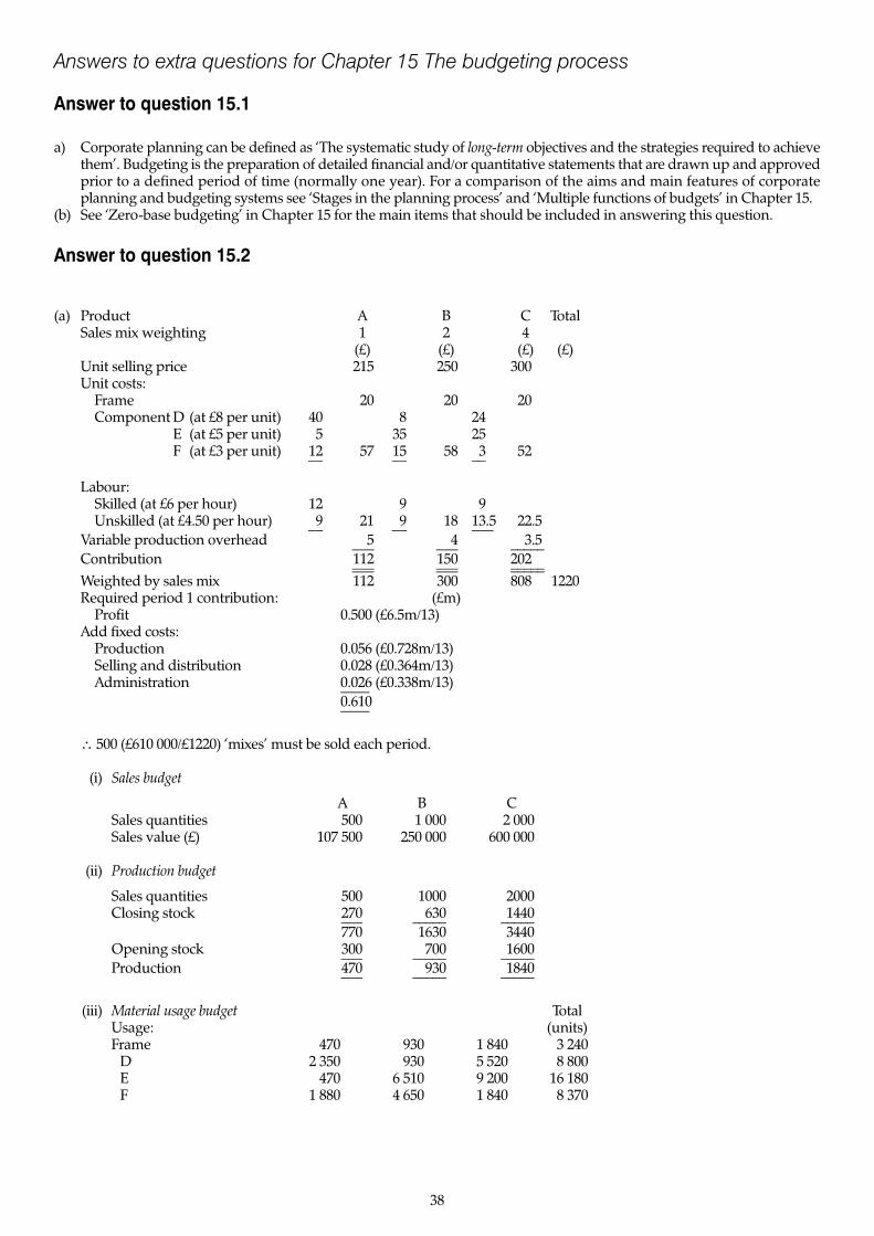
Answers to extra questions for Chapter 15 The budgeting process
Answer to question 15.1
a) Corporate planning can be defined as ‘The systematic study of long-term objectives and the strategies required to achievethem’. Budgeting is the preparation of detailed financial and/or quantitative statements that are drawn up and approvedprior to a defined period of time (normally one year). For a comparison of the aims and main features of corporateplanning and budgeting systems see ‘Stages in the planning process’ and ‘Multiple functions of budgets’ in Chapter 15.
(b) See ‘Zero-base budgeting’ in Chapter 15 for the main items that should be included in answering this question.
Answer to question 15.2
(a) Product A B C TotalSales mix weighting 1 2 4
(£) (£) (£) (£)Unit selling price 215 250 300Unit costs:
Frame 20 20 20Component D (at £8 per unit) 40 8 24
E (at £5 per unit) 5 35 25F (at £3 per unit) 12 57 15 58 3 52–– –– ––
Labour:Skilled (at £6 per hour) 12 9 9Unskilled (at £4.50 per hour) 9 21 9 18 13.5 22.5–– –– –––
Variable production overhead 5 4 3.5––– ––– –––––Contribution 112 150 202––– ––– –––––––– ––– –––––Weighted by sales mix 112 300 808 1220Required period 1 contribution: (£m)
Profit 0.500 (£6.5m/13)Add fixed costs:
Production 0.056 (£0.728m/13)Selling and distribution 0.028 (£0.364m/13)Administration 0.026 (£0.338m/13)––––
0.610––––
∴ 500 (£610 000/£1220) ‘mixes’ must be sold each period.
(i) Sales budget
A B CSales quantities 500 1 000 2 000Sales value (£) 107 500 250 000 600 000
(ii) Production budget
Sales quantities 500 1000 2000Closing stock 270 630 1440––– ––––– –––––
770 1630 3440Opening stock 300 700 1600––– ––––– –––––Production 470 930 1840––– ––––– –––––
(iii) Material usage budget TotalUsage: (units)Frame 470 930 1 840 3 240
D 2 350 930 5 520 8 800E 470 6 510 9 200 16 180F 1 880 4 650 1 840 8 370
38
(iv) Purchases budget
Purchases (units): Frame D E FClosing stock 900 3 600 9 000 3 600Add used in production 3 240 8 800 16 180 8 370–––––– –––––– –––––– ––––––
4 140 12 400 25 180 11 970Less opening stock 1 000 4 000 10 000 4 000–––––– –––––– –––––– ––––––Purchases (units) 3 140 8 400 15 180 7 970–––––– –––––– –––––– ––––––Cost (£) 62 800 67 200 75 900 23 910
(v) Manpower budgets Machining Assembly(hours) (hours)
A (units produced � hrs per unit) 940 940B 1395 1860C 2760 5520–––– ––––
5095 8320Hours available per period (4 � 37.5) 150 150Number of people required 34 56
(b) The following factors would need to be considered:(i) The ability to be able to plan future production requirements, since production might be halted if there was a sud-
den increase in production. If production is volatile, there is a danger that stockouts might occur.(ii) The speed and reliability of the delivery service. If suppliers can deliver at short notice then stockouts are less
likely to occur.(iii) The extra costs involved arising from more frequent deliveries in terms of ordering costs and quantity discounts.(iv) Alternative use of storage space.(v) The savings in holding costs arising from the reduction in stocks. Stock reductions in units would be as follows:
Frames D E FEnd of
period 1 900 3600 9000 3600Requirements
for 1 week 810 (3240/4) 2200 (8800/4) 4045 (16 180/4) 2092 (8370/4)–––––––––––––––––––––––––––––––––––––––––––––––––––––––Stock
reduction 90 1400 4955 1508–––––––––––––––––––––––––––––––––––––––––––––––––––––––
Answer to question 15.3Task 1
(a) Production budget – third quarter ending 17 SeptemberAlphas Betas
Budgeted sales in units 2000 2400Add closing stocka 200 480Less opening stock (given) (500) (600)
–––––– ––––––Production of completed units 1700 2280
–––––– ––––––
(b) Materials purchases budget – third quarter ending 17 Septemberkilograms
Material required for Alpha production (8kg × 1700) 13 600Material required for Beta production (12kg × 2280) 27 360
––––––40 960
Add closing material stockb 16 384Less opening material stock (given) (12 000)
––––––Material purchases 45 344
––––––
(c) Cost of material purchases (45 344 × £10) £453 440
(d) Labour budget – third quarter ending 17 SeptemberLabour hours required for Alpha production (3 hours × 1700) 5 100Labour hours required for Beta production (6 hours × 2280) 13 680
––––––Total hours required before efficiency adjustment 18 780Efficiency adjustment (20%/
80%) 4 695
––––––Total labour hours 23 475
39
Normal hours (50 employees × 35 hours × 12 weeks) 21 000––––––
Overtime hours 2 475––––––
(e) Normal hours (50 employees × 12 weeks × £210) £126 000Overtime (2475 hours × £9) £22 275
––––––––Cost of labour £148 275
––––––––
Notes Alphas BetasaSales this quarter 2000 2400Add 20% seasonal variation 400 480
–––––– ––––––Budgeted sales next quarter 2400 2880
–––––– ––––––Closing stock (5/60 × 2400 = 200) (10/60 × 2880 = 480) 200 480bClosing stock of materialsProduction this period 40 960Add 20% 8 192
––––––Material required for production next period 49 152
––––––Stock required (20/60 × 49 152) 16 384
Task 2
(a) Some of the following limitations should be included in the report: (i) Past data are normally used as a basis for determining the linear regression formula. If only a small number of
past observations are available the resulting regression formula is not likely to be very accurate.(ii) The technique assumes that a linear relationship exists whereas in practice a curvilinear relationship may exist.
(iii) If past data are used to make future predictions it is assumed that the past trend will continue into the future.However, past trends may suddenly change for a variety of reasons.
(iv) If abnormal observations are included in past data the regression equation will not be typical of future normalrelationships.
Task 2
(b) The report should identify the following alternative methods of forecasting: (i) Market research involving customer surveys of likely future demand.
(ii) Obtaining estimates from salespersons who deal with the customers and who have the knowledge to predictfuture demand.
Note that linear regression is dealt with in Chapter 24.
Answer to question 15.4(a) Monthly cash budget
Month 1 Month 2 Month 3 Month 4(£000) (£000) (£000) (£000)
Cash inflows:Sales (W1) 24.0 93.6 92.6 90.7–––– –––– –––– –––––––– –––– –––– ––––
Cash outflows:Business purchase 315.0 — — —Delivery van — 15.0 — —Raw materials (W2) — 44.375 29.375 30.625Direct labour (W2) 27.0 17.25 18.0 18.75Production overhead (W3) 10.5 10.5 10.5 10.5Selling and administration
overhead (W4) 39.875 14.875 14.875 14.875–––––––– –––––––– –––––––– ––––––––392.375 102.0 72.75 74.75
Surplus/(deficit) for month (368.375) (8.4) 19.85 15.95Opening balance — (368.375) (376.775) (356.925)Closing balance (368.375) (376.775) (356.925) (340.975)
Workings
40
Month 1 Month 2 Month 3 Month 4(W1) Cash inflow from sales 24 24 23 24––– –––– –––– ––––
Cash inflow from credit sales — 72 72 69Less discount — (2.4) (2.4) (2.3)––– –––– –––– ––––
— 69.6 69.6 66.7––– –––– –––– ––––Total cash inflow 24 93.6 92.6 90.7––– –––– –––– ––––
(W2) Selling price at a mark-up of 60% on production cost is £8 per unit(£5.00 � 1.60).
Sales units � sales revenue/8.(000 units) Month 1 Month 2 Month 3 Month 4 Month 5 Month 6Sales 12 12 11.5 12 12.5 13
� Closing stock offinished goods 12 11.5 12 12.5 13
� Opening stock offinished goods 6 12 11.5 12 12.5–––– –––– –––– –––– ––––
� Production 18 11.5 12 12.5 13� Closing stock of raw
materials 5.75 6 6.25 6.5� Opening stock of raw
materials 6 5.75 6 6.25–––– –––– –––– ––––� Purchase of raw
materials 17.75 11.75 12.25 12.75–––– –––– –––– ––––Raw material cost (£000) Month 1 Month 2 Month 3 Month 4
� Purchases at £2.50 44.375 29.375 30.265 31.875Raw material payment (£000) — 44.375 29.375 30.625Direct labour cost and payment (£000)
� Production � £1.50 27 17.25 18 18.75
(W3) Production overhead � £1.00 � 150 000 units� £150 000
Less depreciation £24 000 (£120 000/5)––––––––Annual payment £126 000Monthly payment £10 500
(W4) Selling and administration overhead � £208 000
Less depreciation (year 1) 4 500 (£15 000 � 30%)–––––––203 500
Less rent and rates 25 000–––––––Year 1 payment 178 500 (excluding rent and rates)Monthly payment £14 875 (plus £25 000 in month 1)
(b) (£)Finished goods stock (12 500 units � £5 per unit) 62 500Raw materials stock (6500 units � £2.50 per unit) 16 250Debtors 69 600–––––––
148 350–––––––Creditors 31 875
Apart from the purchase of the business, the cash budget suggests that there will be sufficient cash inflows to meet thecash outflows. The current assets and debtors provide sufficient funds to cover the creditors. However, this does nottake into account possible funding by bank overdraft to finance the business purchase.
Answer to question 15.5(a) (i) Cash budget
January February March April(£) (£) (£) (£)
Balance b/d 10 000 9 000 3 890 9 090Sales (W1) — 15 200 57 100 80 000–––––– –––––– –––––– ––––––
10 000 24 200 60 990 89 090Purchases (W3) — 11 550 24 500 26 950Wages (W4) — 4 800 19 800 22 200
41

Variable overhead (W5) — 960 4 600 7 080Fixed overhead (W6) 1 000 3 000 3 000 3 000–––––– –––––– –––––– ––––––
1 000 20 310 51 900 59 230Balance c/d 9 000 3 890 9 090 29 860–––––– –––––– –––––– ––––––
Workings(W1) Sales
Amount 20% Discount Net 50% 20% 8% Total5% cash
receiptsJanuary — — — — — — —February 80 000 16 000 800 15 200 15 200March 90 000 18 000 900 17 100 40 000 57 100April 100 000 20 000 1000 19 000 45 000 16 000 80 000May 100 000 20 000 1000 19 000 50 000 18 000 6400 93 400
(W2) Production:
TotalJanuary 800 800February 2400 900 3300March 2700 1000 3700April 3000 1000 4000May 3000–––– –––– –––– ––––
3200 3600 4000 4000–––– –––– –––– ––––
(W3) Purchases at £7 per unit:
Current FollowingProduction month month Total Value (£)
January February (3300) 1650 1650 11 550February March (3700) 1650 1850 3500 24 500March April (4000) 1850 2000 3850 26 950
(W4) Direct wages:
February payment 800 � £6 � £4 800March payment 3300 � £6 � £19 800April payment 3700 � £6 � £22 200
(W5) Variable overhead at £2 per unit:
Production February March April May(£) (£) (£) (£)
January (£1600) 960 640February (£6600) 3960 2640March (£7400) 4440 2960––– –––– –––– ––––
960 4600 7080 2960––– –––– –––– ––––
(W6) Fixed overhead:
January February March April(£) (£) (£) (£)
January 1000 2000February 1000 2000March 1000 2000April 1000–––– –––– –––– ––––
1000 3000 3000 3000–––– –––– –––– ––––
(ii) It is assumed that the question relates to the amount received from customers in May and not the amount due. Theanswer is £93 400 (see W1).
(b) A software package would eliminate the tedious arithmetical calculations that are necessary to produce cash budgets.Furthermore, it would enable alternative scenarios to be considered, such as what the outcome would be if any of theparameters were changed.
42

Answers to extra questions for Chapter 16 Management control systems
Answer to question 16.1(a) The answer should include the following points:
(i) The system should lead to improved performance measures and cost control.(ii) Service departments are motivated to provide services efficiently because any excess spending might lead to an
investigation as to why it is cheaper to buy from outside the local authority.(iii) The user departments will have greater independence, since they will be charged the economic price (or lower)
for the services they use. The user department is likely to view this as a fairer method than the alternative of a charge based on the costs of the service department only.
(b) Problems that might be encountered include:(i) How should cost be determined? Should it include the direct cost of the service department only or should it
include indirect costs of the service departments, such as apportionments of central administrative charges?(ii) How should the market price be determined if there are several different market prices or the services offered are
not identical?(iii) Difficulty in monitoring the scheme. The costs might exceed the benefits if the service departments provide a wide
variety of services, resulting in many cost and market value comparisons.(iv) Acceptance by the service departments. The new system might be seen as a method of imposing punitive con-
trols.(v) If the user department charges for its services and its costs include transferred in costs that are below the market
price then it may be underpricing its services.(c) The above problems might be overcome by:
(i) Market prices could be established by inviting tenders from suppliers and basing the market price on the lowesttender. This is the market price that the user department would have paid if the department were free to obtainthe services from outside the organization. However, the minimum market price should represent a long-runprice and not a temporary distress price.
(ii) The scheme should be clearly explained to all interested parties, emphasizing that the aim is to encourage increasedefficiency and to help managers control their activities more effectively. It should be emphasized that the objectiveis not to use the new system as a basis for undertaking punitive post-mortems.
(iii) Comparisons of market and cost based charges should be on a random basis rather than comparing each transac-tion.
(iv) The user department should ensure that margins are added to the service department transferred costs so as toensure that its services are charged out at a fair market price.
Answer to question 16.2(a) (i) For a description of how budgetary control systems can be likened to a system of thermostatic control see
‘Cybernetic control systems’ in Chapter 16. This analogy is inappropriate in respect of the following:1. Standards cannot always be easily pre-set, and they are unlikely to remain constant over time. Unpredictable
changes may have occurred since the plans were made, and thus the current standard may be inappropriate.2. Measurement errors may occur in reporting the actual results for the period, and this may distort the control
process.3. It is not clear what corrective action is required when the process is out of control. The variance may be due to
random factors (see Chapter 19), or the pre-determined standard may no longer be appropriate. Alternatively,the process may be out of control and require corrective action. Thus the appropriate response to variances isnot easy to specify, and there is no guarantee that investigation of the variances will ensure that future actionswill conform to the existing standard.
4. Human responses are unpredictable and, unlike mechanical control systems, it is possible that responses to ‘outof control’ situations may not be implemented as intended.
5. With the thermostatic control system the output of the process is continuously monitored, whereas with abudgetary control system the outcomes for a period are measured and reported at discrete periodic intervals.Consequently, there may be a lag between the process going ‘out of control’ and corrective action being taken,thus allowing matters to get further out of control. Corrective action is also taken on the assumption that condi-tions that continued in the past will continue in the future. In a dynamic business environment this assumptionmay not be valid.
(ii) The following items need to be considered when setting a structure for an effective budgetary control system:1. Clearly defined responsibility centres should be determined so that managers are accountable only for items
that are under their control.2. Appropriate control periods should be established that result in frequent reporting feedback so as to ensure that
there is no unnecessary delay in taking corrective action.3. Budgets and standard should be frequently reviewed, and revised where necessary, in order to ensure that
actual results are compared with appropriate standards.4. Actual results should be compared with ex-post standards (see Chapter 19 for a discussion of ex-post standards).5. A suitable system for measuring and collecting control information should be established. For a discussion of the
factors to be considered see ‘Responsibility accounting’ in Chapter 16.
43

(b) The answer to this question should include a discussion of the following points:(i) Timely reporting and frequent feedback.
(ii) Variances should be suitably analysed in order to help pinpoint where corrective action is necessary.(iii) For control purposes actual results should be compared against ex-post standards.(iv) Actual results should be compared with flexed budgets.(v) Not all variances should be investigated. Clear rules should be established as to the criteria that should be used to
establish whether a variance investigation is justified (see Chapter 19).(vi) The behavioural considerations specified in Chapters 16 and 17 should be taken into account when operating a
system of budgetary control.
Answer to question 16.3Flexible budget at 85% activity
(£) (£)Variable costDirect materialsa 1 386 056Direct wagesb 2 356 949Variable production overheadc 489 584Variable selling and distribution overheadd 69 940–––––––––
4 302 529
Fixed costsFixed production overheadc 330 115Fixed selling and distribution overheadd 161 266Administration overhead 132 000 623 381––––––––– –––––––––Total cost 4 925 910Salese 5 911 092–––––––––Profit 985 182–––––––––
Notesa Costs increase by £153 800 for each of the changes in activity. Thus at 85% capacity level costs will be (£1 153 800 � £153800) 1.04 after taking account of the predicted price change of 4%.b Costs have increased by increments of £269 150. At 85% capacity level predicted costs are (£2 019 150 � £269 150) 1.03.c Costs have increased by increments of £53 830. However, the question indicates that there is a fixed and variable element.Therefore at 85% capacity variable costs are predicted to be 8.5 (10% increments) � £53 830 per 10% increment � £457 555� 1.07 price increase � £489 584. The fixed cost element before the price increase is £703 830 total costs at 75% capacity lessvariable costs of 7.5 (10% increments) � £53 830 � £300 105. The predicted fixed costs after the price increase are £300 105(1.10) � £330 115.d Costs have increased in increments of £7690. Using the same principles as those outlined in c variable costs at 85% capacityare predicted to be 8.5 � £7690(1.07 inflation factor) � £69 940. Fixed cost element � £207 690 total cost at 75% capacity less7.5 (£7690) � £150 015 before the price increase. After the price increase the estimated fixed costs will be £150 015(1.075) �£161 266.e Total cost (£4 925 910) � 100/83.333.(b) Problems that can arise from a change in capacity level include:
1. Step increase in fixed costs to enable output to be expanded.2. Inability to sell the increased output resulting in an increase in stocks.3. Working the plant more intensively might result in bottlenecks and machine breakdowns and this may result in an
increase in unit variable costs because of diminishing returns to scale (See ‘Economist’s model’ in Chapter 8).(c) The budget committee should consist of high level executives who represent the major segments of the business. For
example, the committee might consist of the chief executive (or his or her deputy), the production manager, themarketing manager, the management accountant and the human resource manager. Its major task is to communicatethe long-term objectives of the organization, ensure that the budgets are realistically established and that they arecoordinated satisfactorily.
Answers to extra questions for Chapter 18 Standard costing and variance analysis 1
Answer to question 18.1Task (a) Soap pack price variance = (Standard price � Actual price) Actual quantity
= (£1.20 � £1.30) 920 = £92A= (£1.20 � £1.40) 1130 = £226A–––––
£318A–––––
44
Soap pack usage variance = (Standard quantity � Actual quantity) Standard price= (8400 � 8580) £1.20= £216A
Cleaning labour rate variance = (Standard rate � Actual rate) Actual hours= (£3.60 � £3) 1850 = £1 110F= (£3.60 � £4.50) 700= £630A–––––––
£480F–––––––
Cleaning labour efficiencyvariance = (Standard hours � Actual hours) Standard rate
= (8400 � 0.25 hours = 2100 � 2550) £3.60= £1620A
(b) (i) The soap price variance could be due to inflation and a general increase in the market price. In such circum-stances the standard price should be altered to reflect the current standard price.
(ii) The adverse soap usage variance could be due to theft or excess issues. Managers should check that stocks aresecurely locked away and that only the standard quantity is issued each day.
(iii) The labour rate variance may have arisen because proportionately less weekend work was undertaken than thatallowed for in the standard. It may be appropriate to maintain separate standards for weekend and non-weekendwork and separate records so that variances can be reported for both categories of labour.
(iv) The standard time may represent an inappropriate standard that must be changed. Alternatively, excessive idletime may have occurred because of rooms not being vacated when the cleaners are being paid. Working practicesand vacation procedures should be investigated to ensure that vacation is synchronized with when the cleanersare employed for cleaning the rooms.
Answer to question 18.2Task 1(a) Material price variance = (Standard price � Actual price) � Actual quantity
= (Standard price � Actual quantity) � Actual cost= (78 000 � £20) � £1 599 000= £1 560 000 � £1 599 000= £39 000A
Material usagevariance = (Standard quantity � Actual quantity) � Standard price
= (9500 � 8 = 76 000 litres � 78 000 litres) � £20= £40 000 Adverse
Wage rate variance = (Standard price � Actual price) � Actual hours= (Standard price � Actual hours) � Actual cost= (£6 � 39 000 = £234 000) � £249 600= £15 600A
Labour efficiency variance = (Standard hours � Actual hours) � Standard rate= (9500 � 4 = 38 000 � 39 000) � £6= £6000A
(b) £ £Standard cost of production (9500 � £184) 1 748 000Add adverse variances: Material price 39 000
Material usage 40 000Wage rate 15 600Labour efficiency 6000 100 600–––––– –––––––––
Actual cost 1 848 600–––––––––
Task 2(a) Material used in standard quantities
(1500 � 100/80 � 8 litres) = 15 000Standard usage for special order (1500 � 8) = 12 000Material usage variance arising from special order
(3000 kg � £20) = £60 000AMaterial price variance arising from special order
(15 000 kg � (£22 � £20)) = £18 000AWage rate variance arising from special order
(1500 � 4 hrs � £6 � 50%) = £18 000A
45

(b) Revised standard price (247.2/240 � £20) £20.60Increase over original standard £0.60Material used excluding special order (78 000 � 15 000) 63 000 litresPrice variance arising from price increase (63 000 � £0.60) £37 800A
(c) £ £Standard cost of production 1 748 000Add non-controllable variancesSpecial order material usage variance 60 000ASpecial order material price variance 30 000ASpecial order wage rate variance 18 000AMaterial price variance due to increase in
market price 37 800A 145 800A–––––––Add controllable variances:Material price (£39 000 � £30 000 � £37 800) 28 800FMaterial usage (£40 000 � £60 000) 20 000FWage rate (£15 600 � £18 000) 2 400FLabour efficiency 6 000A 45 200F––––––– –––––––––Actual cost 1 848 600–––––––––
(d) The answer should draw attention to the fact that the divisional total variance was £100 600 but £145 800 was notcontrollable by the manager. This consisted of £37 800 arising from an increase in market prices and £108 000 arisingfrom the special order. The manager should be congratulated on the favourable controllable variances.
If the index of material prices was applicable to the type of materials used by the division then the standard shouldbe altered to reflect the price change. The profitability of the special order should be recalculated after taking intoaccount the extra cost arising from the adverse variances and the sales director informed. The sales director should alsobe requested to provide details of special orders to the relevant managers so that steps can be taken to ensure that thematerials can be obtained from the normal supplier.
Answer to question 18.3(a) £3 is the sum of the predicted unit costs given in the question.
Therefore budgeted profit = (£7.50 budgeted selling price – £3) × 750 budgeted menus sold = £3375.
(b) Actual profit = Actual sales (860 × £7) – Actual costs (£2548) = £3472
Note that the actual cost is the sum of the direct costs given in the question.
(c) The usage (quantity) cost variances for all of the ingredients can be calculated as follows: ((Actual sales quantity × standard quantity of ingredients per menu) × Actual quantity) × standard price
(£)Mushrooms ((860 × 0.1kgs) – 90kgs) × £3 = 12ABeef (860 × 0.1 kgs) – 70 kg) × £15 = 240FPotatoes (860 × 0.2 kgs) × £0.25 = 2AVegetables (860 × 0.3 kgs) × £0.90 = 11AFresh fruit (860 × 0.15 kgs) × £3 = 33A
The price variance for all of the ingredients is: (Standard price – Actual price) × Actual quantity of ingredients= (Actual × standard price) – (Actual quantity × Actual price)
£Mushrooms (90kgs × £3) – (£300) = 30ABeef (70 kgs × £15) – (£1148) = 98APotatoes (180kgs × £0.25) – (£40) = 5FVegetables (270kgs × £0.90) – (£250) = 7AFresh fruit (140kgs × £3) – (£450) = 30A
Details of prices and quantities per menu are not given for cream and other ingredients so it is not possible to analysethe total variance by price and quantity. The total variance is calculated as follows: (Actual sales quantity × standard price) – Actual cost
£Cream etc. (860 × £0.20) – £160 = 12AOther ingredients (860 × £0.23) – £200 = 2ASales price variance = (Actual selling price – Budgeted selling price)
× Actual sales quantity= (£7.0 – £7.50) × 860 = £430A
46

Sales volume variance = (Actual volume – Budgeted volume) × Standard margin
= (860 – 750) × £4.50 = 495FReconciliation of budgeted and actual profit
(£)Budgeted profit 3375Sales volume variance 495
––––Budgeted profit on actual sales 3870Sales price variance 430
––––3440
Price UsageIngredients: (£) (£)Mushrooms 30A 12A 42ACream, etc. n/a n/a 12FBeef 98A 240F 142FPotatoes 5F 2A 3FVegetables 7A 11A 18AOther n/a n/a 2AFresh fruit 30A 33A 63A
––––Actual profit 3472
––––
(d) The sales volume and sales price are the two most significant variances. The adverse sales price variance is due to areduction in selling price which may have been implemented to stimulate demand. The reduction in the selling pricewould appear to be the reason for the increase in sales volume and the favourable variance. Overall the selling pricereduction has been beneficial with the favourable volume variance exceeding the adverse price variance.
Answer to question 18.4(a) It is assumed that the term ‘standard costing profit statement’ means budgeted profit statement (i.e. budgeted sales
less standard cost of budgeted sales). Alternatively, the term ‘standard costing profit statement’ can be interpreted asactual sales less standard cost of actual sales. Adopting this interpretation will mean that a sales volume variance willnot be reported.
Budgeted profit statement:(£)
Sales (16 000 units � £140) 2 240 000Materials007 (16 000 � 6 kg � £12.25) 1 176 000XL90 (16 000 � 3 kg � £3.20) 153 600Labour16 000 � 4.5 hours � £8.40 604 800OverheadsAll fixed (given) 86 400 1 882 560–––––––– ––––––––Profit 219 200––––––––Actual profit statement:
(£)Sales (15 400 units � £138.25) 2 129 050Materials007 1 256 640XL90 132 979Labour 612 766Overheads 96 840 2 099 225–––––––– ––––––––Profit 29 825––––––––Note that the above statements are prepared on a marginal costing basis.
(b) Material price variance = (Standard price � Actual price) � Actual quantity= (Actual quantity � Standard price) � Actual cost
Material 007 = (98 560 kg � £12.25) � £1 256 640 = £49 280AMaterial XL90 = (42 350 kg � £3.20) � £132 979 = £2541FMaterial usage variance = (Standard quantity � Actual quantity) � Standard priceMaterial 007 = (15 400 � 6 kg = 92 400 � 98 560) � £12.25 = £75 460Material XL90 = (15 400 � 3 kg = 46 200 � 42 350) � £3.20 = £12 320F
47
Wage rate variance = (Standard price � Actual price) � Actual hours= (£8.40 � £8.65) � £612 766/£8.65 = £17 710A
Labour efficiency variance = (Standard hours � Actual hours) � Standard price= (15 400 � 4.5 hrs = 69 300 � 70 840a) � £8.40 = £12 936A
Fixed overhead expenditure = Budgeted cost � Actual cost= £86 400 � £96 840 = £10 440A
Sales margin price = (Actual price � Budgeted price) � Actual volume= (£138.25 � £140) � 15 400 = £26 950A
Sales margin volume = (Actual volume – Budgeted volume) � Standard margin= (15 400 � 16 000) � £19.10b � £11 460A
Notes:a Actual hours = £612 766/£8.65 = 70 840
(£)b Budgeted contribution margin = Selling price 140.00
Less Direct materials (6 � £12.25) + (3 � £3.20) 83.10Direct labour (4.5 � £8.40) 37.80–––––––
19.10–––––––
Reconciliation statement: (£)Budgeted profit 219 200Add favourable variances (£2541 + £12 320) 14 861–––––––
234 061Less adverse variances (£49 280 + £75 460 + £17 710 + £12 936)
(+ £10 440 + £26 950 + £11 460) 204 236–––––––Actual profit 29 825–––––––
(c) The purchase of cheap, poor quality materials below standard price will result in a favourable price variance but maybe the cause of an adverse material usage and labour efficiency variance. Similarly, the use of unskilled instead ofskilled labour will result in a favourable wage rate variance and may be the cause of an adverse material usage vari-ance arising from spoilt work and excessive usage of materials. The use of less skilled labour may also result in anadverse labour efficiency variance if the workers are not as efficient as skilled workers.
Answer to question 18.5a) Calculation of standard unit cost (£)
Materials (336 000 kg/240 000 units � 1.40 kg at £4.10 per kg) 5.74Direct labour (216 000 hrs/240 000 units � 0.9 hrs at £4.50 per hour 4.05Variable overhead (0.9 hrs at £475 200/216 000 hrs = £2.20 per hour) 1.98Fixed overhead (£1 521 600/240 000 units) 6.34–––––
18.11–––––
Variance calculationsMaterial price: (Standard price � Actual price) � Actual quantityMaterial price: (£4.10 � £1 245 980/313 060 kg)313 060 kg £37 566F
Material usage: (Standard quantity � Actual quantity) � Standard priceMaterial usage: (220 000 units � 1.40 kg � 308 000 kg � 313 060 kg)Material usage: � £4.10 £20 746A
Wage rate: (Standard rate � Actual rate) � Actual hoursWage rate: (£4.50 � £886 886/194 920 hrs)194 920 hrs £9 746A
Labour efficiency: (Standard hours � Actual hours) � Standard rateLabour efficiency: (220 000 units � 0.9 hrs)Labour efficiency: � 198 000 hours � 194 920 hrs � £4.50 £13 860F
Variable overhead efficiency: (Standard hours � Actual hours)� Standard rate
Variable overhead efficiency: (198 000 � 194 920) � £2.20 £6 776F
Variable overhead expenditure: (Actual hours � Standard rate) �Actual cost
Variable overhead expenditure: (194 920 � £2.20 � £428 824) �Variable overhead expenditure: £433 700 £4 876A
48

Fixed overhead expenditure: (Budgeted cost � Actual cost)Fixed overhead expenditure: (£1 521 600 � £1 501 240) £20 360F
Fixed overhead volume: (Actual output � Budget output) �Fixed overhead volume: Standard rateFixed overhead volume: Standard rate (220 000 � 240 000) � £6.34 £126 800A––––––––––Total variances £831 606A––––––––––
(b) The favourable labour efficiency variance may be due to:(i) Efficient production in less than standard time due to efficiency of the labour force.
(ii) Easily attainable standard.(iii) Lack of production delays.
The variable overheads are absorbed on the basis of direct labour hours and therefore the variable overheadefficiency variance will be a direct result of the labour efficiency variance.
The fixed overhead volume variance is due to actual production being less than budgeted production. This maybe due to reduced sales or reduction in stock levels. However, because the fixed overhead is a sunk cost changesin volume will not result in a change in fixed overheads incurred and the variance is of a dubious value for costcontrol purposes.
Answer to question 18.6
(a) Because some variable overheads vary with machine hours and other variable overheads vary with direct labourhours separate variable overhead efficiency and expenditure variances should be computed for machine-related andlabour-related variable overheads.
Variable overhead efficiency variance:(Standard hours � Actual hours) � Standard rate
Machine related = (5450 � 4 hours = 21 800 � 22 000) � £8 = £1600ALabour related = (5450 � 2 hours = 10 900 � 10 800) � £4 = £400F
Variable overhead expenditure variance:(Actual hours � Standard rate) � Actual variable overheads incurred
Machine related = 22 000 � £8 = £176 000 � £176 000 = NilLabour related = 10 800 � £4 = £43 200 � £42 000 = £1200F
Fixed overhead expenditure variance= Budgeted cost � Actual cost= 5500 units � £20 = £110 000 � £109 000= £1000F
Fixed overhead volume = (Actual production � Budgeted production) � Standard rate= (5450 � 5500) � £20 = £1000A
(b) The variable overhead machine-related efficiency variance arises because machine hours exceeded target (standard)hours that should have been used for the actual output. Because it is assumed that some variable overheads vary withmachine hours the excess usage has resulted in additional spending on variable overheads. Failure to maintainmachinery may have resulted in the use of hours in excess of standard.
The variable overhead labour-related variance arises because actual direct labour hours were less than the hours thatshould have been used for the actual output. This has resulted in reduced expenditure on those variable overheadsthat vary with direct labour hours. An improvement in the efficiency of direct labour has resulted in the favourablevariance.
The variable overhead labour-related expenditure variance arises because actual spending was less than budgetedspending flexed to the actual level of activity. Prices paid for variable overhead items (e.g. indirect materials) may havebeen lower than the figures used to derive the budgeted expenditure. For a more detailed answer see the section onvariable overhead expenditure variance in Chapter 18.
(c) See the comparison of ABC and traditional product costing systems in Chapter 10 for the answer to this question. Inparticular, the answer should demonstrate how the use of multiple cost drivers should result in the reporting of moreaccurate product costs than when a single cost driver is used. In order to understand and manage costs moreeffectively there is a need to measure overhead resource consumption using cost drivers that are the causes ofoverhead expenditure. Different cost drivers, rather than a single cost driver, provide a better explanation of costbehaviour. Thus multiple cost drivers should also result in better cost management (see the section on activity-costmanagement in Chapter 22 for a more detailed explanation of this point).
49
Answer to question 18.7(a) (i) Material price variance � (SP � AP)AQ � (SP � AQ) � (AQ � AP)
� (£1.20 � 142 000) � £171 820� £1420A
(ii) Material usage variance � (SQ � AQ)SP� (1790 � 9 � 16 110 � 16 270) � £1.20� £192A
(iii) Actual price per kg in period 1 � £1.21 (£171 820/142 000 kg)The actual price per kg for period 2 is not given and must be calculated from the data given in the question.
Standard price � £1.20 � 1.06 � £1.272(SP � AQ) � £1.272 � 147 400 (AQ) � £187 492.80Price variance (£1031.80F)� (SP � AQ) � (AQ � AP)
£1031.80F) � £187 492.80 � (147 400 � AP)
AP �£187 492.80 � £1031.80
147 400� £1.265 per kg
Cost inflation � (£1.265/£1.21 � 1) � 100% � 4.5%
(iv) Actual usage per unit in period 1 � 16 270 kg/1790 units � 9.0894 kgActual usage in period 2 � 0.995 � 9 kg Standard usage � 8.995 kgChange in usage (9.0894 � 8.995)/9.0894 � 100% � 1.5% improvement.
(b) See ‘Types of cost standards’ in Chapter 18 for the answer to this question.
Answer to question 18.8(a) Month ended 31 October
Original Flexible Actual Variancebudget budget results against
flexiblebudget
Units 5000 4500 4500 —––––––– ––––––– ––––––– ––––––(£) (£) (£) (£)
Sales 600 000 540 000 550 000 10 000 (F)––––––– ––––––– ––––––– ––––––Less variable costs:
Direct materials 150 000 135 000 130 000 5 000 (F)Direct labour 200 000 180 000 189 000 9 000 (A)Variable production overhead 50 000 45 000 46 000 1 000 (A)Variable selling overhead 75 000 67 500 72 000 4 500 (A)––––––– ––––––– ––––––– ––––––Total variable cost 475 000 427 500 437 000 9 500 (A)––––––– ––––––– ––––––– ––––––
Contribution 125 000 112 500 113 000 500 (F)Less fixed production overhead 25 000 25 000 29 000 4 000 (A)
Fixed selling overhead 50 000 50 000 46 000 4 000 (F)––––––– ––––––– ––––––– ––––––Profit 50 000 37 500 38 000 500 (F)––––––– ––––––– ––––––– ––––––––––––– ––––––– ––––––– ––––––
Volume variance against original budget (37 500 � 50 000) 12 500 (A)Variances, actual against flexible budget 500 (F)––––––Total variances per original statement 12 000 (A)––––––
(b) The variances have been calculated using a variable costing approach. Sales margin volume:(actual sales volume � budgeted sales volume)
� standard contribution margin(4500 � 5000) � £25 (W1) � £12 500ASales margin price:(actual price � budgeted price) � actual sales volume(£550 000/4500 � £120) � 4500 � £10 000FDirect material cost:(as per statement in (a)) � £5 000FWage rate:(SR � AR) � actual hours(£4 � £189 000/47 500) � 47 500 � £1 000FLabour efficiency:(Standard hours � actual hours) � standard rate[(90% � 50 000 � 45 000) � 47 500] � £4 � £10 000A
50

Variable overhead efficiency:(SH � AH) � variable overhead rate(45 000 � 47 500) � £1 � £2 500AVariable overhead expenditure:DLH’s flexed budget � actual cost(47 500 � £1 � £46 000) � £1 500FVariable selling overhead:flexed budget (£67 500 � £72 000) � £4 500AFixed overhead expenditure variances (budgeted cost � actual cost):Production overhead (£25 000 � £29 000) � £4 000AFixed selling overhead (£50 000 � £46 000) � £4 000F–––––––––Total variances £12 000A–––––––––
Working(W1) Standard contribution per unit
� budgeted contribution (£125 000)/budgeted volume (5000 units)(c) The report is based on a variable costing approach and shows the lost contribution arising from a decline in sales
volume. With a variable costing system, fixed overheads are not allocated to products, and therefore the volumevariance is not applicable. The report compares actual costs with a flexible budget in order to derive the cost variances.(For a description of flexible budgets see ‘Flexible budgeting’ in Chapter 16.) In addition, the original budget iscompared with the flexible budget in order to highlight the decline in profits arising from a failure to achieve thebudgeted sales volume.
The report for this period shows that the total cost variances were £500 favourable, but the major problem relates tothe decline in sales volume, which accounted for a reduction in profits of £12 500.
Answers to extra questions for Chapter 19 Standard costing and variance analysis 2:further aspects
Answer to question 19.10(a) Workings
(i) Material price variance identified on purchase of materialVariance � (SP � AP) � quantity purchased4 November (£1.04 � £10 530/10 000) � 10 000 � £130A23 November: (£1.04 � £8480/8000) � 8000 � £160A
Material Z stock account
(£) (£)Opening balance 2/11 WIP (2000 � £1.04) 2 080
(9000 kg at £1.04) 9 360 7/11 WIP (4500 � £1.04) 4 6804/11 Purchases4/11 (10 000 � £1.04) 10 400 20/11 WIP (4000 � £1.04) 4 160
23/11 Purchases4/11 (8000 � £1.04) 8 320 27/11 WIP (6000 � £1.04) 6 240
Closing balance(10 500 � £1.04) 10 920–––––– ––––––
28 080 28 080–––––– ––––––
Creditors account
4/11 Material Z stockaccount 10 400
4/11 Material pricevariance account 130
23/11 Material Z stockaccount 8 320
23/11 Material pricevariance account 160
Material price variance account
4/11 Creditors account 130 30/11 Profit and Loss23/11 Creditors account 160 account 290
51
(ii) Material price variance identified at time of issue of materialUsing the weighted average basis, the actual issue prices are calculated as follows:
(£)Opening balance (9000 � £1.07) 9 630)2 November issue (2000 � £1.07) (2 140)–––––––Balance 7000 at £1.07 (£7490/7000) 7 490)4 November purchase (10 000 kg) 10 530)–––––––Balance (17 000 kg at £1.06) 18 020)7 November issue (4500 � £1.06) (4 770)20 November issue (4000 � £1.06) (4 240)–––––––Balance (8500 � £1.06) 9 010)23 November purchase (8000 kg) 8 480)–––––––Balance (16 500 kg at £1.06) 17 490)27 November issue (6000 kg � £1.06) 6 360)
Variance � (SP � AP) � actual issues2 November: (£1.04 � £1.07) � 2000 � £60A7 November: (£1.04 � £1.06) � 4500 � £90A20 November: (£1.04 � £1.06) � 4000 � £80A27 November: (£1.04 � £1.06) � 6000 � £120A
Note that the entries in the stock account in (a) (i) are based on the approach described in Chapter 19 whereby thestock account is debited at the standard cost and the variances are extracted at the time of purchase. Where vari-ances are extracted at the time of issue, it is preferable to use an alternative approach when preparing the stockaccount. With this approach, the stock account is debited at actual cost, and issues are recorded at standard costand the price variances are recorded within the stock account.
(iii) Material Z
(kg) (£/unit) (£) (kg) (£/unit) (£)1/11 Opening balance 9 000 1.07 9 630 2/11 Work-in-process 2 000 1.04 2 0804/11 Purchases 10 000 1.053 10 530 2/11 Materials price
23/11 Purchases 8 000 1.06 8 480 variance 607/11 Work-in-process 4 500 1.04 4 6807/11 Materials price
variance 9020/11 Work-in-process 4 000 1.04 4 16020/11 Materials price
variance 8027/11 Work-in-process 6 000 1.04 6 24027/11 Materials price
variance 12030/11 Closing balance 10 500 1.06 11 130––––– ––––– ––––– –––––
27 000 28 640 27 000 28 640––––– ––––– ––––– –––––
Material price variance
(£) (£)2/11 Material Z 60 30/11 Profit and loss 3507/11 Material Z 90
20/11 Material Z 8027/11 Material Z 120––– –––
350 350––– –––
(b) The method by which variances are extracted at the time of purchase is preferred because variances are reported at theearliest opportunity. In addition, the stock recording system is simplified.
(c) Workings:Equivalent units
Materials Labour and overheadCompleted production 9 970 9 970Add closing WIP 8 000 6 000–––––– ––––––
17 970 15 970Less opening WIP 6 000 3 000–––––– ––––––Equivalent production 11 970 12 970–––––– ––––––
Material usage variance(actual usage � standard usage) � standard price[6000 kg � (11 970 units � 0.5)] � £1.04£15. 60A
52

Labour efficiency variance(actual hours � standard hours) � standard rate[1340 hrs � (12 970 units � 0.1)] � £4.80£206.40A
Overhead varianceactual cost � standard cost6680 � (12 970 units � 0.1 � £5.00)£195A
Standard cost per unit: product XMaterials 0.5 kg � £1.04/kg � £0.52Direct labour 0.1 hrs � £4.80/hr � £0.48Overhead 0.1 hrs � £5.00/hr � £0.50–––––
� £1.50–––––
Process 1
(£) (£)Opening balance: Finished goods:
Materials: 9970 units � £1.50 14 955.56000 units � £0.52 Closing balance:
Direct labour and overhead: Materials:3000 units � £0.98 6 060 8000 units � £0.52
Materials: Direct labour and overhead:6000 kilos � £1.04 6 240 6000 units � £0.98 10 040.5
Direct labour: Material usage variance 15.61340 hours � £4.80 6 432 Labour efficiency variance 206.4
Overheads 6 680 Overhead variance 195.5–––––– –––––––25 412 25 412.5–––––– –––––––
Answer to question 19.2The standard composition of a work team is as follows:
Proportions2 supervisors 0.083
10 fitters 0.4176 electricians 0.2502 electronic engineers 0.0834 labourers 0.167–– –––––
24 1.000–– –––––
The standard cost for an output of 90 standard hours is:(£)
8.3 hours (supervisors) at £8 per hour � 66.4041.7 hours (fitters) at £6 per hour � 250.2025 hours (electricians) at £6 per hour � 150.008.3 hours (electronic engineers) at £7 per hour � 58.10
16.7 hours (labourers) at £4 per hour � 66.80––––––591.50––––––
Standard cost per standard hour of output � £6.572 (£591.50/90 hours).
(a) Wage rate varianceActual hours at standard rate:
(£)Supervisors (170 � £8) � 1 360AFitters (820 � £6) � 4 920AElectricians (420 � £6) � 2 520AElectronic engineers (230 � £7) � 1 610ALabourers (280 � £4) � 1 120A––––––
11 530A––––––Actual wages cost £11 721AWage rate variance (£11 530 � £11 721) £191A
53

(b) (i) Team composition variance(Actual hours at standard mix � actual hours at actual mix) � standard rate(1920 � 0.083 � 159.36 � 170) � £8 � �£85.12A(1920 � 0.417 � 800.64 � 820) � £6 � �£116.16A(1920 � 0.25 � 480 � 420) � £6 � £360.00A(1920 � 0.083 � 159.36 � 230) � £7 � �£494.48A(1920 � 0.167 � 320.64 � 280) � £4 � £162.56A–––––––––
£173.20A–––––––––
(ii) Team productivity variance(actual output � standard output) � standard cost per unit of output[1650 standard hours � (0.9 � 1920 standard hours)]� £6.5722 per standard hour � £512.62A
(iii) Labour efficiency variance(actual output � standard cost per unit of output)� (actual hours � standard rate)(1650 standard hours � £6.5722 � £10 844.16) � £11 530 � £685.82Alternatively, the labour efficiency variance can be computed by adding the productivity and composition vari-ances (£512.62 � £173.20 � £685.82)
(c) The team composition and the team productivity variances are similar to the material mix and yield variances. For adiscussion of the meaning of these variances and their limitations see ‘Mix and yield variances’ in Chapter 19.
Answer to question 19.3(a) (i) Actual absorption costing
Inventory is 20% of the output for the period, and there are no opening stocks. Therefore value of inventory �20% � £4 080 000 � £816 000
(ii) Standard absorption costing with variances written offStandard cost of production for period � 50 000 � £75
� £3 750 000Therefore closing stock � 20% � £3 750 000
� £750 000The variances are written off as a period cost and not included in the stock valuation.
(iii) Standard absorption costing with variances pro-rated between cost of sales and inventoryVariances for the period � £330 000A (4 080 000 � £3 750 000 standard cost)Variances pro-rated to inventory � £66 000 (£330 000 � 20%)Inventory valuation � standard cost of inventory (£750 000) � pro-rated variances (£66 000) � £816 000
(iv) Actual direct costingValue of inventory � 20% � actual variable costs (£3 700 000)
� £740 000(v) Standard direct costing with variances written off
Standard variable cost of production � £3 250 000 (50 000 � £65 variable standard unit cost)Inventory valuation � £650 000 (20% � £3 250 000)
(vi) Standard direct costing with variances pro-rated between cost of sales and inventoryStandard variable cost of production � £3 250 000Standard variable cost of production � £3 700 000Variance � £450 000AInventory valuation � standard variable cost of inventory (£650 000) � pro-rated variances (20% � £450 000) �£740 000
(b) Inventory valuations based on absorption costing treats fixed production overheads as product costs. This will causethe stock valuation to be influenced by the level of activity that is used to determine the fixed overhead rate per unit. In addition, profits will be influenced by the production and stock-holding policy.
Variable absorption costing methods treat fixed production overheads as period costs, resulting in lower stockvaluations compared with absorption costing. Profits are a function of sales volume only.
When actual costing methods are used, inefficiencies are included in stock valuation. In theory, they should bewritten off in the period when they are incurred. Where a standard costing system is used and variances are pro-ratedbetween cost of sales and inventory, the stock valuations are identical with the valuations based on actual cost systems.Therefore the same criticism regarding the inefficiencies being included in the stock valuation apply.
When a standard costing system is used and all variances are written off, inefficiencies are not included in the stockvaluation. However, not all variances represent inefficiencies. Some may be due to permanent changes in standard(e.g. price variances). Variances that do not reflect inefficiencies should be pro-rated between cost of sales andinventories, whereas variances that represent inefficiencies should be written off as a period cost.
(c) (i) Discussion of the relevance of overhead cost absorption procedures for pricingThe answer should include the following:1. Disadvantages of arbitrary apportionment of joint costs to products.
54

2. Influence of activity level in calculating predetermined overhead rates. Overhead will only be recovered in salesrevenue if demand is equivalent to the activity level that was used to calculate the overhead rate.
3. Limitations that apply when common costs are apportioned to products and an example of how this can lead toincorrect decisions.
4. Limitations of cost-plus pricing.5. Arguments in support of cost-plus pricing.6. An indication that full costs including overhead apportionments might provide an indication of the long-run
production cost.Most of the above points are included in Chapters 9–11.
(ii) Overhead cost absorption procedures for control of costsThe answer should state that costs should be analysed into controllable and non-controllable elements.Apportioned costs should be separately shown in a section headed ‘Uncontrollable costs’ in the performancereport. The answer should stress accountability and responsibility when costs are attributed to individuals for con-trol purposes. Overhead absorption should be used for product costing purposes, but not for cost control pur-poses.
Answer to question 19.4(a) Original standard Revised standard Actual
(£) (£) (£)Fruit 400 � 0.16 64.000 400 � 0.19 76.000 428 � 0.18 77.04Glucose 700 � 0.10 70.000 700 � 0.12 84.000 742 � 0.12 89.04Pectin 99 � 0.332 32.868 99 � 0.332 32.868 125 � 0.328 41.00Citric acid 1 � 2.00 2.000 1 � 2.00 2.000 1 � 0.95 0.95––– ––––– ––– ––––– ––– –––––
1200 168.868 1200 194.868 1296 208.03Labour 58.500 58.500 — 60.00––– ––––– ––– ––––– ––– –––––
1200 227.368 1200 253.368 1296 268.03Loss 36 — 36 — 132 —––– ––––– ––– ––––– ––– –––––
1164 227.368 1164 253.368 1164 268.03––– ––––– ––– ––––– ––– –––––
Planning variances: (£)Fruit extract (£64 � £76) 12AGlucose syrup (£70 � £84) 14A–––Total 26A–––
(b) Ingredients operating variances:
Total (£194.868 � £208.03) £13.162APrice variances: (SP � AP) � AQFruit extract (£0.19 � £0.18) � 428 £4.28FGlucose syrup NilPectin (£0.332 � £0.328) � 125 £0.50FCitric acid (£2 � £0.95) � 1 £1.05F–––––––
£5.83F–––––––
Usage variances: (SQ for output of one batch � AQ) � SP
(£)Fruit extract (400 � 428) � £0.19 5.32A0Glucose syrup (700 � 742) � £0.12 5.04A0Pectin (99 � 125) � £0.332 8.632ACitric acid nil0–––––––
18.992A–––––––
(c) The advantages of distinguishing between planning and operation variances are:(i) Comparisons are made against targets that take into account the changing conditions from when the targets were
originally set. The revised ex post standard thus compares actual results with an adjusted standard that reflectsthese changed conditions.
(ii) Variances reflect only factors under control of managers, and managers will be more highly motivated if their per-formance is compared against more realistic targets.
(iii) Planning variances provide useful feedback information on the accuracy of predicting standards and budgets.The disadvantages are:(i) Difficulty in establishing revised standards.
(ii) Managers accountable for variances might try and influence the allocation of the variances to the planning/uncon-trollable category.
55
(d) Mixture variance
actual usage in�
actual usage in�
standardstandard mix actual mix price
(£) (£)432 � 428 � 0.19 � 0.76F756 � 742 � 0.12 � 1.68F106.92 � 125 � 0.332 � 6.003A
1.08 � 1 � 2.00 � 0.16F–––––– –––– ––––––1296 1296 3.403A–––––– –––– ––––––
Yield variance: (actual yield � standard yield from actual input)� standard cost per unit of output
[1164 � (0.97 � 1296)] � £194.868/1164� £15.589A
Usage variance (£18.992) � mix variance (£3.403) � yield variance(£15.589)
(e) Total variance � £227.368 � £268.03 � £40.662AThe total variance is analysed as follows:
(£)Ingredients planning variances 26.00AIngredients operating variances 13.162ALabour operating variance (£58.50 � £60) 1.50A––––––––
40.662––––––––
Answer to question 19.5(a) Variance calculations
Sales volume: (Actual sales volume � Budgeted sales volume)Sales volume: � Standard unit contribution (450 � 500) � £79 3950ASales price: (Actual price � Budgeted price) Actual sales volumeSales price: (83 250/450 � £175) � 450 4500FMaterial price: (Standard price � Actual price) Actual quantityMaterial price: (£2 � £7650/3690) � 3690 270AMaterial usage: (Standard quantity � Actual quantity) � Standard priceMaterial usage: (450 � 8 kg � 3600 kg � 3690) � £2 £180AWage rate: (Standard rate � Actual rate) Actual hoursWage rate: (£5 � £8100/1840 hrs) � 1840 hrs 1100FLabour efficiency: (Standard hours � Actual hours) � Standard rateLabour efficiency: (450 � 4 hrs � 1800 hrs � 1840 hrs) � £5 200AVariable overhead efficiency: (Standard hours � Actual hours)Variable overhead efficiency: � Standard rateLabour efficiency: (450 � 4 hrs � 1800 hrs � 1840 hrs) � £15 600AVariable overhead expenditure: (Actual hours � Standard rate � Actual cost)Variable overhead expenditure: (1840 � £15 � £27 600) � £28 350 750AFixed overhead expenditure: (Budgeted cost � Actual cost)Fixed overhead expenditure: (£25 000 � £24 650) 350F
Reconciliation statement(£) (£)
Budgeted sales revenue 87 500)Budgeted standard variable cost 48 000)–––––––Budgeted contribution 39 500)–––––––
Sales contribution variancesvolume (3 950)price 4 500) 550)––––––– –––––––
40 050)
56
Variable cost variances
Materialsusage (180)price (270) (450)–––––––
Labourefficiency (200)rate 1 100) 900)–––––––
Variable overheadefficiency (600)expenditure (750) (1 350)––––––– –––––––
Actual contribution 39 150)Fixed costs
budgeted (25 000)expenditure variance 350) 24 650)––––––– –––––––
Actual profit 14 500)–––––––
(b) The revised presentation differs from the original because it takes into account changes in the production volume byflexing the budget. The original presentation adopts a fixed budgeting approach and compares the budgeted costs forthe original budget of 500 units with the actual costs for an actual output of 450 units. Thus, like is not being comparedwith like and favourable variances are likely to be incorrectly recorded for variable costs whenever actual production isless than the original fixed budget.
Variance reporting should be based on flexing the budget, as shown in the revised presentation. The revisedpresentation supports the comments of the managers because it shows adverse production variances, and that saleshave been made at above standard prices, but volume is down on budget.
(c) A number of writers have questioned the usefulness of standard costing in a modern manufacturing environment.They question whether variance analysis is meaningful in those situations where costs are not variable in the shortrun. Where costs are fixed and sunk within the performance reporting operating period the reported variances may beof little use for short-term operational cost control. In a modern manufacturing environment a large proportion ofcosts may be unrelated to short-term changes in production volume and efficiencies/ inefficiencies.
The value of reporting of traditional material price variances has been questioned in those firms that have adoptedJIT purchasing techniques. If purchasing price variances are used to evaluate the performance of purchasingmanagement, it is likely that the purchasing manager will be motivated to focus entirely on obtaining materials at thelowest possible price even if this results in:
(i) The use of many suppliers (all of them selected on the basis of price);(ii) Large quantity purchases thus resulting in higher inventories;
(iii) Delivery of lower quality goods;(iv) Indifference to attaining on-time delivery.JIT companies will want to focus on performance measures which emphasize quality and reliability, rather thanmaterial price variances, which draw attention away from the key factors.
It is also claimed that the setting of standards is not consistent with today’s climate of continuous improvement.When standards are set, a climate is created whereby they represent a target to be achieved and maintained, ratherthan a philosophy of continuous improvement.
Standard costing systems have also been criticized because they emphasize cost control rather than reporting onareas such as quality, reliability, lead times, flexibility in responding to customer requirements and customersatisfaction. These variables represent the critical areas where firms must be successful to compete in today’scompetitive environment.
Nevertheless, despite these criticisms, standard costing systems continue to be widely used because they providecost data for many different purposes. For example, they provide data for setting budgets, simplifying the task ofinventory valuation, predicting future costs for use in decision-making, and providing data for cost control andperformance appraisal. Standard costs and variance analysis would still be required for other purposes even ifvariance analysis were abandoned for cost control and performance appraisal.
Answers to extra questions for Chapter 21 Transfer pricing in divisionalized companies
Answer to question 21.1(a) Advantages of absorption cost
Provides an indication of the long-run production costs of the supplying division. Therefore the receiving departmentwill be charged at the long-run cost of production.
Disadvantages of absorption cost(i) Cannot be guaranteed to motivate a divisional manager to make sound decisions. Transfer prices based on
absorption cost are not consistent with the optimum transfer price rule outlined in Chapter 21.
57

(ii) Transfer prices are imposed, resulting in divisional autonomy being undermined.(iii) Ignores market prices.(iv) Inefficiencies will be passed on to the receiving division if actual cost is used.(v) Zero profits will be earned by the supplying division. Therefore this measure will not be a reasonable measure of
the economic performance of the division.(b) Advantages of marginal cost
Will motivate sound decisions if set at the marginal cost of supplying division for the output at which marginal costequals the sum of the receiving division’s net marginal revenue from using the intermediate product and the marginalrevenue from the sale of the intermediate product.Disadvantages of marginal cost
(i) Imposed transfer prices.(ii) May not provide a meaningful performance measure. If variable cost is constant then the supplying division will
make a loss equal to the total amount of the fixed costs.(iii Inefficiencies will be passed on to the receiving division if actual cost is used.
(c) Advantages of cost-plusProvides an indication of the long-run production costs of the company and may provide a reasonable measure of eco-nomic performance of the supplying and receiving divisions since transfer prices might approximate a fair marketprice when no external market exists.Disadvantages of cost-plusSee absorption cost disadvantages.
(d) Advantages of standard costEnsures that inefficiencies are charged to the supplying division and are not passed on to the receiving division.Disadvantages of standard costDepends on whether standard absorption, marginal or absorption-plus is used. See (a) – (c) above for their respectivedisadvantages.
Answer to question 21.2A sound transfer pricing system should accomplish the following objectives:
(i) It should motivate the divisional manager to make sound decisions and it should communicate information that pro-vides a reliable basis for such decisions. This will happen when actions that divisional managers take to improve thereported profit of their divisions also improve the profit of the company as a whole.
(ii) It should result in a report of divisional profits that is a reasonable measure of the managerial performance of the divi-sion.
(iii) It should ensure that divisional autonomy is not undermined.
It can be shown that full-cost transfer prices may not meet any of the above objectives. Full-cost transfer prices containunitized fixed costs, which can easily be misinterpreted as variable costs. This will result in incorrect pricing and outputdecisions. See ‘Full-cost transfer prices’ or ‘Cost plus a mark-up transfer prices’ in Chapter 21 for an explanation of how full-cost based transfer prices can lead to incorrect decisions.
When actual full-cost transfer prices are used, objectives (ii) and (iii) will not be met since inefficiencies of the supplyingdivision will be passed on to the receiving division. This will mean that actual results will not represent a reasonable meas-ure of divisional performance, and divisional autonomy will be undermined. If standard costs are used and there is noexternal market for the intermediate then objective (ii) above may be satisfied if the transfer price represents the long-runcost of supplying the intermediate product.
Answer to question 21.3(a) The calculation of selling price for product X based on the cost-plus pricing system operated by L Ltd is calculated as
follows:(£)
Direct materials 18Direct wages 15Variable overhead (1 hour � £10) 10 (£70 000/7000 hours)––
43Fixed overhead (1 hour � £8) 8 (£56 000/7000 hours)––Total cost 51Profit (60% of total cost) 30.6––––Selling price 81.6––––
Since the company is committed to producing Y, any internal transfers of product X will not reduce capacity that couldbe used for producing product Y. If product X is not sold externally, there will be an opportunity cost to the group of£81.60 representing the lost sales revenue. Assuming that the transfer price is set at £81.60 market price, K Ltd willmake a profit of £1.4 per kg of product Z [£100 � (£15 + £2 + £81.60)]. The total profit on the order is £2800 (2000 kg �£1.40).
It is therefore profitable for K Ltd to produce product Z. The transfer price reflects the opportunity cost from the lostsales revenue from product X. Each division and the group as a whole should be indifferent to whether K Ltd acquiresproduct � internally or purchases it on the external market. If the product is purchased on the external market at
58
£81.60, additional costs of £81.60 are incurred, but this will enable additional revenue of £81.60 to be obtained fromsales by L Ltd. The transfer price should therefore be set at £81.60. If K Ltd can purchase product � on the externalmarket at a price below £81.60, it should do so, since this would be in the best interests of the group as a whole.
The above recommendation assumes that L Ltd will not save any selling costs if the product is transferred internally.If, for example, variable selling overheads of £3 per unit could be saved then the transfer price should be reduced by £3 � 60% to reflect the variable cost savings. Without further information, the potential transfer price range would bebetween £76.80 (£81.60 � £4.80) and £81.60.
(b) The question specifies that K Ltd is working at full capacity. If additional units of product � could be produced byworking overtime and this output could not be sold on the external market then the incremental cost per unit of theadditional output would represent the appropriate transfer price.
Alternatively, if product � is in short supply, L Ltd should be instructed to supply 2000 kg to K Ltd and use the bal-ance of its capacity for sales on the external market.
Answer to question 21.4(a) (i) Monthly profits at present sales level
(£000)L Ltd: Sales (10 000 drumsa at £20 per drum) 200
Costs: Raw materials (£9 per drum) (90)Other costs (30)
––––Contribution 80Fixed costs 40
––––Profit 40
––––M Ltd: Sales (750 000 kilolitres at £9 per 25 litres) 270
Costs: Variable (150)Fixed (60)
––––Profit 60
––––
NoteaSales of L Ltd � 250 000 kilolitres internal transfers/25 000 litres per drum.
(ii) Monthly profits at higher sales level
(£000)L Ltd: Sales (18 000 drums at £16 per drum) 288
Costs: Raw materials (£9 per drum) (162)Other expenses (54)
––––Contribution 72Fixed costs 40
––––Profit 32
––––M Ltd: Sales (950 000 kilolitresa at £9 per 25 litres) 342
Costs: Variable (190)Fixed (60)
––––Profit 92
––––
NoteaInternal transfers (18 000 drums at 25 litres per drum) plus 500 000 kilolitres external sales.
(b) (i) The use of a market price as the transfer price produces difficulties because L Ltd is not motivated to reduce theselling price, in order to increase volume, because its profits decline from £40 000 to £32 000. However, the profits ofM Ltd increase from £60 000 to £92 000. Thus the profits for the company as a whole increase by £24 000. Hence thetransfer price does not encourage goal congruence in this particular situation.
(ii) In order to overcome the above difficulties, there is a need to offer some inducement to L Ltd such that its profitswill increase as a result of lowering the selling price in order to increase volume. Factors to consider are the follow-ing:1. The significance of the loss in profits arising from the difference between profits at the optimum output level
and profits based on the output using the current transfer pricing system.2. Savings in selling and distribution costs arising from internal transfers compared with external sales. The sav-
ings per unit should be deducted from the market price.3. The probability of divisional managers selecting optimal output levels if they are allowed to negotiate the prices
of transfers between the divisions.4. The extent to which divisional autonomy will be undermined if corporate headquarters determines the transfer
prices that will motivate divisional managers to produce at the optimum output level.(c) M Ltd has spare production capacity, and any transfer price in excess of variable cost, for output in excess of the
present transfers of 250 kilolitres, would increase the profits of M Ltd. The profits of L Ltd will increase if the transfer
59

price on the extra output of 8000 drums is reduced by more than £1 (£8000 loss in profits/ 8000 drums) per drum.The variable cost per kilolitre of M Ltd is £200. Thus the variable cost per 25 kilolitres (i.e. the raw materials required for1 drum) is £5. If the transfer price for output in excess of 10 000 drums is set at above £5 and less than £8 per drum thenboth divisions will gain if the selling price of the final product is reduced by 20% and volume is increased by 80%.
Answer to question 21.5(a) Division A
At present the selling price is £40 and demand is 2000 units. Each increase or decrease in price of £1 results in a corre-sponding increase or decrease in demand of 40 units. Therefore if selling price were increased to £90, demand wouldbe zero. To increase demand by one unit, selling price must be reduced by £0.025 (£1/40 units). The maximum sellingprice for an output of x units is:
SP = £ 90 – £0.025x
Total revenue (TR) for an output of x units = £90x – 0.025x2
Marginal cost = £20
MR = dTR/dx = £90 – 0.05x
The optimal output level is where MR = MC That is, where £90 – 0.05x = £20so that x = 1400 unitsand SP = £90 – £0.025(1400) = £55.
Division BAt present the selling price is £100 and demand is 100 units. Each increase or decrease in price of £1 results in a corre-sponding increase or decrease in demand of 10 units. Therefore if selling price were increased to £200, demand wouldbe zero. To increase demand by one unit, selling price must be reduced by £0.10 (£1/10 units). The maximum sellingprice for an output of x units is:
SP = £200 – £0.1x
Total revenue (TR) for an output of x units = £200x – 0.1x2
Marginal cost = £20
MR = dTR/dx = £200 – 0.2 x
The optimal output level is where MR = MC That is, where £200 – 0.2x = £45so that x = 775 unitsand SP = £200 – £0.1(775) = £122.50To ensure overall company optimality it is assumed that the transfer price has been set equal to the marginal costof the intermediate product. Note that the market for both products is imperfect.
(b) The demand function for Aye is based on the external demand for the intermediate product and the internaldemand from Division B. The demand function for sales to Division B will be based on the optimal output level forDivision B which will be at the point where its marginal revenue is equal to its marginal cost. The marginal costconsists of £25 marginal conversion costs plus the market price paid for Aye. Therefore the marginal cost is:
MC = £25 + SPA
Marginal revenue remains unchanged so that:
MR = £200 – 0.2x
Optimal output and demand function is where £200 – 0.2x = £25 + SPA
so that 0.2x = 175 – SPA
and x = (175 – SPA) / 0.2
The external demand function is: SP = 90 – 0.025xso that 0.025x = 90 – SP
A
and x = (90 – SPA) / 0.025
To determine the optimal output for Division A we add the demand functions together for internal and externalsales:
x = (175 – SPA) / 0.2 + (90 – SP
A) / 0.025
= 875 – 5SPA
+ 3600 – 40SPA
= 4475 – 45SPA
Therefore SPA
= 99.44 – 0.02222xand total revenue (TR) = 99.44x – 0.02222x2.
MR = 99.44 – 0.0444x
60
The optimal output level is where the MC of £20 is equal to MRi.e. 20 = 99.44 – 0.0444xx = 1788 units and Division A will therefore select a selling price of £99.44 – 0.0222(1788) = £59.77 per unit).At this price Division B will determine its optimum output where:
£200 – 0.2x = £25 + SPA
so that 0.2x = 200 – 25 – 59.77and x = 576 units and SP = £200 – 0.1(576) = £142.40 per unit.
(c) See ‘Difficulties in applying economic theory’ in Chapter 11 for the answer to this question.
Answer to question 21.6(a) (i) Profits for the group as a whole will be maximized where the marginal cost of Chem is equal to the net marginal
revenue of Drink.
Price � £45 � £0.0008QD
ThereforeTotal revenue � Q
D(45 � 0.0008Q
D)
� 45QD
� 0.0008QD
2
Therefore
MR �dTR � 45 � 0.0016Q
D
dQD
MCD
�dTC
D� 11 + 0.0002Q
D
dQD
NMRD� MR
D� MC
D� 34 � 0.0036Q
D
MCC
�dTC
C� 5.50 � 0.004Q
C
dQC
So profits are maximized where
5.50 � 0.0004QC
� 34 � 0.0036QD
Because there is no intermediate market, both divisions must agree on the output level. Therefore QC
� QD
� Q,and so
0.0076Q � 28.50Q � 3750 (i.e. optimum monthly output is 3750 units)
(ii) The optimum transfer price is the marginal cost of Chem for that output at which the marginal cost equals Drink’snet marginal revenue from processing the intermediate product (i.e. at an output level of 3750 units as calculatedin (i)). The marginal cost of Chem at an output level of 3750 units is:
5.50 � 0.004 � 3750 � £20.50
At 3750 units the price that Drink would charge for selling the final product is:
45 � 0.0008 � 3750 � £42
The resulting profits for each division would be:
Chem Drink(£) (£)
Revenues (3750 � £20.50 TP) 76 875 Revenues (3750 � £42) 157 500Costs (W1) (58 750) Conversion costs (W2) (70 312)Profit 18 125 Transferred costs (76 875)
Profit 10 313
Group profit � £28 438 (£18 125 � £10 313)
Workings(W1) TC
C� £10 000 � £5.50 � 3750 � £0.002 � (3750)2 � £58 750
(W2) TCD
� £15 000 � £11 � 3750 � £0.001 � (3750)2 � £70 312
61
(b) (i) In (a) the marginal cost for Chem at different output levels was equated to the NMR of Drink. It is assumed thatthe question implies that Chem would quote transfer prices based on its marginal cost at given output levels, sothat Drink would regard these transfer prices (5.5 + 0.0004Q
C) to be constant per unit for all output levels. Drink’s
net profit (NP) will be as follows:
NP � [(45Q � 0.0008Q2) � (15 000 + 11Q � 0.001Q2) � Q(5.5 + 0.004Q)]� 28.5Q � 0.0058Q2 � 15 000
Profit is maximized where dNP/dQ � 0; that is, where
28.5 � 0.0116Q � 0Q � 2457 units
An alternative approach is to equate the net marginal revenue with the marginal cost of the transfers. Chem willtransfer out at a marginal cost of 5.5 � 0.0004Q
C, and Drink will treat this price at a constant sum per unit.
Therefore the total cost of transfers to Drink will be:
QC(5.5 � 0.0004Q
C) � 5.5Q
C� 0004Q
C2
Therefore the marginal cost of transfers will be:
5.5 � 0.008QC
The transfer price for Drink that maximizes its profits is where NMR � MC, i.e. where
34 � 0.0036Q � 5.5 � 0.008QQ � 2457 units
(ii) The level that maximizes profit for Drink determines the transfer price. At an output level of 2457 units the transferprice will be:
5.5 � (0.004 � 2457) � £15.33
At 2457 units the price that Drink would charge for selling the final product is:
45 – (0.0008 � 2457) � £43.034
Chem Drink(£) (£)
Revenues (2457 � £15.33) 37 666 Revenues (2457 � £43.034) 105 735Cost (W1) (35 587) Conversion costs (W2) (48 064)
Transferred costs (37 666)––––––– –––––––
Profit 2 079 Profit 20 005––––––– –––––––––––––– –––––––
Group profit � £22 084
Workings(W1) TC
C� £10 000 � (£5.50 � 2457) � [£0.002 � (2457)2]
(W2) TCD
� £15 000 � (£11 � 2457) � [£0.001 � (2457)2](c) A sound transfer pricing system should accomplish the following objectives:
(i) It should motivate divisional managers to make sound decisions that will lead to maximization of group profits.(ii) It should enable a report to be made of divisional profits that is a reasonable measure of the management per-
formance of the division.(iii) It should ensure that divisional autonomy is not undermined.When there is a perfect market for the intermediate product, the correct transfer price is the market price, and it will bepossible to achieve all the above objectives. However, when there is no market price, it is unlikely that all the aboveobjectives can be achieved. The result in (a) achieves the first objective and possibly the second, depending upon themanagers’ attitudes to the relative profits. However, to achieve the first objective, it has been necessary to set thetransfer price centrally, and this means that the prices of internal inputs and outputs are not set by the divisionalmanagers. Therefore divisional autonomy is undermined.
In (b) the output and transfer pricing decision has been delegated to the divisions. Drink determines its own opti-mum output level based on Chem’s marginal cost, and thus sets the transfer price. This approach does not result inmaximizing group profits and fails to provide a reasonable measure of each divisions contribution to total group profit.Central management is likely to regard the solution as unacceptable, because of the loss of profits, and the manage-ment of Chem will have to accept the transfer price determined by Drink and the resulting low profitability and sparecapacity. The end result is likely to be intervention by central management. The implications for Megacorp are that, inorder to achieve goal congruence, transfer pricing decisions cannot be made independently by either division.
62
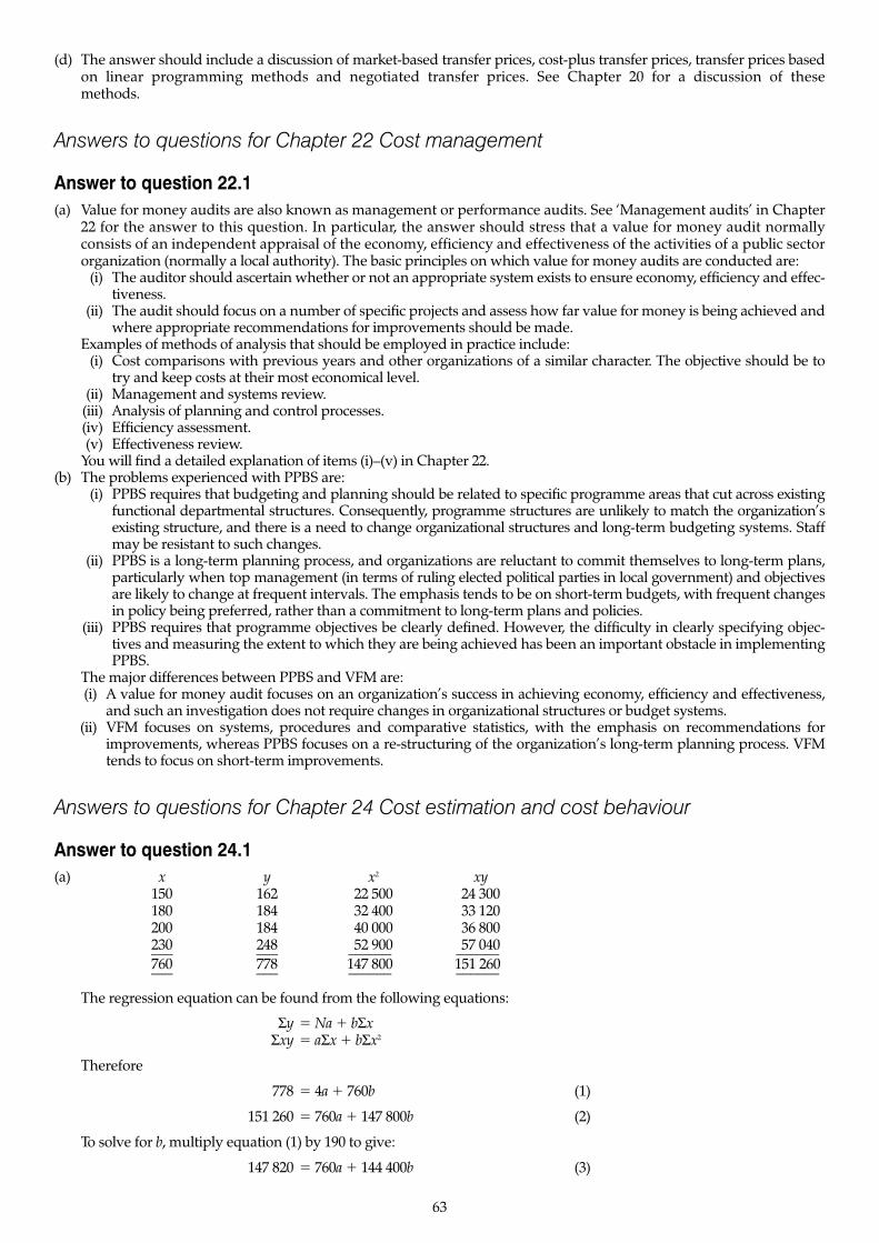
(d) The answer should include a discussion of market-based transfer prices, cost-plus transfer prices, transfer prices basedon linear programming methods and negotiated transfer prices. See Chapter 20 for a discussion of these methods.
Answers to questions for Chapter 22 Cost management
Answer to question 22.1(a) Value for money audits are also known as management or performance audits. See ‘Management audits’ in Chapter
22 for the answer to this question. In particular, the answer should stress that a value for money audit normallyconsists of an independent appraisal of the economy, efficiency and effectiveness of the activities of a public sectororganization (normally a local authority). The basic principles on which value for money audits are conducted are:
(i) The auditor should ascertain whether or not an appropriate system exists to ensure economy, efficiency and effec-tiveness.
(ii) The audit should focus on a number of specific projects and assess how far value for money is being achieved andwhere appropriate recommendations for improvements should be made.
Examples of methods of analysis that should be employed in practice include:(i) Cost comparisons with previous years and other organizations of a similar character. The objective should be to
try and keep costs at their most economical level.(ii) Management and systems review.
(iii) Analysis of planning and control processes.(iv) Efficiency assessment.(v) Effectiveness review.
You will find a detailed explanation of items (i)–(v) in Chapter 22.(b) The problems experienced with PPBS are:
(i) PPBS requires that budgeting and planning should be related to specific programme areas that cut across existingfunctional departmental structures. Consequently, programme structures are unlikely to match the organization’sexisting structure, and there is a need to change organizational structures and long-term budgeting systems. Staffmay be resistant to such changes.
(ii) PPBS is a long-term planning process, and organizations are reluctant to commit themselves to long-term plans,particularly when top management (in terms of ruling elected political parties in local government) and objectivesare likely to change at frequent intervals. The emphasis tends to be on short-term budgets, with frequent changesin policy being preferred, rather than a commitment to long-term plans and policies.
(iii) PPBS requires that programme objectives be clearly defined. However, the difficulty in clearly specifying objec-tives and measuring the extent to which they are being achieved has been an important obstacle in implementingPPBS.
The major differences between PPBS and VFM are:(i) A value for money audit focuses on an organization’s success in achieving economy, efficiency and effectiveness,
and such an investigation does not require changes in organizational structures or budget systems.(ii) VFM focuses on systems, procedures and comparative statistics, with the emphasis on recommendations for
improvements, whereas PPBS focuses on a re-structuring of the organization’s long-term planning process. VFMtends to focus on short-term improvements.
Answers to questions for Chapter 24 Cost estimation and cost behaviour
Answer to question 24.1(a) x y x2 xy
150 162 22 500 24 300180 184 32 400 33 120200 184 40 000 36 800230 248 52 900 57 040––– ––– –––––– ––––––760 778 147 800 151 260––– ––– –––––– ––––––
The regression equation can be found from the following equations:
Σy � Na � bΣxΣxy � aΣx � bΣx2
Therefore
778 � 4a � 760b (1)
151 260 � 760a � 147 800b (2)
To solve for b, multiply equation (1) by 190 to give:
147 820 � 760a � 144 400b (3)
63
Subtracting equation (3) from equation (2) gives:
3400b � 3440b = 1.012
Substituting for b in equation (1):
778 � 4a � 760 � 1.012a = 2.22
At the planned output level of 260 000 units the contribution is:
2.22 � 1.012 � 260 � 265.34 � £265 340(b) The 95% confidence limit is:
265.34 � 4.303 � 14.5 � 265.34 � 62.39Upper limit £327 730Lower limit £202 950
These are the limits within which we can be 95% certain the actual value of the contribution will be, given the assump-tions made.
(c) The advantages of using linear regression are:(i) It takes into account all available observations and yields more accurate results than the high–low method.
(ii) It determines the line of best fit mathematically, and is more accurate than visually determining the line of best fitusing graphical or scattergraph method.
(iii) It is a statistically valid method, and is preferable to subjective methods based on guesswork from past observa-tions.
For a discussion of the limitations of the technique see pages 964–68 in Chapter 24.
Answer to question 24.2(a) An estimate of the normal fixed and variable costs of production is required. The figures shown below therefore
exclude the winter heating costs of £10 000 in January and February.
Output x Total cost y xy x2
(000) (£000) (000) (000)January 9 105.2a 946.8 81February 14 172.0 2408.0 196March 11 125.4 1379.4 121April 8 96.0 768.0 64May 6 78.0 468.0 36June 12 140.4 1684.8 144–– ––––– –––––– –––
60 717.0 7655.0 642–– ––––– –––––– –––
Notea(9000 � £12.80) � £10 000The regression equation can be derived from the following two equations (see formulae (24.1) and (24.2) in Chapter 24)and solving for a and b:
Σy � Na � bΣx
Σxy � aΣx � bΣx2
Inserting the above computations into the formulae:
717 � 6a � 60b (1)
7655 � 60a � 642b (2)
Multiplying equation (1) by 10:
7170 � 60a � 600b (3)
Subtracting equation (3) from equation (2):
485 � 42b
b � 11.5476
Substituting the value for b in one of the above equations gives a value of 4.024 for a.Alternatively, the formula outlined in the question can be used:
64
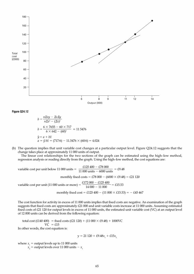
b �nΣxy � ΣxΣynΣx2 � (Σx)2
b �6 � 7655 � 60 � 717
= 11 54766 � 642 � (60)2
y- � a � bx-a � y- bx- � (717/6) � 11.5476 � (60/6) � 4.024
(b) The question implies that unit variable cost changes at a particular output level. Figure Q24.12 suggests that thechange takes place at approximately 11 000 units of output.
The linear cost relationships for the two sections of the graph can be estimated using the high–low method,regression analysis or reading directly from the graph. Using the high–low method, the cost equations are:
variable cost per unit below 11 000 units �£125 400 � £78 000
� £9.4811 000 units � 6000 units
monthly fixed costs � £78 000 � (6000 � £9.48) � £21 120
variable cost per unit (11 000 units or more) �£172 000 � £125 400
� £15.5314 000 � 11 000
monthly fixed cost � £125 400 � (11 000 � £15.53) � � £45 467
The cost function for activity in excess of 11 000 units implies that fixed costs are negative. An examination of the graphsuggests that fixed costs are approximately £21 000 and unit variable costs increase at 11 000 units. Assuming estimatedfixed costs of £21 120 for output levels in excess of 11 000 units, the estimated unit variable cost (VC) at an output levelof 12 000 units can be derived from the following equation:
total cost (£140 400) � fixed costs (£21 120) � (11 000 � £9.48) � 1000VCVC � £15
In other words, the cost equation is:
y � 21 120 � £9.48x1� £15x
2
where x1� output levels up to 11 000 units
x2� output levels over 11 000 units � x
1
65
6 8 9 11 12 14Output (000)
Totalcost(£000)
180
160
140
120
100
80
60
40
20
Figure Q24.12
(c) Observed EstimatedOutput costs Costsa difference
(000) (£000) (£000) (£000)January 9 105.2 106.44 (1.24)February 14 172.0 170.40 1.6March 11 125.4 125.40 0April 8 96.0 96.96 (0.96)May 6 78.0 78.00 0June 12 140.4 140.40 0
NoteaBased on cost equation 21 120 � 9.48x
1� 15x
2
(d) For the answer to this question see Chapter 24 (pages 964–68).
Answer to question 24.3(a) 5000 � 10 � 5000�0.3
� 10 � 0.07768� 0.7768
The average time taken to produce 1 unit is 0.7768 hours. Therefore 3884 hours (5000 � 0.7768) will be required toproduce 5000 units. It is assumed that 3884 hours per annum will be available for years 2 and 3. Hence the cumulativehours for years 1 and 2 will be 7768 (3884 � 2). It is therefore necessary to determine the number of units of output thatwill require 7768 hours.
Let yt� total number of hours. Then the average time (y) required to produce 1 unit of output is y
t/x, where x
represents the number of units of output. Applying the learning-curve formula:
y � axb
yt/x � axb
yt
� axb � 1
7768 � 10x0.7
x0.7 � 776.8x � 776.81/0.7
� 776.81.428 57
� 13 460
Thus the output for year 2 will be 8460 units (13 460 � 5000). For years 1–3 there are 11 652 hours (3884 � 3) available.Applying the above approach:
11 652 � l0x0.7
x0.7 � 1165.2x � 1165.21.428 57
� 24 020
Thus the output for year 3 will be 10 560 units (24 020 � 13 460).Instead of applying the above method, we can use a trial-and-error approach to determine the output for years 2
and 3. For year 2:
13 000 units � 10 � 13 000–0.3 � 0.5832 � 13 000 � 7581 hrs14 000 units � 10 � 14 000–0.3 � 0.5704 � 14 000 � 7986 hrs
By trial and error, the learning-curve formula is applied to output levels between 13 000 and 14 000 units until the timerequired is equal to 7768 hours.
NPV calculationsYears 1 2 3Output 5 000 8 460 10 560––––– ––––– ––––––
(£) (£) (£)Sales (� £42) 210 000 355 320 443 520––––––– ––––––– –––––––Less costs:
Labour (3884 � £6) 23 304 23 304 23 304Material (� £30) 150 000 253 800 316 800Overheads 25 000 25 000 25 000––––––– ––––––– –––––––Total costs 198 304 302 104 365 104–––––––– –––––––– ––––––––Net cash flows � 11 696 � 53 216 � 78 416
66
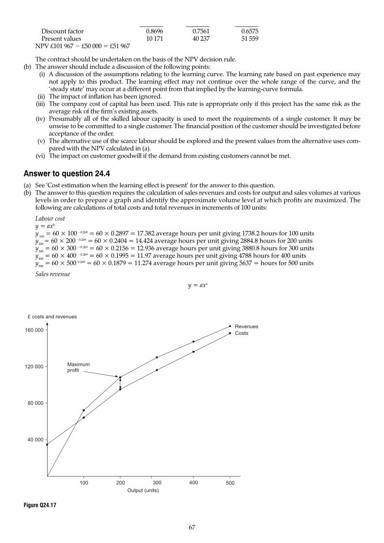
–––––––– –––––––– ––––––––Discount factor 0.8696 0.7561 0.6575Present values 10 171 40 237 51 559
NPV £101 967 � £50 000 � £51 967
The contract should be undertaken on the basis of the NPV decision rule.(b) The answer should include a discussion of the following points:
(i) A discussion of the assumptions relating to the learning curve. The learning rate based on past experience maynot apply to this product. The learning effect may not continue over the whole range of the curve, and the‘steady state’ may occur at a different point from that implied by the learning-curve formula.
(ii) The impact of inflation has been ignored.(iii) The company cost of capital has been used. This rate is appropriate only if this project has the same risk as the
average risk of the firm’s existing assets.(iv) Presumably all of the skilled labour capacity is used to meet the requirements of a single customer. It may be
unwise to be committed to a single customer. The financial position of the customer should be investigated beforeacceptance of the order.
(v) The alternative use of the scarce labour should be explored and the present values from the alternative uses com-pared with the NPV calculated in (a).
(vi) The impact on customer goodwill if the demand from existing customers cannot be met.
Answer to question 24.4(a) See ‘Cost estimation when the learning effect is present’ for the answer to this question.(b) The answer to this question requires the calculation of sales revenues and costs for output and sales volumes at various
levels in order to prepare a graph and identify the approximate volume level at which profits are maximized. Thefollowing are calculations of total costs and total revenues in increments of 100 units:
Labour costy = axb
y100
= 60 × 100 �0.269 = 60 × 0.2897 = 17.382 average hours per unit giving 1738.2 hours for 100 unitsy
200 = 60 × 200 �0.269 = 60 × 0.2404 = 14.424 average hours per unit giving 2884.8 hours for 200 units
y300
= 60 × 300 �0.269 = 60 × 0.2156 = 12.936 average hours per unit giving 3880.8 hours for 300 unitsy
400= 60 × 400 �0.269 = 60 × 0.1995 = 11.97 average hours per unit giving 4788 hours for 400 units
y500
= 60 × 500 0.269 = 60 × 0.1879 = 11.274 average hours per unit giving 5637 = hours for 500 units
Sales revenue
y = axn
67
100 200 300 400 500
120 000
160 000
80 000
40 000
£ costs and revenues
Maximumprofit
Revenues
Costs
Output (units)
Figure Q24.17
where y = average selling price for x unitsa = the selling price for the first unit of outputx = the number of units of output under considerationn = exponent function
£327.80 = £10 000 × 500n
£327.80/£10 000 = 500n
0.03278 = 500n
n = log 0.03278 / log 500 = �3.1479 / 6.2146 = �0.55y
100 = £10 000 × 100 �0.55 = £10 000 × 0.07943 = £794.30 selling price giving £79 430 for 100 units
y200
= £10 000 × 200 �0.55 = £10 000 × 0.05425 = £542.50 selling price giving £108 500 for 200 unitsy
300 = £10 000 × 300 �0.55 = £10 000 × 0.04341 = £434.10 selling price giving £130 233 for 300 units
y400
= £10 000 × 400 �0.55 = £10 000 × 0.03706 = £370.60 selling price giving £148 240 for 400 unitsy
500 = £10 000 × 500 �0.55 = £10 000 × 0.03278 = £327.80 selling price giving £163 900 for 500 units
Projected cost, revenues and profitsOutput Labour Labour Other variable Fixed Total Total Profit/(loss)(units) hours cost (£) costs (£) costs (£) cost (£) revenues (£) (£)
0 35 000 35 000 (35 000)100 1738.2 34 764 2 000 35 000 71 764 79 430 7 666200 2884.8 57 696 4 000 35 000 96 696 108 500 11 804300 3880.8 77 616 6 000 35 000 118 616 130 233 11 617400 4788.0 95 760 8 000 35 000 138 760 148 240 9 480500 5637.0 112 740 10 000 35 000 157 740 163 900 6 160
The above information is plotted on the graph shown in Figure Q24.17.
(c) It is apparent from the graph and the schedule shown in part (b) that profit maximizing output level is around an out-put level of 200 units but that profit is not very sensitive to output changes between 200 and 300 units.
Answers to questions for Chapter 25 Quantitative models for the planning and control ofstocks
Answer to question 25.1(a) (i) Continuous stocktaking refers to a situation where a sample of stores items are counted regularly on, say, a daily
basis. Sufficient items should be checked each day so that during a year all items are checked at least once. Thealternative system of stocktaking is a complete physical stockcount where all the stock items are counted at onepoint in time. Continuous stocktaking is preferable because production is not disrupted and any discrepanciesand losses are revealed earlier.
(ii) A perpetual inventory system is a stock recording system whereby the balance is shown for a stock item aftereach receipt or issue. In a non-computerized system the records are maintained on bin cards or stores ledgercards. A separate record is maintained for each item of materials in stores. Therefore the stock balance for eachstores item is available at any point in time.
(iii) For an explanation of ABC inventory analysis see ‘Control of stocks through classification’ in Chapter 25.(b) For the answer to this question you should refer to Chapter 25 (‘Relevant costs for quantitative models under
conditions of certainty’ and ‘Determining the economic order quantity’).(c) Normal control levels are the reorder level, minimum level, and maximum level.
Reorder level � maximum usage � maximum lead time� 800 kg � 14 days� 11 200 kg
Minimum level � re-order level � average usage in average lead time� 11 200 kg � (600 kg � 12 days)� 4000 kg
Maximum level � re-order level � EOQ – minimum usage in minimum lead time� 11 200 kg � 12 000 kg � (400 kg � 10 days)� 19 200 kg
68
Answer to question 25.2(a) Item A32: storage and ordering cost schedule
No. of orders per year 4 5 6 7 8 9 10 11 12Order size (boxes) 1250 1000 833 714 625 556 500 455 417Average stock (boxes) 625 500 417 357 313 278 250 228 208
(£) (£) (£) (£) (£) (£) (£) (£) (£)Storage costs(average stock x 25%
of £2) 312.5 250.0 208.5 178.5 156.5 139.0 125.0 114.0 104.0Ordering costs
(£12.5 per order) 50.0 62.5 75.0 87.5 100.0 112.5 125.0 137.5 150.0
Total cost £362.5 £312.5 £283.5 £266.0 £256.5 £251.5 £250.0 £251.5 £254.0
(b) The number of orders which should be placed in a year to minimize costs is 10.
(c) EOQ � � �2DO�H
where D = total demand for period, O � ordering cost per order, H � holding cost per unit.
(d) EOQ � � �2 � 5000 � 12.5�0.5
� 500 units
(e) The maximum saving that could be made if the authority process four orders per year would be:
£362.50 � £250� 31%
£362.50
(f) (i) Reducing the number of stock items by eliminating slow moving and obsolete stocks.(ii) Standardization of stock items thus reducing the total number of items in stock.
Answer to question 25.3(a) (i) EOQ � � �2DO�H
where D � annual demand, O � ordering cost per order, H � holding cost per unit. Therefore:
EOQ � � �2 � 48 000 � £0.60�10% � £10
� 240(ii) Number of orders required per year is:
annual requirements�
48 000� 200 orders per yearEOQ 240
(iii) Total cost � holding costing � ordering cost
�240 (£1)
�48 000 (£0.60)
2 240
� £240
(b) Usage per day � 133.33 (48 000/360 days)Number of days’ usage in closing stock � 3 (400/133.33)Lead time � 3 daysTherefore the next order should be placed immediately.
(c) Some problems when attempting to apply the EOQ formula are:(i) Inventory is not always used at a constant rate, and the constant usage assumption is implicit in the EOQ formula.
(ii) The EOQ formula requires estimates of (a) annual sales, (b) ordering costs, (c) purchase price per unit and (d) costof carrying inventories. These items may be extremely difficult to estimate in practice.
69

Answer to question 25.4(a) (i) The cost of sales expressed as a percentage of total sales is 100 � Gross Margin %. Product A � 58% (100 � 42%),
Product B � 54%, Product C � 63%.
Weekly cost of sales (£000s)Minimum Maximum
14/363 26 � 0.58 � 15.08 30 � 0.58 � 17.4011/175 130 � 0.54 � 70.20 160 � 0.55 � 86.4014/243 60 � 0.63 � 37.80 128 � 0.63 � 80.64
Weekly sales (units)Minimum Maximum
14/363 15.08/2.25 � 6702 17.40/2.25 � 773311/175 70.20/0.36 � 195 000 86.40/0.36 � 240 00014/243 37.80/0.87 � 43 448 80.64/0.87 � 92 690
(ii) Re-order level � Maximum usage � maximum lead time14/363 � 7733 � 2 � 15 466 units11/175 � 240 000 � 2 � 480 000 units14/243 � 92 690 � 2 � 185 380 units
(iii) Maximum stock control level� Re-order level � EOQ (Minimum usage in minimum lead time)14/363 � 15 466 � 25 000 � (6 702 � 2) � 27 062 units11/175 � 480 000 � 500 000 � (195 000 � 2) � 590 000 units14/243 � 185 380 � 250 000 � (43 448 � 2) � 348 484 units
(b) 1. Excessive stocks of item 14/363 are being held since stock exceeds the maximum stock level;2. Stock is below the re-order level for item 11/175 and there are no outstanding orders. An order should have been
raised;3. The order for item 14/243 has been placed too early since stock exceeds the re-order level.
Answer to question 25.5(a) EOQ � � �2DO�H
EOQ � � �2 � 50 000 � 100�0.40
� 5000(b) (£)
Savings in purchase price (50 000 � £0.02) � 1000Saving in ordering costa
DO�
DO = 50 000 � 100�
50 000 � 100� 500––– ––– ––––––––––– –––––––––––
Qd
Q 10 000 5000 ––––Total savings 1500––––
NoteaQ
drepresents quantity ordered to obtain discount and Q represents EOQ. The additional holding cost if the larger
quantity is purchased is calculated as follows:
(Qd
� Q)H�
(10 000 � 5000) � 0.40� £1000
2 2
As the total savings exceed the total cost increase, the company should take advantage of the quantity discount.
70
Answer to question 25.6(a) Annual material costs are £9m (30% 3 £30m) and conversion costs are £7.5m (25% 3 £30m).
Current stock levels are: (£)Raw materials (10% � £9m) 900 000Work in progress:
Materials element £1 350 000 (15% � £9m)Conversion cost 675 000 (15% � £7.5 m � 60%) 2 025 000–––––––––
Finished goods:Materials element £1 080 000 (12% � £900 000)Conversion cost 900 000 (12% � £7.5m) 1 980 000–––––––––
The stockholding costs for each category of stocks are as follows:
Existing RevisedRaw material stock: (£) (£)
Fixed holding andacquisition costs 100 000 20 000
Variable holding andacquisition costs 90 000 (10%) 12 600 (20% � £900 000 � £0.07)
Financial charges 180 000 (20%) 36 000 [20% � (20% � £900 000)]––––––– ––––––370 000 68 600––––––– ––––––
Work in progress:Fixed movement and
control costs 140 000 56 000 (40% � £140 000)Variable movement
and control costs 67 500 (5% � £1.35 m) 8 100 [£0.03 � (20% � £1.35m)]Financial charges 405 000 (20% � £2025 m) 81 000 [20% � (20% � £2.025m)]––––––– ––––––
612 500 145 100––––––– ––––––
Finished goods:Fixed holding and
control costs 180 000 72 000 (40% � £180 000)Variable holding
and control costs 39 600 (2% � £1.98m) 4 950 [0.01 � (25% � £1.98m)] Financial charges 396 000 (20% � £1.98m) 99 000 [20% � (25% � £1.98m)]––––––– ––––––
615 600 175 950––––––– ––––––
Summary of cost savingsExisting Revisedsituation situation Savings
(£) (£) (£)Raw material stock 370 000 68 600 301 400Work in progress 612 500 145 100 467 400Finished goods 615 600 175 950 439 650–––––––– ––––––– ––––––––
1 598 100 389 650 1 208 450–––––––– ––––––– ––––––––
(b) Possible reasons for the reduction in costs for each item of stock are as follows:Raw material stock
(i) Reduction in insurance and clerical costs(ii) Reduction in number of staff required
(iii) Savings arising from reduction in warehouse space(iv) Reduction in materials handling cost(v) Reduced financing costs
Work in progress(i) Reduction in losses arising from moving WIP from one department to another
(ii) Reduction in materials handling equipment and staff(iii) Savings or additional cash flows arising from reduced storage space(iv) Reduced financing costsFinished goods stock
(i) Reduction in insurance costs(ii) Savings arising from reduction in warehouse space and staff
(iii) Reduction in finished goods handling costs(iv) Reduced financing costs
(c) For just-in-time purchasing it is essential that reliable suppliers can be found who will deliver to match the company’sproduction demands. Any later deliveries may result in stockout costs. Suppliers may increase purchase costs tocompensate for synchronizing their delivery and production schedules to the JIT production requirements of Prodco.
71

Alternatively, savings might arise from negotiating large long-term contracts with fewer suppliers. Dealing with fewersuppliers should result in a significant reduction in administrative costs. The reduction in stocks should create excessstorage space which might be used to increase production capacity. Alternatively, it may be possible to sub-let thespace.
The move to a cell layout should enable the company to respond quickly to changes in sales demand or to meetspecial orders. Thus additional sales might be generated. Additional training costs will be necessary to train theworkers to operate different types of machines and carry out routine maintenance. Set-up costs may increase as thecompany moves from producing large batches using batch production techniques to producing small or single unitbatches using flow production techniques.
JIT manufacturing should reduce finished goods stocks since the aim is to produce the required quantities at theprecise time they are required. This should result in improved customer goodwill if production is more sensitive tomeeting customer delivery requirements. The reduction in finished goods stock requirements will create additionalstorage space which might generate additional rental income from sub-letting.
Answer to question 25.7(a) The re-order point based on the expected usage and lead time is calculated as follows:
ExpectedTotal demand Joint value
during lead time probability (usage)75 000 (15 � 5000) 0.1 7 500
105 000 (15 � 7000) 0.1 10 500100 000 (20 � 5000) 0.25 25 000140 000 (20 � 7000) 0.25 35 000125 000 (25 � 5000) 0.15 18 750175 000 (25 � 7000) 0.15 26 250–––- ––––––
1.00 123 000–––- ––––––
With a re-order level of 150 000 units, the safety stock (buffer stock) is 27 000 units (150 000 – 123 000).(b) The probability of a stockout (i.e. demand in excess of 150 000 units) is 0.15.
(c) EOQ � � �2 � (6000 � 240) � 1000� � 138 564 units0.15
Note that the expected daily demand of 6000 units is calculated as follows:
(0.5 � 5000) � (0.5 � 7000)
The average number of orders per annum is:
6000 � 240� 10.39
138 564
The expected annual stockouts in units per annum is:
0.15 � (175 000 � 150 000) � 10.39 � 38 962 units
(d) The additional annual holding cost if the re-order level is increased to 175 000 units is £3750 (25 000 � £0.15).At a re-order level of 150 000 units, the expected value of the stockouts per annum is 38 962 units.Therefore the increase in stock is justified where the stockout cost per unit is greater than 9.6 pence (£3750/38 962
units).(e) Many companies are now giving increasing attention to reducing stocks to a minimum by adopting just-in-time (JIT
purchasing and production techniques. For a description of JIT techniques you should refer to Chapter 22. The maindisadvantage of JIT purchasing is that a successful JIT philosophy depends on finding suppliers who can provide areliable delivery service at frequent intervals. With the absence of stocks, the system is dependent on a reliable servicebeing maintained with no delay in deliveries. JIT companies therefore become very dependent upon the reliability ofthe supplier, and any failure by the latter to meet delivery schedules could have a serious impact on a wholeproduction process.
72
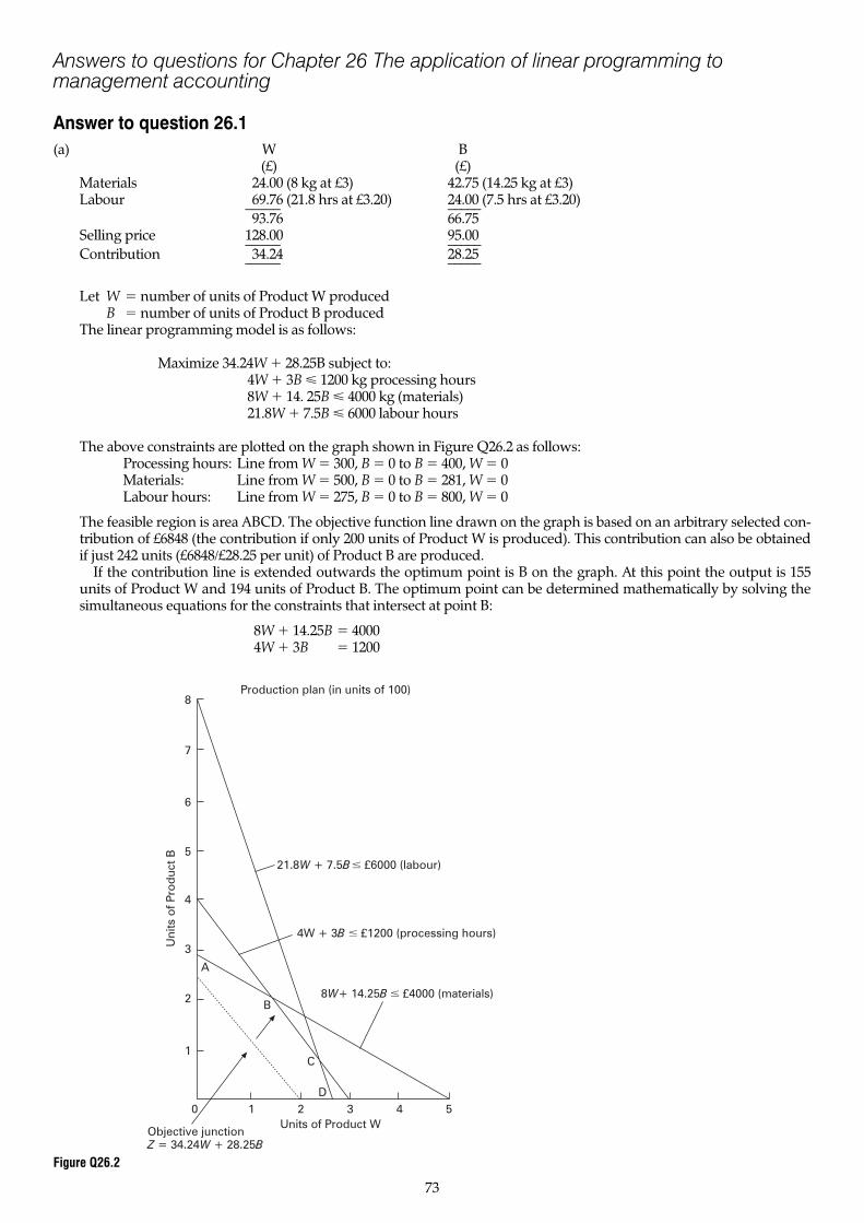
Answers to questions for Chapter 26 The application of linear programming tomanagement accounting
Answer to question 26.1(a) W B
(£) (£)Materials 24.00 (8 kg at £3) 42.75 (14.25 kg at £3)Labour 69.76 (21.8 hrs at £3.20) 24.00 (7.5 hrs at £3.20)––––– –––––
93.76 66.75Selling price 128.00 95.00––––– –––––Contribution 34.24 28.25––––– –––––
Let W � number of units of Product W producedB � number of units of Product B produced
The linear programming model is as follows:
Maximize 34.24W � 28.25B subject to:4W � 3B � 1200 kg processing hours8W � 14. 25B � 4000 kg (materials)21.8W � 7.5B � 6000 labour hours
The above constraints are plotted on the graph shown in Figure Q26.2 as follows:Processing hours: Line from W � 300, B � 0 to B � 400, W � 0Materials: Line from W � 500, B � 0 to B � 281, W � 0Labour hours: Line from W � 275, B � 0 to B � 800, W � 0
The feasible region is area ABCD. The objective function line drawn on the graph is based on an arbitrary selected con-tribution of £6848 (the contribution if only 200 units of Product W is produced). This contribution can also be obtainedif just 242 units (£6848/£28.25 per unit) of Product B are produced.
If the contribution line is extended outwards the optimum point is B on the graph. At this point the output is 155units of Product W and 194 units of Product B. The optimum point can be determined mathematically by solving thesimultaneous equations for the constraints that intersect at point B:
8W � 14.25B � 40004W � 3B � 1200
73
1 2 3 4 5Units of Product W
0
8
7
6
5
4
3
2
1
Uni
ts o
f Pro
duc
t B
Production plan (in units of 100)
21.8W + 7.5B 6000 (labour) £
4W + 3 £1200 (processing hours)B
8W B+ 14.25 £4000 (materials)
A
B
C
D
Objective junctionZ = 34.24 + 28.25W B
Figure Q26.2

The values of W and B when the above equations are solved are 155 for W and 194 for B. This will yield a total contri-bution of £10 788.
(b) The answer should also include the following points:(i) Few production resources are entirely fixed in the short term apart from machine capacity. Steps can often be
taken to remove the constraints, such as obtaining materials from alternative sources or increasing machinecapacity by working longer hours;
(ii) A narrow focus has been adopted. Consideration should be given to increasing selling prices to the point wheredemand is equal to maximum output arising from the current production considerations;
(iii) The approach ignores marketing considerations. Long-term profits might be maximized by concentrating pro-duction on one of the products to capture a large market share so that market dominance can be established andmore substantial profits obtained;
(iv) Linear programming tends to focus on the short term whereas the emphasis should be on maximizing long-runprofits.
Answer to question 26.2(a) The calculations of the product contributions are:
Private Commercial(£) (£)
Selling price 2400 3200Materiala (200) (250)Direct labour (90) (108)Variable production costs (250) (312)–––– ––––Contribution 1860 2530–––– ––––
NoteaThe contribution should reflect the additional cash flow contribution from selling an extra roll. The material costsgiven in the question represent sunk costs and are not relevant costs to be included in the contribution calculation. Therelevant cost of materials is the lost sales value of £1 per lb of wool or nylon (that is, 200 lb at £1 for private use and 250� £1 for commercial use).
Let X � number of rolls of private useLet Y � number of rolls of commercial use
Then the linear programming formulation is:
Maximize 1860X � 2530Y subject to40X � 200Y � 24 000 (wool constraint)
160X � 50Y � 25 000 (nylon constraint)30X � 36Y � 6600 (machine time constraint)
X 0Y 0
The above constraints are plotted on the graph in Figure Q26.6 as follows:
74
Private ( )X
A
B
CWool 40 + 200 24 000
XY
3002001500
100 D
Nylon 160X
Y+
5025 000
Machinery 30X
Y
+ 36
6600
Commercial (Y)
200
150
100
80
50
Objective function line Z = £186 000(arbitrarily chosen contribution figure)
Figure Q26.6
Wool constraint: line from X � 600, Y � 0 to Y � 120, X � 0Nylon constraint: line from X � 156.25, Y � 0 to Y � 500, X � 0Capacity constraint: line from X � 220, Y � 0 to Y� 183.33, X � 0
At the optimum point (B in the graph) the output mix is 100 rolls for private use and 100 rolls for business use. Theoptimum point can be determined mathematically by solving the simultaneous equations for the constraints thatintersect at point B:
30X � 36Y � 6 60040X � 200Y � 24 000
The values of X and Y when the above equations are solved are 100 for � and 100 for Y. The optimum outputrequires 24 000 lb of wool to be used but only 21 000 lb of nylon. Therefore 4000 lb of nylon will be sold off at £1 per lb.The total contribution for the quarter is:
(£)Rolls for private use (100 � £1600) 160 000Rolls for commercial use (100 � £1980) 198 000Loss on sale of nylon [4000 � (£2 � £1)] (4 000)
–––––––354 000–––––––
The above calculation reflects the contribution that would be shown in the accounting statements using accrualaccounting. Alternatively, the contribution can be calculated using the relevant cost approach. This alternative contri-bution calculation reflects the additional contribution over and above that which would be obtained from the alterna-tive use of materials.
(b) If the variable costs increase then the contribution will decline by £110 for private sales and £40 for commercial sales.The revised contribution will be:
Z � 1750X � 2490Y
You will find that the gradient of the revised objective function line is such that the optimal point remains unchanged,and therefore the optimal output remains the same.
(c) The scarce resources are machine hours and wool. This is because these two constraints intersect at the optimum pointB. If an additional machine hour were obtained, the binding constraints would become:
Wool 40X � 200Y � 24 000Machine capacity 30X � 36Y � 6 601
The value of X and Y when the above equations are solved are 100.04 for X and 99.99 for Y. Therefore X increases by0.04 rolls and Y decreases by 0.01 rolls, and the change in contribution will be as follows:
(£)Increase in contribution of X (0.04 � £1860) 74.40Decrease in contribution of Y (0.01 � £2530) 25.30–––––Increase in contribution 49.10–––––
If an additional lb of wool were obtained, the optimal solution would change such that X should be decreased by 0.01rolls and Y increased by 0.01 rolls. Contribution would increase by £6.70.
(d) The answer should stress the advantages of valuing variances at opportunity cost (i.e. relevant cost) rather thanacquisition cost. For a detailed explanation of the opportunity cost approach see ‘Variance analysis and theopportunity cost of scarce resources’ in Chapter 19. The answer should also include a discussion of the limitationplaced on opportunity costs because of the limitations of linear programming. The limitations include:
(i) Linearity is assumed. In practice, stepped fixed costs might exist or resources might not be used at a constant ratethroughout the entire output range. Selling prices might have to be reduced to increase volume.
(ii) The output of the model is dependent on the accuracy of the estimates used. In practice, it is difficult to segregatecosts into their fixed and variable elements.
(iii) The objective function must be quantifiable and not of a qualitative nature.(iv) Constraints are unlikely to be as completely fixed and precise as implied in the mathematical model. Some con-
straints can be removed at an additional cost.
75

Answer to question 26.3(a) It is assumed that sales demand for Alpha is restricted to 200 units.
Maximize 400x1� 200x
2� 300x
3
Subject to: 2x1� 3x
2� 2.5x
3� 1920 (Process 1)
3x1� 2x
2� 2x
3� 2200 (Process 2)
x1
� 200 (Alpha sales)x
1, x
2, x
3 0 (Minimum sales constraint)
(b) x1
x2
x3
x4
� 1920 �2 �3 �2.5x
5� 2200 �3 �2 �2
x6
� 200 �1 �0 �0Z � 0 �400 �200 �300
Slack variables represent unused resources and unused sales potential.(c) There are several ways of formulating the tableau for a linear programming model. The tableau given in the question
can be reproduced as follows:
x3
x4
x6
x2
506.7 �0.83 �0.33 �0.67x
5586.7 �0.33 �0.67 �1.67
x1
200 �0 �0 �1Z 181 333.3 �66.67 �66.67 266.7
In Chapter 26 the approach adopted was to formulate the first tableau with positive contribution signs and negativesigns for the slack variable equations. The optimal solution occurs when the signs in the contribution row are allnegative. The opposite procedure has been applied with the tableau presented in the question. Therefore the signshave been reversed in the above tableau in order to ensure that it is in the same format as that presented in Chapter 26.Note that an entry of 1 in the tableau presented in the question signifies the product or slack variable that is to beentered in each row of the above tableau.
The total contribution is £181 333.3, consisting of 200 units of Alpha and 506.7 units of Beta. Process 1 (x4) is fully
utilized, but 586.7 hours (x5) of Process 2 are unused. There is no unused sales demand for Alpha. The Z row
(contribution row) indicates the shadow prices. The shadow price of £66.67 for Gamma (x3) indicates that contribution
will decline by £66.67 for each unit of Gamma produced. The shadow price of £66.67 for Process 1 (x4) indicates that for
each additional hour of Process 1 contribution would increase by £66.67. This would be achieved by increasing outputof Beta by 0.33 units, and the effect of this would be to reduce Process 2 capacity by 0.67 hrs. The shadow price of£266.7 for Alpha (i.e. the slack variable) implies that for every Alpha sale above 200 units contribution would increaseby £266.7. In order to produce one unit of Alpha, output of Beta will be reduced by 0.67 units, thus releasing the 2 hrs(0.67 � 3 hrs) required for Alpha in Process 1. This substitution process will result in a decline of 1.67 hrs in Process 2.
(d) The optimal responses are indicated in the final tableau:(i) Increase output of Beta by 6.66 units (20 � 0.33) at a contribution of £200 per unit. Therefore total contribution
will increase by £1332 to £182 665.7. Alternatively, the change in contribution can be obtained by multiplying the20 additional hours by the shadow price of £66.67.
(ii) This will increase total contribution by £2667 (10 units � £266.7 shadow price). In order to produce an additionalunit of Alpha, the output of Beta must be reduced by 6.7 units (10 � 0.67). This will release 20 hours (6.7 units � 3hrs for Beta) in Process 1, which are required to produce the 10 units of Alpha (10 � 2 hrs). This substitutionprocess requires 16.7 Process 2 hours, and results in a £2667 increase in total contribution (10 units of Alpha at £400per unit less 6.7 units of Beta at £200 per unit).
(iii) Total contribution will be reduced by £666.7 (10 units � £66.7 shadow price). In order to obtain the hours requiredto produce Gamma in Process 1, the output of Beta must be reduced by 8.3 units (0.83 � 10 units required forGamma). This will release 25 hrs (8.3 � 3 hrs) in Process 1, which is required to produce 10 units (10 � 2.5 hrs) ofGamma. This substitution process will reduce Process 2 unused capacity by 3.3 hrs and reduce total contributionby £666.7 (10 units of Gamma at £100 per unit less 8.3 units of Beta at £200 per unit).
Answer to question 26.4(a) Let x
1� proportion of project A undertaken
x2� proportion of project B undertaken
x3� proportion of project C undertaken
x4� proportion of project D undertaken
x5� proportion of project E undertaken
x6� cash unused at time 1 and carried forward to time 2
x7� cash unused at time 2 and carried forward to time 3
76
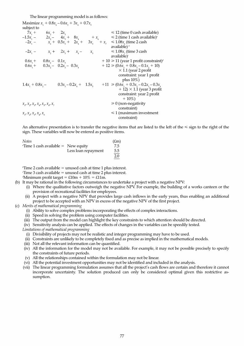
The linear programming model is as follows:Maximize x
1� 0.8x
2– 0.6x
3� 3x
4� 0.7x
5
subject to7x
1� 6x
2� 2x
3� 12 (time 0 cash available)
–1.5x1
– 2x2– 4x
3� 8x
4� x
6� 2 (time 1 cash available)a
–2x1
– x2� 0.5x
3� 2x
4� 3x
5� x
7� 1.08x
6(time 2 cash
available) b
–2x1
– x2+ 2x
3+ x
4– x
5� 1.08x
7(time 3 cash
available)c
0.6x1� 0.8x
2– 0.1x
3� 10 11 (year 1 profit constraint)d
0.6x1� 0.3x
2– 0.2x
3– 0.3x
4� 12 (0.6x
1� 0.8x
2– 0.1x
3� 10)
� 1.1 (year 2 profitconstraint: year 1 profit
plus 10%)1.4x
1� 0.8x
2– 0.3x
3– 0.2x
4� 1.5x
5�11 (0.6x
1� 0.3x
2– 0.2x
3– 0.3x
4
� 12) � 1.1 (year 3 profitconstraint: year 2 profit
� 10%)x
1, x
2, x
3, x
4, x
5, x
6, x
7 0 (non-negativity
constraint)x
1, x
2, x
3, x
4, x
5� 1 (maximum investment
constraint)
An alternative presentation is to transfer the negative items that are listed to the left of the � sign to the right of thesign. These variables will now be entered as positive items.
Notes (£m)aTime 1 cash available � New equity 7.5
Less loan repayment 5.5–––2.0–––
bTime 2 cash available � unused cash at time 1 plus interest.cTime 3 cash available � unused cash at time 2 plus interest.dMinimum profit target � £10m � 10% � £11m.
(b) It may be rational in the following circumstances to undertake a project with a negative NPV:(i) Where the qualitative factors outweigh the negative NPV. For example, the building of a works canteen or the
provision of recreational facilities for employees.(ii) A project with a negative NPV that provides large cash inflows in the early years, thus enabling an additional
project to be accepted with an NPV in excess of the negative NPV of the first project.(c) Merits of mathematical programming
(i) Ability to solve complex problems incorporating the effects of complex interactions.(ii) Speed in solving the problem using computer facilities.
(iii) The output from the model can highlight the key constraints to which attention should be directed.(iv) Sensitivity analysis can be applied. The effects of changes in the variables can be speedily tested.
Limitations of mathematical programming(i) Divisibility of projects may not be realistic and integer programming may have to be used.
(ii) Constraints are unlikely to be completely fixed and as precise as implied in the mathematical models.(iii) Not all the relevant information can be quantified.(iv) All the information for the model may not be available. For example, it may not be possible precisely to specify
the constraints of future periods.(v) All the relationships contained within the formulation may not be linear.
(vi) All the potential investment opportunities may not be identified and included in the analysis.(vii) The linear programming formulation assumes that all the project’s cash flows are certain and therefore it cannot
incorporate uncertainty. The solution produced can only be considered optimal given this restrictive as-sumption.
77
Related Documents