Drug Supply Modeling Software: User Manual

Drug Supply Modeling Software: User Manual

Vladimir Anisimov, Valerii Fedorov, Richard Heiberger, Sourish Saha and Mark Kothapalli

GSK DDS Technical Report 2010-01

May 2010

This paper was reviewed and recommended for publication by

Professor William F. Rosenberger

Department of Statistics, George Mason University

Fairfax, VA, USA

Professor Christian Ritter

Ritter and Danielson Consulting sprl, Brussels, Belgium

Universite Catholique de Louvain, Louvain-la-Neuve, Belgium

Linda Danielson

Vice-President, Biostatistical Services at IDDI

Louvain-la-Neuve, Belgium

Copyright © 2010 by GlaxoSmithKline Pharmaceuticals

Drug Development Sciences

GlaxoSmithKline Pharmaceuticals

1250 South Collegeville Road, PO Box 5089

Collegeville, PA 19426-0989, USA

and

New Frontiers Science Park (South)

Third Avenue

Harlow, Essex, CM19 5AW, UK

Drug Supply Modeling Software: User Manual

Vladimir Anisimov, Valerii Fedorov, Richard Heiberger, Sourish Saha and Mark Kothapalli

Research Statistics Unit, Drug Development Sciences

GlaxoSmithKline Pharmaceuticals

ABSTRACT

The design of multicentre clinical studies consists of several interconnected stages including patient re-

cruitment prediction, choosing a randomization scheme and a statistical model for analyzing patient

responses, and drug supply planning. The Research Statistics Unit (RSU) at GlaxoSmithKline (GSK)

has developed a risk-based supply modeling tool using statistical principles. The tool predicts drug sup-

ply needed to cover patient’s demand in a single study with a given risk of running out of stock for a

patient. In order to support Clinical Trials Supply and Global Supplies Operations teams at GSK, the

RSU created a user-friendly RExcel interface embedding the risk-based supply modeling tool into the

Excel environment. This manual discusses screenshots to guide the user through using the interface.

1. Introduction

The design of multicentre clinical studies consists of several interconnected stages including patient re-

cruitment planning, choosing a randomization scheme, the statistical model for analyzing patient re-

sponses, and predicting the drug supply required to satisfy patient demand during the recruitment stage.

The uncertainties in recruitment and randomization substantially affect the drug supply stage. The drug

supply chain process is rather costly and therefore it is essential to use statistical tools to minimize drug

supply costs.

Our approach, based on stochastic modeling, allows us to build predictive bounds for the number of

patients on different treatment arms in different regions, to predict critical levels of drug supply required

to satisfy patient demand, and to evaluate the risk (probability) of running out of stock for a patient.

Currently the tool enhanced by RExcel Interface is widely used by clinical teams and has enabled sub-

stantial benefits in GSK R&D. In November 2009 the members of GSK’s R&D Supply Chain Team

won the European Supply Chain Excellence Award for Innovation, where the organizers made a specific

reference to the crucial role of the “risk-based prediction modelling tool” within GSK’s overall proposal,

4

recognizing the innovative way to address the problem of supply overages and the development and use

of a mathematical model at the project level to provide an innovative solution.

Our risk-based approach to drug supply prediction for a single study uses the notion of an acceptable risk

of a stock-out [Anisimov (2009b)]. An acceptable risk δ means that with probability 1 − δ all patients

in a particular study will receive the assigned treatment at the time of randomization. Correspondingly,

with probability δ in a particular study, at the time of randomization the assigned treatment assignment

may not be available for one of the patients and these patients will therefore be excluded from the study

protocol. Note that for typical scenarios, the probability of supply shortage for more than one patient

has magnitude much less than δ. Thus, for a typical study with 500 patients, risk 5% means that across

similar studies only one patient out of (500/0.05)=10,000 may be “out of stock”. Another way of looking

at this is: for 100 similar studies of 500 patients each, we risk losing one patient in each of 5 studies, but

in the other 95 studies all patients will receive the correct treatment assignments. Therefore, in general

it is not reasonable to use risk less than 5%. This approach is similar to what is used at the statistical

analysis stage: take a decision, based on patient responses and with a given probability of risk, on the

tested drug.

There are a few input parameters in the tool considered as basic, and several other secondary parameters

which in the current version of RExcel Interface are set by default, but can be changed for any specific

scenario. For each Scenario we have the following primary parameters in Table 1.

The description of the Scenario can be expanded to show additional details about the following secondary

parameters - distribution of centres between depots, initial period, re-supply interval, delivery time to

depots, intervals for prediction, delivery time to local sites, coefficient of variation in recruitment rates,

treatment proportions within randomization block. The tool covers two randomization schemes: Stratified

by centre and Unstratified (central). It accounts for the variation in patient recruitment between different

regions/depots, for the uncertainties caused by randomization scheme, and for specific logistics of re-

supply. In particular, it allows prediction of the upper bounds for the number of randomized patients

and supply demand in different regions for different time periods, estimation of the probabilities and the

number of various critical events in the regions, and selection of the amount of the initial shipment in

different regional depots.

The current technique of calculations is based on some approximations by the number of patients and

the number of centres (for Stratified by centre randomization). Therefore, to get practically relevant

results, the total number of patients should be at least 20 and in each depot the number of patients on

average should be at least 5. In the case of Stratified by centre randomization, the number of centres in

5

Table 1. Primary input parameters which define the Scenarios.

Number of Patients Sample size, total number of patients to be recruited (should be at

least 20)

Number of Centres Potentially available number of centers (must not be smaller than num-

ber of depots)

Number of Treatments Total number of treatments (must be at least 1)

Number of Depots Total number of regions or depots (must be greater than or equal to

number of centres)

Number of Dispenses Total number of dispenses (must be at least 1)

Risk Level Probability that in a study for not more than one patient a right

treatment is not available (should not be more than 0.5, recommended

range is [0.05,0.25])

Recruitment Duration Time available for recruitment (must be at least 1 day)

Treatment Duration Time required for enrolment and treatment (must be at least 1 day)

each depot should be at least 5. Furthermore, the recommended range for risk level is between 0.05 and

0.25. However, for studies with some “rare” diseases, if the team would like to substantially decrease the

potential opportunity of “running out of stock” and the cost of drug is not so important, the level of risk

can be set at lower level, e.g. 0.01. The tool does not encompass commonly observed supply challenges

such as batch shipment, import licenses, shelf-life, and production bottlenecks.

To facilitate the use of the Drug Supply Modeling tool and to make it more convenient for clinical

teams, the RSU has developed a user-friendly RExcel interface. RExcel [Baier and Neuwirth (2007),

Neuwirth et al. (2009)] integrates the powerful statistical and graphical functions in R [R (2009)] into

the familiar user interface of Excel [Microsoft (2007)]. Data can be exchanged between Excel and R.

The user can use R functions in Excel cell formulas, effectively controlling R calculations from Excel’s

automatic recalculation mechanism. By connecting R data frames and Excel data lists, it allows the

creation of a stand-alone RExcel workbook which hides R almost completely from the user and uses

Excel as the main interface to R.

In this technical report, the focus is on using the software implementing the statistical methodology out-

lined in [Anisimov and Fedorov (2005)]–[Anisimov (2010)]. Section 2 illustrates the interaction between

the user and the individual worksheets in the workbook. We provide concluding remarks in Section 3. In

the Appendix, we describe the R package and give detailed instructions on installation.

6

2. RExcel Interface

This section is an illustration of a modeling session for a clinical trial. We show the complete interaction

between the user and the interface program. We specify several Scenarios, defined by values of model

parameters such as number of patients and number of centres, to the program. We show the calculation

of the anticipated overages for each scenario with the MultiScenario worksheet of the Excel workbook

(Figures 1–5). We show the calculation of the sensitivity of the analysis with several additional worksheets

in the workbook in Figures 6–16. There are ten scenarios displayed in Figure 1. These have been chosen

to reflect the experience of recent GSK trials.

Figure 1. The MultiScenario worksheet allows computation of overages for up to ten

different scenarios (as specified in cell B2) based on two randomization types, “Stratified

by centre” and “Unstratified”. The randomization types are described in Section A.3.

The Worksheet opens with the primary parameters of the sample scenarios grayed out

in Cells B5:K12. These are the cells that will be used to specify the primary parameters

for the trial currently under design. When a non-zero value is placed in cell B2, the

scenario parameters appear dark (as in Figure 2).

7

Figure 2. We set cell B2 to 10. The button Calculate and Plot Overages in cell D13 is

pressed to initiate the overage calculations. The calculated overages for all scenarios are

displayed in cells B14:K15 in Figure 3 and plotted in Figure 4.

Figure 3. The overages calculated in Figure 2 are displayed in cells B14 through K15

and plotted in Figure 4.

8

a. Initial plot from Figure 2. b. After clicking the Identify Scenario button.

c. After clicking point 9 in Figure 4b.

Figure 4. Plot of predicted overages calculated in Figure 2 by the “Stratified by centre”

and “Unstratified” randomization schemes. As seen in this example, and supported by

theoretical results [Anisimov (2009b), Anisimov (2009c)], the overages from the “Strati-

fied by centre” scheme are always smaller than the ones from the “Unstratified” scheme.

Let us investigate Scenario 9 further by looking at, and possibly changing, its secondary parameters.

Press the button Identify Scenario in Figure 2 to show the selection cross-hairs in the plot (Figure 4b).

Click on a point (in this example, the point associated with Scenario 9) to get Figure 5. After clicking,

the dot for Scenario 9 is enlarged in the same color (Figure 4c).

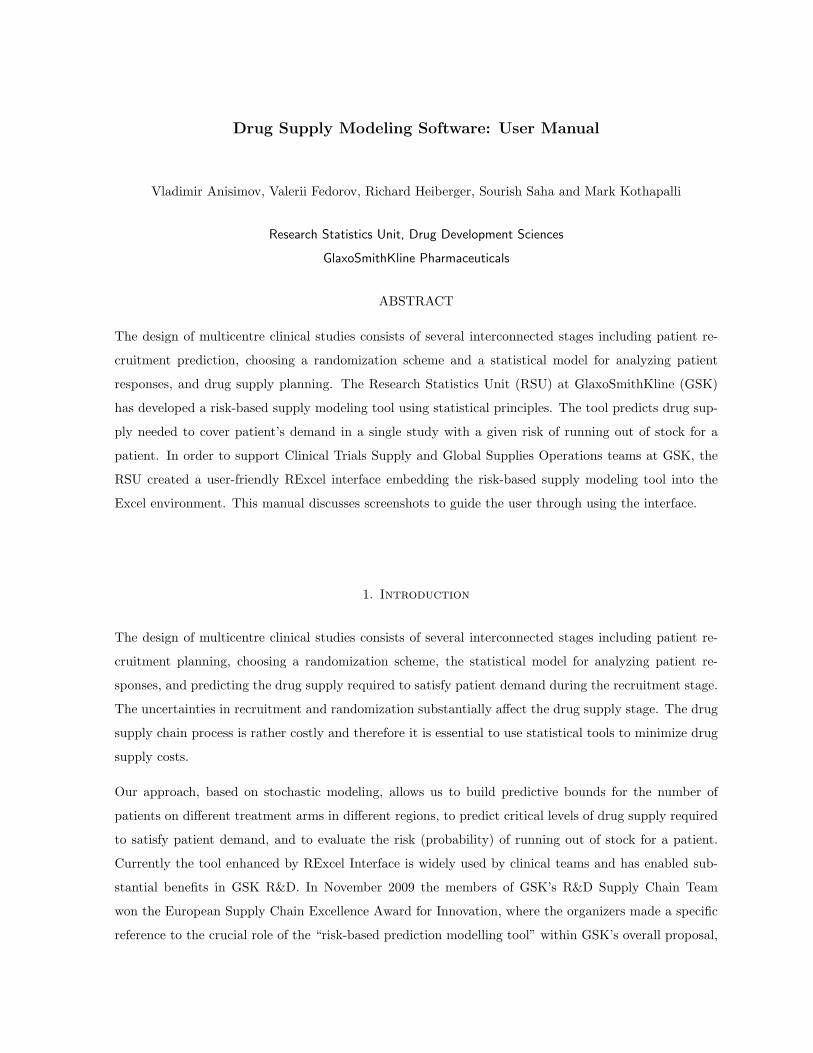
9

Figure 5. After clicking point 9 in Figure 4, the input parameters and the overage

values for Scenario 9 are highlighted in a lighter shade of the color displayed in the

column header. In addition, the secondary parameters for the highlighted scenario are

available for display and/or changing in Figure 6.

Figure 6. The AdvScenario worksheet allows the user to change the values of the

secondary parameters for the selected scenario as displayed in cell B1. The Show Default

button displays the default parameter values for the selected scenario. We show the

changes in Figure 7.

10

Figure 7. The user can change the secondary parameter values displayed in Figure 6

and then click on the button Save Edited values of Secondary Parameters. In this example,

we illustrate changing the distribution of centres for Depots 1 and 10. In Figure 6 we

had values 74 and 8; in this figure we have values 4 and 78. The changed secondary

parameters will be used after the user clicks on button Save Edited values of Secondary

Parameters and button Calculate and Plot Overages (full set from MultiScenario Tab)

.

The parameters in rows 12:15 are depot-related. The parameters in rows 17 and 19 are trial-related.

The parameter in row 23 is treatment-related. The new overage values calculated using these changed

secondary parameters are displayed in cells B26 and B27 of the AdvScenario worksheet. The cells B14:K15

in the Multiscenario worksheet and the graph in Figure 4a are also updated.

The button Show Current values of Secondary Parameters displays the edited values of the secondary

parameters while the button Reset Secondary Parameters in Excel and R to Default values sets the secondary

parameters back to their default values.

11

Figure 8. The Sensitivity worksheet is used to perform sensitivity analysis based on

the primary parameters for the selected scenario displayed in cell B1. By default the

minimum and maximum values for each parameter are set to their input values. In

Figure 9 we change some of the minimum and maximum values and run the Sensitivity

Analysis.

Figure 9. In this figure we change the minimum and maximum values for the number

of patients, centres, treatments, depots and dispenses. Then click the Calculate & Plot

Overages for All Active Scenarios button followed by Identify point in current Scenario

button.

12

Figure 10. The top panel shows the Sensitivity plot consisting of a colored dot indicat-

ing the overages for the initial values in column B of Figure 9, and open circles indicating

the overages for the set of scenarios at the 2k points specified by the minimum and max-

imum values in columns C and D of Figure 9. The bottom panel shows the Sensitivity

worksheet containing the parameter values corresponding to the scenario which the user

clicked in the top panel. In this example, we change the minimum and maximum values

for the number of patients, centres, treatments, depots and dispenses, hence k = 5 and

we see 32 open circles. In the top panel we clicked on one point. It turned green and

placed the parameter values corresponding to its scenario in column E of the bottom

panel.

13

Figure 11. The Variation worksheet is used to perform sensitivity analysis based on

both primary and secondary parameters. The user can provide minimum and maximum

values for the primary and secondary parameters. The button Show Default values of

Secondary Parameters displays the current secondary parameter values with their default

minimum and maximum values. The user can change these minimum and maximum

values of the secondary parameter values and then click on the button Save Edited values

of Secondary Parameters.

Figure 12. Upon clicking the button Calculate Overages, the overages, means, standard

deviations, and lower and upper 95% confidence boundaries of the overages are displayed

in cells B32:F33.

14

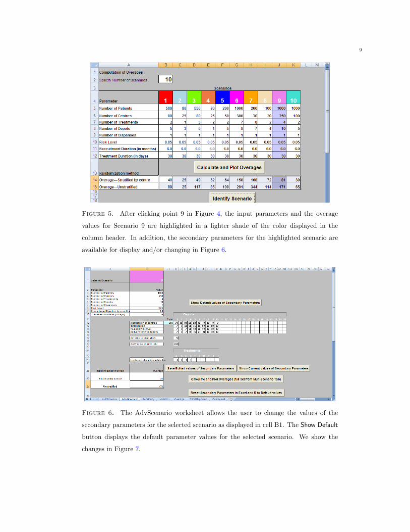
Figure 13. The Overage worksheet displays information about anticipated overages

and total number of packs for each treatment for the single scenario as specified on this

worksheet (the Overage worksheet does not inherit parameter values from the Multi-

Scenario worksheet). The Overage worksheet can calculate overages with or without

preloading (shipments of drugs prior to enrolment of any patients) of sites. The other

worksheets in this workbook assume no preloading. Clicking on the button Initial Ship-

ment takes the user to the InitialShipment worksheet as shown in Figure 14.

Figure 14. This figure is generated when the user clicks on the button Initial Shipment

in Figure 13. In this example, we specified two treatments and five depots in Figure 13.

The highlighted cells show the upper bound on the number of packets for each treatment

and depot combination for the “Unstratified” randomization scheme.

15

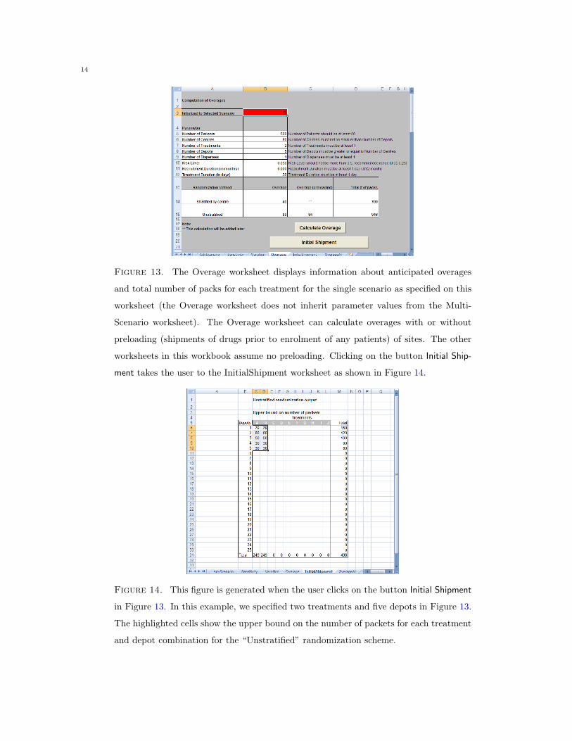
Figure 15. The OverageAll worksheet is used to generate six different plots of overages

by the following variables: number of patients, number of centres, number of treatments,

number of depots, number of dispenses, and risk level. After specifying the minimum,

maximum, and increment values for the six variables and clicking the Plot button, the

overage values corresponding to “Stratified by centre” and “Unstratified” randomization

are plotted in Figure 16. In each plot, the other five variables are held constant at the

values shown in column B.

Figure 16. Plots of Overage vs number of patients, number of centres, number of

treatments, number of depots, number of dispenses, and risk level. As seen from the

plots, the overage values are smaller with the “Stratified by centre” randomization.

16

Figure 17. When we are ready to examine a different set of scenarios, we click the

button Reset to erase the output values in cells B14:K15 and the subsequent worksheets

(AdvScenario and Sensitivity).

3. Conclusion

The statistical approach to drug supply planning and prediction is based on using the concept of the

accepted risk of “running out of stock” for a patient in a single study [Anisimov (2009b)]. Using

this approach, as developed in the statistical methodology sections of [Anisimov and Fedorov (2005)]–

[Anisimov (2010)], a risk-based supply modeling tool is developed. The tool is programmed in the R

language and is linked to a user-friendly RExcel interface. The tool provides at the design stage a pre-

diction of the upper bounds for the amount of drug supply required for a single study given the accepted

risk of “running out of stock” and, correspondingly, prediction of the upper bounds for supply overages.

The tool allows for two types of randomization of patients (“Stratified by centre” and “Unstratified”),

equal or different treatment proportions within the randomization block, different shipment intervals in

regional depots, single or multiple dispense studies, and some other factors. Future directions for further

development of the tool include provisions to account for other supply challenges such as batch shipment,

import licenses, shelf-life, and production bottlenecks.

17

Acknowledgements

The authors would like to thank Dr. Darryl Downing, Dr. Clive Badman, Dr. Steve Day, Ann Dufton,

Diana Hunter, Mark Leow, and Simon West-Bulford for very useful discussions on supply issues and their

support of the statistical approach. In addition, their guidance in determining the standard scenarios

and logistics of re-supply have helped immensely in developing the RSU risk-based supply modeling tool.

The authors are grateful to all three external reviewers for their comments and suggestions for continuing

development.

Appendix A. Documentation of Risk Based Supply Modeling Tool

A.1. Description. The RiskBasedSupplyModelingTool toolbox consists of a workbook written in Excel

that communicates through the RExcel interface with a package written in R. Download and installation

instructions are in Section B. The R functions in the RiskBasedSupplyModelingTool package calculate

the overages for central (unstratified) and centre-stratified (stratified by centre) randomization schemes

in multicentre clinical studies. The SupplyModelingInterface workbook, written in Excel, is the user

interface to the RiskBasedSupplyModelingTool package. The Excel workbook communicates with the R

package using the RExcel interface.

A.2. Usage. The SupplyModelingInterface workbook is an RExcel interface into the RiskBasedSupply-

ModelingTool package written in R. The RiskBasedSupplyModelingTool package calculates anticipated

drug supply overage required to satisfy patient demand (given the accepted risk) during the recruitment

and follow-up (in case of a multiple dispense) stages of a clinical study.

The calculations of supply overage depend on the arguments

pts the total number of patients to be recruited

N planned total number of centres

K the number of treatments

S number of depots

ND number of dispenses

risk risk level

TIME recruitment duration in months

durtreat treatment duration in days

Scenario number indicating which scenario of the ones on the MultiScenario worksheet

ParScen vector of primary parameters of a scenario

18

NumberOfScenarios number of scenarios

The workbook has seven user-level worksheets for specification of the arguments. The worksheets, and

the situations each is designed for, are described here.

MultiScenario Initial entry into the workbook. Several scenarios (defined by pts, N, K, S, ND,

risk, TIME, durtreat) may be specified. Initially, each scenario is assigned default

values of the secondary parameters associated with the individual treatments

and depots. The secondary parameters may be changed on the AdvScenario

worksheet. The worksheet calculates overages under two randomization schemes

and prepares arguments for later worksheets in the workbook. The worksheet

plots the overages for each scenario and for each randomization scheme.

AdvScenario This worksheet displays, and gives the option to change, the depot and treatment

level secondary parameters.

Sensitivity This worksheet calculates sensitivity to the primary parameter settings by esti-

mating the overage over a set of 2k scenarios centered on one of the scenarios on

the MultiScenario worksheet (where k is the number of modified primary param-

eters).

Variation This worksheet calculates sensitivity to not only the primary parameter settings

but also to the default values of the secondary parameters associated with the

individual treatments and depots.

Overage This worksheet calculates overage for only one scenario. It is not connected with

the other worksheets.

InitialShipment This worksheet displays the output from the Initial Shipment button on the Multi-

Scenario worksheet.

OverageAll This worksheet displays a set of six plots of overages (for the two randomization

schemes) vs each of pts, N, K, S, ND, risk.

A.3. Details. The underlying R functions estimate the percentage of supply overage. For example, an

overage value of 46 means: for every 100 units of medication required for patients assigned to treatment

A, we will need to prepare in advance and distribute 146 units.

The estimation of the upper prediction bounds for supply overage is based on the technique described in

papers [Anisimov and Fedorov (2005), Anisimov (2007), Anisimov and Fedorov (2007), Anisimov (2009b),

Anisimov (2009c)] listed in the References. The technique predicts the numbers of patients who will be

19

recruited and randomized to particular treatments in different centres and regional depots during spec-

ified time intervals and subject to other specified input parameter values. It incorporates evaluation of

the additional uncertainties generated by critical events (situations when several patients are registered

in one centre within a period of time less than the delivery time from the depot to the local centre).

By using these predictions at two different stages (initial shipment and the remaining period) the upper

bounds of the total supply needed to cover patient’s demand are evaluated for any given risk of a patient

stock-out.

The results allow comparison at the design stage of two recruitment randomization schemes (unstratified

and stratified by centre). Unstratified (or central) randomization means that the patients entered into

the study are randomized to treatment arms according to independent randomly permuted blocks of

a fixed size without regard to clinical centre. Centre-stratified (or stratified by centre) randomization

means that the patients are randomized according to independent randomly permuted blocks of a fixed

size separately in each clinical centre.

The theoretical results [Anisimov (2009b), Anisimov (2009c)] and the results of calculation show that

stratified by centre randomization is much more cost-efficient than unstratified randomization and nor-

mally generates much smaller overages. Thus, we recommend using stratified by centre randomization in

clinical trials.

Appendix B. Installation of Software

The RiskBasedSupplyModelingTool toolbox consists of a workbook written for Microsoft Excel on Win-

dows that communicates through the RExcel interface with a package written in R. The Download and

Installation section gives detailed instructions on

(1) downloading R with RExcel and related packages included. The instructions assume that you

have Excel on your Windows computer, but do not yet have R on your computer.

(2) downloading and installing the RiskBasedSupplyModelingTool toolbox.

B.1. Download and Installation.

R and RExcel. Although R by itself can be installed on any computer, RExcel requires administrator

privileges for installation. Go to the RExcel website http://rcom.univie.ac.at, click the Download tab,

and download the RAndFriendsSetup* installer file. This is a Windows executable .exe file that installs R

and several related packages. Run the installer from an account with administrator privileges. Accept

almost all defaults. The exception is that you must check the checkbox

Use Internet Explorer http proxy

20

Figure 18. You must check the “Use Internet Explorer http proxy” checkbox when

installing RAndFriends.

on the installation dialog box as in Figure 18. If you forget, then you will not be able to get through the

GSK firewall, you will get messages like "Unable to execute file c:\...\RExcelInst.latest.exe",

and you will need to cancel the installation and start over.

RiskBasedSupplyModelingTool Package and Workbook. The RiskBasedSupplyModelingTool Package and

Workbook are provided as a single ZIP file containing three files. Download the ZIP file to a directory

on your computer. Unzip it and it will create an RiskBasedSupplyModelingTool subdirectory with three

files.

RiskBasedSupplyModelingTool_version.zip

SupplyModelingInterface-version.xlsm

RiskBasedSupplyModelingTool_version.tar.gz

Install the RiskBasedSupplyModelingTool by starting R from the R icon. In the R Console window, click

Packages > Install package(s) from local Zip files...

Navigate the Select Files window to the RiskBasedSupplyModelingTool directory and double-click on

RiskBasedSupplyModelingTool_version.zip

Close R with the File > Exit > No menu item.

The software is now installed and ready to use.

B.2. Using the RiskBasedSupplyModelingTool Toolbox.

Open Windows Explorer to the RiskBasedSupplyModelingTool directory and double-click

SupplyModelingInterface-version.xlsm for Excel 2007

The file will open in Excel and start R.

21

Questions. If you need additional help, please contact Sourish Saha [email protected] and in-

clude two necessary pieces of information.

(1) The information that you get from clicking About RExcel.

In Excel 2007, click on the main Excel menu

Add-Ins > RExcel > About RExcel > Copy to Clipboard

Paste that information into the email.

(2) When RExcel is running, the R Console is visible on the Windows Taskbar.

Click the R Console icon and enter the line

packageDescription("RiskBasedSupplyModelingTool")

into the R Console. Copy and paste the lines it displays into the email.

R. R is a freely available language and environment for statistical computing and graphics which provides

a wide variety of statistical and graphical techniques: linear and nonlinear modelling, statistical tests,

time series analysis, classification, clustering, etc. Please consult the R project homepage: http://www.

r-project.org for further information.

The current version of R (R-2.11.0) was released April 22, 2010. The RiskBasedSupplyModelingTool

software will not work with earlier releases of R. It will work with future releases of R. As we write,

GSK’s AIT is still distributing a very old version of R (R-2.8.1 from December 2008).

RExcel. RExcel is an Excel add-in using statconn (D)COM or rcom to allow Excel to call R from within

Excel. The RExcel website is http://rcom.univie.ac.at. Much detail is available at the Wiki there.

References

[Anisimov and Fedorov (2005)] Anisimov, V. and Fedorov V. (2005) Modeling of enrolment and estimation of parameters

in multicentre trials. GSK BDS Technical Report 2005-01. http://biometrics.com/?m=200504

[Anisimov and Fedorov (2006)] Anisimov, V. and Fedorov V. (2006) Design of multicentre clinical trials with random enrol-

ment. In Advances in Statistical Methods for the Health Sciences, Balakrishnan N, Auget J.-L, Mesbah M, Molenberghs

G. (eds). Birkhuser, Ch. 25, 393–406.

[Anisimov (2007)] Anisimov, V. (2007) Effect of imbalance in using stratified block randomization in clinical trials, In

Bulletin of the International Statistical Institute - LXII, Proc. of the 56 Annual Session of the ISI, Lisbon, 22–29.

[Anisimov and Fedorov (2007)] Anisimov, V. and Fedorov, V. (2007) Modeling, prediction and adaptive adjustment of

recruitment in multicentre trials. Statistics in Medicine, 26: 4958–4975.

[Anisimov et al. (2007)] Anisimov, V., Downing, D. and Fedorov, V. (2007) Recruitment in multicentre trials: prediction

and adjustment. In: J. Lopez-Fidalgo, J.M. Rodriguez-Diaz and B. Torsney (Eds.): mODa 8 - Advances in Model-

Oriented Design and Analysis, Physica-Verlag, 1-8.

22

[Anisimov (2008)] Anisimov, V. (2008) Modeling recruitment and randomization effects in multicentre clinical trials. Pro-

ceedings of 2008 International Workshop on Applied Probability.

[Anisimov (2009a)] Anisimov, V. (2009) Recruitment modeling and predicting in clinical trials, Pharmaceutical Outsourc-

ing, March/April, Vol. 10, Issue 1, 44–48.

[Anisimov (2009b)] Anisimov, V. (2009) Predictive modeling of recruitment and drug supply in multicenter clinical trials,

Proc. of the Joint Statistical Meeting, Washington, US, 1248–1259.

[Anisimov (2009c)] Anisimov V., Effects of unstratified and centre-stratified randomization in multicentre clinical trials,

Pharmaceutical Statistics (early view).

[Anisimov et al. (2009a)] Anisimov, V., Downing, D. and Fedorov, V. (in preparation) Stochastic models for patient re-

cruitment and drug supply in multicentre clinical trials, GSK BDS Technical Report 2010-0*.

[Anisimov et al. (2009b)] Anisimov, V., Day, S., Downing, D., Fedorov, V., Heiberger, R. and Saha, S. (in preparation)

Statistical Tools for Drug Supply Modeling, GSK BDS Technical Report 2010-0*.

[Anisimov et al. (2009c)] Anisimov, V., Heiberger, R., and Saha, S. (2009) RiskBasedSupplyModelingTool: Risk-Based

Supply Modeling Tool. R package version 1.2.

[Anisimov (2010)] Anisimov, V. Drug Supply Modeling in Clinical Trials (Statistical Methodology), Pharmaceutical Out-

sourcing, early view on Web Exclusives. http://pharmoutsourcing.com/index.aspx

[Baier and Neuwirth (2007)] Baier, T. and Neuwirth, E. (2007) Excel :: Com :: R. Computational Statistics, 22 (1): 91–108.

[Microsoft (2007)] Microsoft (2002–2007). Microsoft Office Excel.

[Neuwirth et al. (2009)] Neuwirth, E., with contributions by Heiberger, R., Ritter, C., Pieterse, J., and Volkering, J. (2009)

RExcelInstaller: Integration of R and Excel, (use R in Excel, read/write XLS files). R package version 3.0-12.

[R (2009)] R Development Core Team (2009) R: A Language and Environment for Statistical Computing. R Foundation

for Statistical Computing, Vienna, Austria. ISBN 3-900051-07-0.