Droplets. II. Internal Velocity Structures and Potential ...

Page 1

Droplets. II. Internal Velocity Structuresand Potential Rotational Motions in

Pressure-dominated Coherent StructuresThe Harvard community has made this

article openly available. Please share howthis access benefits you. Your story matters

Citation Chen, H., J. Pineda, S. Offner, A. Goodman, A. Burkert, R. Friesenet al. 2019. Droplets. II. Internal Velocity Structures and PotentialRotational Motions in Pressure-dominated Coherent Structures. TheAstrophysical Journal 886, no. 2: 16.

Citable link http://nrs.harvard.edu/urn-3:HUL.InstRepos:42482328

Terms of Use This article was downloaded from Harvard University’s DASHrepository, and is made available under the terms and conditionsapplicable to Open Access Policy Articles, as set forth at http://nrs.harvard.edu/urn-3:HUL.InstRepos:dash.current.terms-of-use#OAP

Page 2

Draft version October 22, 2019Typeset using LATEX default style in AASTeX62

Droplets II: Internal Velocity Structures and Potential Rotational Motions in Pressure-dominated Coherent

Structures

Hope How-Huan Chen,1 Jaime E. Pineda,2 Stella S. R. Offner,1 Alyssa A. Goodman,3 Andreas Burkert,4

Rachel K. Friesen,5, 6 Erik Rosolowsky,7 Samantha Scibelli,8 and Yancy Shirley8

1Department of Astronomy, The University of Texas, Austin, TX 78712, USA2Max-Planck-Institut fur extraterrestrische Physik, Giesenbachstrasse 1, D-85748 Garching, Germany

3Harvard-Smithsonian Center for Astrophysics, 60 Garden St., Cambridge, MA 02138, USA4University Observatory Munich (USM), Scheinerstrasse 1, 81679 Munich, Germany

5Department of Astronomy & Astrophysics, University of Toronto, 50 St. George St., Toronto, ON M5S 3H4, Canada6National Radio Astronomy Observatory, 520 Edgemont Rd., Charlottesville, VA, 22903, USA7Department of Physics, 4-181 CCIS, University of Alberta, Edmonton, AB T6G 2E1, Canada

8Steward Observatory, 933 North Cherry Ave., Tucson, AZ 85721, USA

ABSTRACT

We present an analysis of the internal velocity structures of the newly identified sub-0.1 pc coherent

structures, droplets, in L1688 and B18. By fitting 2D linear velocity fields to the observed maps of

velocity centroids, we determine the magnitudes of linear velocity gradients and examine the potential

rotational motions that could lead to the observed velocity gradients. The results show that the

droplets follow the same power-law relation between the velocity gradient and size found for larger-

scale dense cores. Assuming that rotational motion giving rise to the observed velocity gradient in each

core is a solid-body rotation of a rotating body with a uniform density, we derive the “net rotational

motions” of the droplets. We find a ratio between rotational and gravitational energies, β, of ∼ 0.046

for the droplets, and when including both droplets and larger-scale dense cores, we find β ∼ 0.039. We

then examine the alignment between the velocity gradient and the major axis of each droplet, using

methods adapted from the histogram of relative orientations (HRO) introduced by Soler et al. (2013).

We find no definitive correlation between the directions of velocity gradients and the elongations of

the cores. Lastly, we discuss physical processes other than rotation that may give rise to the observed

velocity field.

Keywords: Molecular Clouds — Interstellar Dynamics — Star Formation — Star Forming Regions

(L1688, B18) — Radio Astronomy

1. INTRODUCTION

Shu et al. (1987) examined analytical star formation models and summarized an evolutionary sequence of a slowly

rotating core with accretion initiated by an inside-out gravitational collapse. Since then, it has been deemed important

to characterize the rotational motion of the initial dense core that sets the stage for inside-out collapse and the formation

of a deeply embedded disk. At the time when the paper by Shu et al. (1987) was first published, however, most

systematic observational attempts to measure rotational motions in molecular clouds were made primarily based on

analyses of 13CO observations, focusing on the more extended and less dense cloud material surrounding potentially

star-forming cores (Arquilla 1984; Arquilla & Goldsmith 1985; Goldsmith & Arquilla 1985; Arquilla & Goldsmith

1986).

Goodman et al. (1993) (hereafter G93) summarized observations of denser gas, using NH3 emission in 43 cores (from

Benson & Myers 1989; Ladd et al. 1994) and presented the first comprehensive work on measuring velocity gradients

as a means to estimate angular momentum in dense cores. Since then, that work, now nearly a quarter-century old,

Corresponding author: Hope How-Huan Chen

[email protected]

arX

iv:1

908.

0436

7v2

[as

tro-

ph.G

A]

18

Oct

201

9

Page 3

2 Chen et al.

has become the standard reference for angular momentum and rotational energy values input to models of star and

planet formation (e.g. Allen et al. 2003; Li et al. 2011; Seifried et al. 2011). Meanwhile, our view of dense cores and star

forming regions has changed significantly, both observationally and theoretically. Extended analyses of observations

and simulations have shown that cores are situated in the densest parts of a network of filamentary structures, often

seen at an intersection of filaments (McKee & Ostriker 2007; Myers 2009; Arzoumanian et al. 2013). Filamentary

structures are also shown to host most of the star forming cores (Andre et al. 2014; Padoan et al. 2014; Hacar et al.

2013; Tafalla & Hacar 2015; Monsch et al. 2018).

Using observations of OH and C18O line emission, Goodman et al. (1998) proposed a characteristic size scale of ∼0.1 pc within which the scaling law between the linewidth and the size changes, from a power-law to a constant, nearly

thermal value (a Type 4 linewidth-size relation; see Fig. 9 in Goodman et al. 1998). Using GBT observations of NH3

hyperfine line emission, Pineda et al. (2010) made the first direct observation of a coherent core, defined by a boundary

across which the observed velocity dispersion changes from a turbulent regime to a coherent and nearly thermal one.

Most recently, Chen et al. (2019) (hereafter Paper I) used data from the Green Bank Ammonia Survey (GAS; Friesen

et al. 2017) and identified a total of 18 sub-0.1 pc coherent structures in L1688 (in Ophiuchus) and in B18 (in Taurus).

Each of the 18 coherent structures is identified by a change in velocity dispersion from a supersonically turbulent regime

to a “coherent”—uniform and subsonic—regime across the boundary, within which a centrally condensed distribution

of NH3 emission that traces the cold, dense gas usually associated with a dense core is found. These coherent structures

have a median size (radius) of ∼ 0.04 pc and a median mass of ∼ 0.4 M and are termed “droplets” owing to their

small masses and sizes. Paper I finds that the droplets appear to be an extension of the population of previously

known larger-scale coherent cores (Goodman et al. 1993; Pineda et al. 2010) at a smaller size scale, following the

same core-to-core power-law mass-size and linewidth-size relations. The droplets are also shown to be mostly virially

unbound by self-gravity and primarily confined by the pressure provided by the ambient gas motions.

In this paper, we present a systematic analysis of the velocity gradients found in the 18 sub-0.1 pc coherent

structures—droplets—in L1688 and in B18 identified in Paper I, and compare the results to the analysis of larger-scale

dense cores presented by G93, with the goal of providing an updated standard of angular momentum and rotational

energy measurements. In §2, we describe our data, including data from the GAS DR1 (§2.1; Friesen et al. 2017), maps

of column density and dust temperature based on SED fitting of observations made by the Herschel Gould Belt Survey

(§2.2; Andre et al. 2010), and the catalogues of the droplets (Paper I) and larger-scale NH3 cores (§2.3; Goodman

et al. 1993).

In §3.1, we estimate the velocity gradients in droplets by fitting the observed velocity centroids in the local standard

of rest velocity (VLSR) around each droplet with a 2D linear velocity field. We then analyze the potential rotational

motions that can give rise to the fitted velocity gradient, for the 13 droplets where the linear velocity fits produce

reliable measurements of velocity gradients. In §3.2, we derive the specific angular momentum and find that droplets

appear to follow a power-law relation between the specific angular momentum and the size similar to the relation

found for larger-scale dense cores by G93. In §3.3, we derive the rotational energy and compare it to the gravitational

energy and the kinetic energy derived in Paper I. We then calculate the ratio between the rotational and gravitational

energies, β, as well as the ratio between rotational and kinetic energies and examine their relations with the size and

the virial equilibrium of droplets and dense cores. In §3.4, we investigate the effects of assuming constant density and

solid-body rotation in the calculation of rotational properties by using the observed column density in the derivation

of the rotational properties. We then examine the alignment between the velocity gradient and the droplet shape using

a method adapted from the histogram of relative orientations, used by Soler et al. (2013) and Planck Collaboration

et al. (2016) to quantify the alignment between polarization vectors and local column density gradients, in §3.5. In §4,

we discuss the physical interpretation of the results by comparing them with previous studies of rotational properties

of structures found in simulations and observations. We summarize the results in §5.

2. DATA

2.1. Green Bank Ammonia Survey (GAS)

The Green Bank Ammonia Survey (GAS; Friesen et al. 2017) is a Large Program at the Green Bank Telescope

(GBT) to map most “Gould Belt” star forming regions with AV ≥ 7 mag visible from the northern hemisphere in

emission from NH3 and other key molecules. The data used in this work are from the first data release (DR1) of GAS

that includes four nearby star forming regions: L1688 in Ophiuchus, B18 in Taurus, NGC1333 in Perseus, and Orion

Page 4

Droplets II 3

A. Here we use GAS observations covering L1688 and B18 to derive the velocity gradients of the droplets identified in

Paper I.

L1688 in Ophiuchus sits at a distance of 137.3± 6 pc (Ortiz-Leon et al. 2017), and B18 in Taurus sits at a distance

of 135± 20 pc (Schlafly et al. 2014). At these distances, the GBT FWHM beam size at 23 GHz of 32′′corresponds to

∼ 4350 AU (0.02 pc). The GBT beam size at 23 GHz also matches well with the Herschel SPIRE 500 µm FWHM

beam size of 36′′(see §2.2 and discussions in Friesen et al. 2017). The distances used in this paper are consistent with

the measurements made by Zucker et al. (2019) using GAIA data.

2.1.1. Fitting the NH3 Line Profile

In the GAS DR1, a (single) Gaussian line shape is assumed in fitting spectra of NH3 (1, 1) and (2, 2) hyperfine

line emission (see §3.1 Friesen et al. 2017). The fitting is carried out using the “cold-ammonia” model and a forward-

modeling approach in the PySpecKit package (Ginsburg & Mirocha 2011), which was developed by Friesen et al. (2017)

and built upon the results from Rosolowsky et al. (2008a) and Friesen et al. (2009) in the theoretical framework laid

out by Mangum & Shirley (2015). No fitting of multiple velocity components or non-Gaussian profiles was attempted

in GAS DR1, but the single-component fitting produced good quality results in & 95% of detections in all regions

included in the GAS DR1. From the fitting, we can obtain the velocity centroid and the velocity dispersion of emission

along each line of sight, where we have sufficient signal-to-noise in NH3 (1, 1) emission. For lines of sight where

we detect both NH3 (1, 1) and (2, 2), the model described in Friesen et al. (2017) provides estimates of parameters

including the kinetic temperature and the NH3 column density.

2.2. Herschel Column Density Maps

The Herschel column density maps are derived from archival Herschel PACS 160 and SPIRE 250/350/500 µm

observations of dust emission, observed as part of the Herschel Gould Belt Survey (HGBS Andre et al. 2010). The zero

point of emission at each wavelength is calibrated with Planck observations of the same regions (Planck Collaboration

et al. 2014). The calibrated emission is first convolved to match the SPIRE 500 µm beam FWHM of 36′′and then

passed to a least squares fitting routine, where the emission at these wavelengths is assumed to follow a modified

blackbody emission function, Iν = τBν(T ), where Bν(T ) is the blackbody radiation, and τ is the opacity. The opacity

can be written as a function of the mass column density, τ = κνΣ, where κν is defined as the opacity coefficient.

At these wavelengths, κν can be described by a power-law function of frequency, κν = κν0

(νν0

)β, where β is the

emissivity index, and κν0 is the opacity coefficient at the frequency, ν0. Here we adopt κν0 of 0.1 cm2 g−1 at ν0 =

1000 GHz (Hildebrand 1983) and a fixed β of 1.62 (Planck Collaboration et al. 2014). The resulting Iν is a function

of the temperature and the mass column density, the latter of which can be further converted to the number column

density by defining an average molecular weight (2.8 u in this paper; Kauffmann et al. 2008). The resulting column

density map has an angular resolution of 36′′(the SPIRE 500 µm beam FWHM), which matches well with the GBT

beam FWHM at 23 GHz (32′′). In the following analyses, no convolution is done to further match the resolutions of

Herschel and GBT observations, before regridding the maps onto the same projection and gridding (Nyquist-sampled).

2.3. Source Catalogs

In this paper, we aim to provide a systematic analysis of rotational motions in dense cores by comparing the velocity

gradients and other rotational properties found for the recently identified droplets (see §2.3.1; Paper I) to those found

for larger-scale dense cores (see §2.3.2; Goodman et al. 1993). Below we describe the droplets and the cores.

2.3.1. Droplets from Paper I

In Paper I, Chen et al. (2019) identified a population of coherent structures, “droplets,” in L1688 and B18 using data

from the GAS DR1. The droplets are identified to be regions of subsonic velocity dispersion associated simultaneously

with independent, NH3-bright structures and with density structures on the Herschel column density map. In a

virial analysis, the droplets are found to be mainly confined by the ambient gas pressure. The radial density profiles

of the droplets appear to be nearly constant at smaller radii. At larger radii, the density profiles are steeper than

but approaching ρ ∝ r−1. Overall, the density profiles of the droplets are shallower than a Bonnor-Ebert sphere

(approaching ρ ∝ r−2 at large radii; Ebert 1955; Bonnor 1956) and previous observations of starless cores (e.g.,

ρ ∼ r−2.5 to r−3.5 measured by Tafalla et al. 2004). See Fig. 12 in Paper I.

Page 5

4 Chen et al.

In Paper I, Chen et al. (2019) also identified a set of coherent structures, “droplet candidates,” which are generally

smaller regions with subsonic velocity dispersion. Unlike droplets, the droplet candidates are neither independent,

NH3-bright structures nor associated with density structures on the Herschel column density map. In this work, we

exclude the droplet candidates from any quantitative analysis and include them in the figures for reference.

2.3.2. Dense Cores Measured in NH3

G93 presented a survey of 43 sources with observations of NH3 line emission (see Table 1 and Table 2 in G93; see also

the SIMBAD object list). For comparison with the kinematic properties of the droplets measured using observations

of NH3 hyperfine line emission from the GAS (Friesen et al. 2017), we adopt values that were also measured using

observations of NH3 hyperfine line emission, presented by G93. In this work, we adopt the updated physical properties

presented in Paper I, which corrected the physical properties from G93 with the modern distance to each region. The

updated distances affect the physical properties listed in Table 1 in Goodman et al. (1998). The size scales with the

distance, D, by a linear relation, R ∝ D. Since the mass was calculated from the number density derived from NH3

hyperfine line fitting, it scales with the volume of the structure, and thus M ∝ D3. The updated distances also affect

the velocity gradient, |G| ∝ D−1, and other quantities derived from the velocity gradient in Table 2 in G93. Besides

the updated distances, the measurements of the kinetic temperature and the NH3 linewidth, originally presented by

Benson & Myers (1989) and Ladd et al. (1994), are used to derive the thermal and the non-thermal components of

the velocity dispersion for the dense cores examined by G93. See Paper I and §3.1 below for details.

3. ANALYSIS

3.1. Velocity Gradient

We adopt the method used by G93 and fit the observed velocity structure of each droplet with a 2D linear velocity

distribution. That is, the observed map of VLSR (from NH3 hyperfine line fitting; see §2.1.1) is fit with a two-dimensional

first-order linear function (a plane in the position-position-velocity space):

v(x, y) = cxx+ cyy + c0 , (1)

where x and y stand for the position of each pixel in the plane of the sky on the VLSR map in physical length units,

and cx, cy, and c0 are constant coefficeints. The fit is carried out using an Astropy implementation of the Levenberg-

Marquardt algorithm of a least squares regression analysis. Then, the linear velocity gradient, G, is a vector:

G = (cx, cy) , (2)

which has a magnitude, |G| =√c2x + c2y, and an orientation, θG = arctan (cy/cx)1. The uncertainties of the observed

velocity centroid and the sampling on the pixel grid are propagated to the uncertainty in the measured gradient

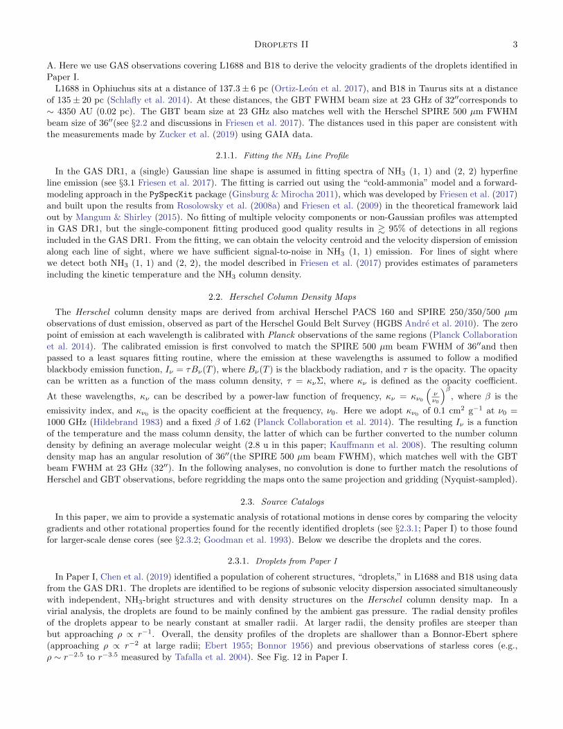
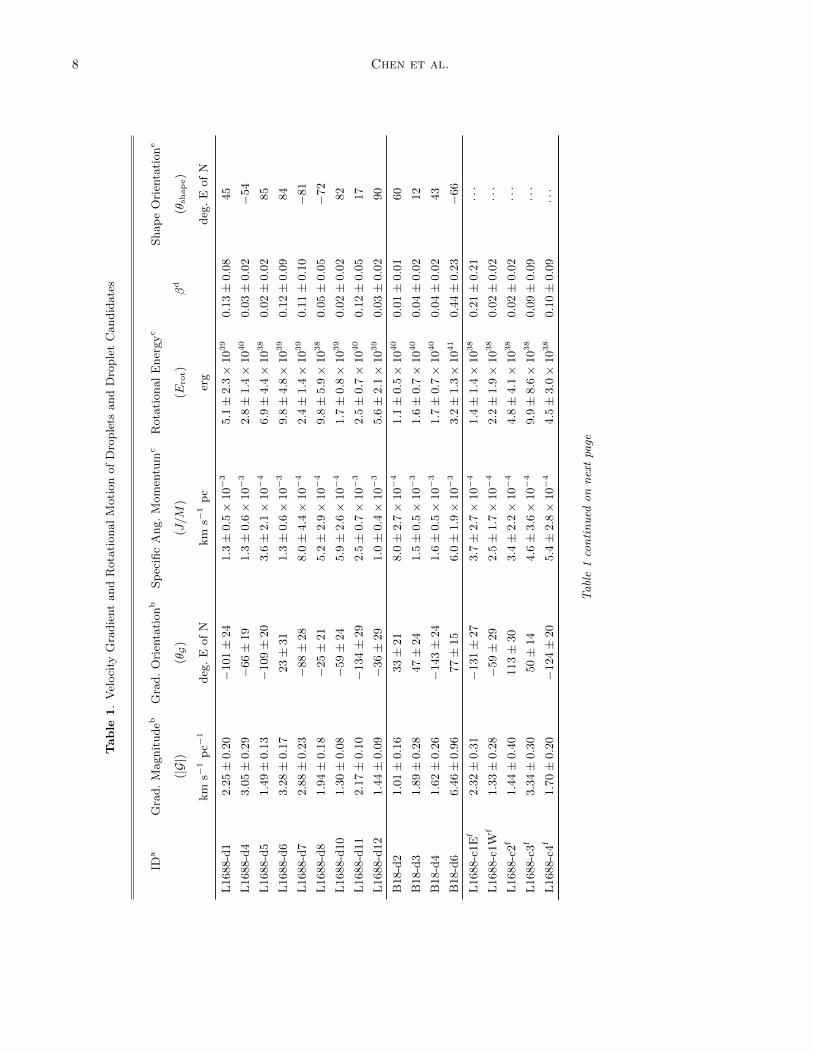
presented in Table 1. Fig. 1, 2, and 3 show the fitted linear velocity fields for the droplets in L1688 and B18 (middle-column panels), in comparison to the observed VLSR (left-column panels). Table 1 lists the resultant velocity gradient

magnitudes and orientations.

1 In this paper, directions in the plane of the sky are expressed in position angles, with the North as the origin and increasing from theNorth to the East.

Page 6

Droplets II 5

–90 0 90

25%

50%

75%

100%

0%

Gradient P.A. [deg]

CDF

Freq

uenc

y0.1 pc0.1 pc

0.1 pc0.1 pc

0.1 pc0.1 pc

0.1 pc0.1 pc

0.1 pc0.1 pc

0.1 pc0.1 pc

22°.8±31°.3(2D) 19°.9±9°.4(Logistic)

–108°.5±20°.1(2D)

–100°.0±20°.2(Logistic)

–65°.6±19°.0(2D)

–61°.0±28°.4(Logistic)

–136°.1±32°.8(2D)

–115°.9±60°.5(Logistic)

–42°.2±28°.2(2D)

–39°.7±18°.2(Logistic)

–101°.3±24°.1(2D)

–83°.2±54°.8(Logistic)

L1688-d1

L1688-d2

L1688-d3

L1688-d4

L1688-d5

L1688-d6

Median VLSR

–0.1

5

+0.1

5

[km s-1]

4.08 km s-1 (Median VLSR)

4.48 km s-1 (Median VLSR)

3.87 km s-1 (Median VLSR)

3.78 km s-1 (Median VLSR)

4.49 km s-1 (Median VLSR)

3.65 km s-1 (Median VLSR)

2.25±0.20km s-1 pc-1 (|Gradient|)

*2.38±0.38km s-1 pc-1 (|Gradient|)

*1.02±0.19km s-1 pc-1 (|Gradient|)

3.05±0.29km s-1 pc-1 (|Gradient|)

1.49±0.13km s-1 pc-1 (|Gradient|)

3.28±0.17km s-1 pc-1 (|Gradient|)

Obsv. 2D Fit

GradientP.A. CDF

|θG–θshape|= 34°.2

|θG–θshape|= 11°.6

|θG–θshape|= 13°.4

|θG–θshape|= 61°.4

*

*

Figure 1. Observed NH3 velocity centroids (VLSR), the 2D linear fit, and the cumulative distribution function (CDF) of pixel-by-pixel velocity gradient position angles, for L1688-d1 to L1688-d6. L1688-d2 and L1688-d3, marked with magenta asterisks,are excluded from subsequent analyses in this paper, due to the small number of available pixels. Left: Observed VLSR of NH3

emission. The contour marks the droplet boundary. The scale bar corresponds to 0.1 pc at the distance of Ophiuchus. The colorscale of each panel has the same stretch, ranging from −0.15 km s−1 to +0.15 km s−1 from the median VLSR of each droplet.Center: Fitted VLSR, based on the 2D linear fit (see §3.1). The color scale is the same as that used for the corresponding panelin the left column. Right: Cumulative distribution function (CDF) of the pixel-by-pixel velocity gradient position angles, basedon the change in VLSR across neighboring pixels. The red vertical line shows the position angle of the gradient from the 2Dlinear fit. The black curve is a logistic function fitted to the CDF, and the vertical black line shows the midpoint of the fittedlogistic function.

Page 7

6 Chen et al.

–90 0 90

25%

50%

75%

100%

0%

Gradient P.A. [deg]

CDF

Freq

uenc

y0.1 pc0.1 pc

0.1 pc0.1 pc

0.1 pc0.1 pc

0.1 pc0.1 pc

0.1 pc0.1 pc

0.1 pc0.1 pc

–36°.1±28°.5(2D)

–11°.5±39°.7(Logistic)

–134°.1±29°.0(2D)

–133°.0±36°.3(Logistic)

–59°.1±23°.5(2D)

–61°.2±30°.9(Logistic)

–154°.5±19°.4(2D)

–31°.2±106°.0(Logistic)

–25°.1±21°.4(2D)

–30°.7±18°.0(Logistic)

–88°.0±27°.9(2D)

–79°.8±30°.3(Logistic)

L1688-d7

L1688-d8

L1688-d9

L1688-d10

L1688-d11

L1688-d12

Median VLSR

–0.1

5

+0.1

5

[km s-1]

3.29 km s-1 (Median VLSR)

3.38 km s-1 (Median VLSR)

4.06 km s-1 (Median VLSR)

4.13 km s-1 (Median VLSR)

3.49 km s-1 (Median VLSR)

3.62 km s-1 (Median VLSR)

2.88±0.23km s-1 pc-1 (|Gradient|)

1.94±0.18km s-1 pc-1 (|Gradient|)

*2.75±0.26km s-1 pc-1 (|Gradient|)

1.30±0.08km s-1 pc-1 (|Gradient|)

2.17±0.10km s-1 pc-1 (|Gradient|)

1.44±0.09km s-1 pc-1 (|Gradient|)

Obsv. 2D Fit

GradientP.A. CDF

|θG–θshape|= 6°.9

|θG–θshape|= 47°.3

|θG–θshape|= 38°.5

|θG–θshape|= 28°.5

|θG–θshape|= 54°.3

*

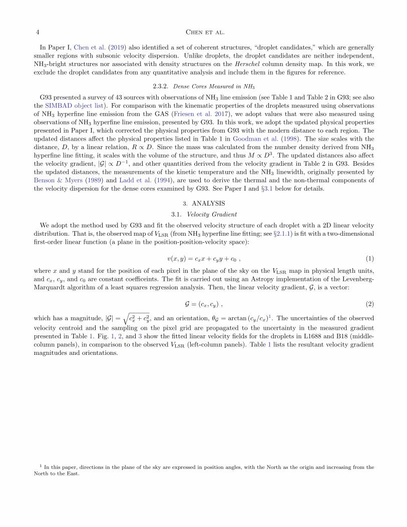
Figure 2. Same as Fig. 1 for L1688-d7 to L1688-d12. L1688-d9, marked with a cyan asterisk, is excluded from subsequentanalyses in this paper, because of the non-linear distribution of VLSR for which a linear velocity fit cannot be generated withouta high uncertainty. Notice that the non-linear distributions of VLSR of L1688-d9 can be identified in their CDFs (in the rightcolumn).

Page 8

Droplets II 7

–90 0 90

25%

50%

75%

100%

0%

Gradient P.A. [deg]

CDF

Freq

uenc

y

0.1 pc0.1 pc

0.1 pc0.1 pc

0.1 pc0.1 pc

0.1 pc0.1 pc

0.1 pc0.1 pc

0.1 pc0.1 pc

77°.1±15°.4(2D) 69°.7±37°.8(Logistic)

–175°.2±21°.0(2D)

4°.7±125°.6(Logistic)

–142°.7±24°.2(2D) 175°.9±75°.7(Logistic)

46°.5±24°.0(2D) 44°.6±31°.0(Logistic)

33°.0±21°.1(2D) 33°.9±38°.8(Logistic)

102°.3±24°.5(2D) 63°.4±100°.6(Logistic)

B18-d1

B18-d2

B18-d3

B18-d4

B18-d5

B18-d6

Median VLSR

–0.1

5

+0.1

5

[km s-1]

5.89 km s-1 (Median VLSR)

6.18 km s-1 (Median VLSR)

5.93 km s-1 (Median VLSR)

6.21 km s-1 (Median VLSR)

6.34 km s-1 (Median VLSR)

6.64 km s-1 (Median VLSR)

*0.37±0.07km s-1 pc-1 (|Gradient|)

1.01±0.16km s-1 pc-1 (|Gradient|)

1.89±0.28km s-1 pc-1 (|Gradient|)

1.62±0.26km s-1 pc-1 (|Gradient|)

*0.91±0.15km s-1 pc-1 (|Gradient|)

6.46±0.96km s-1 pc-1 (|Gradient|)

Obsv. 2D Fit

90 180 270

Gradient P.A. CDF

|θG–θshape|= 27°.2

|θG–θshape|= 35°.0

|θG–θshape|= 6°.0

|θG–θshape|= 36°.9

*

*

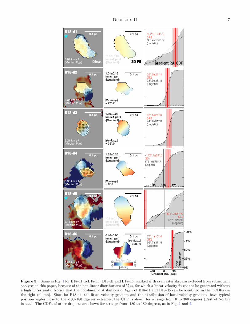
Figure 3. Same as Fig. 1 for B18-d1 to B18-d6. B18-d1 and B18-d5, marked with cyan asterisks, are excluded from subsequentanalyses in this paper, because of the non-linear distributions of VLSR for which a linear velocity fit cannot be generated withouta high uncertainty. Notice that the non-linear distributions of VLSR of B18-d1 and B18-d5 can be identified in their CDFs (inthe right column). Since for B18-d4, the fitted velocity gradient and the distribution of local velocity gradients have typicalposition angles close to the -180/180 degrees extremes, the CDF is shown for a range from 0 to 360 degrees (East of North)instead. The CDFs of other droplets are shown for a range from -180 to 180 degrees, as in Fig. 1 and 2.

Page 9

8 Chen et al.

Table

1.

Vel

oci

tyG

radie

nt

and

Rota

tional

Moti

on

of

Dro

ple

tsand

Dro

ple

tC

andid

ate

s

IDa

Gra

d.

Magnit

udeb

Gra

d.

Ori

enta

tionb

Sp

ecifi

cA

ng.

Mom

entu

mc

Rota

tional

Ener

gyc

Shap

eO

rien

tati

one

(|G|

)(θG

)(J/M

)(E

rot)

βd

(θsh

ape)

km

s−1

pc−

1deg

.E

of

Nkm

s−1

pc

erg

deg

.E

of

N

L1688-d

12.2

5±

0.2

0−

101±

24

1.3±

0.5×

10−3

5.1±

2.3×

1039

0.1

3±

0.0

845

L1688-d

43.0

5±

0.2

9−

66±

19

1.3±

0.6×

10−3

2.8±

1.4×

1040

0.0

3±

0.0

2−

54

L1688-d

51.4

9±

0.1

3−

109±

20

3.6±

2.1×

10−4

6.9±

4.4×

1038

0.0

2±

0.0

285

L1688-d

63.2

8±

0.1

723±

31

1.3±

0.6×

10−3

9.8±

4.8×

1039

0.1

2±

0.0

984

L1688-d

72.8

8±

0.2

3−

88±

28

8.0±

4.4×

10−4

2.4±

1.4×

1039

0.1

1±

0.1

0−

81

L1688-d

81.9

4±

0.1

8−

25±

21

5.2±

2.9×

10−4

9.8±

5.9×

1038

0.0

5±

0.0

5−

72

L1688-d

10

1.3

0±

0.0

8−

59±

24

5.9±

2.6×

10−4

1.7±

0.8×

1039

0.0

2±

0.0

282

L1688-d

11

2.1

7±

0.1

0−

134±

29

2.5±

0.7×

10−3

2.5±

0.7×

1040

0.1

2±

0.0

517

L1688-d

12

1.4

4±

0.0

9−

36±

29

1.0±

0.4×

10−3

5.6±

2.1×

1039

0.0

3±

0.0

290

B18-d

21.0

1±

0.1

633±

21

8.0±

2.7×

10−4

1.1±

0.5×

1040

0.0

1±

0.0

160

B18-d

31.8

9±

0.2

847±

24

1.5±

0.5×

10−3

1.6±

0.7×

1040

0.0

4±

0.0

212

B18-d

41.6

2±

0.2

6−

143±

24

1.6±

0.5×

10−3

1.7±

0.7×

1040

0.0

4±

0.0

243

B18-d

66.4

6±

0.9

677±

15

6.0±

1.9×

10−3

3.2±

1.3×

1041

0.4

4±

0.2

3−

66

L1688-c

1E

f2.3

2±

0.3

1−

131±

27

3.7±

2.7×

10−4

1.4±

1.4×

1038

0.2

1±

0.2

1···

L1688-c

1W

f1.3

3±

0.2

8−

59±

29

2.5±

1.7×

10−4

2.2±

1.9×

1038

0.0

2±

0.0

2···

L1688-c

2f

1.4

4±

0.4

0113±

30

3.4±

2.2×

10−4

4.8±

4.1×

1038

0.0

2±

0.0

2···

L1688-c

3f

3.3

4±

0.3

050±

14

4.6±

3.6×

10−4

9.9±

8.6×

1038

0.0

9±

0.0

9···

L1688-c

4f

1.7

0±

0.2

0−

124±

20

5.4±

2.8×

10−4

4.5±

3.0×

1038

0.1

0±

0.0

9···

Ta

ble

1co

nti

nu

edo

nn

ext

page

Page 10

Droplets II 9Table

1(c

on

tin

ued

)

IDa

Gra

d.

Magnit

udeb

Gra

d.

Ori

enta

tionb

Sp

ecifi

cA

ng.

Mom

entu

mc

Rota

tional

Ener

gyc

Shap

eO

rien

tati

one

(|G|

)(θG

)(J/M

)(E

rot)

βd

(θsh

ape)

km

s−1

pc−

1deg

.E

of

Nkm

s−1

pc

erg

deg

.E

of

N

aL

1688-d

2and

L1688-d

3are

excl

uded

bec

ause

of

the

small

num

ber

of

Nyquis

t-sa

mple

dpix

els

available

toth

elinea

rvel

oci

tyfit.

L1688-d

9,

B18-d

1,

and

B18-d

5are

excl

uded

bec

ause

of

non-l

inea

rvel

oci

tyst

ruct

ure

s,w

hic

hre

sult

inlinea

rfits

wit

hhig

hunce

rtain

ties

.b

Est

imate

dfr

om

2D

linea

rvel

oci

tyfits

and

defi

ned

bet

wee

n−

180

and

180

deg

rees

.See§3

.1.

cE

stim

ate

dbase

don

the

fitt

edvel

oci

tygra

die

nt,

ass

um

ing

that

aro

tati

onalm

oti

on

leads

toth

evel

oci

tygra

die

nt.

The

rota

tional

moti

on

isass

um

edto

be

solid-b

ody,

and

the

rota

ting

body

isass

um

edto

hav

ea

unif

orm

den

sity

.

dT

he

rati

ob

etw

een

the

rota

tional

ener

gy,E

rot,

and

the

abso

lute

valu

eof

gra

vit

ati

onal

pote

nti

al

ener

gy,|Ω

G|.

See§3

.3fo

rdet

ails.

eT

he

posi

tion

angle

of

the

ma

jor

axis

,der

ived

from

NH

3bri

ghtn

ess

ina

pri

nci

pal

com

ponen

tanaly

sis

(PC

A),

and

defi

ned

bet

wee

n−

90

and

90

deg

rees

.See

Pap

erI

for

det

ails.

fL

1688-c

1E

,L

1688-c

1W

,L

1688-c

2,

L1688-c

3,

and

L1688-c

4are

dro

ple

tca

ndid

ate

s(s

ee§2

.3.1

).A

lldro

ple

tca

ndid

ate

ssa

tisf

yth

eva

lidati

on

of

the

gra

die

nt

fits

des

crib

edin§3

.1.

How

ever

,si

nce

they

do

not

sati

sfy

at

least

one

of

the

crit

eria

use

dto

defi

ne

dro

ple

tsin

Pap

erI,

we

do

not

incl

ude

dro

ple

tca

ndid

ate

sin

the

quanti

tati

ve

analy

sis

pre

sente

din

this

pap

er.

They

are

incl

uded

inth

efigure

sfo

rre

fere

nce

.

Page 11

10 Chen et al.

We validate our results from the linear velocity fit with the distributions of the local velocity gradients, measured

from velocity change across neighboring pixels (arrows in the left-column panels of Fig. 1, 2, and 3). In an ideal

case where the observed VLSR map can be fully described by a linear velocity field (Equation 1), the pixel-by-pixel

cumulative distribution function (CDF) for the local velocity gradient orientation would be a step function with the

change (from 0 to 1) occurring at the orientation of the velocity gradient corresponding to the linear velocity field, θG(Equation 2). Thus, the goodness of the linear velocity fit can be estimated by examining the CDFs of local velocity

gradient directions (see the right-column panels of Fig. 1, 2, and 3). In the following analyses, we exclude the droplets

where both the observed VLSR and the CDFs show clear signs of non-linear velocity structures (L1688-d9, B18-d1, and

B18-d5). We also exclude L1688-d2 and L1688-d3 because of the small number of Nyquist-sampled pixels available to

the linear velocity fit.

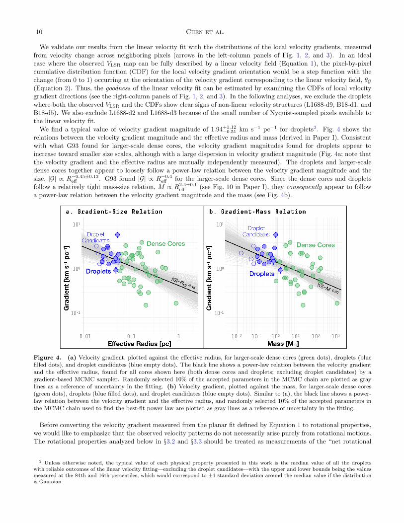
We find a typical value of velocity gradient magnitude of 1.94+1.12−0.51 km s−1 pc−1 for droplets2. Fig. 4 shows the

relations between the velocity gradient magnitude and the effective radius and mass (derived in Paper I). Consistent

with what G93 found for larger-scale dense cores, the velocity gradient magnitudes found for droplets appear to

increase toward smaller size scales, although with a large dispersion in velocity gradient magnitude (Fig. 4a; note that

the velocity gradient and the effective radius are mutually independently measured). The droplets and larger-scale

dense cores together appear to loosely follow a power-law relation between the velocity gradient magnitude and the

size, |G| ∝ R−0.45±0.13eff . G93 found |G| ∝ R−0.4

eff for the larger-scale dense cores. Since the dense cores and droplets

follow a relatively tight mass-size relation, M ∝ R2.4±0.1eff (see Fig. 10 in Paper I), they consequently appear to follow

a power-law relation between the velocity gradient magnitude and the mass (see Fig. 4b).

Figure 4. (a) Velocity gradient, plotted against the effective radius, for larger-scale dense cores (green dots), droplets (bluefilled dots), and droplet candidates (blue empty dots). The black line shows a power-law relation between the velocity gradientand the effective radius, found for all cores shown here (both dense cores and droplets; excluding droplet candidates) by agradient-based MCMC sampler. Randomly selected 10% of the accepted parameters in the MCMC chain are plotted as graylines as a reference of uncertainty in the fitting. (b) Velocity gradient, plotted against the mass, for larger-scale dense cores(green dots), droplets (blue filled dots), and droplet candidates (blue empty dots). Similar to (a), the black line shows a power-law relation between the velocity gradient and the effective radius, and randomly selected 10% of the accepted parameters inthe MCMC chain used to find the best-fit power law are plotted as gray lines as a reference of uncertainty in the fitting.

Before converting the velocity gradient measured from the planar fit defined by Equation 1 to rotational properties,

we would like to emphasize that the observed velocity patterns do not necessarily arise purely from rotational motions.

The rotational properties analyzed below in §3.2 and §3.3 should be treated as measurements of the “net rotational

2 Unless otherwise noted, the typical value of each physical property presented in this work is the median value of all the dropletswith reliable outcomes of the linear velocity fitting—excluding the droplet candidates—with the upper and lower bounds being the valuesmeasured at the 84th and 16th percentiles, which would correspond to ±1 standard deviation around the median value if the distributionis Gaussian.

Page 12

Droplets II 11

motions” that are the results of rotational motions, as well as (but not limited to) turbulence, gravitational infall, and

larger-scale material flow. That is, in an ideal situation where the observed VLSR distribution is a perfect representation

of the 3D motions, these rotational properties would capture any material movement that has a non-zero tangential

component in a cylindrincal coordinate system centered at the core center of mass. In reality, observational effects

may also contribute to the measurements presented in the following analyses, such as the uncertainty in the inclination

angle and the beam effect across the boundary of a core embedded in the molecular cloud (e.g. L1688-d4 shown in

Fig. 1 and L1688-d7 shown in Fig. 2).

3.2. Specific Angular Momentum

Assuming that the observed velocity gradient represents net rotational motion of the droplet, we can derive a specific

angular momentum based on the velocity gradient. Under this assumption, the angular velocity of the rotational motion

is a function of the velocity gradient and inclination:

ω =|G|sin i

, (3)

where i is the inclination angle. Following G93, we adopt sin i = 1 in the following analyses, and thus the angular

velocity has the same magnitude as the velocity gradient, ω = |G|. This represents a lower limit on the angular velocity.

We can then estimate the rotational properties based on the fitted velocity gradient.

If the rotational motion giving rise to the observed velocity gradient is represented by solid-body rotation and the

rotating body has a spherical geometry with a uniform density, the moment of inertia around its rotational axis is

I =2

5MR2 , (4)

where M and R are the mass and radius of the rotating object, respectively. While assuming that all cores are spherical

and have uniform densities can be unrealistic, it has been shown in Paper I that the droplets have small aspect ratios

(. 2; projected on the plane of the sky) and nearly uniform densities within their boundaries. In this work, we adopt

the effective radius of each droplet/dense core for R, derived from the geometric mean of the major and minor axes

based on a principal component analysis of the NH3 brightness distribution (see G93 and Paper I). We would like to

note that most droplets have aspect ratios between 1 and 2, with the exceptions of L1688-d1 and L1688-d6, both of

which have aspect ratios close to 2.5. Since angular momentum J = Iω, the specific angular momentum, defined as

the ratio between the angular momentum and the mass, is

J

M=

2

5ωR2 , (5)

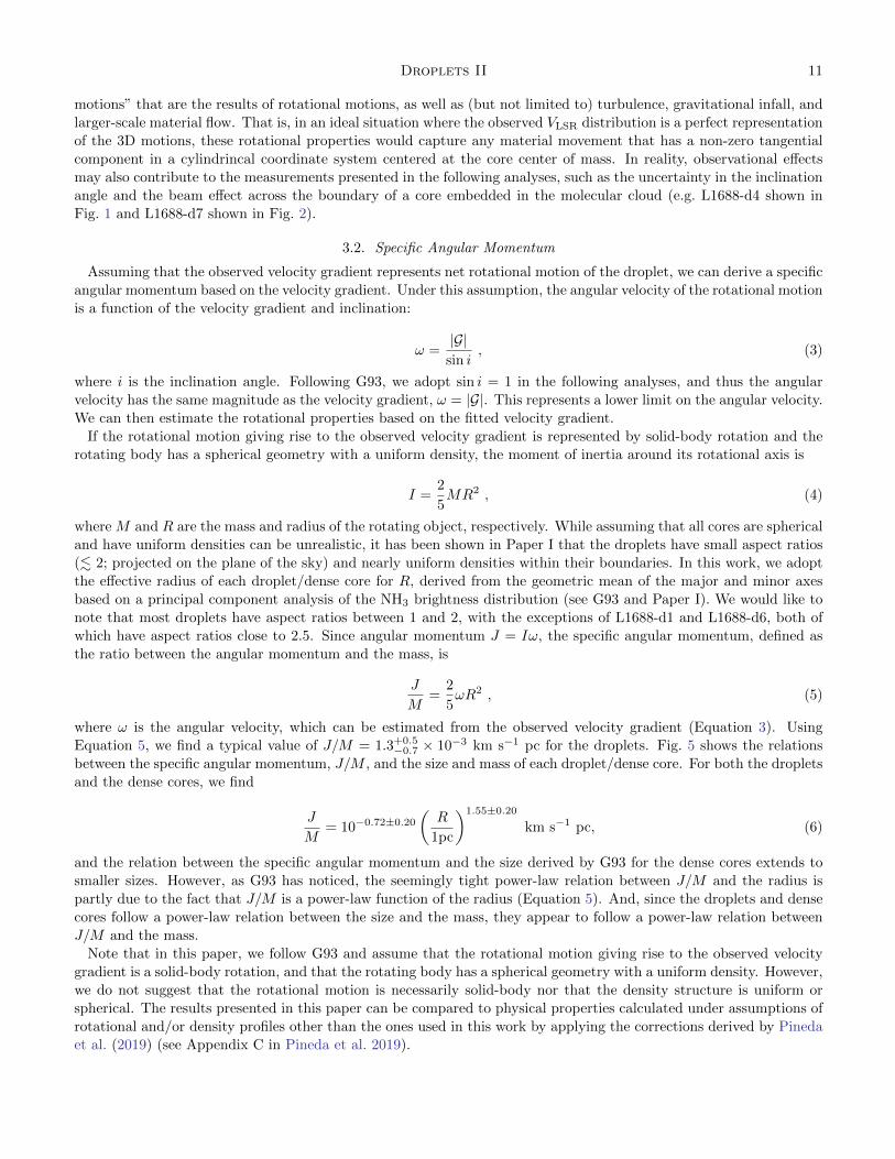
where ω is the angular velocity, which can be estimated from the observed velocity gradient (Equation 3). Using

Equation 5, we find a typical value of J/M = 1.3+0.5−0.7 × 10−3 km s−1 pc for the droplets. Fig. 5 shows the relations

between the specific angular momentum, J/M , and the size and mass of each droplet/dense core. For both the droplets

and the dense cores, we find

J

M= 10−0.72±0.20

(R

1pc

)1.55±0.20

km s−1 pc, (6)

and the relation between the specific angular momentum and the size derived by G93 for the dense cores extends to

smaller sizes. However, as G93 has noticed, the seemingly tight power-law relation between J/M and the radius is

partly due to the fact that J/M is a power-law function of the radius (Equation 5). And, since the droplets and dense

cores follow a power-law relation between the size and the mass, they appear to follow a power-law relation between

J/M and the mass.

Note that in this paper, we follow G93 and assume that the rotational motion giving rise to the observed velocity

gradient is a solid-body rotation, and that the rotating body has a spherical geometry with a uniform density. However,

we do not suggest that the rotational motion is necessarily solid-body nor that the density structure is uniform or

spherical. The results presented in this paper can be compared to physical properties calculated under assumptions of

rotational and/or density profiles other than the ones used in this work by applying the corrections derived by Pineda

et al. (2019) (see Appendix C in Pineda et al. 2019).

Page 13

12 Chen et al.

Figure 5. (a) Specific angular momentum, J/M , plotted against the effective radius, for larger-scale dense cores (greendots), droplets (blue filled dots), and droplet candidates (blue empty dots). The black line shows a power-law relation betweenthe velocity gradient and the effective radius, found for all cores shown here (both dense cores and droplets; excluding dropletcandidates) by a gradient-based MCMC sampler. Randomly selected 10% of the accepted parameters in the MCMC chain areplotted as gray lines as a reference of uncertainty in the fitting. (b) Specific angular momentum, J/M , plotted against themass, for larger-scale dense cores (green dots), droplets (blue filled dots), and droplet candidates (blue empty dots). Similarto (a), the black line shows a power-law relation between the velocity gradient and the effective radius, and randomly selected10% of the accepted parameters in the MCMC chain used to find the best-fit power law are plotted as gray lines as a referenceof uncertainty in the fitting.

3.3. Rotational Energy

For a rotating body with a mass, M , and a radius, R, we can also estimate the rotational energy, Erot, of the

rotational motion giving rise to the observed velocity gradient:

Erot =1

2Iω2 =

1

5MR2ω2 , (7)

assuming solid-body rotation and uniform density. (See Appendix C in Pineda et al. 2019, for detailed derivation of a

general expression for Erot.) We find a typical value of Erot = 1040+0.3−0.8 erg for the droplets.

In a fashion similar to a virial analysis, the rotational energy can be compared to the gravitational potential energy,

ΩG, of the rotating body3:

ΩG = −3

5

GM2

R, (8)

again assuming that the rotating body has a uniform density. In comparison, a sphere of material with a power-law

density distribution, ρ ∝ r−2, has an absolute value of gravitational potential energy, |ΩG|, a factor of ∼ 1.7 larger

than that expressed in Equation 8, and a sphere with a Gaussian density distribution has |ΩG| a factor of ∼ 2 smaller

than that expressed in Equation 8 (Pattle et al. 2015; Kirk et al. 2017). Similar to Paper I, in the following analysis,

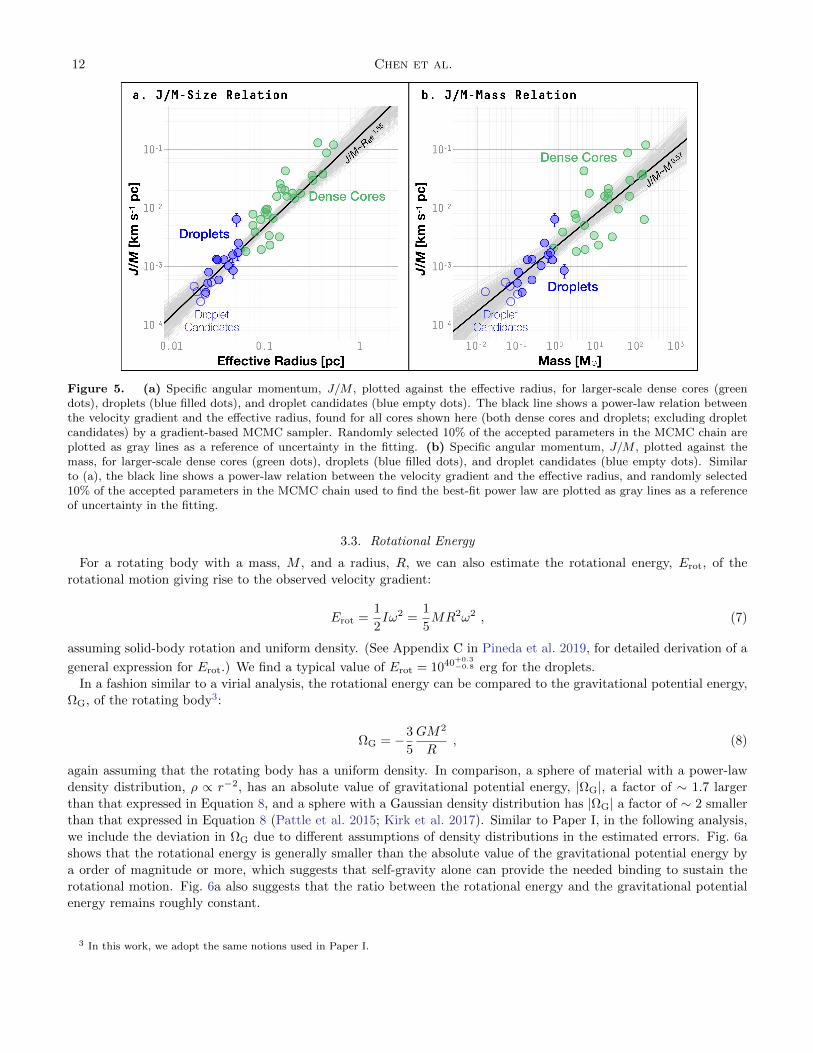
we include the deviation in ΩG due to different assumptions of density distributions in the estimated errors. Fig. 6a

shows that the rotational energy is generally smaller than the absolute value of the gravitational potential energy by

a order of magnitude or more, which suggests that self-gravity alone can provide the needed binding to sustain the

rotational motion. Fig. 6a also suggests that the ratio between the rotational energy and the gravitational potential

energy remains roughly constant.

3 In this work, we adopt the same notions used in Paper I.

Page 14

Droplets II 13

Figure 6. (a) Rotational energy, Erot, plotted against the gravitational potential energy, |ΩG|, for larger-scale dense cores(green dots), droplets (blue filled dots), and droplet candidates (blue empty dots). The red line corresponds to the relation,Erot = |ΩG|, and the red band marks the parameter space within an order of magnitude from this relation. By definition,the ratio between the rotational and gravitational energies, β, is larger toward the top-left of the figure and smaller towardthe bottom-right of the figure. (b) Rotational energy, Erot, plotted against the kinetic energy, ΩK, for larger-scale dense cores(green dots), droplets (blue filled dots), and droplet candidates (blue empty dots). The red line corresponds to the relation,Erot = ΩK, and the red band marks the parameter space within an order of magnitude from this relation.

The ratio between the rotational energy and the gravitational potential energy, β ≡ Erot/ΩG, is sometimes referred

to as the “rotational parameter” (e.g. Dib et al. 2010). The ratio between the rotational and gravitational energies

is often taken as an input parameter to set up the initial conditions for disk and planet formation models (e.g. Allen

et al. 2003; Li et al. 2011; Seifried et al. 2011, 2012), especially to scale the angular velocity of the rotation with respect

to the size and mass of the model. From Equation 7 and 8, we can derive β:

β ≡ Erot

ΩG=

1

3

ω2R3

GM, (9)

with the same assumptions of solid-body rotation and a uniform density, where ω is the angular velocity (see Equation

3). For the droplets, we find a typical value of β = 0.046+0.079−0.024, compared to β ∼ 0.032 found by G93 for larger-scale

dense cores. Including both the droplets and larger-scale dense cores analyzed by G93, we find β ∼ 0.039.

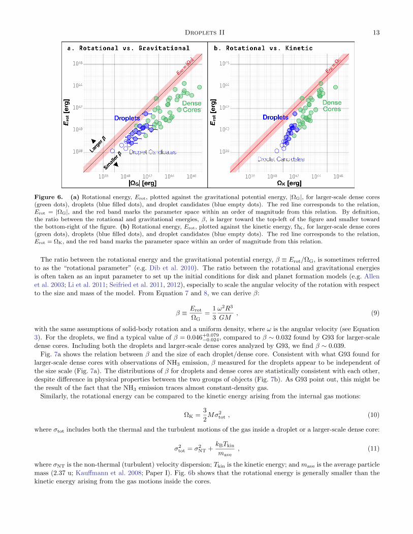
Fig. 7a shows the relation between β and the size of each droplet/dense core. Consistent with what G93 found for

larger-scale dense cores with observations of NH3 emission, β measured for the droplets appear to be independent of

the size scale (Fig. 7a). The distributions of β for droplets and dense cores are statistically consistent with each other,

despite difference in physical properties between the two groups of objects (Fig. 7b). As G93 point out, this might be

the result of the fact that the NH3 emission traces almost constant-density gas.

Similarly, the rotational energy can be compared to the kinetic energy arising from the internal gas motions:

ΩK =3

2Mσ2

tot , (10)

where σtot includes both the thermal and the turbulent motions of the gas inside a droplet or a larger-scale dense core:

σ2tot = σ2

NT +kBTkin

mave, (11)

where σNT is the non-thermal (turbulent) velocity dispersion; Tkin is the kinetic energy; and mave is the average particle

mass (2.37 u; Kauffmann et al. 2008; Paper I). Fig. 6b shows that the rotational energy is generally smaller than the

kinetic energy arising from the gas motions inside the cores.

Page 15

14 Chen et al.

Figure 7. (a) Ratio between rotational and gravitational energies, β, plotted against the effective radius, for larger-scaledense cores (green dots), droplets (blue filled dots), and droplet candidates (blue empty dots). The horizontal black line marksthe median value of β for all cores shown in the figure (both dense cores and droplets; excluding droplet candidates). (b)Distribution of the ratio between rotational and gravitational energies, β, for larger-scale dense cores (green filled histogram)and droplets (excluding droplet candidates; blue histogram). The solid horizontal lines mark the median value of each group.

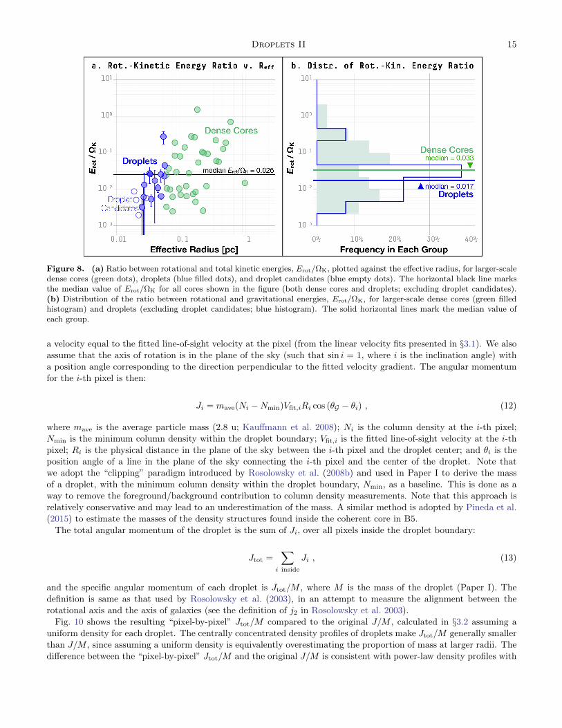
Fig. 8a shows that, similar to β, there is a large scatter in the distribution of Erot/ΩK. Relatively speaking, a

relation between the size and Erot/ΩK is statistically more significant than the one between the size and β, indicated

by a correlation index of 0.87 (versus 0.02 for the size-β distribution) in a Pearson correlation test. However, we note

that a Pearson correlation coefficient of 0.87 cannot be used to determine the existence of a correlation by itself. Fig.

8b shows the overall distributions of Erot/ΩK for the two groups of objects. The median value of Erot/ΩK of the dense

cores is twice as large as the median value of Erot/ΩK of the droplets.

As in the case of the size-β distribution, a large scatter in the size-Erot/ΩK distribution prevents a conclusion. We

note that a potential relation between the size and Erot/ΩK would indicate a deviation from an observed velocity

pattern that is the result of a turbulence scaling law. As Burkert & Bodenheimer (2000) pointed out, ω ∝ σ/R for

such structures (see Equation 14 in Burkert & Bodenheimer 2000), which would make Erot/ΩK ∝ (ωR/σ)2 a constant

with respect to the size. A non-constant relation between the size and Erot/ΩK, if there is one, would suggest that the

observed velocity gradient is not fully the result of internal turbulence within these cores. See Fig. 8.

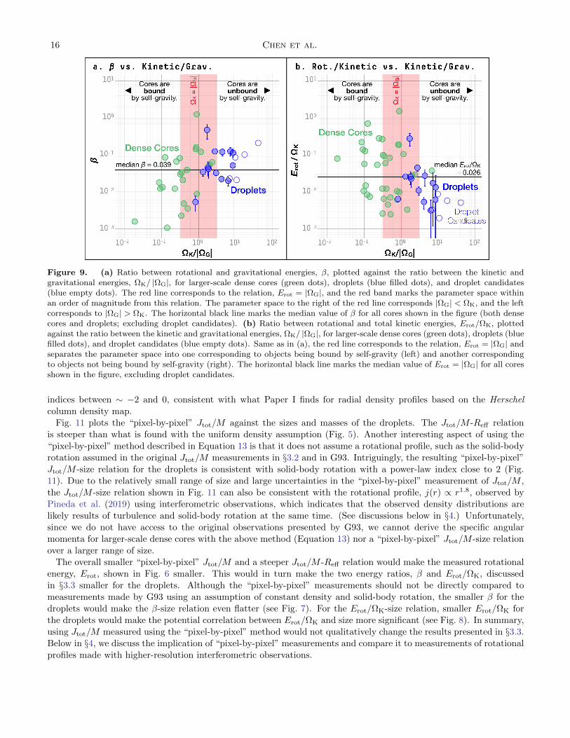
Arguably the most important difference between the dense cores and the droplets is in their gravitational boundedness.

While the droplets and the dense cores follow the same mass-size and linewidth-size relations (see Fig. 9 in Paper I),

the droplets are not bound by self-gravity but are instead bound by the pressure provided by the ambient gas motions

(Paper I). In Fig. 9, we then compare β and Erot/ΩK to the ratio between the internal kinetic energy and the

gravitational potential energy, which characterizes the gravitational boundedness of a core. Fig. 9a suggests that there

is a mild, if any, tendency for less virially bound structures (mostly droplets) to have larger values of β, and again,

the large scatter in β prevents a statistical conclusion of any relation between β and the gravitational boundedness.

On the other hand, Fig 9b suggests that objects that are more bound by self-gravity tend to have larger Erot/ΩK and

those less bound by self-gravity have smaller Erot/ΩK. In §4, we discuss the origin of a potential correlation between

gravitational boundedness and the ratio between rotational, kinetic, and gravitational potential energies.

3.4. Pixel-by-pixel Integration of Angular Momentum

Since Paper I finds that droplets generally have shallow yet not uniform density profiles (see Fig. 12 in Paper I),

we test the idea of using the observed column density map, instead of assuming a uniform density, when calculating

the angular momentum. To derive the total angular momentum of a droplet, we start by calculating the angular

momentum corresponding to each pixel on the observed maps, assuming that at each pixel, the observed mass (column

density observed at the pixel, multiplied by the pixel area in physical units) is rotating around the axis of rotation at

Page 16

Droplets II 15

Figure 8. (a) Ratio between rotational and total kinetic energies, Erot/ΩK, plotted against the effective radius, for larger-scaledense cores (green dots), droplets (blue filled dots), and droplet candidates (blue empty dots). The horizontal black line marksthe median value of Erot/ΩK for all cores shown in the figure (both dense cores and droplets; excluding droplet candidates).(b) Distribution of the ratio between rotational and gravitational energies, Erot/ΩK, for larger-scale dense cores (green filledhistogram) and droplets (excluding droplet candidates; blue histogram). The solid horizontal lines mark the median value ofeach group.

a velocity equal to the fitted line-of-sight velocity at the pixel (from the linear velocity fits presented in §3.1). We also

assume that the axis of rotation is in the plane of the sky (such that sin i = 1, where i is the inclination angle) with

a position angle corresponding to the direction perpendicular to the fitted velocity gradient. The angular momentum

for the i-th pixel is then:

Ji = mave(Ni −Nmin)Vfit,iRi cos (θG − θi) , (12)

where mave is the average particle mass (2.8 u; Kauffmann et al. 2008); Ni is the column density at the i-th pixel;

Nmin is the minimum column density within the droplet boundary; Vfit,i is the fitted line-of-sight velocity at the i-th

pixel; Ri is the physical distance in the plane of the sky between the i-th pixel and the droplet center; and θi is the

position angle of a line in the plane of the sky connecting the i-th pixel and the center of the droplet. Note that

we adopt the “clipping” paradigm introduced by Rosolowsky et al. (2008b) and used in Paper I to derive the mass

of a droplet, with the minimum column density within the droplet boundary, Nmin, as a baseline. This is done as a

way to remove the foreground/background contribution to column density measurements. Note that this approach is

relatively conservative and may lead to an underestimation of the mass. A similar method is adopted by Pineda et al.

(2015) to estimate the masses of the density structures found inside the coherent core in B5.

The total angular momentum of the droplet is the sum of Ji, over all pixels inside the droplet boundary:

Jtot =∑

i inside

Ji , (13)

and the specific angular momentum of each droplet is Jtot/M , where M is the mass of the droplet (Paper I). The

definition is same as that used by Rosolowsky et al. (2003), in an attempt to measure the alignment between the

rotational axis and the axis of galaxies (see the definition of j2 in Rosolowsky et al. 2003).

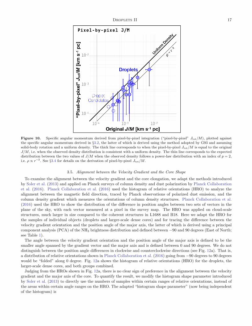
Fig. 10 shows the resulting “pixel-by-pixel” Jtot/M compared to the original J/M , calculated in §3.2 assuming a

uniform density for each droplet. The centrally concentrated density profiles of droplets make Jtot/M generally smaller

than J/M , since assuming a uniform density is equivalently overestimating the proportion of mass at larger radii. The

difference between the “pixel-by-pixel” Jtot/M and the original J/M is consistent with power-law density profiles with

Page 17

16 Chen et al.

Figure 9. (a) Ratio between rotational and gravitational energies, β, plotted against the ratio between the kinetic andgravitational energies, ΩK/ |ΩG|, for larger-scale dense cores (green dots), droplets (blue filled dots), and droplet candidates(blue empty dots). The red line corresponds to the relation, Erot = |ΩG|, and the red band marks the parameter space withinan order of magnitude from this relation. The parameter space to the right of the red line corresponds |ΩG| < ΩK, and the leftcorresponds to |ΩG| > ΩK. The horizontal black line marks the median value of β for all cores shown in the figure (both densecores and droplets; excluding droplet candidates). (b) Ratio between rotational and total kinetic energies, Erot/ΩK, plottedagainst the ratio between the kinetic and gravitational energies, ΩK/ |ΩG|, for larger-scale dense cores (green dots), droplets (bluefilled dots), and droplet candidates (blue empty dots). Same as in (a), the red line corresponds to the relation, Erot = |ΩG| andseparates the parameter space into one corresponding to objects being bound by self-gravity (left) and another correspondingto objects not being bound by self-gravity (right). The horizontal black line marks the median value of Erot = |ΩG| for all coresshown in the figure, excluding droplet candidates.

indices between ∼ −2 and 0, consistent with what Paper I finds for radial density profiles based on the Herschel

column density map.

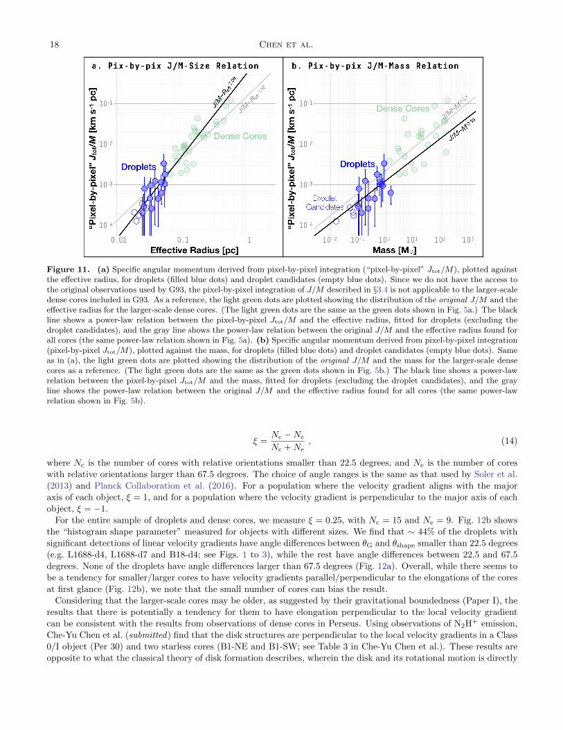
Fig. 11 plots the “pixel-by-pixel” Jtot/M against the sizes and masses of the droplets. The Jtot/M -Reff relation

is steeper than what is found with the uniform density assumption (Fig. 5). Another interesting aspect of using the

“pixel-by-pixel” method described in Equation 13 is that it does not assume a rotational profile, such as the solid-body

rotation assumed in the original Jtot/M measurements in §3.2 and in G93. Intriguingly, the resulting “pixel-by-pixel”

Jtot/M -size relation for the droplets is consistent with solid-body rotation with a power-law index close to 2 (Fig.

11). Due to the relatively small range of size and large uncertainties in the “pixel-by-pixel” measurement of Jtot/M ,

the Jtot/M -size relation shown in Fig. 11 can also be consistent with the rotational profile, j(r) ∝ r1.8, observed by

Pineda et al. (2019) using interferometric observations, which indicates that the observed density distributions are

likely results of turbulence and solid-body rotation at the same time. (See discussions below in §4.) Unfortunately,

since we do not have access to the original observations presented by G93, we cannot derive the specific angular

momenta for larger-scale dense cores with the above method (Equation 13) nor a “pixel-by-pixel” Jtot/M -size relation

over a larger range of size.

The overall smaller “pixel-by-pixel” Jtot/M and a steeper Jtot/M -Reff relation would make the measured rotational

energy, Erot, shown in Fig. 6 smaller. This would in turn make the two energy ratios, β and Erot/ΩK, discussed

in §3.3 smaller for the droplets. Although the “pixel-by-pixel” measurements should not be directly compared to

measurements made by G93 using an assumption of constant density and solid-body rotation, the smaller β for the

droplets would make the β-size relation even flatter (see Fig. 7). For the Erot/ΩK-size relation, smaller Erot/ΩK for

the droplets would make the potential correlation between Erot/ΩK and size more significant (see Fig. 8). In summary,

using Jtot/M measured using the “pixel-by-pixel” method would not qualitatively change the results presented in §3.3.

Below in §4, we discuss the implication of “pixel-by-pixel” measurements and compare it to measurements of rotational

profiles made with higher-resolution interferometric observations.

Page 18

Droplets II 17

Figure 10. Specific angular momentum derived from pixel-by-pixel integration (“pixel-by-pixel” Jtot/M), plotted againstthe specific angular momentum derived in §3.2, the latter of which is derived using the method adopted by G93 and assumingsolid-body rotation and a uniform density. The thick line corresponds to when the pixel-by-pixel Jtot/M is equal to the originalJ/M , i.e. when the observed density distribution is consistent with a uniform density. The thin line corresponds to the expecteddistribution between the two values of J/M when the observed density follows a power-law distribution with an index of p = 2,i.e. ρ ∝ r−2. See §3.4 for details on the derivation of pixel-by-pixel Jtot/M .

3.5. Alignment between the Velocity Gradient and the Core Shape

To examine the alignment between the velocity gradient and the core elongation, we adapt the methods introduced

by Soler et al. (2013) and applied on Planck surveys of column density and dust polarization by Planck Collaboration

et al. (2016). Planck Collaboration et al. (2016) used the histogram of relative orientations (HRO) to analyze the

alignment between the magnetic field direction, traced by Planck observations of polarized dust emission, and the

column density gradient which measures the orientations of column density structures. Planck Collaboration et al.

(2016) used the HRO to show the distribution of the difference in position angles between two sets of vectors in the

plane of the sky, with each vector measured at a pixel in the survey map. The HRO was applied on cloud-scale

structures, much larger in size compared to the coherent structures in L1688 and B18. Here we adapt the HRO for

the samples of individual objects (droplets and larger-scale dense cores) and for tracing the difference between the

velocity gradient orientation and the position angle of the major axis, the latter of which is derived using a principal

component analysis (PCA) of the NH3 brightness distribution and defined between −90 and 90 degrees (East of North;

see Table 1).

The angle between the velocity gradient orientation and the position angle of the major axis is defined to be the

smaller angle spanned by the gradient vector and the major axis and is defined between 0 and 90 degrees. We do not

distinguish between the position angle differences in clockwise and counterclockwise directions (see Fig. 12a). That is,

a distribution of relative orientations shown in Planck Collaboration et al. (2016) going from −90 degrees to 90 degrees

would be “folded” along 0 degree. Fig. 12a shows the histogram of relative orientations (HRO) for the droplets, the

larger-scale dense cores, and both groups combined.

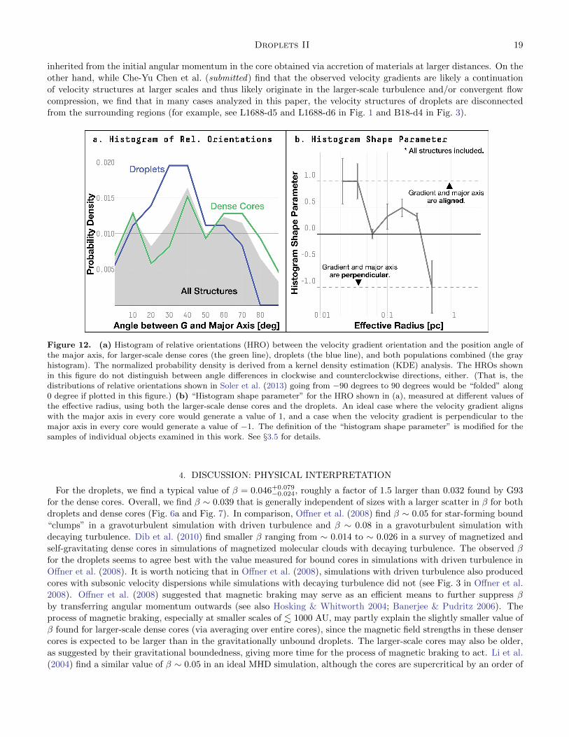
Judging from the HROs shown in Fig. 12a, there is no clear sign of preference in the alignment between the velocity

gradient and the major axis of the core. To quantify the result, we modify the histogram shape parameter introduced

by Soler et al. (2013) to directly use the numbers of samples within certain ranges of relative orientations, instead of

the areas within certain angle ranges on the HRO. The adapted “histogram shape parameter” (now being independent

of the histogram) is

Page 19

18 Chen et al.

Figure 11. (a) Specific angular momentum derived from pixel-by-pixel integration (“pixel-by-pixel” Jtot/M), plotted againstthe effective radius, for droplets (filled blue dots) and droplet candidates (empty blue dots). Since we do not have the access tothe original observations used by G93, the pixel-by-pixel integration of J/M described in §3.4 is not applicable to the larger-scaledense cores included in G93. As a reference, the light green dots are plotted showing the distribution of the original J/M and theeffective radius for the larger-scale dense cores. (The light green dots are the same as the green dots shown in Fig. 5a.) The blackline shows a power-law relation between the pixel-by-pixel Jtot/M and the effective radius, fitted for droplets (excluding thedroplet candidates), and the gray line shows the power-law relation between the original J/M and the effective radius found forall cores (the same power-law relation shown in Fig. 5a). (b) Specific angular momentum derived from pixel-by-pixel integration(pixel-by-pixel Jtot/M), plotted against the mass, for droplets (filled blue dots) and droplet candidates (empty blue dots). Sameas in (a), the light green dots are plotted showing the distribution of the original J/M and the mass for the larger-scale densecores as a reference. (The light green dots are the same as the green dots shown in Fig. 5b.) The black line shows a power-lawrelation between the pixel-by-pixel Jtot/M and the mass, fitted for droplets (excluding the droplet candidates), and the grayline shows the power-law relation between the original J/M and the effective radius found for all cores (the same power-lawrelation shown in Fig. 5b).

ξ =Nc −Ne

Nc +Ne, (14)

where Nc is the number of cores with relative orientations smaller than 22.5 degrees, and Ne is the number of cores

with relative orientations larger than 67.5 degrees. The choice of angle ranges is the same as that used by Soler et al.

(2013) and Planck Collaboration et al. (2016). For a population where the velocity gradient aligns with the major

axis of each object, ξ = 1, and for a population where the velocity gradient is perpendicular to the major axis of each

object, ξ = −1.

For the entire sample of droplets and dense cores, we measure ξ = 0.25, with Nc = 15 and Ne = 9. Fig. 12b shows

the “histogram shape parameter” measured for objects with different sizes. We find that ∼ 44% of the droplets with

significant detections of linear velocity gradients have angle differences between θG and θshape smaller than 22.5 degrees

(e.g. L1688-d4, L1688-d7 and B18-d4; see Figs. 1 to 3), while the rest have angle differences between 22.5 and 67.5

degrees. None of the droplets have angle differences larger than 67.5 degrees (Fig. 12a). Overall, while there seems to

be a tendency for smaller/larger cores to have velocity gradients parallel/perpendicular to the elongations of the cores

at first glance (Fig. 12b), we note that the small number of cores can bias the result.

Considering that the larger-scale cores may be older, as suggested by their gravitational boundedness (Paper I), the

results that there is potentially a tendency for them to have elongation perpendicular to the local velocity gradient

can be consistent with the results from observations of dense cores in Perseus. Using observations of N2H+ emission,

Che-Yu Chen et al. (submitted) find that the disk structures are perpendicular to the local velocity gradients in a Class

0/I object (Per 30) and two starless cores (B1-NE and B1-SW; see Table 3 in Che-Yu Chen et al.). These results are

opposite to what the classical theory of disk formation describes, wherein the disk and its rotational motion is directly

Page 20

Droplets II 19

inherited from the initial angular momentum in the core obtained via accretion of materials at larger distances. On the

other hand, while Che-Yu Chen et al. (submitted) find that the observed velocity gradients are likely a continuation

of velocity structures at larger scales and thus likely originate in the larger-scale turbulence and/or convergent flow

compression, we find that in many cases analyzed in this paper, the velocity structures of droplets are disconnected

from the surrounding regions (for example, see L1688-d5 and L1688-d6 in Fig. 1 and B18-d4 in Fig. 3).

Figure 12. (a) Histogram of relative orientations (HRO) between the velocity gradient orientation and the position angle ofthe major axis, for larger-scale dense cores (the green line), droplets (the blue line), and both populations combined (the grayhistogram). The normalized probability density is derived from a kernel density estimation (KDE) analysis. The HROs shownin this figure do not distinguish between angle differences in clockwise and counterclockwise directions, either. (That is, thedistributions of relative orientations shown in Soler et al. (2013) going from −90 degrees to 90 degrees would be “folded” along0 degree if plotted in this figure.) (b) “Histogram shape parameter” for the HRO shown in (a), measured at different values ofthe effective radius, using both the larger-scale dense cores and the droplets. An ideal case where the velocity gradient alignswith the major axis in every core would generate a value of 1, and a case when the velocity gradient is perpendicular to themajor axis in every core would generate a value of −1. The definition of the “histogram shape parameter” is modified for thesamples of individual objects examined in this work. See §3.5 for details.

4. DISCUSSION: PHYSICAL INTERPRETATION

For the droplets, we find a typical value of β = 0.046+0.079−0.024, roughly a factor of 1.5 larger than 0.032 found by G93

for the dense cores. Overall, we find β ∼ 0.039 that is generally independent of sizes with a larger scatter in β for both

droplets and dense cores (Fig. 6a and Fig. 7). In comparison, Offner et al. (2008) find β ∼ 0.05 for star-forming bound

“clumps” in a gravoturbulent simulation with driven turbulence and β ∼ 0.08 in a gravoturbulent simulation with

decaying turbulence. Dib et al. (2010) find smaller β ranging from ∼ 0.014 to ∼ 0.026 in a survey of magnetized and

self-gravitating dense cores in simulations of magnetized molecular clouds with decaying turbulence. The observed β

for the droplets seems to agree best with the value measured for bound cores in simulations with driven turbulence in

Offner et al. (2008). It is worth noticing that in Offner et al. (2008), simulations with driven turbulence also produced

cores with subsonic velocity dispersions while simulations with decaying turbulence did not (see Fig. 3 in Offner et al.

2008). Offner et al. (2008) suggested that magnetic braking may serve as an efficient means to further suppress β

by transferring angular momentum outwards (see also Hosking & Whitworth 2004; Banerjee & Pudritz 2006). The

process of magnetic braking, especially at smaller scales of . 1000 AU, may partly explain the slightly smaller value of

β found for larger-scale dense cores (via averaging over entire cores), since the magnetic field strengths in these denser

cores is expected to be larger than in the gravitationally unbound droplets. The larger-scale cores may also be older,

as suggested by their gravitational boundedness, giving more time for the process of magnetic braking to act. Li et al.

(2004) find a similar value of β ∼ 0.05 in an ideal MHD simulation, although the cores are supercritical by an order of

Page 21

20 Chen et al.

magnitude. A study of both gravitationally bound and pressure bound coherent structures in simulations is needed to

further examine the physical processes involved in the evolution of rotational motions in droplets and coherent cores.

Considering that the larger-scale dense cores may be older as suggested by Paper I, the relation between the ro-

tational, kinetic, and gravitational potential energies, shown in Fig. 9, may be consistent with a picture where the

gravitational infall provides the initial angular momentum and the rotational motions co-evolve with gravity. A non-

constant size-Erot/ΩK relation, if there is one (see Fig. 8), would also indicate that the measured velocity gradient

is not fully the result of turbulence within cores. On the other hand, Burkert & Bodenheimer (2000) find that the

observed velocity pattern can be the result of a turbulence scaling law. For turbulence dominated gas with a Larson’s

law-like power-law relation between velocity dispersion and the size, δv ∼ r0.5, there exists a relation between the

observed specific angular momentum and the size, J/M ∝ R1.5, in the model presented by Burkert & Bodenheimer

(2000). Chen & Ostriker (2018) also find J/M ∝ R1.5 in a survey of gravitationally bound dense cores in MHD sim-

ulations and conclude that the rotational motion is acquired from ambient turbulence. Similarly, Che-Yu Chen et al.

(submitted) conclude that the observed velocity structures likely originate in the large-scale turbulence or convergent

flow, using observations of N2H+ of dense cores in Perseus.

Using Very Large Array (VLA) interferometric observations of NH3 (1, 1) emission, Pineda et al. (2019) examine

the interior velocity structures in two Class 0 objects and one first hydrostatic core candidate. Resolving the internal

velocity structures within these cores, Pineda et al. (2019) are able to derive the radial profile of specific angular

momentum, j(r), and find j(r) ∝ r1.8. The result suggests that the observed “net rotational motion” in cores is not

purely solid-body rotation as usually assumed, which would result in j(r) ∝ r2, and the turbulence is involved in

creating the observed velocity structures in cores. In this study, we derive a J/M -size relation consistent with that

derived by G93, J/M ∝ R1.5, assuming that the observed cores have constant densities and the velocity structure

is due to solid-body rotation (see §3.2). Using column density maps derived from Herschel observations, we also

derive a “pixel-by-pixel” Jtot/M -size relation, Jtot/M ∝ R2.08 for the droplets over a limited range of sizes (see §3.4),

without having to assume either a constant density or solid-body rotation. Again, as G93 pointed out, measurements

of rotational quantities based on observations represent a “net rotational motion” instead of indicating that the core

is actually rotating in a solid-body manner. The measurement is also likely affected by observational effects such as

the uncertainty in the viewing angle. More studies need to be done on the co-evolution between gravity, turbulence,

the magnetic field, and the rotational motion. In particular, it could benefit from analyses of velocity gradients in the

interiors of dense cores found in higher-resolution observations of higher-density tracers, such as those observed by the

MASSES survey (Stephens et al. 2018).

5. CONCLUSION

In this paper, we use the data from Green Bank Ammonia Survey (GAS; Friesen et al. 2017) and examine the

internal velocity structures of the droplets—sub-0.1 coherent core-like structures, in two nearby star forming regions,

L1688 in Ophiuchus and B18 in Taurus (Paper I). A linear velocity field is fitted to the observed VLSR, derived from

NH3 hyperfine line fitting (Fig. 1, 2, and 3). The resulting velocity gradients of the droplets are found to follow a

power-law relation between the gradient magnitude and the size similar to the relation found for larger-scale dense

cores by G93, although with some dispersion in the fitted velocity gradient (Fig. 4).

Following G93, we assume that the fitted velocity gradient arises from solid-body rotation of a rotating sphere with a

uniform density. We derive the specific angular momentum, J/M , and find that both the droplets and the larger-scale

dense cores appear to follow a relatively tight relation between J/M and the effective radius (Fig. 5a). The relation

between J/M and the size found for droplets is consistent with what G93 find for larger-scale dense cores, J/M ∝ R1.5.

However, we note that the tight correlation is at least partly due to the potentially wrong assumptions of solid-body

rotation and a uniform density for the observed core. Also, as numerous works on simulations and observations have

pointed out, a J/M -size relation of J/M ∝ R1.5 is consistent with turbulent motions that follow a Larson’s law-like

scaling relation (e.g. Burkert & Bodenheimer 2000; Chen & Ostriker 2018).

We examine the rotational energy of the assumed solid-body rotation that gives rise to the fitted velocity gradient. We

find that the rotational energy, Erot, is generally smaller than the gravitational energy, ΩG by an order of magnitude

or more (Fig. 6a), which suggests that self-gravity alone can provide the needed binding to sustain the rotational

motion. We also compare Erot to the internal kinetic energy calculated for the thermal and non-thermal motions of

gas inside the droplet/larger-scale dense core, ΩK (Fig. 6b). We find Erot is generally smaller than ΩK, suggesting

Page 22

Droplets II 21

that the rotational contribution to the observed linewidth is smaller than the contribution from thermal and turbulent

motions inside droplets and larger-scale dense cores.

For the droplets, we find a typical value of the ratio between the rotational energy and the gravitational potential

energy, β, of 0.046+0.079−0.024. Overall, for the entire population including both the droplets and the larger-scale dense cores

examined in G93, we find β ∼ 0.039. Consistent with what G93 found for larger-scale dense cores, we find that β

generally independent of the size scale for the droplets. The result extends the scale independency of β down to a size

scale of ∼ 0.02 pc. As G93 pointed out, this can be due to the fact that NH3 emission traces almost constant-density

gas. Similarly, there is a large scatter in the distribution of Erot/ΩK .

We also derive the specific angular momentum directly from the Herschel column density maps, instead of having

to assume a uniform density and solid-body rotation for each droplet. Consistent with what Paper I finds for the

radial density profiles, the difference between the “pixel-by-pixel” specific angular momentum and the original value

is consistent with power-law density profiles with indices between −2 and 0 (Fig. 10). Consequently, with the “pixel-

by-pixel” specific angular momentum, we find a steeper relation between the specific angular momentum and the size

(Fig. 11).

Adapting the methods used by Soler et al. (2013) and Planck Collaboration et al. (2016) to quantify the alignment

between the polarization and the orientation of column density structures, we show that there is barely any indication

of preferred alignment between the velocity gradient and the major axis of a core included in this work (Fig. 12a). The

adapted “histogram shape parameter” seems to suggest that there could be a tendency for smaller cores to have velocity

gradients parallel to the major axes. However, the small number of samples prevents any statistical conclusions.

As shown in this study, the observations of velocity gradients in droplets not only provide an observational constraint

on the measurement of “net rotational motions” at size scales . 0.1 pc, they may also provide a look into the velocity

structures at a potentially earlier stage in core evolution. The results presented in this paper suggest a tight relation

between gravity, turbulence, and the rotational motion. More research needs to be done to study the co-evolution of

rotation with other physical processes in the process of core formation.

This work was supported by a Cottrell Scholar Award. The National Radio Astronomy Observatory is a facility of

the National Science Foundation operated under cooperative agreement by Associated Universities, Inc.

Facilities: GBT (KFPA+VEGAS), Herschel Space Observatory (PACS+SPIRE)

Software: astropy(TheAstropyCollaborationetal.2018),Glue(Beaumontetal.2015;Robitailleetal.2017),PySpecKit

(Ginsburg & Mirocha 2011), RADMC-3D (Dullemond et al. 2012)

REFERENCES

Allen, A., Li, Z.-Y., & Shu, F. H. 2003, ApJ, 599, 363,

doi: 10.1086/379243

Andre, P., Di Francesco, J., Ward-Thompson, D., et al.

2014, Protostars and Planets VI, 27,

doi: 10.2458/azu uapress 9780816531240-ch002

Andre, P., Men’shchikov, A., Bontemps, S., et al. 2010,

A&A, 518, L102

Arquilla, R. 1984, PhD thesis, UNIVERSITY OF

MASSACHUSETTS.

Arquilla, R., & Goldsmith, P. F. 1985, ApJ, 297, 436,

doi: 10.1086/163542

—. 1986, ApJ, 303, 356, doi: 10.1086/164082

Arzoumanian, D., Andre, P., Peretto, N., & Konyves, V.

2013, A&A, 553, A119,

doi: 10.1051/0004-6361/201220822

Banerjee, R., & Pudritz, R. E. 2006, ApJ, 641, 949,

doi: 10.1086/500496

Beaumont, C., Goodman, A., & Greenfield, P. 2015, in

Astronomical Society of the Pacific Conference Series,

Vol. 495, Astronomical Data Analysis Software an

Systems XXIV (ADASS XXIV), ed. A. R. Taylor &

E. Rosolowsky, 101

Benson, P. J., & Myers, P. C. 1989, ApJS, 71, 89,

doi: 10.1086/191365

Bonnor, W. B. 1956, MNRAS, 116, 351,

doi: 10.1093/mnras/116.3.351

Burkert, A., & Bodenheimer, P. 2000, ApJ, 543, 822,

doi: 10.1086/317122

Chen, C.-Y., & Ostriker, E. C. 2018, ApJ, 865, 34,

doi: 10.3847/1538-4357/aad905

Page 23

22 Chen et al.

Chen, H. H.-H., Pineda, J. E., Goodman, A. A., et al. 2019,

ApJ, 877, 93, doi: 10.3847/1538-4357/ab1a40

Dib, S., Hennebelle, P., Pineda, J. E., et al. 2010, ApJ, 723,

425, doi: 10.1088/0004-637X/723/1/425

Dullemond, C. P., Juhasz, A., Pohl, A., et al. 2012,

RADMC-3D: A multi-purpose radiative transfer tool,

Astrophysics Source Code Library.

http://ascl.net/1202.015

Ebert, R. 1955, ZA, 37, 217

Friesen, R. K., Di Francesco, J., Shirley, Y. L., & Myers,

P. C. 2009, ApJ, 697, 1457,

doi: 10.1088/0004-637X/697/2/1457

Friesen, R. K., Pineda, J. E., co-PIs, et al. 2017, ApJ, 843,

63, doi: 10.3847/1538-4357/aa6d58

Ginsburg, A., & Mirocha, J. 2011, PySpecKit: Python

Spectroscopic Toolkit, Astrophysics Source Code Library.

http://ascl.net/1109.001

Goldsmith, P. F., & Arquilla, R. 1985, in IN: Protostars

and planets II (A86-12626 03-90). Tucson, AZ, University

of Arizona Press, 1985, p. 137-149. Research supported

by the Observatoire de Paris and NSF., 137–149

Goodman, A. A., Barranco, J. A., Wilner, D. J., & Heyer,

M. H. 1998, ApJ, 504, 223, doi: 10.1086/306045

Goodman, A. A., Benson, P. J., Fuller, G. A., & Myers,

P. C. 1993, ApJ, 406, 528, doi: 10.1086/172465

Hacar, A., Tafalla, M., Kauffmann, J., & Kovacs, A. 2013,

A&A, 554, A55, doi: 10.1051/0004-6361/201220090

Hildebrand, R. H. 1983, QJRAS, 24, 267

Hosking, J. G., & Whitworth, A. P. 2004, MNRAS, 347,

994, doi: 10.1111/j.1365-2966.2004.07273.x

Kauffmann, J., Bertoldi, F., Bourke, T. L., Evans, II, N. J.,

& Lee, C. W. 2008, A&A, 487, 993,

doi: 10.1051/0004-6361:200809481

Kirk, H., Friesen, R. K., Pineda, J. E., et al. 2017, ApJ,

846, 144, doi: 10.3847/1538-4357/aa8631

Ladd, E. F., Myers, P. C., & Goodman, A. A. 1994, ApJ,

433, 117, doi: 10.1086/174629

Li, P. S., Norman, M. L., Mac Low, M.-M., & Heitsch, F.

2004, ApJ, 605, 800, doi: 10.1086/382652

Li, Z.-Y., Krasnopolsky, R., & Shang, H. 2011, ApJ, 738,

doi: 10.1088/0004-637X/738/2/180

Mangum, J. G., & Shirley, Y. L. 2015, PASP, 127, 266,

doi: 10.1086/680323

McKee, C. F., & Ostriker, E. C. 2007, ARA&A, 45, 565,

doi: 10.1146/annurev.astro.45.051806.110602

Monsch, K., Pineda, J. E., Liu, H. B., et al. 2018, ApJ, 861,

77, doi: 10.3847/1538-4357/aac8da

Myers, P. C. 2009, ApJ, 700, 1609,

doi: 10.1088/0004-637X/700/2/1609

Offner, S. S. R., Klein, R. I., & McKee, C. F. 2008, ApJ,

686, 1174, doi: 10.1086/590238

Ortiz-Leon, G. N., Loinard, L., Kounkel, M. A., et al. 2017,

ApJ, 834, 141, doi: 10.3847/1538-4357/834/2/141

Padoan, P., Federrath, C., Chabrier, G., et al. 2014,

Protostars and Planets VI, 77,

doi: 10.2458/azu uapress 9780816531240-ch004

Pattle, K., Ward-Thompson, D., Kirk, J. M., et al. 2015,

MNRAS, 450, 1094, doi: 10.1093/mnras/stv376

Pineda, J. E., Goodman, A. A., Arce, H. G., et al. 2010,

ApJL, 712, L116, doi: 10.1088/2041-8205/712/1/L116

Pineda, J. E., Zhao, B., Schmiedeke, A., et al. 2019, arXiv

e-prints, arXiv:1906.05578.

https://arxiv.org/abs/1906.05578

Pineda, J. E., Offner, S. S. R., Parker, R. J., et al. 2015,

Nature, 518, 213, doi: 10.1038/nature14166

Planck Collaboration, Abergel, A., Ade, P. A. R., et al.

2014, A&A, 571, A11, doi: 10.1051/0004-6361/201323195

Planck Collaboration, Ade, P. A. R., Aghanim, N., et al.

2016, A&A, 586, doi: 10.1051/0004-6361/201525896

Robitaille, T., Beaumont, C., Qian, P., Borkin, M., &

Goodman, A. 2017, glueviz v0.13.1: multidimensional

data exploration glueviz v0.13.1: multidimensional data

exploration, doi: 10.5281/zenodo.1237692.

https://doi.org/10.5281/zenodo.1237692

Rosolowsky, E., Engargiola, G., Plambeck, R., & Blitz, L.

2003, ApJ, 599, 258, doi: 10.1086/379166

Rosolowsky, E. W., Pineda, J. E., Foster, J. B., et al.

2008a, ApJS, 175, 509, doi: 10.1086/524299

Rosolowsky, E. W., Pineda, J. E., Kauffmann, J., &

Goodman, A. A. 2008b, ApJ, 679, 1338,

doi: 10.1086/587685

Schlafly, E. F., Green, G., Finkbeiner, D. P., et al. 2014,

ApJ, 786, 29, doi: 10.1088/0004-637X/786/1/29

Seifried, D., Banerjee, R., Klessen, R. S., Duffin, D., &

Pudritz, R. E. 2011, MNRAS, 417, 1054,

doi: 10.1111/j.1365-2966.2011.19320.x

Seifried, D., Banerjee, R., Pudritz, R. E., & Klessen, R. S.

2012, MNRAS, 423, L40,

doi: 10.1111/j.1745-3933.2012.01253.x

Shu, F. H., Adams, F. C., & Lizano, S. 1987, Annual

Review of Astronomy and Astrophysics, 25, 23,

doi: 10.1146/annurev.aa.25.090187.000323

Soler, J. D., Hennebelle, P., Martin, P. G., et al. 2013, ApJ,

774, doi: 10.1088/0004-637X/774/2/128

Stephens, I. W., Dunham, M. M., Myers, P. C., et al. 2018,

ApJS, 237, 22, doi: 10.3847/1538-4365/aacda9

Tafalla, M., & Hacar, A. 2015, A&A, 574, A104,

doi: 10.1051/0004-6361/201424576

Page 24

Droplets II 23

Tafalla, M., Myers, P. C., Caselli, P., & Walmsley, C. M.

2004, A&A, 416, 191, doi: 10.1051/0004-6361:20031704

The Astropy Collaboration, Price-Whelan, A. M., Sipocz,

B. M., et al. 2018, ArXiv e-prints.

https://arxiv.org/abs/1801.02634

Zucker, C., Speagle, J. S., Schlafly, E. F., et al. 2019, arXiv

e-prints, arXiv:1902.01425.

https://arxiv.org/abs/1902.01425