This electronic thesis or dissertation has been downloaded from Explore Bristol Research, http://research-information.bristol.ac.uk Author: Bali, Csaba Title: Driverless Car and Multiagent Model Predictive Control General rights Access to the thesis is subject to the Creative Commons Attribution - NonCommercial-No Derivatives 4.0 International Public License. A copy of this may be found at https://creativecommons.org/licenses/by-nc-nd/4.0/legalcode This license sets out your rights and the restrictions that apply to your access to the thesis so it is important you read this before proceeding. Take down policy Some pages of this thesis may have been removed for copyright restrictions prior to having it been deposited in Explore Bristol Research. However, if you have discovered material within the thesis that you consider to be unlawful e.g. breaches of copyright (either yours or that of a third party) or any other law, including but not limited to those relating to patent, trademark, confidentiality, data protection, obscenity, defamation, libel, then please contact [email protected] and include the following information in your message: • Your contact details • Bibliographic details for the item, including a URL • An outline nature of the complaint Your claim will be investigated and, where appropriate, the item in question will be removed from public view as soon as possible.

Welcome message from author
This document is posted to help you gain knowledge. Please leave a comment to let me know what you think about it! Share it to your friends and learn new things together.
Transcript

This electronic thesis or dissertation has beendownloaded from Explore Bristol Research,http://research-information.bristol.ac.uk
Author:Bali, Csaba
Title:Driverless Car and Multiagent Model Predictive Control
General rightsAccess to the thesis is subject to the Creative Commons Attribution - NonCommercial-No Derivatives 4.0 International Public License. Acopy of this may be found at https://creativecommons.org/licenses/by-nc-nd/4.0/legalcode This license sets out your rights and therestrictions that apply to your access to the thesis so it is important you read this before proceeding.
Take down policySome pages of this thesis may have been removed for copyright restrictions prior to having it been deposited in Explore Bristol Research.However, if you have discovered material within the thesis that you consider to be unlawful e.g. breaches of copyright (either yours or that ofa third party) or any other law, including but not limited to those relating to patent, trademark, confidentiality, data protection, obscenity,defamation, libel, then please contact [email protected] and include the following information in your message:
•Your contact details•Bibliographic details for the item, including a URL•An outline nature of the complaint
Your claim will be investigated and, where appropriate, the item in question will be removed from public view as soon as possible.
Driverless Car and Multiagent Model Predictive Control
Csaba Bali
A dissertation submitted to the University of Bristol in accordance with the requirementsfor award of the degree of Doctor of Philosophy in the Faculty of Engineering
Department of Aerospace Engineering, CAME School
September 2019
Word count: Approximately fifty-one thousand words

ii

Abstract
The field of robotics has made autonomous vehicles a reality. Their wide-scale deploymentis expected to revolutionize transportation as we know it by improving traffic efficiency,reducing the number of road accidents, and lowering transportation-related costs. More-over, it will provide social groups that are currently unable to drive independently withthe opportunity to experience the benefits of personal transportation.
This work focuses on vehicle control at simple junctions in urban settings, challengingthe limits of the optimal control technique of mixed-integer model predictive control.The challenging factor is the tendency for an exponentially growing number of potentialdiscrete combinatorial choices to be considered as the number of discrete decisions (degreeof freedom) in a problem increases. This imposes practical limitations on the numberof vehicles, the length and resolution of future predictions, and the potential controlconfigurations.
Vehicle junction crossing orders are incorporated into the problem, in order to findthe optimal crossing order with respect to vehicle dynamics, constraints, and relativepriorities. Formulations are shown for merging at Y junctions, crossing at cross junctions,and box junctions to remove deadlock situations. Control policies are shown startingwith globally optimal model predictive control, preserving safe vehicle interactions withintuitive, simple time-headway safety constraints providing a recursive feasible controltechnique. For comparison, heuristic first-come-first-served and soft pre-merging policiesare also developed.
Finally, simplifications of the mixed-integer formulations are shown for cross junctionsto increase computational performance by exploiting the structure of the problem. Theframework is further improved for future applications through added binary constraintsand decentralised modification.
iii

iv

Acknowledgements
I would like to thank my supervisors, Professor Arthur G. Richards and Professor RobertJ. Piechocki, for their time, support, and guidance as well as the examiners for their time,commitment, and valuable comments on my work.
My special thanks go to FARSCOPE CDT for its ambitious vision and the funding ofEPSRC, which made this work possible.
I thank everyone whom I have had the luck and opportunity to meet, as they have allshaped my journey, my understanding, my life, and my PhD work. Thank you for helpingin so many ways and for providing me with invaluable experiences and fond memories.
Finally, I would like to thank my family for their constant, never-ending support andbelief.
v

vi

Author’s declaration
I declare that the work in this dissertation was carried out in accordance with the re-quirements of the University’s Regulations and Code of Practice for Research DegreeProgrammes and that it has not been submitted for any other academic award. Exceptwhere indicated by specific reference in the text, the work is the candidate’s own work.Work done in collaboration with, or with the assistance of, others, is indicated as such.Any views expressed in the dissertation are those of the author.
Signed: Date:
vii

viii

Contents
1 Introduction 1
1.1 Motivation behind autonomous driving . . . . . . . . . . . . . . . . . . . . 1
1.2 Overview of control for autonomous vehicles . . . . . . . . . . . . . . . . . 2
1.3 Structure of the dissertation . . . . . . . . . . . . . . . . . . . . . . . . . . 5
1.4 Notations . . . . . . . . . . . . . . . . . . . . . . . . . . . . . . . . . . . . 7
1.5 Acronyms . . . . . . . . . . . . . . . . . . . . . . . . . . . . . . . . . . . . 7
2 Vehicular control with time-headway MI-MPC 9
2.1 Model predictive control . . . . . . . . . . . . . . . . . . . . . . . . . . . . 9
2.2 Problem definition . . . . . . . . . . . . . . . . . . . . . . . . . . . . . . . 10
2.2.1 Vehicle dynamics . . . . . . . . . . . . . . . . . . . . . . . . . . . . 14
2.3 Obstacle handling . . . . . . . . . . . . . . . . . . . . . . . . . . . . . . . . 15
2.3.1 Invariant sets . . . . . . . . . . . . . . . . . . . . . . . . . . . . . . 17
2.3.2 Headway . . . . . . . . . . . . . . . . . . . . . . . . . . . . . . . . . 17
2.3.3 Simple time-headway invariant set . . . . . . . . . . . . . . . . . . . 18
2.3.3.1 Numerical example: Safe stop . . . . . . . . . . . . . . . . 21
2.3.3.2 Numerical example: Parameter tests . . . . . . . . . . . . 23
2.3.4 Car-following . . . . . . . . . . . . . . . . . . . . . . . . . . . . . . 24
2.3.5 Safe merging . . . . . . . . . . . . . . . . . . . . . . . . . . . . . . 27
2.3.5.1 Corner-cutting prevention . . . . . . . . . . . . . . . . . . 27
2.4 Feasible paths to goal . . . . . . . . . . . . . . . . . . . . . . . . . . . . . . 28
2.5 Mixed-integer model predictive control . . . . . . . . . . . . . . . . . . . . 31
2.5.1 Robustness for sudden stop events . . . . . . . . . . . . . . . . . . . 34
2.6 Numerical tests: Merging with two vehicles . . . . . . . . . . . . . . . . . . 35
2.6.1 Decision graph . . . . . . . . . . . . . . . . . . . . . . . . . . . . . 37
2.6.2 Numerical test: Symmetric decision graph . . . . . . . . . . . . . . 37
2.7 Numerical tests: Four lanes and vehicles merging . . . . . . . . . . . . . . 42
2.8 Computational speed and complexity . . . . . . . . . . . . . . . . . . . . . 45
ix
CONTENTS
3 Cost and predictions 473.1 Overview . . . . . . . . . . . . . . . . . . . . . . . . . . . . . . . . . . . . . 473.2 Cost inspection . . . . . . . . . . . . . . . . . . . . . . . . . . . . . . . . . 483.3 Terminal-position-based cost function . . . . . . . . . . . . . . . . . . . . . 50
3.3.1 Branching case 1 . . . . . . . . . . . . . . . . . . . . . . . . . . . . 513.3.2 Branching case 2 . . . . . . . . . . . . . . . . . . . . . . . . . . . . 533.3.3 Branching case 3 . . . . . . . . . . . . . . . . . . . . . . . . . . . . 533.3.4 Tuning the controller . . . . . . . . . . . . . . . . . . . . . . . . . . 543.3.5 Stability . . . . . . . . . . . . . . . . . . . . . . . . . . . . . . . . . 563.3.6 Soft constraint transformation . . . . . . . . . . . . . . . . . . . . . 573.3.7 Numerical examples . . . . . . . . . . . . . . . . . . . . . . . . . . 59
3.4 Slow-down effect of multiple step horizons . . . . . . . . . . . . . . . . . . 653.5 Two-vehicle pre-merging . . . . . . . . . . . . . . . . . . . . . . . . . . . . 693.6 Junction speed limits . . . . . . . . . . . . . . . . . . . . . . . . . . . . . . 74
4 Cross-junction control and simulations 774.1 Problem statement . . . . . . . . . . . . . . . . . . . . . . . . . . . . . . . 774.2 Numerical considerations . . . . . . . . . . . . . . . . . . . . . . . . . . . . 78
4.2.1 Choice of cost function . . . . . . . . . . . . . . . . . . . . . . . . . 794.2.2 Discontinuous dynamics . . . . . . . . . . . . . . . . . . . . . . . . 79
4.3 Simulation types . . . . . . . . . . . . . . . . . . . . . . . . . . . . . . . . 824.3.1 Fixed number of vehicles—O-loops . . . . . . . . . . . . . . . . . . 834.3.2 Fixed number of vehicles—8-loops . . . . . . . . . . . . . . . . . . . 834.3.3 Junction inlets: Variable number of vehicles . . . . . . . . . . . . . 84
4.4 Vehicle interactions . . . . . . . . . . . . . . . . . . . . . . . . . . . . . . . 854.4.1 Simulated region, depth of interaction resolution, and horizon length 88
4.5 Policies and examples . . . . . . . . . . . . . . . . . . . . . . . . . . . . . . 894.5.1 Baseline control policy and examples . . . . . . . . . . . . . . . . . 894.5.2 FCFS fixed-order policy . . . . . . . . . . . . . . . . . . . . . . . . 944.5.3 Baseline policy with soft pre-avoidance . . . . . . . . . . . . . . . . 97
4.6 Fundamental diagram and deadlocks . . . . . . . . . . . . . . . . . . . . . 1024.6.1 Numerical experiments on the 8-loop junction . . . . . . . . . . . . 1034.6.2 Passing completion in the box junction . . . . . . . . . . . . . . . . 108
4.7 Summary . . . . . . . . . . . . . . . . . . . . . . . . . . . . . . . . . . . . 116
5 Performance and simplifications of cross junction control 1175.1 Orthogonal decoupling . . . . . . . . . . . . . . . . . . . . . . . . . . . . . 1175.2 Time-window allocation . . . . . . . . . . . . . . . . . . . . . . . . . . . . 1195.3 Numerical tests of formulations . . . . . . . . . . . . . . . . . . . . . . . . 1225.4 Improving efficiency with added binary constraints . . . . . . . . . . . . . 128
x

CONTENTS
5.4.1 Added binary causality constraints . . . . . . . . . . . . . . . . . . 1285.4.2 Added car-following-related binary constraints . . . . . . . . . . . . 132
5.5 Numerical tests with added binary constraints . . . . . . . . . . . . . . . . 1345.6 Decentralisation . . . . . . . . . . . . . . . . . . . . . . . . . . . . . . . . . 135
5.6.1 Problem formulation . . . . . . . . . . . . . . . . . . . . . . . . . . 1355.6.2 Numerical tests . . . . . . . . . . . . . . . . . . . . . . . . . . . . . 138
5.7 Summary . . . . . . . . . . . . . . . . . . . . . . . . . . . . . . . . . . . . 143
6 Concluding remarks 1456.1 Future works . . . . . . . . . . . . . . . . . . . . . . . . . . . . . . . . . . 146
A Appendix: Data tables 149A.1 Added binary constraints results . . . . . . . . . . . . . . . . . . . . . . . . 149
B Appendix: Road inlet flow generation 153B.1 Sampling the truncated exponential distribution . . . . . . . . . . . . . . . 158B.2 Sample example . . . . . . . . . . . . . . . . . . . . . . . . . . . . . . . . . 159
Bibliography 161
xi

xii
List of Figures
2.1 Vehicle route over road network . . . . . . . . . . . . . . . . . . . . . . . . 122.2 Coordination space for three cars . . . . . . . . . . . . . . . . . . . . . . . 132.3 Schematic of two-car merging scenario . . . . . . . . . . . . . . . . . . . . 162.4 Collision set for two merging vehicles on 2D position plane . . . . . . . . . 162.5 Control-invariant set with simple time headway and static obstacle . . . . 202.6 Control-invariant parameter choices (th–δt) . . . . . . . . . . . . . . . . . . 202.7 Comparison of control-invariant sets . . . . . . . . . . . . . . . . . . . . . . 212.8 State evolution using control-invariant one-step method . . . . . . . . . . . 222.9 Simulation trajectory in Ω-invariant set . . . . . . . . . . . . . . . . . . . . 232.10 Simulation feasibility tests in the case of parameter violation . . . . . . . . 242.11 Control invariance extension for car-following . . . . . . . . . . . . . . . . 262.12 Theoretical goal reachability for discrete avoidance choices . . . . . . . . . 312.13 Feasibility results for parameter pairs with nominal and sudden stop . . . . 362.14 Merging limit trajectories for the relative priorities of two vehicles . . . . . 372.15 Priority graph of vehicle-sequence decisions . . . . . . . . . . . . . . . . . . 382.16 Schematics of axis-adjusted symmetric merging scenario . . . . . . . . . . . 392.17 Decision contraction and phase dependency on 3D decision graph . . . . . 402.18 Change of travelled distance with decision dependency . . . . . . . . . . . 412.19 Four separate lanes merging to one lane . . . . . . . . . . . . . . . . . . . . 422.20 Position evolution for four merging vehicles . . . . . . . . . . . . . . . . . . 442.21 Speed evolution for four merging vehicles . . . . . . . . . . . . . . . . . . . 442.22 Computational complexity/merging speed for two and four vehicles . . . . 45
3.1 Cost regions and setpoints jumps . . . . . . . . . . . . . . . . . . . . . . . 543.2 Softness formulations for terminal cost . . . . . . . . . . . . . . . . . . . . 573.3 MPC state trajectory comparison with two cost types . . . . . . . . . . . . 603.4 MPC cost comparison with two cost types . . . . . . . . . . . . . . . . . . 613.5 MPC with LQR infinite trajectory . . . . . . . . . . . . . . . . . . . . . . . 623.6 MPC trajectories with tuned cost weights . . . . . . . . . . . . . . . . . . 633.7 MPC trajectories with unsafe tuning and no control constraints . . . . . . 63
xiii
LIST OF FIGURES
3.8 MPC infeasibility in hard formulation due to unsafe tuning . . . . . . . . . 643.9 MPC goal overrun for soft formulation due to unsafe tuning . . . . . . . . 643.10 MPC cost implications of goal overrun and infeasibility . . . . . . . . . . . 643.11 MPC trajectories of long horizons imposing an early slow down . . . . . . 663.12 Costs and controls of MPC formulations with long horizons . . . . . . . . . 663.13 Horizon length dependent approach with slow-down effect on trajectories . 673.14 Control gain evolution during slow-down trajectories . . . . . . . . . . . . 683.15 Limiting effect of safe time headway parameter on slow-down effect . . . . 683.16 Comparison of trajectories and cooperation for soft pre-merging . . . . . . 723.17 Comparison of results with and without soft pre-merging . . . . . . . . . . 733.18 Safe and unsafe trajectories of speed limits in MIP formulation . . . . . . . 76
4.1 Cross junction and car schematics with geometric parameters . . . . . . . . 784.2 Junction schematics with buffers and road-wise loops . . . . . . . . . . . . 834.3 Junction schematics of 8-shaped loop . . . . . . . . . . . . . . . . . . . . . 844.4 Junction schematics with inlet vehicle-injection ports . . . . . . . . . . . . 854.5 Vehicle interaction in the vicinity of the junction . . . . . . . . . . . . . . . 864.6 Vehicle trajectories in collision sets . . . . . . . . . . . . . . . . . . . . . . 904.7 Vehicle trajectories, s–t graph . . . . . . . . . . . . . . . . . . . . . . . . . 904.8 Vehicle trajectories with changing desired speeds, s–t graph . . . . . . . . . 914.9 Vehicle trajectories with changing desired speeds in collision sets . . . . . . 914.10 Speed artefacts in the junction simulation, v–s graph . . . . . . . . . . . . 924.11 Computation speed gain through the removal of obsolete interactions . . . 944.12 Vehicle trajectories of FCFS MPC policy, s–t graph . . . . . . . . . . . . . 954.13 Vehicle trajectories in collision sets for FCFS MPC policy . . . . . . . . . . 964.14 Speed evolution for FCFS MPC policy in the junction, v–sgraph . . . . . . 964.15 Shortcomings of fixed policies (FCFS MPC policy) . . . . . . . . . . . . . 974.16 Methodology of soft pre-avoidance for cross junctions . . . . . . . . . . . . 994.17 Simulation trajectories for soft pre-avoidance in a cross junction . . . . . . 1004.18 Vehicle trajectories for soft pre-avoidance policy, s–t graph . . . . . . . . . 1014.19 Vehicle trajectories in collision sets for soft pre-avoidance policy . . . . . . 1014.20 Speed evolution with soft pre-avoidance policy, v–sgraph . . . . . . . . . . 1024.21 Initial, deadlock limit and final vehicle configurations . . . . . . . . . . . . 1054.22 Fundamental diagram for various horizon lengths . . . . . . . . . . . . . . 1064.23 Average speed of flow for various horizon lengths . . . . . . . . . . . . . . . 1064.24 Deadlock configurations reached . . . . . . . . . . . . . . . . . . . . . . . . 1074.25 Fundamental diagram and average speed of flow for different policies . . . 1084.26 Terminal state sets for junction passing completion . . . . . . . . . . . . . 1094.27 Fundamental diagram of baseline policy and added passing completion . . 1114.28 Average speed of baseline policy and added passing completion . . . . . . . 111
xiv
LIST OF FIGURES
4.29 Passing completion of trajectories . . . . . . . . . . . . . . . . . . . . . . . 1144.30 Passing completion fallacy . . . . . . . . . . . . . . . . . . . . . . . . . . . 1154.31 Traffic jam with and without passing completion . . . . . . . . . . . . . . . 115
5.1 Redundant orthogonal hyperplanes between multiple collision sets. . . . . . 1185.2 Time-window allocation schematics . . . . . . . . . . . . . . . . . . . . . . 1215.3 Comparison of formulation trajectories . . . . . . . . . . . . . . . . . . . . 1235.4 Computation time distributions . . . . . . . . . . . . . . . . . . . . . . . . 1265.5 Computation time distributions . . . . . . . . . . . . . . . . . . . . . . . . 1265.6 Computation time distributions . . . . . . . . . . . . . . . . . . . . . . . . 1275.7 Free safe right-of-way and degree of freedom . . . . . . . . . . . . . . . . . 1305.8 Constrained safe right-of-way and degree of freedom . . . . . . . . . . . . . 1315.9 Junction crossing scenario with car-following interaction . . . . . . . . . . 1325.10 Added binary constraints with car-following interaction . . . . . . . . . . . 1335.11 Decentralised detection area . . . . . . . . . . . . . . . . . . . . . . . . . . 1365.12 Prediction horizon tails shared between vehicles . . . . . . . . . . . . . . . 1395.13 Trajectory density comparisons for decentralised formulations . . . . . . . 1415.14 Trajectory density comparisons for decentralised formulations . . . . . . . 142
6.1 Cluttered junction area . . . . . . . . . . . . . . . . . . . . . . . . . . . . . 148
B.1 Random ∆t vehicle following times drawn from a distribution . . . . . . . 159
xv

xvi

1Introduction
1.1 Motivation behind autonomous driving
Autonomous driving has garnered increasing attention from industry and the academiccommunity. One of the first forms of driverless transportation was the horse, capable ofeasily navigating home with or without a rider. It remains a challenge to reliably reachthis level of autonomy with today’s vehicles given the fast-paced and complex nature ofmodern traffic. Advancements in computational performance (from software and hard-ware), miniaturisation, and robotics will soon bring society to a time when driverlessvehicles are as common as motorised vehicles today. The predicted economic gains andsocial benefits from driverless technology are substantial, and it is a promising area forimprovement given the staggering number of vehicles on the road. Recent data showsthat, as a result of traffic congestion, the average driver annually loses 178 hours, costingthem £1,317; that adds up to an annual national loss of about £8 billion [37]. Junctionsact as bottlenecks in traffic flow, making them prime targets for improvements. Further-more, about 38% of all fatalities stemming from road accident in the EU occur in urbanareas; 20% of fatalities are caused by accidents in junctions [25]. According to [14], similarstatistics are reported in the US. This is largely due to the universal bottleneck nature ofintersections, which reduces traffic flows, increases the number of vehicle interactions, and,in turn, poses more difficult decision-making problems and requires greater driver atten-tion. Autonomous vehicles have the potential to reduce driver-induced accidents, whichaccording to the National Motor Vehicle Crash Causation Survey [73], constitute to 94%of all vehicle accidents in the US. Human-caused accidents have mainly been attributedto critical errors in recognition (41%), decision-making (33%), performance (11%), andnon-performance (e.g. falling asleep) (7%) [73].
Safer traffic practices would reduce the rate of human injuries, material damages, andtraffic delays, all of which currently come at a considerable social and economic cost.Human errors are expected to become far less prominent through the use of autonomous
1

CHAPTER 1. INTRODUCTION
vehicles, though current autonomous technology still requires some attention from drivers,making driving a shared responsibility. It is likely that a limited number of accidents willcontinue to occur, until fully independent, autonomous driving is achieved (e.g. TeslaAutopilot technology [7] and Uber driverless technology [80]).
Among the many benefits of autonomous vehicles, they will likely provide transport-ation options to those in certain social groups who currently do not have access to a caror unable to drive, such as young people, seniors, and disabled people.
Safety is paramount in the development of new algorithms—all other benefits of thistechnology are secondary objectives. This work aims to keep, for this reason, safetyconstraints hard in the control problem—they are not allowed to be violated. Otherdesired parameters or objectives are soft and optimised to match them as closely aspossible (e.g. vehicle speed, comfort, cooperation).
Autonomous vehicle control at junctions, which entails challenging vehicle interactions,decision-making, and safety considerations has been chosen as the main topic for thiswork. The proposed techniques signify a potentially high impact, since they apply to thebottlenecks in traffic, junctions.
1.2 Overview of control for autonomous vehicles
Autonomous-vehicle technology was put to the test in early challenges sponsored by theUnited States’ Defense Advanced Research Projects Agency (DARPA) as a way to pro-mote research and innovation in state-of-the-art vehicle-control solutions [74]. While theinitial challenges were based in the desert (off-road), later ones took place in urban settings[12, 46, 78]. Urban environments pose several unique and difficult problems for autonom-ous vehicles, such as uncontrolled junctions without traffic lights or signals like merging atY junctions, crossing cross junctions, and box junctions. Numerous international projectson cooperative vehicle control has been collected by [14] for signalised and non-signalisedintersections. Vehicle order, safe interaction, junction capacity, fairness, and deadlock-freeness are all considerations that must be made in the development of vehicle control.Each interaction between vehicles has some restriction on their joint state space (e.g.car-following, junction passing); these interactions can be viewed as obstacles that mustbe avoided in the relevant configuration space [45]. Therefore, vehicle motion and tra-jectory must be planned with care to avoid all forbidden vehicle states of interactionsand obstacles. Numerous motion-planning approaches exist to calculate vehicle-motionplans, which are introduced well in [45]; specialised motion-planning methods for vehiclecontrol in urban areas are collected in [54]. Some of the major areas in motion planningare covered by planning as a single-task, sampled techniques and trajectory planning.In [84], the control technique is based on Model Predictive Control (MPC) to achievevehicle manoeuvres close to the physical limitations of the vehicle for high-speed collision
2
1.2. OVERVIEW OF CONTROL FOR AUTONOMOUS VEHICLES
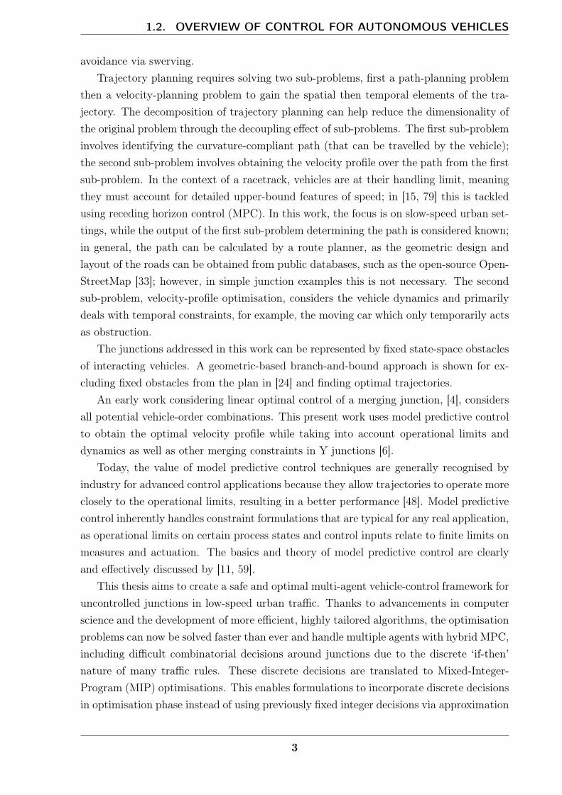
avoidance via swerving.Trajectory planning requires solving two sub-problems, first a path-planning problem
then a velocity-planning problem to gain the spatial then temporal elements of the tra-jectory. The decomposition of trajectory planning can help reduce the dimensionality ofthe original problem through the decoupling effect of sub-problems. The first sub-probleminvolves identifying the curvature-compliant path (that can be travelled by the vehicle);the second sub-problem involves obtaining the velocity profile over the path from the firstsub-problem. In the context of a racetrack, vehicles are at their handling limit, meaningthey must account for detailed upper-bound features of speed; in [15, 79] this is tackledusing receding horizon control (MPC). In this work, the focus is on slow-speed urban set-tings, while the output of the first sub-problem determining the path is considered known;in general, the path can be calculated by a route planner, as the geometric design andlayout of the roads can be obtained from public databases, such as the open-source Open-StreetMap [33]; however, in simple junction examples this is not necessary. The secondsub-problem, velocity-profile optimisation, considers the vehicle dynamics and primarilydeals with temporal constraints, for example, the moving car which only temporarily actsas obstruction.
The junctions addressed in this work can be represented by fixed state-space obstaclesof interacting vehicles. A geometric-based branch-and-bound approach is shown for ex-cluding fixed obstacles from the plan in [24] and finding optimal trajectories.
An early work considering linear optimal control of a merging junction, [4], considersall potential vehicle-order combinations. This present work uses model predictive controlto obtain the optimal velocity profile while taking into account operational limits anddynamics as well as other merging constraints in Y junctions [6].
Today, the value of model predictive control techniques are generally recognised byindustry for advanced control applications because they allow trajectories to operate moreclosely to the operational limits, resulting in a better performance [48]. Model predictivecontrol inherently handles constraint formulations that are typical for any real application,as operational limits on certain process states and control inputs relate to finite limits onmeasures and actuation. The basics and theory of model predictive control are clearlyand effectively discussed by [11, 59].
This thesis aims to create a safe and optimal multi-agent vehicle-control framework foruncontrolled junctions in low-speed urban traffic. Thanks to advancements in computerscience and the development of more efficient, highly tailored algorithms, the optimisationproblems can now be solved faster than ever and handle multiple agents with hybrid MPC,including difficult combinatorial decisions around junctions due to the discrete ‘if-then’nature of many traffic rules. These discrete decisions are translated to Mixed-Integer-Program (MIP) optimisations. This enables formulations to incorporate discrete decisionsin optimisation phase instead of using previously fixed integer decisions via approximation
3
CHAPTER 1. INTRODUCTION
or heuristics. The key elements discussed in this work are safety constraints, objectivefunctions, multi-agent simulations, and performance and scaling considerations. Examplesare based primarily around the simple atomic actions at uncontrolled junctions, such asmerging at Y junctions, and crossing cross and box junctions commonly found in urbanareas.
This work incorporates the order of vehicles merging or passing through an intersec-tion into an optimisation through mixed-integer programming and big-M relaxation. Forcontrol purposes, [61] shows Mixed-Integer Linear Programming (MILP) with MPC tocontrol a robotic agent.
Similar hybrid MPC formulations can consider discontinuous actuations, such as thethrottle and brake actions in vehicle control [47].
Optimisation- and MPC-related works appear in junction vehicle control schemes [51].The survey in [65] introduces related works involving intersections and merging junctions.
Alternatively, junction-control works can be based on time-space reservation algorithms.Dresner and Stone [22] detail an early reservation-based intersection-coordination policyin which the vehicles attempt to reserve grid tiles in the junction, which only one vehiclecan occupy at any given time; the intersection node decides if the reservation is accep-ted or rejected based on simulations. [20] demonstrates a reservation-based algorithm inwhich only the first vehicle can request a reservation and arrival time and must cross thejunction at full speed.
In [85], the authors develop an optimisation-based decentralised framework with aFirst-Come-First-Served (FCFS) policy. They implement approximate entry- and exit-time separation for vehicles in the junction area and show a trade-off between the fuelconsumption and congestion level of two connected intersections. Similarly, [64] shows anoptimisation-based framework with a FCFS policy and the same occupancy separationconstraints for merging on highway on-ramps.
Threat-assessment techniques are surveyed in [17] for collision avoidance. Kamal et al.[39] detail a risk-function-based MPC framework that minimises speed errors and accel-erations to avoid the risk of cross collision during intersection coordination.
A robust MPC scheme was proposed by [13] with a backup safety mode to abortthe mission in a safe way in case of conflict; however, another controller is needed torestart the vehicle from the safety mode. Rizaldi and Althoff [66] list safety-rule con-siderations for vehicles to make them accountable for their road cooperation affectingactions. Junction safety in [43, 44] is shown with MPC formulations, where an infinitehorizon contingency plan exists for the vehicles to maintain safety; additionally multiplevehicle ordering policies are detailed: rule based, FCFS, and concurrent crossing to fixthe crossing orders.
Some closely related works employ mixed-integer formulations similarly to this thesis.Qian et al. [58] show a relative-priority-based MPC approach utilising brake-safe sets to
4

1.3. STRUCTURE OF THE DISSERTATION
keep vehicles at safe distances from one another once their junction crossing order (rel-ative priority) has been heuristically determined and fixed. This relative-priority basedframework builds on the work [31] with results on acyclic priority graphs and traject-ory planning around junction obstacles of vehicle pairs. Altche et al. [2] uses MILP toevaluate similar junction-related obstacles in 2D configuration spaces seeking minimal-time control of vehicles passing through junction areas. In another highly relevant work,Altche et al. [3] detail a state-of-the-art branch-and-bound optimisation of Mixed-IntegerQuadratic Program (MIQP) implemented for semi-autonomous driving for the first time.Their work applies cooperative supervised vehicle control in junctions where the junctioncrossings orders (priorities) are not chosen heuristically but incorporated in the MIQPoptimisation with integer-programming tools. These relevant methods of the above au-thors are available in more detail in thesis works [1, 57]. A two-stage MPC approach in[5] shows a non-convex operating-region optimisation using simulated annealing to selectconvex obstacle-free regions, that later, in the second stage, used by a convex fast MPCfor safe robotic obstacle avoidance. This two-stage optimisation method was examined forthe vehicle-ordering problem being discussed in this paper, but was found to be limitedin its ability to handle a high number of vehicle-interaction hyperplanes.
In comparison, this thesis proposes a framework with a time-headway safety design,that has the collision sets inflated proportionally to the speed to achieve appropriate safetyclearances during junction crossing. Furthermore, it incorporates integrated decision mak-ing for the vehicle ordering problem within the Mixed-Integer Model Predictive Control(MI-MPC), allowing the framework to obtain globally-optimal vehicle orders and controlinputs at the same time instead of operating on some previously fixed orderings (frompriority fixing approaches). Robustness of the control time delay and information propaga-tion was addressed by forming spatio-temporal corner-cutting prevention constraints, asshown in [63]. Framework elements were tested with multiple cost formulations, policies,and additional junction-passing features; simplifications and added redundant constraintswere included to increase computational performance. Finally, the control was refor-mulated in a decentralised manner for cases with restricted perception and informationexchange.
1.3 Structure of the dissertation
Chapter 2 introduces the building blocks of the mixed-integer control framework. Start-ing with the route model and vehicle dynamics, time-headway safety considerations areintroduced in the form of the positive control invariant set with respect to temporarilyfixed road obstacles. The recursive feasibility of the MPC framework is shown to beclosely related to vehicle safety and collision avoidance. The framework is designed withsafety considerations to accommodate sudden stopping events of moving vehicles, achiev-
5

CHAPTER 1. INTRODUCTION
ing robustness against worst-case events, such as low-speed accidents. The design stepsare demonstrated in an example of Y-junction merging, where the safety constraints aretreated with the hyperplane formulation. Finally, the MI-MPC is formulated by employ-ing big-M relaxation and separating hyperplane theorem. Soft priorities are shown inthe decision-making process with relative weightings; examples of cooperation behavioursbetween vehicles are provided.
Chapter 3 discusses two formulations of the convex quadratic cost functions, showing aclose connection between them. For intended operational cases, the two formulations areshown to result in equivalent optimisations and solution trajectories under given tuningconditions. The tuning of cost-weight parameters is designed with Linear QuadraticRegulator (LQR) theory in relation to the time-headway parameter yielding inherentstability results for single-agent cases. The characteristic that governs how vehicles slowdown near obstacles is investigated in relation of time-headway parameter and horizon-length choices. An additional cost element is introduced for soft pre-avoidance to provideapproximate early reactions to junction decisions (obstacles); its effect is shown on a pairof vehicles approaching a Y junction and merging. Finally, in the case of varying upper-and lower-bound speeds (e.g. around junctions, and at speed bumps), the MIP relaxationis shown with safe corner-cutting prevention.
In Chapter 4, the simulations are expanded to multi-agent vehicle-control cases forcross junctions. Examples are shown for a fixed number of vehicles looping within thejunction simulations on double-O loops and 8-shaped loops. The potential for deadlockscenarios in these junctions due to their structural properties is discussed and displayed.A deadlock-free modification is then introduced in box junctions by extending the MIPframework. Various policies are then compared, those being a simple FCFS heuristicpolicy, the designed hybrid MPC, and the extended soft pre-avoidance early-reactionpolicy.
Chapter 5 examines performance-improvement methods for the cross-junction problemfrom Chapter 4. The problem can be changed to a simpler form, on account of theorthogonality between shared vehicle-interaction constraints, by removing the redundanthyperplanes. Two different approaches are explored in attempt to increase the speed ofoptimisation by adding redundant binary constraints. Finally, decentralised policies areformulated using sequentially shared future plans; trajectory densities accompany thegiven formulations for comparison.
Chapter 6 provides concluding remarks as well as potential future research directionsthat have emerged as a result of this thesis.
Supplementary material, result tables and notes are provided in the appendices.
6

1.5. ACRONYMS
1.4 Notations
This section provides a list of common notations that are used throughout this workalongside clarifying descriptions of respective definitions. Disambiguating comments areincluded where a single notation has multiple meanings and the context does not offerclear certainty. For example, notations in control theory and traffic analysis overlap inthe case of Q which is used for both the quadratic cost matrix and traffic flow measure.
Z Integer numbersR Real numbersx Vector, (e.g. x ∈ Rn real valued vector of size n, x = [xi, i = 1, . . . , n])x Or concatenated decision vector, (e.g. x = [xn, n = 1, . . . , N ], where a state vector is
xn for the agent index n aggregated for compactness in multi-agent problems)X Matrix, (X ∈ Rn×m real valued matrix of size n×m)T Transpose, T in superscriptδt Control period time, unit in seconds: [s]t Continuous time, unit in seconds: [s]tk Discrete time at k index tk := kδt, unit in seconds: [s][x, y] = r(t) Position vector of a particle at time t in 2D Cartesian coordinates, unit in [m]
s Arc length, one-dimensional position, measured along the path, unit in [m]
[x, y] = r(s) Map of arc length to 2D Cartesian coordinates, unit in [m]
J Scalar cost (performance index)∗ Optimal value (e.g. J∗ optimal cost)q, r, Q, R Scalar and matrix weights in cost functions for quadratic states and control inputsqf, Qf Scalar and matrix weights of terminal states
Q, ρ In traffic analysis, scalar measures of traffic flow Q
[vehh
]and density ρ
[vehkm
]p, q or a, b General vehicle indices commonly used in parameter or variable subscripts., . Set of two or more elements (e.g. p, q a set of two vehicle indices)(., .) Ordered set of two or more elements (e.g. (p, q) two vehicles with car-following order)Np Prediction horizon lengthmin, max Minimum and maximum value of a parameter or variable, in subscriptX Allowed state set, x ∈ X , commonly speed limits X = s, v | vmin ≤ v ≤ vmaxU Allowed control set, u ∈ U , commonly acceleration limits U = u | amin ≤ u ≤ amax
1.5 Acronyms
MPC Model Predictive ControlMIP Mixed-Integer ProgramMI-MPC Mixed-Integer Model Predictive ControlMILP Mixed-Integer Linear ProgramMIQP Mixed-Integer Quadratic ProgramLTI Linear Time InvariantLQR Linear Quadratic RegulatorFCFS First-Come-First-Served
7

8
2Vehicular control with time-headway
MI-MPC
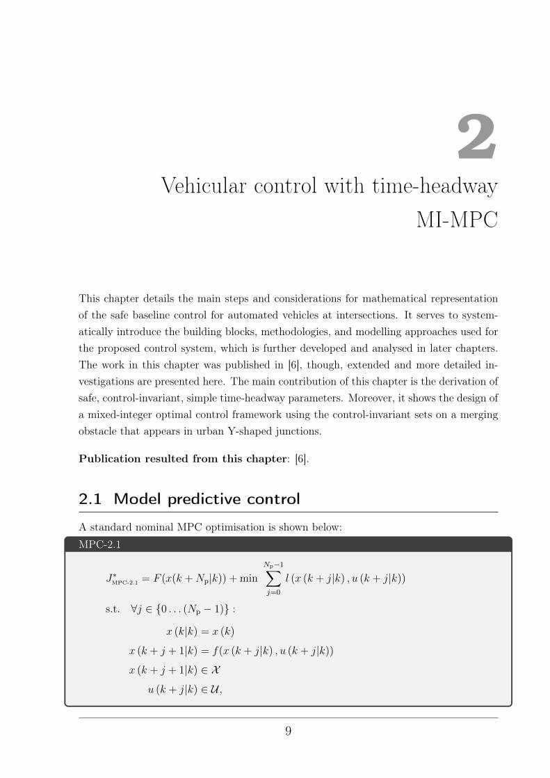
This chapter details the main steps and considerations for mathematical representationof the safe baseline control for automated vehicles at intersections. It serves to system-atically introduce the building blocks, methodologies, and modelling approaches used forthe proposed control system, which is further developed and analysed in later chapters.The work in this chapter was published in [6], though, extended and more detailed in-vestigations are presented here. The main contribution of this chapter is the derivation ofsafe, control-invariant, simple time-headway parameters. Moreover, it shows the design ofa mixed-integer optimal control framework using the control-invariant sets on a mergingobstacle that appears in urban Y-shaped junctions.
Publication resulted from this chapter: [6].
2.1 Model predictive control
A standard nominal MPC optimisation is shown below:MPC-2.1
J∗MPC-2.1 = F (x(k +Np|k)) + min
Np−1∑j=0
l (x (k + j|k) , u (k + j|k))
s.t. ∀j ∈ 0 . . . (Np − 1) :
x (k|k) = x (k)
x (k + j + 1|k) = f(x (k + j|k) , u (k + j|k))
x (k + j + 1|k) ∈ X
u (k + j|k) ∈ U ,
9
CHAPTER 2. VEHICULAR CONTROL WITH TIME-HEADWAY MI-MPC
where the state and control inputs are x and u, respectively; the cost function, J , isminimised and consists of the summation of stage costs l(x, u) and the terminal costF (x); control times are at tk = t(k) := kδt, where the discrete time is k ∈ Z and thepositive sampling or period time is δt; process dynamics are defined by the discretisedmodel x(k + 1) = f(x(k), u(k)) while x ∈ X and u ∈ U , where the allowed state andcontrol sets are X and U , respectively.
2.2 Problem definition
The aim is to tackle vehicle-control problems for a set of N = 1, 2, . . . , N digitally con-trolled vehicles (e.g. automated or autonomous cars). Urban traffic environments wereselected where the fixed road-network layout is known and vehicle interactions happenat relatively slow speeds (< 10 ms−1), with focus on uncontrolled and non-signalisedjunctions. Low traffic speeds provide more time for decision-making in the control op-timisation while the relatively high vehicle density on roads gives way to more vehicleinteractions and non-trivial, intricate situations. The simple safety approach developedin this work is based on time-headway separation; this separation approach is valid primar-ily for low-speed environments; it becomes inefficient in high-speed traffic due to longerthan necessary inter-vehicle separation gaps. Other model simplifications serve to neg-lect quadratic speed-dependent terms in vehicle dynamics, such as air drag and lateraldynamics on curved paths (assuming curvature-compliant, reasonably planned paths).Specific characteristic dynamics may appear when driving slower than a rolling stop, suchas probabilistic stopping, which is a sudden-stop event at near zero speed. Unmodelledfriction terms and tribological properties are responsible for probabilistic stopping whichpresent through the drivetrain and during tire-pavement contact. Sudden-stop events, aswith probabilistic stopping, occur when a vehicle experiences an unexpected state evolu-tion and abruptly decelerates from rolling to a stationary state. In a worst-case scenario,this could be an accident or other non-operational emergency situations ahead of the con-trolled vehicle, necessitating a safe response. Nominal MPC with hard output constraintslike obstacle or collision avoidance may easily become infeasible in the presence of suddenstop events or other model mismatch errors. The rate of model mismatch grows alongsidethe number of simplifications and assumptions common at higher levels of abstractionwhere also longer control period times are dominant; this is a practical rule for high levelcontrollers in the control hierarchy, usually considering slowly changing model dynamicsover a longer period of time [69].
The applied MPC approach is designed as a mid- to high-level controller that tacklesrelatively slow (1–10 s) mission-specific trajectories. Lower, specialised controllers aredeveloped to accept reference controls and trajectories from the MPC [69]; moreover,they serve to handle unmodelled, high-frequency dynamics, such as the engine, braking,
10
2.2. PROBLEM DEFINITION
steering and suspension control. These are exempt from modelling due to their frequency,complexity and moderate influence on the modelled time scale.
For describing and controlling vehicles, vehicle motion is calculated in a simplifiedapproach for a single particle representing a vehicle as a point-mass. The function ofposition coordinates (position vector) r(t) is to describe the 2D spatial position vector ofthe vehicle particle on the Cartesian plane at a given time t (or, if terrain is involved, in3D space); thus, the motion of the particle is considered known:[
x
y
]= r(t) ∈ R2. (2.2)
A possible decomposition of the motion into two sub-elements is based on the determina-tion of its graph (the path) and the travel plan along this path. The path is a time-orderedset of coordinates for particle positions. It is worth noting that the path alone does notdefine the motion, as it is missing the temporal element of the motion.
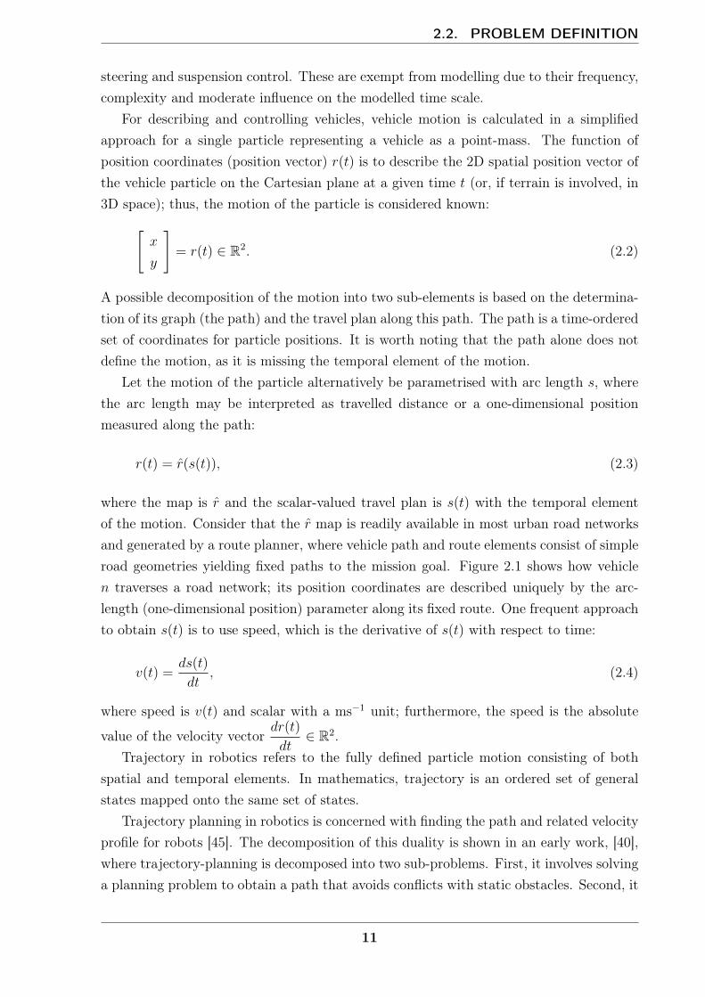
Let the motion of the particle alternatively be parametrised with arc length s, wherethe arc length may be interpreted as travelled distance or a one-dimensional positionmeasured along the path:
r(t) = r(s(t)), (2.3)
where the map is r and the scalar-valued travel plan is s(t) with the temporal elementof the motion. Consider that the r map is readily available in most urban road networksand generated by a route planner, where vehicle path and route elements consist of simpleroad geometries yielding fixed paths to the mission goal. Figure 2.1 shows how vehiclen traverses a road network; its position coordinates are described uniquely by the arc-length (one-dimensional position) parameter along its fixed route. One frequent approachto obtain s(t) is to use speed, which is the derivative of s(t) with respect to time:
v(t) =ds(t)
dt, (2.4)
where speed is v(t) and scalar with a ms−1 unit; furthermore, the speed is the absolute
value of the velocity vectordr(t)
dt∈ R2.
Trajectory in robotics refers to the fully defined particle motion consisting of bothspatial and temporal elements. In mathematics, trajectory is an ordered set of generalstates mapped onto the same set of states.
Trajectory planning in robotics is concerned with finding the path and related velocityprofile for robots [45]. The decomposition of this duality is shown in an early work, [40],where trajectory-planning is decomposed into two sub-problems. First, it involves solvinga planning problem to obtain a path that avoids conflicts with static obstacles. Second, it
11

CHAPTER 2. VEHICULAR CONTROL WITH TIME-HEADWAY MI-MPC
Figure 2.1: Vehicle route from A to B over the road network (with position definitions).
involves solving a velocity-planning problem, to describe the motion over the fixed pathfrom the first step, to avoid conflicts with temporary, moving obstacles that could imposeconflicting states at certain time intervals. In [15, 79], semi-analytical velocity-profile-optimisation problems are shown with MPC (receding horizon control) formulation alongthe fixed path of racetracks.
Fixed paths in urban environments are obtained using a mission or route planner.These paths are planned between the starting (current) position and the destinationposition (Figure 2.1). The path-planning that calculates the fixed path (r map) is notconsidered further in this work; the path is instead treated as a known, since examplesmaking use of it are simplistic to the point of triviality (e.g. traversing on a one-way road).However, the path is assumed to be feasible in respect of vehicle kinematics, operationallimits, and lateral accelerations (e.g. curvature compliant with respect to corner geometriesand permanently static features, such as pavement shape or parked vehicles). When thepath is not feasible, it is not guaranteed that the mission goal of the vehicle would bereached in a finite time without replanning the path.
s(t) arc length parametrisation can be linearly transformed, without loss of generality(e.g. arbitrarily shifted and scaled to obtain a generalised position parameter). In thiswork, s is simply referred to as position, with the default unit in meters [m] and will be shif-ted to arbitrarily place the origin at the junction of interest. In multi-degree-of-freedom ro-botic systems, the number of general positions (N) describes application-specific measures,joint degrees, linear positions, etc., which lead to an intuitive N -dimensional coordination-space representation. Within this coordination space, interference between coordinates,such as robotic arm links, are represented as obstacles, as shown in [72].
The N -dimensional general position space in a traffic system describes agent positionsfor each considered vehicle. Additionally, 2D pairwise vehicle-coordination planes [45] canbe used to represent unwanted vehicle-interference positions (e.g. collision of finite vehiclebodies); see [30, 31, 58] where the obstacles are convex approximations of the real con-flicting positions. The configuration space for three vehicles is shown in Figure 2.2, withthe grey obstacle bodies representing convexified collision sets. Alternatively, normalisedspace representation appears in the literature, where s is defined over [0, 1] range, which
12
2.2. PROBLEM DEFINITION
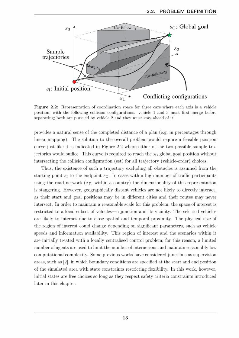
Figure 2.2: Representation of coordination space for three cars where each axis is a vehicleposition, with the following collision configurations: vehicle 1 and 3 must first merge beforeseparating; both are pursued by vehicle 2 and they must stay ahead of it.
provides a natural sense of the completed distance of a plan (e.g. in percentages throughlinear mapping). The solution to the overall problem would require a feasible positioncurve just like it is indicated in Figure 2.2 where either of the two possible sample tra-jectories would suffice. This curve is required to reach the sG global goal position withoutintersecting the collision configuration (set) for all trajectory (vehicle-order) choices.
Thus, the existence of such a trajectory excluding all obstacles is assumed from thestarting point sI to the endpoint sG. In cases with a high number of traffic participantsusing the road network (e.g. within a country) the dimensionality of this representationis staggering. However, geographically distant vehicles are not likely to directly interact,as their start and goal positions may be in different cities and their routes may neverintersect. In order to maintain a reasonable scale for this problem, the space of interest isrestricted to a local subset of vehicles—a junction and its vicinity. The selected vehiclesare likely to interact due to close spatial and temporal proximity. The physical size ofthe region of interest could change depending on significant parameters, such as vehiclespeeds and information availability. This region of interest and the scenarios within itare initially treated with a locally centralised control problem; for this reason, a limitednumber of agents are used to limit the number of interactions and maintain reasonably lowcomputational complexity. Some previous works have considered junctions as supervisionareas, such as [2], in which boundary conditions are specified at the start and end positionof the simulated area with state constraints restricting flexibility. In this work, however,initial states are free choices so long as they respect safety criteria constraints introducedlater in this chapter.
13
CHAPTER 2. VEHICULAR CONTROL WITH TIME-HEADWAY MI-MPC
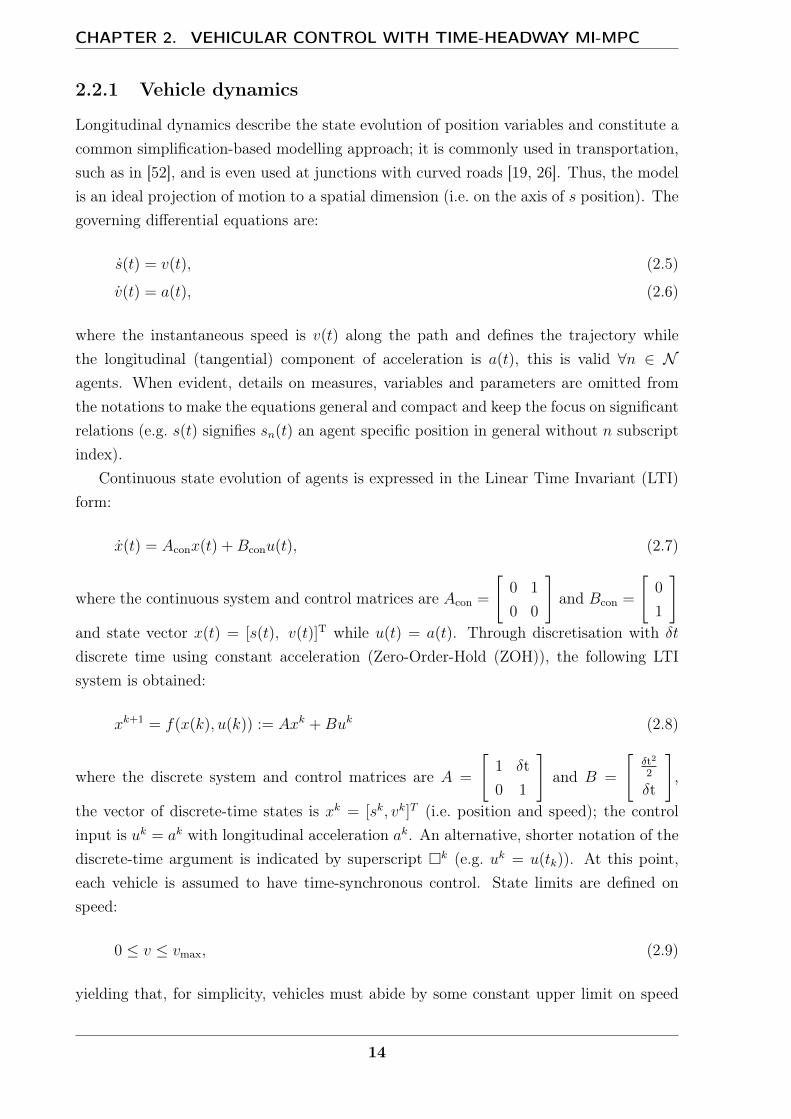
2.2.1 Vehicle dynamics
Longitudinal dynamics describe the state evolution of position variables and constitute acommon simplification-based modelling approach; it is commonly used in transportation,such as in [52], and is even used at junctions with curved roads [19, 26]. Thus, the modelis an ideal projection of motion to a spatial dimension (i.e. on the axis of s position). Thegoverning differential equations are:
s(t) = v(t), (2.5)
v(t) = a(t), (2.6)
where the instantaneous speed is v(t) along the path and defines the trajectory whilethe longitudinal (tangential) component of acceleration is a(t), this is valid ∀n ∈ Nagents. When evident, details on measures, variables and parameters are omitted fromthe notations to make the equations general and compact and keep the focus on significantrelations (e.g. s(t) signifies sn(t) an agent specific position in general without n subscriptindex).
Continuous state evolution of agents is expressed in the Linear Time Invariant (LTI)form:
x(t) = Aconx(t) +Bconu(t), (2.7)
where the continuous system and control matrices are Acon =
[0 1
0 0
]and Bcon =
[0
1
]and state vector x(t) = [s(t), v(t)]T while u(t) = a(t). Through discretisation with δt
discrete time using constant acceleration (Zero-Order-Hold (ZOH)), the following LTIsystem is obtained:
xk+1 = f(x(k), u(k)) := Axk +Buk (2.8)
where the discrete system and control matrices are A =
[1 δt0 1
]and B =
[δt22
δt
],
the vector of discrete-time states is xk = [sk, vk]T (i.e. position and speed); the controlinput is uk = ak with longitudinal acceleration ak. An alternative, shorter notation of thediscrete-time argument is indicated by superscript k (e.g. uk = u(tk)). At this point,each vehicle is assumed to have time-synchronous control. State limits are defined onspeed:
0 ≤ v ≤ vmax, (2.9)
yielding that, for simplicity, vehicles must abide by some constant upper limit on speed
14

2.3. OBSTACLE HANDLING
and are part of uni-directional traffic, meaning they cannot move backwards on their path.Limitations in lateral dynamics may drive variations in the upper bounds of speed, whichis important for race cars on curvilinear tracks or minimal-time velocity optimisation,as in [15]. However, the scenarios being discussed are in low-speed urban environments,meaning there is no real need to drive at the physical limits of the vehicle—lateral dynam-ics constitute less of a dominant factor in these situations. The speed limits are respectedin t ∈ [tk, tk+1] by defining (2.9) at both the start and end of the single control period(i.e. tk and tk+1). This is evident, as the continuous-time speed function v(t) is linearon t ∈ [tk, tk+1] because the LTI (2.8) with constant acceleration (ZOH) and the integralrelation from (2.6) result in a line segment. Thus, the full line segment remains withinthe speed limits, since the points on this line segment (inter-sample speeds) are the linearcombination of its extrema. Moreover, simple dynamics constraints are assumed, such as:
Fmax bra ≤ F ≤ Fmax tra, (2.10)
where the longitudinal force is F , which acts on the vehicle; the maximum braking forcelimit is Fmax bra; the maximum tractor force limit is Fmax tra. Through simplification withthe non-changing mass of vehicle, the acceleration limits are:
amin ≤ a ≤ amax, (2.11)
where the maximum deceleration is amin < 0 (lower limit on acceleration) and the max-imum acceleration limit is amax > 0.
As a result of the deterministic vehicle model, new state predictions can be madewith (2.8) simply as equality constraints; moreover, (2.9) and (2.11) provide inequal-ity constraints for simple speed and acceleration limits. These are readily incorpor-ated in X and U sets in MPC 2.1 optimisation as X = s, v | vmin ≤ v ≤ vmax andU = u | amin ≤ u ≤ amax or could be imposed as part of the linear matrix inequalities.The following section discusses the construction of safety sets and constraints for variousvehicle interactions.
2.3 Obstacle handling
Stationary and static obstacles, such as road features and parked vehicles, are included inthe fixed-path plan and are known in the problem. Thus, obstacle avoidance in the velocityoptimisation is concerned with moving or mobile obstacles at certain locations at certaintimes, such as other vehicles on the roads and in junctions. As previously discussed,the complete trajectory plan is determined once the velocity optimisation is solved andfeasible. Following the approximated obstacle formulation of [30], convex collision sets
15

CHAPTER 2. VEHICULAR CONTROL WITH TIME-HEADWAY MI-MPC
Figure 2.3: Schematic of a two-car merging scenario; s1, s2 are positions along route. [6]
Figure 2.4: Cpq collision set indicated for two merging vehicles. [6]
are defined around the undesirable positions of each conflicting vehicle pair p, q ∈ Nsuch that p 6= q. This set of positions includes those where the vehicle body frames wouldoverlap, indicating physical contact and collision. Without a loss of generality, the interestis initially a single merging, as shown in Figure 2.3. Consequently, the convex boundingcollision set of a merging interaction is a single joint polyhedron defined as:
Cpq := xp, xq|sp > L1, sq > L2, sp − sq > L3, sq − sp > L4, (2.12)
where constants Li, i = 1, . . . 4 determine the shape and position1 of the mergingobstacle over the sp–sq 2D configuration plane (see Figure 2.4).
Pairwise vehicle conflict is defined as:
Cpq 6= ∅, (2.13)
and the collision with this obstacle is defined as:
[xp, xq] ∈ Cpq. (2.14)1For the merging obstacle without loss of generality, the constants incorporate the position offsets
L1 := soffp − l1pq, L2 := soffq − l2pq, L3 := soffp − soffq − l1pq, L4 := soffq − soffp − l2pq (shown in Figure 2.4).
16

2.3. OBSTACLE HANDLING
Hence, the imposed constraint for the vehicle states are:
[xp, xq] /∈ Cpq (2.15)
or, alternatively:
[xp, xq] ∈ Cpq, (2.16)
where the complement of C is C.Recursive feasibility and vehicle safety are strongly related to collision-free vehicle
control where invariant set theory is employed to obtain theoretical guarantees.
2.3.1 Invariant sets
The recursive feasibility property is essential for safety-critical optimisation problems, inwhich guaranteed constraint satisfaction must be ensured at all costs [42]. The proposedframework considers safety constraints to ensure vehicle separation from obstacles andfrom other vehicles with (2.16).
Following the definition from [42] for a discrete time system xk+1 = f(xk, uk):
Ω is control invariant⇔ ∀x ∈ Ω, ∃u ∈ U such f(x, u) ∈ Ω. (2.17)
For simplicity, the vehicle in consideration must remain in the set of safe states to be ableto stop before a static obstacle position (e.g. the goal position, a junction entry, or behindanother (temporarily) stationary vehicle).
2.3.2 Headway
As a preliminary to constructing the safe invariant set, spatial and temporal measures forthe distance between vehicles are introduced.
The spatial distance, ‘distance headway’, is the distance between the correspondingreference points of two vehicles following each other at a given time assuming the samevehicular paths. Thus, dh(t) = sl(t)− sf(t), where the longitudinal positions on the roadfor the leader vehicle is sl and, for the follower vehicle, is sf. The leader vehicle is, bydefinition, ahead of the follower; thus, dh > 0. The distance gap measure, or simply thegap, is the clearance between vehicles defined as dg(t) = sl(t)−Ll−sf(t), where the leadervehicle length is Ll and the vehicle reference points are at the front bumpers; the positivegap or clearance dg > 0 is a stricter constraint assuming finite length vehicle bodies.
The temporal distance, time headway, is the temporal counterpart of ‘distance head-way’; it is similarly used as a method of analysis for interpreting traffic-flow data [75].Gross time headway, is measured between the corresponding points of vehicles reaching
17
CHAPTER 2. VEHICULAR CONTROL WITH TIME-HEADWAY MI-MPC
the same position on the road (i.e. tgh = tf − tl, sf(tf) = sl(tl)). Net time headway, or thetime gap, is the time span between the front bumper of the follower vehicle reaching theposition of the rear bumper of the leader vehicle (i.e. tnh = tf − tl, sf(tf) = sl(tl) − Ll).As traffic-flow analysis is done on time-space diagrams of existing vehicle-trajectory data,the headway measures are relatively straightforward to read off of the graphs on thecorresponding axes (i.e. t-time and s-space).
However, real-time control cannot readily ascertain the current gross or net time head-way between vehicles without making additional assumptions to predict future vehiclebehaviours and trajectories. This inherently causes a prediction error in the measure, asin general predictions may differ from the course of real events and states.
In this thesis, ‘time headway’ is used to refer to the similar concept of net time headway,or the time gap, between the controlled (follower) vehicle and the worst-case assumptionof the leader’s rear-bumper position interpreted as a stationary obstacle. This relates tothe conservative approach of worst-case dynamics for instantaneous stops of the leadervehicles. It is a cautious approach, as the capabilities and actions of the leader vehiclesare not necessarily known in advance by the follower vehicles. Thus, in this work, timeheadway th is a worst-case vehicle-specific parameter, rather than a data-analysis tool forpost-processing. The th parameter will be extensively used in this work to ensure safeclearances and prevent collisions.
2.3.3 Simple time-headway invariant set
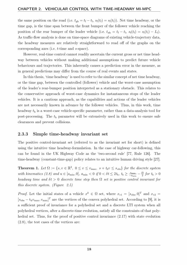
The positive control-invariant set (referred to as the invariant set for short) is definedusing the intuitive time headway-formulation. In the case of highway car-following, thiscan be found in the UK Highway Code as the ‘two-second rule’ [77, Rule 126]. Thetime-headway (constant-time-gap) policy relates to an intuitive human driving style [27].
Theorem 1. Let Ω := s, v ∈ R2, 0 ≤ v ≤ vmax, s + thv ≤ sobs for the discrete systemwith kinematics (2.8) and u ∈ [amin, 0], amin < 0 if 0 < δt ≤ 2th, th ≥ vmax
−amin− δt
2for th > 0
headway time and δt > 0 discrete time step then Ω set is positive control invariant forthis discrete system. (Figure 2.5)
Proof. Let the initial states of a vehicle xk ∈ Ω set, where xv1 = [sobs, 0]T and xv2 =
[sobs − thvmax, vmax]T are the vertices of the convex polyhedral set. According to [9], it is
a sufficient proof of invariance for a polyhedral set and a discrete LTI system when allpolyhedral vertices, after a discrete-time evolution, satisfy all the constraints of that poly-hedral set. Thus, for the proof of positive control invariance (2.17) with state evolution(2.8), the test cases of the vertices are:
18
2.3. OBSTACLE HANDLING
Vertex v1: xk = xv1 = [sobs, 0]T
sk+1 =sobs +1
2akδt2, (2.18)
vk+1 =akδt, (2.19)
for the trivial solution of ak = 0 the states remain unchanged, satisfying xk+1 ∈ Ω.Vertex v2: xk = xv2 = [sobs − thvmax, vmax]
T
sk+1 =sobs − thvmax + vmaxδt +1
2akδt2, (2.20)
vk+1 =vmax + akδt. (2.21)
The new states must satisfy each of the constraints defining Ω. Inequality 0 ≤ vk+1 from(2.9) combined with (2.21) yields:
δt ≤ vmax
−ak, for ak < 0. (2.22)
The constraint of vk+1 ≤ vmax from (2.9) with (2.21) is satisfied for ak ≤ 0 control choice.The final constraint gives:
sk+1 + thvk+1 ≤ sobs. (2.23)
Using (2.20), (2.21) and (2.23):
vmax + ak(
1
2δt + th
)≤ 0 (2.24)
by substituting the maximum available deceleration (minimum acceleration):
vmax
−amin
≤ 1
2δt + th. (2.25)
Moreover, by combining (2.22) and (2.24), they give:
vmax + ak(
1
2δt + th
)≤ 0 ≤ vmax + akδt, (2.26)
δt ≤ 2th, (2.27)
for ak < 0.
In Figure 2.6, th–δt parameter regions are shown where Ω set is a positive control-invariant using (2.25) and (2.27).
Remark: Ω can be closed by another side from the left (assuming safe non-emptyset (i.e. sc < sobs)) at arbitrary sc < sk, resulting in two more vertices (xv3 = [sc, 0]T ,
19

CHAPTER 2. VEHICULAR CONTROL WITH TIME-HEADWAY MI-MPC
Figure 2.5: Shaded area represents the Ω set. [6]
Figure 2.6: The shaded region indicates th–δt parameter choices that ensure Ω set to be apositive control-invariant set. [6]
xv4 = [sc, vmax]T ) if sc < sobs− thvmax or, otherwise, three vertices overall. However, these
instances are covered by the trivial solutions of previous case studies of vertices and bythe monotonic rule of sc < sk ≤ sk+1 ≤ sobs; thus, they can be disregarded from furtherproblem formulation.
A comparison between the introduced Ω invariant set is shown in Figure 2.7 againstthe maximal invariant set with the same vehicle properties. Both Ω sets with δt ≈ 0 and0.5 s were chosen with the minimal allowed th. The maximal invariant set was computediteratively using the dual of a one-step reachable set [11]:
Pre(S) , x ∈ Rn, ∃u ∈ U s.t. f (x, u) , (2.28)
where the initial S0 =
[0, 0]T
is the single rightmost corner point (i.e. the closest sta-tionary vehicle position). The maximal invariant set was iteratively calculated backwardswith:
Sk−1 = Pre(Sk) ∩ X , (2.29)
where the representation of the permitted speed range is incorporated in the X set.
20
2.3. OBSTACLE HANDLING
-30 -25 -20 -15 -10 -5 0
s [m]
0
2
4
6
8
10
12
v [
m/s
]
Ωdis
maximal Inv. set boundary
Ω boundary (δ t = 0.5 s)
Ω boundary (δ t = 0 s)
Continuous stopping before sobs
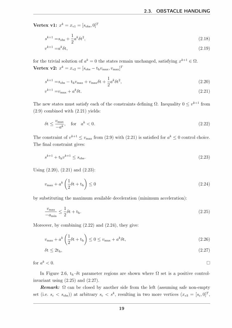
Figure 2.7: Comparison of discrete positive control-invariant sets generated with vmax =10 ms−1 , amin = −4.5 ms−2, sobs = 0, δt = 0.5 s ≤ −vmax/amin and δt = 0 s
Furthermore, Figure 2.7 illustrates the distance gap between the rightmost maximumspeed, vmax, of the Ω-invariant set and the continuous physical invariant stopping setincrease for higher speeds. This gap is the reason why simple time-headway models areacceptable for low-speed traffic and why, conversely, they are overly conservative for high-speeds; high-speed models must also consider higher order terms and tuned parameters toproperly describe the physical behaviours in wide range around the operating work-point:(i.e. desired speed).
2.3.3.1 Numerical example: Safe stop
In the following example, a vehicle approaches an obstacle at sobs = 50 m using an Ω
invariant set while satisfying (2.9) and (2.11) operational limits. The control is onlycalculated for a single time step ahead (Np = 1) in a reactive control fashion, maximisingthe speed.MPC-2.2
min |vmax − v (k + 1|k)|
s.t. :
x (k|k) = x (k)
x (k + 1|k) = A x (k|k) +B u (k|k)
x (k + 1|k) ∈ Ω
x ∈ X
u ∈ U
Notice the simple l1 norm objective function in control MPC 2.2, which has a connectionto the terminal position objective.
21

CHAPTER 2. VEHICULAR CONTROL WITH TIME-HEADWAY MI-MPC
0 10 20 30
k [-]
0
50
s [
m] obstacle position
vehicle position
0 10 20 30
k [-]
0
5
10v
[m
/s] v
max
speed
Figure 2.8: Simulation of one-step method with Ω and sobs = 50m obstacle.
Proposition 1. If the objective function J = |vmax − v (k + 1|k)| in MPC 2.2, then itresults in an equivalent optimisation using J ≡ −s (k + 1|k) as an objective function.
Proof. This is shown using the dynamics constraints that the optimisation is subject to
v (k + 1|k) = v(k) + a(k|k) δt, (2.31)
thus:
s (k + 1|k) = s(k) +1
2(v(k) + v (k + 1|k)) δt, (2.32)
resulting in:
J = |vmax − v (k + 1|k)| =∣∣∣∣vmax +
2
δt(s(k)− s(k + 1|k)) + v(k)
∣∣∣∣ . (2.33)
Furthermore, since the speed-operating region is 0 ≤ v ≤ vmax
J = |vmax − v (k + 1|k)| ≡ vmax − v (k + 1|k) ≥ 0, (2.34)
gives
J ≡ vmax +2
δt(s(k)− s(k + 1|k)) + v(k). (2.35)
where the only optimised decision variable is −s(k + 1|k), a position term; the rest areconstants resulting in mathematically equivalent optimisations subject to the originalconstraints.
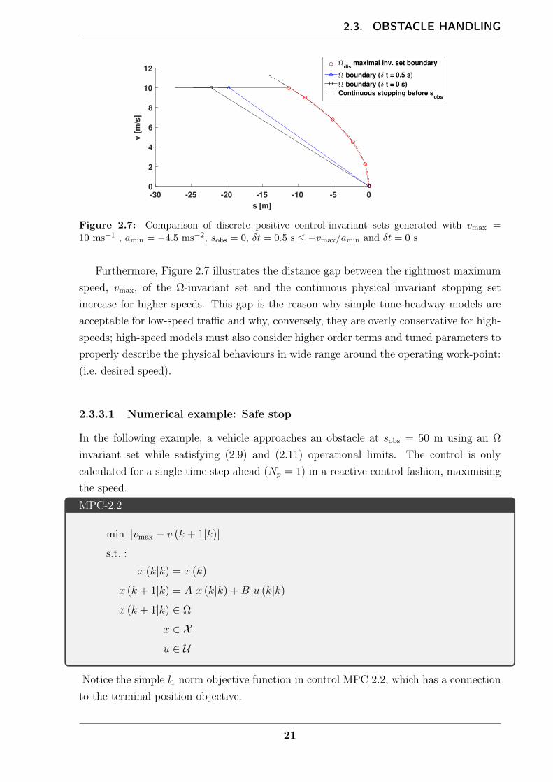
Figure 2.9 shows the v–s trajectory of Figure 2.8 with discrete states remaining withinthe bounds of Ω. In contrast, the continuous states can leave the set within an inter-sample
22
2.3. OBSTACLE HANDLING
0 10 20 30 40 50
s [m]
0
5
10
v [
m/s
]
Ω boundary
Continuous trajectory
Trajectory at discrete time
Figure 2.9: The v–s state trajectory in Ω-invariant set approaching a static obstacle.
period time but must return until the next discrete control time.A trivial, sufficient condition requires that the initial states of the control must satisfy
all constraints. In conclusion, the proposed control with Ω is recursively feasible forapproaching static obstacles with constraints on the first predicted time step.
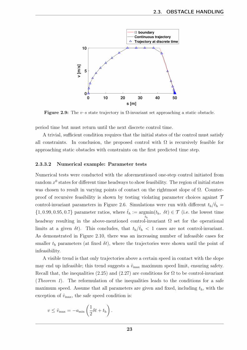
2.3.3.2 Numerical example: Parameter tests
Numerical tests were conducted with the aforementioned one-step control initiated fromrandom x0 states for different time headways to show feasibility. The region of initial stateswas chosen to result in varying points of contact on the rightmost slope of Ω. Counter-proof of recursive feasibility is shown by testing violating parameter choices against Tcontrol-invariant parameters in Figure 2.6. Simulations were run with different th/th =
1, 0.99, 0.95, 0.7 parameter ratios, where th := argminth
(th, δt) ∈ T (i.e. the lowest time
headway resulting in the above-mentioned control-invariant Ω set for the operationallimits at a given δt). This concludes, that th/th < 1 cases are not control-invariant.As demonstrated in Figure 2.10, there was an increasing number of infeasible cases forsmaller th parameters (at fixed δt), where the trajectories were shown until the point ofinfeasibility.
A visible trend is that only trajectories above a certain speed in contact with the slopemay end up infeasible; this trend suggests a vmax maximum speed limit, ensuring safety.Recall that, the inequalities (2.25) and (2.27) are conditions for Ω to be control-invariant(Theorem 1). The reformulation of the inequalities leads to the conditions for a safemaximum speed. Assume that all parameters are given and fixed, including th, with theexception of vmax, the safe speed condition is:
v ≤ vmax = −amin
(1
2δt+ th
).
23
CHAPTER 2. VEHICULAR CONTROL WITH TIME-HEADWAY MI-MPC
(a)0 10 20 30 40 50 60 70
s [m]
0
2
4
6
8
10
12
v [m
/s]
(b)0 10 20 30 40 50 60 70
s [m]
0
2
4
6
8
10
12
v [m
/s]
(c)0 10 20 30 40 50 60 70
s [m]
0
2
4
6
8
10
12
v [m
/s]
(d)0 10 20 30 40 50 60 70
s [m]
0
2
4
6
8
10
12
v [m
/s]
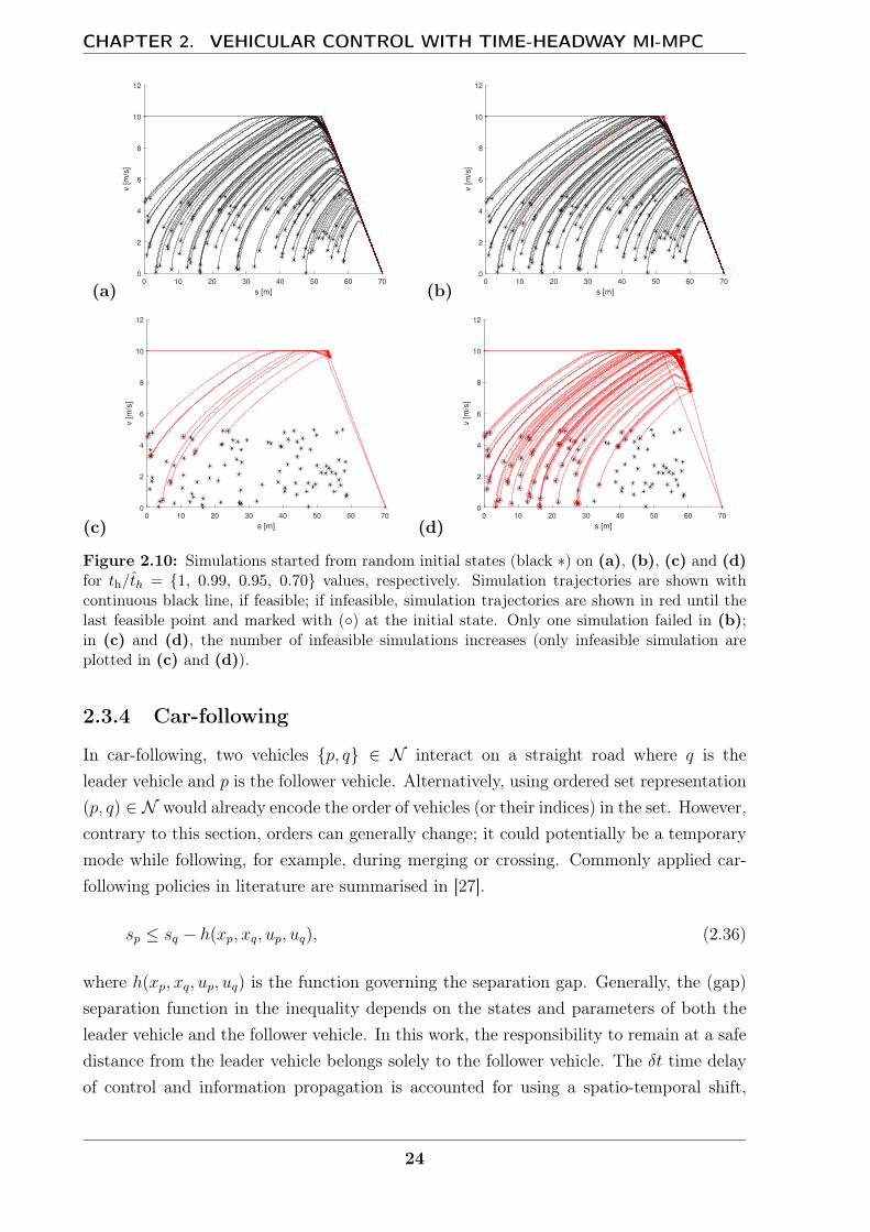
Figure 2.10: Simulations started from random initial states (black ∗) on (a), (b), (c) and (d)for th/th = 1, 0.99, 0.95, 0.70 values, respectively. Simulation trajectories are shown withcontinuous black line, if feasible; if infeasible, simulation trajectories are shown in red until thelast feasible point and marked with () at the initial state. Only one simulation failed in (b);in (c) and (d), the number of infeasible simulations increases (only infeasible simulation areplotted in (c) and (d)).
2.3.4 Car-following
In car-following, two vehicles p, q ∈ N interact on a straight road where q is theleader vehicle and p is the follower vehicle. Alternatively, using ordered set representation(p, q) ∈ N would already encode the order of vehicles (or their indices) in the set. However,contrary to this section, orders can generally change; it could potentially be a temporarymode while following, for example, during merging or crossing. Commonly applied car-following policies in literature are summarised in [27].
sp ≤ sq − h(xp, xq, up, uq), (2.36)
where h(xp, xq, up, uq) is the function governing the separation gap. Generally, the (gap)separation function in the inequality depends on the states and parameters of both theleader vehicle and the follower vehicle. In this work, the responsibility to remain at a safedistance from the leader vehicle belongs solely to the follower vehicle. The δt time delayof control and information propagation is accounted for using a spatio-temporal shift,
24
2.3. OBSTACLE HANDLING
ultimately yielding:
sp(k + 1) ≤ sq(k)− thpvp(k + 1), (2.37)
where thp is the time headway-parameter of the follower vehicle. Thus, this case is alinear separation function h to prevent collisions with a time-delayed position of a movingobstacle treated as a stationary one.
This final inequality for car-following is arrived at alternatively by developing andextending the safe invariant set representation from Section 2.3.3. Later, this set repres-entation formalism is used to create a more complex merging case with corner-cuttingprevention, essentially guarding against inter-sample time violation of states in a mannersimilar to that of the spatio-temporal shift used in the above inequality.
Let invariant sets with vehicle-specific properties be as follows:
Ωn(sobs) := Ω, (2.38)
where subscript n ∈ N signifies, in general, the vehicle specific set parameters whereapplicable. This may include the headway time, maximum speed, and obstacle positionrelative to the vehicle, which, for convenience, is controlled through the argument.
Lemma 1. : If s1 ≤ s2, then Ωn(s1) ⊆ Ωn(s2).
Proof. This is true because the position argument sets the offset of the rightmost hyper-plane constraint: Ωn(s1) = s, v | 0 ≤ v ≤ vmaxn, s+ thnv ≤ s1 ≤ s2.
Theorem 2. If xp ∈ Ωp(sq), then this is control-invariant car-following under the para-meter conditions from Theorem 1, where p, q ∈ N are vehicles moving on the same roadsection in the same direction and vehicle q precedes vehicle p.
Proof. At k = k0 initial time, xp(tk) ∈ Ωp(sq(tk)), where Ωp is control-invariant for vehiclep according Theorem 1. Thus, the control sequence ∃up ∈ U , such xp(tk) ∈ Ωp(sq(tk0)),∀k ≥ k0. Furthermore, from Lemma 1, Ωp(sq(tk0)) ⊆ Ωp(sq(t)) for ∀t ≥ tk0 continuoustime since vn ≥ 0, ∀n ∈ N . Thus, sq(tk0) ≤ sq(t) according to the nominal dynamicsassumption (2.8).
In practice, the predictive controllers are not perfect; thus, xp(k), xp(k + 1) ∈Ωp(sq(k)) is a stricter requirement incorporating the cautious control step leading to anincreased gap between the follower vehicle and the leader vehicle with the increment beingproportional to the speed and δt control period time.
Remark: As was mentioned previously, s position has the property of a referencearbitrary shifted by a constant. Thus, without a loss of generality, coordinate referenceshifts and route offsets can be incorporated in the design of Ωp (i.e. consider a projection
25
CHAPTER 2. VEHICULAR CONTROL WITH TIME-HEADWAY MI-MPC
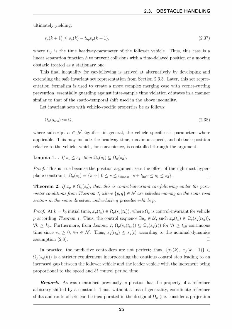
Figure 2.11: Car-following with xp ∈ Ωp(sq).
function with the expression xp ∈ Ωp(sq) where sq = sq +L has been shifted by a constantL). This is a practical way to account for vehicle length as well as additional safety zonesby reducing the available gap.
From the invariant set, the follower vehicle is granted the choice of a feasible stop-ping trajectory that makes no assumptions based on the leader vehicle’s dynamics (seeFigure 2.11). On the contrary, the Time-To-Collision (TTC) approaches allow close gapsof mere meters in platooning scenarios, even at high speeds, enabling vehicles to takeadvantage of reduced air drag and more closely packed traffic for greater road utilisation.However, these approaches are built on a solid knowledge of various factors, includingdynamics and vehicle control, procedures for joining and leaving a platoon and trus-ted low-latency communication. In platoons, vehicle sequences are designed to providesafe, collision-free trajectories, even during emergency braking; they exploit the levelof similarity and slight differences between vehicle capabilities through synchronised ac-tions. It is easy to see how homogeneous platoon of vehicles simultaneously executingidentical actions would result in the maintenance of any positive gaps, providing infiniteTTC and safety. In realistic scenarios; however, any invalid assumption could result in acollision—even a simple deceleration would yield non-intuitive trajectory variations dueto unmodelled and higher order terms (e.g. disc brake characteristics due to hydraulic ac-tuation and delays, built-in pedal and calliper mechanisms, and tribological factors suchas brake surface wear and fading). Ascertaining the appropriate separation between suchtrajectories is computationally difficult and would require comprehensive and continuousknowledge of such trajectories in real time, or even ahead of time.
26
2.3. OBSTACLE HANDLING
2.3.5 Safe merging
A proposed framework for safe-merging builds on the static-obstacle approach and car-following modes. Consider the following aggregated set:
Ωpq := xp, xq|xp ∈ Ωp(L1) ∨xq ∈ Ωq(L2) ∨xp ∈ Ωp(sq+L3) ∨xq ∈ Ωq(sp−L4), (2.39)
where the two–two modes relate to the original obstacle Cpq and its four sides, as shownin Figure 2.4.
From Theorem 1 and Theorem 2, it is safe to conclude that:
[xk0p , xk0q ] ∈ Ωpq =⇒ ∃up ∈ (up, uq) ∈ (Up,Uq), [xkp, x
kq ] ∈ Ωpq, k ≥ k0,
which satisfies the[xkp, x
kq
]/∈ Cpq condition.
However, this may be violated within the t ∈ (tk, tk+1) continuous time interval, res-ulting in collisions:
∀[xkp, xkq ], [xk+1p , xk+1
q ] ∈ Ωpq, ; [xp(t), xq(t)] /∈ Cpq, t ∈ (tk, tk+1).
An obvious case of this phenomenon is when a leader vehicle and a follower vehicleswitch roles between two discrete time steps; this is referred to as corner-cutting, a char-acteristic issue of discrete-time constrained problems and non-convex obstacle avoidance.
2.3.5.1 Corner-cutting prevention
The disadvantageous cut of the solution trajectory into the obstacle region (i.e. vehiclecollision) in continuous time may happen in cases were trajectories are constrained onlyat discrete time steps, mainly around constraints defining obstacle corners [63]. Thisphenomenon can be avoided through corner-cutting prevention—also known as inter-sample avoidance—by requiring a handover between discrete time steps and modes. Theenforcement of a temporal handover between discrete time steps is often implemented inMIP formulation either through logical constraints between binaries [50] or by duplicatingand temporally shifting the modes (active set of constraints) [70].
Let the safety-preserving modes from (2.39) be named as:
m1 : xp ∈ Ωp(L1),
m2 : xq ∈ Ωq(L2),
m3 : xp ∈ Ωp(sq + L3),
m4 : xq ∈ Ωq(sp + L4).
(2.40)
Each mode has an alternative interpretation of a positive control-invariant safe set ofstates. A state is able to remain in any mode set safely and indefinitely if it is already
27
CHAPTER 2. VEHICULAR CONTROL WITH TIME-HEADWAY MI-MPC
part of that set and chooses to remain as such (see positive control invariance).Now let the following sequence show with (T: true; −: false) when different modes are
active and set constraints are satisfied:
k − 3 k − 2 k − 1 k k + 1 k + 2 k + 3
m1 T T T T − − −m2 T T − − − − −m3 − − − T T T T
m4 − − − − − − −
The states must be safe at any k discrete time; thus, at least one mode must be activeat each time for all pairwise vehicle-interaction obstacles. This consideration relates tothe separating hyperplane theorem [60].
Furthermore, both modes have to be active (true) at the moment of handover forcorner-cutting prevention between switching modes, as shown in the above example at k.
Suppose the new set Ωccppq := Ωpq(+binary logic) is designed to be control-invariant
and collision-free with respect to continuous time. This can be achieved by implementingthe logic of two methods from [50, 70], which are compared in [63] using the big-Mapproach. The advantage of using the approach in [70] with duplicated and temporallyshifted original constraints stems from the improved scaling and less sensitive numericsin binary logic. As such, it is the preferred implementation later in this work.
For example, the transition m1 → m3 at k represents the entrance into car-followingmode; aforementioned logic of corner-cutting prevention would yield a smaller set of states:
xp(k) ∈ Ωp(L1) ∩ Ωp(sq + L3),
which can cause additional artefacts when the state evolution is large between the timestep, especially for long periods times. Mitigation for these artefacts using shadow-regiondescription is considered to be a less strict formulation [56, p. 65], in which hyperplanesseparating the next state are generated as a function of the linear visibility from theprevious state. However, this would remove the convex structure of the problem whenthe binaries are fixed.
2.4 Feasible paths to goal
This section discusses the possibility and practicality of feasible and non-feasible pathsto reach vehicle goals in the face of obstacle shapes, positions and, in cases of multipleobstacles, their constellations. The obstacles from the junction interaction collision setsare convex; however, the exclusion of such sets generally makes their optimisation non-convex, imposing the risk of local minima or unattainable goal positions. Furthermore,
28
2.4. FEASIBLE PATHS TO GOAL
on account of the finite-length planning horizons, an earlier decision of vehicle orders maylater impede the progress of vehicles toward their goals and trap the solution trajectory.For examples, in Figure 2.12 (a), (c) and (e), see how the B paths around the obstaclesend up trapped and fail to reach the goal position for one or both vehicles (withoutreversing). These situations represent cases in which both the vehicle goal position andthe vehicle interaction (collision set) act as an obstacle. Thus, a constellation of multipleobstacles, even if the individual elements are convex, is inherently able to form traps.
In Figure 2.12 (b), (d) and (f), in contrast, either vehicle order gives way to a solutionto reach the vehicle goals—no obstacles overlap. In this work, the examples address casesin which the vehicle order has a neutral effect on goal reachability. In most cases, goalreachability issues are not present in simple junction simulations, as vehicles never intendto park in the vicinity of the junction; rather, they aim to leave the area of junction (i.e.the goals are far, usually outside of the simulated area).
However, when multiple vehicles interact, the multiple collision sets may form non-convex obstacles with traps in higher-dimensional state space from the amalgam of convexpair-wise collision sets (represented in the higher dimensional state space). Following thereasoning in [57], the global solution is attainable when the system has a sequence ofvehicles represented on a priority graph without loops [30]. The intuitive way to showthat junction simulations without cyclic priority graphs are able to reach their solutionis phrased in [57]. Namely, if the system (junction simulation) always has at least onevehicle that can freely move forward and either reach its non-obstructing goal or leave thesystem, the system eventually clears up and all vehicles can eventually reach their goalor leave the system.
Remark: Here the above idea in [57] is rephrased. If a feasible path is transferring thevehicles to their goal position with non-changing system parameters and obstacles, then∀tk,∃n ∈ N , such that vehicle n had a free choice to move, vn(tk) > 0, when sn(tk) < sn G.
In practice, positive vehicle speeds can be indicators of progress and liveliness thoughasymptotic speed profiles for deceleration in a trap would satisfy this condition.
The convexity of the obstacles, even in a single pair-wise collision set case, is notsatisfying as obstacle avoidance from certain state configurations can only be done throughreversal, which is against the non-negative speed constraint. For example, imagine amerging or box obstacle (Figure 2.12) with, in place of the bottom-left right angle, anobtuse one; the shape would still be convex but the feature would act as a trap withoutthe ability to reverse. Thus, all collision sets are required to be convex (satisfied by thesupporting hyperplane description) and have all obstacle boundaries in any point allowat least one vehicle to have positive speed towards its goal:
max
(∂gi(sp, sq, vp)
∂sp,∂gi(sp, sq, vp)
∂sq
)> 0, ∀i = 1 . . . Npq,h, (2.41)
29
CHAPTER 2. VEHICULAR CONTROL WITH TIME-HEADWAY MI-MPC
where the i-th hyperplane is gi ≤ 0, and the number of hyperplanes that define thecollision set (obstacle) is Npq,h.
Remark: this condition is true for single or separate obstacle cases; as mentioned,multiple convex obstacles are still able to form a non-convex union obstacle when overlaid.For example, this can happen when vehicles are trapped in a gridlock prone intersection,reaching a local minimum of the problem; the obstacle in such a case forms a pocket inthe higher-dimensional configuration space and traps the system state once it has enteredinto the pocket. Intuitively, in the higher-dimensional space, it is necessary for at leastone of the vehicles to be able to move at any obstacle-free point in the configurationspace; it is generally possible to formulate a condition similar to (2.41). In this work, onlyatomic junction blocks are examined, as they are simple enough to be not prone for suchstructural gridlocks.
Let the combined obstacle set be defined by the union set of collision positions, whereeach 2D collision set is extruded to the high-dimensional space of the total number ofagents. First, by redefining Cpq, it would cast itself to the appropriate dimensional spaceof RN , N > 2:
Cpq =s ∈ RN | [sp, vp, sq, vq] ∈ Cpq, vp = vq = 0
(2.42)
This extrudes the pairwise collision sets into the higher dimension. Following this, let theoverall obstacle be the union of all pairwise collision sets:
C =⋃
∀p∈N ,q∈N ,p 6=q
Cpq (2.43)
then requiring
sk, sG /∈ C (2.44)
with the previous requirement on hyperplanes, (2.41), it is ensured that a trajectoryexists between current sk and goal position sG. The completion time of this trajectorymay, however, depend on vehicle-specific dynamics. Consider the worst-case scenario:the trajectory exists only when the previously moving vehicle p has zero speed. While inmotion, the safety constraints allow for a full stop; however, if asymptotic convergenceis assumed, the convergence time may be ∞. This would mean that, in some situations,the vehicles are so tightly packed that they temporarily block one another, which, in apractical sense, is still solvable. The model considers a certain safety length over thephysical vehicle length. When slow convergence occurs, it may be beneficial to give upa portion of the safety distance at low speeds to allow for reasonable vehicle progress.Alternatively, a better suited controller could be switched to and optimise trajectory withhigh-fidelity models for close vehicle manoeuvres (complete motion planning). It may
30
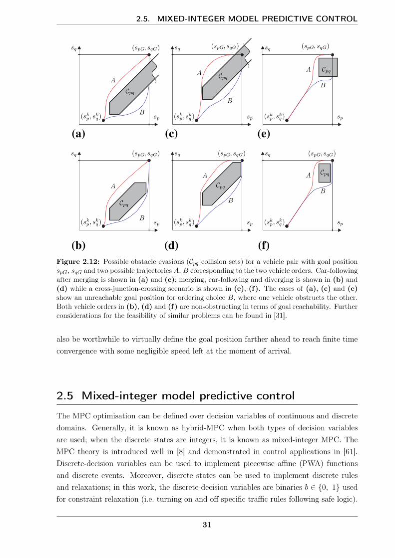
2.5. MIXED-INTEGER MODEL PREDICTIVE CONTROL
Figure 2.12: Possible obstacle evasions (Cpq collision sets) for a vehicle pair with goal positionspG, sqG and two possible trajectories A, B corresponding to the two vehicle orders. Car-followingafter merging is shown in (a) and (c); merging, car-following and diverging is shown in (b) and(d) while a cross-junction-crossing scenario is shown in (e), (f). The cases of (a), (c) and (e)show an unreachable goal position for ordering choice B, where one vehicle obstructs the other.Both vehicle orders in (b), (d) and (f) are non-obstructing in terms of goal reachability. Furtherconsiderations for the feasibility of similar problems can be found in [31].
also be worthwhile to virtually define the goal position farther ahead to reach finite timeconvergence with some negligible speed left at the moment of arrival.
2.5 Mixed-integer model predictive control
The MPC optimisation can be defined over decision variables of continuous and discretedomains. Generally, it is known as hybrid-MPC when both types of decision variablesare used; when the discrete states are integers, it is known as mixed-integer MPC. TheMPC theory is introduced well in [8] and demonstrated in control applications in [61].Discrete-decision variables can be used to implement piecewise affine (PWA) functionsand discrete events. Moreover, discrete states can be used to implement discrete rulesand relaxations; in this work, the discrete-decision variables are binaries b ∈ 0, 1 usedfor constraint relaxation (i.e. turning on and off specific traffic rules following safe logic).
31

CHAPTER 2. VEHICULAR CONTROL WITH TIME-HEADWAY MI-MPC
The MPC problem with a horizon length of Np and multiple agents results in thefollowing optimisation problem:MPC-2.3
J∗MPC-2.3 = min∑n∈N
Np−1∑j=0
ln (xn (k + j + 1|k) , un (k + j|k))
s.t. ∀j ∈ 0 . . . (Np − 1), ∀n ∈ N :
xn (k|k) = xn (k)
xn (k + j + 1|k) = A xn (k + 1|k) +B un (k + 1|k)
xn ∈ Xnun ∈ Un
and ∀p, q ∈ N , p 6= q, Cpq 6= ∅ :
[xp, xq] ∈ Ωccppq ,
where the operational constraints for the states are encoded in Xn (e.g. speed range) andfor control inputs Un (e.g. acceleration range). The cost function is chosen to be a simplequadratic ‘running-cost’, which is discussed in depth later in the work. The stage costsin the cost formulation are as follows:
ln (xn, un) = Q (vn − vd n)2 +R u2n, (2.46)
where the quadratic cost weights are Q and R and the agent-wise desired speed is vd n.The logic is contained in Ωccp
pq , which selects the necessary constraints to realise the control-invariant sets. The logic is based on binary decision variables, a sub-class of integers ren-dering the overall problem as a mixed-integer program (MIP). The original, non-negativespeed assumption reappears in Ωccp
pq definitions and is already included in the domainXn of states. Without duplicating the two speed limits, only the hyperplane separatingx states and the separating hyperplane theorem constraint needs to be added. Let thisconstraint for the modes in general for vehicle n ∈ p, q be represented as:
g(xn, sobs; thn) ≤ 0.
The big-M relaxation method was chosen to relax the linear inequality constraints becauseit is a straightforward formulation, does not add additional non-convexities to the problem,and does not increase the problem size [38]. Through this relaxation, a constraint ispractically activated or deactivated as:
g(xn, sobs; thn) ≤M b,
32

2.5. MIXED-INTEGER MODEL PREDICTIVE CONTROL
where a sufficiently large constant is M and a binary decision variable is b ∈ 0, 1. Infact, according to [8], M is to be chosen as:
M , maxx∈X
g(x, sobs; thn). (2.47)
In practice, only some of the examples shown have fully bounded X domains, for whichM can be chosen to respect the boundaries. If this is not possible, M is chosen to benon-restrictive in the simulations, given the practical sizes of the numerical test region aswell as the distance covered over the horizon lengths. The tightness of the constraints inthe big-M formulation strongly depends on the size of M ; consequently, a smaller M isbetter, though the formulation is still weak by nature when compared to other relaxationmethods [38].
Moreover, the formulation used is not well-posed, according to [8], because the b binarystates are not unique indicators of the violation state of the relaxed inequality (i.e. whenb ≡ 1, the respected inequality may be either satisfied or in a violated state). This doesnot compromise the relaxation formulation; however, it may impose a performance trade-off between well-posed binaries with extra overhead and better branch-and-bound searchspeeds.
In practice, the four modes can be simplified as four linear inequalities (hyperplanes)and the connecting logic:
g1(xp, L1; thp) ≤M b1 (2.48a)
g2(xq, L2; thq) ≤M b2 (2.48b)
g3(xp, sq + L3; thp) ≤M b3 (2.48c)
g4(xq, sp + L4; thq) ≤M b4 (2.48d)4∑
m=1
bm ≤ 3. (2.48e)
Note that when bm ≡ 1, the corresponding inequality is relaxed. Moreover, (2.48e) in-equality ensures that at least one of the four modes is active (not relaxed), which repres-ents the logic of the separating hyperplane theorem. Thus, the above set of inequalities in(2.48a)-(2.48e), and (2.9) encode Ωpq. Recall that corner-cutting between two time-steps kand k+1 can still happen when the subsequent states [xkp, x
kq ] ∈ Ωpq and [xk+1
p , xk+1q ] ∈ Ωpq.
Thus, following the method [63, 70] as discussed in Section 2.3.5.1 the corner-cutting pre-
33

CHAPTER 2. VEHICULAR CONTROL WITH TIME-HEADWAY MI-MPC
vention employs binaries and yields:
g1(xp(k), L1; thp) ≤M b1(k) (2.49a)
g2(xq(k), L2; thq) ≤M b2(k) (2.49b)
g3(xp(k), sq(k) + L3; thp) ≤M b3(k) (2.49c)
g4(xq(k), sp(k) + L4; thq) ≤M b4(k) (2.49d)4∑
m=1
bm(k) ≤ 3 (2.49e)
g1(xp(k + 1), L1; thp) ≤M b1(k) (2.49f)
g2(xq(k + 1), L2; thq) ≤M b2(k) (2.49g)
g3(xp(k + 1), sq(k + 1) + L3; thp) ≤M b3(k) (2.49h)
g4(xq(k + 1), sp(k + 1) + L4; thq) ≤M b4(k), (2.49i)
where the same binaries are enforced for the next time step for the mode constraints. Thissatisfies the logic between the time steps outlined in the requirements of Ωccp
pq , providingthe safe transition between modes and naturally increasing the number of inequalitiesfrom five to nine.
2.5.1 Robustness for sudden stop events
The further extension of spatio-temporal constraints provides a stricter formulation andadds robustness against sudden stop events that may occur during low-speed urban drivingor as a result of general mismatch between predicted and actual states. Suppose thatobstacle position sq(k+ 1) in (2.49h) is replaced with sq(k). When this change is appliedto both (2.49h) and (2.49i), it results in:
g3(xp(k + 1), sq(k) + L3, thp) ≤M b3(k) (2.50)
g4(xq(k + 1), sp(k) + L4, thq) ≤M b4(k), (2.51)
where the new position of the follower vehicle must respect the obstacle position that isdetermined by the current position of the leader without making any assumptions aboutthe vehicle dynamics of the leader.
In this case, observe that from the four modes for m1 and m3, xkp ∈ Ωp(sobs(k)) andxk+1p ∈ Ωp(sobs(k)). This means that vehicle p is not only capable of controlling its future
states to remain in the control-invariant set but is also required to remain in that setfor the next time step. For example, this formula decouples the time-dependent termsof the leader vehicle dynamics, treating it like a true static obstacle between time steps,which results in a more conservative but safe set against sudden stops referred to by the
34

2.6. NUMERICAL TESTS: MERGING WITH TWO VEHICLES
combined Ωccp,stpq :
Ωccp,stpq (k) := xkp, xk+1
p , xkq , xk+1q , bki , i = 1, . . . 4|(2.49a)–(2.49g), (2.50), (2.51) (2.52)
Remark: Suppose the system is represented by only (2.49e)–(2.49g), (2.50) and (2.51).This would, for example, simplify in m1 and m3 modes to xk+1
p ∈ Ωp(sobs(k)) constraintset (with only the states of the next time step xk+1
p , allowing for a larger attractor set forxkp initial states), increasing the noise tolerance and recovery capabilities of the controlwithout explicitly needing to calculate such an attractor set. However, the corner-cuttingprevention logic expects constraint feasibility checks for both discrete times and requiresxkp, x
k+1p states, which is easier to be fulfilled by the full Ωccp,st
pq (k) set.
2.6 Numerical tests: Merging with two vehicles
Feasibility tests for Y-junction merging were conducted with two identical vehicles fordifferent th–δt parameter pairs. Initial speeds were set to v0 = vmax = vdes = 10 ms−1.Initial positions were chosen randomly to provide conflicting arrivals at the junction; thechosen positions were far enough from the junction to respect initial feasibility and non-interfering predictions (i.e. s0p ≤ L1
pq − (thp + Npδt)v0 ). The following parameters were
chosen: time horizon Np = 5, amin = −9.81/2 ms−2 and amax = 3 ms−2; for simplicity,soff1 = soff2 = 0 m; L1 = L2 = 4 m.MPC-2.4
J∗MPC2.4 = min∑n∈N
Np−1∑j=0
ln (xn (k + j + 1|k) , un (k + j|k)) (2.53a)
s.t. ∀j ∈ 0 . . . (Np − 1), ∀n ∈ N :
xn (k|k) = xn (k)
xn (k + j + 1|k) = A xn (k + 1|k) +B un (k + 1|k)
xn ∈ Xnun ∈ Un
and ∀p, q ∈ N , p 6= q, Cpq 6= ∅ :
[xp, xq] ∈ Ωccp,stpq .
The cost function to be minimised is set to quadratic speed error penalisation withoutacceleration penalty terms (R = 0), as this allows for better state mapping due to the
35
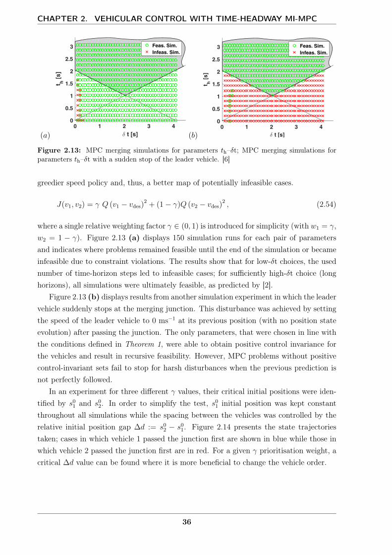
CHAPTER 2. VEHICULAR CONTROL WITH TIME-HEADWAY MI-MPC
(a) (b)
Figure 2.13: MPC merging simulations for parameters th–δt; MPC merging simulations forparameters th–δt with a sudden stop of the leader vehicle. [6]
greedier speed policy and, thus, a better map of potentially infeasible cases.
J(v1, v2) = γ Q (v1 − vdes)2 + (1− γ)Q (v2 − vdes)2 , (2.54)
where a single relative weighting factor γ ∈ (0, 1) is introduced for simplicity (with w1 = γ,w2 = 1 − γ). Figure 2.13 (a) displays 150 simulation runs for each pair of parametersand indicates where problems remained feasible until the end of the simulation or becameinfeasible due to constraint violations. The results show that for low-δt choices, the usednumber of time-horizon steps led to infeasible cases; for sufficiently high-δt choice (longhorizons), all simulations were ultimately feasible, as predicted by [2].
Figure 2.13 (b) displays results from another simulation experiment in which the leadervehicle suddenly stops at the merging junction. This disturbance was achieved by settingthe speed of the leader vehicle to 0 ms−1 at its previous position (with no position stateevolution) after passing the junction. The only parameters, that were chosen in line withthe conditions defined in Theorem 1, were able to obtain positive control invariance forthe vehicles and result in recursive feasibility. However, MPC problems without positivecontrol-invariant sets fail to stop for harsh disturbances when the previous prediction isnot perfectly followed.
In an experiment for three different γ values, their critical initial positions were iden-tified by s01 and s02. In order to simplify the test, s01 initial position was kept constantthroughout all simulations while the spacing between the vehicles was controlled by therelative initial position gap ∆d := s02 − s01. Figure 2.14 presents the state trajectoriestaken; cases in which vehicle 1 passed the junction first are shown in blue while those inwhich vehicle 2 passed the junction first are in red. For a given γ prioritisation weight, acritical ∆d value can be found where it is more beneficial to change the vehicle order.
36
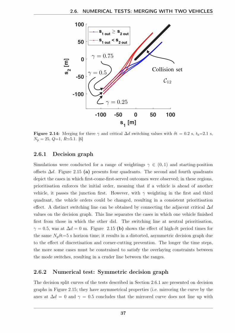
2.6. NUMERICAL TESTS: MERGING WITH TWO VEHICLES
Figure 2.14: Merging for three γ and critical ∆d switching values with δt = 0.2 s, th=2.1 s,Np = 25, Q=1, R'5.1. [6]
2.6.1 Decision graph
Simulations were conducted for a range of weightings γ ∈ (0, 1) and starting-positionoffsets ∆d. Figure 2.15 (a) presents four quadrants. The second and fourth quadrantsdepict the cases in which first-come-first-served outcomes were observed; in these regions,prioritisation enforces the initial order, meaning that if a vehicle is ahead of anothervehicle, it passes the junction first. However, with γ weighting in the first and thirdquadrant, the vehicle orders could be changed, resulting in a consistent prioritisationeffect. A distinct switching line can be obtained by connecting the adjacent critical ∆d
values on the decision graph. This line separates the cases in which one vehicle finishedfirst from those in which the other did. The switching line at neutral prioritisation,γ = 0.5, was at ∆d = 0 m. Figure 2.15 (b) shows the effect of high-δt period times forthe same Npδt=5 s horizon time; it results in a distorted, asymmetric decision graph dueto the effect of discretisation and corner-cutting prevention. The longer the time steps,the more some cases must be constrained to satisfy the overlaying constraints betweenthe mode switches, resulting in a cruder line between the ranges.
2.6.2 Numerical test: Symmetric decision graph
The decision split curves of the tests described in Section 2.6.1 are presented on decisiongraphs in Figure 2.15; they have asymmetrical properties (i.e. mirroring the curve by theaxes at ∆d = 0 and γ = 0.5 concludes that the mirrored curve does not line up with
37
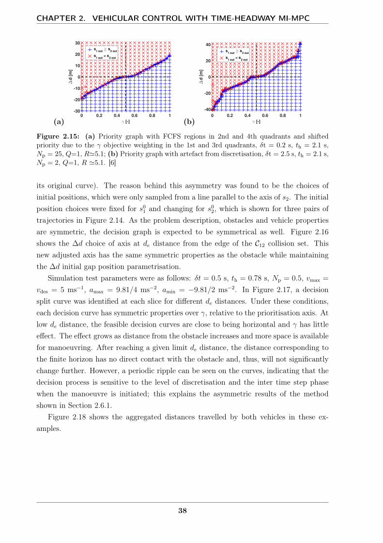
CHAPTER 2. VEHICULAR CONTROL WITH TIME-HEADWAY MI-MPC
(a)0 0.2 0.4 0.6 0.8 1
γ [-]
-30
-20
-10
0
10
20
30
∆d
[m
]
s1 out
≥ s2 out
s1 out
< s2 out
(b)0 0.2 0.4 0.6 0.8 1
γ [-]
-40
-20
0
20
40
∆d
[m
]
s1 out
≥ s2 out
s1 out
< s2 out
Figure 2.15: (a) Priority graph with FCFS regions in 2nd and 4th quadrants and shiftedpriority due to the γ objective weighting in the 1st and 3rd quadrants, δt = 0.2 s, th = 2.1 s,Np = 25, Q=1, R'5.1; (b) Priority graph with artefact from discretisation, δt = 2.5 s, th = 2.1 s,Np = 2, Q=1, R '5.1. [6]
its original curve). The reason behind this asymmetry was found to be the choices ofinitial positions, which were only sampled from a line parallel to the axis of s2. The initialposition choices were fixed for s01 and changing for s02, which is shown for three pairs oftrajectories in Figure 2.14. As the problem description, obstacles and vehicle propertiesare symmetric, the decision graph is expected to be symmetrical as well. Figure 2.16shows the ∆d choice of axis at de distance from the edge of the C12 collision set. Thisnew adjusted axis has the same symmetric properties as the obstacle while maintainingthe ∆d initial gap position parametrisation.
Simulation test parameters were as follows: δt = 0.5 s, th = 0.78 s, Np = 0.5, vmax =
vdes = 5 ms−1, amax = 9.81/4 ms−2, amin = −9.81/2 ms−2. In Figure 2.17, a decisionsplit curve was identified at each slice for different de distances. Under these conditions,each decision curve has symmetric properties over γ, relative to the prioritisation axis. Atlow de distance, the feasible decision curves are close to being horizontal and γ has littleeffect. The effect grows as distance from the obstacle increases and more space is availablefor manoeuvring. After reaching a given limit de distance, the distance corresponding tothe finite horizon has no direct contact with the obstacle and, thus, will not significantlychange further. However, a periodic ripple can be seen on the curves, indicating that thedecision process is sensitive to the level of discretisation and the inter time step phasewhen the manoeuvre is initiated; this explains the asymmetric results of the methodshown in Section 2.6.1.
Figure 2.18 shows the aggregated distances travelled by both vehicles in these ex-amples.
38
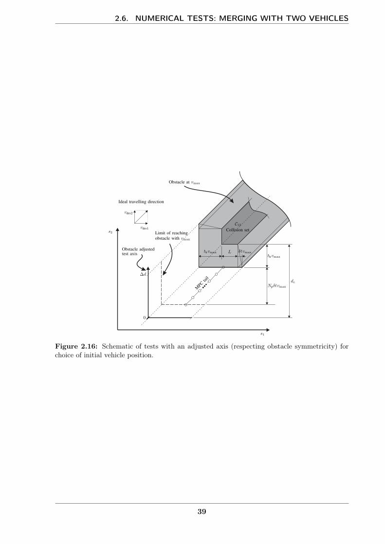
2.6. NUMERICAL TESTS: MERGING WITH TWO VEHICLES
Figure 2.16: Schematic of tests with an adjusted axis (respecting obstacle symmetricity) forchoice of initial vehicle position.
39

CHAPTER 2. VEHICULAR CONTROL WITH TIME-HEADWAY MI-MPC
(a)
-10
0
-5
0
5
d
5
1
de
10
10
0.80.615
0.40.2
20 0
(b)0 0.2 0.4 0.6 0.8 1
-15
-10
-5
0
5
10
15
d
Figure 2.17: In (a), the feasible-decision critical ∆d curves are shown for different de distancesfrom the obstacle and γ prioritisations. (b) shows the side view of (a). The further the initialvehicle positions (starting with vmax) are from the obstacle, the more significant the influenceof relative prioritisation γ is over ∆d while the curves remain symmetric; after a given limitdistance, the curves display periodicity.
40
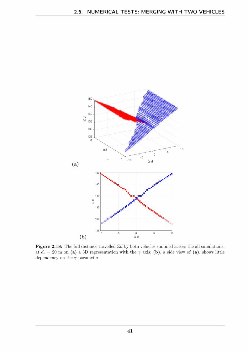
2.6. NUMERICAL TESTS: MERGING WITH TWO VEHICLES
(a)
125
0
130
135
140
d
145
100.5
150
5
d
0-5
1 -10
(b)-10 -5 0 5 10
d
125
130
135
140
145
150
d
Figure 2.18: The full distance travelled Σd by both vehicles summed across the all simulations,at de = 20 m on (a) a 3D representation with the γ axis; (b), a side view of (a), shows littledependency on the γ parameter.
41

CHAPTER 2. VEHICULAR CONTROL WITH TIME-HEADWAY MI-MPC
2.7 Numerical tests: Four lanes and vehicles merging
This section presents numerical tests of a scenario in which four vehicles merge from fourdifferent lanes (see Figure 2.19).
Vehicular control for four-lane merging is detailed in MPC 2.5, where the merginginteractions are collected in NMI with vehicle pair tuples p, q ∈ NMI. The numberof tuples in NMI is NMI, which is ‘four choose two’ for this case, NMI = 6 because twoelement subsets (vehicle pairs) are chosen from the four-element vehicle set N . Theparameters in the example were chosen as follows: δt=1 s, th=2.1 s, Np = 5, the vehicleweights are wn=1...4=[0.25, 0.05, 0.1, 0.6] for n = 1 . . . 4 vehicle indices, Q=1, R'5.1 andsoffn=1...4=0 with vehicle length L = 4 m, making the obstacle geometries identical withL1 = L2 = L3 = L4 = −L. The desired speed is vd = 9 ms−1 while the maximum speed isvmax = 10 ms−1. The position evolution of the four vehicles is shown in Figure 2.20; theirspeeds are shown in Figure 2.21. It is verified by the simulated trajectories, that by settingrelative priorities for the vehicles (ωn), they act in a cooperative manner. In the example,high priority vehicles merge first at the junction before accelerating or decelerating backto their desired speed. In Figure 2.21, the first vehicle to merge is shown to increase itsspeed over its desired speed in order to ease the control actions of the vehicles behind it.
Figure 2.19: Four separate lanes merging to one lane
42

2.7. NUMERICAL TESTS: FOUR LANES AND VEHICLES MERGING
MPC-2.5
J∗MPC-2.5 = min∑n∈N
Np−1∑j=0
ωn ln (xn (k + j + 1|k) , un (k + j|k)) (2.55a)
s.t. ∀j ∈ 0 . . . (Np − 1), ∀n ∈ N :
xn (k|k) = xn (k)
xn (k + j + 1|k) = A xn (k + j|k) +B un (k + j|k)
xn ∈ Xnun ∈ Un
and ∀p, q ∈ NMI :
sp(k + j|k) + thvp(k + j|k) ≤ L1 +M bpq 1(k + j|k)
sq(k + j|k) + thvq(k + j|k) ≤ L2 +M bpq 2(k + j|k)
sp(k + j|k) + thvp(k + j|k) ≤ sq(k + j|k) + L3 +M bpq 3(k + j|k)
sq(k + j|k) + thvq(k + j|k) ≤ sp(k + j|k) + L4 +M bpq 4(k + j|k)
4∑m=1
bpq m(k + j|k) ≤ 3
sp(k + j + 1|k) + thvp(k + j + 1|k) ≤ L1 +M bpq 1(k + j|k)
sq(k + j + 1|k) + thvq(k + j + 1|k) ≤ L2 +M bpq 2(k + j|k)
sp(k + j + 1|k) + thvp(k + j + 1|k) ≤ sq(k + j|k) + L3 +M bpq 3(k + j|k)
sq(k + j + 1|k) + thvq(k + j + 1|k) ≤ sp(k + j|k) + L4 +M bpq 4(k + j|k).
43
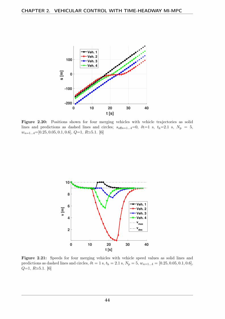
CHAPTER 2. VEHICULAR CONTROL WITH TIME-HEADWAY MI-MPC
0 10 20 30 40
t [s]
-200
-100
0
100s [
m]
Veh. 1
Veh. 2
Veh. 3
Veh. 4
Figure 2.20: Positions shown for four merging vehicles with vehicle trajectories as solidlines and predictions as dashed lines and circles; soffn=1...4=0, δt=1 s, th=2.1 s, Np = 5,wn=1...4=[0.25, 0.05, 0.1, 0.6], Q=1, R'5.1. [6]
0 10 20 30 40
t [s]
2
4
6
8
10
v [
m]
Veh. 1
Veh. 2
Veh. 3
Veh. 4
vmax
vdes
Figure 2.21: Speeds for four merging vehicles with vehicle speed values as solid lines andpredictions as dashed lines and circles, δt = 1 s, th = 2.1 s, Np = 5, wn=1...4 = [0.25, 0.05, 0.1, 0.6],Q=1, R'5.1. [6]
44
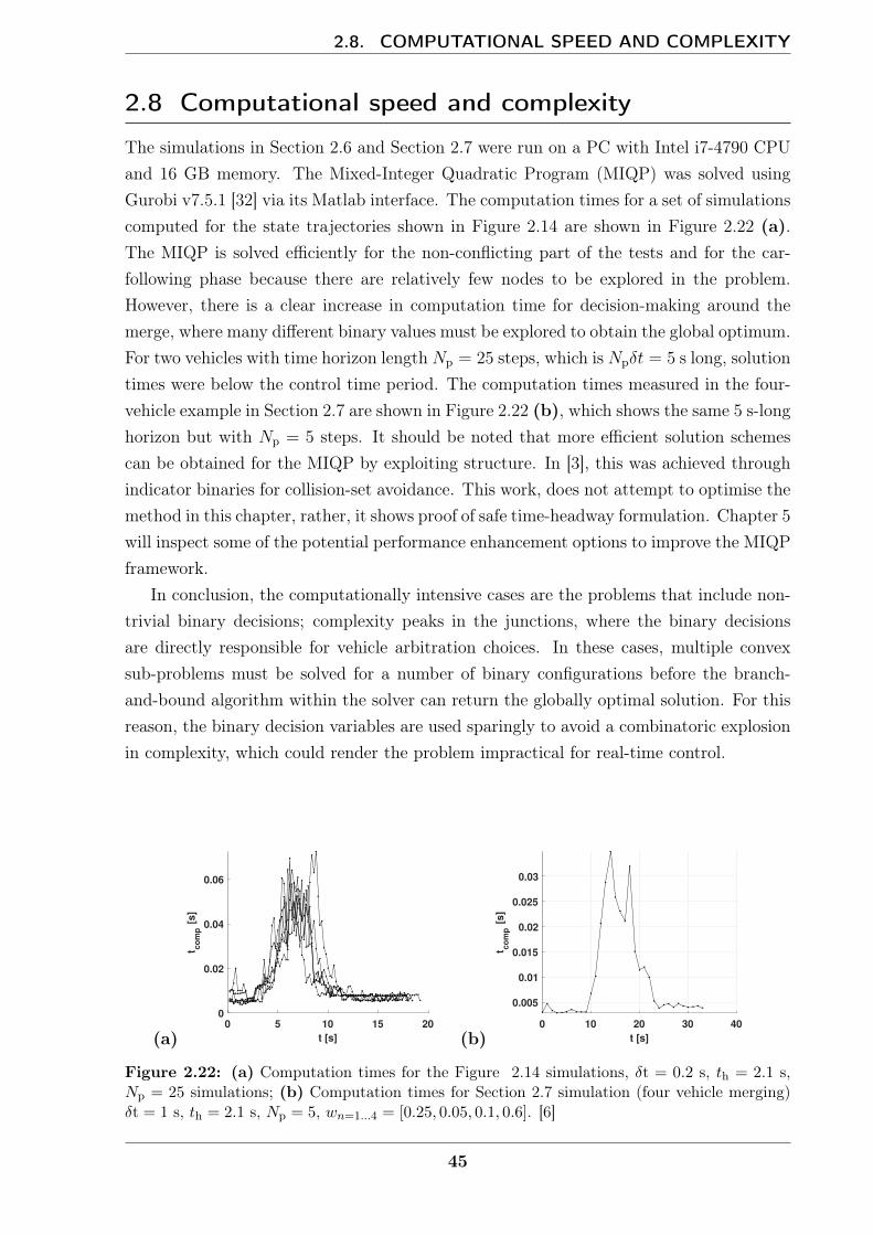
2.8. COMPUTATIONAL SPEED AND COMPLEXITY
2.8 Computational speed and complexity
The simulations in Section 2.6 and Section 2.7 were run on a PC with Intel i7-4790 CPUand 16 GB memory. The Mixed-Integer Quadratic Program (MIQP) was solved usingGurobi v7.5.1 [32] via its Matlab interface. The computation times for a set of simulationscomputed for the state trajectories shown in Figure 2.14 are shown in Figure 2.22 (a).The MIQP is solved efficiently for the non-conflicting part of the tests and for the car-following phase because there are relatively few nodes to be explored in the problem.However, there is a clear increase in computation time for decision-making around themerge, where many different binary values must be explored to obtain the global optimum.For two vehicles with time horizon length Np = 25 steps, which is Npδt = 5 s long, solutiontimes were below the control time period. The computation times measured in the four-vehicle example in Section 2.7 are shown in Figure 2.22 (b), which shows the same 5 s-longhorizon but with Np = 5 steps. It should be noted that more efficient solution schemescan be obtained for the MIQP by exploiting structure. In [3], this was achieved throughindicator binaries for collision-set avoidance. This work, does not attempt to optimise themethod in this chapter, rather, it shows proof of safe time-headway formulation. Chapter 5will inspect some of the potential performance enhancement options to improve the MIQPframework.
In conclusion, the computationally intensive cases are the problems that include non-trivial binary decisions; complexity peaks in the junctions, where the binary decisionsare directly responsible for vehicle arbitration choices. In these cases, multiple convexsub-problems must be solved for a number of binary configurations before the branch-and-bound algorithm within the solver can return the globally optimal solution. For thisreason, the binary decision variables are used sparingly to avoid a combinatoric explosionin complexity, which could render the problem impractical for real-time control.
(a)0 5 10 15 20
t [s]
0
0.02
0.04
0.06
t co
mp
[s]
(b)0 10 20 30 40
t [s]
0.005
0.01
0.015
0.02
0.025
0.03
t co
mp
[s
]
Figure 2.22: (a) Computation times for the Figure 2.14 simulations, δt = 0.2 s, th = 2.1 s,Np = 25 simulations; (b) Computation times for Section 2.7 simulation (four vehicle merging)δt = 1 s, th = 2.1 s, Np = 5, wn=1...4 = [0.25, 0.05, 0.1, 0.6]. [6]
45

46
3Cost and predictions
This chapter starts with a brief general overview of the cost function choices. Later inthis chapter, the basic structure and elements of the cost functions used in this workare introduced in order to compare two formulations. The ‘running-cost’ formulation iswidely used in the literature on vehicle control, but has unreachable speed reference whenthe vehicle is close to an obstacle or needs to stop, which is an operational mode for safety(see Chapter 2). This makes it difficult to obtain stability results; thus, stability resultsare acquired through a different cost formulation, with an objective corresponding to asoft form of the safety constraint. With proper parameter tuning (i.e. exact penalty), thesame behaviours are observed with both cost formulations.
3.1 Overview
The velocity optimisation introduced in Chapter 2 uses binary variables to relax hyper-plane constraints from obstacle avoidance in the hybrid-MPC formulation. Accordingto Theorem 1, simple time-headway parameters provide positive-control-invariant sets tooperate in and yield safe/recursively feasible operations. This chapter focuses on otheraspects of the controller, namely the cost function that aims to encapsulate the goals andobjectives in the optimised performance metric, while providing some stability results.For a more extensive introduction to the basics of cost functions, see [11, 59].
The approaches proposed in this work aim to obtain the globally optimal solutionsubject to obstacle avoidance. Obstacle avoidance is inherently an NP-hard problem andin this work formulated into an NP-complete problem with the use of binary relaxations.This enables commercially available branch-and-bound solvers to obtain the globally op-timal solution, where, for each fixed binary configuration, the problem reverts itself to aconvex QP optimisation.
It may be argued that formulating the problem to be a global method (to obtainglobally optimal results) is very restrictive. For this reason, it may be better to solve
47

CHAPTER 3. COST AND PREDICTIONS
a less idealised formulation to sub-optimality with local solvers than to get the globallyoptimal solution to a cruder problem.
It should be noted that when problem convexity is less of a concern, more optionsare available for the problem formulations. These include non-convex cost functions (e.g.general utility functions) [83], non-linear system dynamics (e.g. steering in 2D problems)[67] and non-convex constraints in general (e.g. non-convex vehicle shapes and obstacles)[68].
Economic MPC is concerned with optimising generally non-convex cost functions. Forexample, non-convex utility functions can include fuel economy, gear selection and trans-mission costs, regenerative braking, battery management, and minimal time objectives.
It is generally recognised in the literature that using convex QP cost function from lin-ear control theory is inferior compared to the freedom to describe more general objectiveswith utility functions available in economic MPC.
This work does not aim to settle on a single non-linear utility function, note that thisdoes not prevent the framework to be considered for such cases. The choice made here isto facilitate the global method in a simple, low complexity way which allows global solversto compute the globally optimal solutions. Solver choices for the QPs are numerous withmature techniques yielding stable outputs, which is valuable if optimal control is usedfor safety critical applications. State-of-the-art commercial solvers are currently able tohandle MIQPs at unprecedented speeds, which are expected to continue improving.
3.2 Cost inspection
The so-called ‘running-cost’ formulation, which is a common baseline approach in theliterature on vehicle control, was implemented in the MIQP examples in Chapter 2.
J = q(v (k +Np|k)− vd
)2+
Np−1∑j=0
q(v (k + j|k)− vd
)2+ r u (k + j|k)2 , (3.1)
where the desired speed or setpoint is vd. Cost functions may aggregate several cost andpenalty terms if the intended applications and objectives require their use. Commonlyused cost penalties are imposed on decision variables: states in vector x, control inputsu, and control input change ∆u (total variance); additional penalties can come fromsoft constraint violation, and logic-imposed penalties. A constant shift term may bepresent in the cost functions and it may be omitted from the mathematical optimisationwithout changing the optimal solution of decision variables [11]. For engineers, the exactcost with its weight and scale usually bear less significance, aside from those that affectsolver performance. In contrast, cost in other fields, such as finance, may bear a specificmonetary unit (dimension), meaning an optimal cost value could be important in furthercalculations or presentations. Engineers, however, generally design controllers to actively
48
3.2. COST INSPECTION
keep reasonably small state errors, control actions, and minimal soft-constraint violations,while providing stable and robust operations. Cost only bears some informative value; itstrends are typically used to prove stability.
Convex problems are easy to solve; one requirement for a convex problem is the convexcost function. Convex cost functions may be formed in terms of l1, l∞ norms and/orweighted-l2 norms that can be cast as the sum of weighted squares. A mixed-integerprogram (MIP) is considered non-convex, however, when the integer variables are fixed toa configuration b = b; the optimisation task can revert back to convex if the cost functionand constraints are all convex [11]. The constant offset arising from model mismatchand uncertainties may simply be handled by introducing an integrator in the form ofadditional input change variables ∆u and incorporating the control inputs u as additionalstates in the system dynamics [11].
Uncertainties, model errors, offsets and constraint violations are not the main concernsof this work, which assumes an ideal scenario. When the types of additional error modelsto be handled are identified in a clear application (e.g. real vehicle tests), then thesemodels, constraints and cost penalties can be added via robust optimal control techniques,such as tightening and relaxing constraints with slack variables.
The parts of a finite horizon cost function can be classified on the type of decisionvariables they defined over, such as Mayer, Lagrange, and, Bolza, the last of which isa combination of the former two types. The Mayer cost is a function of final states;the Lagrange is the integral of the combination of state and control input costs over thefinite horizon (except the final states). Transformation between cost types can be donethrough additional states, integration, or derivation [38]. It is particularly importantthat, in an ideal case (e.g. in dynamic programs), the cost spans over infinity, whichrequires calculations with an infinite time horizon. Infinite-time predictions for discrete-time systems are modelled as a Markov decision process (MDP) [8], which has NP-complete complexity. In practice, calculating the infinite-horizon cost is computationallyexpensive, intractable, and sometimes impossible. In the face of inherent uncertaintiesassociated with real processes, the impact of the far future diminishes while the moreimmediate control actions become more important. Treating these issues with MPC is apractical solution:
J = φfh + φih, (3.2)
where the cost component over the finite horizon is φfh(t), t =[tk, tk+Np
]with a high
resolution and some approximation of the rest of the infinite horizon cost-to-go is φih(t),t =
(tk+Np , ∞
].
The Bolza cost, which incorporates both the Mayer terminal cost and the Lagrangecost, is dependent on the inner-horizon states and controls and terminal states. Thecontinuous-time integral in the Lagrange cost is approximated as a finite summation in
49
CHAPTER 3. COST AND PREDICTIONS
discrete-time control:
J =
Np−1∑j=0
l(x(k + j|k), u(k + j|k))︸ ︷︷ ︸Lagrange cost
+F (x(k +Np|k))︸ ︷︷ ︸Terminal cost
, (3.3)
where the stage costs are l(x(k+j|k), u(k+j|k)), which correspond to discrete-time statesand controls. In the case of the ‘running-cost’ formulation in (3.1), the stage cost was:
l(v(k + j|k), u(k + j|k)) = q(v(k + j|k)− vd
)2+ ru(k + j|k)2, (3.4)
where the terminal cost was defined, as shown: F (x(k +Np|k)) = q(v(k +Np|k)− vd
)2.3.3 Terminal-position-based cost function
This section introduces the terminal-position-based or l1-norm-based cost, which is furtheranalysed in this chapter and shown to be related to the ‘running cost’ under certainconditions. The aim was to propose a cost function that has zero reference speed inthe formulation; otherwise, a stationary vehicle near an obstacle would have unreachablesetpoint due to the shape of the Ω invariant set, which would be in conflict with therequirements for Lyapunov stability [53]. Thus, the chosen cost form is:
J =
Np−1∑j=0
(qv(k + j|k)2 + ru(k + j|k)2
)+ qfv(k +Np|k)2
+ ρ |s(k +Np|k) + βv(k +Np|k)− sG| , (3.5)
where the weighting factors are q, r, qf, β and ρ, and the goal position is sG. The Mayercost in this case has a squared terminal speed term, similarly to the stage costs and anadditional l1-norm. The l1-norm part incorporates a similar expression encountered duringsimple time-headway safety derivation in Theorem 1. The total cost at the goal positionassuming stationary vehicle gives zero, required for the Lyapunov stability analysis. Inthe original ‘running-cost’ formulation, the quadratic-cost function was based only on thespeed states and control inputs; the new formulation includes the terminal position andspeed in the cost. Equilibrium system states are identified using the state evolution from(2.8):[
seq
veq
]= A
[seq
veq
]+Bueq,
where equilibrium states are arbitrary in means of the position seq, while the equilibriumspeed is veq = 0 and the control input is assumed to be zero (ueq = 0). When the
50
3.3. TERMINAL-POSITION-BASED COST FUNCTION
equilibrium coincides with the goal position for all states (at seq = sG, veq = 0, ueq = 0)then the cost from (3.5) gives J = 0, otherwise, the cost is J > 0 required for Lyapunovstability condition [53, 59].
In a simple test scenario a vehicle is approaching a goal position using MPC 3.1; whenexperimentally tuning the cost function parameter choices, it can be noted that the vehiclespeed converges to a settable constant value far from the goal position. Furthermore,the optimal vehicle speed profile has a gradual deceleration phase close or past the goalposition.MPC-3.1
J∗MPC-3.1 = min (3.5)
s.t. ∀j ∈ 0 . . . (Np − 1) :
x (k|k) = x (k)
x (k + j + 1|k) = A x (k + j|k) +B u (k + j|k)
(x, u) ∈ X × U ,
where as a reminder the state and control sets are X = s, v | vmin ≤ v ≤ vmax andU = u | amin ≤ u ≤ amax, respectively.
For further analysis, the l1-norm part of the cost function is inspected by branching,which provides three cases:
|s+ βv − sG| =
− (s+ βv − sG) , s+ βv − sG < 0
0, s+ βv − sG ≡ 0
s+ βv − sG, s+ βv − sG > 0
(3.7)
3.3.1 Branching case 1
For case 1, the region of inspection is s(k +Np|k) + βv(k +Np|k)− sG < 0, and the costfunction takes the form:
J =
Np−1∑j=0
(qv(k + j|k)2 + ru(k + j|k)2
)+ qfv(k +Np|k)2
− ρ(s(k +Np|k) + βv(k +Np|k)− sG). (3.8)
Using the state calculation of LTI dynamics (2.8):
x(k +Np) = ANpx(k) +
Np−1∑i=0
AiBu(k +Np − 1− i) (3.9)
51
CHAPTER 3. COST AND PREDICTIONS
and
u(k) =v(k + 1)− v(k)
δt(3.10)
gives the terminal position in terms of:
s(k+Np) = s(k)+(1
2v(k)+v(k+1)+v(k+2)+. . .+v(k+Np−1)+
1
2v(k+Np)
)δt. (3.11)
Now, (3.11) is substituted back to (3.8) and yields:
J =
Np−1∑j=0
(qv(k + j|k)2 − ρδtv(k + j|k) + ru(k + j|k)2
)+ qfv(k +Np|k)2
− ρ(δt
2+ β)v(k +Np|k)− ρ(s(k|k)− sG) + ρ
δt
2v(k|k), (3.12)
where initial states are constants s(k|k) = s(k) and v(k|k) = v(k), which are to becollected in the constant cost shift Jconst1.
J =
Np−1∑j=0
(qv(k + j|k)2 − ρδtv(k + j|k) + ru(k + j|k)2
)+ qfv(k +Np|k)2 − ρ(
δt
2+ β)v(k +Np|k) + Jconst1 (3.13)
which alternatively can be expressed as:
J1 =
Np−1∑j=0
(q(v(k + j|k)− vd
)2+ ru(k + j|k)2
)+qf(v (k +Np|k)−vdf
)2+Jconst1, (3.14)
where the desired speed is vd = ρδt2q
and the terminal desired speed is vdf =ρ( δt
2+β)
2qffor
q, qf > 0. This form is closely related to the ‘running-cost’ shifted by a constant and,thus, belongs to the family of reference-tracking MPC, which minimises the state errorξ = v − vref, where the setpoint is vref. By choosing qf ≡ q, a connection between (3.13)and (3.1) is evident, wherein the only difference is a constant shift (the constant shift isindifferent in means of the optimal solutions returned by optimisation problems, as arguedbefore).
Thus, in summary, if the optimisation in branching case 1 would be formulated as aseparate optimisation it would take the form of MPC 3.2.
52
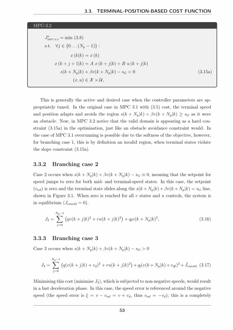
3.3. TERMINAL-POSITION-BASED COST FUNCTION
MPC-3.2
J∗MPC-3.2 = min (3.8)
s.t. ∀j ∈ 0 . . . (Np − 1) :
x (k|k) = x (k)
x (k + j + 1|k) = A x (k + j|k) +B u (k + j|k)
s(k +Np|k) + βv(k +Np|k)− sG < 0 (3.15a)
(x, u) ∈ X × U ,
This is generally the active and desired case when the controller parameters are ap-propriately tuned. In the original case in MPC 3.1 with (3.5) cost, the terminal speedand position adapts and avoids the region s(k + Np|k) + βv(k + Np|k) ≥ sG as it werean obstacle. Now, in MPC 3.2 notice that the valid domain is appearing as a hard con-straint (3.15a) in the optimisation, just like an obstacle avoidance constraint would. Inthe case of MPC 3.1 overrunning is possible due to the softness of the objective, however,for branching case 1, this is by definition an invalid region, when terminal states violatethe slope constraint (3.15a).
3.3.2 Branching case 2
Case 2 occurs when s(k +Np|k) + βv(k +Np|k)− sG ≡ 0, meaning that the setpoint forspeed jumps to zero for both mid- and terminal-speed states. In this case, the setpoint(vref) is zero and the terminal state slides along the s(k+Np|k) +βv(k+Np|k) = sG line,shown in Figure 3.1. When zero is reached for all v states and u controls, the system isin equilibrium (Jconst2 = 0).
J2 =
Np−1∑j=0
(qv(k + j|k)2 + ru(k + j|k)2
)+ qfv(k +Np|k)2, (3.16)
3.3.3 Branching case 3
Case 3 occurs when s(k +Np|k) + βv(k +Np|k)− sG > 0
J3 =
Np−1∑j=0
(q(v(k + j|k) + vd)
2 + ru(k + j|k)2)
+ qf(v(k+Np|k) + vdf )2 + Jconst3 (3.17)
Minimising this cost (minimise J3), which is subjected to non-negative speeds, would resultin a fast deceleration phase. In this case, the speed error is referenced around the negativespeed (the speed error is ξ = v − vref = v + vd, thus vref = −vd); this is a completely
53

CHAPTER 3. COST AND PREDICTIONS
Figure 3.1: The setpoint jumps between vd, 0 and −vd in line with the transition of s(k +Np|k) + βv(k +Np|k)− sG from a negative to a positive value.
unreachable setpoint, as it is in conflict with v ≥ 0 constraint (vref = −vd ≤ 0 ≤ v).Figure 3.1 shows the regions of respected cases of the l1-norm and the possible referencespeeds. It is forbidden and undesirable to have states of negative speeds or positionspassing through the goal corresponding to the grey areas in Figure 3.1. Switching betweenthe three possible cost cases opens the way to simplifying and modelling them as LQRcontrols with the choice to find stabilising tuning parameters. This makes it possible toform the appropriately tuned operating case, which results in a mathematical optimisationidentical to that of the ‘running-cost’ formulation with added terminal set constraints.
3.3.4 Tuning the controller
At this point, there are several parameters in the controller: q, r, qf, ρ and β. Furthermore,as previously identified, desired speed vd can be encompassed in the formulation thatappears as a reference speed in cases decided by an inherent switching of the terminalcost. The method for tuning entails choosing the stabilising linear control for the quadraticcost function. The three cases just discussed are reduced to LQR forms dependent onq, r and qf parameters, generally minimising the speed-state errors ξ = v − vref to thereference speed vref. For simplicity, let the setpoint vref be the same for each time step,making the general LQR form:
J =
Np−1∑j=0
(q ξ(k + j|k)2 + ru(k + j|k)2
)+ qf ξ(k +Np|k)2. (3.18)
Assume the following closed-loop control law:
u = −Kv (3.19)
54
3.3. TERMINAL-POSITION-BASED COST FUNCTION
where the closed loop gain is K and not yet determined. When the terminal state reachesthe desired surface defined by s + βv − sG = 0, it will ideally follow this surface untilreaching the equilibrium state at sG; this happens in case 2, where the l1 norm remains atzero. Thus, similarly to the positive invariance calculations, let the states coincide withs+ βv − sG = 0 line in two consecutive time steps:
sk + βvk − sG = sk+1 + βvk+1 − sG,
with substitution of:
sk+1 = sk + vkδt+ akδt2
2
vk+1 = vk + akδt
gives
vkδt+ akδt2
2+ βakδt = 0
ak = − 1δt2
+ βvk.
This defines the gain from (3.19):
K =1
δt2
+ β(3.20)
which can be used to calculate the q, r and qf parameters.The Discrete Algebraic Ricatti Equation (DARE) is:
ATQfA−Qf − ATQfB(BTQfB +R
)−1BTQfA+Q = 0,
where the positive LQR cost matrices are Q, R and Qf—which, in this formulation,are only one-dimensional (scalars)—and, respectively, the parameters q, r and qf. Fur-thermore, the optimal closed-loop gain is K =
(BTQfB +R
)−1BTQfA. The velocity
optimisation may be formulated exclusively through the use of speed states and controlinputs, as the positions are not utilised in the current unconstrained tuning; thus, thestate matrices are A = 1 and B = δt. The DARE simplifies to:
q = AT qfB K = qf K δt,
and the gain equation to
K =qfδt
qf δt2 + r.
55
CHAPTER 3. COST AND PREDICTIONS
Using the previously required gain setting to remain on the s+ βv − sG = 0 line:
qf =r(
1K− δt
)δt
=r(
β − δt2
)δt.
Furthermore, the scale of J in the LQR is arbitrary and can be chosen by fixing oneof the three parameters (q, r, or qf). For simplicity, let:
r ≡ 1,
qf =1(
β − δt2
)δt
q =1(
β − δt2
) (β + δt
2
) =1
β2 − δt2
4
.
(3.21)
To keep the parameters positive, β − δt2≥ 0; thus, similarly to the requirements in
Theorem 1, it is true that 0 ≤ δt ≤ 2β.
3.3.5 Stability
The three cases outlined above can be reduced to LQR controllers through which thereference speed is chosen by the terminal speed state and position prediction:
vref =
vd, s(k +Np|k) + βv(k +Np|k)− sG < 0, (Case 1)0, s(k +Np|k) + βv(k +Np|k)− sG ≡ 0, (Case 2)−vd, s(k +Np|k) + βv(k +Np|k)− sG > 0, (Case 3)
(3.22)
In case 3, the reference speed is unreachable because only positive speeds are allowed(i.e. in this framework, the vehicle cannot go to its goal position in reverse if it wasmissed). Case 2 has the stopping velocity profile with immediate deceleration due to thetuned LQR parameters, converging to an equilibrium state corresponding to vk→∞ = 0,uk→∞ = 0. However, if s(k + Np|k) ≤ sG and v(k + Np|k) = 0 then case 1 will beswitched to where vref = vd > 0; thus, the vehicle will be in motion at some point in thehorizon. If the terminal position s(k + Np|k) = sG or the terminal states are on the lineof s(k + Np|k) + βv(k + Np|k) − sG ≡ 0 then (since r > 0), the homogeneous penaltyover all control inputs in the horizon ensures that the acceleration to reach the goal isspread across the time horizon. This is important because doing so results in some degreeof initial acceleration v(k + 1|k) > 0, meaning that no idling or loitering happens in thefinite horizon (otherwise, v = 0 sections could form). Furthermore, the vehicle wouldbuild up speed even if it had been stationary (i.e. v(k) = 0), for example, after a fullstop before a junction. Finally, v(k + 1|k) > 0 ensures that s(k + 1) increases over s(k)
when s(k) + βv(k) < sG (i.e. the vehicle starts moving towards the goal position, ergothe equilibrium state).
56
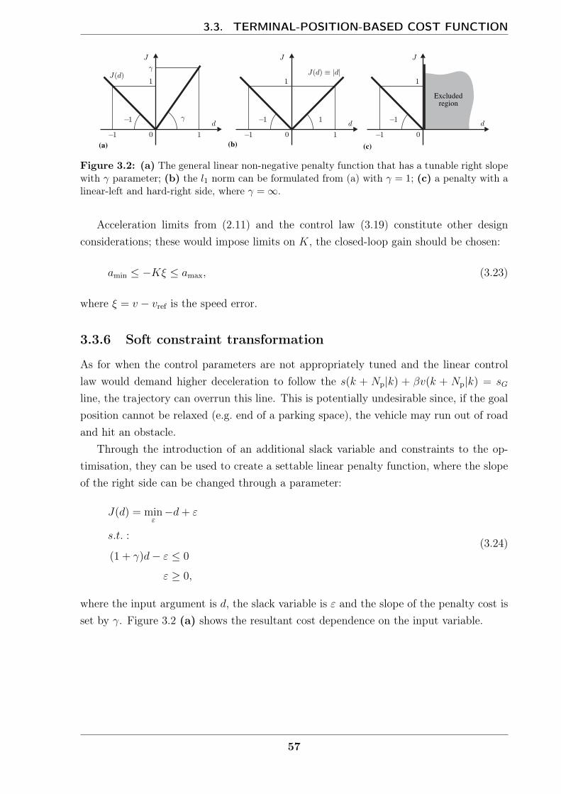
3.3. TERMINAL-POSITION-BASED COST FUNCTION
Figure 3.2: (a) The general linear non-negative penalty function that has a tunable right slopewith γ parameter; (b) the l1 norm can be formulated from (a) with γ = 1; (c) a penalty with alinear-left and hard-right side, where γ =∞.
Acceleration limits from (2.11) and the control law (3.19) constitute other designconsiderations; these would impose limits on K, the closed-loop gain should be chosen:
amin ≤ −Kξ ≤ amax, (3.23)
where ξ = v − vref is the speed error.
3.3.6 Soft constraint transformation
As for when the control parameters are not appropriately tuned and the linear controllaw would demand higher deceleration to follow the s(k + Np|k) + βv(k + Np|k) = sG
line, the trajectory can overrun this line. This is potentially undesirable since, if the goalposition cannot be relaxed (e.g. end of a parking space), the vehicle may run out of roadand hit an obstacle.
Through the introduction of an additional slack variable and constraints to the op-timisation, they can be used to create a settable linear penalty function, where the slopeof the right side can be changed through a parameter:
J(d) = minε−d+ ε
s.t. :
(1 + γ)d− ε ≤ 0
ε ≥ 0,
(3.24)
where the input argument is d, the slack variable is ε and the slope of the penalty cost isset by γ. Figure 3.2 (a) shows the resultant cost dependence on the input variable.
57

CHAPTER 3. COST AND PREDICTIONS
Notice that the l1 norm can be decomposed in the previous form when γ = 1:
|d| = J(d) = minε−d+ ε
s.t. :
2d− ε ≤ 0
ε ≥ 0
which is shown in Figure 3.2 (b).Recall that the original cost analysed in (3.5) sets the reference speed (3.22) in case 3
to negative for the LQR form (i.e. vref = −vd = −ρδt2q). However, this can be arbitrarily
changed when the generalised soft-penalty formulation from (3.24) is being implementedwith the γ parameter. Softened constraints are beneficial because their violation is feas-ible; thus, the controller may operate even after, for example, inadvertently passing thegoal position. It is possible to choose the parameter tuning with l1 and l∞ norm softpenalties to give back the feasible hard-constraint-equivalent optimal trajectories usingthe exact penalty method [41] or approximate l2 penalty function cases. In this case,the design considerations allow the controller to operate without entering case 3, whichotherwise would necessitate the soft penalty formulation.
However, this work does not focus on softening obstacle avoidance constraints; bychoosing the soft-constraint penalty γ to∞, or fixing ε = 0 and eliminating the softening,case 3 is made a forbidden region. A hard-constraint case is shown in Figure 3.2 (c).This keeps the operating modes in cases 1 and 2 attainable but requires positive control-invariant consideration for the terminal set to remain recursively feasible. Thus, it is theadditional hard constraint that retains the form:
d ≤ 0.
By substitution of the original l1-norm argument in place of d gives:
s(k +Np|k) + βv(k +Np|k)− sG ≤ 0
hard constraint and
β − δt
2≥ 0,
β +δt
2=
1
K≤ −vmax
amin
requirements.
58

3.3. TERMINAL-POSITION-BASED COST FUNCTION
3.3.7 Numerical examples
This section highlights the properties of the controllers discussed previously. The twoMPC formulations are the soft formulation, MPC 3.3, with the terminal-position-basedcost, and the hard formulation, MPC 3.4, with the ‘running-cost’ and hard constraintcondition. When tuned appropriately the two MPCs are expected to generate identicaltrajectories for unconstrained cases (disabled speed and acceleration limits). Moreover,in constrained cases where the test problems are set up to induce constraint violations,the soft formulation is expected to remain feasible, in contrast to the hard ‘running-cost’formulation, which is expected to become infeasible on hard constrain violation.
The soft formulation, MPC 3.3, is defined without the state (speed) limits (3.25b) andcontrol input limits (3.25c). MPC 3.3 is:
MPC-3.3, MPC formulation with l1-norm based terminal-cost
J∗MPC-3.3 = min
Np−1∑j=0
(qv(k + j|k)2 + ru(k + j|k)2
)+ qfv(k +Np|k)2
+ ρ |s(k +Np|k) + βv(k +Np|k)− sG| (3.25a)
s.t. ∀j ∈ 0 . . . (Np − 1) :
x (k|k) = x (k)
x (k + j + 1|k) = A x (k + j|k) +B u (k + j|k)
v(k + j + 1|k) ≥ 0
XXXXx ∈ X (3.25b)
XXXXu ∈ U (3.25c)
The hard ‘running-cost’ formulation is MPC 3.4 subject to only the equalities of thedynamics and the hard constraint (3.26d) with similarly disabled speed limits (3.26b) andcontrol input limits (3.26c):
59

CHAPTER 3. COST AND PREDICTIONS
MPC-3.4, MPC formulation with ‘running-cost’ and hard constraint
J∗MPC-3.4 = min
Np−1∑j=0
(qξ(k + j|k)2 + ru(k + j|k)2
)+ qfξ(k +Np|k)2 (3.26a)
s.t. ∀j ∈ 0 . . . (Np − 1) :
x (k|k) = x (k)
x (k + j + 1|k) = A x (k + j|k) +B u (k + j|k)
v(k + j + 1|k) ≥ 0
XXXXx ∈ X (3.26b)
XXXXu ∈ U (3.26c)
s(k +Np|k) + βv(k +Np|k)− sG ≤ 0, (3.26d)
where the speed errors are ξ(k + j|k) = v(k + j|k)− vd.Note that the following experiments are only for demonstration purposes obtaining
the unconstrained trajectories, as the formulations would naturally behave without theoperational state and control limits defined, while initial states of the simulation are stillchosen within the state limits to correspond with relevant cases.
The first simulation parameters are δt = 0.5 s, Np = 1, sG = 0 m, vd = 9 ms−1 andx(0) = [−100, 8]T with initial position and speed in m and ms−1, respectively. Parametersq, r, qf and ρ were chosen with β = 3.4197 s from (3.21). Furthermore, the limits,if they would have been imposed, were amax = 9.81/4 ms−2, amin = −9.81/2 ms−2 andvmax = 10 ms−1. The modelling was done using CVX, a package for specifying and solvingconvex programs in Matlab [16, 28].
In Figure 3.3 (a), the trajectories of the two MPCs can be seen coinciding as expected.In the first section, both controllers approach the vd reference speed. Later, a slowdownperiod can be seen respecting the chosen 1/β slope on the v–s graph converging towardsthe goal position. The shown accelerations in Figure 3.3 (b) have monotonic decreasingtrends after the initial tracking error and the switch to goal approaching phase. In Fig-ure 3.4, the optimal cost of MPC 3.3 goes to zero (i.e. J([sG, 0]) ≡ 0) in contrast with
(a)-100 -80 -60 -40 -20 0
s [m]
0
2
4
6
8
10
v [
m/s
]
MPC1 tail
MPC1 traj
MPC2 tail
MPC2 traj
vd
(v lims)
(b)0 10 20 30 40 50
k [-]
-6
-4
-2
0
2
4
u [
m/s
2]
u (MPC1)
u (MPC2)
(u lims)
Figure 3.3: Comparison of the two MPC controller formulations: MPC 3.3 (MPC1) andMPC 3.4 (MPC2) (a) v–s and (b) u–k.
60
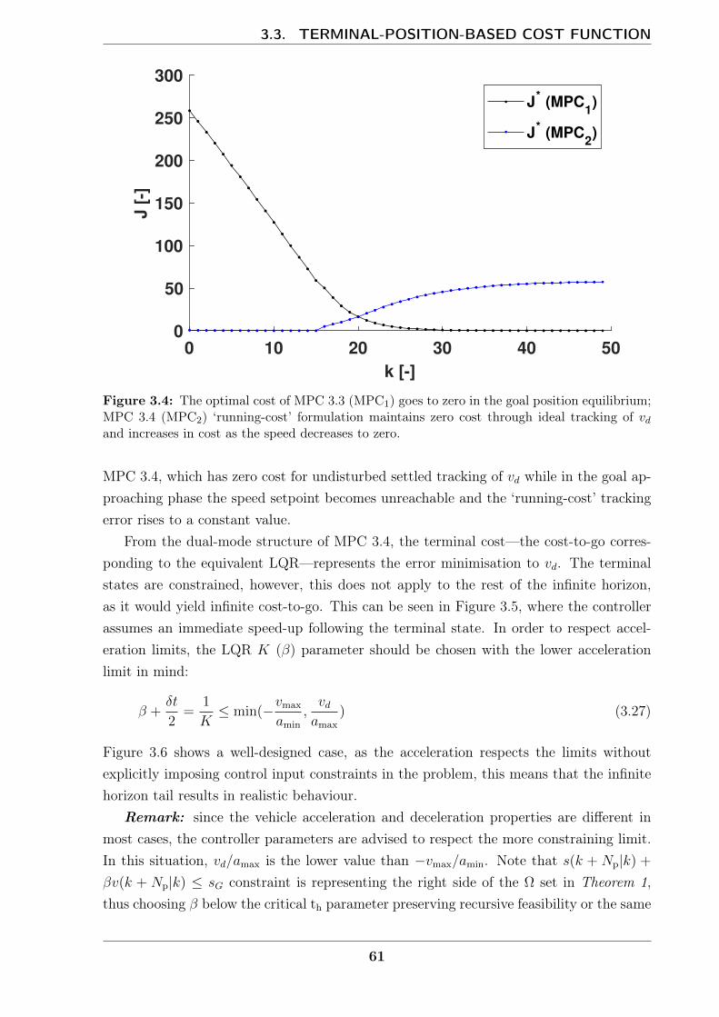
3.3. TERMINAL-POSITION-BASED COST FUNCTION
0 10 20 30 40 50
k [-]
0
50
100
150
200
250
300
J [
-]
J* (MPC
1)
J* (MPC
2)
Figure 3.4: The optimal cost of MPC 3.3 (MPC1) goes to zero in the goal position equilibrium;MPC 3.4 (MPC2) ‘running-cost’ formulation maintains zero cost through ideal tracking of vdand increases in cost as the speed decreases to zero.
MPC 3.4, which has zero cost for undisturbed settled tracking of vd while in the goal ap-proaching phase the speed setpoint becomes unreachable and the ‘running-cost’ trackingerror rises to a constant value.
From the dual-mode structure of MPC 3.4, the terminal cost—the cost-to-go corres-ponding to the equivalent LQR—represents the error minimisation to vd. The terminalstates are constrained, however, this does not apply to the rest of the infinite horizon,as it would yield infinite cost-to-go. This can be seen in Figure 3.5, where the controllerassumes an immediate speed-up following the terminal state. In order to respect accel-eration limits, the LQR K (β) parameter should be chosen with the lower accelerationlimit in mind:
β +δt
2=
1
K≤ min(−vmax
amin
,vdamax
) (3.27)
Figure 3.6 shows a well-designed case, as the acceleration respects the limits withoutexplicitly imposing control input constraints in the problem, this means that the infinitehorizon tail results in realistic behaviour.
Remark: since the vehicle acceleration and deceleration properties are different inmost cases, the controller parameters are advised to respect the more constraining limit.In this situation, vd/amax is the lower value than −vmax/amin. Note that s(k + Np|k) +
βv(k + Np|k) ≤ sG constraint is representing the right side of the Ω set in Theorem 1,thus choosing β below the critical th parameter preserving recursive feasibility or the same
61
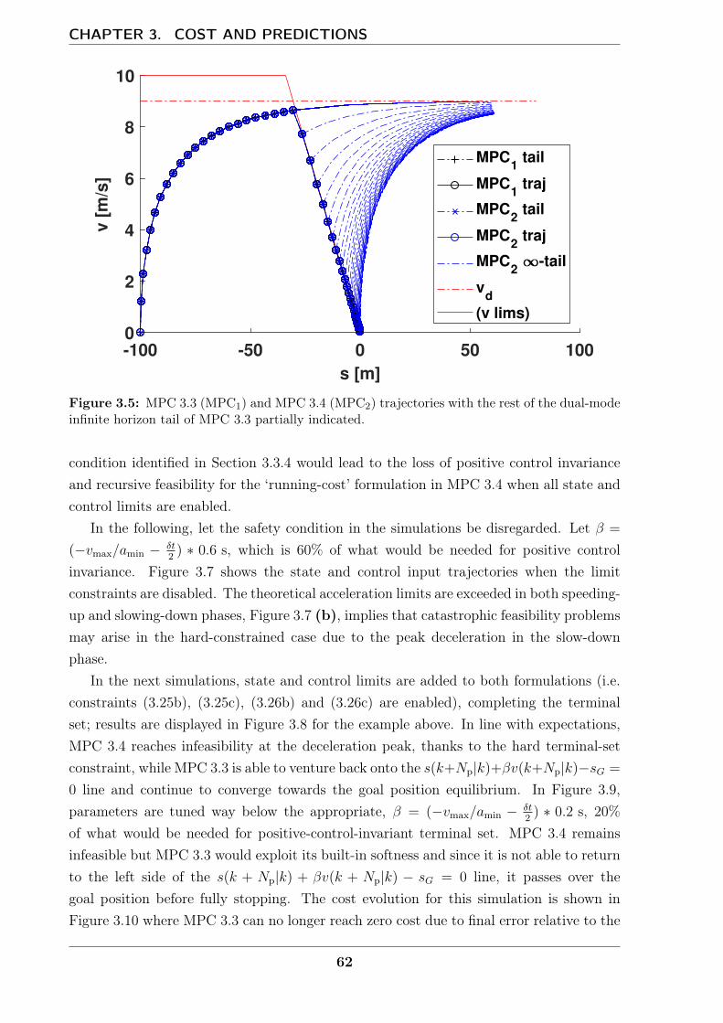
CHAPTER 3. COST AND PREDICTIONS
-100 -50 0 50 100
s [m]
0
2
4
6
8
10
v [
m/s
]
MPC1 tail
MPC1 traj
MPC2 tail
MPC2 traj
MPC2 -tail
vd
(v lims)
Figure 3.5: MPC 3.3 (MPC1) and MPC 3.4 (MPC2) trajectories with the rest of the dual-modeinfinite horizon tail of MPC 3.3 partially indicated.
condition identified in Section 3.3.4 would lead to the loss of positive control invarianceand recursive feasibility for the ‘running-cost’ formulation in MPC 3.4 when all state andcontrol limits are enabled.
In the following, let the safety condition in the simulations be disregarded. Let β =
(−vmax/amin − δt2
) ∗ 0.6 s, which is 60% of what would be needed for positive controlinvariance. Figure 3.7 shows the state and control input trajectories when the limitconstraints are disabled. The theoretical acceleration limits are exceeded in both speeding-up and slowing-down phases, Figure 3.7 (b), implies that catastrophic feasibility problemsmay arise in the hard-constrained case due to the peak deceleration in the slow-downphase.
In the next simulations, state and control limits are added to both formulations (i.e.constraints (3.25b), (3.25c), (3.26b) and (3.26c) are enabled), completing the terminalset; results are displayed in Figure 3.8 for the example above. In line with expectations,MPC 3.4 reaches infeasibility at the deceleration peak, thanks to the hard terminal-setconstraint, while MPC 3.3 is able to venture back onto the s(k+Np|k)+βv(k+Np|k)−sG =
0 line and continue to converge towards the goal position equilibrium. In Figure 3.9,parameters are tuned way below the appropriate, β = (−vmax/amin − δt
2) ∗ 0.2 s, 20%
of what would be needed for positive-control-invariant terminal set. MPC 3.4 remainsinfeasible but MPC 3.3 would exploit its built-in softness and since it is not able to returnto the left side of the s(k + Np|k) + βv(k + Np|k) − sG = 0 line, it passes over thegoal position before fully stopping. The cost evolution for this simulation is shown inFigure 3.10 where MPC 3.3 can no longer reach zero cost due to final error relative to the
62
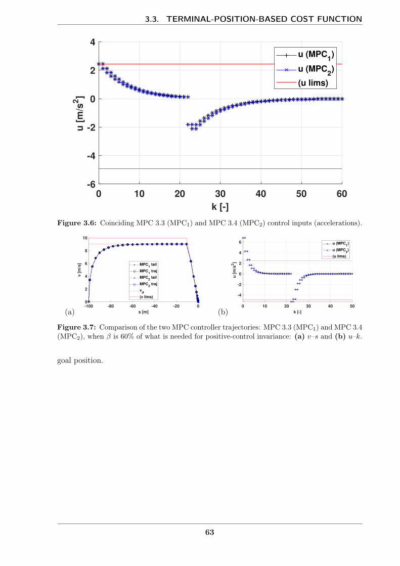
3.3. TERMINAL-POSITION-BASED COST FUNCTION
0 10 20 30 40 50 60
k [-]
-6
-4
-2
0
2
4
u [
m/s
2]
u (MPC1)
u (MPC2)
(u lims)
Figure 3.6: Coinciding MPC 3.3 (MPC1) and MPC 3.4 (MPC2) control inputs (accelerations).
(a)-100 -80 -60 -40 -20 0
s [m]
0
2
4
6
8
10
v [
m/s
] MPC1 tail
MPC1 traj
MPC2 tail
MPC2 traj
vd
(v lims)
(b)0 10 20 30 40 50
k [-]
-4
-2
0
2
4
6
u [
m/s
2]
u (MPC1)
u (MPC2)
(u lims)
Figure 3.7: Comparison of the two MPC controller trajectories: MPC 3.3 (MPC1) and MPC 3.4(MPC2), when β is 60% of what is needed for positive-control invariance: (a) v–s and (b) u–k.
goal position.
63
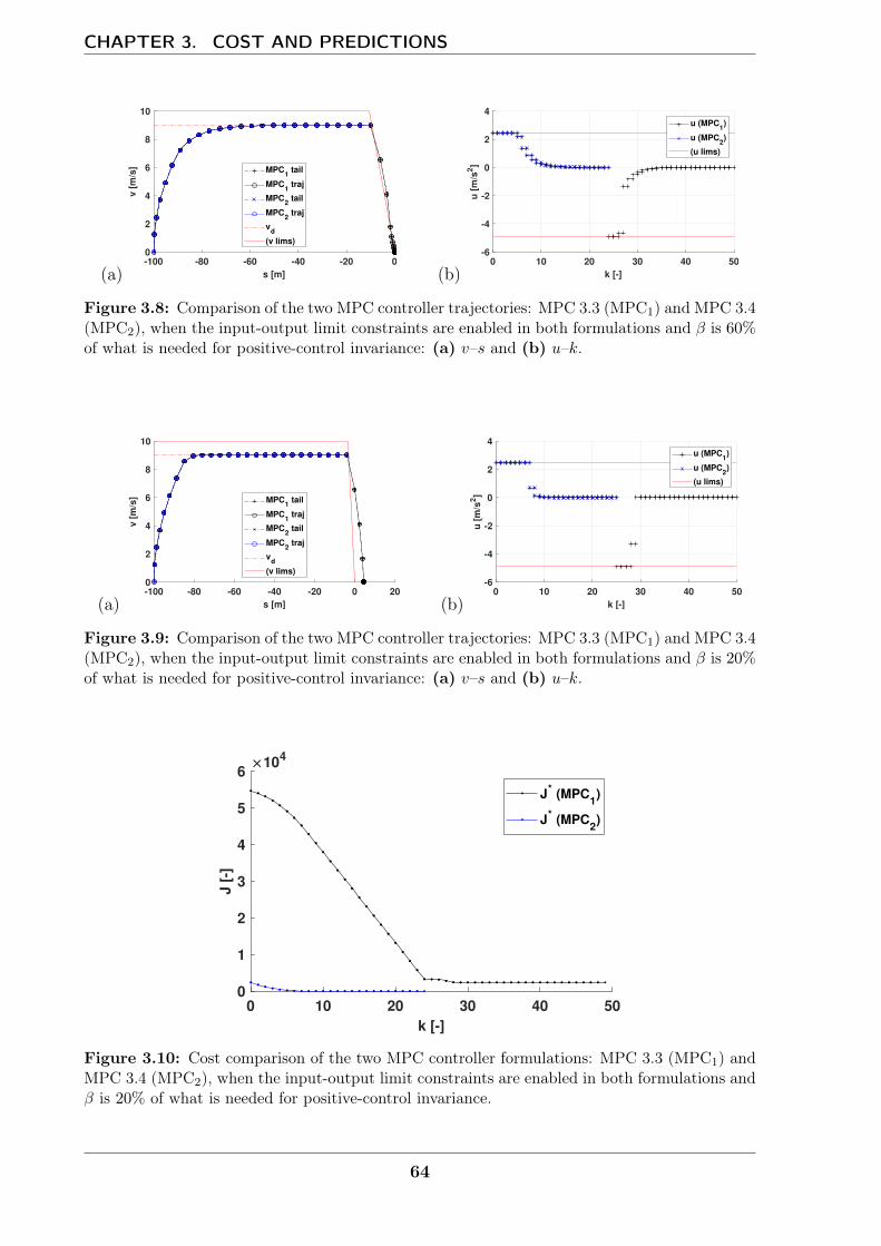
CHAPTER 3. COST AND PREDICTIONS
(a)-100 -80 -60 -40 -20 0
s [m]
0
2
4
6
8
10
v [
m/s
] MPC1 tail
MPC1 traj
MPC2 tail
MPC2 traj
vd
(v lims)
(b)0 10 20 30 40 50
k [-]
-6
-4
-2
0
2
4
u [
m/s
2]
u (MPC1)
u (MPC2)
(u lims)
Figure 3.8: Comparison of the two MPC controller trajectories: MPC 3.3 (MPC1) and MPC 3.4(MPC2), when the input-output limit constraints are enabled in both formulations and β is 60%of what is needed for positive-control invariance: (a) v–s and (b) u–k.
(a)-100 -80 -60 -40 -20 0 20
s [m]
0
2
4
6
8
10
v [
m/s
] MPC1 tail
MPC1 traj
MPC2 tail
MPC2 traj
vd
(v lims)
(b)0 10 20 30 40 50
k [-]
-6
-4
-2
0
2
4
u [
m/s
2]
u (MPC1)
u (MPC2)
(u lims)
Figure 3.9: Comparison of the two MPC controller trajectories: MPC 3.3 (MPC1) and MPC 3.4(MPC2), when the input-output limit constraints are enabled in both formulations and β is 20%of what is needed for positive-control invariance: (a) v–s and (b) u–k.
0 10 20 30 40 50
k [-]
0
1
2
3
4
5
6
J [
-]
104
J* (MPC
1)
J* (MPC
2)
Figure 3.10: Cost comparison of the two MPC controller formulations: MPC 3.3 (MPC1) andMPC 3.4 (MPC2), when the input-output limit constraints are enabled in both formulations andβ is 20% of what is needed for positive-control invariance.
64
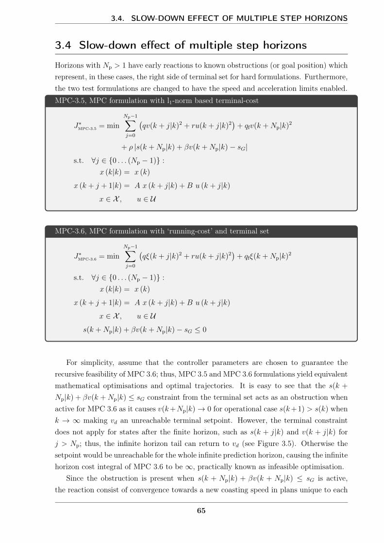
3.4. SLOW-DOWN EFFECT OF MULTIPLE STEP HORIZONS
3.4 Slow-down effect of multiple step horizons
Horizons with Np > 1 have early reactions to known obstructions (or goal position) whichrepresent, in these cases, the right side of terminal set for hard formulations. Furthermore,the two test formulations are changed to have the speed and acceleration limits enabled.MPC-3.5, MPC formulation with l1-norm based terminal-cost
J∗MPC-3.5 = min
Np−1∑j=0
(qv(k + j|k)2 + ru(k + j|k)2
)+ qfv(k +Np|k)2
+ ρ |s(k +Np|k) + βv(k +Np|k)− sG|
s.t. ∀j ∈ 0 . . . (Np − 1) :
x (k|k) = x (k)
x (k + j + 1|k) = A x (k + j|k) +B u (k + j|k)
x ∈ X , u ∈ U
MPC-3.6, MPC formulation with ‘running-cost’ and terminal set
J∗MPC-3.6 = min
Np−1∑j=0
(qξ(k + j|k)2 + ru(k + j|k)2
)+ qfξ(k +Np|k)2
s.t. ∀j ∈ 0 . . . (Np − 1) :
x (k|k) = x (k)
x (k + j + 1|k) = A x (k + j|k) +B u (k + j|k)
x ∈ X , u ∈ U
s(k +Np|k) + βv(k +Np|k)− sG ≤ 0
For simplicity, assume that the controller parameters are chosen to guarantee therecursive feasibility of MPC 3.6; thus, MPC 3.5 and MPC 3.6 formulations yield equivalentmathematical optimisations and optimal trajectories. It is easy to see that the s(k +
Np|k) + βv(k +Np|k) ≤ sG constraint from the terminal set acts as an obstruction whenactive for MPC 3.6 as it causes v(k+Np|k)→ 0 for operational case s(k+1) > s(k) whenk → ∞ making vd an unreachable terminal setpoint. However, the terminal constraintdoes not apply for states after the finite horizon, such as s(k + j|k) and v(k + j|k) forj > Np; thus, the infinite horizon tail can return to vd (see Figure 3.5). Otherwise thesetpoint would be unreachable for the whole infinite prediction horizon, causing the infinitehorizon cost integral of MPC 3.6 to be ∞, practically known as infeasible optimisation.
Since the obstruction is present when s(k + Np|k) + βv(k + Np|k) ≤ sG is active,the reaction consist of convergence towards a new coasting speed in plans unique to each
65
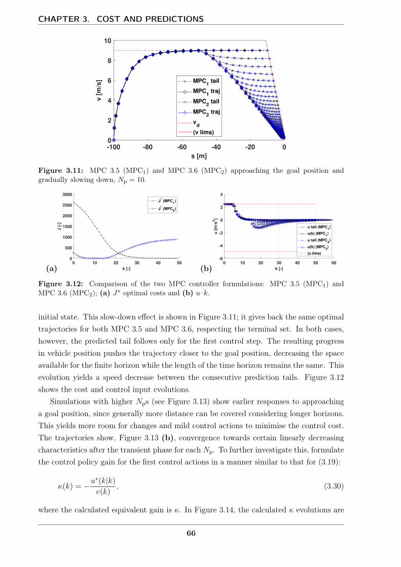
CHAPTER 3. COST AND PREDICTIONS
-100 -80 -60 -40 -20 0
s [m]
0
2
4
6
8
10
v [
m/s
] MPC1 tail
MPC1 traj
MPC2 tail
MPC2 traj
vd
(v lims)
Figure 3.11: MPC 3.5 (MPC1) and MPC 3.6 (MPC2) approaching the goal position andgradually slowing down, Np = 10.
(a)0 10 20 30 40 50
k [-]
0
500
1000
1500
2000
2500
3000
J [
-]
J* (MPC
1)
J* (MPC
2)
(b)0 10 20 30 40 50 60
k [-]
-6
-4
-2
0
2
4
u [
m/s
2]
u tail (MPC1)
u(k) (MPC1)
u tail (MPC2)
u(k) (MPC2)
(u lims)
Figure 3.12: Comparison of the two MPC controller formulations: MPC 3.5 (MPC1) andMPC 3.6 (MPC2); (a) J∗ optimal costs and (b) u–k.
initial state. This slow-down effect is shown in Figure 3.11; it gives back the same optimaltrajectories for both MPC 3.5 and MPC 3.6, respecting the terminal set. In both cases,however, the predicted tail follows only for the first control step. The resulting progressin vehicle position pushes the trajectory closer to the goal position, decreasing the spaceavailable for the finite horizon while the length of the time horizon remains the same. Thisevolution yields a speed decrease between the consecutive prediction tails. Figure 3.12shows the cost and control input evolutions.
Simulations with higher Nps (see Figure 3.13) show earlier responses to approachinga goal position, since generally more distance can be covered considering longer horizons.This yields more room for changes and mild control actions to minimise the control cost.The trajectories show, Figure 3.13 (b), convergence towards certain linearly decreasingcharacteristics after the transient phase for each Np. To further investigate this, formulatethe control policy gain for the first control actions in a manner similar to that for (3.19):
κ(k) = −u∗(k|k)
v(k), (3.30)
where the calculated equivalent gain is κ. In Figure 3.14, the calculated κ evolutions are
66

3.4. SLOW-DOWN EFFECT OF MULTIPLE STEP HORIZONS
(a)0 20 40 60 80 100
k [-]
-200
-150
-100
-50
0
s [
m]
Np=1
Np=10
Np=30
(b)-200 -150 -100 -50 0
s [m]
0
2
4
6
8
10
v [
m/s
]
Np=1
Np=10
Np=30
(v lims)
Figure 3.13: (a) s–k and (b) v–s graphs for goal-approaching simulation with Np = 1, 10, 30horizons.
shown for goal approach simulations; their respective trajectories are shown in Figure 3.13.In the case of Np = 1, the design gain of the terminal set from the β headway time and δtcontrol period time (3.20) is attained because the horizon has no information about theobstruction presented by the terminal constraints until they are reached and activated. κremains more moderate for higher horizon lengths than short horizons practically limitedby the design of the terminal set. Moreover, the control action is applied sooner and tendsto converge after a transient phase. A set of horizon lengths are tested where κ values atthe end of the simulations are sampled and assumed to be sufficiently converged (close tostop). These κ values are used to calculate control-period-normalised time headways:
β
δt=
1
κδt− 1
2(3.31)
which are shown in Figure 3.15. Note that, for a low number of horizon steps, theformulation ensures safety by limiting the rate of slow-down through the original β designparameter to safe levels as proved by the converged trends of slow-down trajectories. Thislimiting effect can be seen in Figure 3.15 as the β
δtline. For longer horizons, the trajectory
profiles converge to the normalised time headway corresponding to Np − 12. This shows
that with the tuning choices, longer horizons are able to accommodate longer slow-downtrajectories to static obstacles or goal positions, inherently respecting control limits, andshort horizon formulations are actively benefiting from the safety design choices in theframework.
67

CHAPTER 3. COST AND PREDICTIONS
0 20 40 60 80 100
k [-]
0
0.05
0.1
0.15
0.2
0.25
0.3
[1
/s]
Np=1
Np=10
Np=30
K( , t)
Figure 3.14: The evolution of κ gain for goal-approaching simulation with Np = 1, 10, 30horizons.
10 20 30 40 50
Np [-]
0
10
20
30
40
Figure 3.15: The converged and normalised time headway initially follows the design gain ofthe terminal set for short horizons but switches over to the empirical Np − 1/2 horizon length-dependent line for longer horizons.
68
3.5. TWO-VEHICLE PRE-MERGING
3.5 Two-vehicle pre-merging
In the case of car-following, the vehicles have the previously discussed (Section 2.3.4)separation requirement formulated as a hard constraint. When two vehicles merge orpass through junctions, their hard separation constraints are active or relaxed in the MIPformulation to preserve safety (Section 2.5). If a cost were to be assigned to a hardconstraint then when it is not violated its penalty cost would be zero, when it is violatedits penalty cost would be infinite. It stands to reason that this sudden jump could bemade smoother, potentially preparing for future obstacles and conflict zones ahead oftime. As shown in Section 3.4, the slow-down effect of a longer horizon result in thepotential for an earlier reaction in response to an obstruction. This yields mild, lessintensive control actions to achieve the output requirements (e.g. deceleration before anobstacle or in merging creating the appropriate separation for car-following). It would becomputationally demanding to simply increase the length of the horizon, thus, anotherapproach will be explored. In this section, an additional cost element is formulatedthat softly encompasses and adds the vehicle-separation constraint of the merging to theobjective function.
For simplicity, let the aggregated cost function for a restricted case be investigatedwith two vehicles a and b:
J = σFsep(xa (k +Np|k) , xb (k +Np|k)) +∑
n∈a,b
wnF (xn (k +Np|k))
+
Np−1∑j=0
wnln (xn (k + j|k) , un (k + j|k)) , (3.32)
where stage cost is ln = q (vn − vd n)2+r u2n, the relative weights are wn, and the terminalcost is F = qf (v − vd)2. Moreover, the weight for the soft separation penalty is σ andthe soft separation penalty is:
Fsep = sb(k +Np − 1|k)− sa(k +Np|k)− βva(k +Np|k)− L
where the index of the leader vehicle is b and the safe car-following separation gap hasyet to be achieved; thus, sb(k+Np− 1|k)− sa(k+Np|k)− βva(k+Np|k)−L ≥ 0 and, assuch, Fsep ≥ 0. Later, this formulation is generalised for the whole scenario with arbitraryvehicle positions. Let the positions be reformulated with the use of the speed decisionvariables with the help of (3.9):
Fsep = sb(k)− sa(k)− L+ vb(k)δt
2− va(k)
δt
2+ vb(k + 1|k)δt− va(k + 1|k)δt
+ . . .+ vb(k +Np − 1|k)δt
2− va(k +Np − 1|k)δt− va(k +Np|k)
(δt
2+ β
)
69

CHAPTER 3. COST AND PREDICTIONS
Following the arguments in Section 3.2, the constants can be disregarded in the optim-isation (e.g. sb(k)− sa(k)−L+ vb(k) δt
2− va(k) δt
2). Therefore, what remains are linearly
dependent speed terms that amend the originally desired vehicle speeds through weight-ing. The desired speeds are ordered in vector forms for better representation where theelements are desired speed to be considered in stage costs and the terminal speed atk, k + 1, . . . , Np − 1, k +Np.
vd a =
[vd a −
σδt
2waq, vd a −
σδt
2waq, . . . , vd a −
σδt
2waq, vd a −
σ(δt2
+ β)
2waqf
]T,
vd b =
[vd b +
σδt
2wbq, vd b +
σδt
2wbq, . . . , vd b +
σδt
4wbq, vd b
]TIt should be noted that the desired speed for first time step (k) is arbitrary since the speedstate is a fixed value v(k|k) = v(k), thus, as a constant shift it may be also disregarded inthe optimisation. Moreover, the leader vehicle has its desired speed increased for (Np ≥ 2)horizons while the follower vehicle has its speed decreased for all valid horizons (Np ≥ 1)with the terminal desired speed having a change compared to that at the middle of thehorizon. This would mean that in the case of Np = 1, the leader vehicle experiences nochange in its cost and makes no effort to cooperate with the follower vehicle (Figure 3.16).
Moreover, this formulation would cause the desired speeds to be changed even afterthe desired separation is achieved (see Figure 3.16). Formulating it as a true soft penalty,the cost can be deactivated when the intended separation is reached.MPC-3.7
J∗MPC-3.7 = min σFsep +∑
n∈a,b
wnF (xn (k +Np|k))
+
Np−1∑j=0
wnln (xn (k + j|k) , un (k + j|k))
s.t. ∀j ∈ 0 . . . (Np − 1), ∀n ∈ a, b :
xn (k|k) = xn (k)
xn (k + j + 1|k) = A xn (k + j|k) +B un (k + j|k)
xn ∈ Xnun ∈ Un
sa(k +Np|k) + βva(k +Np|k)− sb(k +Np − 1|k) + L− Fsep ≤ 0 (3.33a)
Fsep ≥ 0 (3.33b)
When the soft separation cost is inserted into the merging scenario, it is beneficial tosee that the car-following modes utilise the same hyperplane. Practically, it is a linear
70
3.5. TWO-VEHICLE PRE-MERGING
soft penalty version of the later-appearing hard constraints promoting a softer transitionbetween the approaching and car-following modes. When the states reach the hard car-following constraints of the same kind this Fsep cost would turn to zero and vanish fromthe optimisation. σ weight sets the intensity of the earlier response while the timelinessof completion depends on the intensity as well. This means that late information may notlead to significantly different trajectories while too soon knowledge would yield the samefixed rate of trajectory change. In the simplest case of two-vehicle merging, this cost hasto be defined for both vehicle orders and, with the already existing binaries, the extrapenalty terms may be relaxed just like a hard constraint would.
J = σ (Fsep ab + Fsep ba) +∑
n∈a,b
wnF (xn (k +Np|k))
+
Np−1∑j=0
wnln (xn (k + j|k) , un (k + j|k)) , (3.34)
Furthermore, the additional constraints are:
sa(k +Np|k) + βva(k +Np|k)− sb(k +Np − 1|k)+L− Fsep ab
≤M b1(k +Np|k) (3.35a)
sb(k +Np|k) + βvb(k +Np|k)− sa(k +Np − 1|k)+L− Fsep ba
≤M b2(k +Np|k) (3.35b)
Fsep ab ≥ 0, (3.35c)
Fsep ba ≥ 0, (3.35d)
where the binary variable connected to obstacle-approaching mode in merging is b1(k +
Np|k) for vehicle a (which mode is active for b1(k +Np|k) ≡ 0 ) and similarly the binaryvariable connected to obstacle-approaching mode in merging is b2(k + Np|k) for vehicleb (which mode is active for b2(k + Np|k) ≡ 0). The obstacle-avoidance constraints andtheir handover for merging were discussed in Section 2.5; the corner-cutting preventionwas discussed in Section 2.3.5.1.
71
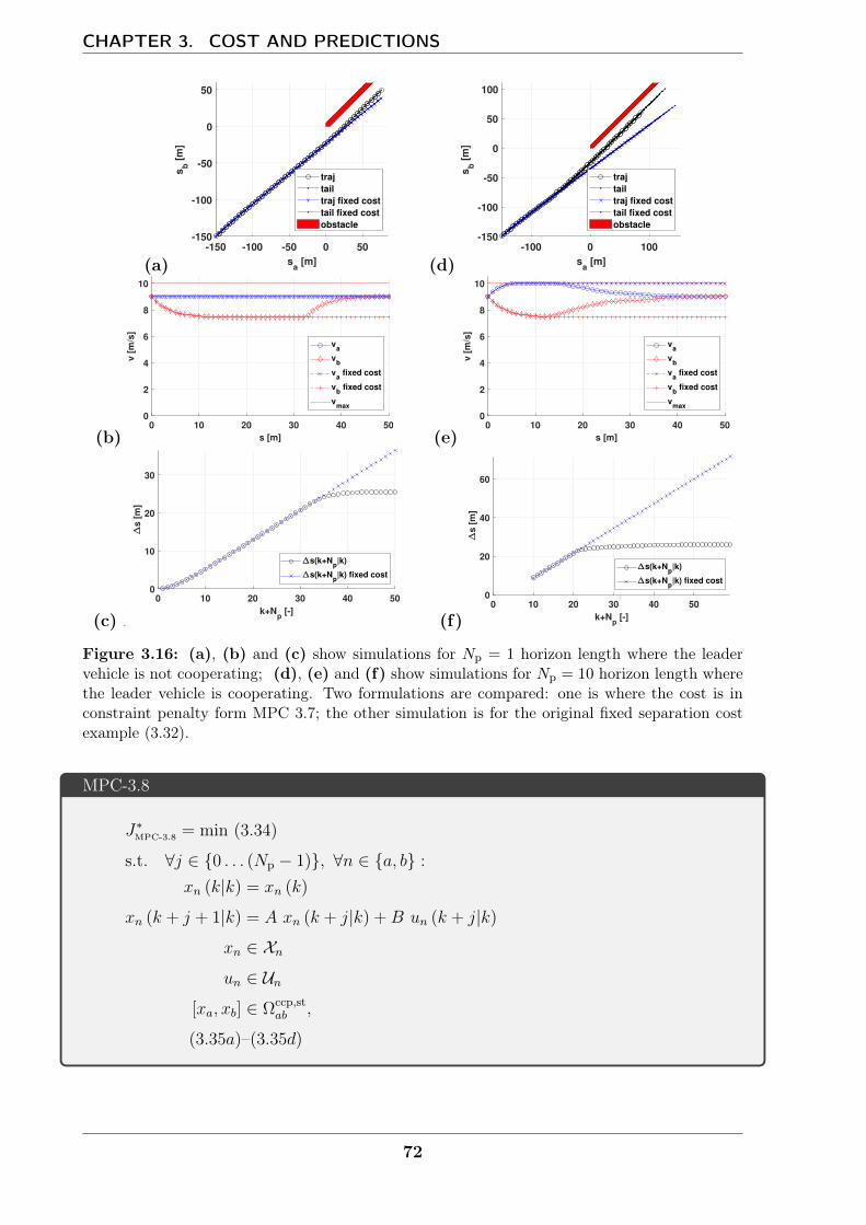
CHAPTER 3. COST AND PREDICTIONS
(a)-150 -100 -50 0 50
sa [m]
-150
-100
-50
0
50
sb [
m]
traj
tail
traj fixed cost
tail fixed cost
obstacle
(d)-100 0 100
sa [m]
-150
-100
-50
0
50
100
sb [
m]
traj
tail
traj fixed cost
tail fixed cost
obstacle
(b)0 10 20 30 40 50
s [m]
0
2
4
6
8
10
v [
m/s
]
va
vb
va fixed cost
vb fixed cost
vmax
(e)0 10 20 30 40 50
s [m]
0
2
4
6
8
10
v [
m/s
]
va
vb
va fixed cost
vb fixed cost
vmax
(c)0 10 20 30 40 50
k+Np [-]
0
10
20
30
s [
m]
s(k+Np|k)
s(k+Np|k) fixed cost
(f)0 10 20 30 40 50
k+Np [-]
0
20
40
60s
[m
]
s(k+Np|k)
s(k+Np|k) fixed cost
Figure 3.16: (a), (b) and (c) show simulations for Np = 1 horizon length where the leadervehicle is not cooperating; (d), (e) and (f) show simulations for Np = 10 horizon length wherethe leader vehicle is cooperating. Two formulations are compared: one is where the cost is inconstraint penalty form MPC 3.7; the other simulation is for the original fixed separation costexample (3.32).
MPC-3.8
J∗MPC-3.8 = min (3.34)
s.t. ∀j ∈ 0 . . . (Np − 1), ∀n ∈ a, b :
xn (k|k) = xn (k)
xn (k + j + 1|k) = A xn (k + j|k) +B un (k + j|k)
xn ∈ Xnun ∈ Un
[xa, xb] ∈ Ωccp,stab ,
(3.35a)–(3.35d)
72
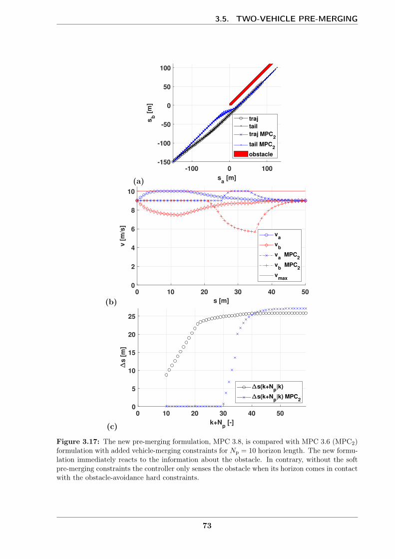
3.5. TWO-VEHICLE PRE-MERGING
(a)
-100 0 100
sa [m]
-150
-100
-50
0
50
100
sb [
m]
traj
tail
traj MPC2
tail MPC2
obstacle
(b)0 10 20 30 40 50
s [m]
0
2
4
6
8
10
v [
m/s
]
va
vb
va MPC
2
vb MPC
2
vmax
(c)
0 10 20 30 40 50
k+Np [-]
0
5
10
15
20
25
s [
m]
s(k+Np|k)
s(k+Np|k) MPC
2
Figure 3.17: The new pre-merging formulation, MPC 3.8, is compared with MPC 3.6 (MPC2)formulation with added vehicle-merging constraints for Np = 10 horizon length. The new formu-lation immediately reacts to the information about the obstacle. In contrary, without the softpre-merging constraints the controller only senses the obstacle when its horizon comes in contactwith the obstacle-avoidance hard constraints.
73
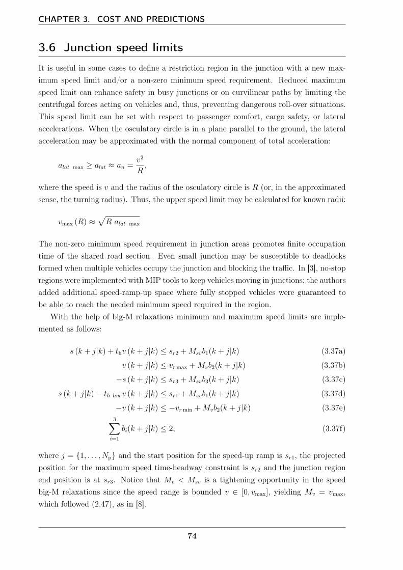
CHAPTER 3. COST AND PREDICTIONS
3.6 Junction speed limits
It is useful in some cases to define a restriction region in the junction with a new max-imum speed limit and/or a non-zero minimum speed requirement. Reduced maximumspeed limit can enhance safety in busy junctions or on curvilinear paths by limiting thecentrifugal forces acting on vehicles and, thus, preventing dangerous roll-over situations.This speed limit can be set with respect to passenger comfort, cargo safety, or lateralaccelerations. When the osculatory circle is in a plane parallel to the ground, the lateralacceleration may be approximated with the normal component of total acceleration:
alat max ≥ alat ≈ an =v2
R,
where the speed is v and the radius of the osculatory circle is R (or, in the approximatedsense, the turning radius). Thus, the upper speed limit may be calculated for known radii:
vmax (R) ≈√R alat max
The non-zero minimum speed requirement in junction areas promotes finite occupationtime of the shared road section. Even small junction may be susceptible to deadlocksformed when multiple vehicles occupy the junction and blocking the traffic. In [3], no-stopregions were implemented with MIP tools to keep vehicles moving in junctions; the authorsadded additional speed-ramp-up space where fully stopped vehicles were guaranteed tobe able to reach the needed minimum speed required in the region.
With the help of big-M relaxations minimum and maximum speed limits are imple-mented as follows:
s (k + j|k) + thv (k + j|k) ≤ sr2 +Msvb1(k + j|k) (3.37a)
v (k + j|k) ≤ vrmax +Mvb2(k + j|k) (3.37b)
−s (k + j|k) ≤ sr3 +Msvb3(k + j|k) (3.37c)
s (k + j|k)− th lowv (k + j|k) ≤ sr1 +Msvb1(k + j|k) (3.37d)
−v (k + j|k) ≤ −vrmin +Mvb2(k + j|k) (3.37e)3∑i=1
bi(k + j|k) ≤ 2, (3.37f)
where j = 1, . . . , Np and the start position for the speed-up ramp is sr1, the projectedposition for the maximum speed time-headway constraint is sr2 and the junction regionend position is at sr3. Notice that Mv < Msv is a tightening opportunity in the speedbig-M relaxations since the speed range is bounded v ∈ [0, vmax], yielding Mv = vmax,which followed (2.47), as in [8].
74

3.6. JUNCTION SPEED LIMITS
For the time-headway parameters the conditions are δt ≤ 2th, th ≥ vmax
−amin− δt
2,
th low ≥ vrmin
amax. As previously discussed, corner-cutting may occur in inter-samples (see
Figure 3.18 (a)) which, for long control period times, may disregard the full obstacle orrestriction. For corner-cutting prevention, the same hyperplanes are to be defined at theneighbouring time steps while the relaxation binaries are the same as those for the originalhyperplanes [63].
s (k + j − 1|k) + thv (k + j − 1|k) ≤ sr2 +Msvb1(k + j|k) (3.38a)
v (k + j − 1|k) ≤ vrmax +Mvb2(k + j|k) (3.38b)
−s (k + j − 1|k) ≤ sr3 +Msvb3(k + j|k) (3.38c)
s (k + j − 1|k)− th lowv (k + j − 1|k) ≤ sr1 +Msvb1(k + j|k) (3.38d)
v (k + j − 1|k) ≤ −vrmin +Mvb2(k + j|k) (3.38e)
The overall controller is shown in MPC 3.9.MPC-3.9
J∗MPC-3.9 = min
Np−1∑j=0
(qξ(k + j|k)2 + ru(k + j|k)2
)+ qfξ(k +Np|k)2
s.t. ∀j ∈ 0 . . . (Np − 1) :
x (k|k) = x (k)
x (k + j + 1|k) = A x (k + j|k) +B u (k + j|k)
(x, u) ∈ X × Uwith :
(3.37a)–(3.37f) and
(3.38a)–(3.38e).
The handover artefacts can be observed in Figure 3.18 (b), which respect the speedconstraints for Np = 1 (i.e. one last section following the time-headway hyperplane beforeit switches to the middle section with the constant speed limits. This may be an issue ifthe speed change in one time period is long enough to penetrate the other restricted stateregion. To avoid this, a sufficient gap should be designed between the speed limits as:
vrmax − vrmin
δt≥ min(th, th low).
The handover artefacts are less dominant for longer horizons; an example is shown forNp = 5 in Figure 3.18 (c).
75
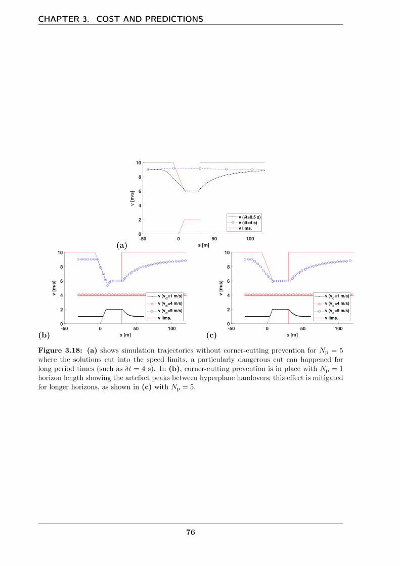
CHAPTER 3. COST AND PREDICTIONS
(a)-50 0 50 100
s [m]
0
2
4
6
8
10
v [
m/s
]
v ( t=0.5 s)
v ( t=4 s)
v lims.
(b)-50 0 50 100
s [m]
0
2
4
6
8
10
v [
m/s
]
v (vd=1 m/s)
v (vd=4 m/s)
v (vd=9 m/s)
v lims.
(c)-50 0 50 100
s [m]
0
2
4
6
8
10
v [
m/s
]
v (vd=1 m/s)
v (vd=4 m/s)
v (vd=9 m/s)
v lims.
Figure 3.18: (a) shows simulation trajectories without corner-cutting prevention for Np = 5where the solutions cut into the speed limits, a particularly dangerous cut can happened forlong period times (such as δt = 4 s). In (b), corner-cutting prevention is in place with Np = 1horizon length showing the artefact peaks between hyperplane handovers; this effect is mitigatedfor longer horizons, as shown in (c) with Np = 5.
76
4Cross-junction control and simulations
This chapter aims to expand the control framework to higher-scale simulations, increasingthe simulation length and the number of vehicles considered in the multi-agent models.The chosen test environment is a single simplistic cross junction, where complexity comesfrom the junction-passing arbitration between vehicles. After a brief introduction to thenumerical considerations for these simulations, the considered types of junction simula-tions and vehicle interactions will be discussed. Various control policies are introduced,formulated, and analysed in the context of junction examples; further investigation ismade into deadlock situations. The junction-passing completion approach is formulatedfor the so-called ‘box junctions’ using MIP techniques, which aim to solve deadlock issuesthat are common in busy intersections.
4.1 Problem statement
The number of agents (vehicles) within the system is N , moving on two junction arms.Let the west-to-east arm be referred to as arm1 and the south-to-north arm as arm2 withthe number of vehicles on them Narm1 and Narm2 , respectively. On Figure 4.1, the vehicleparameters are shown with the bounding box where the length parameter is L with anadded safety gap (vehicle length is L) and the width parameter is W , resulting in thepictured collision set C12.
The vehicles move on their respective junction arms and must remain safe while passingthrough the junction. As before, the vehicles are to optimise some measure of theirobjective and cooperate through centralised optimisation.
Cross junctions are inherently susceptible to gridlock or deadlock situations. In com-puter science, ‘deadlock’ situation is a state in which two or more processes have taskscompeting for a shared resource that can only be used by one at a time; the processesultimately block each other, resulting in neither gaining access to the resource or com-pleting their task in finite time without outside help. This state may be resolved through
77

CHAPTER 4. CROSS-JUNCTION CONTROL AND SIMULATIONS
Figure 4.1: (a) Schematic of a cross junction with orthogonal arms; (b) the constructed colli-sion set for a conflicting vehicle pair (the pictured scenario on (a) is indicated as the correspond-ing state position on (b)); (c) the rectangular bounding box design used with indicated vehicleparameters, including a constant safety zone in front of the vehicle—the foremost longitudinalposition of the bounding box serves as vehicle’s reference point.
additional or external action; without it, however, the system is paralysed indefinitely.Using this analogy, the vehicles moving through the junction are the tasks competingfor the shared resource. For example, a greedy driving policy makes a vehicle enter thejunction even when it is clear that it may not leave it for an unknown amount of time.Of course, in practice, traffic deadlocks and gridlocks are resolved in finite time due toeither outside help or the creative thinking of human drivers.
In comparison, Y-junction merging is structurally deadlock-free; a single greedy vehicleon one arm does not indefinitely obstruct traffic on the other arm, as it leaves the junction.
The box junction also has the benefit of being free of deadlocks, as it restricts entry.According to the UK Highway Code [77] for box junctions the indication is as follows:‘Box junctions have criss-cross yellow lines painted on the road (...) You MUST NOTenter the box until your exit road or lane is clear.’ [77, Rule 174], with some minorcondition on right turning vehicles.
4.2 Numerical considerations
The main simulation options, including the choice of cost function, modifications on dy-namics, and the simulation type are explained in the following sections.
78
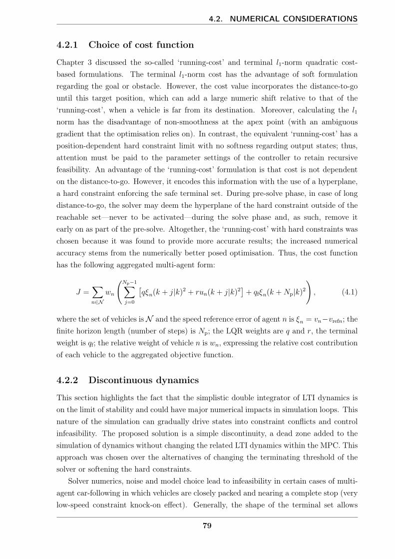
4.2. NUMERICAL CONSIDERATIONS
4.2.1 Choice of cost function
Chapter 3 discussed the so-called ‘running-cost’ and terminal l1-norm quadratic cost-based formulations. The terminal l1-norm cost has the advantage of soft formulationregarding the goal or obstacle. However, the cost value incorporates the distance-to-gountil this target position, which can add a large numeric shift relative to that of the‘running-cost’, when a vehicle is far from its destination. Moreover, calculating the l1norm has the disadvantage of non-smoothness at the apex point (with an ambiguousgradient that the optimisation relies on). In contrast, the equivalent ‘running-cost’ has aposition-dependent hard constraint limit with no softness regarding output states; thus,attention must be paid to the parameter settings of the controller to retain recursivefeasibility. An advantage of the ‘running-cost’ formulation is that cost is not dependenton the distance-to-go. However, it encodes this information with the use of a hyperplane,a hard constraint enforcing the safe terminal set. During pre-solve phase, in case of longdistance-to-go, the solver may deem the hyperplane of the hard constraint outside of thereachable set—never to be activated—during the solve phase and, as such, remove itearly on as part of the pre-solve. Altogether, the ‘running-cost’ with hard constraints waschosen because it was found to provide more accurate results; the increased numericalaccuracy stems from the numerically better posed optimisation. Thus, the cost functionhas the following aggregated multi-agent form:
J =∑n∈N
wn
(Np−1∑j=0
[qξn(k + j|k)2 + run(k + j|k)2
]+ qfξn(k +Np|k)2
), (4.1)
where the set of vehicles is N and the speed reference error of agent n is ξn = vn−vrefn; thefinite horizon length (number of steps) is Np; the LQR weights are q and r, the terminalweight is qf; the relative weight of vehicle n is wn, expressing the relative cost contributionof each vehicle to the aggregated objective function.
4.2.2 Discontinuous dynamics
This section highlights the fact that the simplistic double integrator of LTI dynamics ison the limit of stability and could have major numerical impacts in simulation loops. Thisnature of the simulation can gradually drive states into constraint conflicts and controlinfeasibility. The proposed solution is a simple discontinuity, a dead zone added to thesimulation of dynamics without changing the related LTI dynamics within the MPC. Thisapproach was chosen over the alternatives of changing the terminating threshold of thesolver or softening the hard constraints.
Solver numerics, noise and model choice lead to infeasibility in certain cases of multi-agent car-following in which vehicles are closely packed and nearing a complete stop (verylow-speed constraint knock-on effect). Generally, the shape of the terminal set allows
79

CHAPTER 4. CROSS-JUNCTION CONTROL AND SIMULATIONS
vehicles to asymptotically converge towards zero speed without ever reaching it in finitetime. This may also happen in a long queue of vehicles waiting for right of way, be it at ajunction or behind a road blockage in a deadlock situation. After a certain amount of timehas elapsed, the optimisation may encounter infeasibility, which seemingly contradicts thetheory that has been formulated so far. However, this issue can be traced back to thetype of idealised kinematics rule described by the double integrator. Matrix A in (2.8) hasλ = 1 double eigenvalues placed; with the nature of integrators come the accumulation ofnegligible numerical noise and imperfections over a long period.
In the case of asymptotically converging speed, the control input (acceleration) isnever truly zero while the inherent numerical noise is present. This noise is relativelysmall and originates from complex solving procedures and finite precision arithmetic er-rors. For vehicles in motion, with higher-than-negligible speed, the controller has enoughroom to accommodate the small imperfections—this numerical noise. In contrast, tightlypacked vehicle queues have few feasible state choices available because the hard con-straints, defined for each vehicle, move closer together, leaving less and less space toaccommodate the integrated noise in each control step. This effect eventually causes thehard constraints to be violated and to exceed the solver infeasibility tolerance threshold.
In order to solve this infeasibility issue, the origins of the numerical noise must bewell understood. One source of the noise is the termination of the solver algorithm itself.In convex problems, the solver provides the optimal solution and the certificate of globaloptimality (zero duality gap). In practice, however, this solution is arbitrary within thevicinity of the absolute optimum, where the terminating conditions of the algorithms aresatisfied. Note the similar case of termination for the integer decisions in the MIP problem,where the algorithm may terminate early at the point at which it satisfies all thresholdconditions. This can be advantageous in the branch-and-bound algorithm, trading MIPoptimality gap (slight sub-optimality) for higher computation speed. In other words, thismay result in two mathematically and numerically ideal problem yielding different non-unique results, where the solver has the full discretion to select which answer it returnsdespite any of them being valid.
Tightening the default threshold criteria of the solver—which, to a point, results inmore accurate solutions—is a naïve approach, as the improvement is disproportional. Theapproach increases the number of iterations necessary to reach the termination conditionsand the solution. Of course, this has a negative effect on the computation time of theoptimisation. However, changing threshold settings cannot remove the inherent digitalnoise from the floating-point representation; in practice, it defines a natural lower limitof accuracy and a minimum value of threshold parameters. As expected, higher accuracyincreased the queuing time of vehicles before the optimisation inside the controller reachedthe infeasibility message—verifying that the integrated noise is smaller but ultimately nota solution to the issue.
80
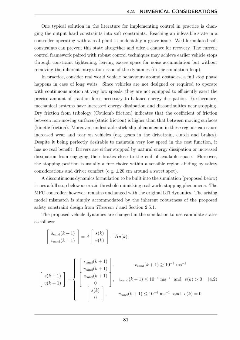
4.2. NUMERICAL CONSIDERATIONS
One typical solution in the literature for implementing control in practice is chan-ging the output hard constraints into soft constraints. Reaching an infeasible state in acontroller operating with a real plant is undeniably a grave issue. Well-formulated softconstraints can prevent this state altogether and offer a chance for recovery. The currentcontrol framework paired with robust control techniques may achieve earlier vehicle stopsthrough constraint tightening, leaving excess space for noise accumulation but withoutremoving the inherent integration issue of the dynamics (in the simulation loop).
In practice, consider real world vehicle behaviours around obstacles, a full stop phasehappens in case of long waits. Since vehicles are not designed or required to operatewith continuous motion at very low speeds, they are not equipped to efficiently exert theprecise amount of traction force necessary to balance energy dissipation. Furthermore,mechanical systems have increased energy dissipation and discontinuities near stopping.Dry friction from tribology (Coulomb friction) indicates that the coefficient of frictionbetween non-moving surfaces (static friction) is higher than that between moving surfaces(kinetic friction). Moreover, undesirable stick-slip phenomenon in these regions can causeincreased wear and tear on vehicles (e.g. gears in the drivetrain, clutch and brakes).Despite it being perfectly desirable to maintain very low speed in the cost function, ithas no real benefit. Drivers are either stopped by natural energy dissipation or increaseddissipation from engaging their brakes close to the end of available space. Moreover,the stopping position is usually a free choice within a sensible region abiding by safetyconsiderations and driver comfort (e.g. ±20 cm around a sweet spot).
A discontinuous dynamics formulation to be built into the simulation (proposed below)issues a full stop below a certain threshold mimicking real-world stopping phenomena. TheMPC controller, however, remains unchanged with the original LTI dynamics. The arisingmodel mismatch is simply accommodated by the inherent robustness of the proposedsafety constraint design from Theorem 1 and Section 2.5.1.
The proposed vehicle dynamics are changed in the simulation to use candidate statesas follows:[
scand(k + 1)
vcand(k + 1)
]= A
[s(k)
v(k)
]+Bu(k),
[s(k + 1)
v(k + 1)
]=
[scand(k + 1)
vcand(k + 1)
], vcand(k + 1) ≥ 10−4 ms−1[
scand(k + 1)
0
], vcand(k + 1) ≤ 10−4 ms−1 and v(k) > 0[
s(k)
0
], vcand(k + 1) ≤ 10−4 ms−1 and v(k) = 0.
(4.2)
81
CHAPTER 4. CROSS-JUNCTION CONTROL AND SIMULATIONS
The threshold setting of v ≥ 10−4 ms−1 by assuming a headway time of 2 s correspondsto the earliest stop of 0.2 mm away from the obstacle point. This, from engineeringperspective, is negligible change; provides appropriate margins for a numerically stable,(static) long-queue simulation.
4.3 Simulation types
The simulated scenarios are within a spatially restricted region of the traffic networkdefined by spatial and temporal boundaries as well as initial conditions that require as-sumptions about the outside (not simulated) traffic states. This work does not aim tocreate a perfect replica of real-world traffic; rather, it aims to use the simulations as ameans to challenge the proposed control through the choice of boundary assumptions.Three simulation types are introduced in this section to conduct analyses on them. Thecases are able to develop continuous traffic, settling to steady-state or periodic trafficflows; moreover, generating vehicle inflows from sampled distributions allow long-termsimulations to be run and later obtain broader statistical measures.
This chapter discusses a single road crossing and junction area, providing a mixtureof car-following and crossing-order decisions. An appealing type of simulation involvesfixing the number of vehicles to yield constant average traffic densities [75]. There isa given number of vehicles travelling on each junction arm; when a vehicle leaves itssimulated road at the outlet, it reappears at the inlet. The advantage of this simulationis the constant complexity of the control, as the fixed number of vehicles yields a fixednumber of states and decision variables. In traffic simulations, reintroduction of vehiclesmimics the self-similar junction scenarios that arise in urban traffic networks. An urbandistrict with largely similar junctions (e.g. a grid) can be simulated via a single cell thatis expected to develop realistic inlet and outlet traffic measures. In Section 4.3.2, an8-loop-shaped simulation type is shown with similarly fixed average traffic densities; thissimulation type is later used to analyse average traffic measures, traffic flows and densitieswith fundamental diagrams [75] as well as further investigate deadlocks stemming fromhigh traffic density and control-policy behaviour.
Finally, the junction arm inlet flows are randomly and independently generated inthe third simulation type following a general truncated exponential distribution fromAppendix B. The inlets in this case produce random vehicle arrivals with no memoryeffect of how vehicles leave the simulated cell. This results in the negative effect of varyingnumber of simulated vehicles and the knock-on effect on complexity yet provides randomand still intensive interactions for junction arbitration to challenge a control policy.
82

4.3. SIMULATION TYPES
Figure 4.2: Two-arm cross-junction simulation type with road/lane-wise vehicle introductionfrom the buffer region. This simulation type keeps the number of vehicles, and in turn, thetraffic density in the simulation constant. The junction arms each have equal dc-characteristicarm length.
4.3.1 Fixed number of vehicles—O-loops
First, consider the junction area where a vehicle reaching the end of its road wouldenter a buffer region. From this buffer region, at each simulation time step, the vehicle is‘reintroduced’ as a new vehicle at the beginning of the same road with the same or changedvehicle properties. Such a mechanism is shown in Figure 4.2, where the characteristic armlength is dc. The buffer area is used to hold vehicles while reintroducing them is unsafe (i.e.the car-following constraint would yield a trivial conflict when the previously reintroducedcar has not physically cleared the area yet). Moreover, vehicles have the opportunity tochange their states or parameters while reappearing (e.g. changing desired speed).
4.3.2 Fixed number of vehicles—8-loops
When the outlet of arm1 is connected to the inlet of arm2 (and vice-versa), an ‘8-loop’ isformed (see Figure 4.3, which shows symmetric loops with the characteristic arm lengthdc). In this case, the last vehicle on arm1 is simply following the first vehicle on arm2, andvice-versa, removing the need for a buffer region and allowing for seamless vehicle flow.This simulation type can be used to analyse emerging tendencies of long-term simulationsin a closed system, for example, steady-state modes, average measures, and stationarysolutions.
83
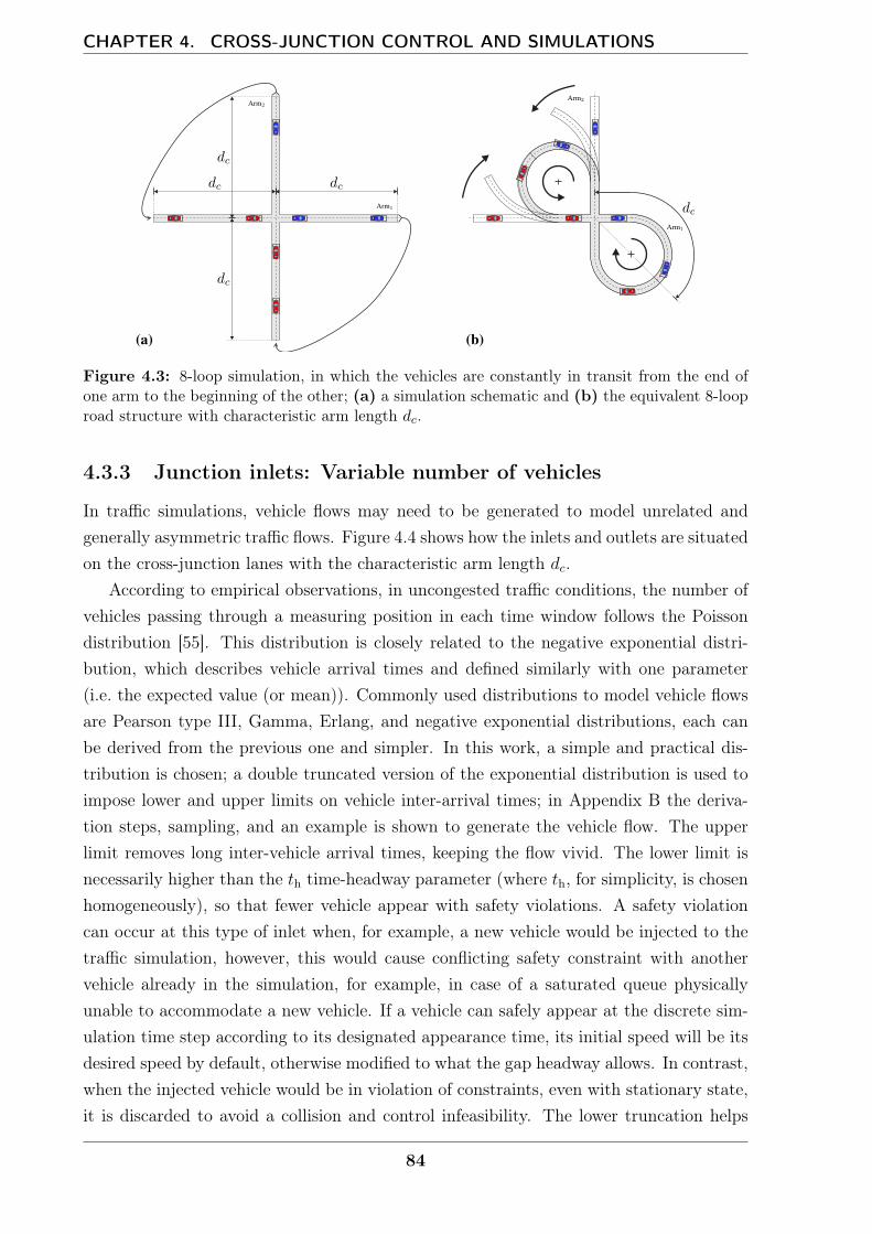
CHAPTER 4. CROSS-JUNCTION CONTROL AND SIMULATIONS
Figure 4.3: 8-loop simulation, in which the vehicles are constantly in transit from the end ofone arm to the beginning of the other; (a) a simulation schematic and (b) the equivalent 8-looproad structure with characteristic arm length dc.
4.3.3 Junction inlets: Variable number of vehicles
In traffic simulations, vehicle flows may need to be generated to model unrelated andgenerally asymmetric traffic flows. Figure 4.4 shows how the inlets and outlets are situatedon the cross-junction lanes with the characteristic arm length dc.
According to empirical observations, in uncongested traffic conditions, the number ofvehicles passing through a measuring position in each time window follows the Poissondistribution [55]. This distribution is closely related to the negative exponential distri-bution, which describes vehicle arrival times and defined similarly with one parameter(i.e. the expected value (or mean)). Commonly used distributions to model vehicle flowsare Pearson type III, Gamma, Erlang, and negative exponential distributions, each canbe derived from the previous one and simpler. In this work, a simple and practical dis-tribution is chosen; a double truncated version of the exponential distribution is used toimpose lower and upper limits on vehicle inter-arrival times; in Appendix B the deriva-tion steps, sampling, and an example is shown to generate the vehicle flow. The upperlimit removes long inter-vehicle arrival times, keeping the flow vivid. The lower limit isnecessarily higher than the th time-headway parameter (where th, for simplicity, is chosenhomogeneously), so that fewer vehicle appear with safety violations. A safety violationcan occur at this type of inlet when, for example, a new vehicle would be injected to thetraffic simulation, however, this would cause conflicting safety constraint with anothervehicle already in the simulation, for example, in case of a saturated queue physicallyunable to accommodate a new vehicle. If a vehicle can safely appear at the discrete sim-ulation time step according to its designated appearance time, its initial speed will be itsdesired speed by default, otherwise modified to what the gap headway allows. In contrast,when the injected vehicle would be in violation of constraints, even with stationary state,it is discarded to avoid a collision and control infeasibility. The lower truncation helps
84
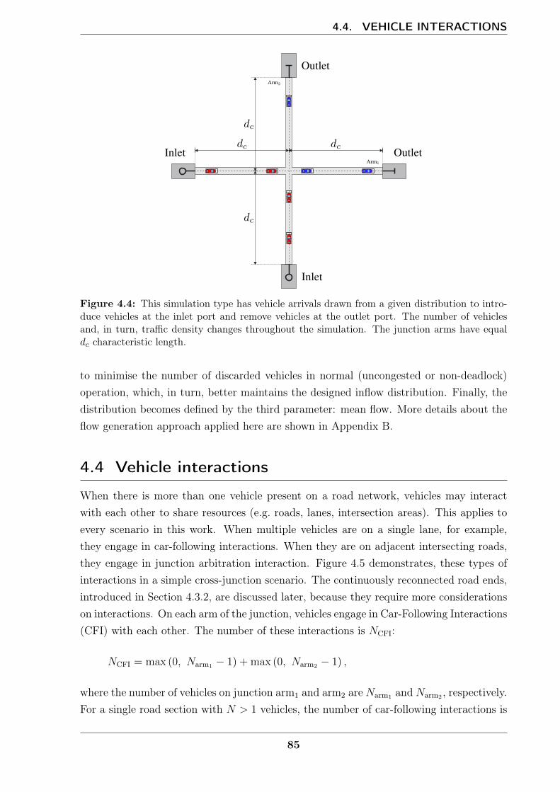
4.4. VEHICLE INTERACTIONS
Figure 4.4: This simulation type has vehicle arrivals drawn from a given distribution to intro-duce vehicles at the inlet port and remove vehicles at the outlet port. The number of vehiclesand, in turn, traffic density changes throughout the simulation. The junction arms have equaldc characteristic length.
to minimise the number of discarded vehicles in normal (uncongested or non-deadlock)operation, which, in turn, better maintains the designed inflow distribution. Finally, thedistribution becomes defined by the third parameter: mean flow. More details about theflow generation approach applied here are shown in Appendix B.
4.4 Vehicle interactions
When there is more than one vehicle present on a road network, vehicles may interactwith each other to share resources (e.g. roads, lanes, intersection areas). This applies toevery scenario in this work. When multiple vehicles are on a single lane, for example,they engage in car-following interactions. When they are on adjacent intersecting roads,they engage in junction arbitration interaction. Figure 4.5 demonstrates, these types ofinteractions in a simple cross-junction scenario. The continuously reconnected road ends,introduced in Section 4.3.2, are discussed later, because they require more considerationson interactions. On each arm of the junction, vehicles engage in Car-Following Interactions(CFI) with each other. The number of these interactions is NCFI:
NCFI = max (0, Narm1 − 1) + max (0, Narm2 − 1) ,
where the number of vehicles on junction arm1 and arm2 are Narm1 and Narm2 , respectively.For a single road section with N > 1 vehicles, the number of car-following interactions is
85

CHAPTER 4. CROSS-JUNCTION CONTROL AND SIMULATIONS
Figure 4.5: Vehicle interactions in a simple two-arm crossing scenario.
N − 1; N ≡ 1 imposes zero car-following pairs.Car-following constraints were introduced in Section 2.3.4; recall that:
sp (k + j|k) + thvp (k + j|k) ≤ sq (k + j + 1|k)− Lq, (4.3)
where the leader vehicle index is q with safety padded length Lq and the follower vehicleindex is p with the time headway th as an arbitrary choice of the follower with the lowerbound depending on the follower vehicle capabilities; j = 0, 1, . . . Np. These constraintsmust be added ∀ (p, q) ∈ NCFI vehicle pairs, where the set of all car-following interactionsis NCFI composed of the ordered follower–leader subsets (p, q), defined over vehicle indices.
Furthermore, similarly to that in the merging junction, the arbitration-related Junc-tion Crossing Interaction (JCI) in cross junctions can be readily determined, as shownin Figure 4.1. Following this logic, all pairs of vehicles p, q with JCI between themare collected as subsets of the NJCI set. In a simplistic approach, an interaction must begenerated for each vehicle on one arm with each vehicle on the other arm (since Cpq 6= ∅).By repeating this process, the overall number of pairwise junction collision sets is:
NJCI = Narm1 Narm2 .
As shown in Figure 4.5, the junction arbitration corresponding to the interaction of eachjunction collision set or decision-making process may be either active (waiting for decision)or decided (arbitrated). This property comes from the evolution of states (e.g. when avehicle has cleared the junction area, the ordering decision can no longer be changed, sincethe vehicles are not allowed to move backwards). From this consideration, NJCI ⊆ NJCI
and NJCI ≤ NJCI, where the set of active junction arbitration interactions is NJCI and thenumber of vehicle pairs is NJCI, where neither p nor q has cleared the junction yet. Note
86
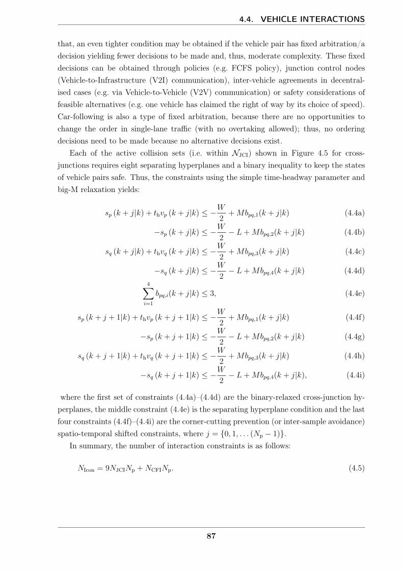
4.4. VEHICLE INTERACTIONS
that, an even tighter condition may be obtained if the vehicle pair has fixed arbitration/adecision yielding fewer decisions to be made and, thus, moderate complexity. These fixeddecisions can be obtained through policies (e.g. FCFS policy), junction control nodes(Vehicle-to-Infrastructure (V2I) communication), inter-vehicle agreements in decentral-ised cases (e.g. via Vehicle-to-Vehicle (V2V) communication) or safety considerations offeasible alternatives (e.g. one vehicle has claimed the right of way by its choice of speed).Car-following is also a type of fixed arbitration, because there are no opportunities tochange the order in single-lane traffic (with no overtaking allowed); thus, no orderingdecisions need to be made because no alternative decisions exist.
Each of the active collision sets (i.e. within NJCI) shown in Figure 4.5 for cross-junctions requires eight separating hyperplanes and a binary inequality to keep the statesof vehicle pairs safe. Thus, the constraints using the simple time-headway parameter andbig-M relaxation yields:
sp (k + j|k) + thvp (k + j|k) ≤ −W2
+Mbpq,1(k + j|k) (4.4a)
−sp (k + j|k) ≤ −W2− L+Mbpq,2(k + j|k) (4.4b)
sq (k + j|k) + thvq (k + j|k) ≤ −W2
+Mbpq,3(k + j|k) (4.4c)
−sq (k + j|k) ≤ −W2− L+Mbpq,4(k + j|k) (4.4d)
4∑i=1
bpq,i(k + j|k) ≤ 3, (4.4e)
sp (k + j + 1|k) + thvp (k + j + 1|k) ≤ −W2
+Mbpq,1(k + j|k) (4.4f)
−sp (k + j + 1|k) ≤ −W2− L+Mbpq,2(k + j|k) (4.4g)
sq (k + j + 1|k) + thvq (k + j + 1|k) ≤ −W2
+Mbpq,3(k + j|k) (4.4h)
−sq (k + j + 1|k) ≤ −W2− L+Mbpq,4(k + j|k), (4.4i)
where the first set of constraints (4.4a)–(4.4d) are the binary-relaxed cross-junction hy-perplanes, the middle constraint (4.4e) is the separating hyperplane condition and the lastfour constraints (4.4f)–(4.4i) are the corner-cutting prevention (or inter-sample avoidance)spatio-temporal shifted constraints, where j = 0, 1, . . . (Np − 1).
In summary, the number of interaction constraints is as follows:
NIcon = 9NJCINp +NCFINp. (4.5)
87
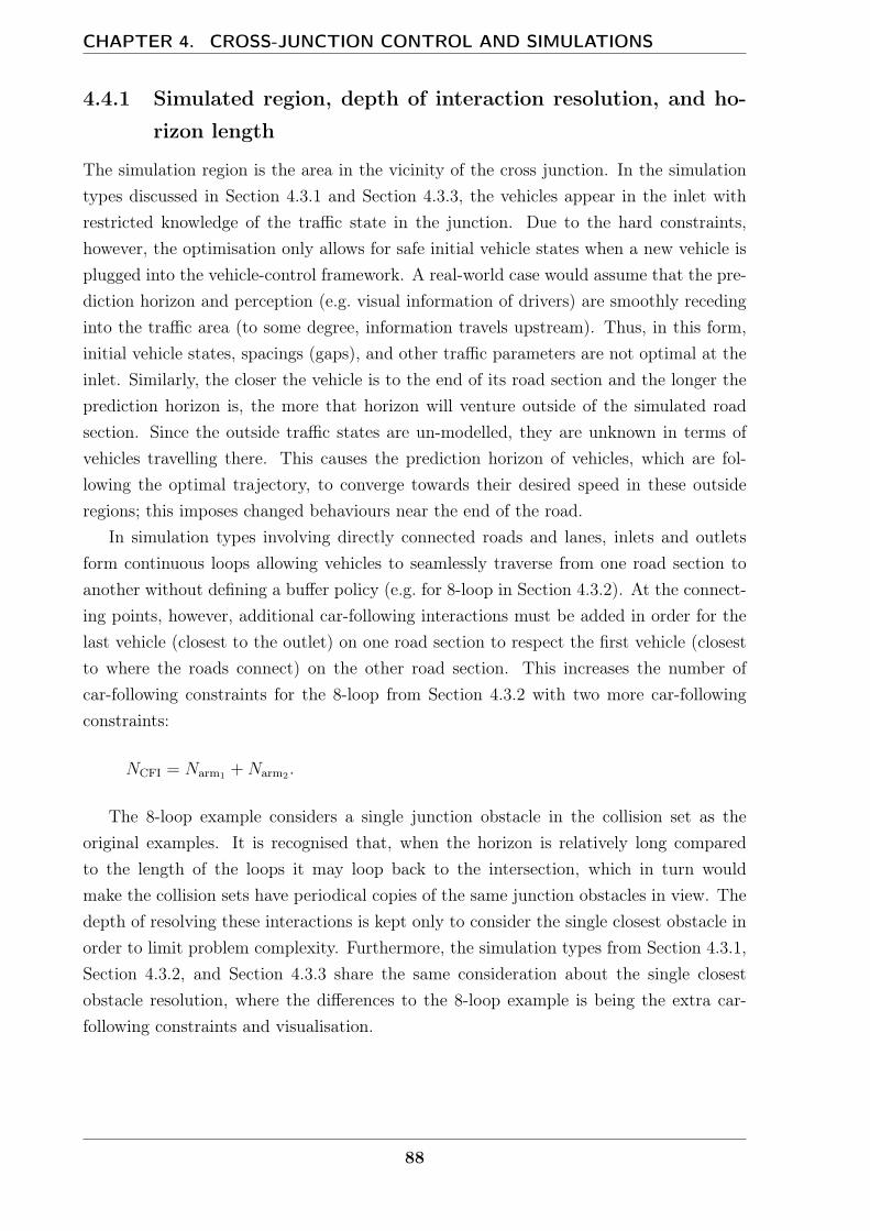
CHAPTER 4. CROSS-JUNCTION CONTROL AND SIMULATIONS
4.4.1 Simulated region, depth of interaction resolution, and ho-
rizon length
The simulation region is the area in the vicinity of the cross junction. In the simulationtypes discussed in Section 4.3.1 and Section 4.3.3, the vehicles appear in the inlet withrestricted knowledge of the traffic state in the junction. Due to the hard constraints,however, the optimisation only allows for safe initial vehicle states when a new vehicle isplugged into the vehicle-control framework. A real-world case would assume that the pre-diction horizon and perception (e.g. visual information of drivers) are smoothly recedinginto the traffic area (to some degree, information travels upstream). Thus, in this form,initial vehicle states, spacings (gaps), and other traffic parameters are not optimal at theinlet. Similarly, the closer the vehicle is to the end of its road section and the longer theprediction horizon is, the more that horizon will venture outside of the simulated roadsection. Since the outside traffic states are un-modelled, they are unknown in terms ofvehicles travelling there. This causes the prediction horizon of vehicles, which are fol-lowing the optimal trajectory, to converge towards their desired speed in these outsideregions; this imposes changed behaviours near the end of the road.
In simulation types involving directly connected roads and lanes, inlets and outletsform continuous loops allowing vehicles to seamlessly traverse from one road section toanother without defining a buffer policy (e.g. for 8-loop in Section 4.3.2). At the connect-ing points, however, additional car-following interactions must be added in order for thelast vehicle (closest to the outlet) on one road section to respect the first vehicle (closestto where the roads connect) on the other road section. This increases the number ofcar-following constraints for the 8-loop from Section 4.3.2 with two more car-followingconstraints:
NCFI = Narm1 +Narm2 .
The 8-loop example considers a single junction obstacle in the collision set as theoriginal examples. It is recognised that, when the horizon is relatively long comparedto the length of the loops it may loop back to the intersection, which in turn wouldmake the collision sets have periodical copies of the same junction obstacles in view. Thedepth of resolving these interactions is kept only to consider the single closest obstacle inorder to limit problem complexity. Furthermore, the simulation types from Section 4.3.1,Section 4.3.2, and Section 4.3.3 share the same consideration about the single closestobstacle resolution, where the differences to the 8-loop example is being the extra car-following constraints and visualisation.
88
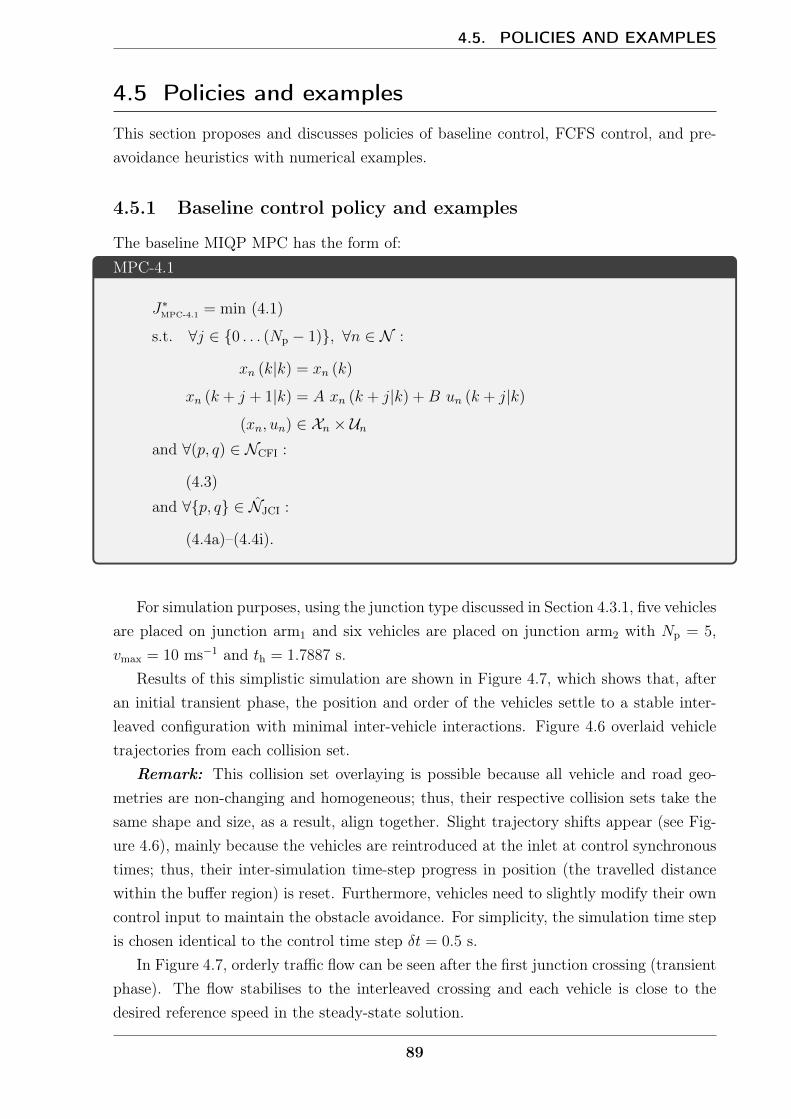
4.5. POLICIES AND EXAMPLES
4.5 Policies and examples
This section proposes and discusses policies of baseline control, FCFS control, and pre-avoidance heuristics with numerical examples.
4.5.1 Baseline control policy and examples
The baseline MIQP MPC has the form of:MPC-4.1
J∗MPC-4.1 = min (4.1)
s.t. ∀j ∈ 0 . . . (Np − 1), ∀n ∈ N :
xn (k|k) = xn (k)
xn (k + j + 1|k) = A xn (k + j|k) +B un (k + j|k)
(xn, un) ∈ Xn × Unand ∀(p, q) ∈ NCFI :
(4.3)
and ∀p, q ∈ NJCI :
(4.4a)–(4.4i).
For simulation purposes, using the junction type discussed in Section 4.3.1, five vehiclesare placed on junction arm1 and six vehicles are placed on junction arm2 with Np = 5,vmax = 10 ms−1 and th = 1.7887 s.
Results of this simplistic simulation are shown in Figure 4.7, which shows that, afteran initial transient phase, the position and order of the vehicles settle to a stable inter-leaved configuration with minimal inter-vehicle interactions. Figure 4.6 overlaid vehicletrajectories from each collision set.
Remark: This collision set overlaying is possible because all vehicle and road geo-metries are non-changing and homogeneous; thus, their respective collision sets take thesame shape and size, as a result, align together. Slight trajectory shifts appear (see Fig-ure 4.6), mainly because the vehicles are reintroduced at the inlet at control synchronoustimes; thus, their inter-simulation time-step progress in position (the travelled distancewithin the buffer region) is reset. Furthermore, vehicles need to slightly modify their owncontrol input to maintain the obstacle avoidance. For simplicity, the simulation time stepis chosen identical to the control time step δt = 0.5 s.
In Figure 4.7, orderly traffic flow can be seen after the first junction crossing (transientphase). The flow stabilises to the interleaved crossing and each vehicle is close to thedesired reference speed in the steady-state solution.
89
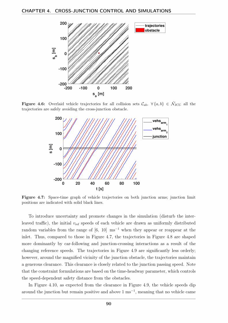
CHAPTER 4. CROSS-JUNCTION CONTROL AND SIMULATIONS
-200 -100 0 100 200
sa [m]
-200
-100
0
100
200
sb [
m]
trajectories
obstacle
Figure 4.6: Overlaid vehicle trajectories for all collision sets Cab, ∀ a, b ∈ NJCI; all thetrajectories are safely avoiding the cross-junction obstacle.
0 20 40 60 80 100
t [s]
-200
-100
0
100
200
s [
m]
vehsarm
1
vehsarm
2
junction
Figure 4.7: Space-time graph of vehicle trajectories on both junction arms; junction limitpositions are indicated with solid black lines.
To introduce uncertainty and promote changes in the simulation (disturb the inter-leaved traffic), the initial vref speeds of each vehicle are drawn as uniformly distributedrandom variables from the range of [6, 10] ms−1 when they appear or reappear at theinlet. Thus, compared to those in Figure 4.7, the trajectories in Figure 4.8 are shapedmore dominantly by car-following and junction-crossing interactions as a result of thechanging reference speeds. The trajectories in Figure 4.9 are significantly less orderly;however, around the magnified vicinity of the junction obstacle, the trajectories maintaina generous clearance. This clearance is closely related to the junction passing speed. Notethat the constraint formulations are based on the time-headway parameter, which controlsthe speed-dependent safety distance from the obstacles.
In Figure 4.10, as expected from the clearance in Figure 4.9, the vehicle speeds diparound the junction but remain positive and above 1 ms−1, meaning that no vehicle came
90

4.5. POLICIES AND EXAMPLES
0 50 100 150 200 250
t [s]
-200
-100
0
100
200
s [
m]
vehsarm
1
vehsarm
2
junction
Figure 4.8: Space-time graph of vehicle trajectories on both junction arms; junction limit posi-tions are indicated with solid black lines; vehicle reference speeds chosen in the range [6, 10] ms−1.
(a)-200 -100 0 100 200
sa [m]
-200
-100
0
100
200
sb [
m]
(b)-20 -10 0 10 20
sa [m]
-20
-10
0
10
20s
b [
m]
trajectories
obstacle
Figure 4.9: Vehicle trajectories overlaid and shown for all collision sets with the junctionobstacle indicated in (a) and magnified in (b).
to a full stop.Two particular artefacts show the simulation issues of inlets and outlets, visible in
Figure 4.10. Starting with the outlet artefact, the problem stems from the predictivenature of the control and the vehicles vanishing at the outlet. First, it must be understoodthat, as the reference speeds are random variables, the vehicles with higher referencespeeds are likely to catch up with the vehicle travelling ahead in the same lane at a slowerspeed. After the faster vehicle catches up to the slower one, they settle on a mutuallybeneficial speed regulated by their car-following interaction and the related constraints.Once at the outlet, the slower vehicle is removed from the simulation, meaning that thevehicle behind it travelling slower than its desired speed can accelerate, since the car-following interaction with the slow leader vehicle is also removed. This speed-up artefactcan be witnessed on some of the trajectories closest to the outlet.
The inlet artefact is also observed which, similarly, reflects the missing informationof the traffic outside the simulation. Generally, when a control is turned on in a system,
91
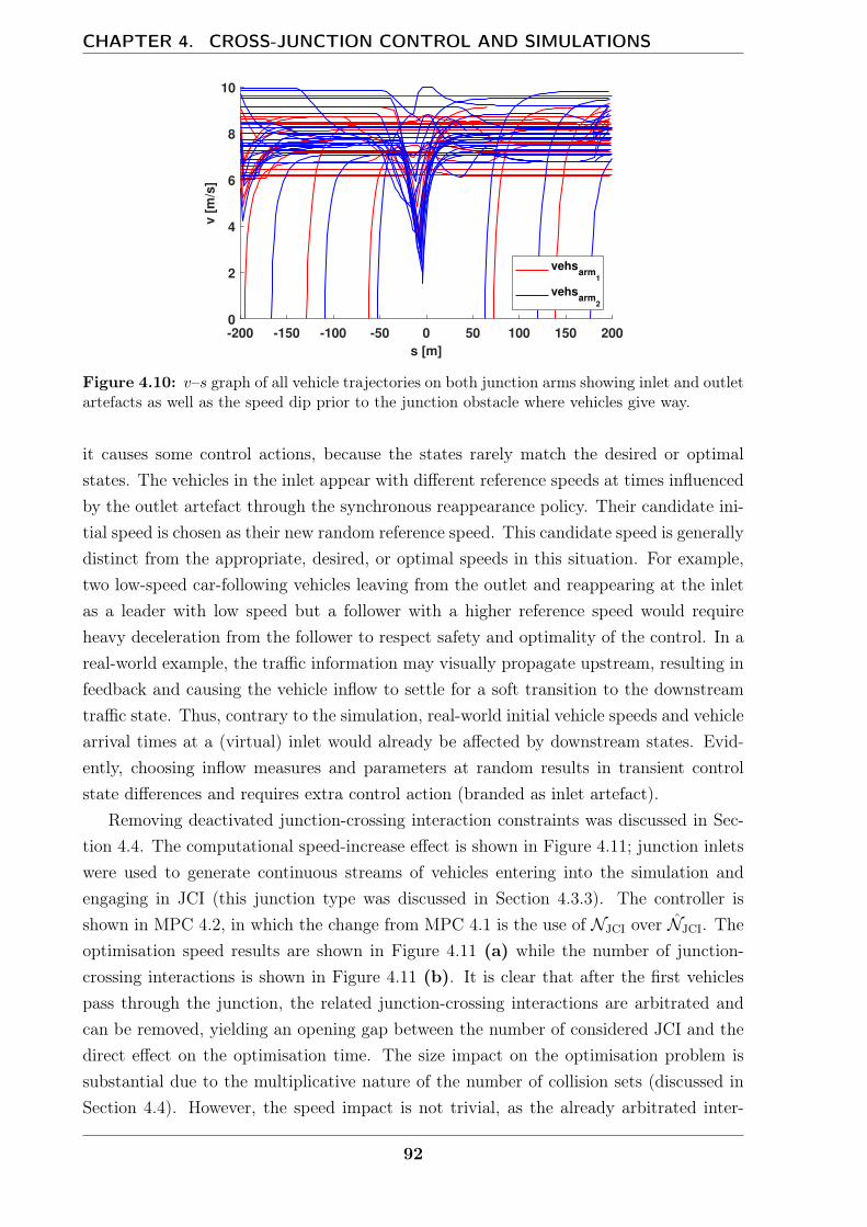
CHAPTER 4. CROSS-JUNCTION CONTROL AND SIMULATIONS
-200 -150 -100 -50 0 50 100 150 200
s [m]
0
2
4
6
8
10
v [
m/s
]
vehsarm
1
vehsarm
2
Figure 4.10: v–s graph of all vehicle trajectories on both junction arms showing inlet and outletartefacts as well as the speed dip prior to the junction obstacle where vehicles give way.
it causes some control actions, because the states rarely match the desired or optimalstates. The vehicles in the inlet appear with different reference speeds at times influencedby the outlet artefact through the synchronous reappearance policy. Their candidate ini-tial speed is chosen as their new random reference speed. This candidate speed is generallydistinct from the appropriate, desired, or optimal speeds in this situation. For example,two low-speed car-following vehicles leaving from the outlet and reappearing at the inletas a leader with low speed but a follower with a higher reference speed would requireheavy deceleration from the follower to respect safety and optimality of the control. In areal-world example, the traffic information may visually propagate upstream, resulting infeedback and causing the vehicle inflow to settle for a soft transition to the downstreamtraffic state. Thus, contrary to the simulation, real-world initial vehicle speeds and vehiclearrival times at a (virtual) inlet would already be affected by downstream states. Evid-ently, choosing inflow measures and parameters at random results in transient controlstate differences and requires extra control action (branded as inlet artefact).
Removing deactivated junction-crossing interaction constraints was discussed in Sec-tion 4.4. The computational speed-increase effect is shown in Figure 4.11; junction inletswere used to generate continuous streams of vehicles entering into the simulation andengaging in JCI (this junction type was discussed in Section 4.3.3). The controller isshown in MPC 4.2, in which the change from MPC 4.1 is the use of NJCI over NJCI. Theoptimisation speed results are shown in Figure 4.11 (a) while the number of junction-crossing interactions is shown in Figure 4.11 (b). It is clear that after the first vehiclespass through the junction, the related junction-crossing interactions are arbitrated andcan be removed, yielding an opening gap between the number of considered JCI and thedirect effect on the optimisation time. The size impact on the optimisation problem issubstantial due to the multiplicative nature of the number of collision sets (discussed inSection 4.4). However, the speed impact is not trivial, as the already arbitrated inter-
92

4.5. POLICIES AND EXAMPLES
actions should yield low-complexity decision in the branch-and-bound method since thebinaries are indirectly fixed by the vehicle states. This simple pre-processing results infaster calculation, exemplified by an average 33% decrease in computational time for thissimulation. The total simulation time with all JCI included was 5.8 s for 500 controliterations (and, with only the active JCI, 3.86 s).
MPC-4.2
J∗MPC-4.2 = min (4.1)
s.t. ∀j ∈ 0 . . . (Np − 1), ∀n ∈ N :
xn (k|k) = xn (k)
xn (k + j + 1|k) = A xn (k + j|k) +B un (k + j|k)
(xn, un) ∈ Xn × Unand ∀(p, q) ∈ NCFI :
(4.3)
and ∀p, q ∈ NJCI :
(4.4a)–(4.4i)
Remark: The optimisation time was measured with the reasonably smooth Matlabtic-toc timer function because the built-in Gurobi timer was found to have crude discretesteps in the range of interest (milliseconds); it often returned 0 s for fast optimisations,which holds little value in a comparison. Additionally, the discontinuous and discretesteps of the Gurobi timer were found to bias statistical results compared to the closer-to-real-time high-resolution measurements from Matlab. In comparison, the Matlab tic-toctimer function, which was chosen for its consistency, incorporates an extra overhead ofthe solver interface time as well as other factors from the task scheduling of the operatingsystem, resulting, in average, readings slightly higher than the raw optimisation time.The two simulation results (with MPC 4.1 and MPC 4.2) yield identical vehicle states, asexpected, and, thus, are deemed to be a fair comparison.
93
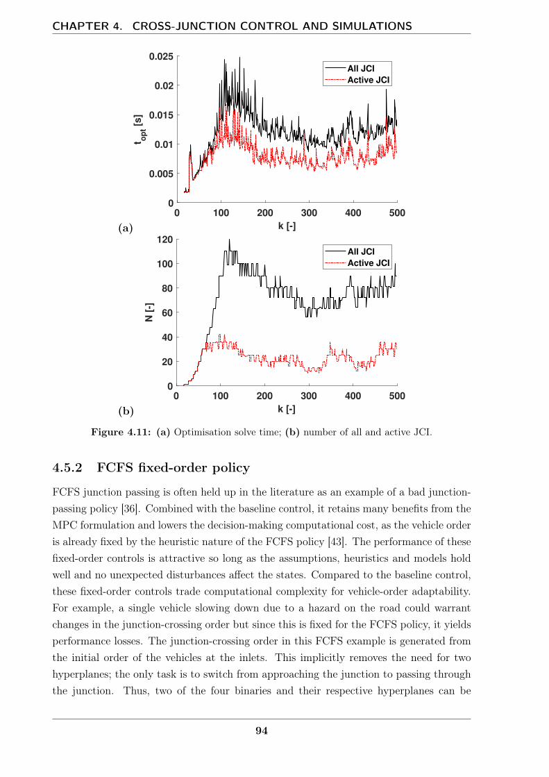
CHAPTER 4. CROSS-JUNCTION CONTROL AND SIMULATIONS
(a)0 100 200 300 400 500
k [-]
0
0.005
0.01
0.015
0.02
0.025
t op
t [s
]
All JCI
Active JCI
(b)0 100 200 300 400 500
k [-]
0
20
40
60
80
100
120
N [
-]
All JCI
Active JCI
Figure 4.11: (a) Optimisation solve time; (b) number of all and active JCI.
4.5.2 FCFS fixed-order policy
FCFS junction passing is often held up in the literature as an example of a bad junction-passing policy [36]. Combined with the baseline control, it retains many benefits from theMPC formulation and lowers the decision-making computational cost, as the vehicle orderis already fixed by the heuristic nature of the FCFS policy [43]. The performance of thesefixed-order controls is attractive so long as the assumptions, heuristics and models holdwell and no unexpected disturbances affect the states. Compared to the baseline control,these fixed-order controls trade computational complexity for vehicle-order adaptability.For example, a single vehicle slowing down due to a hazard on the road could warrantchanges in the junction-crossing order but since this is fixed for the FCFS policy, it yieldsperformance losses. The junction-crossing order in this FCFS example is generated fromthe initial order of the vehicles at the inlets. This implicitly removes the need for twohyperplanes; the only task is to switch from approaching the junction to passing throughthe junction. Thus, two of the four binaries and their respective hyperplanes can be
94
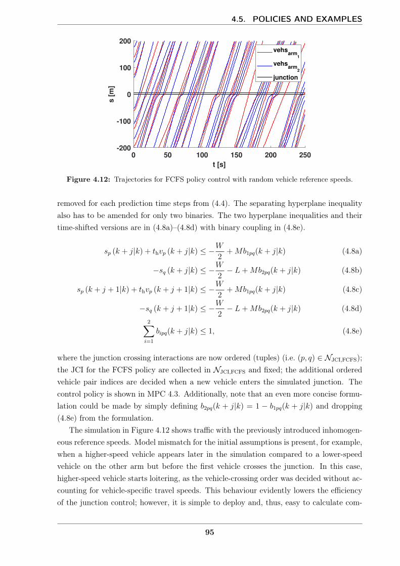
4.5. POLICIES AND EXAMPLES
0 50 100 150 200 250
t [s]
-200
-100
0
100
200
s [
m]
vehsarm
1
vehsarm
2
junction
Figure 4.12: Trajectories for FCFS policy control with random vehicle reference speeds.
removed for each prediction time steps from (4.4). The separating hyperplane inequalityalso has to be amended for only two binaries. The two hyperplane inequalities and theirtime-shifted versions are in (4.8a)–(4.8d) with binary coupling in (4.8e).
sp (k + j|k) + thvp (k + j|k) ≤ −W2
+Mb1pq(k + j|k) (4.8a)
−sq (k + j|k) ≤ −W2− L+Mb2pq(k + j|k) (4.8b)
sp (k + j + 1|k) + thvp (k + j + 1|k) ≤ −W2
+Mb1pq(k + j|k) (4.8c)
−sq (k + j + 1|k) ≤ −W2− L+Mb2pq(k + j|k) (4.8d)
2∑i=1
bipq(k + j|k) ≤ 1, (4.8e)
where the junction crossing interactions are now ordered (tuples) (i.e. (p, q) ∈ NJCI,FCFS);the JCI for the FCFS policy are collected in NJCI,FCFS and fixed; the additional orderedvehicle pair indices are decided when a new vehicle enters the simulated junction. Thecontrol policy is shown in MPC 4.3. Additionally, note that an even more concise formu-lation could be made by simply defining b2pq(k + j|k) = 1 − b1pq(k + j|k) and dropping(4.8e) from the formulation.
The simulation in Figure 4.12 shows traffic with the previously introduced inhomogen-eous reference speeds. Model mismatch for the initial assumptions is present, for example,when a higher-speed vehicle appears later in the simulation compared to a lower-speedvehicle on the other arm but before the first vehicle crosses the junction. In this case,higher-speed vehicle starts loitering, as the vehicle-crossing order was decided without ac-counting for vehicle-specific travel speeds. This behaviour evidently lowers the efficiencyof the junction control; however, it is simple to deploy and, thus, easy to calculate com-
95

CHAPTER 4. CROSS-JUNCTION CONTROL AND SIMULATIONS
(a)-200 -100 0 100 200
sa [m]
-200
-100
0
100
200
sb [
m]
(b)-20 -10 0 10 20
sa [m]
-20
-10
0
10
20
sb [
m]
trajectories
obstacle
Figure 4.13: Vehicle trajectories overlaid for FCFS control and shown for all collision sets withthe junction obstacle indicated in (a) and magnified in (b)
-200 -150 -100 -50 0 50 100 150 200
s [m]
0
2
4
6
8
10
v [
m/s
]
vehsarm
1
vehsarm
2
Figure 4.14: FCFS policy v–s graph of all vehicle trajectories on both junction arms, showinga deeper dip compared to the baseline policy results (Figure 4.10).
pared to incorporated full-decision-making in the baseline control. The trajectories onthe overlaid collision-set planes (Figure 4.13) show a stronger slow-down effect (speed dipin Figure 4.14) in the vicinity of the junction. This is attributed to the cases where thevehicles that arrive at the junction early have to wait and lower their speed to respectto right of way of the other slower vehicles which have not arrived yet. Additionally, thevehicles passed the junction may freely change their order respect to the vehicles on theother arm (until the outlet position) driven by differences in vref desired speeds.
Figure 4.15 demonstrates the shortcoming of fixed-order policies. After a vehicle onarm2 is artificially stopped, the vehicles arriving at the junction on arm1 stop and waitas the policy demands that they cede the right of way even when they are clearly ableto cross without interference. This example shows the policy-induced deadlock that canarise on account of the lack of adaptation in the control.
96
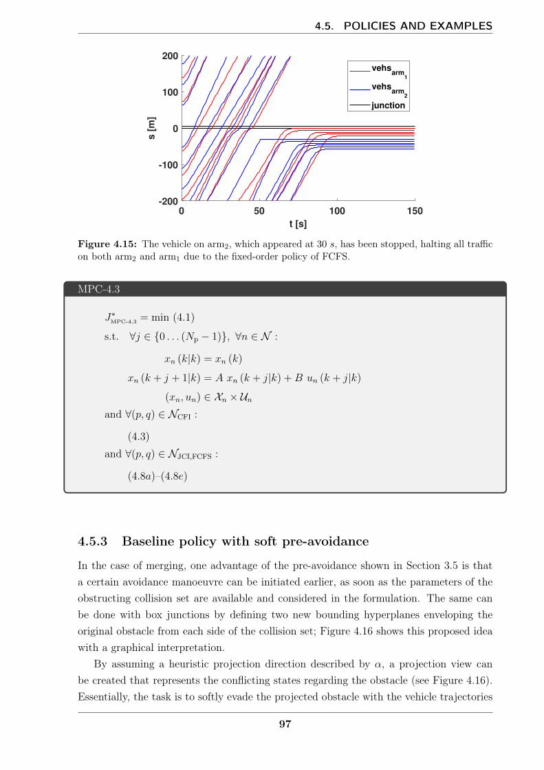
4.5. POLICIES AND EXAMPLES
0 50 100 150
t [s]
-200
-100
0
100
200
s [
m]
vehsarm
1
vehsarm
2
junction
Figure 4.15: The vehicle on arm2, which appeared at 30 s, has been stopped, halting all trafficon both arm2 and arm1 due to the fixed-order policy of FCFS.
MPC-4.3
J∗MPC-4.3 = min (4.1)
s.t. ∀j ∈ 0 . . . (Np − 1), ∀n ∈ N :
xn (k|k) = xn (k)
xn (k + j + 1|k) = A xn (k + j|k) +B un (k + j|k)
(xn, un) ∈ Xn × Unand ∀(p, q) ∈ NCFI :
(4.3)
and ∀(p, q) ∈ NJCI,FCFS :
(4.8a)–(4.8e)
4.5.3 Baseline policy with soft pre-avoidance
In the case of merging, one advantage of the pre-avoidance shown in Section 3.5 is thata certain avoidance manoeuvre can be initiated earlier, as soon as the parameters of theobstructing collision set are available and considered in the formulation. The same canbe done with box junctions by defining two new bounding hyperplanes enveloping theoriginal obstacle from each side of the collision set; Figure 4.16 shows this proposed ideawith a graphical interpretation.
By assuming a heuristic projection direction described by α, a projection view canbe created that represents the conflicting states regarding the obstacle (see Figure 4.16).Essentially, the task is to softly evade the projected obstacle with the vehicle trajectories
97
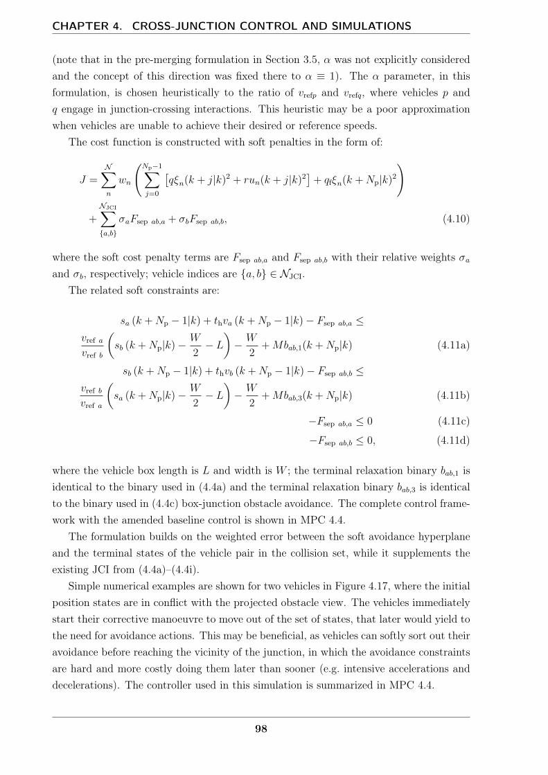
CHAPTER 4. CROSS-JUNCTION CONTROL AND SIMULATIONS
(note that in the pre-merging formulation in Section 3.5, α was not explicitly consideredand the concept of this direction was fixed there to α ≡ 1). The α parameter, in thisformulation, is chosen heuristically to the ratio of vrefp and vrefq, where vehicles p andq engage in junction-crossing interactions. This heuristic may be a poor approximationwhen vehicles are unable to achieve their desired or reference speeds.
The cost function is constructed with soft penalties in the form of:
J =N∑n
wn
(Np−1∑j=0
[qξn(k + j|k)2 + run(k + j|k)2
]+ qfξn(k +Np|k)2
)
+
NJCI∑a,b
σaFsep ab,a + σbFsep ab,b, (4.10)
where the soft cost penalty terms are Fsep ab,a and Fsep ab,b with their relative weights σaand σb, respectively; vehicle indices are a, b ∈ NJCI.
The related soft constraints are:
sa (k +Np − 1|k) + thva (k +Np − 1|k)− Fsep ab,a ≤vref avref b
(sb (k +Np|k)− W
2− L
)− W
2+Mbab,1(k +Np|k) (4.11a)
sb (k +Np − 1|k) + thvb (k +Np − 1|k)− Fsep ab,b ≤vref bvref a
(sa (k +Np|k)− W
2− L
)− W
2+Mbab,3(k +Np|k) (4.11b)
−Fsep ab,a ≤ 0 (4.11c)
−Fsep ab,b ≤ 0, (4.11d)
where the vehicle box length is L and width is W ; the terminal relaxation binary bab,1 isidentical to the binary used in (4.4a) and the terminal relaxation binary bab,3 is identicalto the binary used in (4.4c) box-junction obstacle avoidance. The complete control frame-work with the amended baseline control is shown in MPC 4.4.
The formulation builds on the weighted error between the soft avoidance hyperplaneand the terminal states of the vehicle pair in the collision set, while it supplements theexisting JCI from (4.4a)–(4.4i).
Simple numerical examples are shown for two vehicles in Figure 4.17, where the initialposition states are in conflict with the projected obstacle view. The vehicles immediatelystart their corrective manoeuvre to move out of the set of states, that later would yield tothe need for avoidance actions. This may be beneficial, as vehicles can softly sort out theiravoidance before reaching the vicinity of the junction, in which the avoidance constraintsare hard and more costly doing them later than sooner (e.g. intensive accelerations anddecelerations). The controller used in this simulation is summarized in MPC 4.4.
98

4.5. POLICIES AND EXAMPLES
Figure 4.16: Methodology of soft pre-avoidance for cross junctions, where an additional softconstraint is fitted (for both leader-follower cases) with the additional directional information ofα. This soft cost violation provides the force to move the system trajectories outward from theprojection of the junction obstacle conflict states.
MPC-4.4
J∗MPC-4.4 = min (4.10)
s.t. ∀j ∈ 0 . . . (Np − 1), ∀n ∈ N :
xn (k|k) = xn (k)
xn (k + j + 1|k) = A xn (k + j|k) +B un (k + j|k)
(xn, un) ∈ Xn × Unand ∀(p, q) ∈ NCFI :
(4.3)
and ∀p, q ∈ NJCI :
(4.4a)–(4.4i),
(4.11a)–(4.11d), with a ≡ p, b ≡ q
99
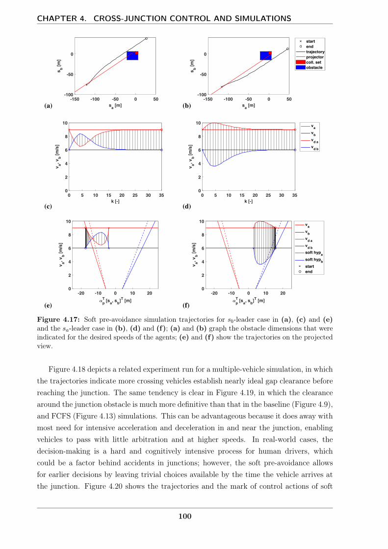
CHAPTER 4. CROSS-JUNCTION CONTROL AND SIMULATIONS
Figure 4.17: Soft pre-avoidance simulation trajectories for sb-leader case in (a), (c) and (e)and the sa-leader case in (b), (d) and (f); (a) and (b) graph the obstacle dimensions that wereindicated for the desired speeds of the agents; (e) and (f) show the trajectories on the projectedview.
Figure 4.18 depicts a related experiment run for a multiple-vehicle simulation, in whichthe trajectories indicate more crossing vehicles establish nearly ideal gap clearance beforereaching the junction. The same tendency is clear in Figure 4.19, in which the clearancearound the junction obstacle is much more definitive than that in the baseline (Figure 4.9),and FCFS (Figure 4.13) simulations. This can be advantageous because it does away withmost need for intensive acceleration and deceleration in and near the junction, enablingvehicles to pass with little arbitration and at higher speeds. In real-world cases, thedecision-making is a hard and cognitively intensive process for human drivers, whichcould be a factor behind accidents in junctions; however, the soft pre-avoidance allowsfor earlier decisions by leaving trivial choices available by the time the vehicle arrives atthe junction. Figure 4.20 shows the trajectories and the mark of control actions of soft
100
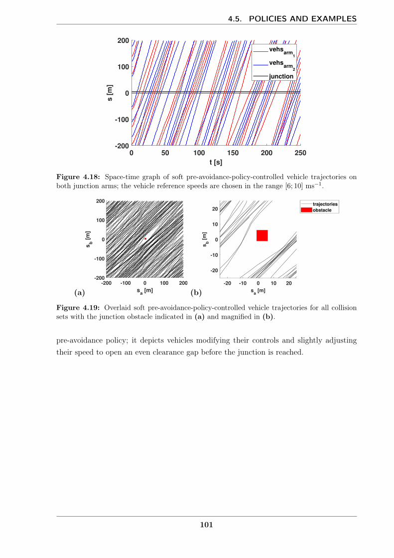
4.5. POLICIES AND EXAMPLES
0 50 100 150 200 250
t [s]
-200
-100
0
100
200
s [
m]
vehsarm
1
vehsarm
2
junction
Figure 4.18: Space-time graph of soft pre-avoidance-policy-controlled vehicle trajectories onboth junction arms; the vehicle reference speeds are chosen in the range [6; 10] ms−1.
(a)-200 -100 0 100 200
sa [m]
-200
-100
0
100
200
sb [
m]
(b)-20 -10 0 10 20
sa [m]
-20
-10
0
10
20s
b [
m]
trajectories
obstacle
Figure 4.19: Overlaid soft pre-avoidance-policy-controlled vehicle trajectories for all collisionsets with the junction obstacle indicated in (a) and magnified in (b).
pre-avoidance policy; it depicts vehicles modifying their controls and slightly adjustingtheir speed to open an even clearance gap before the junction is reached.
101
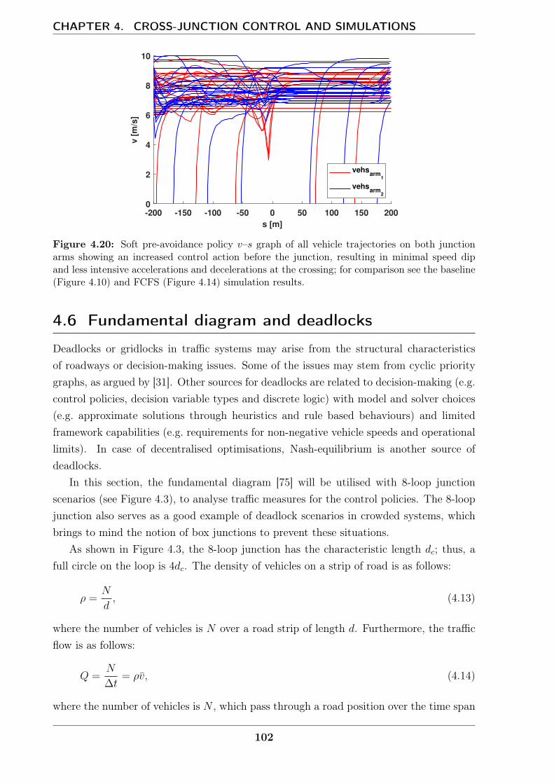
CHAPTER 4. CROSS-JUNCTION CONTROL AND SIMULATIONS
-200 -150 -100 -50 0 50 100 150 200
s [m]
0
2
4
6
8
10
v [
m/s
]
vehsarm
1
vehsarm
2
Figure 4.20: Soft pre-avoidance policy v–s graph of all vehicle trajectories on both junctionarms showing an increased control action before the junction, resulting in minimal speed dipand less intensive accelerations and decelerations at the crossing; for comparison see the baseline(Figure 4.10) and FCFS (Figure 4.14) simulation results.
4.6 Fundamental diagram and deadlocks
Deadlocks or gridlocks in traffic systems may arise from the structural characteristicsof roadways or decision-making issues. Some of the issues may stem from cyclic prioritygraphs, as argued by [31]. Other sources for deadlocks are related to decision-making (e.g.control policies, decision variable types and discrete logic) with model and solver choices(e.g. approximate solutions through heuristics and rule based behaviours) and limitedframework capabilities (e.g. requirements for non-negative vehicle speeds and operationallimits). In case of decentralised optimisations, Nash-equilibrium is another source ofdeadlocks.
In this section, the fundamental diagram [75] will be utilised with 8-loop junctionscenarios (see Figure 4.3), to analyse traffic measures for the control policies. The 8-loopjunction also serves as a good example of deadlock scenarios in crowded systems, whichbrings to mind the notion of box junctions to prevent these situations.
As shown in Figure 4.3, the 8-loop junction has the characteristic length dc; thus, afull circle on the loop is 4dc. The density of vehicles on a strip of road is as follows:
ρ =N
d, (4.13)
where the number of vehicles is N over a road strip of length d. Furthermore, the trafficflow is as follows:
Q =N
∆t= ρv, (4.14)
where the number of vehicles is N , which pass through a road position over the time span
102
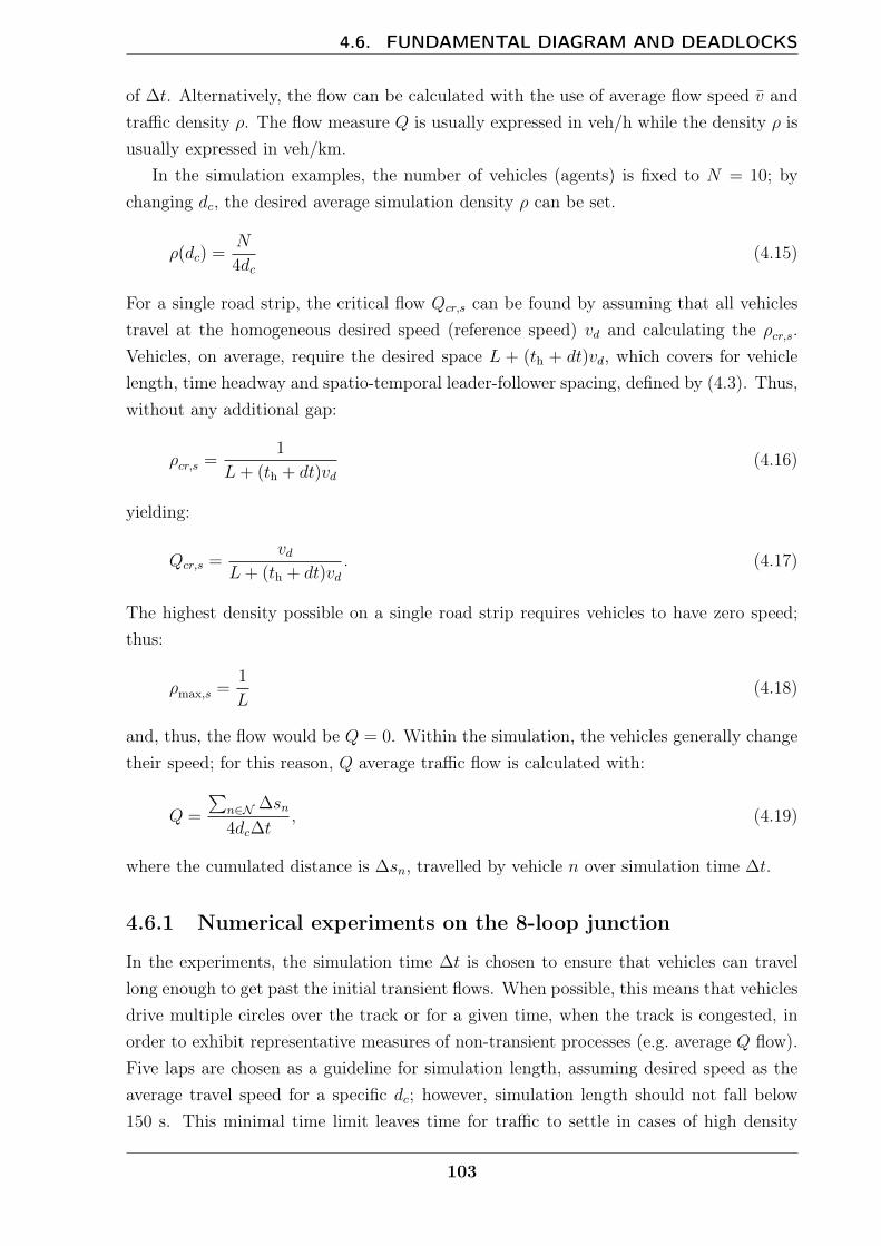
4.6. FUNDAMENTAL DIAGRAM AND DEADLOCKS
of ∆t. Alternatively, the flow can be calculated with the use of average flow speed v andtraffic density ρ. The flow measure Q is usually expressed in veh/h while the density ρ isusually expressed in veh/km.
In the simulation examples, the number of vehicles (agents) is fixed to N = 10; bychanging dc, the desired average simulation density ρ can be set.
ρ(dc) =N
4dc(4.15)
For a single road strip, the critical flow Qcr,s can be found by assuming that all vehiclestravel at the homogeneous desired speed (reference speed) vd and calculating the ρcr,s.Vehicles, on average, require the desired space L + (th + dt)vd, which covers for vehiclelength, time headway and spatio-temporal leader-follower spacing, defined by (4.3). Thus,without any additional gap:
ρcr,s =1
L+ (th + dt)vd(4.16)
yielding:
Qcr,s =vd
L+ (th + dt)vd. (4.17)
The highest density possible on a single road strip requires vehicles to have zero speed;thus:
ρmax,s =1
L(4.18)
and, thus, the flow would be Q = 0. Within the simulation, the vehicles generally changetheir speed; for this reason, Q average traffic flow is calculated with:
Q =
∑n∈N ∆sn
4dc∆t, (4.19)
where the cumulated distance is ∆sn, travelled by vehicle n over simulation time ∆t.
4.6.1 Numerical experiments on the 8-loop junction
In the experiments, the simulation time ∆t is chosen to ensure that vehicles can travellong enough to get past the initial transient flows. When possible, this means that vehiclesdrive multiple circles over the track or for a given time, when the track is congested, inorder to exhibit representative measures of non-transient processes (e.g. average Q flow).Five laps are chosen as a guideline for simulation length, assuming desired speed as theaverage travel speed for a specific dc; however, simulation length should not fall below150 s. This minimal time limit leaves time for traffic to settle in cases of high density
103
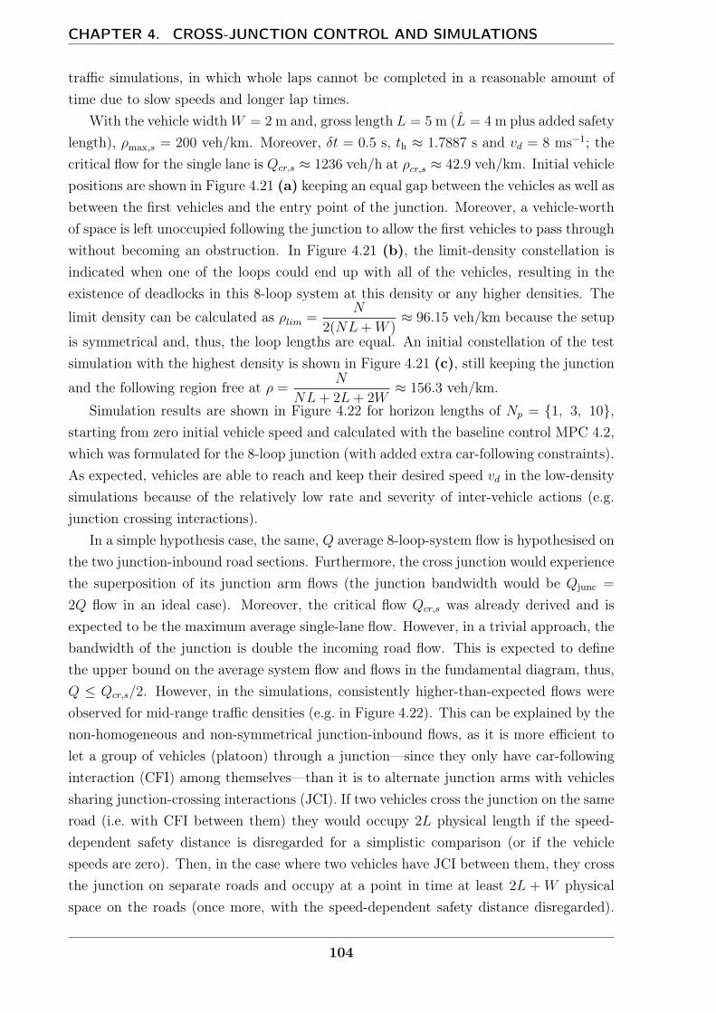
CHAPTER 4. CROSS-JUNCTION CONTROL AND SIMULATIONS
traffic simulations, in which whole laps cannot be completed in a reasonable amount oftime due to slow speeds and longer lap times.
With the vehicle widthW = 2 m and, gross length L = 5 m (L = 4 m plus added safetylength), ρmax,s = 200 veh/km. Moreover, δt = 0.5 s, th ≈ 1.7887 s and vd = 8 ms−1; thecritical flow for the single lane is Qcr,s ≈ 1236 veh/h at ρcr,s ≈ 42.9 veh/km. Initial vehiclepositions are shown in Figure 4.21 (a) keeping an equal gap between the vehicles as well asbetween the first vehicles and the entry point of the junction. Moreover, a vehicle-worthof space is left unoccupied following the junction to allow the first vehicles to pass throughwithout becoming an obstruction. In Figure 4.21 (b), the limit-density constellation isindicated when one of the loops could end up with all of the vehicles, resulting in theexistence of deadlocks in this 8-loop system at this density or any higher densities. The
limit density can be calculated as ρlim =N
2(NL+W )≈ 96.15 veh/km because the setup
is symmetrical and, thus, the loop lengths are equal. An initial constellation of the testsimulation with the highest density is shown in Figure 4.21 (c), still keeping the junction
and the following region free at ρ =N
NL+ 2L+ 2W≈ 156.3 veh/km.
Simulation results are shown in Figure 4.22 for horizon lengths of Np = 1, 3, 10,starting from zero initial vehicle speed and calculated with the baseline control MPC 4.2,which was formulated for the 8-loop junction (with added extra car-following constraints).As expected, vehicles are able to reach and keep their desired speed vd in the low-densitysimulations because of the relatively low rate and severity of inter-vehicle actions (e.g.junction crossing interactions).
In a simple hypothesis case, the same, Q average 8-loop-system flow is hypothesised onthe two junction-inbound road sections. Furthermore, the cross junction would experiencethe superposition of its junction arm flows (the junction bandwidth would be Qjunc =
2Q flow in an ideal case). Moreover, the critical flow Qcr,s was already derived and isexpected to be the maximum average single-lane flow. However, in a trivial approach, thebandwidth of the junction is double the incoming road flow. This is expected to definethe upper bound on the average system flow and flows in the fundamental diagram, thus,Q ≤ Qcr,s/2. However, in the simulations, consistently higher-than-expected flows wereobserved for mid-range traffic densities (e.g. in Figure 4.22). This can be explained by thenon-homogeneous and non-symmetrical junction-inbound flows, as it is more efficient tolet a group of vehicles (platoon) through a junction—since they only have car-followinginteraction (CFI) among themselves—than it is to alternate junction arms with vehiclessharing junction-crossing interactions (JCI). If two vehicles cross the junction on the sameroad (i.e. with CFI between them) they would occupy 2L physical length if the speed-dependent safety distance is disregarded for a simplistic comparison (or if the vehiclespeeds are zero). Then, in the case where two vehicles have JCI between them, they crossthe junction on separate roads and occupy at a point in time at least 2L + W physicalspace on the roads (once more, with the speed-dependent safety distance disregarded).
104
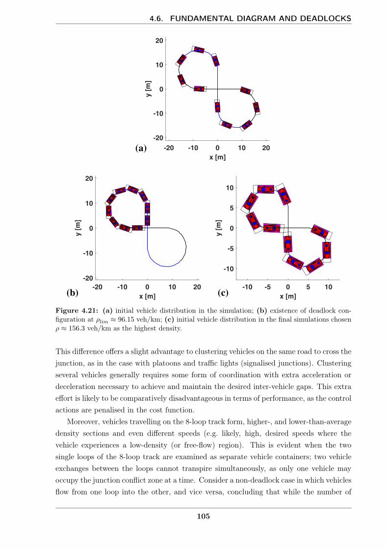
4.6. FUNDAMENTAL DIAGRAM AND DEADLOCKS
Figure 4.21: (a) initial vehicle distribution in the simulation; (b) existence of deadlock con-figuration at ρlim ≈ 96.15 veh/km; (c) initial vehicle distribution in the final simulations chosenρ ≈ 156.3 veh/km as the highest density.
This difference offers a slight advantage to clustering vehicles on the same road to cross thejunction, as in the case with platoons and traffic lights (signalised junctions). Clusteringseveral vehicles generally requires some form of coordination with extra acceleration ordeceleration necessary to achieve and maintain the desired inter-vehicle gaps. This extraeffort is likely to be comparatively disadvantageous in terms of performance, as the controlactions are penalised in the cost function.
Moreover, vehicles travelling on the 8-loop track form, higher-, and lower-than-averagedensity sections and even different speeds (e.g. likely, high, desired speeds where thevehicle experiences a low-density (or free-flow) region). This is evident when the twosingle loops of the 8-loop track are examined as separate vehicle containers; two vehicleexchanges between the loops cannot transpire simultaneously, as only one vehicle mayoccupy the junction conflict zone at a time. Consider a non-deadlock case in which vehiclesflow from one loop into the other, and vice versa, concluding that while the number of
105
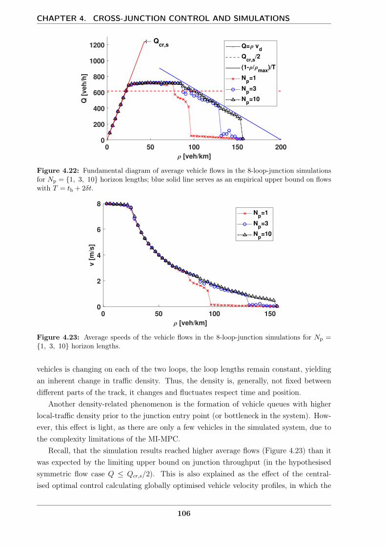
CHAPTER 4. CROSS-JUNCTION CONTROL AND SIMULATIONS
0 50 100 150 200
[veh/km]
0
200
400
600
800
1000
1200
Q [
ve
h/h
]
Qcr,s Q= v
d
Qcr,s
/2
(1- /max
)/T
Np=1
Np=3
Np=10
Figure 4.22: Fundamental diagram of average vehicle flows in the 8-loop-junction simulationsfor Np = 1, 3, 10 horizon lengths; blue solid line serves as an empirical upper bound on flowswith T = th + 2δt.
0 50 100 150
[veh/km]
0
2
4
6
8
v [
m/s
]
Np=1
Np=3
Np=10
Figure 4.23: Average speeds of the vehicle flows in the 8-loop-junction simulations for Np =1, 3, 10 horizon lengths.
vehicles is changing on each of the two loops, the loop lengths remain constant, yieldingan inherent change in traffic density. Thus, the density is, generally, not fixed betweendifferent parts of the track, it changes and fluctuates respect time and position.
Another density-related phenomenon is the formation of vehicle queues with higherlocal-traffic density prior to the junction entry point (or bottleneck in the system). How-ever, this effect is light, as there are only a few vehicles in the simulated system, due tothe complexity limitations of the MI-MPC.
Recall, that the simulation results reached higher average flows (Figure 4.23) than itwas expected by the limiting upper bound on junction throughput (in the hypothesisedsymmetric flow case Q ≤ Qcr,s/2). This is also explained as the effect of the central-ised optimal control calculating globally optimised vehicle velocity profiles, in which the
106

4.6. FUNDAMENTAL DIAGRAM AND DEADLOCKS
Figure 4.24: (a) First possible deadlock configuration at ρ ≈ 96.87 veh/km for Np = 1; (b)deadlock configuration at ρ ≈ 140 veh/km.
optimiser is able to exploit local density differences, non-symmetric and non-stationaryflows to reach more efficient higher average flows than the hypothesised limit.
In the high-traffic-density region, the vehicles can only maintain lower-average speedsdue to the high interactions between them and the low availability of inter-vehicle gaps.The interesting fact is that, over the ρlim limit density, the simulation may end up ina deadlock situation; however, for longer prediction horizons the simulations remainedoperational above the limit density. This shows the resilience of predictive control againstsimple trivial deadlocks.
In Figure 4.22, the lower Q flow values in the high-density region correspond to thedeadlock situations; these flows are non-zero, because between the initial configuration andthe deadlock configurations the vehicles cover a non-zero distance, resulting in non-zeroaverage measures. These deadlock situation, however, easily identifiable from the averagemeasures because they discontinuously jump to a low value (e.g. in the fundamentaldiagrams). Figure 4.23 shows the average flow speeds for the three horizon lengths Np =
1, 3, 10, reaching the desired speed at the low-density simulations and reaching near-zero speed at the simulations experiencing the high-density deadlock configurations. ForNp = 1, Figure 4.24 (a) shows the deadlock configuration at ρ ≈ 96.87 veh/km, whichis in line with ρ > ρlim. Furthermore, this shows that the vehicles with short predictivecapabilities are more prone to end up in deadlock situations. Figure 4.24 (b) shows adeadlock in a denser traffic simulation at ρ ≈ 140 veh/km which would require moreforesight and fairness between vehicles to prevent.
As discussed in Section 4.3.2, the 8-loop road structure is formulated on the straightroad core simulation, with two extra car-following constraints and visualised as a projec-tion to the 8-loop (see Figure 4.3). To test the control policies from Section 4.5, simplythe extra car-following constraints need to be added which does not change the structureof the controller. Thus, the FCFS MPC 4.3 and soft pre-avoidance MPC 4.4 policies are
107

CHAPTER 4. CROSS-JUNCTION CONTROL AND SIMULATIONS
(a) (b)
Figure 4.25: Baseline, FCFS, and soft pre-avoidance 8-loop-junction simulations for Np = 5horizon length; (a) fundamental diagram; (b) average vehicle flow speeds; blue solid line is servesas an empirical upper bound on flows with T = th + 2δt.
compatible with the 8-loop simulation type similarly as the previous baseline examplewith MPC 4.2. The FCFS crossing orders (priorities) are decided at dc characteristicdistance from the centre of the junction same as in Section 4.5.2. The average flow andflow speeds, and densities are shown in Figure 4.25 with Np = 5 horizon length to enablecomparison between the baseline, FCFS, and soft pre-avoidance policy simulations. Allthree policies largely performed similarly, though the FCFS did sometimes achieve loweroperational flows than the other two controls. However, FCFS is the only policy whichdid not result in a deadlock breakdown until reaching the highest density scenario (whichwas explicitly designed to result in deadlock configuration). This resilience and the lowerflows come from the fact that it heuristically fixes vehicle-crossing order in advance ofthe junction; the inferior adaptability of the FCFS controller in terms of crossing orderensures that bad traffic choices that lead to deadlocks and could not be forecast by thecontrol are not made.
4.6.2 Passing completion in the box junction
Box junctions are popular in areas where traffic is highly susceptible to deadlocks, grid-locks due to local traffic specific properties (e.g. due to low visibility, high density, orasymmetric traffic inflows). There are two main approaches: impose a minimal speedacross the junction, as discussed in [3] and formulated with time-headway safety in Sec-tion 3.6; or demand the vehicle to be in front of or past the crossing area in the foreseeablefuture, practically implementing a hysteresis switch [18]. According to de Campos et al.[18], the problem is manually split into two sub-problems seeking the better option toeither cross or not cross the conflicting road section when another vehicle also aims todo the same; the considered vehicle orders were a heuristic subset of all possible cross-ing orders in the decision-making problem. Furthermore, each sub-problem-calculationsequence is repeated in the usual receding-horizon manner of MPCs. The minimal speedrequirement seen in [3] does not provide the emergency stop capability in the region.
108
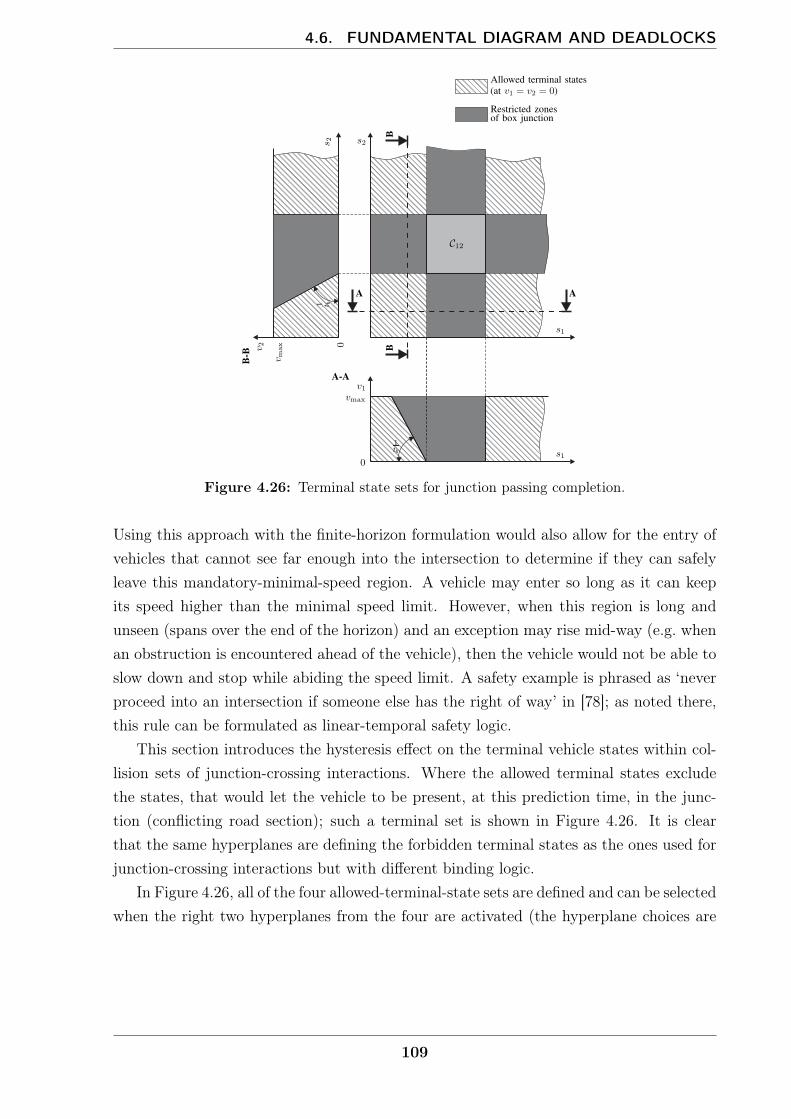
4.6. FUNDAMENTAL DIAGRAM AND DEADLOCKS
Figure 4.26: Terminal state sets for junction passing completion.
Using this approach with the finite-horizon formulation would also allow for the entry ofvehicles that cannot see far enough into the intersection to determine if they can safelyleave this mandatory-minimal-speed region. A vehicle may enter so long as it can keepits speed higher than the minimal speed limit. However, when this region is long andunseen (spans over the end of the horizon) and an exception may rise mid-way (e.g. whenan obstruction is encountered ahead of the vehicle), then the vehicle would not be able toslow down and stop while abiding the speed limit. A safety example is phrased as ‘neverproceed into an intersection if someone else has the right of way’ in [78]; as noted there,this rule can be formulated as linear-temporal safety logic.
This section introduces the hysteresis effect on the terminal vehicle states within col-lision sets of junction-crossing interactions. Where the allowed terminal states excludethe states, that would let the vehicle to be present, at this prediction time, in the junc-tion (conflicting road section); such a terminal set is shown in Figure 4.26. It is clearthat the same hyperplanes are defining the forbidden terminal states as the ones used forjunction-crossing interactions but with different binding logic.
In Figure 4.26, all of the four allowed-terminal-state sets are defined and can be selectedwhen the right two hyperplanes from the four are activated (the hyperplane choices are
109
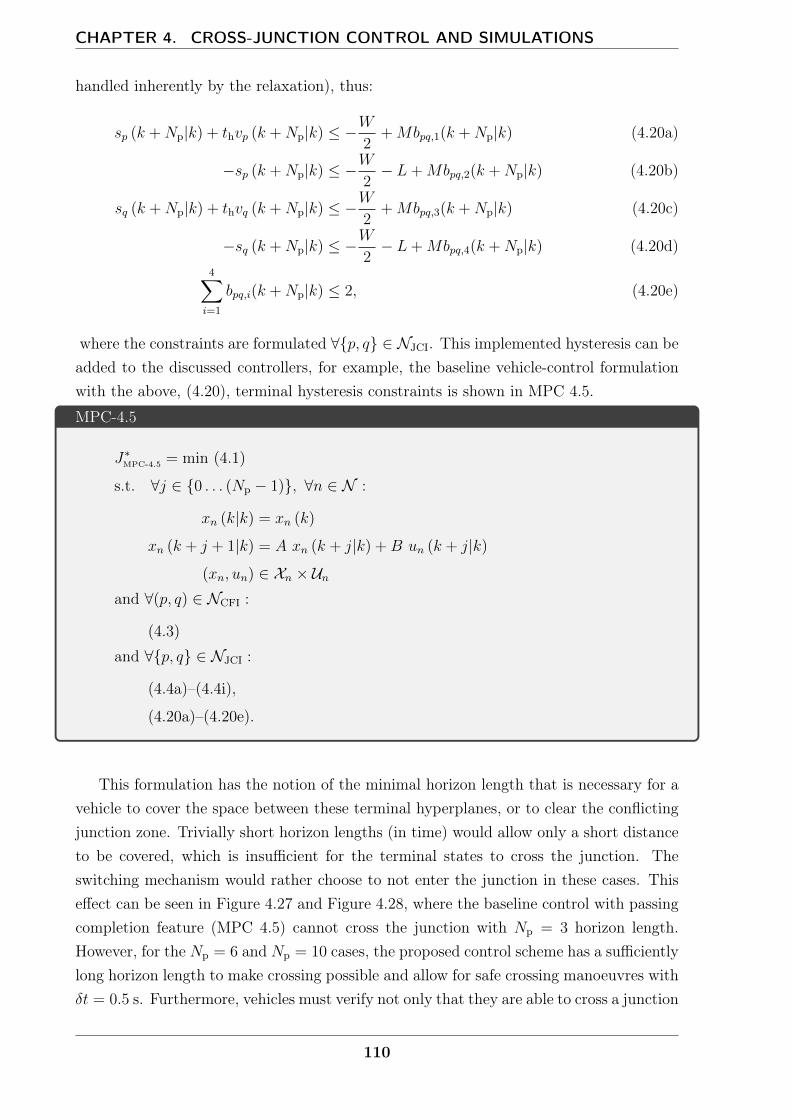
CHAPTER 4. CROSS-JUNCTION CONTROL AND SIMULATIONS
handled inherently by the relaxation), thus:
sp (k +Np|k) + thvp (k +Np|k) ≤ −W2
+Mbpq,1(k +Np|k) (4.20a)
−sp (k +Np|k) ≤ −W2− L+Mbpq,2(k +Np|k) (4.20b)
sq (k +Np|k) + thvq (k +Np|k) ≤ −W2
+Mbpq,3(k +Np|k) (4.20c)
−sq (k +Np|k) ≤ −W2− L+Mbpq,4(k +Np|k) (4.20d)
4∑i=1
bpq,i(k +Np|k) ≤ 2, (4.20e)
where the constraints are formulated ∀p, q ∈ NJCI. This implemented hysteresis can beadded to the discussed controllers, for example, the baseline vehicle-control formulationwith the above, (4.20), terminal hysteresis constraints is shown in MPC 4.5.
MPC-4.5
J∗MPC-4.5 = min (4.1)
s.t. ∀j ∈ 0 . . . (Np − 1), ∀n ∈ N :
xn (k|k) = xn (k)
xn (k + j + 1|k) = A xn (k + j|k) +B un (k + j|k)
(xn, un) ∈ Xn × Unand ∀(p, q) ∈ NCFI :
(4.3)
and ∀p, q ∈ NJCI :
(4.4a)–(4.4i),
(4.20a)–(4.20e).
This formulation has the notion of the minimal horizon length that is necessary for avehicle to cover the space between these terminal hyperplanes, or to clear the conflictingjunction zone. Trivially short horizon lengths (in time) would allow only a short distanceto be covered, which is insufficient for the terminal states to cross the junction. Theswitching mechanism would rather choose to not enter the junction in these cases. Thiseffect can be seen in Figure 4.27 and Figure 4.28, where the baseline control with passingcompletion feature (MPC 4.5) cannot cross the junction with Np = 3 horizon length.However, for the Np = 6 and Np = 10 cases, the proposed control scheme has a sufficientlylong horizon length to make crossing possible and allow for safe crossing manoeuvres withδt = 0.5 s. Furthermore, vehicles must verify not only that they are able to cross a junction
110
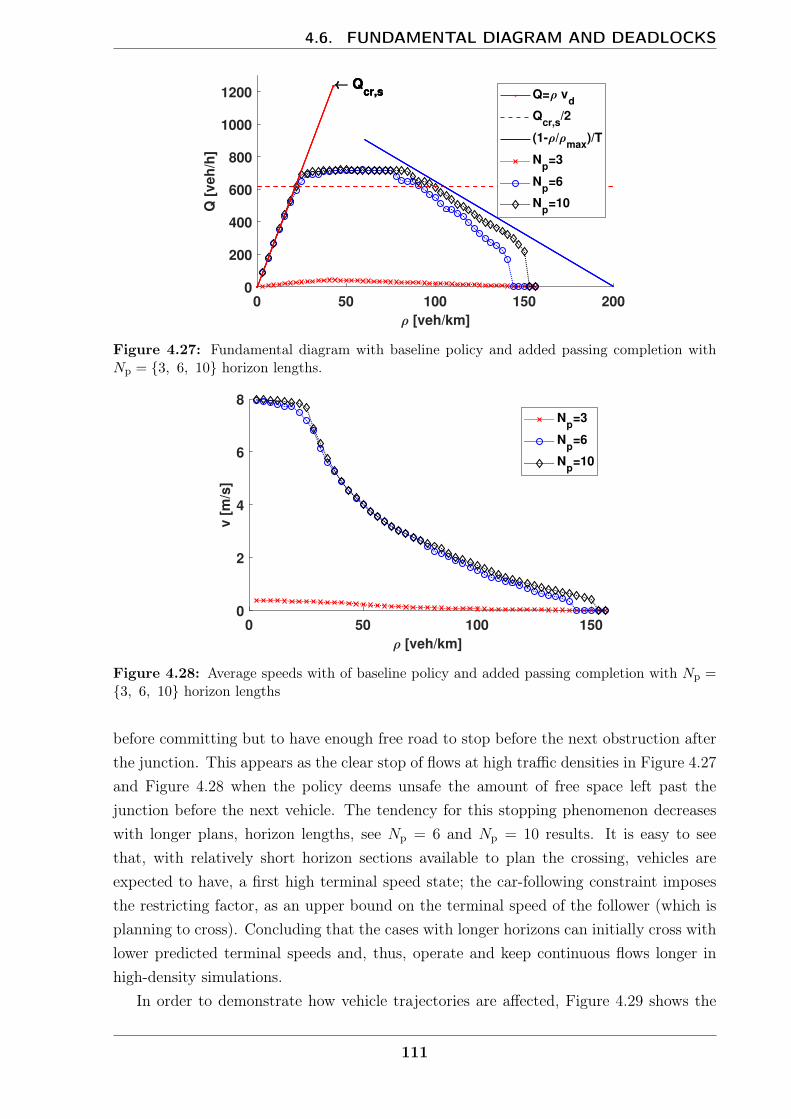
4.6. FUNDAMENTAL DIAGRAM AND DEADLOCKS
0 50 100 150 200
[veh/km]
0
200
400
600
800
1000
1200
Q [
ve
h/h
]
Qcr,s
Qcr,s
Qcr,s Q= v
d
Qcr,s
/2
(1- /max
)/T
Np=3
Np=6
Np=10
Figure 4.27: Fundamental diagram with baseline policy and added passing completion withNp = 3, 6, 10 horizon lengths.
0 50 100 150
[veh/km]
0
2
4
6
8
v [
m/s
]
Np=3
Np=6
Np=10
Figure 4.28: Average speeds with of baseline policy and added passing completion with Np =3, 6, 10 horizon lengths
before committing but to have enough free road to stop before the next obstruction afterthe junction. This appears as the clear stop of flows at high traffic densities in Figure 4.27and Figure 4.28 when the policy deems unsafe the amount of free space left past thejunction before the next vehicle. The tendency for this stopping phenomenon decreaseswith longer plans, horizon lengths, see Np = 6 and Np = 10 results. It is easy to seethat, with relatively short horizon sections available to plan the crossing, vehicles areexpected to have, a first high terminal speed state; the car-following constraint imposesthe restricting factor, as an upper bound on the terminal speed of the follower (which isplanning to cross). Concluding that the cases with longer horizons can initially cross withlower predicted terminal speeds and, thus, operate and keep continuous flows longer inhigh-density simulations.
In order to demonstrate how vehicle trajectories are affected, Figure 4.29 shows the
111
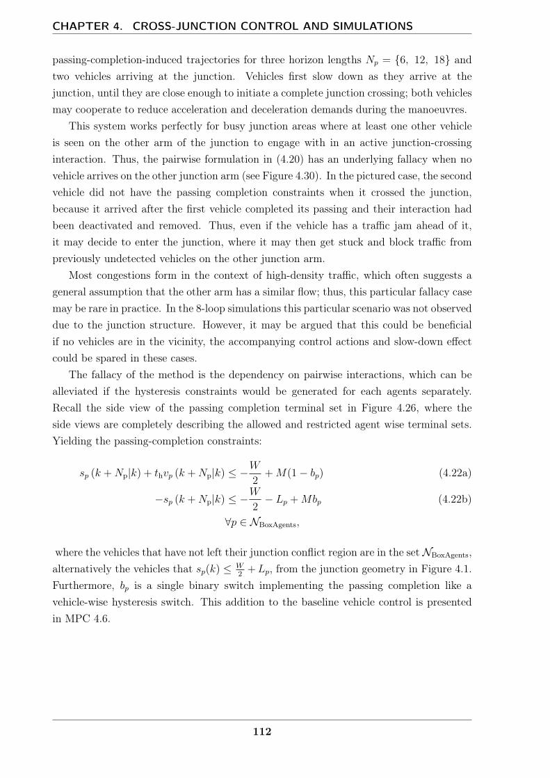
CHAPTER 4. CROSS-JUNCTION CONTROL AND SIMULATIONS
passing-completion-induced trajectories for three horizon lengths Np = 6, 12, 18 andtwo vehicles arriving at the junction. Vehicles first slow down as they arrive at thejunction, until they are close enough to initiate a complete junction crossing; both vehiclesmay cooperate to reduce acceleration and deceleration demands during the manoeuvres.
This system works perfectly for busy junction areas where at least one other vehicleis seen on the other arm of the junction to engage with in an active junction-crossinginteraction. Thus, the pairwise formulation in (4.20) has an underlying fallacy when novehicle arrives on the other junction arm (see Figure 4.30). In the pictured case, the secondvehicle did not have the passing completion constraints when it crossed the junction,because it arrived after the first vehicle completed its passing and their interaction hadbeen deactivated and removed. Thus, even if the vehicle has a traffic jam ahead of it,it may decide to enter the junction, where it may then get stuck and block traffic frompreviously undetected vehicles on the other junction arm.
Most congestions form in the context of high-density traffic, which often suggests ageneral assumption that the other arm has a similar flow; thus, this particular fallacy casemay be rare in practice. In the 8-loop simulations this particular scenario was not observeddue to the junction structure. However, it may be argued that this could be beneficialif no vehicles are in the vicinity, the accompanying control actions and slow-down effectcould be spared in these cases.
The fallacy of the method is the dependency on pairwise interactions, which can bealleviated if the hysteresis constraints would be generated for each agents separately.Recall the side view of the passing completion terminal set in Figure 4.26, where theside views are completely describing the allowed and restricted agent wise terminal sets.Yielding the passing-completion constraints:
sp (k +Np|k) + thvp (k +Np|k) ≤ −W2
+M(1− bp) (4.22a)
−sp (k +Np|k) ≤ −W2− Lp +Mbp (4.22b)
∀p ∈ NBoxAgents,
where the vehicles that have not left their junction conflict region are in the setNBoxAgents,alternatively the vehicles that sp(k) ≤ W
2+Lp, from the junction geometry in Figure 4.1.
Furthermore, bp is a single binary switch implementing the passing completion like avehicle-wise hysteresis switch. This addition to the baseline vehicle control is presentedin MPC 4.6.
112

4.6. FUNDAMENTAL DIAGRAM AND DEADLOCKS
MPC-4.6
J∗MPC-4.6 = min (4.1)
s.t. ∀j ∈ 0 . . . (Np − 1), ∀n ∈ N :
xn (k|k) = xn (k)
xn (k + j + 1|k) = A xn (k + j|k) +B un (k + j|k)
(xn, un) ∈ Xn × Unand ∀(p, q) ∈ NCFI :
(4.3)
and ∀p, q ∈ NJCI :
(4.4a)–(4.4i),
and ∀p ∈ NBoxAgents :
(4.22a)–(4.22b),
Finally, Figure 4.31 shows the cases with and without the passing-completion con-straints added. In a normal case with a bigger gap in the competing traffic flow, theoptimiser would take the chance and make a vehicle waiting for its right of way enterthe intersection even if there is a traffic jam ahead of it. This is a valid move because,at that moment, the vehicle would not make other vehicles suffer (i.e. it would not in-crease the aggregated cost of the objective function but lower it because it can get closerto its destination). It is easy to see that after other vehicles appear, this move provesto be counter-productive. In contrast, when the passing-completion constraint is added,the vehicle remains in front of the junction until it can safely and completely cross; thusallowing uninterrupted traffic on the other arm.
113

CHAPTER 4. CROSS-JUNCTION CONTROL AND SIMULATIONS
(a)-100 -50 0 50 100
s [m]
0
2
4
6
8
10
v [
m/s
]
Np=6
junction
veh1 traj
veh1 tail
veh2 traj
veh2 tail
(b)-100 -50 0 50 100
s1 [m]
-100
-50
0
50
100
s2 [
m]
Np=6
trajectory
obstacle
(c)-100 -50 0 50 100
s [m]
0
2
4
6
8
10
v [
m/s
]
Np=12
junction
veh1 traj
veh1 tail
veh2 traj
veh2 tail
(d)-100 -50 0 50 100
s1 [m]
-100
-50
0
50
100
s2 [
m]
Np=12
trajectory
obstacle
(e)-100 -50 0 50 100
s [m]
0
2
4
6
8
10
v [
m/s
]
Np=18
junction
veh1 traj
veh1 tail
veh2 traj
veh2 tail
(f)-100 -50 0 50 100
s1 [m]
-100
-50
0
50
100
s2 [
m]
Np=18
trajectory
obstacle
Figure 4.29: Passing completion of trajectories for Np = 6, 12, 18 horizon steps; the leftside depicts speed–position graphs while the right side shows the related collision set graphs fortwo vehicles approaching the junction on different arms.
114
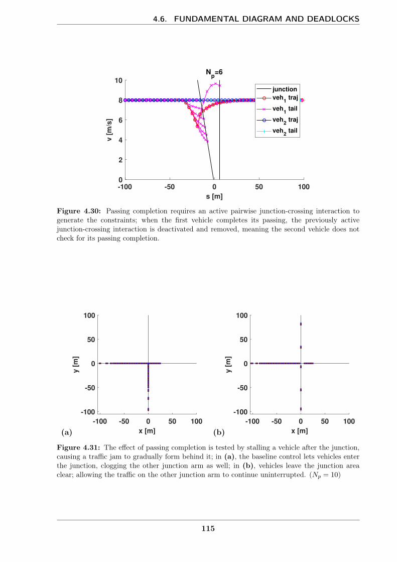
4.6. FUNDAMENTAL DIAGRAM AND DEADLOCKS
-100 -50 0 50 100
s [m]
0
2
4
6
8
10
v [
m/s
]
Np=6
junction
veh1 traj
veh1 tail
veh2 traj
veh2 tail
Figure 4.30: Passing completion requires an active pairwise junction-crossing interaction togenerate the constraints; when the first vehicle completes its passing, the previously activejunction-crossing interaction is deactivated and removed, meaning the second vehicle does notcheck for its passing completion.
(a)-100 -50 0 50 100
x [m]
-100
-50
0
50
100
y [
m]
(b)-100 -50 0 50 100
x [m]
-100
-50
0
50
100
y [
m]
Figure 4.31: The effect of passing completion is tested by stalling a vehicle after the junction,causing a traffic jam to gradually form behind it; in (a), the baseline control lets vehicles enterthe junction, clogging the other junction arm as well; in (b), vehicles leave the junction areaclear; allowing the traffic on the other junction arm to continue uninterrupted. (Np = 10)
115
CHAPTER 4. CROSS-JUNCTION CONTROL AND SIMULATIONS
4.7 Summary
This chapter has shown numerical simulations of multi-agent vehicle control for threepolicies. The baseline policy allows for junction crossing order changes and adaptation tolate information. The FCFS fixed-junction-passing-order policy encodes lower computa-tional complexity as a trade for adaptation, since it is a heuristic type approach with fewerbinaries needed in the optimisation. The soft pre-avoidance policy aligns vehicles earlyon to pass the conflicting junction zone without heavy interaction (i.e. acceleration anddeceleration) near the junction. Traffic measures were demonstrated on fundamental dia-grams to compare 8-loop-junction simulations. Data shows that the chance of deadlocksituations are mitigated with longer optimisation horizons, which were clearly demon-strated on a fundamental diagram with baseline control. Finally, box junction rule wasimplemented and demonstrated with passing-completion-terminal constraints for pair-and agent-wise formulations (i.e. do not enter the conflicting intersection region if, by theterminal state, the vehicle cannot exit it).
116
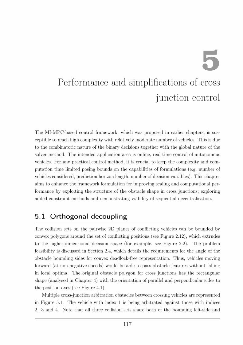
5Performance and simplifications of cross
junction control
The MI-MPC-based control framework, which was proposed in earlier chapters, is sus-ceptible to reach high complexity with relatively moderate number of vehicles. This is dueto the combinatoric nature of the binary decisions together with the global nature of thesolver method. The intended application area is online, real-time control of autonomousvehicles. For any practical control method, it is crucial to keep the complexity and com-putation time limited posing bounds on the capabilities of formulations (e.g. number ofvehicles considered, prediction horizon length, number of decision variables). This chapteraims to enhance the framework formulation for improving scaling and computational per-formance by exploiting the structure of the obstacle shape in cross junctions; exploringadded constraint methods and demonstrating viability of sequential decentralisation.
5.1 Orthogonal decoupling
The collision sets on the pairwise 2D planes of conflicting vehicles can be bounded byconvex polygons around the set of conflicting positions (see Figure 2.12), which extrudesto the higher-dimensional decision space (for example, see Figure 2.2). The problemfeasibility is discussed in Section 2.4, which details the requirements for the angle of theobstacle bounding sides for convex deadlock-free representation. Thus, vehicles movingforward (at non-negative speeds) would be able to pass obstacle features without fallingin local optima. The original obstacle polygon for cross junctions has the rectangularshape (analysed in Chapter 4) with the orientation of parallel and perpendicular sides tothe position axes (see Figure 4.1).
Multiple cross-junction arbitration obstacles between crossing vehicles are representedin Figure 5.1. The vehicle with index 1 is being arbitrated against those with indices2, 3 and 4. Note that all three collision sets share both of the bounding left-side and
117
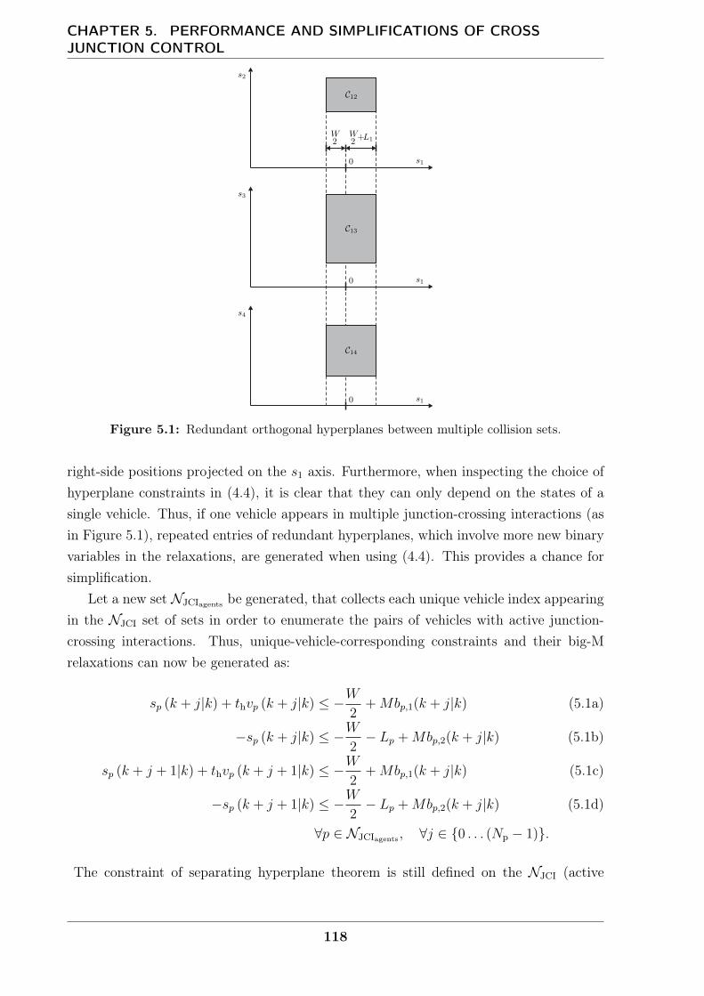
CHAPTER 5. PERFORMANCE AND SIMPLIFICATIONS OF CROSSJUNCTION CONTROL
Figure 5.1: Redundant orthogonal hyperplanes between multiple collision sets.
right-side positions projected on the s1 axis. Furthermore, when inspecting the choice ofhyperplane constraints in (4.4), it is clear that they can only depend on the states of asingle vehicle. Thus, if one vehicle appears in multiple junction-crossing interactions (asin Figure 5.1), repeated entries of redundant hyperplanes, which involve more new binaryvariables in the relaxations, are generated when using (4.4). This provides a chance forsimplification.
Let a new set NJCIagents be generated, that collects each unique vehicle index appearingin the NJCI set of sets in order to enumerate the pairs of vehicles with active junction-crossing interactions. Thus, unique-vehicle-corresponding constraints and their big-Mrelaxations can now be generated as:
sp (k + j|k) + thvp (k + j|k) ≤ −W2
+Mbp,1(k + j|k) (5.1a)
−sp (k + j|k) ≤ −W2− Lp +Mbp,2(k + j|k) (5.1b)
sp (k + j + 1|k) + thvp (k + j + 1|k) ≤ −W2
+Mbp,1(k + j|k) (5.1c)
−sp (k + j + 1|k) ≤ −W2− Lp +Mbp,2(k + j|k) (5.1d)
∀p ∈ NJCIagents , ∀j ∈ 0 . . . (Np − 1).
The constraint of separating hyperplane theorem is still defined on the NJCI (active
118
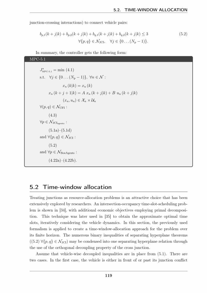
5.2. TIME-WINDOW ALLOCATION
junction-crossing interactions) to connect vehicle pairs:
bp,1(k + j|k) + bp,2(k + j|k) + bq,1(k + j|k) + bq,2(k + j|k) ≤ 3 (5.2)
∀p, q ∈ NJCI, ∀j ∈ 0 . . . (Np − 1).
In summary, the controller gets the following form:MPC-5.1
J∗MPC-5.1 = min (4.1)
s.t. ∀j ∈ 0 . . . (Np − 1), ∀n ∈ N :
xn (k|k) = xn (k)
xn (k + j + 1|k) = A xn (k + j|k) +B un (k + j|k)
(xn, un) ∈ Xn × Un∀(p, q) ∈ NCFI :
(4.3)
∀p ∈ NJCIagents :
(5.1a)–(5.1d)
and ∀p, q ∈ NJCI :
(5.2)
and ∀p ∈ NBoxAgents :
(4.22a)–(4.22b).
5.2 Time-window allocation
Treating junctions as resource-allocation problems is an attractive choice that has beenextensively explored by researchers. An intersection-occupancy time-slot-scheduling prob-lem is shown in [34], with additional economic objectives employing primal decomposi-tion. This technique was later used in [35] to obtain the approximate optimal timeslots, iteratively considering the vehicle dynamics. In this section, the previously usedformalism is applied to create a time-window-allocation approach for the problem overits finite horizon. The numerous binary inequalities of separating hyperplane theorems((5.2) ∀p, q ∈ NJCI) may be condensed into one separating hyperplane relation throughthe use of the orthogonal decoupling property of the cross junction.
Assume that vehicle-wise decoupled inequalities are in place from (5.1). There aretwo cases. In the first case, the vehicle is either in front of or past its junction conflict
119

CHAPTER 5. PERFORMANCE AND SIMPLIFICATIONS OF CROSSJUNCTION CONTROL
region. This case concludes that one of the two hyperplanes must be active (non-relaxed),in terms of binaries:
bp,1(k + j|k) + bp,2(k + j|k) = 1. (5.4)
In the second case, suppose that if a vehicle is allowed to occupy the shared road sectionwithin the junction, it would need to relax both of its safety hyperplanes:
bp,1(k + j|k) + bp,2(k + j|k) = 2. (5.5)
Now, consider that only one vehicle can safely have the right of way in the junction atany one time; thus, all other vehicles must remain outside of the junction conflict region,yielding:∑
p∈NJCIagents
bp,1(k + j|k) + bp,2(k + j|k) = (NJCIagents − 1) + 2
or, alternatively expressed with an inequality:∑p∈NJCIagents
bp,1(k + j|k) + bp,2(k + j|k) ≤ (NJCIagents − 1) + 2, (5.6)
where the number of vehicles is NJCIagents in the set of NJCIagents.This separating hyperplane theorem implements a junction-crossing sequencing as
though it were resource allocation of a shared medium (junction). However, it is more thana simple resource allocation; this formulation can readily incorporate vehicle dynamics,time-headway safety, operating limits and any other constraints that preserve the problemstructure. Moreover, in this decision-making, the consideration of vehicle cooperation isdirectly incorporated through the optimised cost of the aggregated objective function.Figure 5.2 shows the allocated discrete time windows; each time window can only occupya given time span alone. The structure of the corner-cutting prevention inflates the sizeof the time windows to prevent junction entry between the discrete time steps while theconstraints are only defined at the discrete time steps.
The final forms of the time-window constraints for the MPC are summarised inMPC 5.2.
120
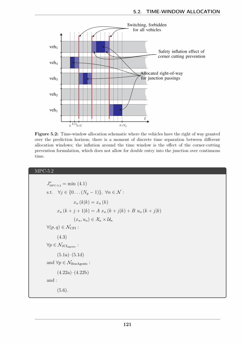
5.2. TIME-WINDOW ALLOCATION
Figure 5.2: Time-window allocation schematic where the vehicles have the right of way grantedover the prediction horizon; there is a moment of discrete time separation between differentallocation windows; the inflation around the time window is the effect of the corner-cuttingprevention formulation, which does not allow for double entry into the junction over continuoustime.
MPC-5.2
J∗MPC-5.2 = min (4.1)
s.t. ∀j ∈ 0 . . . (Np − 1), ∀n ∈ N :
xn (k|k) = xn (k)
xn (k + j + 1|k) = A xn (k + j|k) +B un (k + j|k)
(xn, un) ∈ Xn × Un∀(p, q) ∈ NCFI :
(4.3)
∀p ∈ NJCIagents :
(5.1a)–(5.1d)
and ∀p ∈ NBoxAgents :
(4.22a)–(4.22b)
and :
(5.6).
121
CHAPTER 5. PERFORMANCE AND SIMPLIFICATIONS OF CROSSJUNCTION CONTROL
5.3 Numerical tests of formulations
In this section, three numerical 8-loop simulations will be compared—MPC 4.5, MPC 5.1and MPC 5.2. MPC 4.5 is the un-simplified (US) baseline vehicle-control formulationwith passing completion hysteresis; MPC 5.1 is the formulation of the orthogonal de-coupling (OD) from Section 5.1; MPC 5.2 is the time-window (TW) allocation fromSection 5.2. The characteristic length dc was chosen to attain the desired traffic dens-
ities ρ = 50, 100, 120 vehkm
for N = 10 vehicles in the 8-loop junction. The simula-tions were deterministic; they started from the same initial states and ran for all threevehicular controls with each new parameter value. The simulated time was chosen tobe 10 minutes (= 600 s) with δt = 0.5 s. Moreover, the deadlock-averting or box-junction-implementing terminal junction-passing-completion constraints were added forall formulations. The un-simplified formulation is the baseline problem with (4.4) junc-tion constraints and (4.20) box-junction passing completion. The orthogonal decouplingis a simplified formulation composed of the (5.1) agent-wise junction constraints coupledwith the (5.2) binary separating-hyperplane constraints of and the (4.22) agent-wise box-junction implementation. The time-window allocation is based on the (5.1) agent-wisejunction constraints coupled with the (5.6) binary separating-hyperplane inequality andthe (4.22) agent-wise box-junction implementation.
A distance measure was used to analyse whether decisions are the same or differentacross formulations. Simulation similarity was evaluated through a comparison of vehicletrajectories between run pairs. The comparison was done through a cumulated squaredposition error measure:
ε =∑n∈N
[kmax∑k=0
(ssim an (k)− ssim b
n (k))2
] 12
, (5.8)
where the maximum number of discrete simulation time steps is kmax and the simula-tion results sim a and sim b are compared and stored for post-processing. Alternatively,differences between trajectories may be identified by looking at the average flow Q meas-ures, which depend on the distances travelled by vehicles and are presented in Table 5.1,Table 5.2 and Table 5.3. A dissimilar trajectory simulation is shown in Figure 5.3, whichpresents a single selected trajectory across the two simulations, where Q average flow wasalso different.
It was determined that trajectories with a short horizon control and low traffic density
(Np = 6 and ρ = 50vehkm
) yield a low number of interactions (trajectory changes due toobstacle avoidance) in the simulations; the trajectories were identical for all three methodsin this region (US, OD and TW). With the same horizon length, however, only the US
and OD formulations remained close to one another (i.e. ρ = 100vehkm
: ε ≈ 0.0081 and ρ =
122
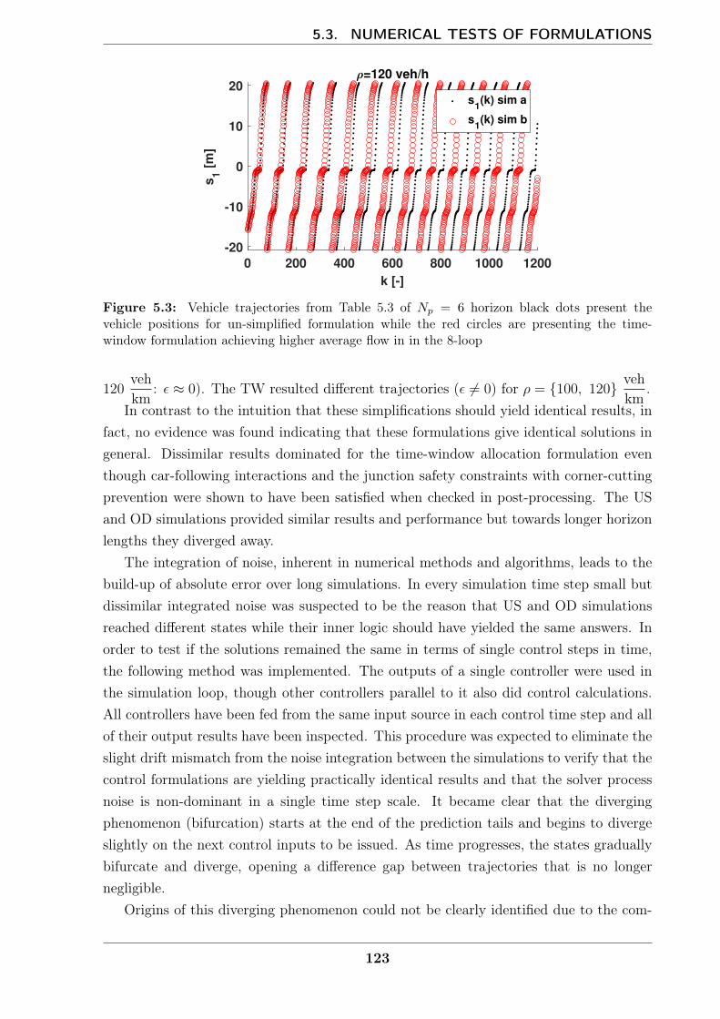
5.3. NUMERICAL TESTS OF FORMULATIONS
0 200 400 600 800 1000 1200
k [-]
-20
-10
0
10
20
s1 [
m]
=120 veh/h
s1(k) sim a
s1(k) sim b
Figure 5.3: Vehicle trajectories from Table 5.3 of Np = 6 horizon black dots present thevehicle positions for un-simplified formulation while the red circles are presenting the time-window formulation achieving higher average flow in in the 8-loop
120vehkm
: ε ≈ 0). The TW resulted different trajectories (ε 6= 0) for ρ = 100, 120 vehkm
.In contrast to the intuition that these simplifications should yield identical results, in
fact, no evidence was found indicating that these formulations give identical solutions ingeneral. Dissimilar results dominated for the time-window allocation formulation eventhough car-following interactions and the junction safety constraints with corner-cuttingprevention were shown to have been satisfied when checked in post-processing. The USand OD simulations provided similar results and performance but towards longer horizonlengths they diverged away.
The integration of noise, inherent in numerical methods and algorithms, leads to thebuild-up of absolute error over long simulations. In every simulation time step small butdissimilar integrated noise was suspected to be the reason that US and OD simulationsreached different states while their inner logic should have yielded the same answers. Inorder to test if the solutions remained the same in terms of single control steps in time,the following method was implemented. The outputs of a single controller were used inthe simulation loop, though other controllers parallel to it also did control calculations.All controllers have been fed from the same input source in each control time step and allof their output results have been inspected. This procedure was expected to eliminate theslight drift mismatch from the noise integration between the simulations to verify that thecontrol formulations are yielding practically identical results and that the solver processnoise is non-dominant in a single time step scale. It became clear that the divergingphenomenon (bifurcation) starts at the end of the prediction tails and begins to divergeslightly on the next control inputs to be issued. As time progresses, the states graduallybifurcate and diverge, opening a difference gap between trajectories that is no longernegligible.
Origins of this diverging phenomenon could not be clearly identified due to the com-
123
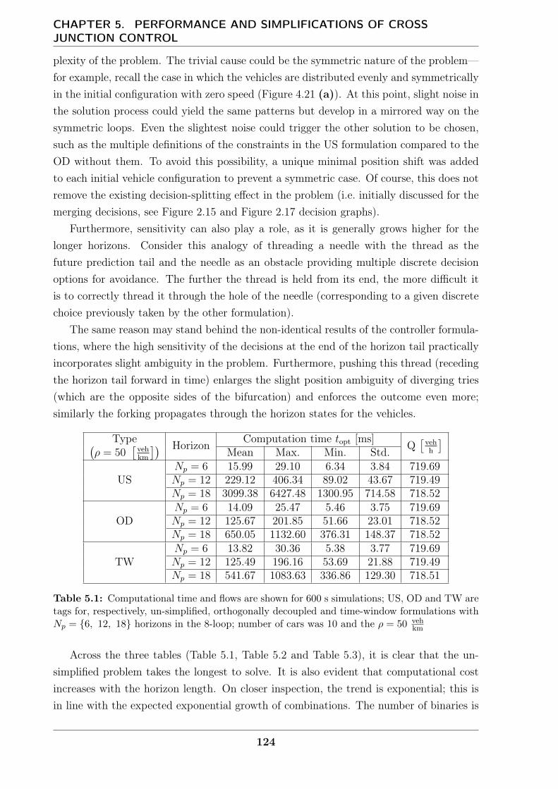
CHAPTER 5. PERFORMANCE AND SIMPLIFICATIONS OF CROSSJUNCTION CONTROL
plexity of the problem. The trivial cause could be the symmetric nature of the problem—for example, recall the case in which the vehicles are distributed evenly and symmetricallyin the initial configuration with zero speed (Figure 4.21 (a)). At this point, slight noise inthe solution process could yield the same patterns but develop in a mirrored way on thesymmetric loops. Even the slightest noise could trigger the other solution to be chosen,such as the multiple definitions of the constraints in the US formulation compared to theOD without them. To avoid this possibility, a unique minimal position shift was addedto each initial vehicle configuration to prevent a symmetric case. Of course, this does notremove the existing decision-splitting effect in the problem (i.e. initially discussed for themerging decisions, see Figure 2.15 and Figure 2.17 decision graphs).
Furthermore, sensitivity can also play a role, as it is generally grows higher for thelonger horizons. Consider this analogy of threading a needle with the thread as thefuture prediction tail and the needle as an obstacle providing multiple discrete decisionoptions for avoidance. The further the thread is held from its end, the more difficult itis to correctly thread it through the hole of the needle (corresponding to a given discretechoice previously taken by the other formulation).
The same reason may stand behind the non-identical results of the controller formula-tions, where the high sensitivity of the decisions at the end of the horizon tail practicallyincorporates slight ambiguity in the problem. Furthermore, pushing this thread (recedingthe horizon tail forward in time) enlarges the slight position ambiguity of diverging tries(which are the opposite sides of the bifurcation) and enforces the outcome even more;similarly the forking propagates through the horizon states for the vehicles.
Type Horizon Computation time topt [ms] Q[veh
h
](ρ = 50
[vehkm
])Mean Max. Min. Std.
USNp = 6 15.99 29.10 6.34 3.84 719.69Np = 12 229.12 406.34 89.02 43.67 719.49Np = 18 3099.38 6427.48 1300.95 714.58 718.52
ODNp = 6 14.09 25.47 5.46 3.75 719.69Np = 12 125.67 201.85 51.66 23.01 718.52Np = 18 650.05 1132.60 376.31 148.37 718.52
TWNp = 6 13.82 30.36 5.38 3.77 719.69Np = 12 125.49 196.16 53.69 21.88 719.49Np = 18 541.67 1083.63 336.86 129.30 718.51
Table 5.1: Computational time and flows are shown for 600 s simulations; US, OD and TW aretags for, respectively, un-simplified, orthogonally decoupled and time-window formulations withNp = 6, 12, 18 horizons in the 8-loop; number of cars was 10 and the ρ = 50 veh
km
Across the three tables (Table 5.1, Table 5.2 and Table 5.3), it is clear that the un-simplified problem takes the longest to solve. It is also evident that computational costincreases with the horizon length. On closer inspection, the trend is exponential; this isin line with the expected exponential growth of combinations. The number of binaries is
124
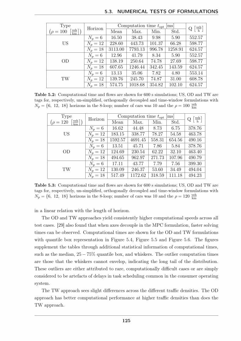
5.3. NUMERICAL TESTS OF FORMULATIONS
Type Horizon Computation time topt [ms] Q[veh
h
](ρ = 100
[vehkm
])Mean Max. Min. Std.
USNp = 6 16.50 38.43 9.98 5.90 552.57Np = 12 228.60 443.73 101.37 66.28 598.77Np = 18 3113.00 7793.13 996.78 1258.91 624.57
ODNp = 6 12.96 41.79 8.34 5.90 552.57Np = 12 138.19 250.64 74.78 27.69 598.77Np = 18 607.65 1246.44 342.45 143.59 624.57
TWNp = 6 13.13 35.06 7.82 4.80 553.14Np = 12 139.76 245.70 74.87 31.00 608.78Np = 18 574.75 1018.68 354.82 102.10 624.57
Table 5.2: Computational time and flows are shown for 600 s simulations; US, OD and TW aretags for, respectively, un-simplified, orthogonally decoupled and time-window formulations withNp = 6, 12, 18 horizons in the 8-loop; number of cars was 10 and the ρ = 100 veh
km
Type Horizon Computation time topt [ms] Q[veh
h
](ρ = 120
[vehkm
])Mean Max. Min. Std.
USNp = 6 16.62 44.48 8.73 6.75 378.76Np = 12 183.15 338.77 78.27 54.58 463.78Np = 18 1592.57 4691.45 558.31 654.56 490.16
ODNp = 6 13.51 45.71 7.86 5.84 378.76Np = 12 124.69 230.54 62.22 32.10 463.40Np = 18 494.65 962.97 271.73 107.96 490.79
TWNp = 6 17.11 43.77 7.79 7.56 399.30Np = 12 130.09 246.37 53.60 34.49 494.04Np = 18 517.49 1172.62 318.59 111.18 494.23
Table 5.3: Computational time and flows are shown for 600 s simulations; US, OD and TW aretags for, respectively, un-simplified, orthogonally decoupled and time-window formulations withNp = 6, 12, 18 horizons in the 8-loop; number of cars was 10 and the ρ = 120 veh
km
in a linear relation with the length of horizon.The OD and TW approaches yield consistently higher computational speeds across all
test cases. [29] also found that when axes decouple in the MPC formulation, faster solvingtimes can be observed. Computational times are shown for the OD and TW formulationswith quantile box representation in Figure 5.4, Figure 5.5 and Figure 5.6. The figuressupplement the tables through additional statistical information of computational times,such as the median, 25− 75% quantile box, and whiskers. The outlier computation timesare those that the whiskers cannot envelop, indicating the long tail of the distribution.These outliers are either attributed to rare, computationally difficult cases or are simplyconsidered to be artefacts of delays in task scheduling common in the consumer operatingsystem.
The TW approach sees slight differences across the different traffic densities. The ODapproach has better computational performance at higher traffic densities than does theTW approach.
125
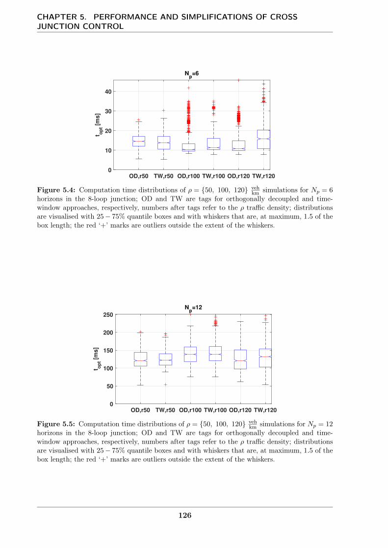
CHAPTER 5. PERFORMANCE AND SIMPLIFICATIONS OF CROSSJUNCTION CONTROL
OD,r50 TW,r50 OD,r100 TW,r100 OD,r120 TW,r1200
10
20
30
40t o
pt [
ms
]
Np=6
Figure 5.4: Computation time distributions of ρ = 50, 100, 120 vehkm simulations for Np = 6
horizons in the 8-loop junction; OD and TW are tags for orthogonally decoupled and time-window approaches, respectively, numbers after tags refer to the ρ traffic density; distributionsare visualised with 25− 75% quantile boxes and with whiskers that are, at maximum, 1.5 of thebox length; the red ‘+’ marks are outliers outside the extent of the whiskers.
OD,r50 TW,r50 OD,r100 TW,r100 OD,r120 TW,r1200
50
100
150
200
250
t op
t [m
s]
Np=12
Figure 5.5: Computation time distributions of ρ = 50, 100, 120 vehkm simulations for Np = 12
horizons in the 8-loop junction; OD and TW are tags for orthogonally decoupled and time-window approaches, respectively, numbers after tags refer to the ρ traffic density; distributionsare visualised with 25− 75% quantile boxes and with whiskers that are, at maximum, 1.5 of thebox length; the red ‘+’ marks are outliers outside the extent of the whiskers.
126
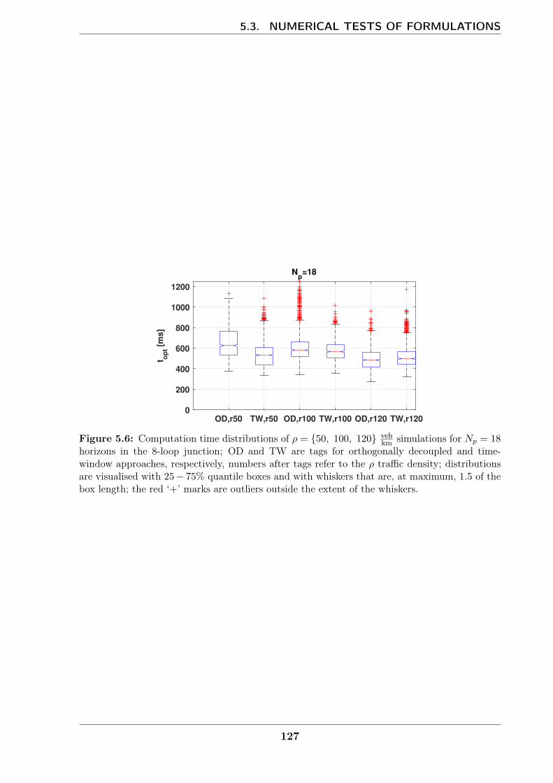
5.3. NUMERICAL TESTS OF FORMULATIONS
OD,r50 TW,r50 OD,r100 TW,r100 OD,r120 TW,r1200
200
400
600
800
1000
1200
t op
t [m
s]
Np=18
Figure 5.6: Computation time distributions of ρ = 50, 100, 120 vehkm simulations for Np = 18
horizons in the 8-loop junction; OD and TW are tags for orthogonally decoupled and time-window approaches, respectively, numbers after tags refer to the ρ traffic density; distributionsare visualised with 25− 75% quantile boxes and with whiskers that are, at maximum, 1.5 of thebox length; the red ‘+’ marks are outliers outside the extent of the whiskers.
127
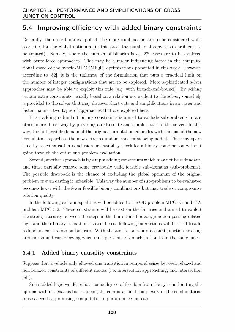
CHAPTER 5. PERFORMANCE AND SIMPLIFICATIONS OF CROSSJUNCTION CONTROL
5.4 Improving efficiency with added binary constraints
Generally, the more binaries applied, the more combination are to be considered whilesearching for the global optimum (in this case, the number of convex sub-problems tobe treated). Namely, where the number of binaries is nb, 2nb cases are to be exploredwith brute-force approaches. This may be a major influencing factor in the computa-tional speed of the hybrid-MPC (MIQP) optimisations presented in this work. However,according to [82], it is the tightness of the formulation that puts a practical limit onthe number of integer configurations that are to be explored. More sophisticated solverapproaches may be able to exploit this rule (e.g. with branch-and-bound). By addingcertain extra constraints, usually based on a relation not evident to the solver, some helpis provided to the solver that may discover short cuts and simplifications in an easier andfaster manner; two types of approaches that are explored here.
First, adding redundant binary constraints is aimed to exclude sub-problems in an-other, more direct way by providing an alternate and simpler path to the solver. In thisway, the full feasible domain of the original formulation coincides with the one of the newformulation regardless the new extra redundant constraint being added. This may sparetime by reaching earlier conclusion or feasibility check for a binary combination withoutgoing through the entire sub-problem evaluation.
Second, another approach is by simply adding constraints which may not be redundant,and thus, partially remove some previously valid feasible sub-domains (sub-problems).The possible drawback is the chance of excluding the global optimum of the originalproblem or even casting it infeasible. This way the number of sub-problems to be evaluatedbecomes fewer with the fewer feasible binary combinations but may trade or compromisesolution quality.
In the following extra inequalities will be added to the OD problem MPC 5.1 and TWproblem MPC 5.2. These constraints will be cast on the binaries and aimed to exploitthe strong causality between the steps in the finite time horizon, junction passing relatedlogic and their binary relaxation. Later the car-following interactions will be used to addredundant constraints on binaries. With the aim to take into account junction crossingarbitration and car-following when multiple vehicles do arbitration from the same lane.
5.4.1 Added binary causality constraints
Suppose that a vehicle only allowed one transition in temporal sense between relaxed andnon-relaxed constraints of different modes (i.e. intersection approaching, and intersectionleft).
Such added logic would remove some degree of freedom from the system, limiting theoptions within scenarios but reducing the computational complexity in the combinatorialsense as well as promising computational performance increase.
128
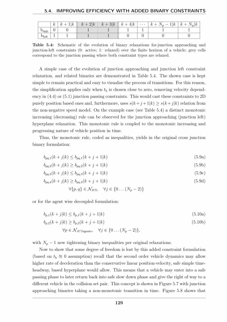
5.4. IMPROVING EFFICIENCY WITH ADDED BINARY CONSTRAINTS
k k + 1|k k + 2|k k + 3|k k + 4|k · · · k +Np − 1|k k +Np|kbapp 0 0 1 1 1 1 1 1bleft 1 1 1 1 0 0 0 0
Table 5.4: Schematic of the evolution of binary relaxations for-junction approaching andjunction-left constraints (0: active; 1: relaxed) over the finite horizon of a vehicle; grey cellscorrespond to the junction passing where both constraint types are relaxed.
A simple case of the evolution of junction approaching and junction left constraintrelaxation, and related binaries are demonstrated in Table 5.4. The shown case is keptsimple to remain practical and easy to visualise the process of transitions. For this reason,the simplification applies only when th is chosen close to zero, removing velocity depend-ency in (4.4) or (5.1) junction passing constraints. This would cast these constraints to 2Dpurely position based ones and, furthermore, uses s(k+j+1|k) ≥ s(k+j|k) relation fromthe non-negative speed model. On the example case (see Table 5.4) a distinct monotonicincreasing (decreasing) rule can be observed for the junction approaching (junction left)hyperplane relaxation. This monotonic rule is coupled to the monotonic increasing andprogressing nature of vehicle position in time.
Thus, the monotonic rule, coded as inequalities, yields in the original cross junctionbinary formulation:
bpq,1(k + j|k) ≤ bpq,1(k + j + 1|k) (5.9a)
bpq,2(k + j|k) ≥ bpq,2(k + j + 1|k) (5.9b)
bpq,3(k + j|k) ≤ bpq,3(k + j + 1|k) (5.9c)
bpq,4(k + j|k) ≥ bpq,4(k + j + 1|k) (5.9d)
∀p, q ∈ NJCI, ∀j ∈ 0 . . . (Np − 2)
or for the agent wise decoupled formulation:
bp,1(k + j|k) ≤ bp,1(k + j + 1|k) (5.10a)
bp,2(k + j|k) ≥ bp,2(k + j + 1|k) (5.10b)
∀p ∈ NJCIagents, ∀j ∈ 0 . . . (Np − 2),
with Np − 1 new tightening binary inequalities per original relaxations.Now to show that some degree of freedom is lost by this added constraint formulation
(based on th u 0 assumption) recall that the second order vehicle dynamics may allowhigher rate of deceleration than the conservative linear position-velocity, safe simple time-headway, based hyperplane would allow. This means that a vehicle may enter into a safepassing phase to later return back into safe slow down phase and give the right of way to adifferent vehicle in the collision set pair. This concept is shown in Figure 5.7 with junctionapproaching binaries taking a non-monotonic transition in time. Figure 5.8 shows that
129
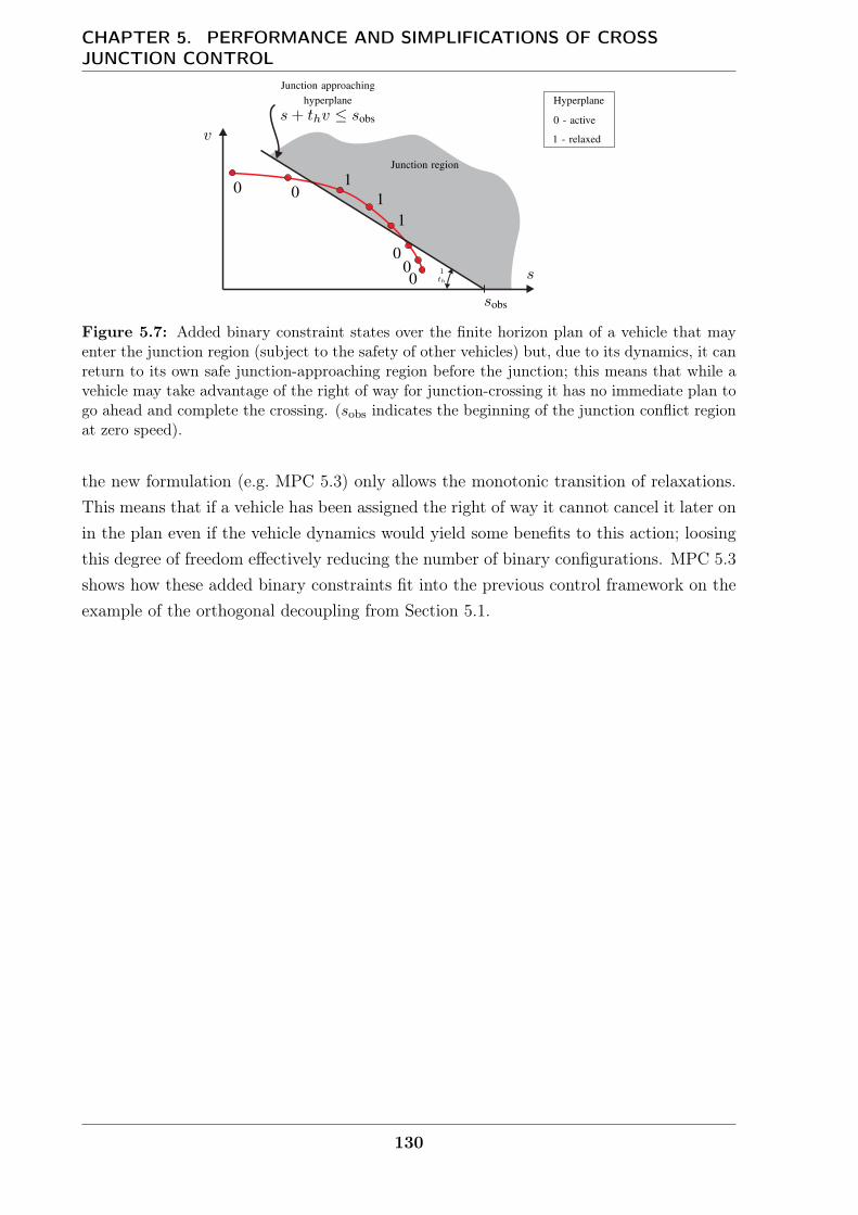
CHAPTER 5. PERFORMANCE AND SIMPLIFICATIONS OF CROSSJUNCTION CONTROL
Figure 5.7: Added binary constraint states over the finite horizon plan of a vehicle that mayenter the junction region (subject to the safety of other vehicles) but, due to its dynamics, it canreturn to its own safe junction-approaching region before the junction; this means that while avehicle may take advantage of the right of way for junction-crossing it has no immediate plan togo ahead and complete the crossing. (sobs indicates the beginning of the junction conflict regionat zero speed).
the new formulation (e.g. MPC 5.3) only allows the monotonic transition of relaxations.This means that if a vehicle has been assigned the right of way it cannot cancel it later onin the plan even if the vehicle dynamics would yield some benefits to this action; loosingthis degree of freedom effectively reducing the number of binary configurations. MPC 5.3shows how these added binary constraints fit into the previous control framework on theexample of the orthogonal decoupling from Section 5.1.
130

5.4. IMPROVING EFFICIENCY WITH ADDED BINARY CONSTRAINTS
Figure 5.8: Finite horizon plans with indicated binary states where, due to the constraintsadded, after the vehicle has relaxed its safe junction-approaching hyperplane, it may enter thejunction region (subject the safety of other vehicles) or, as shown in (a), return the set of statespreviously satisfying the junction approaching-hyperplane. However, it remains the sole holderof the right of way within the rest of the current plan, and it may only be given away oncethe vehicle leaves the junction region. In contrast, without the added constraints, the vehiclewould be able to cancel its right of way (see Figure 5.7). (b) shows a healthy crossing where thetightening may make no apparent change (sobs indicates the beginning of the junction conflictregion at zero speed).
MPC-5.3
J∗MPC-5.3 = min (4.1)
s.t. ∀j ∈ 0 . . . (Np − 1), ∀n ∈ N :
xn (k|k) = xn (k)
xn (k + j + 1|k) = A xn (k + j|k) +B un (k + j|k)
(xn, un) ∈ Xn × Un∀(p, q) ∈ NCFI :
(4.3)
∀p ∈ NJCIagents :
(5.1a)–(5.1d)
and ∀p, q ∈ NJCI :
(5.2)
and ∀p ∈ NBoxAgents :
(4.22a)–(4.22b)
and ∀p ∈ NJCIagents , ∀j ∈ 0 . . . (Np − 2) :
(5.10a)–(5.10b).
131
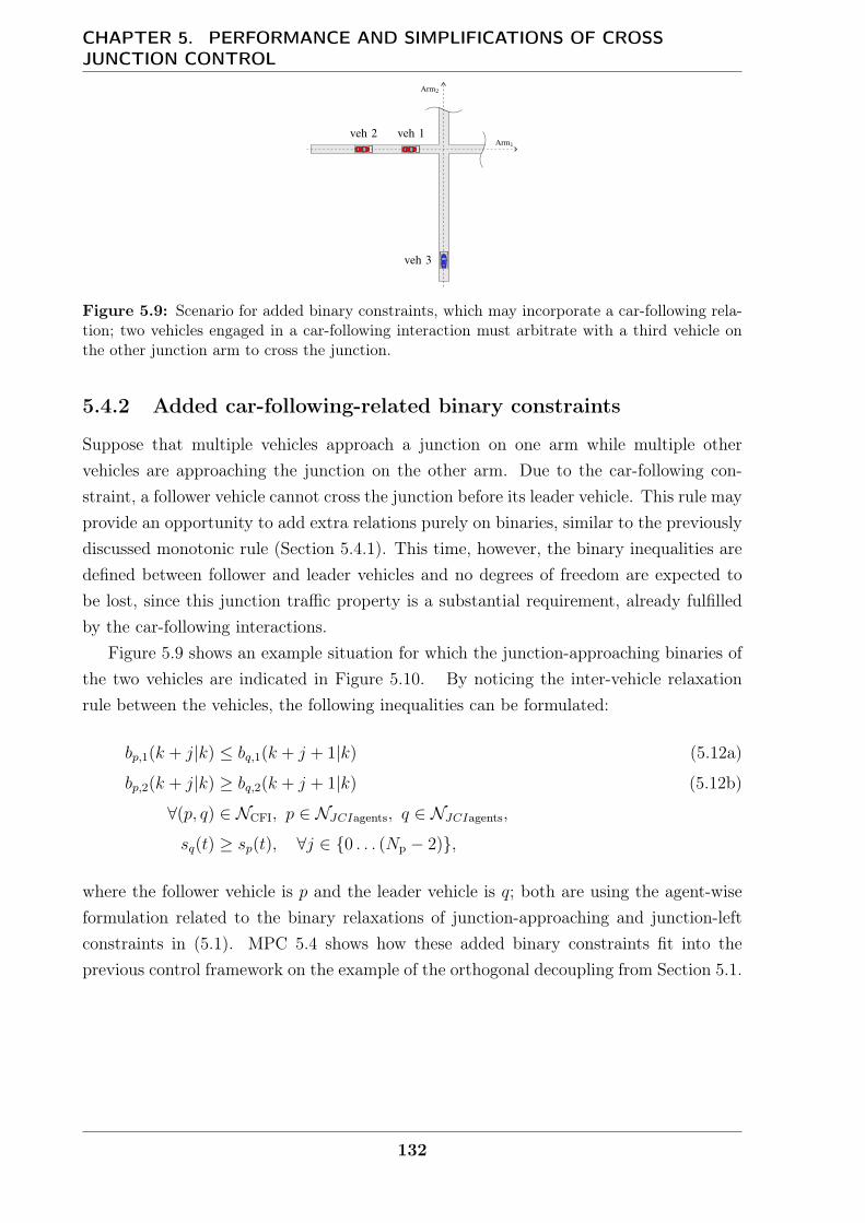
CHAPTER 5. PERFORMANCE AND SIMPLIFICATIONS OF CROSSJUNCTION CONTROL
Figure 5.9: Scenario for added binary constraints, which may incorporate a car-following rela-tion; two vehicles engaged in a car-following interaction must arbitrate with a third vehicle onthe other junction arm to cross the junction.
5.4.2 Added car-following-related binary constraints
Suppose that multiple vehicles approach a junction on one arm while multiple othervehicles are approaching the junction on the other arm. Due to the car-following con-straint, a follower vehicle cannot cross the junction before its leader vehicle. This rule mayprovide an opportunity to add extra relations purely on binaries, similar to the previouslydiscussed monotonic rule (Section 5.4.1). This time, however, the binary inequalities aredefined between follower and leader vehicles and no degrees of freedom are expected tobe lost, since this junction traffic property is a substantial requirement, already fulfilledby the car-following interactions.
Figure 5.9 shows an example situation for which the junction-approaching binaries ofthe two vehicles are indicated in Figure 5.10. By noticing the inter-vehicle relaxationrule between the vehicles, the following inequalities can be formulated:
bp,1(k + j|k) ≤ bq,1(k + j + 1|k) (5.12a)
bp,2(k + j|k) ≥ bq,2(k + j + 1|k) (5.12b)
∀(p, q) ∈ NCFI, p ∈ NJCIagents, q ∈ NJCIagents,
sq(t) ≥ sp(t), ∀j ∈ 0 . . . (Np − 2),
where the follower vehicle is p and the leader vehicle is q; both are using the agent-wiseformulation related to the binary relaxations of junction-approaching and junction-leftconstraints in (5.1). MPC 5.4 shows how these added binary constraints fit into theprevious control framework on the example of the orthogonal decoupling from Section 5.1.
132
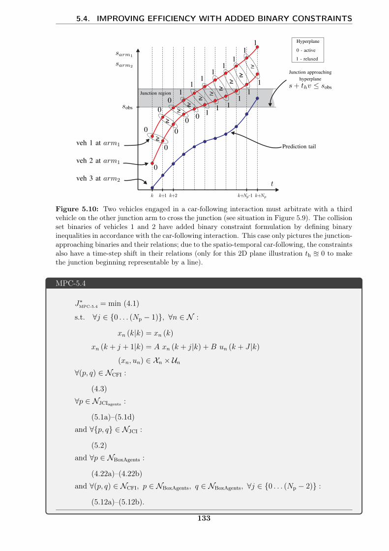
5.4. IMPROVING EFFICIENCY WITH ADDED BINARY CONSTRAINTS
Figure 5.10: Two vehicles engaged in a car-following interaction must arbitrate with a thirdvehicle on the other junction arm to cross the junction (see situation in Figure 5.9). The collisionset binaries of vehicles 1 and 2 have added binary constraint formulation by defining binaryinequalities in accordance with the car-following interaction. This case only pictures the junction-approaching binaries and their relations; due to the spatio-temporal car-following, the constraintsalso have a time-step shift in their relations (only for this 2D plane illustration th u 0 to makethe junction beginning representable by a line).
MPC-5.4
J∗MPC-5.4 = min (4.1)
s.t. ∀j ∈ 0 . . . (Np − 1), ∀n ∈ N :
xn (k|k) = xn (k)
xn (k + j + 1|k) = A xn (k + j|k) +B un (k + J |k)
(xn, un) ∈ Xn × Un∀(p, q) ∈ NCFI :
(4.3)
∀p ∈ NJCIagents :
(5.1a)–(5.1d)
and ∀p, q ∈ NJCI :
(5.2)
and ∀p ∈ NBoxAgents :
(4.22a)–(4.22b)
and ∀(p, q) ∈ NCFI, p ∈ NBoxAgents, q ∈ NBoxAgents, ∀j ∈ 0 . . . (Np − 2) :
(5.12a)–(5.12b).
133
CHAPTER 5. PERFORMANCE AND SIMPLIFICATIONS OF CROSSJUNCTION CONTROL
5.5 Numerical tests with added binary constraints
The added binary constraint cases are shown only for the OD and TW formulations,as they have better computational performances than the US formulation, as shown inSection 5.3. Furthermore, only the horizon lengths of Np = 6 and Np = 12 are consideredbecause the data in Section 5.3 revealed that Np = 18 would yield considerably longercomputational times than the control time step δt = 0.5 s for N = 10 vehicles, whichwould not be appropriate for real-time control in this case. The test cases are the baseproblem formulations without the added binary constraints, the two single cases shownin Section 5.4.1 and Section 5.4.2, and the test cases in which both types of these binaryconstraints are added.
Appendix A presents the computational time and average flow results collected inTable A.1, Table A.2 and Table A.3. The results indicate that, in most cases, the singe-agent related added binary constraints from Section 5.4.1 resulted in lower flows due tothe removed degree of freedom. There was a slight improvement in a few cases but nonethat was consistent for all computation times. The car-following related added binaryconstraint method shown in Section 5.4.2 did not result in any significantly differentflows than the cases without it; however, it increased the overhead and calculation timebecause the increased number of constraints in the optimisation. In fact, the added binaryconstraints of this kind are already implied by the car-following constraints indirectly butthe solver (Gurobi) has been able to consider this indirect link in its branch-and-boundalgorithm, solving the mixed-integer program. This means that, since the complexityremained the same but computation time and problem size increased, there were onlynegative effects for this approach.
A similar idea using car-following orders to enhance the control performance wasmentioned in [1]; however, in contrast to the theorised computational benefits there, thedata suggests that the implementation analysed here yields increased computational timeand problem size.
The last case is that which employs both added binary constraint formulations to-gether, which inherits both the lower flow measure from the reduced degree of freedomand the overhead time from the car-following-related added binary constraints. This caseconsistently reached solution times in the range of computation times measured for thecases that only applied one of the added binary constraint techniques.
134

5.6. DECENTRALISATION
5.6 Decentralisation
In this section, the predictive control will be formulated for smaller but connected sub-problems, exchanging calculated plans between agents in sequential order. Sequentialdecentralisation was discussed for a predictive multi-agent system in [62]. Centralisedapproaches scale poorly and hard to tackle above a certain size; decentralisation is an at-tractive way to fix scaling issues of a problem especially for large systems [49]. Scattolini[69] surveys the distributed MPC formulations and notes that vehicle-related problemsare usually coupled through obstacle avoidance constraints and the sub-systems are de-coupled in dynamics. Dunbar and Murray [23] show an early work for stabilisation ofmultiple-vehicle formation, where sub-systems are coupled through the cost. In [76], theagents are coupled and interacting via constraints in a tube-MPC approach. This accom-modates agents with added uncertainty to safely travel in their tubes and uses sequentialreplanning, through which agents update one plan at a time. In the case of road vehiclecontrol, Debada et al. [21] demonstrate a cooperative framework for sharing differentlevels of information between vehicles, including future MPC plans to improve the trafficthroughput in junctions and roundabouts.
Shi et al. [71] illustrate a decentralised solution framework to conform with MPClike behaviour, ensuring a rear-end-collision-free system while new vehicles on arrival areadded to the problem.
The rear-end-collision-free property in the decentralised formulation shown here ishandled by the simple time-headway safety constraints and the upstream sequencingwhen hard prediction tails are shared.
5.6.1 Problem formulation
In this problem, the vehicles are only able to gain information about their surroundingsfrom within a given vicinity. For example, assume that a vehicle in question (ego vehicle)is moving into a cross junction (see Figure 5.11). The detection area within which the egovehicle is able to gather information is a square-shaped area centred on the front of thevehicle box extending in all direction with the length of range lR (see Figure 5.11). Notethat this is the detection area where the range on the 2D plane is calculated in an l∞-normsense (the range in an l2-norm sense would be a circular area). From the viewpoint of theego vehicle n, vehicles in this detection area are elements of the in-range set NinR(n).
NinR(n) =
p ∈ N |
∣∣∣∣∣[xp(k)
yp(k)
]−
[xn(k)
yn(k)
]∣∣∣∣∣l1
≤ lR
, (5.14)
where the 2D Cartesian coordinates are calculated from the map (2.2) or, alternatively,from the 1D position in (2.3).
135
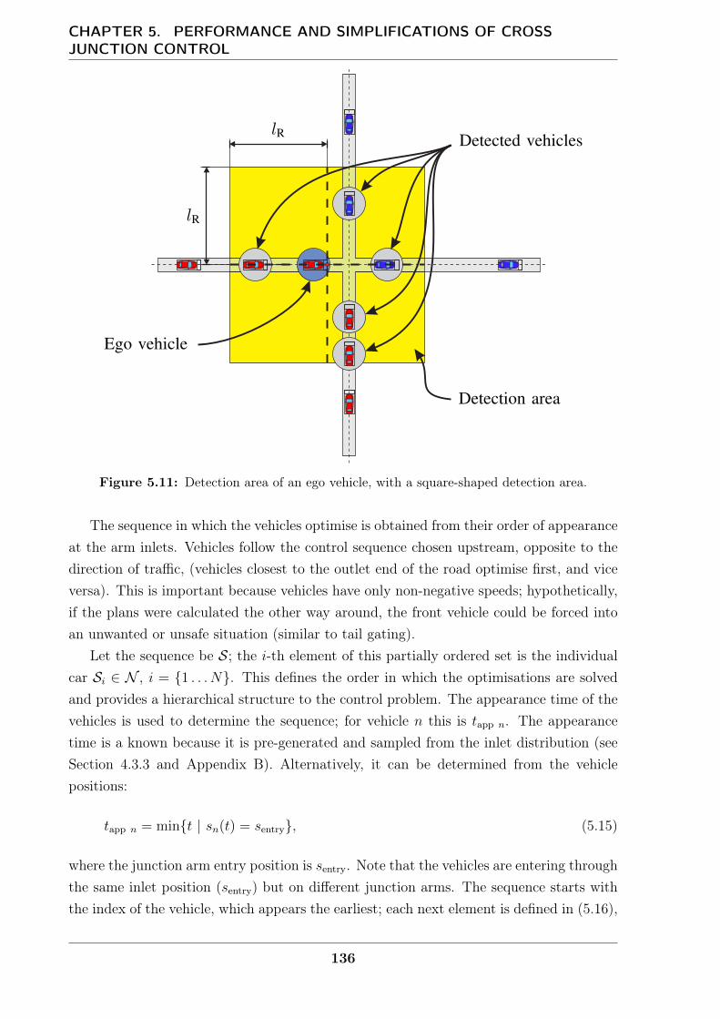
CHAPTER 5. PERFORMANCE AND SIMPLIFICATIONS OF CROSSJUNCTION CONTROL
Figure 5.11: Detection area of an ego vehicle, with a square-shaped detection area.
The sequence in which the vehicles optimise is obtained from their order of appearanceat the arm inlets. Vehicles follow the control sequence chosen upstream, opposite to thedirection of traffic, (vehicles closest to the outlet end of the road optimise first, and viceversa). This is important because vehicles have only non-negative speeds; hypothetically,if the plans were calculated the other way around, the front vehicle could be forced intoan unwanted or unsafe situation (similar to tail gating).
Let the sequence be S; the i-th element of this partially ordered set is the individualcar Si ∈ N , i = 1 . . . N. This defines the order in which the optimisations are solvedand provides a hierarchical structure to the control problem. The appearance time of thevehicles is used to determine the sequence; for vehicle n this is tapp n. The appearancetime is a known because it is pre-generated and sampled from the inlet distribution (seeSection 4.3.3 and Appendix B). Alternatively, it can be determined from the vehiclepositions:
tapp n = mint | sn(t) = sentry, (5.15)
where the junction arm entry position is sentry. Note that the vehicles are entering throughthe same inlet position (sentry) but on different junction arms. The sequence starts withthe index of the vehicle, which appears the earliest; each next element is defined in (5.16),
136
5.6. DECENTRALISATION
Algorithm 1 Vehicle controlObtain vehicle measurements xn(k), ∀n ∈ NInitialise sequence counter i = 1for n ∈ Si doReceive broadcasted solutions in range, x∗p, u∗p, ∀p ∈ (NinR(n) ∩NTx)Solve optimisation (e.g. MPC 5.5) with vehicles NinR(n)Transmit solution x∗n, u∗n in effective radiusIncrement sequence counter i = i+ 1
end forreturn u∗n(k|k), ∀n ∈ N to simulation engine
as follows:
S1 = arg minn
tapp n, (5.16a)
tapp n=Si ≤ tapp n=Si+1, i ∈ 1 . . . (N − 1), (5.16b)
which makes S a partially ordered set that orders vehicles in an upstream sequence ontheir respective road.
The vehicles that already optimised (in the current time step) broadcast without delaytheir own trajectory choices over their finite horizon x∗p, u∗p, p ∈ NTx(k), where the set ofvehicle indices that already transmitted their results at k control period is NTx(k). Thenext vehicle to optimise with index n is able to receive broadcast results of other vehiclesand fix these prediction tails in its own optimisation if the transmissions were in range,∀p ∈ (NinR(n) ∩ NTx). When both prediction tails of a pair of vehicles to be consideredin an optimisation are fixed, the interaction constraints between them are removed fromthis optimisation because they are already satisfied.
Vehicle interactions within range of and with respect to the individual ego vehicle n areformulated with the help of the set ‘vehicles in range’ NinR(n), namely NCFI(n), NJCI(n),NJCIagents(n) and NBoxAgents(n); these sets available for the ego vehicle, for simplicity, areobtained from the global sets in the simulation by considering the in-range condition; forexample:
NCFI(n) = (p, q) ∈ NCFI | p ∈ NinR(n), q ∈ NinR(n). (5.17)
Following the above logic, NJCI(n) can be generated while NJCIagents(n) represents the setof unique vehicle indices inside NJCI(n).
The structure of the MPC is detailed for the decentralisation framework in MPC 5.5 forego vehicle n, the original formulation was based on the orthogonal decoupling example.
Finally, Algorithm 1 shows the vehicle control at k control time step with the sequentialoptimisation.
137
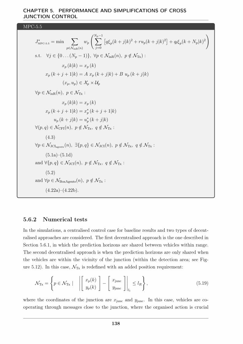
CHAPTER 5. PERFORMANCE AND SIMPLIFICATIONS OF CROSSJUNCTION CONTROL
MPC-5.5
J∗MPC-5.5 = min∑
p∈NinR(n)
wp
(Np−1∑j=0
[qξp(k + j|k)2 + rup(k + j|k)2
]+ qfξp(k +Np|k)2
)s.t. ∀j ∈ 0 . . . (Np − 1), ∀p ∈ NinR(n), p /∈ NTx) :
xp (k|k) = xp (k)
xp (k + j + 1|k) = A xp (k + j|k) +B up (k + j|k)
(xp, up) ∈ Xp × Up
∀p ∈ NinR(n), p ∈ NTx :
xp (k|k) = xp (k)
xp (k + j + 1|k) = x∗p (k + j + 1|k)
up (k + j|k) = u∗p (k + j|k)
∀(p, q) ∈ NCFI(n), p /∈ NTx, q /∈ NTx :
(4.3)
∀p ∈ NJCIagents(n), ∃p, q ∈ NJCI(n), p /∈ NTx, q /∈ NTx :
(5.1a)–(5.1d)
and ∀p, q ∈ NJCI(n), p /∈ NTx, q /∈ NTx :
(5.2)
and ∀p ∈ NBoxAgents(n), p /∈ NTx :
(4.22a)–(4.22b).
5.6.2 Numerical tests
In the simulations, a centralised control case for baseline results and two types of decent-ralised approaches are considered. The first decentralised approach is the one described inSection 5.6.1, in which the prediction horizons are shared between vehicles within range.The second decentralised approach is when the prediction horizons are only shared whenthe vehicles are within the vicinity of the junction (within the detection area; see Fig-ure 5.12). In this case, NTx is redefined with an added position requirement:
NTx =
p ∈ NTx |
∣∣∣∣∣[xp(k)
yp(k)
]−
[xjunc
yjunc
]∣∣∣∣∣l1
≤ lR
, (5.19)
where the coordinates of the junction are xjunc and yjunc. In this case, vehicles are co-operating through messages close to the junction, where the organised action is crucial
138
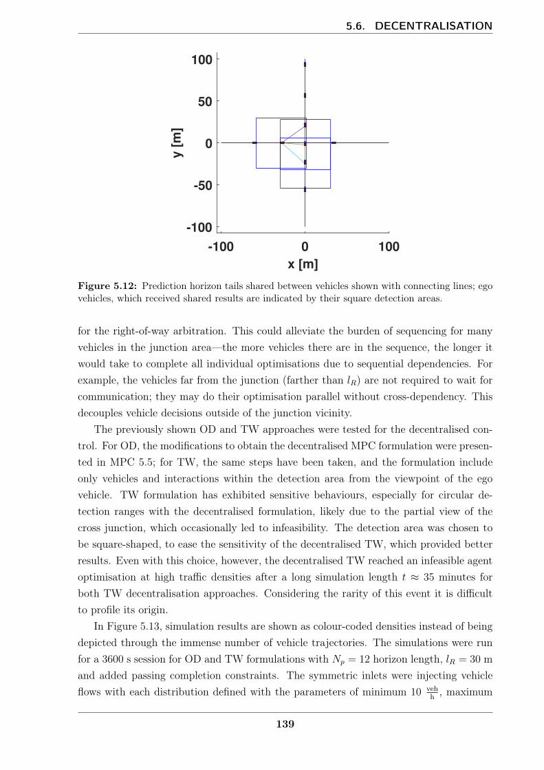
5.6. DECENTRALISATION
-100 0 100
x [m]
-100
-50
0
50
100
y [
m]
Figure 5.12: Prediction horizon tails shared between vehicles shown with connecting lines; egovehicles, which received shared results are indicated by their square detection areas.
for the right-of-way arbitration. This could alleviate the burden of sequencing for manyvehicles in the junction area—the more vehicles there are in the sequence, the longer itwould take to complete all individual optimisations due to sequential dependencies. Forexample, the vehicles far from the junction (farther than lR) are not required to wait forcommunication; they may do their optimisation parallel without cross-dependency. Thisdecouples vehicle decisions outside of the junction vicinity.
The previously shown OD and TW approaches were tested for the decentralised con-trol. For OD, the modifications to obtain the decentralised MPC formulation were presen-ted in MPC 5.5; for TW, the same steps have been taken, and the formulation includeonly vehicles and interactions within the detection area from the viewpoint of the egovehicle. TW formulation has exhibited sensitive behaviours, especially for circular de-tection ranges with the decentralised formulation, likely due to the partial view of thecross junction, which occasionally led to infeasibility. The detection area was chosen tobe square-shaped, to ease the sensitivity of the decentralised TW, which provided betterresults. Even with this choice, however, the decentralised TW reached an infeasible agentoptimisation at high traffic densities after a long simulation length t ≈ 35 minutes forboth TW decentralisation approaches. Considering the rarity of this event it is difficultto profile its origin.
In Figure 5.13, simulation results are shown as colour-coded densities instead of beingdepicted through the immense number of vehicle trajectories. The simulations were runfor a 3600 s session for OD and TW formulations with Np = 12 horizon length, lR = 30 mand added passing completion constraints. The symmetric inlets were injecting vehicleflows with each distribution defined with the parameters of minimum 10 veh
h , maximum
139
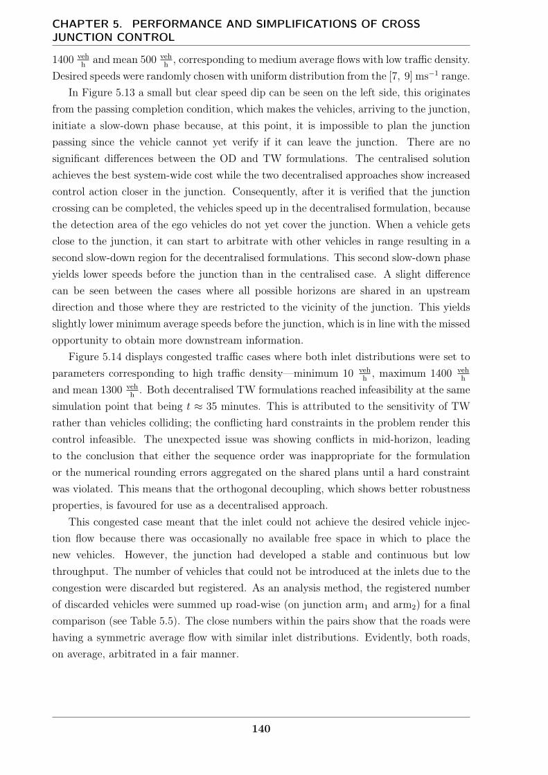
CHAPTER 5. PERFORMANCE AND SIMPLIFICATIONS OF CROSSJUNCTION CONTROL
1400 vehh and mean 500 veh
h , corresponding to medium average flows with low traffic density.Desired speeds were randomly chosen with uniform distribution from the [7, 9] ms−1 range.
In Figure 5.13 a small but clear speed dip can be seen on the left side, this originatesfrom the passing completion condition, which makes the vehicles, arriving to the junction,initiate a slow-down phase because, at this point, it is impossible to plan the junctionpassing since the vehicle cannot yet verify if it can leave the junction. There are nosignificant differences between the OD and TW formulations. The centralised solutionachieves the best system-wide cost while the two decentralised approaches show increasedcontrol action closer in the junction. Consequently, after it is verified that the junctioncrossing can be completed, the vehicles speed up in the decentralised formulation, becausethe detection area of the ego vehicles do not yet cover the junction. When a vehicle getsclose to the junction, it can start to arbitrate with other vehicles in range resulting in asecond slow-down region for the decentralised formulations. This second slow-down phaseyields lower speeds before the junction than in the centralised case. A slight differencecan be seen between the cases where all possible horizons are shared in an upstreamdirection and those where they are restricted to the vicinity of the junction. This yieldsslightly lower minimum average speeds before the junction, which is in line with the missedopportunity to obtain more downstream information.
Figure 5.14 displays congested traffic cases where both inlet distributions were set toparameters corresponding to high traffic density—minimum 10 veh
h , maximum 1400 vehh
and mean 1300 vehh . Both decentralised TW formulations reached infeasibility at the same
simulation point that being t ≈ 35 minutes. This is attributed to the sensitivity of TWrather than vehicles colliding; the conflicting hard constraints in the problem render thiscontrol infeasible. The unexpected issue was showing conflicts in mid-horizon, leadingto the conclusion that either the sequence order was inappropriate for the formulationor the numerical rounding errors aggregated on the shared plans until a hard constraintwas violated. This means that the orthogonal decoupling, which shows better robustnessproperties, is favoured for use as a decentralised approach.
This congested case meant that the inlet could not achieve the desired vehicle injec-tion flow because there was occasionally no available free space in which to place thenew vehicles. However, the junction had developed a stable and continuous but lowthroughput. The number of vehicles that could not be introduced at the inlets due to thecongestion were discarded but registered. As an analysis method, the registered numberof discarded vehicles were summed up road-wise (on junction arm1 and arm2) for a finalcomparison (see Table 5.5). The close numbers within the pairs show that the roads werehaving a symmetric average flow with similar inlet distributions. Evidently, both roads,on average, arbitrated in a fair manner.
140
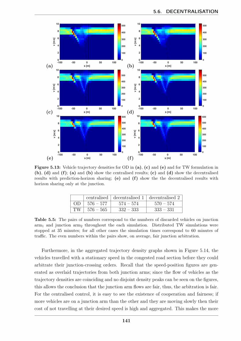
5.6. DECENTRALISATION
(a)-100 -50 0 50 100
s [m]
0
2
4
6
8
10
v [
m/s
]
0
100
200
300
400
500
(b)-100 -50 0 50 100
s [m]
0
2
4
6
8
10
v [
m/s
]
0
100
200
300
400
500
(c)-100 -50 0 50 100
s [m]
0
2
4
6
8
10
v [
m/s
]
0
100
200
300
400
500
(d)-100 -50 0 50 100
s [m]
0
2
4
6
8
10
v [
m/s
]
0
100
200
300
400
500
(e)-100 -50 0 50 100
s [m]
0
2
4
6
8
10
v [
m/s
]
0
100
200
300
400
500
600
(f)-100 -50 0 50 100
s [m]
0
2
4
6
8
10
v [
m/s
]
0
100
200
300
400
500
600
Figure 5.13: Vehicle trajectory densities for OD in (a), (c) and (e) and for TW formulation in(b), (d) and (f); (a) and (b) show the centralised results; (c) and (d) show the decentralisedresults with prediction-horizon sharing; (e) and (f) show the the decentralised results withhorizon sharing only at the junction.
centralised decentralised 1 decentralised 2OD 576 – 577 574 – 574 570 – 574TW 576 – 565 332 – 333 333 – 331
Table 5.5: The pairs of numbers correspond to the numbers of discarded vehicles on junctionarm1 and junction arm2 throughout the each simulation. Distributed TW simulations werestopped at 35 minutes; for all other cases the simulation times correspond to 60 minutes oftraffic. The even numbers within the pairs show, on average, fair junction arbitration.
Furthermore, in the aggregated trajectory density graphs shown in Figure 5.14, thevehicles travelled with a stationary speed in the congested road section before they couldarbitrate their junction-crossing orders. Recall that the speed-position figures are gen-erated as overlaid trajectories from both junction arms; since the flow of vehicles as thetrajectory densities are coinciding and no disjoint density peaks can be seen on the figures,this allows the conclusion that the junction arm flows are fair, thus, the arbitration is fair.For the centralised control, it is easy to see the existence of cooperation and fairness; ifmore vehicles are on a junction arm than the other and they are moving slowly then theircost of not travelling at their desired speed is high and aggregated. This makes the more
141

CHAPTER 5. PERFORMANCE AND SIMPLIFICATIONS OF CROSSJUNCTION CONTROL
(a)-100 -50 0 50 100
s [m]
0
2
4
6
8
10
v [
m/s
]
0
200
400
600
800
1000
1200
(b)-100 -50 0 50 100
s [m]
0
2
4
6
8
10
v [
m/s
]
0
200
400
600
800
1000
1200
(c)-100 -50 0 50 100
s [m]
0
2
4
6
8
10
v [
m/s
]
0
200
400
600
800
1000
1200
(d)-100 -50 0 50 100
s [m]
0
2
4
6
8
10
v [
m/s
]
0
200
400
600
(e)-100 -50 0 50 100
s [m]
0
2
4
6
8
10
v [
m/s
]
0
200
400
600
800
1000
1200
(f)-100 -50 0 50 100
s [m]
0
2
4
6
8
10
v [
m/s
]
0
200
400
600
Figure 5.14: Congested vehicle trajectory densities for OD in (a), (c) and (e) and for TWformulation in (b), (d) and (f); (a) and (b) show the centralised results; (c) and (d) show thedecentralised results with prediction horizon sharing; (e) and (f) show the decentralised resultswith horizon sharing only at the junction; in (d) and (f) the results are only until the distributedTW formulations encountered an infeasible optimisation at t ≈ 35 minutes.
fortunate higher-flow traffic be considerate of those on the other junction arm and grantthe congested arm the right of way.
Imagine the situation of ego vehicles travelling on congested junction arms in thedecentralised framework. The detection area of vehicles spans all around them even behindof them (recall the shape of the detection area, Figure 5.12). It may be argued that there isno specific reason to include vehicles behind the ego vehicle in the optimisation; however,this allows a cost pressure to be generated on the vehicles. As with the centralised casewhen the flow on one junction arm suffers more than that on the other, the arbitrationfollows cooperative fairness proven also by the balanced drop numbers in Table 5.5. Thisfairness element makes the method more like a locally centralised control scheme whilestill remaining decentralised overall.
142
5.7. SUMMARY
5.7 Summary
This chapter discussed performance enhancements and improved scaling formulationsbased on agent-wise hyperplanes exploiting the structure of the cross junction obstacleshapes in the collision sets. The removal of redundant hyperplanes and their binary vari-ables allowed for the achievement of higher optimisation speeds. With using the sameconsiderations, a time-window allocation approach was shown to operate with just a singleconnecting separating-hyperplane binary relation. Two added binary causality constraintapproaches were shown, in which reducing the degree of freedom led to slightly lowercomputation times at the cost of lower flows in dense traffic. Furthermore, by adding bin-ary constraints, that incorporate car-following relations into junction arbitration revealedno benefit and only increased the overhead time. Finally, the decentralised formulationproved the emergence of cooperative fairness in the cross junction arbitration and trafficflows with sequentially shared MPC predictions between vehicles. In this approach, or-thogonal decoupled decentralisation was found to cope well in the simulations.
143

144

6Concluding remarks
In Chapter 2, a mixed-integer MPC relaxation formulation was developed for central-ised autonomous driving with positive control-invariant safety constraints based on thetime-headway parameter for Y-junction merging. Corner-cutting prevention was addedto account for the worst-case leader-vehicle dynamics, making no optimistic assumptionsabout leader dynamics for one control time step. The recursive feasibility of the MPCalgorithm was theoretically, and later numerically, verified. Decision graphs were createdshowing the dependency of decisions on inter-vehicle gaps and relative priority weight-ing. These vehicle-order decisions were shown to be dependent on the distance from themerging point and, after a limit distance, they settled to a periodic relation with un-derlying phase property. In line with expectations, numerical examples with multiplevehicles showed that changing relative vehicle weightings affected the merging order, andthe control framework accomplished vehicle cooperation.
Chapter 3 inspected the cost function of the control method, where the stability proofcould be shown for an l1-norm terminal-cost-based objective function. Furthermore, thel1-norm-based formulation has a soft behaviour that can be tuned to coincide with the‘running-cost’ formulation with hard terminal set constraints of simple time-headwaysafety, also providing the stability proof for the later formulation. This is due to the‘running-cost’ being one of the three cases from the decomposed l1-norm form. Further-more, the tuning and choice of the simple time headway give the vehicle trajectories adistinct near-obstacle deceleration that was found to safeguard obstacle avoidance forvery short horizon controls and give a softer slow-down-approach phase for longer hori-zons. To promote earlier merging actions than what the horizon length would dictate andto smoothly comb vehicles from the merging junction arms, a soft pre-merging heuristicwas formulated to heuristically minimise future vehicle-state conflicts through added costterms. Additionally, minimal and maximum speed bound regions were formulated withthe safe time headway and corner-cutting prevention using the mixed-integer formulation.
Cross-junction multi-agent simulations were tackled in Chapter 4, which largely ad-
145
CHAPTER 6. CONCLUDING REMARKS
dressed the numerical considerations for and aspects of the problems. Three policieswere shown: baseline, FCFS and soft pre-avoidance. The baseline policy has the advant-age of full adaptability in vehicle-order changes while, in contrast, FCFS used pre-fixedvehicle-order heuristics, allowing lower computational cost but less adaptability. The softpre-avoidance policy showed increased control actions before getting near the junctionand less intense vehicle interactions near the junction region with, on average, higherpossible crossing speeds achievable through the junction. To avoid potential junction-blocking configurations, which could result in a deadlock situation, box-junction relatedconstraints were formulated to prevent vehicles from starting their crossing manoeuvre ifthey are unable to complete it within their finite horizon plan.
Chapter 5 first inspected a performance increase stemming from the removal of mul-tiple definitions of redundant obstacle constraints. This is because the structure of thecross-junction problem allows for simplifications in the general case with orthogonal de-coupling between vehicles. Moreover, using the same hyperplanes, a time-window re-source allocation policy was formulated with regard to the previous considerations forthe problem structure. Two redundant binary constraint techniques were added. Oneremoved some degrees-of-freedom using problem causality and, thus, slightly loweredcomputational cost (but in some cases also decreased the traffic flow). The other usedcar-following considerations in junction-crossing interactions; this failed to give any prac-tical performance increase, adding only overhead to the problem. Finally, decentralisedcontrol approaches were shown, in which every vehicle has a restricted field of perceptionand range of communication. Vehicles were able to maintain safe junction crossings withthe orthogonal-decoupling formulation but failed to do so in a rare event employing time-window formulation. The key element is that, before committing to cross the junction,vehicles must agree on the right-of-way by sharing sequentially their own and consideringreceived predicted plans.
6.1 Future works
Future works may use the proposed mixed-integer MPC framework for high-quality pre-dictive vehicle control even in real autonomous driving cases by extending the formulationwith robust control tools to guard against uncertainties and cast the problem robustlyfeasible. An application of the control to real-world cases may require additional elementsof efficient relaxations [38] and highly tailored MPC algorithms [81] that exploit problemstructure, warm start and early termination. Furthermore, good heuristics can primethe branch-and-bound search, increasing computation speed through techniques such asshared (networked) perception and deep learning.
The framework introduced in this thesis is concerned with the atomic junction blocks.In real-world structures, several of these atomic blocks (e.g. mergings, crossings, and
146
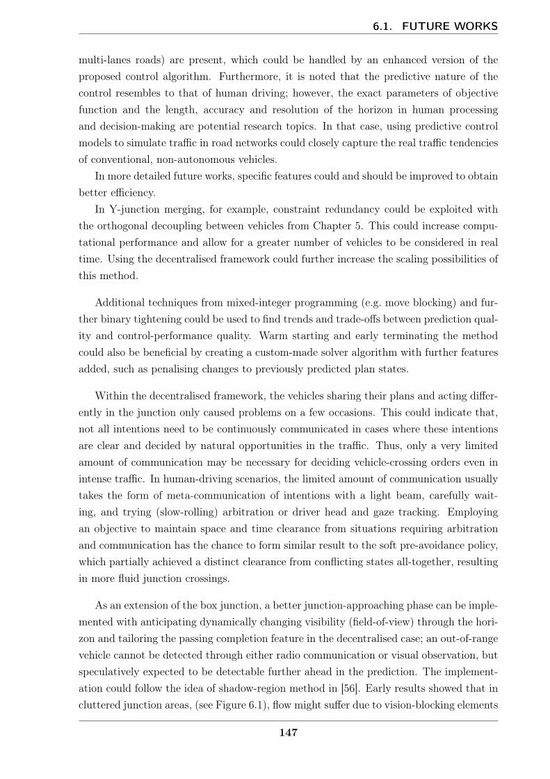
6.1. FUTURE WORKS
multi-lanes roads) are present, which could be handled by an enhanced version of theproposed control algorithm. Furthermore, it is noted that the predictive nature of thecontrol resembles to that of human driving; however, the exact parameters of objectivefunction and the length, accuracy and resolution of the horizon in human processingand decision-making are potential research topics. In that case, using predictive controlmodels to simulate traffic in road networks could closely capture the real traffic tendenciesof conventional, non-autonomous vehicles.
In more detailed future works, specific features could and should be improved to obtainbetter efficiency.
In Y-junction merging, for example, constraint redundancy could be exploited withthe orthogonal decoupling between vehicles from Chapter 5. This could increase compu-tational performance and allow for a greater number of vehicles to be considered in realtime. Using the decentralised framework could further increase the scaling possibilities ofthis method.
Additional techniques from mixed-integer programming (e.g. move blocking) and fur-ther binary tightening could be used to find trends and trade-offs between prediction qual-ity and control-performance quality. Warm starting and early terminating the methodcould also be beneficial by creating a custom-made solver algorithm with further featuresadded, such as penalising changes to previously predicted plan states.
Within the decentralised framework, the vehicles sharing their plans and acting differ-ently in the junction only caused problems on a few occasions. This could indicate that,not all intentions need to be continuously communicated in cases where these intentionsare clear and decided by natural opportunities in the traffic. Thus, only a very limitedamount of communication may be necessary for deciding vehicle-crossing orders even inintense traffic. In human-driving scenarios, the limited amount of communication usuallytakes the form of meta-communication of intentions with a light beam, carefully wait-ing, and trying (slow-rolling) arbitration or driver head and gaze tracking. Employingan objective to maintain space and time clearance from situations requiring arbitrationand communication has the chance to form similar result to the soft pre-avoidance policy,which partially achieved a distinct clearance from conflicting states all-together, resultingin more fluid junction crossings.
As an extension of the box junction, a better junction-approaching phase can be imple-mented with anticipating dynamically changing visibility (field-of-view) through the hori-zon and tailoring the passing completion feature in the decentralised case; an out-of-rangevehicle cannot be detected through either radio communication or visual observation, butspeculatively expected to be detectable further ahead in the prediction. The implement-ation could follow the idea of shadow-region method in [56]. Early results showed that incluttered junction areas, (see Figure 6.1), flow might suffer due to vision-blocking elements
147
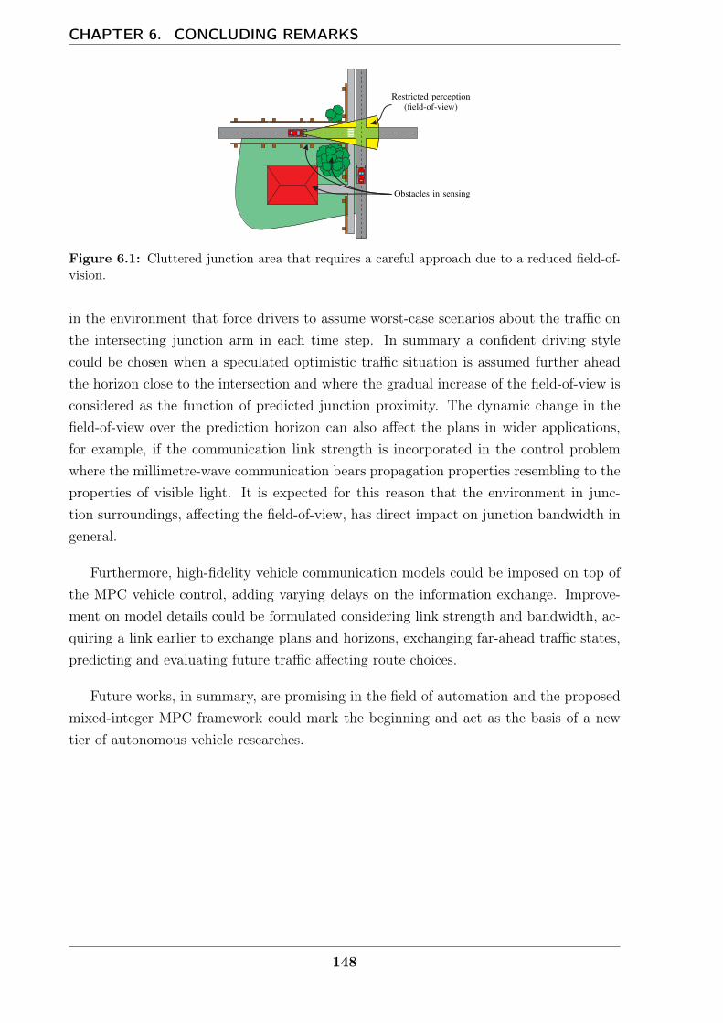
CHAPTER 6. CONCLUDING REMARKS
Figure 6.1: Cluttered junction area that requires a careful approach due to a reduced field-of-vision.
in the environment that force drivers to assume worst-case scenarios about the traffic onthe intersecting junction arm in each time step. In summary a confident driving stylecould be chosen when a speculated optimistic traffic situation is assumed further aheadthe horizon close to the intersection and where the gradual increase of the field-of-view isconsidered as the function of predicted junction proximity. The dynamic change in thefield-of-view over the prediction horizon can also affect the plans in wider applications,for example, if the communication link strength is incorporated in the control problemwhere the millimetre-wave communication bears propagation properties resembling to theproperties of visible light. It is expected for this reason that the environment in junc-tion surroundings, affecting the field-of-view, has direct impact on junction bandwidth ingeneral.
Furthermore, high-fidelity vehicle communication models could be imposed on top ofthe MPC vehicle control, adding varying delays on the information exchange. Improve-ment on model details could be formulated considering link strength and bandwidth, ac-quiring a link earlier to exchange plans and horizons, exchanging far-ahead traffic states,predicting and evaluating future traffic affecting route choices.
Future works, in summary, are promising in the field of automation and the proposedmixed-integer MPC framework could mark the beginning and act as the basis of a newtier of autonomous vehicle researches.
148
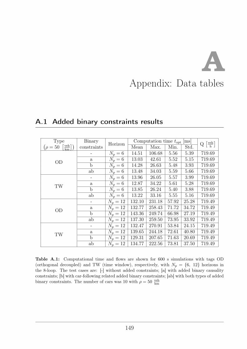
AAppendix: Data tables
A.1 Added binary constraints results
Type Binary Horizon Computation time topt [ms] Q[veh
h
](ρ = 50
[vehkm
])constraints Mean Max. Min. Std.
OD
- Np = 6 14.51 106.68 5.56 5.39 719.69a Np = 6 13.03 42.61 5.52 5.15 719.69b Np = 6 14.28 26.63 5.48 3.93 719.69ab Np = 6 13.48 34.03 5.59 5.66 719.69
TW
- Np = 6 13.96 26.05 5.57 3.99 719.69a Np = 6 12.87 34.22 5.61 5.28 719.69b Np = 6 13.85 26.24 5.40 3.88 719.69ab Np = 6 13.22 33.16 5.55 5.16 719.69
OD
- Np = 12 132.10 231.18 57.92 25.28 719.49a Np = 12 132.77 258.43 71.72 34.72 719.49b Np = 12 143.36 249.74 66.98 27.19 719.49ab Np = 12 137.30 259.50 73.95 33.92 719.49
TW
- Np = 12 132.47 270.91 53.84 24.15 719.49a Np = 12 139.65 244.18 72.61 40.80 719.49b Np = 12 129.31 207.65 71.63 20.69 719.49ab Np = 12 134.77 222.56 73.81 37.50 719.49
Table A.1: Computational time and flows are shown for 600 s simulations with tags OD(orthogonal decoupled) and TW (time window), respectively, with Np = 6, 12 horizons inthe 8-loop. The test cases are: [-] without added constraints; [a] with added binary causalityconstraints; [b] with car-following related added binary constraints; [ab] with both types of addedbinary constraints. The number of cars was 10 with ρ = 50 veh
km
149
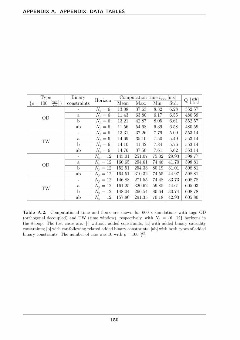
APPENDIX A. APPENDIX: DATA TABLES
Type Binary Horizon Computation time topt [ms] Q[veh
h
](ρ = 100
[vehkm
])constraints Mean Max. Min. Std.
OD
- Np = 6 13.08 37.63 8.32 6.28 552.57a Np = 6 11.43 63.80 6.17 6.55 480.59b Np = 6 13.21 42.87 8.05 6.61 552.57ab Np = 6 11.56 54.68 6.39 6.58 480.59
TW
- Np = 6 13.31 37.26 7.79 5.09 553.14a Np = 6 14.69 35.10 7.50 5.49 553.14b Np = 6 14.10 41.42 7.84 5.76 553.14ab Np = 6 14.76 37.50 7.61 5.62 553.14
OD
- Np = 12 145.01 251.07 75.02 29.93 598.77a Np = 12 160.65 294.61 74.46 41.70 598.81b Np = 12 152.51 254.33 80.19 31.01 598.81ab Np = 12 164.51 310.32 74.55 44.97 598.81
TW
- Np = 12 146.88 271.55 74.48 33.73 608.78a Np = 12 161.25 320.62 59.85 44.61 605.03b Np = 12 148.04 266.54 80.64 30.74 608.78ab Np = 12 157.80 291.35 70.18 42.93 605.80
Table A.2: Computational time and flows are shown for 600 s simulations with tags OD(orthogonal decoupled) and TW (time window), respectively, with Np = 6, 12 horizons inthe 8-loop. The test cases are: [-] without added constraints; [a] with added binary causalityconstraints; [b] with car-following related added binary constraints; [ab] with both types of addedbinary constraints. The number of cars was 10 with ρ = 100 veh
km
150
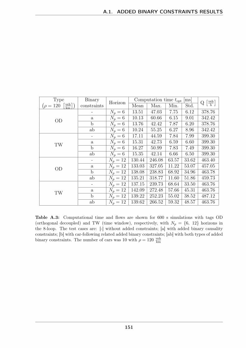
A.1. ADDED BINARY CONSTRAINTS RESULTS
Type Binary Horizon Computation time topt [ms] Q[veh
h
](ρ = 120
[vehkm
])constraints Mean Max. Min. Std.
OD
- Np = 6 13.51 47.03 7.75 6.12 378.76a Np = 6 10.13 60.66 6.15 9.01 342.42b Np = 6 13.76 42.42 7.87 6.20 378.76ab Np = 6 10.24 55.25 6.27 8.96 342.42
TW
- Np = 6 17.11 44.59 7.84 7.99 399.30a Np = 6 15.31 42.73 6.59 6.60 399.30b Np = 6 16.27 50.99 7.83 7.49 399.30ab Np = 6 15.35 42.14 6.66 6.50 399.30
OD
- Np = 12 130.44 246.08 63.57 33.62 463.40a Np = 12 133.03 327.05 11.22 53.07 457.05b Np = 12 138.08 238.83 68.92 34.96 463.78ab Np = 12 135.21 318.77 11.60 51.86 459.73
TW
- Np = 12 137.15 239.73 68.64 33.50 463.76a Np = 12 142.09 272.48 57.66 45.31 463.76b Np = 12 139.22 252.23 55.02 38.52 487.12ab Np = 12 139.62 266.52 59.32 48.57 463.76
Table A.3: Computational time and flows are shown for 600 s simulations with tags OD(orthogonal decoupled) and TW (time window), respectively, with Np = 6, 12 horizons inthe 8-loop. The test cases are: [-] without added constraints; [a] with added binary causalityconstraints; [b] with car-following related added binary constraints; [ab] with both types of addedbinary constraints. The number of cars was 10 with ρ = 120 veh
km
151

152
BAppendix: Road inlet flow generation
For traffic simulation purposes a vehicle arrival model can be used to generate the trafficflow at road inlets.
This appendix aims to enumerate the Poisson distribution, as well as the closely re-lated negative exponential distribution and its relevant measures [10], to then derive thegeneral truncated exponential distribution for vehicle flow at the junction inlets. By us-ing the design parameters of the truncated exponential distribution, random numbers aregenerated via the quantile function sampling.
Definitions and relations that are repeatedly used in the derivations are collected first[10].Definition of expected value, mean, or first moment of a continuous random variable X:
E [X] =
∫ ∞−∞
x f (x) dx,
where the Probability Density Function (PDF) is f of the hypothetical outcome x. In thecase where X is a discrete random variable, the expected value is:
E [X] =∞∑i=1
xi f(xi),
with the probability mass function f of discrete hypothetical outcomes xi.The variance or second central moment (standard deviation squared σ2) of a random
variable X is as follows:
Var [X] = E[(X − E [X])2
]= E
[X2]− E [X]2 . (B.1)
Below, some frequent integrals and their solutions are shown; first:∫eαx dx =
1
αeαx. (B.2)
153
APPENDIX B. APPENDIX: ROAD INLET FLOW GENERATION
The next integral is:∫xeαx dx,
which is solved with integration by parts:∫u (x) v′ (x) dx = u (x) v (x)−
∫v (x) u (x) dx
with substitution of:
u (x) = x; u′ (x) = 1
v′ (x) = eαx; v (x) =
∫v′ (x) dx =
1
αeαx
gives:∫xeαx dx = x
1
αeαx −
∫1
aeαx dx
=
(x
α− 1
α2
)eαx. (B.3)
The following integral is:∫x2eαx dx,
which similarly can be solved using integration by parts, with substitution of:
u (x) = x; u′ (x) = 1
v′ (x) = xeαx; v (x) =
∫v′ (x) dx =
(x
α− 1
α2
)eαx
yields:∫x2eαx dx = x
(x
α− 1
α2
)eαx −
∫ (x
α− 1
α2
)eαxdx
= x
(x
α− 1
α2
)eαx − 1
α
(x
α− 1
α2
)eαx +
1
α3eαx.
In summary:∫x2eαx dx =
(x2
α− 2x
α2+
2
α3
)eαx. (B.4)
Poisson distribution describes the probability of discrete events observed in identicalconsecutive intervals (i.e. the number of vehicles arriving at a fixed point in the road
154
within a defined time period).The probability mass function is defined as:
f (xi) =λxie−λ
xi!,
for the number of hypothetical discrete events xi = 0, 1, 2 . . . (number of vehicles arriving)which occurs with the expected rate value (average number of arrivings) λ > 0 over theinterval.
Expected value (mean) and variance properties of the Poisson distribution with X
discrete random variable:
E [X] =∞∑x=0
x f(x) =∞∑x=0
xλxe−λ
x!=∞∑x=1
xλxe−λ
x!= λe−λ
∞∑x=1
λx−1
(x− 1)!
= λe−λ∞∑x=0
λx
x!= λe−λe = λ.
Using the following expected value identity:
E[X + Y ] = E [X] + E [Y ]
gives:
E[X2]
= E [X (X − 1) +X] = E [X (X − 1)] + E [X] ,
where
E [X (X − 1)] =∞∑x=0
x (x− 1) f(x) =∞∑x=2
x (x− 1)λxe−λ
x!= λ2e−λ
∞∑x=2
λx−2
(x− 2)!
= λ2e−λeλ = λ2.
Thus, by substituting back the above results into (B.1), the variance yields:
Var [X] = E[X2]− E [X]2 = E [X (X − 1)] + E [X]− E [X]2 = λ.
In summary:
E [X] = λ
Var [X] = λ.
One may be more inclined to obtain the distribution of ∆t time gaps between thediscrete events (continuous measure) rather than the number of events over a fixed interval.This formulation of the Poisson process is known as exponential distribution with the
155
APPENDIX B. APPENDIX: ROAD INLET FLOW GENERATION
probability distribution function:
f (y) = λe−λy,
where the rate parameter is λ > 0 and y is defined over [0,∞) interval. Since the PDF ofexponential distribution is continuous, for Y exponentially distributed random variablethe mean and variance over the semi-infinite interval:
E [Y ] =
∫ ∞0
y f(y) dy =
∫ ∞0
y λe−λy dy.
This expression can be solved using the integration-by-parts identity:∫u (x) v′ (x) dx = u (x) v (x)−
∫v (x) u (x) dx
with a substitution of:
u (x) = x; u′ (x) = 1
v′ (x) = eαx; v (x) =
∫v′ (x) dx =
1
αeαx
reaching:∫xeαx dx = x
1
αeαx −
∫1
aeαx dx =
(x
α− 1
α2
)eαx.
Then
E [Y ] =
∫ ∞0
y λe−λy dy = λ
[(−yλ− 1
λ2
)e−λy
]∞0
= λ−1.
In case of the variance:
Var [Y ] =
∫ ∞0
y2f(y)dτ − E [Y ]2 =
∫ ∞0
y2λe−λτdτ − λ−2.
Finally, using the integral (B.4) and the expected value sub-results from above:
Var [Y ] =
∫ ∞0
y2λe−λτdτ − λ−2 =
[(y2 − 2y
λ− 2
λ2
)e−λy
]∞0
− λ−2
= 2λ−2 − λ−2 = λ−2.
In summary:
E [Y ] = λ−1
Var [Y ] = λ−2.
156

Remark: The inlet can now generate vehicle-arrival time gaps according to an expo-nential distribution over the interval of [0,∞). However, with relatively low probability,very high following times could occur, resulting in a rather uneventful simulation. On theother hand, generating vehicle arrival times close to each other would mean that a vehiclecannot yet physically leave the space on the road before the next agent would have toappear in that same spot. This phenomenon remains a disadvantageous characteristic ofthe inlet with a hard demand on vehicles appearing, whereby adding a lower bound onthe following times decreases the number of hard exceptions to be treated.
For more general and flexible settings on the inlet mechanism, a lower- and upper-truncated exponential distribution is formulated with a settable mean. This distributionis later sampled to create Z continuous random variables to express vehicle headways atthe inlet.
f (z) :=
ϕψeϕz, a < Z ≤ b
0, otherwise
where the lower limit is a and the upper limit of truncation is b, moreover, b− a > 0; theparameters defining the general shape of the PDF are ϕ and ψ.
The Cumulative Density Function (CDF) is calculated from the PDF by:
F (z) =
∫ z
−∞f (z) dz.
Moreover, the PDF is chosen to give:
F (a) = 0 (B.5)
F (b) = 1. (B.6)
One more design element is the mean value ω which must lie within the boundariesa < ω < b:
E [Z] =
∫ b
a
z f (z) dz = ω
First, (B.5) and (B.6) conditions are met by:∫ b
a
f (z) dz = 1
∫ b
a
ϕ
ψeϕz dz =
1
ψ[eϕz]ba =
(eϕb − eϕa
)ψ
= 1
157
APPENDIX B. APPENDIX: ROAD INLET FLOW GENERATION
ψ = eϕb − eϕa. (B.7)
Then, the condition for the mean is used:
ω =
∫ b
a
z f (z) dz =
∫ b
a
zϕ
ψeϕz dz =
1
ψ
[(z − 1
ϕ
)eϕz]ba
=1
ψ
(b− 1
ϕ
)eϕb − 1
ψ
(a− 1
ϕ
)eϕa.
Substituting the results from (B.7) gives:
ω = b+(b− a)
eϕ(b−a) − 1− 1
ϕ
which contains ϕ in an implicit manner and can be solved with a generic numerical solver(e.g. fzero in Matlab). This truncation is formulated only for practical use; better variablechoices and more elegant formulae can be obtained.
The derived truncated distribution can describe not only truncated negative expo-nential distributions but also positive exponential distributions, which would apply, forexample, if vehicles were tend to have longer following times more often than short ones.In traffic flows, however, this is not a characteristic trend; in fact, vehicles tend to haveshort following times more often, resulting in negative exponential trends.
B.1 Sampling the truncated exponential distribution
Recall the CDF:
F (z) =
∫ z
a
f (z) dz =
∫ z
a
ϕ
ψeϕzdz =
eϕz − eϕa
ψ.
Thus, the quantile function is:
F−1 (p) =ln (ψp+ eϕa)
ϕ, 0 ≤ p < 1
where the probability is p.After substituting p element wise from a vector of uniformly distributed random num-
bers, with elements on a [0, 1) interval, a sampled, truncated, exponentially distributedrandom number vector can be generated for the vehicle headway times.
158
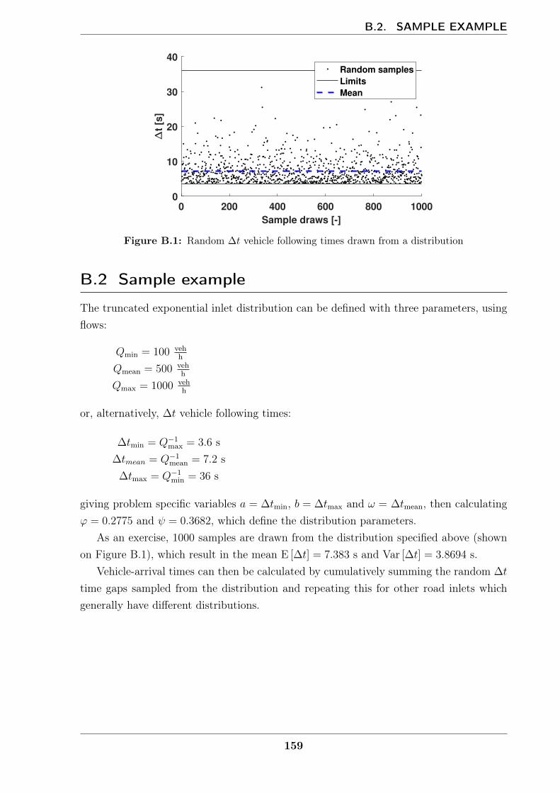
B.2. SAMPLE EXAMPLE
0 200 400 600 800 1000
Sample draws [-]
0
10
20
30
40
t [s
]
Random samples
Limits
Mean
Figure B.1: Random ∆t vehicle following times drawn from a distribution
B.2 Sample example
The truncated exponential inlet distribution can be defined with three parameters, usingflows:
Qmin = 100 vehh
Qmean = 500 vehh
Qmax = 1000 vehh
or, alternatively, ∆t vehicle following times:
∆tmin = Q−1max = 3.6 s∆tmean = Q−1mean = 7.2 s
∆tmax = Q−1min = 36 s
giving problem specific variables a = ∆tmin, b = ∆tmax and ω = ∆tmean, then calculatingϕ = 0.2775 and ψ = 0.3682, which define the distribution parameters.
As an exercise, 1000 samples are drawn from the distribution specified above (shownon Figure B.1), which result in the mean E [∆t] = 7.383 s and Var [∆t] = 3.8694 s.
Vehicle-arrival times can then be calculated by cumulatively summing the random ∆t
time gaps sampled from the distribution and repeating this for other road inlets whichgenerally have different distributions.
159

160
Bibliography
[1] Altche, F.: 2018, Decision-based motion planning for cooperative and autonomous vehicles,Theses, PSL Research University.URL: https://pastel.archives-ouvertes.fr/tel-02073593
[2] Altche, F., Qian, X. and de La Fortelle, A.: 2016, Time-optimal coordination of mobilerobots along specified paths, 2016 IEEE/RSJ International Conference on Intelligent Robotsand Systems (IROS), IEEE.
[3] Altche, F., Qian, X. and de La Fortelle, A.: 2017, An Algorithm for Supervised Driving ofCooperative Semi-Autonomous Vehicles, IEEE Transactions on Intelligent TransportationSystems 18(12), 3527–3539.
[4] Athans, M.: 1969, A unified approach to the vehicle-merging problem, Transportation Re-search 3(1), 123–133.
[5] Bali, C. and Richards, A.: 2017, Robot navigation using convex model predictive controland approximate operating region optimization, 2017 IEEE/RSJ International Conferenceon Intelligent Robots and Systems (IROS), IEEE, pp. 2171–2176.
[6] Bali, C. and Richards, A.: 2018, Merging Vehicles at Junctions using Mixed-Integer ModelPredictive Control, 2018 European Control Conference (ECC), IEEE, pp. 1740–1745.
[7] BBC: Tesla Model 3: Autopilot engaged during fatal crash: 2019,https://www.bbc.co.uk/news/technology-48308852.
[8] Bemporad, A. and Morari, M.: 1999, Control of Systems integrating Logic Dynamics andConstraints, Automatica 35(3), 407–427.
[9] Blanchini, F.: 1999, Set invariance in control, Automatica 35(11), 1747–1767.
[10] Blitzstein, J. K. and Hwang, J.: 2019, Introduction to Probability, Second Edition, Taylor& Francis Ltd.
[11] Borrelli, F., Bemporad, A. and Morari, M.: 2017, Predictive Control for Linear and HybridSystems, Cambridge University Press.
161

BIBLIOGRAPHY
[12] Campbell, M., Egerstedt, M., How, J. P. and Murray, R. M.: 2010, Autonomous driving inurban environments: approaches, lessons and challenges, Philosophical Transactions of theRoyal Society A: Mathematical, Physical and Engineering Sciences 368(1928), 4649–4672.
[13] Carson III, J. M.: 2008, Robust model predictive control with a reactive safety mode, PhDthesis, California Institute of Technology.
[14] Chen, L. and Englund, C.: 2016, Cooperative intersection management: A survey, IEEETransactions on Intelligent Transportation Systems 17(2), 570–586.
[15] Csorvasi, G. and Vajk, I.: 2016, Analysis of an on-line minimum-time velocity optimizationalgorithm, 2016 17th International Carpathian Control Conference (ICCC), IEEE, pp. 122–127.
[16] CVX Research, Inc.: 2012, CVX: Matlab software for disciplined convex programming,version 2.0, http://cvxr.com/cvx.
[17] Dahl, J., de Campos, G. R., Olsson, C. and Fredriksson, J.: 2019, Collision avoidance: Aliterature review on threat-assessment techniques, IEEE Transactions on Intelligent Vehicles4(1), 101–113.
[18] de Campos, G. R., Falcone, P., Hult, R., Wymeersch, H. and Sjoberg, J.: 2017, Trafficcoordination at road intersections: Autonomous decision-making algorithms using model-based heuristics, IEEE Intelligent Transportation Systems Magazine 9(1), 8–21.
[19] de Campos, G. R., Falcone, P. and Sjoberg, J.: 2013, Autonomous cooperative driving:A velocity-based negotiation approach for intersection crossing, 16th International IEEEConference on Intelligent Transportation Systems (ITSC 2013), IEEE.
[20] de La Fortelle, A.: 2010, Analysis of reservation algorithms for cooperative planning atintersections, 13th International IEEE Conference on Intelligent Transportation Systems,IEEE.
[21] Debada, E., Makarem, L. and Gillet, D.: 2017, A virtual vehicle based coordination frame-work for autonomous vehicles in heterogeneous scenarios, 2017 IEEE International Confer-ence on Vehicular Electronics and Safety (ICVES), IEEE.
[22] Dresner, K. and Stone, P.: 2004, Multiagent traffic management: A reservation-based in-tersection control mechanism, Proceedings of the Third International Joint Conference onAutonomous Agents and Multiagent Systems - Volume 2, AAMAS ’04, IEEE ComputerSociety, Washington, DC, USA, pp. 530–537.
[23] Dunbar, W. B. and Murray, R. M.: 2006, Distributed receding horizon control for multi-vehicle formation stabilization, Automatica 42(4), 549–558.
[24] Eele, A. and Richards, A. G.: 2007, Path-planning with avoidance using nonlinear branch-and-bound optimisation, AIAA Guidance, Navigation and Control Conference.
162
BIBLIOGRAPHY
[25] ERSO: 2018, Traffic safety basic facts (latest data: 2016), online. European Road SafetyObservatory (ERSO).
[26] Fankhauser, B., Makarem, L. and Gillet, D.: 2011, Collision-free intersection crossing ofmobile robots using decentralized navigation functions on predefined paths, 2011 IEEE 5thInternational Conference on Cybernetics and Intelligent Systems (CIS), IEEE.
[27] Flores, C., Milanes, V. and Nashashibi, F.: 2017, A time gap-based spacing policy for full-range car-following, 2017 IEEE 20th International Conference on Intelligent TransportationSystems (ITSC), IEEE.
[28] Grant, M. and Boyd, S.: 2008, Graph implementations for nonsmooth convex programs,in V. Blondel, S. Boyd and H. Kimura (eds), Recent Advances in Learning and Control,Lecture Notes in Control and Information Sciences, Springer-Verlag Limited, pp. 95–110.
[29] Greatwood, C. and Richards, A. G.: 2019, Reinforcement learning and model predictive con-trol for robust embedded quadrotor guidance and control, Autonomous Robots 43(7), 1681–1693.
[30] Gregoire, J.: 2014, Priority-based coordination of mobile robots, PhD thesis, Mines Par-isTech.
[31] Gregoire, J., Bonnabel, S. and de La Fortelle, A.: 2013, Robust multirobot coordinationusing priority encoded homotopic constraints, p. 21.
[32] Gurobi Optimization, LLC: 2019, Gurobi Optimizer Reference Manual.URL: http://www.gurobi.com
[33] Haklay, M. and Weber, P.: 2008, OpenStreetMap: User-generated street maps, IEEE Per-vasive Computing 7(4), 12–18.
[34] Hult, R., Zanon, M., Gras, S. and Falcone, P.: 2018, An MIQP-based heuristic for OptimalCoordination of Vehicles at Intersections, 2018 IEEE Conference on Decision and Control(CDC), IEEE, pp. 2783–2790.
[35] Hult, R., Zanon, M., Gros, S. and Falcone, P.: 2016, Primal decomposition of the optimalcoordination of vehicles at traffic intersections, 2016 IEEE 55th Conference on Decision andControl (CDC), IEEE.
[36] Hult, R., Zanon, M., Gros, S., Wymeersch, H. and Falcone, P.: 2019, Optimization-basedcoordination of connected, automated vehicles at intersections. Vehicle System Dynamics.
[37] INRIX 2018 Global Traffic Scorecard: 2019, online.URL: http://inrix.com/press-releases/scorecard-2018-uk/
[38] Jung, M.: 2014, Relaxations and approximations for mixed-integer optimal control.
163
BIBLIOGRAPHY
[39] Kamal, M. A. S., ichi Imura, J., Hayakawa, T., Ohata, A. and Aihara, K.: 2015, A vehicle-intersection coordination scheme for smooth flows of traffic without using traffic lights, IEEETransactions on Intelligent Transportation Systems 16(3), 1136–1147.
[40] Kant, K. and Zucker, S. W.: 1986, Toward efficient trajectory planning: The path-velocitydecomposition, The International Journal of Robotics Research 5(3), 72–89.
[41] Kerrigan, E. C. and Maciejowski, J. M.: 2000, Soft Constraints And Exact Penalty FunctionsIn Model Predictive Control, Control 2000 Conference .
[42] Kerrigan, E. and Maciejowski, J.: 2001, Robust feasibility in model predictive control:necessary and sufficient conditions, Proceedings of the 40th IEEE Conference on Decisionand Control (Cat. No.01CH37228), Vol. 1, IEEE, pp. 728–733.
[43] Kim, K.-D. and Kumar, P. R.: 2014, An MPC-based approach to provable system-widesafety and liveness of autonomous ground traffic, IEEE Transactions on Automatic Control59(12), 3341–3356.
[44] Kowshik, H., Caveney, D. and Kumar, P. R.: 2011, Provable systemwide safety in intelligentintersections, IEEE Transactions on Vehicular Technology 60(3), 804–818.
[45] LaValle, S.: 2006, Planning Algorithms, Cambridge University Press.
[46] Levinson, J., Askeland, J., Becker, J., Dolson, J., Held, D., Kammel, S., Kolter, J. Z.,Langer, D., Pink, O., Pratt, V., Sokolsky, M., Stanek, G., Stavens, D., Teichman, A., Wer-ling, M. and Thrun, S.: 2011, Towards fully autonomous driving: Systems and algorithms,2011 IEEE Intelligent Vehicles Symposium (IV), IEEE.
[47] Luo, L., Chen, J. and Zhang, F.: 2016, Integrated adaptive cruise control design consideringthe optimization of switching between throttle and brake, 2016 IEEE Intelligent VehiclesSymposium (IV), IEEE.
[48] Maciejowski, J.: 2000, Predictive Control with Constraints, Prentice Hall.
[49] Maestre, J. M. and Negenborn, R. R. (eds): 2014, Distributed Model Predictive ControlMade Easy, Springer Netherlands.
[50] Maia, M. H. and Galvão, R. K. H.: 2009, On the use of mixed-integer linear programming forpredictive control with avoidance constraints, International Journal of Robust and NonlinearControl 19(7), 822–828.
[51] Makarem, L. and Gillet, D.: 2012, Fluent coordination of autonomous vehicles at inter-sections, 2012 IEEE International Conference on Systems, Man, and Cybernetics (SMC),IEEE.
[52] Makarem, L. and Gillet, D.: 2013, Model predictive coordination of autonomous vehiclescrossing intersections, 16th International IEEE Conference on Intelligent TransportationSystems (ITSC 2013), IEEE.
164

BIBLIOGRAPHY
[53] Mayne, D. Q., Rawlings, J. B., Rao, C. V. and Scokaert, P. O. M.: 2000, Constrained ModelPredictive Control: Stability and Optimality, Automatica 36, 789–814.
[54] Paden, B., Cap, M., Yong, S. Z., Yershov, D. and Frazzoli, E.: 2016, A survey of mo-tion planning and control techniques for self-driving urban vehicles, IEEE Transactions onIntelligent Vehicles 1(1), 33–55.
[55] Pande, A.: 2015, Traffic engineering handbook, John Wiley & Sons Inc, Hoboken, NewJersey.
[56] Prodan, I., Stoican, F., Olaru, S. and Niculescu, S.-I.: 2016, Mixed-Integer Representationsin Control Design, Springer International Publishing.
[57] Qian, X.: 2016, Model predictive control for autonomous and cooperative driving, Theses,PSL Research University.URL: https://pastel.archives-ouvertes.fr/tel-01635261
[58] Qian, X., Gregoire, J., de La Fortelle, A. and Moutarde, F.: 2015, Decentralized model pre-dictive control for smooth coordination of automated vehicles at intersection, 2015 EuropeanControl Conference (ECC), IEEE, pp. 3452–3458.
[59] Rawlings, J. B., Mayne, D. Q. and Diehl, M. M.: 2017, Model Predictive Control: Theory,Computation, and Design, 2nd Edition, Nob Hill Publishing, LLC.
[60] Richards, A. G.: 2002, Trajectory control using mixed integer linear programming, Master’sthesis, MIT.
[61] Richards, A. G. and How, J. P.: 2005, Mixed-integer Programming for Control, Proceedingsof the American Control Conference, IEEE, Portland, Oregon, pp. 2676–2683.
[62] Richards, A. and How, J. P.: 2007, Robust distributed model predictive control, Interna-tional Journal of Control 80(9), 1517–1531.
[63] Richards, A. and Turnbull, O.: 2013, Inter-sample avoidance in trajectory optimizers usingmixed-integer linear programming, International Journal of Robust and Nonlinear Control25(4), 521–526.
[64] Rios-Torres, J. and Malikopoulos, A. A.: 2017a, Automated and cooperative vehicle mergingat highway on-ramps, IEEE Transactions on Intelligent Transportation Systems 18(4), 780–789.
[65] Rios-Torres, J. and Malikopoulos, A. A.: 2017b, A survey on the coordination of connectedand automated vehicles at intersections and merging at highway on-ramps, IEEE Transac-tions on Intelligent Transportation Systems 18(5), 1066–1077.
[66] Rizaldi, A. and Althoff, M.: 2015, Formalising traffic rules for accountability of autonomousvehicles, 2015 IEEE 18th International Conference on Intelligent Transportation Systems,IEEE.
165
BIBLIOGRAPHY
[67] Rosolia, U., Bruyne, S. D. and Alleyne, A. G.: 2017, Autonomous vehicle control: A non-convex approach for obstacle avoidance, IEEE Transactions on Control Systems Technology25(2), 469–484.
[68] Sathya, A., Sopasakis, P., Parys, R. V., Themelis, A., Pipeleers, G. and Patrinos, P.: 2018,Embedded nonlinear model predictive control for obstacle avoidance using PANOC, 2018European Control Conference (ECC), IEEE.
[69] Scattolini, R.: 2009, Architectures for distributed and hierarchical Model Predictive Control– A review, Journal of Process Control 19(5), 723–731.
[70] Schouwenaars, T., Moor, B. D., Feron, E. and How, J.: 2001, Mixed integer programmingfor multi-vehicle path planning, 2001 European Control Conference (ECC), IEEE.
[71] Shi, J., Zheng, Y., Jiang, Y., Zanon, M., Hult, R. and Houskal, B.: 2018, Distributedcontrol algorithm for vehicle coordination at traffic intersections, 2018 European ControlConference (ECC), IEEE, pp. 1166–1171.
[72] Shin, Y. and Bien, Z.: 1989, Collision–Free Trajectory Planning for Two Robot Arms,Robotica 7(03), 205.
[73] Singh, S.: 2018, Critical reasons for crashes investigated in the national motor vehiclecrash causation survey, Technical Report DOT HS 812 506, National Highway Traffic SafetyAdministration, Washington, DC.
[74] Thrun, S.: 2010, Toward robotic cars, Communications of the ACM 53(4), 99.
[75] Treiber, M. and Kesting, A.: 2013, Traffic Flow Dynamics, Springer Berlin Heidelberg.
[76] Trodden, P. A. and Richards, A. G.: 2013, Cooperative tube-based distributed MPC forlinear uncertain systems coupled via constraints, Intelligent Systems, Control and Automa-tion: Science and Engineering, (Distributed Model Predictive Control Made Easy), SpringerNetherlands, pp. 57–72.
[77] UK Department for Transport: 2015, The Highway Code, available athttps://www.gov.uk/guidance/the-highway-code.
[78] Urmson, C., Anhalt, J., Bagnell, D., Baker, C., Bittner, R., Clark, M. N., Dolan, J.,Duggins, D., Galatali, T., Geyer, C., Gittleman, M., Harbaugh, S., Hebert, M., Howard,T. M., Kolski, S., Kelly, A., Likhachev, M., McNaughton, M., Miller, N., Peterson, K.,Pilnick, B., Rajkumar, R., Rybski, P., Salesky, B., Seo, Y.-W., Singh, S., Snider, J., Stentz,A., Whittaker, W. “., Wolkowicki, Z., Ziglar, J., Bae, H., Brown, T., Demitrish, D., Litkouhi,B., Nickolaou, J., Sadekar, V., Zhang, W., Struble, J., Taylor, M., Darms, M. and Ferguson,D.: 2008, Autonomous driving in urban environments: Boss and the Urban Challenge,Journal of Field Robotics 25(8), 425–466.
166
BIBLIOGRAPHY
[79] Velenis, E. and Tsiotras, P.: 2008, Minimum-time travel for a vehicle with accelerationlimits: Theoretical analysis and receding-horizon implementation, Journal of OptimizationTheory and Applications 138(2), 275–296.
[80] Wakabayashi, D.: 2018, Self-driving uber car kills pedestrian in arizona, where robots roam,The New York Times, online.URL: https://www.nytimes.com/2018/03/19/technology/uber-driverless-fatality.html
[81] Wang, Y. and Boyd, S.: 2010, Fast model predictive control using online optimization,IEEE Transactions on Control Systems Technology 18(2), 267–278.
[82] Williams, H. P. and Brailsford, S. C.: 1996, Advances in Linear and Integer Programming,Clarendon Press, Oxford, UK, chapter Computational Logic and Integer Programming,pp. 249–281.
[83] Xu, S. and Peng, H.: 2018, Design and comparison of fuel-saving speed planning algorithmsfor automated vehicles, IEEE Access 6, 9070–9080.
[84] Yi, B., Gottschling, S., Ferdinand, J., Simm, N., Bonarens, F. and Stiller, C.: 2016, Realtime integrated vehicle dynamics control and trajectory planning with MPC for criticalmaneuvers, 2016 IEEE Intelligent Vehicles Symposium (IV), IEEE.
[85] Zhang, Y. J., Malikopoulos, A. A. and Cassandras, C. G.: 2016, Optimal control and co-ordination of connected and automated vehicles at urban traffic intersections, 2016 Amer-ican Control Conference (ACC), IEEE.
167

168
Related Documents