Driver steering assistance for lane departure avoidance

Driver steering assistance for lane departure

avoidance

N. Minoiu Enache a,∗,1, M. Netto a, S. Mammar b, B. Lusetti a

aLCPC/INRETS - LIVIC Laboratoire sur les Interactions

Vehicules-Infrastructure-Conducteurs, 14 route de la miniere, 78000 Versailles, France

bIBISC/CNRS-FRE 3190, Universite d’Evry Val d’Essonne, 40 Rue du Pelvoux, CE 1455,

91025, Evry, Cedex, France

Abstract

In this paper, a steering assistance system is designed and experimentally tested on a proto-

type passenger vehicle. Its main goal is to avoid lane departures when the driver has a lapse

of attention. Based on a concept linking Lyapunov theory with Linear Matrix Inequali-

ties (LMI) optimization, the following important features are ensured during the assistance

intervention: the vehicle remains within the lane borders while converging towards the cen-

terline, and the torque control input and the vehicle dynamics are limited to safe values to

ensure the passengers’ comfort. Because the steering assistance takes action only if nec-

essary, two activation strategies have been proposed. Both activation strategies were tested

on the prototype vehicle and were assessed as appropriate. However, the second strategy

showed better reactivity in case of rapid drifting out of the lane.

Key words: active safety, lane departure avoidance, lateral vehicle control, Lyapunov

function, LMI, switched system

Preprint submitted to Control Engineering Practice 21 October 2008

1 Introduction

The failure of a driver to remain in the correct lane due to inattention, illness, or

sleepiness is one of the most important causes of accidents. NHTSA (2006) esti-

mated that running off the road caused about 28% of the fatal motor vehicle crashes

in the US in 2005. Moreover, drowsy, sleeping, or fatigued drivers and inattentive

drivers caused about 2.6% and 5.8% of the fatal crashes, respectively.

In order to prevent this type of accident, vehicles have increasingly been equipped

with electronic control systems that provide active safety (Isermann (2008)). New

steering assistance systems have been developed both to decrease the driver’s work-

load and to prevent lane departures (Shimakage et al. (2002)), (Rossetter et al.

(2004)), (LeBlanc et al. (1996)) and (Nagai et al. (2002)). Eidehall et al. (2007)

proposed an integrated road geometry estimation method using vehicle tracking to

improve the activation accuracy of an emergency lane assist system.

The work presented in this paper aims at developing a steering assistance system

that helps the driver guide the vehicle to the center of the lane during diminished

driving capability due to inattention, fatigue, or illness. For vehicles equipped with

a conventional steering column, an important issue in implementing a steering as-

sistance system arises: How to introduce automation to help the driver simultane-

ously with his own actions on the steering wheel? Any intrusion by an automatic

steering system might be immediately felt by the driver on the steering wheel. Re-

∗ Corresponding author.Email addresses: [email protected] (N. Minoiu Enache),

[email protected] (M. Netto), [email protected] (S.

Mammar), [email protected] (B. Lusetti).1 Tel. +33-(0)1-40432919; fax +33-(0)1-40432930.

2

ciprocally, any torque imposed on the steering wheel by the driver could be consid-

ered by the automatic control system as a disturbance input.

To overcome this difficulty, a switching strategy coupled with a designed lateral

control law is proposed in this work. The switching strategy assigns the steering

control either to the driver or to the steering assistance system. More specifically,

the steering assistance system has been developed to take over the driver’s action

when it is determined that he has lost attention and to return control of the vehicle

upon the driver’s request when the vehicle is out of danger.

The main contributions of this paper are:

(1) A theoretical framework for handling the interactions between the driver and

the steering assistance system that ensures bounded dynamics of the switched

system.

(2) Guaranteed bounds for the displacement of the front wheels with respect to

the center of the lane, as well as a control torque input that is limited by the

design method during the assistance intervention.

(3) Validation of the theoretical results by experimental tests using a prototype

vehicle.

The contents of this paper are organized as follows. Section 2 presents the vehicle

model, including the electrically powered steering column. The specifications of

the steering assistance system are given in Section 3.1, while Sections 3.2 and 3.3

address the definition of a “normal driving” situation and the design of the switch-

ing strategy. Sections 4 and 5 describe the design of the steering control law, and

subsequently the evolution of the trajectories of the switched system. Section 6 con-

tains the results of the practical implementation of the steering assistance system

under the first switching strategy. Following these results, new activation rules for

3

a second switching strategy are developed and practically implemented in Section

7. Conclusions are presented in Section 8.

2 Vehicle model with electrically powered steering

Since this study is focused on the lateral control of a vehicle, a classical fourth

order linear model (“bicycle model”, Fig. 1) was used (Ackermann et al. (1995)).

The effect of road curvature was neglected and the road was assumed to be straight,

which is realistic for the highway driving environment addressed in this work. The

steering torque necessary for the assistance is provided by a DC motor mounted

on the steering column, for which a second order model was adopted. The vehicle

model, including the electrical steering assistance model, is given by:

x = A ·x+B · (Ta +Td), (1)

A =

a11 a12 0 0 b1 0

a21 a22 0 0 b2 0

0 1 0 0 0 0

v lS v 0 0 0

0 0 0 0 0 1

TSβISRS

TSrISRS

0 0 −2Kpc f ηt

ISR2S−BS

IS

, (2)

4

B =

(0, 0, 0, 0, 0, 1

RSIS

)T

, (3)

where

a11 =−2(cr+c f )mv , a12 =−1+ 2(lrcr−l f c f )

mv2 ,

a21 = 2(lrcr−l f c f )J , a22 =−2(l2

r cr+l2f c f )

Jv ,

cr = cr0µ, c f = c f 0µ,

b1 = 2c fmv , b2 = 2c f l f

J ,

TSβ = 2Kpc f ηtRS

, TSr = 2Kpc f l f ηtRSv .

(4)

The definitions and the numerical values of the above parameters are given in Table

2 at the end of the paper. The state vector is x , (β ,r,ψL,yL,δ f , δ f )T , where β

denotes the side slip angle, r is the yaw rate, ψL is the relative yaw angle, yL is the

lateral offset with respect to the lane centerline at a look-ahead distance lS, δ f is

the steering angle, and δ f is its derivative. The inputs for the system given in Eq.

(1) are the driver’s torque Td and the assistance torque Ta. The whole state vector is

considered to be available for measurement.

Remark 1 It can easily be shown that the system given in Eq. (1) is controllable

except for a longitudinal speed v equal to zero. The matrix A has two poles at the

origin, indicating instability of the linear system.

5

Fig. 1. Vehicle “bicycle” model.

3 Steering assistance requirements and problem formulation

3.1 Steering assistance requirements

The proposed steering assistance system aims at avoiding unintended lane depar-

tures during “normal driving”. “Normal driving” is defined as a driving situation

during which the driver is following the center of the lane without performing any

special maneuver (e.g., overtaking, cornering, change of direction). The steering

assistance system should accomplish its task by means of two intelligent modules:

(1) A switching strategy module that activates and deactivates the steering assis-

tance system depending on the driver’s attention and on the danger of lane

departure.

(2) A second module that contains a steering control law should drive the vehicle

during the driver’s inattention. The steering control law should satisfy the fol-

lowing requirements: (a) the closed loop system vehicle-steering control law

6

Fig. 2. Vehicle in the lane.

has to be asymptotically stable to zero steady state, (b) the vehicle shall not

cross the lane borders during the assistance intervention period, (c) moreover,

the overshoot of the front wheels with respect to a fixed predefined center lane

strip has to be as small as possible, and (d) the vehicle state variables and the

steering assistance torque have to be bounded to guarantee safety and comfort.

3.2 Mathematical definition of the “normal driving” zone

First of all, the qualitative description of the “normal driving” situation has to be

transposed into a formal mathematical description. Such a driving situation can

been characterized by the positions of the vehicle’s front wheels, which are gener-

ally confined to a strip along the center of the lane during a normal lane keeping

maneuver. This center strip is assumed to have a width of 2d, where the total lane

width is L and 2d < L, as shown in Fig. 2. On the other hand, during “normal

driving”, the vehicle state variables are assumed to have a limited range, bounded

within a region in the state space. This region was defined by the maximum absolute

values: |β | ≤ β N , |r| ≤ rN , |ψL| ≤ ψNL , |yL| ≤ yN

L , |δ f | ≤ δ Nf and |δ f | ≤ δ N

f .

The coordinates of the two front wheels yl and yr are calculated with respect to

7

the center of the lane from the geometrical model in Fig. 2. The relative position

of the vehicle with respect to the lane, represented in Fig. 2, is characterized by a

relative yaw angle ψL, a lateral offset from the centerline yCGL at the vehicle center

of gravity, and a lateral offset yL measured at a look-ahead distance lS 2 . Assuming

a small relative yaw angle ψL, the following equalities can be written:

yl = yCGL + l f ψL + a

2 ,

yr = yCGL + l f ψL− a

2 ,

(5)

where l f is the distance from the vehicle center of gravity to the front axle and a

is the vehicle width 3 . Generally, the vehicle road sensing system used for lateral

control is limited to a camera mounted with a frontal view and image processing

algorithms to measure the lateral offset and the relative yaw angle. For this reason,

for a straight road and for a small angle ψL, the following equality containing yL

was deduced from Eq. (5) by using the approximation yCGL∼= yL − lS ·ψL, as is

shown in Fig. 2:

yl = yL +(l f − lS)ψL +a2, yr = yL +(l f − lS)ψL− a

2. (6)

From Eq. (6), the condition that the coordinates of the front wheels yl and yr are

located simultaneously inside the fixed center lane strip ±d can been written as:

−2d−a2

≤ yL +(l f − lS)ψL ≤ 2d−a2

. (7)

2 The lateral offsets yCGL and yL are considered positive on the left side of the lane. The

relative yaw angle ψL is considered positive for trigonometric rotations with the origin in

the centerline.3 Values for the parameters l f and a are given in Table 2 at the end of the paper.

8

Hence, the state x that fulfills the above inequalities (7) belongs to the set

L(F) , {x ∈ R6 : |Fx| ≤ 1}, (8)

where F ∈ R1×6, F = (0, 0,2(l f−lS)

2d−a , 22d−a , 0, 0). This set contains the state space

region between two parallel hyperplanes, which are characterized by the vector F

and |Fx|= 1, as shown in Fig. 3.

Remark 2 As detailed later in Section 3.3, a situation is considered to be danger-

ous when at least one of the two front wheels crosses one of the edges of the center

lane strip ±d, which means |Fx|= 1.

A second characteristic defining “normal driving” is that the vehicle state x remains

in a bounded space region. Supposing that |xi| ≤ xNi for i = 1, . . . ,6, where xi de-

notes the i-th component of the state vector x, then for “normal driving” the state

vector x belongs to the set

L(FN) , {x ∈ R6 : |fNi x| ≤ 1, i = 1, . . . ,6}, (9)

where FN ∈ R6×6, fNi represent the rows of FN , f N

i,i = (xNi )−1 and f N

i, j = 0 for i 6= j,

i, j = 1, . . . ,6. L(FN) represents a hypercube in the state space characterized by the

diagonal matrix FN .

Hence, the formal description of “normal driving” defined by the two above sets is

x ∈ L(F) (see Fig. 3), where

L(F) , L(F)∩L(FN) = {x ∈ R6 : |fix| ≤ 1, fi = fNi , i = 1, . . . ,6 , f7 = F}. (10)

L(F) represents a finite polyhedron in the state-space (a polytope) characterized by

the matrix F ∈ R7×6, F = ((FN)T , FT )T .

9

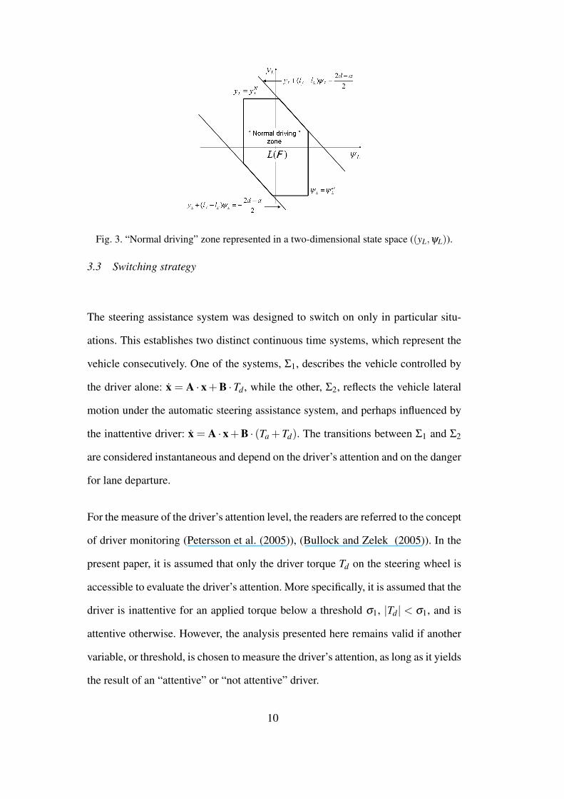
Fig. 3. “Normal driving” zone represented in a two-dimensional state space ((yL,ψL)).

3.3 Switching strategy

The steering assistance system was designed to switch on only in particular situ-

ations. This establishes two distinct continuous time systems, which represent the

vehicle consecutively. One of the systems, Σ1, describes the vehicle controlled by

the driver alone: x = A · x + B ·Td , while the other, Σ2, reflects the vehicle lateral

motion under the automatic steering assistance system, and perhaps influenced by

the inattentive driver: x = A · x + B · (Ta + Td). The transitions between Σ1 and Σ2

are considered instantaneous and depend on the driver’s attention and on the danger

for lane departure.

For the measure of the driver’s attention level, the readers are referred to the concept

of driver monitoring (Petersson et al. (2005)), (Bullock and Zelek (2005)). In the

present paper, it is assumed that only the driver torque Td on the steering wheel is

accessible to evaluate the driver’s attention. More specifically, it is assumed that the

driver is inattentive for an applied torque below a threshold σ1, |Td| < σ1, and is

attentive otherwise. However, the analysis presented here remains valid if another

variable, or threshold, is chosen to measure the driver’s attention, as long as it yields

the result of an “attentive” or “not attentive” driver.

10

The transition from Σ1 to Σ2 switches on the assistance system when a driver’s lack

of attention during “normal driving” may lead to an unintended lane departure 4 :

T 12r : (|Td|< σ1)∧ (x ∈ (L(F)))∧ (|Fx|= 1). (11)

The steering control system has to be switched off (transition from Σ2 to Σ1) when-

ever the driver recovers attention but, for safety reasons, should occur only if the

vehicle is in the “normal driving” zone. However, to handle the case of an emer-

gency situation, the assistance should be removed whenever the driver considers it

necessary and applies a strong torque |Td| ≥ σ2 to the steering wheel. The associ-

ated logical condition is:

T 21r : [(σ1 ≤ |Td|< σ2)∧ (x ∈ (L(F))]∨ (|Td| ≥ σ2). (12)

4 Control law design

This section proposes a control law for the steering torque provided by the DC

motor mounted on the steering column. The main requirements for this control law

are closed loop asymptotic stability, minimal overshoot with respect to the fixed

center lane strip of width 2d, and passengers’ comfort. For the simplicity of the

computation and the implementation, a linear state feedback control is chosen with

a compensation for the driver’s torque: Ta = Kx−Td . Thus, the closed loop system

x = (A + BK)x is obtained from Eq. (1). The following paragraphs express the

control requirements as LMI inequalities that allow the computation of the vector

K.

4 ∧ denotes the logical “and” and ∨ denotes the logical “or”.

11

4.1 Asymptotic stability of the closed loop system

Concerning the system stability, the existence of a Lyapunov function V (x) = xT Px

with P a symmetric, positive definite matrix satisfying (A+BK)T P+P(A+BK)≺0 guarantees the asymptotic stability of the system Σ2. With the bijective trans-

formation Q = P−1 and Y = KQ, the above nonlinear matrix inequality becomes

linear (Boyd et al. (1994)) 5 :

QAT +AQ+BY+YT BT ≺ 0. (13)

4.2 Minimum overshoot with respect to the fixed center lane strip

The ideal behavior of the minimal overshoot problem would be zero overshoot.

That would be possible if the system Σ2 accepted L(F) as a polyhedral invariant

set, since in this case each trajectory that starts in the set L(F) would remain inside

it (for details on the invariant set theory, see (Blanchini (1999))). As this control

objective is difficult to attain for physical and control design reasons, an outer in-

variant approximation of the polyhedron L(F) is used. This approximation is given

by an ellipsoidal set (Minoiu et al. (2006)).

Therefore, an ellipsoid ε = {x : xT Px ≤ 1} is first sought such that it is included

in L(F) and is located as close as possible to the control activation zone (|Fx| =1)∩L(FN) (see Fig. 4). These constraints can be written as LMI expressions (Hu

and Lin (2000)):

5 “≺ 0”, “¹ 0”, denote negative definite, rsp. semi-definite, matrices, “ 0”, “º 0”, denote

positive definite, rsp. semi-definite, matrices.

12

(1) Inclusion of the ellipsoid ε in L(F).

1 fiQ

(fiQ)T Q

º 0, i = 1, . . . ,7, (14)

where fi are the row vectors of the matrix F in Eq. (10).

(2) Approaching the activation zone (|Fx|= 1)∩L(FN).

minimize −α

subject to α ¹ FT QF,

FT QF≺ 1.

(15)

Once found, the ellipsoid ε is expanded until it includes the above mentioned con-

trol activation zone, that is ((|Fx| = 1)∩L(FN)) ⊂ εext = {x : xT Px ≤ Vext} (Fig.

4). This computation is achieved by maximizing the nonlinear function V (x) under

linear constraints:

Vext = max(V (x)) = max(xT Px)

subject to Fx = 1

x ∈ L(FN).

(16)

The LMI optimization problem given in Eq. (15) provides a minimum expansion

of the interior ellipsoid ε to εext .

The quadratic Lyapunov function V (x) = xT Px guarantees that the trajectories of

the system Σ2 will not leave the εext state space region after the assistance system is

activated. Consequently, all system trajectories that start in (|Fx|= 1)∩L(FN) will

not leave the ellipsoidal invariant set εext .

13

Fig. 4. The polyhedron L(F) and the ellipsoids ε and εext , represented in a two-dimensional

state space (yL, ψL).

Furthermore, the hyperplanes tangent to εext and parallel to |Fx|= 1 are equivalent

to the center lane strip of width 2dext , where the two front wheels are guaranteed to

remain during activation of the assistance system (Figs. 2, 4):

dext =2d−a

2

√Vext FQFT +

a2. (17)

4.3 Passengers’ comfort

For comfort reasons, and also for technical reasons, the maximum assistance torque

is bounded at a pre-defined value for vehicle states x ∈ ε , denoted here by TM.

This is achieved by imposing the ellipsoidal invariant set ε to be contained in the

polyhedron L(K) = {x ∈ R6 : |Kx| ≤ TM}, which is equivalent to the following

LMI condition:

1 1TM

Y

1TM

YT Q

º 0. (18)

Furthermore, by expanding the ellipsoid ε to εext , the guaranteed maximum torque

for x ∈ εext is greater than TM. Therefore, the torque limit TM was chosen to be

smaller than the maximum torque supported by the DC motor. In addition, an upper

14

bound of the motor torque used to bring the vehicle to the correct trajectory from a

vehicle state x in εext is given by TMext = maxx∈εext

(Kx) =√

Vext√

KP−1KT .

Putting together the conditions from the above paragraphs 4.1, 4.2, and 4.3, the

feedback control vector K based on the Lyapunov function V (x) = xT Px can be

obtained as a result of the following LMI linear cost optimization problem.

minimize −α

subject to Eq.(13) (system stability),

Eq.(14) (inclusion in the “normal driving” set),

Eq.(15) (approaching the activation zones),

Eq.(18) (bounding the steering torque).

(19)

This LMI optimization problem has Q and Y as matrix variables. P = Q−1 and

K = Q−1Y are obtained afterwards.

The range of the state variables during the assistance intervention can also be con-

sidered to reflect the passengers’ comfort. This range can be computed only a pos-

teriori, after the controller design is completed. Therefore, multiple iterations may

potentially be required to achieve acceptable values. Upper bounds for these vari-

ables are given by projecting the ellipsoid εext on the six state coordinates. These

projections are defined by xMi , where |xi| ≤ xM

i , xMi =

√Qi,i for i = 1, . . . ,6 and Qi,i

is an element of the diagonal of matrix Q.

15

4.4 Robustness against vehicle speed and adhesion variations

The system description given in Eq. (1) depends nonlinearly on the vehicle speed v.

The control law developed in Section 4 provides the required performance only for

a fixed predefined longitudinal velocity v. In this part of the paper, a valid extension

of the control law to a speed interval is proposed.

By choosing ξv ∈ [−1;1], a parameter that describes the variation of v between a

lower limit vmin and an upper limit vmax, the following can be written (Raharijoana

(2004)):

1v

=1v0

+1v1

ξv, v∼= v0(1− v0

v1ξv),

1v2∼= 1

v20(1+2

v0

v1ξv).

(20)

Setting ξv =−1 v = vmin and ξv = 1 v = vmax, v0 and v1 can be written as following:

v0 =2vminvmax

vmax + vmin, v1 =−2(vminvmax)

vmax− vmin. (21)

With these expressions for v, 1/v, and 1/v2, the matrix A of the system given in

Eq. (1) can be written as A = A∗+ A∗∗ξv. Hence, the matrix A(v) evolves into a

matrix polytope for v ∈ [vmin,vmax].

The LMI optimization problem given in Eq. (19) of Section 4 can be modified for a

varying vehicle speed v∈ [vmin,vmax]. Indeed, only the matrix A of the LMI problem

is speed dependent. Due to the linear convex property of the matrix polytope, ineq.

(13) holds for any v ∈ [vmin,vmax] if the following holds:

Q(A∗±A∗∗)T +(A∗±A∗∗)Q+BY+YT BT ≺ 0. (22)

The above considerations mean that if the matrix variables Q and Y are obtained

such that they minimize the LMI problem from Eq. (19), for both A = A∗−A∗∗ and

16

for A = A∗+ A∗∗, then the control vector K stabilizes the system given in Eq. (1)

for any varying speed v ∈ [vmin,vmax], while satisfying the required performance.

As condition (22) is conservative, it may lead to poor performance over the speed

range. Thus, taking into account many speed intervals [vimin,v

imax], [v

i+1min ,v

i+1max], vi+1

min <

vimax, and the corresponding feedback vectors Ki, Ki+1, gain scheduling can be car-

ried out (Stilwell and Rugh (1997)).

The same reasoning can be used for the adhesion µ as for the vehicle speed.

Furthermore, the matrix A already depends linearly on µ . Considering that µ ∈[µmin,1], the vertices of the new matrix polytope are obtained for {µmin,1}. If vari-

ations of both v and µ are considered, the matrix A becomes multi-affine, and thus

a Linear Fractional Representation (LFR) can be adopted (Scherer et al. (1997)).

5 Discussion of the trajectories of the switched system driver-steering assis-

tance

The trajectories of the switched system are briefly analyzed in this Section. This

explains the choice of the switching strategy in Section 3.3 and of the control law

in Section 4.

By design, the set εext contains the control activation zones (|Fx| = 1)∩ L(FN).

However, the steering assistance system switches on if one of these zones is crossed,

and hence is inside εext . If the driver recovers attention, in which case σ1 ≤ |Td|<σ2, or if the driver requires an urgent deactivation (|Td| ≥ σ2), the switching off of

the steering assistance system always takes place inside εext (due to the invariant

set property of εext).

17

The driver then regains control of the vehicle. Excursions outside the invariant set

εext are very likely to occur when the driver undertakes maneuvers outside of “nor-

mal driving”. The assistance activation will in this case always be inhibited, in-

dependent of the driver’s attention, according to the switching rules. If the driver

performs maneuvers outside “normal driving” (for instance, lane changing or cor-

nering), during the subsequent lane following the vehicle’s trajectory will evolve

into the “normal driving” set L(F). The next assistance activation will occur nec-

essarily within the activation zone and the reasoning can be repeated. Thus, it can

be concluded that the switching does not induce the divergence of the vehicle tra-

jectory.

6 Driving test results

6.1 Control law computation

For the control law computation, bounds defining “normal driving” were fixed. In

the literature, few statistical studies about the variation ranges of vehicle’s state

variables for a lane keeping task exist (Pilutti and Ulsoy (1999)), (Pomerleau et al.

(1999)). The bounds used in this paper take into account values given by (Bar and

Page (2002)), who analyzed accidents due to different types of lane departure. The

limits defining the set L(FN) are given in the column xNi of Table 1. The center lane

strip related to “normal driving” was fixed at d =±1.1m with respect to the center

of the lane. During testing, these values were found to be wide enough to allow

to the driver safe displacement of the front wheels of the vehicle with respect to

the centerline while staying in the lane. The vehicle speed was considered to vary

within the interval v ∈ [18m/s;22m/s].

18

Using these values, the matrix P and the vector K were computed. The resulting

vector K is given by:

K = (−198.5,−69.3,−355.9,−17.7,−409.9, 5.5).

The closed loop vehicle model was simulated for v ∈ [18m/s;22m/s] and the sys-

tem poles were computed. The system has two real poles and two pairs of complex

conjugate poles. All the poles have their real parts located to the left of −0.6 in the

complex plane. The damping factors remain below 1.18, showing good robustness

properties.

The system trajectories are guaranteed to remain below the limits given in the col-

umn xMi of Table 1 during activation of the control system. The upper bound for the

assistance steering torque was found to be 26.22Nm. According to the numerical

results, the trajectories of the front wheels of the vehicle do not exceed dext = 1.76m

during the assistance system activation. It was assumed that the driver is inattentive

for a steering torque σ1 below 2Nm, and the emergency deactivation limit σ2 was

set to 6Nm.

6.2 Test environment

Tests were conducted on a track located in Satory, 20 km west of Paris, France.

The track is 3.5 km long with various road profiles including a straight lane and

tight bends. The experimental vehicle was equipped with a CORREVIT sensor

that measures the side slip angle β , an Inertial Navigation System to measure the

yaw rate r, and an odometer for the vehicle longitudinal velocity v. The steering

angle δ f was obtained from an optical encoder and its derivative δ f was computed

numerically. The driver torque was measured by a load cell sensor integrated into

the steering wheel. The assistance torque was provided by a DC motor mounted

19

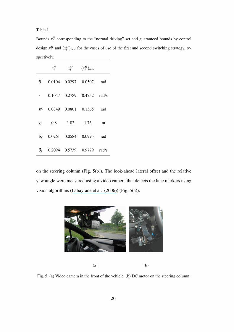
Table 1

Bounds xNi corresponding to the “normal driving” set and guaranteed bounds by control

design xMi and (xM

i )new for the cases of use of the first and second switching strategy, re-

spectively.

xNi xM

i (xMi )new

β 0.0104 0.0297 0.0507 rad

r 0.1047 0.2789 0.4752 rad/s

ψL 0.0349 0.0801 0.1365 rad

yL 0.8 1.02 1.73 m

δ f 0.0261 0.0584 0.0995 rad

δ f 0.2094 0.5739 0.9779 rad/s

on the steering column (Fig. 5(b)). The look-ahead lateral offset and the relative

yaw angle were measured using a video camera that detects the lane markers using

vision algorithms (Labayrade et al. (2006)) (Fig. 5(a)).

(a) (b)

Fig. 5. (a) Video camera in the front of the vehicle. (b) DC motor on the steering column.

20

6.3 Practical implementation results

To perform the tests, a segment of the test track with a road curvature less than

0.001m−1, which corresponds to a nearly straight road, was chosen. The driver

drove the instrumented vehicle following the center of the lane, occasionally taking

his hands off the steering wheel, or relaxing the steering control to simulate a lack

of attention (see Electronic Annex 1 in the online version of this article). The acti-

vation of the steering assistance was linked to a “beep” sound. Once the assistance

had been activated, the driver acted on the steering wheel after a few seconds to

recover the control of the vehicle.

Fig. 6 (a) shows the trajectories of the front wheels on the lane, as well as the limits

for the control activation at ±1.1m, the guaranteed overshoots limits at ±1.76m,

and the border of the lane at ±1.75m with respect to the center of the lane 6 . It

is apparent that after activation of the control system, the trajectories of the front

wheels did not cross the border of the lane. Moreover, they remained within the

normal driving zone, inside the ±1.1m lane strip. At the first reaction after the

system activation, the assistance system counter-steered using a torque of about

10Nm (see Fig. 6 (b)), and the trajectories of the front wheels occasionally crossed

the opposite line of the ±1.1m center strip. Subsequently, the vehicle was driven to

the center of the lane and experienced low frequency, small amplitude oscillations

around the centerline. The vehicle speed during the test varied between 18m/s and

6 In each figure that presents the test results, the assistance activation is represented by a

two-valued figure; the higher value corresponds to the situation in which the driver con-

trols the vehicle, while the lower value corresponds to the situation in which the assistance

system controls the vehicle. For better understanding, the two values are different for each

figure and are adapted to the figure scale.

21

22m/s.

Note that the assist torque represented in Fig. 6(b) is higher than the driver torque,

since in manual mode the driver is assisted by the motor itself, which works in this

mode as a classical electrically powered assistance (Electric Power Steering, EPS).

The driver torque is measured at the steering wheel, which is upstream of the EPS

multiplication factor. In Fig. 6(b) the driver’s torque is represented, and is not the

result of the driver’s torque multiplied by the EPS.

During the intervention of the assistance system, the electric motor provides the

necessary steering torque, which results from the control law. It was assumed that

during the assistance system intervention, the driver is not able to drive. The assis-

tance system takes over for the driver, but it is switched off as soon as the driver

recovers attention. Consequently, the driver feels the assistance acting on the steer-

ing wheel only during the moments of system deactivation. At these times, the

driver feels a small resistance in the steering wheel, which disappears quickly.

These results confirmed the expected performance, which is guaranteed by the con-

trol design method. In addition, it was noticed that the computed maximum bounds

are fairly conservative compared to the real data. This might be due to an over-

estimation of the polyhedron L(F) by the exterior ellipsoid εext . Consequently,

an important shortcoming of the above presented assistance system, the activation

conditions, could be improved. By intensive testing, it was noticed that the activa-

tion rules are sometimes too conservative and prevent the steering assistance from

switching on, as for example in Fig. 6 (a), at t = 112s. Therefore, section 7 presents

an alternative switching strategy.

22

(a) (b)

Fig. 6. (a) Trajectories of the front wheels (solid line), predefined lane strip ±d = ±1.1m

(solid line), computed driving lane strip ±dext = ±1.76m (dashed line), lane borders at

±1.75m (dash-dot line, this coincides with the previous dashed line), assistance activated

on 2 (first activation rules). (b) Driver’s torque (solid line), assistance torque (dash-dot line),

assistance activated on 5 (first activation rules).

7 Improving the switching strategy and new testing

7.1 New activation rules

In examining the activation/deactivation situations during the tests, it was noticed

that when slowly drifting out of the lane with a relatively small yaw angle and

yaw rate, the condition that the vehicle state still resides in the “normal driving”

zone is always satisfied when the vehicle leaves the ±d center lane strip. On the

contrary, for rapid lane departures, the steering assistance did not switch on because

the “normal driving” zone had previously been exceeded by the vehicle.

Hence, the developed control law was kept unchanged and the constraint x∈ L(FN)

was eliminated from the switching condition T 12r given in Eq. (11), while the con-

straint |Fx|= 1 (crossing of the±d center lane strip) was maintained. Nevertheless,

to satisfy some safety limits for the lateral displacement of the front wheels, a new

23

activation condition was added. It required that for any activation, the maximum

expected displacements of the front wheels dext(x) would be less than dext = 2.5m.

Taking into account the conservatism noticed in the experimental phase of the first

switching strategy, this value was chosen to be higher than the value corresponding

to the lane borders (1.75m). More specifically, for each state x for which the front

wheels reach the lane strip limits at ±d, the expected displacement dext(x) can be

computed by using Eq. (17) for Vext(x) = xT Px, as shown in Fig. 7. Moreover, the

guaranteed maximum bounds for the state variables during the control activation

were computed for the new ellipsoid εext related to dext = 2.5m, and are given in

Table 1, column (xMi )new.

In addition, the transition T 12r has to be triggered only if the vehicle is heading

towards a lane edge. This behavior might be characterized by a lateral offset and a

yaw angle that are simultaneously positive or negative.

For the deactivation of the steering assistance, the same conditions were used as in

the first switching strategy, in order to ensure safety when switching the system off

and the trajectory limits with respect to the switchings.

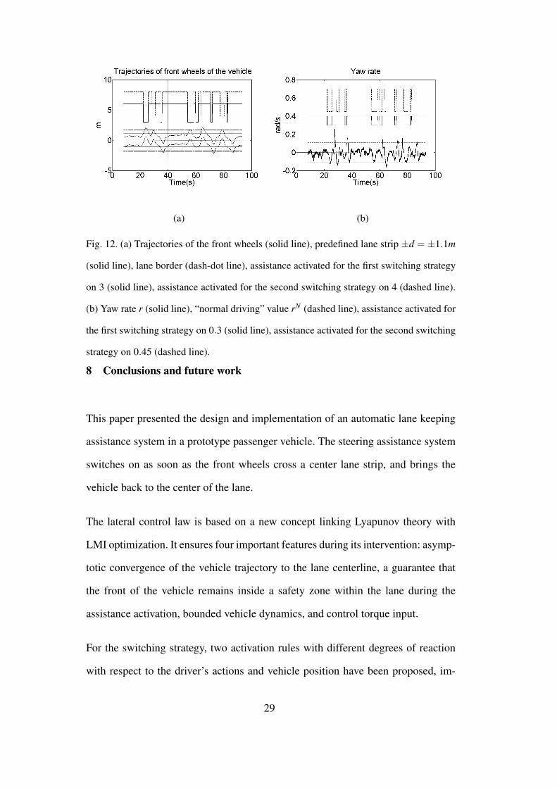
The proposed new switching strategy is illustrated in Fig. 7 and summarized in the

following logical equations:

T 12r : (|Td|< σ1)∧ (dext(x) < 2.5m)∧ (|Fx|= 1)∧ (ψL · yL) > 0). (23)

T 21r : [(σ1 ≤ |Td|< σ2)∧ (x ∈ (L(F))]∨ (|Td| ≥ σ2). (24)

24

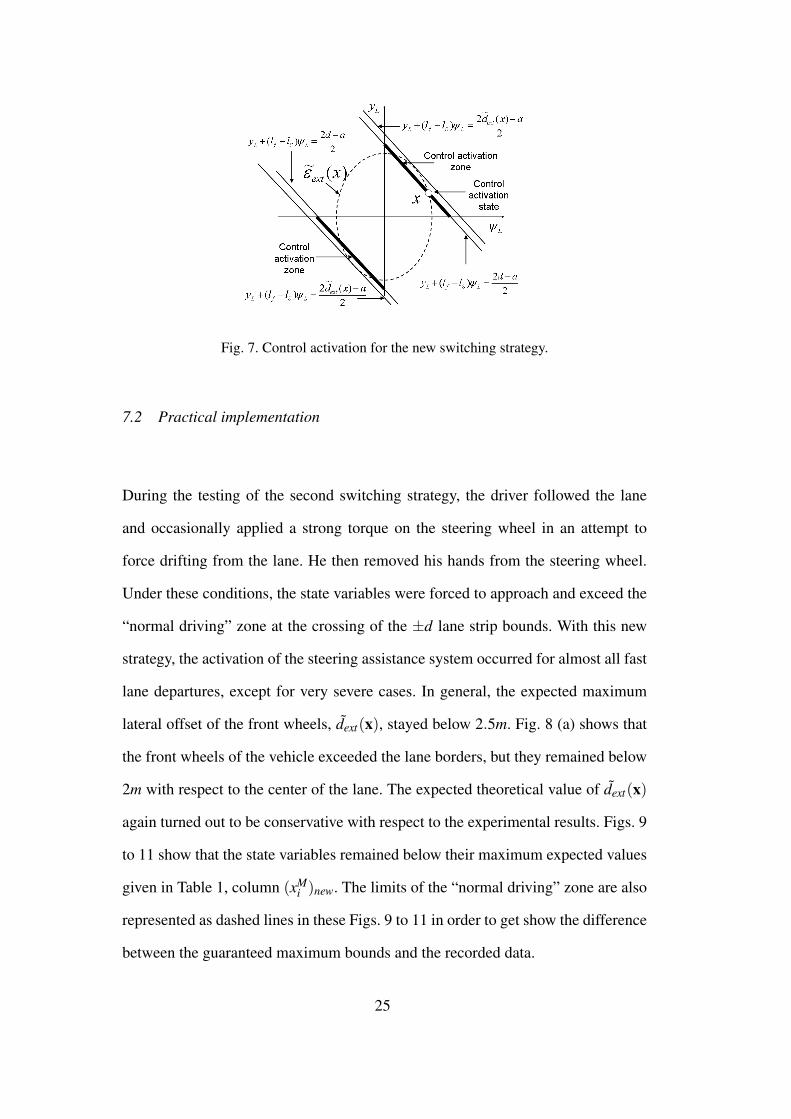
Fig. 7. Control activation for the new switching strategy.

7.2 Practical implementation

During the testing of the second switching strategy, the driver followed the lane

and occasionally applied a strong torque on the steering wheel in an attempt to

force drifting from the lane. He then removed his hands from the steering wheel.

Under these conditions, the state variables were forced to approach and exceed the

“normal driving” zone at the crossing of the ±d lane strip bounds. With this new

strategy, the activation of the steering assistance system occurred for almost all fast

lane departures, except for very severe cases. In general, the expected maximum

lateral offset of the front wheels, dext(x), stayed below 2.5m. Fig. 8 (a) shows that

the front wheels of the vehicle exceeded the lane borders, but they remained below

2m with respect to the center of the lane. The expected theoretical value of dext(x)

again turned out to be conservative with respect to the experimental results. Figs. 9

to 11 show that the state variables remained below their maximum expected values

given in Table 1, column (xMi )new. The limits of the “normal driving” zone are also

represented as dashed lines in these Figs. 9 to 11 in order to get show the difference

between the guaranteed maximum bounds and the recorded data.

25

(a) (b)

Fig. 8. (a) Trajectories of the front wheels (solid line), predefined lane strip ±d = ±1.1m

(solid line), lane border (dash-dot line), assistance activated on 2 (second activation rules).

(b) Driver torque (solid line), assistance torque (dash-dot line), assistance activated on 5

(second activation rules).

(a) (b)

Fig. 9. (a) Side slip angle β (solid line), “normal driving” value β N (dashed line), maximum

computed bound β M (dash-dot line), assistance activated on 0.03 (second activation rules).

(b) Yaw rate r (solid line), “normal driving” value rN (dashed line), maximum computed

bound rM (dash-dot line), assistance activated on 0.3 (second activation rules).

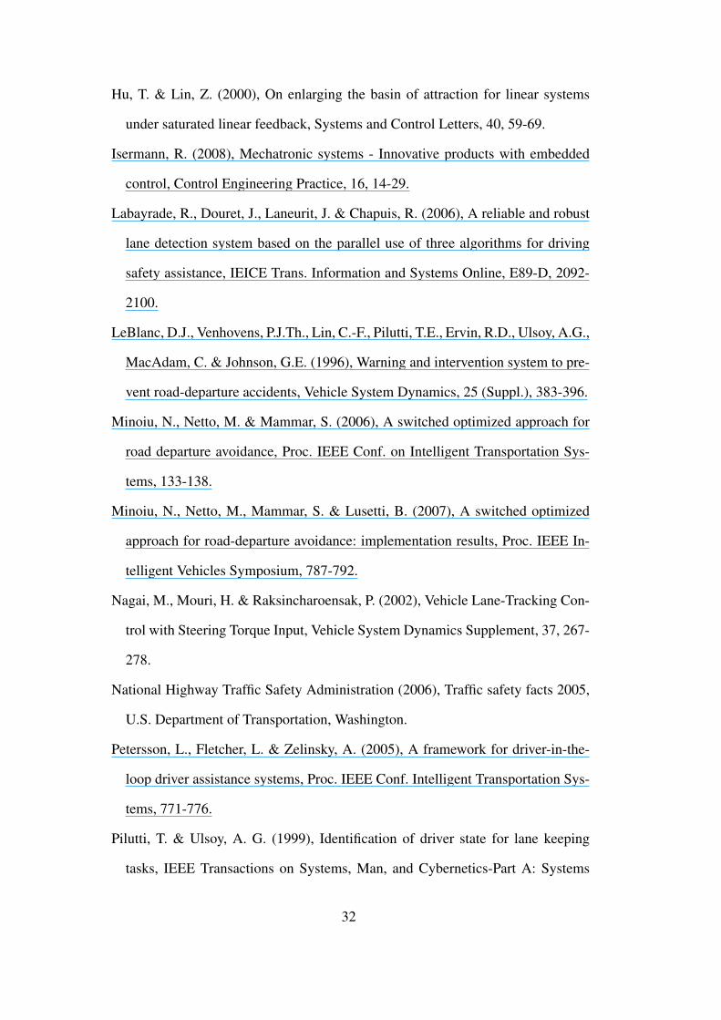
7.3 Comparison of the activation rules

In order to compare the activation of the two switching strategies, the following test

was performed. In the first stage, the equipped vehicle was driven on the test track

26

(a) (b)

Fig. 10. (a) Relative yaw angle ψL (solid line), “normal driving” value ψNL (dashed line),

maximum computed bound ψML (dash-dot line), assistance activated on 0.1 (second acti-

vation rules). (b) Lateral offset yL (solid line), “normal driving” value yNL (dashed line),

maximum computed bound yML (dash-dot line), assistance activated on 1 (second activation

rules).

(a) (b)

Fig. 11. (a) Steering angle δ f (solid line), “normal driving” value δ Nf (dashed line), maxi-

mum computed bound δ Mf (dash-dot line), assistance activated on 0.04 (second activation

rules). (b) Steering angle rate δ f (solid line), “normal driving” value δ Nf (dashed line), max-

imum computed bound δ Mf (dash-dot line), assistance activated on 0.05 (second activation

rules).

27

with the steering assistance system disabled, and it was allowed to leave the lane,

with the driver simulating a lack of attention. Subsequently, the vehicle trajectory

was corrected by the driver to the center of the lane, and the procedure was repeated

several times. All the variables necessary for the computation of the switching con-

ditions were recorded during the test. In the second stage, the activation conditions

were computed off-line for the two switching strategies, and were compared to

each other. The deactivation condition was reduced to a driver torque higher than

1.5Nm, to enforce a rapid deactivation of the system. The trajectories of the front

wheels are given in Fig. 12 (a). There are three cases of activation using the sec-

ond strategy in the absence of system activation using the first strategy. In all three

cases, the absence of the activation for the first switching strategy is due to a yaw

rate that exceeded its normal value rN (see Fig. 12 (b)). This result raises several

questions concerning the driving behavior during a “normal driving” situation and

the moment of loss of attention. As few statistical studies providing bounds of the

vehicle state variables during a usual lane keeping task are available, it is thus dif-

ficult to determine whether these missed activations for the first switching strategy

are dangerous or not.

To summarize, it can be noticed that with the two activation strategies of the steer-

ing assistance system, there is a place for calibrations and settings that take users’

opinions into account. The first activation conditions are more restrictive, but they

ensure a vehicle trajectory that is confined to the lane while remaining within com-

fortable and safe limits for the state variables during the control activation. The

second activation rules are more reactive and cover fast drifting from the lane, but

the danger to depart from the lane to collide with adjacent vehicles cannot be ex-

cluded.

28

(a) (b)

Fig. 12. (a) Trajectories of the front wheels (solid line), predefined lane strip ±d =±1.1m

(solid line), lane border (dash-dot line), assistance activated for the first switching strategy

on 3 (solid line), assistance activated for the second switching strategy on 4 (dashed line).

(b) Yaw rate r (solid line), “normal driving” value rN (dashed line), assistance activated for

the first switching strategy on 0.3 (solid line), assistance activated for the second switching

strategy on 0.45 (dashed line).

8 Conclusions and future work

This paper presented the design and implementation of an automatic lane keeping

assistance system in a prototype passenger vehicle. The steering assistance system

switches on as soon as the front wheels cross a center lane strip, and brings the

vehicle back to the center of the lane.

The lateral control law is based on a new concept linking Lyapunov theory with

LMI optimization. It ensures four important features during its intervention: asymp-

totic convergence of the vehicle trajectory to the lane centerline, a guarantee that

the front of the vehicle remains inside a safety zone within the lane during the

assistance activation, bounded vehicle dynamics, and control torque input.

For the switching strategy, two activation rules with different degrees of reaction

with respect to the driver’s actions and vehicle position have been proposed, im-

29

plemented on the prototype vehicle, and tested. Using both rules, unintended lane

departures are avoided, without leaving the lane in the first case and with a small

overshoot with respect to the lane borders in the second case. As a trade-off, the

second activation rule ensures better reactions for fast drifting out the lane.

In the future, we intend to perform an acceptance study of the proposed steering

assistance systems using test drivers. This study could be extended by a comple-

mentary statistical study concerning the limits of the vehicle dynamic variables

during “normal driving”, especially if the driver experiences moments of inatten-

tion. The topic of avoiding unintended lane departure for curvy roads is a topic of

current research.

References

Ackermann, J., Guldner, J., Sienel, W., Steinhauser, R. & Utkin, V. U. (1995), Lin-

ear and Nonlinear Controller Design for Robust Automatic Steering, IEEE Trans.

Control Systems Technology, 132-143.

Bar, F. & Page, Y. (2002), Les sorties de voie involontaires, CEESAR - LAB Tech.

Rep. ARCOS.

Blanchini, F. (1999), Set invariance in control, Automatica, 35, 1747-1767.

Boyd, S., El Ghaoui, L., Feron, E. & Balakrishnan, V. (1994), Linear Matrix In-

equalities in System and Control Theory, Society for Industrial and Applied

Mathematics, Philadelphia.

Bullock, D. & Zelek, J. (2005), Towards real-time 3-D monocular visual tracking of

human limbs in unconstrained environments, Real-Time Imaging, 11, 323-353.

Eidehall, A., Pohl, J. & Gustafsson, F. (2007), Joint road geometry estimation and

vehicle tracking, Control Engineering Practice, 15, 1484-1494.

30

Table 2

Values of the vehicle parameters.

Parameter Value

BS steering system damping coefficient 15

c f 0 front cornering stiffness 40000 N/rad

cr0 rear cornering stiffness 35000 N/rad

IS inertial moment of steering system 0.05 kg·m2

J vehicle yaw moment of inertia 2454 kg·m2

KP manual steering column coefficient 1

l f distance form CG to front axle 1.22 m

lr distance from CG to rear axle 1.44 m

lS look-ahead distance 0.95 m

a vehicle width 1.5 m

m total mass 1600 kg

RS steering gear ratio 14

v longitudinal velocity [18;22] m/s

ηt tire length contact 0.13 m

µ adhesion 1

L lane width 3.5 m

31

Hu, T. & Lin, Z. (2000), On enlarging the basin of attraction for linear systems

under saturated linear feedback, Systems and Control Letters, 40, 59-69.

Isermann, R. (2008), Mechatronic systems - Innovative products with embedded

control, Control Engineering Practice, 16, 14-29.

Labayrade, R., Douret, J., Laneurit, J. & Chapuis, R. (2006), A reliable and robust

lane detection system based on the parallel use of three algorithms for driving

safety assistance, IEICE Trans. Information and Systems Online, E89-D, 2092-

2100.

LeBlanc, D.J., Venhovens, P.J.Th., Lin, C.-F., Pilutti, T.E., Ervin, R.D., Ulsoy, A.G.,

MacAdam, C. & Johnson, G.E. (1996), Warning and intervention system to pre-

vent road-departure accidents, Vehicle System Dynamics, 25 (Suppl.), 383-396.

Minoiu, N., Netto, M. & Mammar, S. (2006), A switched optimized approach for

road departure avoidance, Proc. IEEE Conf. on Intelligent Transportation Sys-

tems, 133-138.

Minoiu, N., Netto, M., Mammar, S. & Lusetti, B. (2007), A switched optimized

approach for road-departure avoidance: implementation results, Proc. IEEE In-

telligent Vehicles Symposium, 787-792.

Nagai, M., Mouri, H. & Raksincharoensak, P. (2002), Vehicle Lane-Tracking Con-

trol with Steering Torque Input, Vehicle System Dynamics Supplement, 37, 267-

278.

National Highway Traffic Safety Administration (2006), Traffic safety facts 2005,

U.S. Department of Transportation, Washington.

Petersson, L., Fletcher, L. & Zelinsky, A. (2005), A framework for driver-in-the-

loop driver assistance systems, Proc. IEEE Conf. Intelligent Transportation Sys-

tems, 771-776.

Pilutti, T. & Ulsoy, A. G. (1999), Identification of driver state for lane keeping

tasks, IEEE Transactions on Systems, Man, and Cybernetics-Part A: Systems

32

and Humans, Vol. 29, No. 5, 486-502.

Pomerleau, D., Jochem, T., Thorpe, C., Batavia, P., Pape, D., Hadden, J., McMillan,

N., Brown, N. & Everson, J. (1999), Run-of-road collision avoidance using IVHS

countermeasures, U.S. Department of Transportation National Highway Traffic

Safety Administration, Technical Report DOT HS 809 170.

Rossetter, E. J., Switkes, J. P. & Gerdes, J. C. (2004), Experimental validation of

the potential field lanekeeping system, Int. Journal of Automotive Technology,

5, 95-108.

Raharijoana, T. (2004), Commande robuste pour l’assistance au controle lateral

d’un vehicule routier, PhD thesis, Universite Paris XI Orsay.

Shimakage, M., Satoh, S., Uenuma, K. & H. Mouri (2002), Design of lane-keeping

control with steering torque input, JSAE Review, 23, 317-323.

Stilwell, D.J. & Rugh, W. J. (1997), Interpolation of Observer State Feedback Con-

trollers for Gain Scheduling, IEEE Transaction on Automatic Control, 44, 1225-

1229.

Scherer, C., Gahinet, P. & Chilali, M. (1997), Multiobjective output-feedback con-

trol via LMI optimization, IEEE Transaction on Automatic Control, 42, 896-911.

33

List of Figures

1 Vehicle “bicycle” model. 6

2 Vehicle in the lane. 7

3 “Normal driving” zone represented in a two-dimensional state

space ((yL,ψL)). 9

4 The polyhedron L(F) and the ellipsoids ε and εext , represented in a

two-dimensional state space (yL, ψL). 13

5 (a) Video camera in the front of the vehicle. (b) DC motor on the

steering column. 20

6 (a) Trajectories of the front wheels (solid line), predefined lane

strip ±d = ±1.1m (solid line), computed driving lane strip

±dext =±1.76m (dashed line), lane borders at ±1.75m (dash-dot

line, this coincides with the previous dashed line), assistance

activated on 2 (first activation rules). (b) Driver’s torque (solid

line), assistance torque (dash-dot line), assistance activated on 5

(first activation rules). 22

7 Control activation for the new switching strategy. 24

8 (a) Trajectories of the front wheels (solid line), predefined lane

strip ±d = ±1.1m (solid line), lane border (dash-dot line),

assistance activated on 2 (second activation rules). (b) Driver

torque (solid line), assistance torque (dash-dot line), assistance

activated on 5 (second activation rules). 25

9 (a) Side slip angle β (solid line), “normal driving” value β N

(dashed line), maximum computed bound β M (dash-dot line),

assistance activated on 0.03 (second activation rules). (b) Yaw rate

r (solid line), “normal driving” value rN (dashed line), maximum

computed bound rM (dash-dot line), assistance activated on 0.3

(second activation rules). 26

10 (a) Relative yaw angle ψL (solid line), “normal driving” value ψNL

(dashed line), maximum computed bound ψML (dash-dot line),

assistance activated on 0.1 (second activation rules). (b) Lateral

offset yL (solid line), “normal driving” value yNL (dashed line),

maximum computed bound yML (dash-dot line), assistance activated

on 1 (second activation rules). 26

11 (a) Steering angle δ f (solid line), “normal driving” value δ Nf

(dashed line), maximum computed bound δ Mf (dash-dot line),

assistance activated on 0.04 (second activation rules). (b) Steering

angle rate δ f (solid line), “normal driving” value δ Nf (dashed

line), maximum computed bound δ Mf (dash-dot line), assistance

activated on 0.05 (second activation rules). 27

12 (a) Trajectories of the front wheels (solid line), predefined lane

strip ±d = ±1.1m (solid line), lane border (dash-dot line),

assistance activated for the first switching strategy on 3 (solid

line), assistance activated for the second switching strategy on 4

(dashed line). (b) Yaw rate r (solid line), “normal driving” value rN

(dashed line), assistance activated for the first switching strategy

on 0.3 (solid line), assistance activated for the second switching

strategy on 0.45 (dashed line). 28

List of Tables

1 Bounds xNi corresponding to the “normal driving” set and

guaranteed bounds by control design xMi and (xM

i )new for the cases

of use of the first and second switching strategy, respectively. 19

2 Values of the vehicle parameters. 30