HAL Id: hal-01593128 https://hal.archives-ouvertes.fr/hal-01593128 Preprint submitted on 25 Sep 2017 HAL is a multi-disciplinary open access archive for the deposit and dissemination of sci- entific research documents, whether they are pub- lished or not. The documents may come from teaching and research institutions in France or abroad, or from public or private research centers. L’archive ouverte pluridisciplinaire HAL, est destinée au dépôt et à la diffusion de documents scientifiques de niveau recherche, publiés ou non, émanant des établissements d’enseignement et de recherche français ou étrangers, des laboratoires publics ou privés. Drinfeld–Sokolov hierarchies, tau functions, and generalized Schur polynomials Mattia Cafasso, Ann Du Crest de Villeneuve, Di Yang To cite this version: Mattia Cafasso, Ann Du Crest de Villeneuve, Di Yang. Drinfeld–Sokolov hierarchies, tau functions, and generalized Schur polynomials. 2017. hal-01593128

Welcome message from author
This document is posted to help you gain knowledge. Please leave a comment to let me know what you think about it! Share it to your friends and learn new things together.
Transcript

HAL Id: hal-01593128https://hal.archives-ouvertes.fr/hal-01593128
Preprint submitted on 25 Sep 2017
HAL is a multi-disciplinary open accessarchive for the deposit and dissemination of sci-entific research documents, whether they are pub-lished or not. The documents may come fromteaching and research institutions in France orabroad, or from public or private research centers.
L’archive ouverte pluridisciplinaire HAL, estdestinée au dépôt et à la diffusion de documentsscientifiques de niveau recherche, publiés ou non,émanant des établissements d’enseignement et derecherche français ou étrangers, des laboratoirespublics ou privés.
Drinfeld–Sokolov hierarchies, tau functions, andgeneralized Schur polynomials
Mattia Cafasso, Ann Du Crest de Villeneuve, Di Yang
To cite this version:Mattia Cafasso, Ann Du Crest de Villeneuve, Di Yang. Drinfeld–Sokolov hierarchies, tau functions,and generalized Schur polynomials. 2017. �hal-01593128�

arX
iv:1
709.
0730
9v1
[m
ath-
ph]
21
Sep
2017
Drinfeld–Sokolov hierarchies, tau functions, andgeneralized Schur polynomials
Mattia Cafasso∗, Ann du Crest de Villeneuve∗, Di Yang†
∗ LAREMA, Universite d’Angers, 2 boulevard Lavoisier, Angers 49000, [email protected], [email protected]
† Max-Planck-Institut fur Mathematik, Vivatsgasse 7, Bonn 53111, [email protected]
Abstract
For a simple Lie algebra g and an irreducible faithful representation π of g, we introducethe Schur polynomials of (g, π)-type. We then derive the Sato–Zhou type formula fortau functions of the Drinfeld–Sokolov (DS) hierarchy of g-type. Namely, we show thatthe tau functions are linear combinations of the Schur polynomials of (g, π)-type with thecoefficients being the Plucker coordinates. As an application, we provide a way of computingpolynomial tau functions for the DS hierarchy. For g of low rank, we give several examplesof polynomial tau functions, and use them to detect bilinear equations for the DS hierarchy.
1 Introduction
Given a simple Lie algebra g over C, Drinfeld and Sokolov in [14] explained how to associate toit a family of commuting bi–hamiltonian PDEs known as the Drinfeld–Sokolov (DS) hierarchy ofg–type. Nowadays, Drinfeld–Sokolov hierarchies are certainly among the most studied examplesof integrable systems; one of their remarkable properties is that they are tau–symmetric [19,18, 36, 7], meaning that they admit the so-called tau function of an arbitrary solution to thehierarchy. For the case g = sln(C) the DS hierarchy of g-type coincides (under a particularchoice of the DS gauge [14, 2]) with the Gelfand–Dickey hierarchy, and so, in particular, forn = 2, with the celebrated Korteweg–de Vries (KdV) hierarchy. It is known that tau functionsof the Gelfand–Dickey hierarchies can be expressed as linear combinations of Schur polynomialswith the coefficients being Plucker coordinates1 [32, 38, 3, 30]. In this short paper we aimto generalize this fact to an arbitrary given Lie algebra g. The generalization will depend onmatrix realizations of g (note that the tau function itself is independent of the realizations of g[6]!). Indeed, one of our main observations is that the generalization of Schur polynomials areassociated to faithful representations.
1Indeed, more generally this is true for the KP hierarchy, of which the Gelfand–Dickey hierarchies are reduc-tions.
1

As an application of our result, we describe a systematic way of finding simple solutions (i.e.solutions whose tau function is a polynomial or a fractional power of it) of the DS hierarchy ofg-type. Of course, in the case of the hierarchies of type An, we recover the well-known results,since polynomial tau functions of these hierarchies (more generally of the KP hierarchy) hadbeen studied for many years, due to their relations with Backlund transformations [1] and thedynamical systems of Calogero type (see for instance [35] and the references therein). Moreover,it had been proved that the polynomial tau functions of the so–called BKP hierarchy can bewritten in terms of the projective representations of the symmetric group [37] and this hierarchy,moreover, contains as reductions some of the DS hierarchies of Dn-type, as explained in [12].Nevertheless, it seems to us that a systematic approach to the study of polynomial tau functionsassociated to the general case (i.e. for an arbitrary Lie algebra) is still missing, and this papergives a first result in this direction. The polynomial tau functions we obtain are, actually, quitenon–trivial, and can also be used to give some explicit information about the structure of thebilinear equations for the hierarchy.
In order to state precisely our results, we need to fix some notations about finite dimensionalLie algebras, loop algebras and Toeplitz determinants. Let g be a simple Lie algebra over C ofrank n, and h, h∨ the Coxeter and dual Coxeter numbers, respectively. Fix h a Cartan subalgebraof g. Take Π = {α1, . . . , αn} ⊂ h∗ a set of simple roots, and let △ ⊂ h∗ be the root system. Weknow that g has the root space decomposition
g = h⊕⊕
α∈△
gα.
Let θ denote the highest root with respect to Π, and (·|·) : g × g → C the normalized Cartan–Killing form, i.e. (θ|θ) = 2. For a root α ∈ △, denote by Hα the unique vector in h satisfying(Hα|Hβ) = (α|β), ∀ β ∈ △.
Let Ei ∈ gαi, Fi ∈ g−αi
, Hi = 2Hαi/(αi|αi) be a set of Weyl generators of g. They satisfy
[Ei, Fi] = Hi, [Hi, Ej] = Aij Ej, [Hi, Fj] = −Aij Fj, 1 ≤ i, j ≤ n,
where (Aij)ni,j=1 is the Cartan matrix of g. Choose E−θ ∈ g−θ, Eθ ∈ gθ, normalized by the
conditions (Eθ |E−θ) = 1 and ω(E−θ) = −Eθ, where ω : g → g is the Chevalley involution. LetI+ :=
∑ni=1Ei be a principal nilpotent element of g. Denote by L(g) = g ⊗ C[λ, λ−1] the loop
algebra of g. On L(g) there is the principal gradation defined by assigning
degEi = 1, degHi = 0, deg Fi = −1, i = 1, . . . , n, deg λ = h
such that L(g) decomposes into homogeneous subspaces
L(g) =⊕
j∈Z
L(g)j .
Here, elements in L(g)j have degree j. Define Λ ∈ L(g) by
Λ = I+ + λE−θ. (1)
Clearly, Λ is homogeneous of degree 1. Denote by L(g)<0 elements in L(g) with negative degrees,similarly, by L(g)≤0 elements with non-positive degrees.
2

It was shown in [26, 29] that Ker adΛ ⊂ L(g) has the following decomposition
Ker adΛ =⊕
ℓ∈E
CΛℓ, deg Λℓ = ℓ ∈ E :=n⊔
i=1
(mi + hZ)
where the integers m1, . . . , mn are the exponents of g, and E is called the set of exponents ofL(g). We use E+ to denote the set of positive exponents. The elements Λi commute pairwise
[Λi,Λj] = 0, ∀ i, j ∈ E. (2)
They can be normalized by
Λma+kh = Λmaλk, k ∈ Z,
(Λma|Λmb
) = hλ δa+b,n+1.
In particular, we can choose Λ1 = Λ.
Let us now takeπ : g → gl(m,C) (3)
an irreducible faithful representation. When no confusion can arise, for b ∈ g, we write π(b)simply as b. Our generalization will be based on the infinite Grassmannian approach [32, 33] andthe related Plucker coordinates.
Notations:a) For M =
∑k∈Z Mk λ
k with Mk ∈ gl(m,C), define the Laurent matrix L(M) associated withM by
[L(M)]IJ = MI−J , I, J ∈ Z. (4)
Here, capital-letter indices I, J,K, . . . are used for block row/column coordinates, and small-letter indices are for ordinary row/column coordinates.b) Y will denote the set of all partitions; for λ = (λ1 ≥ λ2 ≥ . . . ) ∈ Y, ℓ(λ) denotes the length ofλ, |λ| the weight of λ; denote by λ = ( k1, . . . , kd | l1, . . . , ld ) be the Frobenius notation of λ withd being the Frobenius rank.
Definition 1.1. Let ξ :=∑
ℓ∈E+tℓ Λℓ with tℓ, ℓ ∈ E+ being indeterminates and let s denote the
Laurent matrix associated with eξ, namely,
s := L(eξ). (5)
The Schur polynomials of (g, π)-type are labelled by partitions and defined by
sλ := det(si−1, j−λj−1
)ℓ(λ)i,j=1
, λ ∈ Y− ∅,
s∅ := 1. (6)
Definition 1.2. In the case π is taken as the adjoint representation of g, we call sλ, λ ∈ Y theintrinsic Schur polynomials of g-type.
Remark 1.3. In the case g = An. Take π(g) the well-known matrix realization of g, i.e. π(g) =sln+1(C). We have Λ =
∑ni=1Ei,i−1+λE1,n+1. The Schur polynomials of (g, π)-type then coincide
with the Schur polynomials [30] under the restriction t(n+1)k ≡ 0, k = 1, 2, 3, . . . .
3

Definition 1.4. ∀X ∈ λ−1g[[λ−1]], denote by rX the Laurent matrix associated with eX , i.e.
rX := L(eX). (7)
For λ = (λ1, . . . , λℓ(λ)) ∈ Y, define
rX,λ := det (rX,i−λi−1,j−1)ℓ(λ)i,j=1 .
Definition 1.5. For ξ =∑
ℓ∈E+tℓ Λℓ (as above), and for any X ∈ λ−1g[[λ−1]], define matrices
DIJ and ZX,IJ (I, J ≥ 0) by
I − eξ(λ) e−ξ(µ)
λ− µ=
∞∑
I,J=0
DIJ λI+1µJ+1, (8)
I − eX(λ) e−X(µ)
λ− µ=
∞∑
I,J=0
ZX, IJ λ−I−1µ−J−1. (9)
Define s(i|j), r(i|j) (i, j ≥ 0) via
(DIJ)ab = sm·I+a−1,m·J+m−b,
(ZX, IJ)ab = rm·I+m−a,m·J+b−1
where a, b = 1, . . . , m. We call ZX, IJ the matrix-valued affine coordinates and rX, (i|j) the affinecoordinates.
Remark 1.6. The matrix-valued affine coordinates ZX, IJ and their generating formula (9) wereintroduced in [3] by F. Balogh and one of the authors of the present paper for the sl2(C) case.
The following theorem is the main result of the paper. Denote by κ the constant such that
(a|b) = κTr(π(a)π(b)) ∀a, b ∈ g. (10)
Theorem 1.7. For any X ∈ λ−1g[[λ−1]], the formal series τ defined by
τ :=
(∑
ν∈Y
rX,ν sν
)κ
(11)
is a tau function of the Drinfeld–Sokolov hierarchy of g-type. Moreover, sν and rX,ν have thefollowing expressions
sν = det(s(ki|lj)
)di,j=1
, (12)
rX,ν = (−1)l1+···+ld det(rX,(ki|lj)
)di,j=1
. (13)
We refer to (11)–(13) as the Sato–Zhou type formula for tau functions of the DS hierarchy.
4

Remark 1.8. As the reader might already have noticed, here the terminology is very similar to theone used to deal with the KP hierarchy in the Sato’s approach. However, it is worth mentioningthat tau functions of the DS hierarchies of g-type in general are not KP tau functions (except forg = sln+1(C)). One way to see it (which is close to the spirit of this paper) is that the generalizedSchur polynomials sν of (g, π)-type we defined are “reductions” (in the sense of the Remark 1.3)of the usual ones [30] just in the An case.
Remark 1.9. The formula (11) is intrinsic when π is taken as the adjoint representation of g.We will study the intrinsic Schur polynomials associated to g in a future publication.
Remark 1.10. For the ABCD cases, a result similar to Theorem 1.7 was obtained in [39] wherea different method was used; see also in [4] for more details for the An case.
Organization of the paper In Section 2 we review the Drinfeld–Sokolov hierarchies and theirtau functions. In Section 3 we prove Theorem 1.7. Some explicit examples and applications aregiven in Section 4. A list of first few Schur polynomials of (g, π)-type for g of low ranks andparticular choices of π are given in the Appendix.
Acknowledgements We would like to thank Ferenc Balogh, Marco Bertola, Boris Dubrovin,John Harnad, Leonardo Patimo, Daniele Valeri, Chao-Zhong Wu and Jian Zhou for helpfuldiscussions. D.Y. is grateful to Youjin Zhang and Boris Dubrovin for their advisings, and toVictor Kac for helpful suggestions. Part of our work was done at SISSA; we acknowledge SISSAfor excellent working conditions and generous supports. A.D. and M.C. thank the Centre HenriLebesgue ANR-11-LABX-0020-01 for creating an attractive mathematical environment. Partof the work of D.Y. was done during his visits to LAREMA; he acknowledges the support ofLAREMA and warm hospitality.
2 Review of the Grassmannian approach to the DS hier-
archy
Denote by b the Borel subalgebra of g, i.e. b := g≤0, and by n the nilpotent subalgebra n := g<0.Define a linear operator L by
L := ∂x + Λ + q(x) (14)
where q(x) ∈ b. It is proved by V. G. Drinfeld and V. V. Sokolov [14] that there exists a uniquesmooth function U(x) ∈ g((λ−1))<0 ∩ Im adΛ such that
e−adU(x)L = ∂x + Λ +H(x), H(x) ∈ Ker adΛ.
The following commuting system of PDEs
∂L
∂tℓ= −
[(eadUΛℓ)≥0 , L
], ℓ ∈ E+ (15)
are called the pre-DS hierarchy of g-type.
5

Gauge transformations. For any smooth function N(x) ∈ n, the map
L 7→ L = eadNL = ∂x + Λ + q
is called a gauge transformation. A vector space V ⊂ g is called a DS gauge if it satisfies
[I+, n]⊕ V = b. (16)
Below we fix V a DS gauge. It was observed in [14] that the flows (15) can be reduced to gaugeequivalent classes; moreover, for any q(x) ∈ b, there exists a unique N(x) such that q(x) ∈ V .Let us denote
Lcan := ∂x + Λ + qcan(x), qcan(x) ∈ V.
Take v1, . . . , vn a homogeneous basis of V , namely deg vi = −mi, and write
qcan(x) =
n∑
i=1
ui(x) vi.
The DS hierarchy of g-type is defined as the system of the pre-DS flows for the complete setof representatives (aka gauge invariants) u1, . . . , un. Clearly, the precise form2 of this integrablehierarchy depends on the choice of the DS gauge V ; the hierarchies under different choices of Vare Miura equivalent [?, 24, 25, 19, 6]. We remark that a unified algorithm of writing the DShierarchy of g-type for an arbitrary choice V was obtained recently in [6]; it has the form
∂ui
∂tℓ= aiℓ[u
1, . . . , un], ℓ ∈ E+ (17)
where ai,ℓ[u1, . . . , un] are differential polynomials of u1, . . . , un. It should also be noted that for
the DS hierarchy of g-type the time variable t1 can be identified with −x.
The hierarchy (17) is known to be Hamiltonian and tau-symmetric [19, 24, 36, 7]. Therefore,for an arbitrary solution qcan of (17), there exists a tau function τ(t) of qcan. The tau function isdetermined up to a multiplicative factor of the form
exp(∑
ℓ∈E+
cℓ tℓ
)
where cℓ are arbitrary constants. We review in this subsection the Grassmannian approach totau functions.
Denote E = Cm where m is defined in (3). Let H := E((λ−1)) be the linear space of E-valuedformal series in z with finitely many positive powers and let H+ := E[z]. Denote by Gr theSato–Segal–Wilson Grassmannian [32, 33]. A point W ∈ Gr is a subspace of H . Here we areinterested in the big cell Gr(0) ⊂ Gr which consists of points W of the form
W = SpanC
{ei λ
ℓ +∑
k≥0
Ak,ℓ,i ei λ−k−1
}
i=1,...,m, ℓ≥0
.
Here Ak,ℓ,i are called the affine coordinates [20] of W .
2It also depends on scalings of the basis vi which gives rise to scalings of ui. Such a coordinate change is trivial(In the case g = Deven other linear transformation of ui needs to be considered but is again trivial).
6

Definition 2.1. Define Gr(0)g as the following subset of the big cell Gr(0)
Gr(0)g ={eaH+ | a ∈ λ−1g[[λ−1]]
}.
We call Gr(0)g the embedded big cell of g-type.
For a ∈ λ−1g[[λ−1]], write G = ea =∑
k≥0Gkλ−k. The matrices G0, G1, . . . serve as the
matrix-valued coordinates for the point W corresponding to a; see Fig. 1. Clearly, G0 = I.
...... . .
.
· · ·
· · ·
· · ·
· · ·
. . .
G2
G1
G0
G3
G2
G1
G0
Figure 1: Matrix-valued coordinates in Sato–Segal–Wilson Grassmannian
Definition 2.2. ∀M =∑
k∈Z Mk λk, Mk ∈ gl(m,C), the N-th (N ≥ 0) block Toeplitz matrix
associated to M is defined byTN (M) = (MI−J)
NI,J=0.
The following theorem comes from the results obtained in [9, 10].
Theorem A. (Cafasso–Wu [9, 10]) For any X ∈ λ−1g[[λ−1]], let γ = eξeX . Define τ = τ(t) by
τ =[lim
N→∞det TN (γ)
]κ, (18)
where κ is defined in (10). Then τ is a tau function of the DS hierarchy associated to g.
Remark 2.3. The stabilization proved in [22] for the case of the Witten–Kontsevich tau functionand extended in [10] for the general cases ensures that the limit in (18) is meaningful.
3 Proof of Theorem 1.7
Define γ = eξeX , where we recall that X is the given element in λ−1g[[λ−1]], and ξ =∑
ℓ∈E+tℓ Λℓ.
We haveL(γ) = L(eξ)L(eX) = s rX
7

where s, rX are defined in (5), (7), respectively. For any N ≥ 1, define two matrices
sN = (sN , ij)i∈{0,...,N}, j∈{−N−1,...,N}
andrN = (rN , ij)i∈{−N−1,...,N}, j∈{0,...,N}
bysN, ij := L(eξ)ij, rN, ij := L(eX)ij .
Then we havelim
N→∞det TN(γ) = lim
N→∞det(sN rN).
By using the well-known Cauchy–Binet formula (see for instance [21]) we obtain [32, 20] fromTheorem A that
τ 1/κ =∑
λ∈Y
rX,λ sλ
where we recall that rX,λ and sλ are defined by
rX,λ = det (ri−λi−1,j−1)ℓ(λ)i,j=1
andsλ = det
(si−1,j−λj−1
)ℓ(λ)i,j=1
.
As explained in [3], formulae (8) and (9) give the Gaussian eliminations and formulae (12)and (13) are due to the Giambelli-type formula [20, 30, 3]. The theorem is proved.
4 Polynomial tau functions and bilinear equations
Theorem 1.7 gives a simple procedure to compute the tau function τ when τ 1/κ is a polynomial.Indeed, let us fix the Lie algebra g and take a faithful representation π. Choosing X ∈ λ−1g[[λ−1]]such that π(X) is a nilpotent matrix, the infinite series in (11) becomes finite, as it is easy toverify that only finitely many Plucker coordinates {rµ, µ ∈ Y} are non zero. Consequently, τ 1/κ
is polynomial. This simple idea was used for example in [3] for the KdV hierarchy. If κ = 1,then the tau function itself is a polynomial. Interestingly enough, in the computations we willperform, even when κ = 1/2, we obtain some polynomial tau functions: in other words, the finitesum in (11) is a perfect square. Even if this result has not been proved in general, we expect thatour procedure gives a systematic way to compute all the polynomials tau functions (up to a shiftof the time variables {ti, i ∈ E+}) of the DS hierarchy of g-type. As stated in the introductionof [28], this is an interesting open problem.
In what follows we compute the first few polynomial tau functions of the DS hierarchy ofg-type for g = A1, A2, B2 and D4. We use these particular tau functions to deduce possiblebilinear equations of small degrees. Note that each Drinfeld–Sokolov hierarchy has infinitelymany solutions. The usual question is to find particular solutions to the DS hierarchy (solve allPDEs in this hierarchy together). Here we consider the inverse:
Deduce possible PDEs from particular solutions.
8

Sometimes, one particular solution already contains all the information of an equation andof the whole hierarchy. For example, the “topological solution” was used by B. Dubrovin andY. Zhang to construct the integrable hierarchy of topological type [19, 17]. However, a polynomialtau function τpoly of the DS hierarchy contains less information, namely, if τpoly satisfies somePDE, it will not guarantee directly that other tau functions of the DS hierarchy satisfy this PDE.Nevertheless, if τpoly does not satisfy a PDE, then the PDE cannot belong to the DS hierarchy.
4.1 Bilinear derivatives
Given two smooth functions f(x), g(x) with independent variables x = (xi)i∈I , where I denotesan index set. The bilinear derivatives Di1 · · ·Dik are operators defined via the identity
e∑
i∈I hi Di(f, g) ≡ f(x+ h) g(x− h), ∀h.
It means that, expanding both sides of this identity in h
e∑
i∈I hi Di(f, g) = (f, g) +∑
i∈I
hi Di(f, g) +∑
i,j∈I
hihj
2DiDj(f, g) + · · · ,
f(x+ h) g(x− h) = f(x)g(x) +∑
i∈I
hi
( ∂f∂xi
g − f∂g
∂xi
)+ · · ·
and comparing the coefficients of monomials of h, we obtain, for example,
Di(f, g) =∂f
∂xi
g − f∂g
∂xi
,
DiDj(f, g) =∂2f
∂xi∂xj
g + f∂2g
∂xi∂xj
−∂f
∂xi
∂g
∂xj
−∂f
∂xj
∂g
∂xi
.
For the Drinfeld–Sokolov hierarchy of g-type, we take I := E+. There is a natural gradationfor the bilinear derivatives, defined by assigning degDi = i for i ∈ E+. Denote by Hg thelinear space of bilinear equations satisfied by the Drinfeld–Sokolov hierarchies of g-type, whichdecomposes into homogeneous subspaces
Hg =⊕
i
H[i]g .
The gradation allows us to list all possible bilinear equations up to certain degree.
4.2 Examples of polynomial tau functions
4.2.1 The A1 case
Let us chose the standard matrix realization g = sl(2;C). Consider the following two elementsin λ−1g[[λ−1]]
1
λF =
1
λ
(0 01 0
),
1
λE =
1
λ
(0 10 0
). (19)
9

The associated polynomial tau functions are
τ1 = 1 + t1, τ2 = 1 + t3 −t313
(20)
respectively. Similarly, one computes polynomial tau functions corresponding to elements of theform λ−kF , λ−kE, k ≥ 2. For example, for k = 2, we obtain
τ3 = 1 + 2t3 − t5t1 + t23 +t313+
1
3t3t
31 −
1
45t61, (21)
τ4 = 1− t3t7 + 2t5 + t25 + t33t1 − t3t5t21 − t3t
21 +
1
3t7t
31 −
t5115
−1
15t5t
51 +
1
105t3t
71 −
t1014725
, (22)
corresponding to λ−2F and λ−2E, respectively.
Now consider all bilinear equations up to degree 4:
(β + α0D21 + α1D
41 + α2D1D3)(τ, τ) = 0 (23)
where β, α0, α1, α2 are complex constants. Requiring that τ1, τ2 satisfy the above ansatz (23), wefind that up to a multiplicative constant there is only one possible choice of coefficients:
(D41 − 4D1D3)(τ, τ) = 0. (24)
Similarly up to degree 6, we find out only two more possible linearly independent bilinear equa-tions that are satisfied by τ1, τ2, τ3, τ4
(D61 + 20D3
1D3 − 96D1D5)(τ, τ) = 0, (25)
(D31D3 + 2D2
3 − 6D1D5)(τ, τ) = 0, (26)
which are well known to belong to the hierarchy of A1-type, that is the KdV hierarchy. Conse-quently, we have shown that
dimC H[deg≤6]A1
≤ 3.
Moreover, (24)–(26) are the three only possible choices of homogeneous basis (up to constant
factors) of H[deg≤6]g .
Relation with the Adler–Moser polynomials. An alternative way of computing polynomialtau functions for the KdV hierarchy was given by Adler and Moser [1]. Define a family ofpolynomials θk(x = q1, q3, q5, . . . , q2k−1), k ≥ 0 recursively by
θ0 = 1, θ1 = x,
θ′k+1θk−1 + θk+1θ′k−1 = (2k − 1)θ2k, ∀ k ≥ 2,
where the prime denotes the x-derivative and for each k ≥ 2 the integration constant is chosento be q2k−1. The polynomials θk are known as the Adler–Moser polynomials. It was also provenin [1] that there exists a unique change of variables q → t that transforms the Adler–Moserpolynomials into the polynomial tau functions of the KdV hierarychy. In [15], one of the authorsof the present paper proved that the desired change of variables is given by q1 = t1 = x and
∑
i≥2
q2i−1
α2i−1z2i−1 = tanh
(∑
i≥2
t2i−1z2i−1
),
where α2i−1 := (−1)i−132 · · · (2i− 3)2(2i− 1). Up to a shift and renormalisation of the times, werecover in particular the polynomials given in equations (20)–(22).
10
4.2.2 The A2 case
We still chose the standard matrix realization g = sl(3;C). Consider for example the followingtwo elements in λ−1g[[λ−1]] :
X1 =1
λ
0 0 0a1 0 0a2 a3 0
, X2 =1
λ
0 a1 a20 0 a30 0 0
, (27)
where a1, a2, a3 are arbitrary constants. The corresponding polynomial tau functions will bedenoted by τ1, τ2, respectively. We have
τ1 = 1 + a2t1 +1
2a1t
2
1−
1
2a3t
2
1+
1
8a1a3t
4
1−
1
160a2
1a3t
6
1+
1
160a1a
2
3t6
1−
a2
1a2
3t81
1792+ a1t2 + a3t2 +
1
16a2
1a3t
4
1t2
+1
16a1a
2
3t4
1t2 +
3
2a1a3t
2
2−
1
8a2
1a3t
2
1t2
2+
1
8a1a
2
3t2
1t2
2+
1
32a2
1a2
3t4
1t2
2+
1
4a2
1a3t
3
2+
1
4a1a
2
3t3
2+
1
16a2
1a2
3t4
2−
1
4a2
1a3t
2
1t4
−1
4a1a
2
3t2
1t4 −
1
2a2
1a3t2t4 +
1
2a1a
2
3t2t4 −
1
4a2
1a2
3t2
1t2t4 −
1
4a2
1a2
3t2
4+
1
2a2
1a3t1t5 −
1
2a1a
2
3t1t5 +
1
4a2
1a2
3t1t7 ,
τ2 = 1−1
8a1t
4
1+
1
8a3t
4
1+
1
20a2t
5
1+
1
640a1a3t
8
1−
a2
1a3t
12
1
358400+
a1a2
3t121
358400−
a2
1a2
3t161
90112000−
1
2a1t
2
1t2 −
1
2a3t
2
1t2 −
a2
1a3t
10
1t2
12800−
a1a2
3t101
t2
12800+
1
2a1t
2
2−
1
2a3t
2
2
− a2t1t2
2+
1
16a1a3t
4
1t2
2−
13a2
1a3t
8
1t22
17920+
13a1a2
3t81t22
17920+
3a2
1a2
3t121
t22
1126400−
1
320a2
1a3t
6
1t3
2−
1
320a1a
2
3t6
1t3
2−
3
8a1a3t
4
2−
1
128a2
1a3t
4
1t4
2+
1
128a1a
2
3t4
1t4
2
−a2
1a2
3t81t42
10240−
1
32a2
1a3t
2
1t5
2−
1
32a1a
2
3t2
1t5
2−
1
32a2
1a3t
6
2+
1
32a1a
2
3t6
2+
1
256a2
1a2
3t4
1t6
2+
1
256a2
1a2
3t8
2+ a1t4 + a3t4 +
a2
1a3t
8
1t4
1280+
a1a2
3t81t4
1280
−3
2a1a3t
2
1t2t4+
1
160a2
1a3t
6
1t2t4−
1
160a1a
2
3t6
1t2t4−
a2
1a2
3t101
t2t4
12800+
1
32a2
1a3t
4
1t2
2t4+
1
32a1a
2
3t4
1t2
2t4−
1
8a2
1a3t
2
1t3
2t4+
1
8a1a
2
3t2
1t3
2t4−
1
320a2
1a2
3t6
1t3
2t4
−3
16a2
1a3t
4
2t4 −
3
16a1a
2
3t4
2t4 −
1
32a2
1a2
3t2
1t5
2t4 +
3
2a1a3t
2
4+
1
32a2
1a3t
4
1t2
4−
1
32a1a
2
3t4
1t2
4+
a2
1a2
3t81t24
2560−
3
8a2
1a3t
2
1t2t
2
4−
3
8a1a
2
3t2
1t2t
2
4−
1
8a2
1a3t
2
2t2
4
+1
8a1a
2
3t2
2t2
4+
1
64a2
1a2
3t4
1t2
2t2
4−
3
32a2
1a2
3t4
2t2
4+
1
4a2
1a3t
3
4+
1
4a1a
2
3t3
4−
1
8a2
1a2
3t2
1t2t
3
4+
1
16a2
1a2
3t4
4+ a2t5 +
1
2a1a3t
3
1t5 +
3a2
1a3t
7
1t5
1120−
3a1a2
3t71t5
1120
+a2
1a2
3t111
t5
140800+
1
80a2
1a3t
5
1t2t5 +
1
80a1a
2
3t5
1t2t5 +
1
8a2
1a3t
3
1t2
2t5 −
1
8a1a
2
3t3
1t2
2t5 +
1
320a2
1a2
3t7
1t2
2t5 +
1
4a2
1a3t1t
3
2t5 +
1
4a1a
2
3t1t
3
2t5 −
1
32a2
1a2
3t3
1t4
2t5
+1
4a2
1a3t
3
1t4t5 +
1
4a1a
2
3t3
1t4t5 −
1
2a2
1a3t1t2t4t5 +
1
2a1a
2
3t1t2t4t5 +
1
80a2
1a2
3t5
1t2t4t5 +
1
4a2
1a2
3t1t
3
2t4t5 +
1
8a2
1a2
3t3
1t2
4t5 +
1
4a2
1a3t
2
1t2
5−
1
4a1a
2
3t2
1t2
5
−1
160a2
1a2
3t6
1t2
5−
1
2a2
1a3t2t
2
5−
1
2a1a
2
3t2t
2
5−
1
8a2
1a2
3t2
1t2
2t2
5−
1
2a2
1a2
3t2t4t
2
5−
1
4a2
1a2
3t1t
3
5−
1
40a2
1a3t
5
1t7 +
1
40a1a
2
3t5
1t7 +
1
2a2
1a3t1t
2
2t7 −
1
2a1a
2
3t1t
2
2t7
−1
2a2
1a3t5t7 +
1
2a1a
2
3t5t7 −
1
16a2
1a3t
4
1t8 −
1
16a1a
2
3t4
1t8 −
1
4a2
1a3t
2
1t2t8 +
1
4a1a
2
3t2
1t2t8 −
1
160a2
1a2
3t6
1t2t8 +
1
4a2
1a3t
2
2t8 +
1
4a1a
2
3t2
2t8 +
1
8a2
1a2
3t2
1t3
2t8
+1
2a2
1a3t4t8 −
1
2a1a
2
3t4t8 −
1
16a2
1a2
3t4
1t4t8 +
1
4a2
1a2
3t2
2t4t8 +
1
2a2
1a2
3t1t2t5t8 −
1
4a2
1a2
3t2
8+
1
80a2
1a2
3t5
1t11 −
1
4a2
1a2
3t1t
2
2t11 +
1
4a2
1a2
3t5t11 .
Consider all possible bilinear equations of degree 4:
(α1D41 + α2D
22)(τ, τ) = 0,
Requiring τ1 satisfies this ansatz we find that there is only one possible choice:
(D41 + 3D2
2)(τ, τ) = 0.
Similarly, requiring that τ1 and τ2 to both satisfy the ansatz of bilinear equation of degree 6, wefind that there are only two linearly independent bilinear equations of degree 6:
(D61 + 45D2
1D22 + 90D2D4 − 216D1D5)(τ, τ) = 0,
(D61 + 15D2
1D22 + 60D2D4 − 96D1D5)(τ, τ) = 0,
which are well known to belong to the hierarchy of A2-type (i.e. the Boussinesq hierarchy).
11

4.2.3 The B2 case
We chose the matrix realization of the B2 simple Lie algebra as in [14]. We consider two explicitexamples given respectively by the following matrices3
X1 =1
λ
0 0 0 0 0a2 0 0 0 0a3 a5 0 0 0a4 0 a5 0 00 a4 −a3 a2 0
, X2 =1
λ
0 0 a3 a4 00 0 0 0 a40 0 0 0 −a30 0 0 0 00 0 0 0 0
.
The associated tau functions will be denoted by τ1 and τ2. They have the expressions
τ1 = 1 +1
2a4t1 +
1
4a3t
2
1+
1
12a2t
3
1−
1
12a5t
3
1−
1
192a2
3t4
1+
1
96a2a4t
4
1+
1
192a3a5t
5
1+
a2a5t6
1
1920−
1
720a2
5t6
1−
a2a4a5t7
1
11520−
a2a3a5t8
1
53760−
a2
2a5t
9
1
483840
+a2a
2
5t91
1088640+
a2a4a2
5t101
3110400+
11a2a3a2
5t111
87091200+
43a2
2a2
5t121
2090188800−
79a2a3
5t121
2874009600−
37a2
2a3
5t151
1931334451200+
a2
2a4
5t181
115880067072000+
1
2a2t3 + a5t3 −
1
8a2
3t1t3
+1
4a2a4t1t3 +
1
8a3a5t
2
1t3 +
1
16a2a5t
3
1t3 −
1
24a2
5t3
1t3 +
1
192a2a4a5t
4
1t3 +
1
640a2a3a5t
5
1t3 +
a2
2a5t
6
1t3
3840−
a2a2
5t61t3
1080−
a2a4a2
5t71t3
34560−
a2a3a2
5t81t3
193536
−31a2
2a2
5t91t3
17418240+
11a2a3
5t91t3
8709120+
101a2
2a3
5t121
t3
22992076800−
29a2
2a4
5t151
t3
6437781504000+
3
4a2a5t
2
3+
1
4a2
5t2
3+
1
16a2a4a5t1t
2
3+
5
288a2a
2
5t3
1t2
3+
a2a4a2
5t41t23
1152+
7a2a3a2
5t51t23
23040
+a2
2a2
5t61t23
138240−
17a2a3
5t61t23
69120−
13a2
2a3
5t91t23
34836480+
a2
2a4
5t121
t23
2043740160+
1
16a2
2a5t
3
3+
11
36a2a
2
5t3
3+
1
144a2a4a
2
5t1t
3
3−
1
576a2a3a
2
5t2
1t3
3+
a2
2a2
5t31t33
3456+
7a2a3
5t31t33
1728
−11a2
2a3
5t61t33
414720−
a2
2a4
5t91t33
34836480+
25
576a2
2a2
5t4
3+
5
144a2a
3
5t4
3+
a2
2a3
5t31t43
3456−
a2
2a4
5t61t43
552960+
5
576a2
2a3
5t5
3+
a2
2a4
5t63
2304−
1
4a2a5t1t5 +
1
4a2
5t1t5 −
1
16a2a4a5t
2
1t5
−1
48a2a3a5t
3
1t5 −
1
192a2
2a5t
4
1t5 +
1
72a2a
2
5t4
1t5 +
a2a4a2
5t51t5
5760−
11a2a3a2
5t61t5
69120+
a2
2a2
5t71t5
483840+
41a2a3
5t71t5
483840−
a2
2a3
5t101
t5
17418240+
a2
2a4
5t131
t5
4379443200
−1
8a2a3a5t3t5 −
1
8a2
2a5t1t3t5 −
1
24a2a
2
5t1t3t5 −
1
48a2a4a
2
5t2
1t3t5 −
5
576a2a3a
2
5t3
1t3t5 −
a2
2a2
5t41t3t5
1152+
7a2a3
5t41t3t5
1152+
29a2
2a3
5t71t3t5
967680
−a2
2a4
5t101
t3t5
116121600−
1
24a2a3a
2
5t2
3t5 −
7
96a2
2a2
5t1t
2
3t5 −
1
48a2a
3
5t1t
2
3t5 +
a2
2a3
5t41t23t5
1152+
a2
2a4
5t71t23t5
258048−
11
576a2
2a3
5t1t
3
3t5 +
a2
2a4
5t41t33t5
9216−
1
768a2
2a4
5t1t
4
3t5
−1
24a2a4a
2
5t2
5−
1
32a2a3a
2
5t1t
2
5+
1
64a2
2a2
5t2
1t2
5−
1
96a2a
3
5t2
1t2
5−
a2
2a3
5t51t25
2304−
a2
2a4
5t81t25
1290240+
1
192a2
2a3
5t2
1t3t
2
5−
a2
2a4
5t51t3t
2
5
7680+
a2
2a4
5t31t35
2304−
1
192a2
2a4
5t3t
3
5
+1
8a2a3a5t1t7 +
1
16a2
2a5t
2
1t7 −
1
8a2a
2
5t2
1t7 +
1
288a2a3a
2
5t4
1t7 +
a2
2a2
5t51t7
1440−
1
640a2a
3
5t5
1t7 −
a2
2a3
5t81t7
967680−
a2
2a4
5t111
t7
87091200+
1
12a2a3a
2
5t1t3t7
+1
24a2
2a2
5t2
1t3t7 −
1
16a2a
3
5t2
1t3t7 −
a2
2a3
5t51t3t7
11520−
a2
2a4
5t81t3t7
1935360+
1
192a2
2a3
5t2
1t2
3t7 −
a2
2a4
5t51t23t7
46080+
a2
2a4
5t21t33t7
1152+
1
12a2
2a2
5t5t7 −
1
12a2a
3
5t5t7
+1
576a2
2a3
5t3
1t5t7 +
7a2
2a4
5t61t5t7
138240+
1
24a2
2a3
5t3t5t7 +
a2
2a4
5t31t3t5t7
1152+
1
96a2
2a4
5t2
3t5t7 +
1
192a2
2a4
5t1t
2
5t7 −
1
48a2
2a3
5t1t
2
7−
a2
2a4
5t41t27
2304−
1
96a2
2a4
5t1t3t
2
7,
τ2 = 1 +1
288a3t
6
1−
a4t7
1
2016−
a2
3t121
11612160−
1
12a3t
3
1t3 +
1
48a4t
4
1t3 −
a2
3t91t3
69120+
1
2a3t
2
3−
1
2a4t1t
2
3−
a2
3t61t23
1920
−1
48a2
3t3
1t3
3+
1
16a2
3t4
3+
a2
3t71t5
4032−
1
96a2
3t4
1t3t5 +
1
4a2
3t1t
2
3t5 + a4t7 +
1
160a2
3t5
1t7 −
1
2a2
3t5t7.
Consider all bilinear equations up to degree 4
(α0 + α1D21 + α2D
41 + α3D1D3)(τ, τ) = 0
where α0, . . . , α3 are constants. Requiring that τ1 satisfies this ansatz of bilinear equations wefind that there is no solution. Similarly, up to degree 8, we find that there are only two possiblehomogeneous equations (one is of degree 6 and the other is of degree 8). We arrive at
3X2 is not the most general upper triangular element of homogeneous degree −1, as in this case the taufunction is too big to be written.
12

Proposition 4.1. The following dimension estimates hold true
dimC H[deg≤4]B2
= 0, dimC H[deg≤6]B2
≤ 1, dimC H[deg≤8]B2
≤ 2.
Moreover, the only possible elements in H[deg≤8]B2
are linear combinations of
(D61 − 5D3
1D3 − 5D23 + 9D1D5)(τ,τ) = 0,
and(D8
1 + 7D51D3 − 35D2
1D23 − 21D3
1D5 − 42D3D5 + 90D1D7)(τ, τ) = 0.
Remark 4.2. As far as we know, explicit bilinear equations for the DS hierarchy of B2-typeare not pointed out in the literature, except that there is a super-variable version given in [28].However, the relationship between the super bilinear equations of Kac–Wakimoto [28] and the DShierarchy of B2-type is not known. Finding explicit generating series of bilinear equations for theDS hierarchy of B2-type remains an open question. It is also interesting to remark that the verysame equations are contained in [13], as the first two equations of the BKP hierarchy.
4.2.4 The D4 case
Take the matrix realization of g as in [14, 5]. Consider the particular point of the Sato Grass-mannian of D4-type given by
γ = 1 + λEθ.
We put t11 = 0. It follows from Theorem 1.7 that the corresponding tau function is given by
τ =(1−
1
2s(7|6) −
1
2s(6|7) −
1
4s(7,6|7,6)
) 12
where s(7,6|7,6) = s(7|7)s(6|6) − s(7|6)s(6|7), s(6|6) = s(7|7) = 0, and
s(6|7) = s(7|6) =t111
1900800−
1
480t5t
61 +
1
160t23t
51 +
1
120t23′t
51 +
1
80t3t3′t
51
−1
8t33t
21 −
1
4t3t
23′t
21 −
3
8t23t3′t
21 +
1
2t25t1 +
3
4t23t5 + t23′t5 +
3
2t3t3′t5.
(28)
Hence we have
τ = 1−1
2s(7|6) =1−
t1113801600
+1
960t5t
61 −
1
320t23t
51 −
1
240t23′t
51 −
1
160t3t3′t
51
+1
16t33t
21 +
1
8t3t
23′t
21 +
3
16t23t3′t
21 −
1
4t25t1 −
3
8t23t5 −
1
2t23′t5 −
3
4t3t3′t5.
Proposition 4.3. The following dimension estimates hold true
dimC H[deg≤4]D4
= 0, dimC H[deg≤6]D4
≤ 3.
Moreover, the only possible elements in H[deg≤6]D4
are linear combinations of
(2D31D3′ + 4D3D3′ − 3D2
3′)(τ, τ) = 0, (29)
(D31D3 − D3
1D3′ + D3D3′ − D23)(τ, τ) = 0, (30)
(D61 + 9D1D5 − 10D3
1D3 + 5D31D3′ − 5D3D3′)(τ, τ) = 0. (31)
13
Our last remark is that under the following linear change of time variables
∂t1 7→ 2−1/6∂T1 ,
∂t3 7→ 21/2∂T3 ,
∂t3′ 7→ 21/2∂T3 + 21/23−1/2∂T3′,
∂t5 7→ 27/6∂T5
the bilinear equations (29)–(31) in the new time variables T1, T3, T3′ , T5 coincide with those ofKac and Wakimoto [28]. Essentially speaking such a change of times is simply a renormalizationof flows.
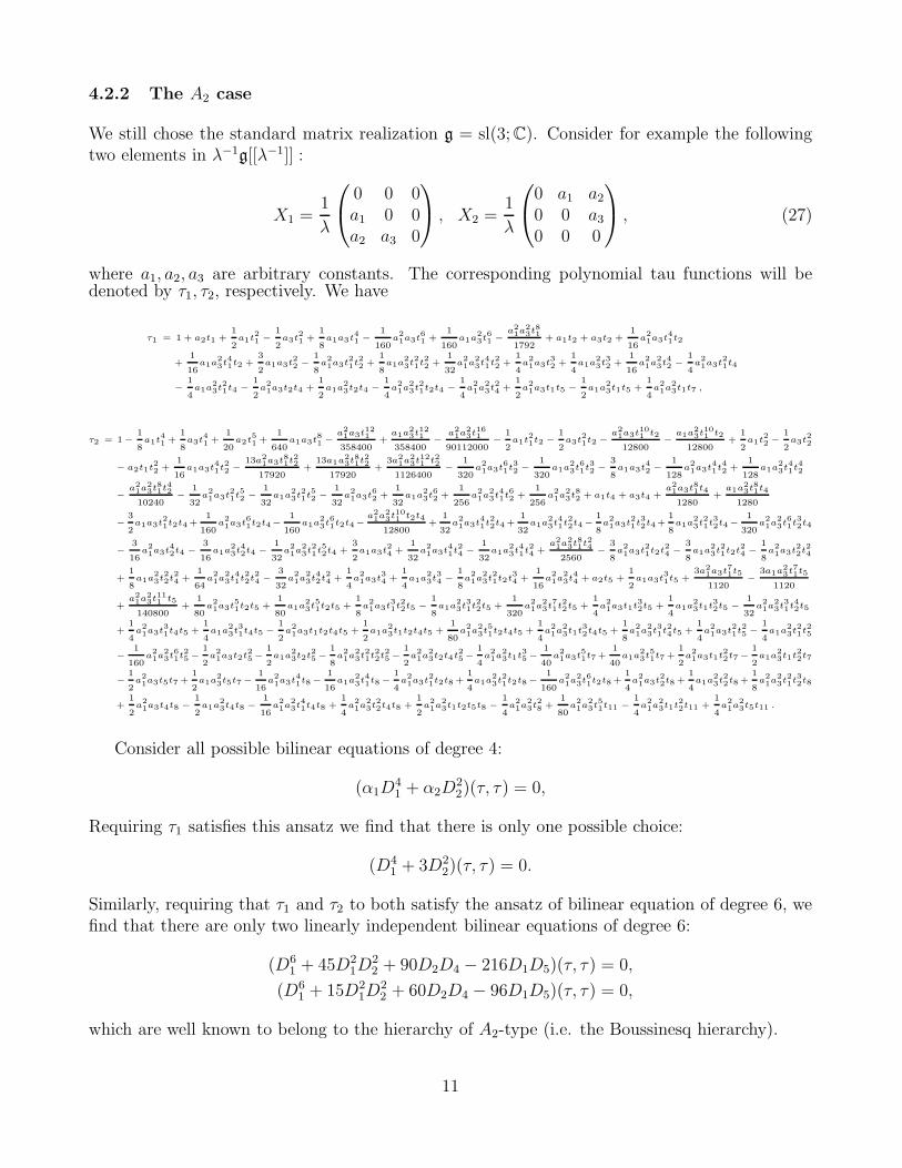
A List of generalized Schur polynomials of (g, π)-type
Take π as in [14, 10]. We list in Table 1 the first several Schur polynomials of (g, π)-type forsimple Lie algebras of low ranks.
g A1 A2 B2 B3 C2 D4
s1 t1 t1 0 0 t1 0
s212t21
12t21 + t2
12t1
12t1
12t21
12t1
s1212t21
12t21 − t2 −1
2t1 −1
2t1
12t21 −1
2t1
s316t31 + t3
16t31 + t1t2
14t21
14t21
13t31 + 2t3
14t21
s2113t31 − t3
13t31 0 0 1
3t31 − t3 0
s1316t31 + t3
16t31 − t1t2 −1
4t21 −1
4t21
13t31 + 2t3 −1
4t21
s4124t41 + t3t1
124t41+
12t2t
21+
12t22 + t4
112t31 +
12t3
112t31 +
12t3
112t41 +2t1t3
112t31 +
12t3 + t3′
s3118t41
18t41 +
12t21t2 −
12t22 − t4
112t31 − t3
112t31 − t3
14t41
112t31 − t3 −t3′
s22112t41 − t1t3
112t41 + t22
14t21
14t21
112t41 − t1t3
14t21
s21218t41
18t41 −
12t21t2 −
12t22 + t4
− 112t31 + t3 − 1
12t31 + t3
14t41
− 112t31 +
t3 + t3′
s14124t41 + t3t1
124t41−
12t2t
21+
12t22 − t4
− 112t31−
12t3 − 1
12t31−
12t3
112t41 +2t1t3
− 112t31 −
12t3 − t3′
Table 1: Simple Lie algebras and Schur polynomials of (g, π)-type
14

References
[1] Adler, M., Moser, J. (1978) On a class of polynomials connected with the Korteweg-de Vriesequation. Comm. Math. Phys. Volume 61, Number 1 (1978), 1-30.
[2] Balog, J., Feher, L., O’Raifeartaigh, L., Forgacs, P., Wipf, A. (1990). Toda theory andW-algebra from a gauged WZNW point of view. Annals of Physics, 203 (1), 76–136.
[3] Balogh, F., Yang, D. (2017). Geometric interpretation of Zhou’s explicit formula for theWitten–Kontsevich tau function. Lett. Math. Phys., doi: 10.1007/s11005-017-0965-8.
[4] Balogh, F., Yang, D., Zhou, J. Explicit formula for Witten’s r-spin partition function. toappear.
[5] Bertola, M., Dubrovin, B., Yang, D. (2016). Correlation functions of the KdV hierarchy andapplications to intersection numbers over Mg,n. Physica D: Nonlinear Phenomena, 327,30–57.
[6] Bertola, M., Dubrovin, B., Yang, D. (2016). Simple Lie algebras and topological ODEs.IMRN, rnw285.
[7] Bertola, M., Dubrovin, B., Yang, D. (2016). Simple Lie algebras, Drinfeld–Sokolov hierar-chies, and multi-point correlation functions. arXiv: 1610.07534.
[8] Cafasso, M. (2008). Block Toeplitz determinants, constrained KP and Gelfand-Dickey hier-archies, Math. Phys. Anal. Geom., 11 (1), 11–51.
[9] Cafasso, M., Wu, C.-Z. (2015). Tau functions and the limit of block Toeplitz determinants.IMRN, 2015 (20), 10339–10366.
[10] Cafasso, M., Wu, C.-Z. (2015). Borodin–Okounkov formula, string equation and topologicalsolutions of Drinfeld-Sokolov hierarchies. arXiv: 1505.00556v2.
[11] Cartan, E. (1894). Sur la structure des groupes de transformations finis et continus (Vol.826). Nony.
[12] Date, E., Jimbo, M., Kashiwara, M., Miwa, T. (1982). Transformation groups for solitonequations, Euclidean Lie algebras and reduction of the KP hierarchy. Publications of theResearch Institute for Mathematical Sciences, 18(3), 1077-1110.
[13] Date, E., Kashiwara, M., Miwa, T. (1981). Vertex operators and τ functions transformationgroups for soliton equations, II. Proceedings of the Japan Academy, Series A, MathematicalSciences, 57(8), 387-392.
[14] Drinfeld, V. G., Sokolov, V. V. (1985). Lie algebras and equations of Korteweg–de Vries type,J. Math. Sci. 30 (2), 1975–2036. Translated from Itogi Nauki i Tekhniki, Seriya SovremennyeProblemy Matematiki (Noveishie Dostizheniya) 24 (1984), 81–180.
[15] du Crest de Villeneuve, A. (2017). From the Adler–Moser polynomials to the polynomialtau functions of KdV. Preprint arXiv:1709.05632
15

[16] Dubrovin, B. (1996). Geometry of 2D topological field theories. In “Integrable Systems andQuantum Groups” (Montecatini Terme, 1993), Editors: Francaviglia, M., Greco, S.. SpringerLecture Notes in Math., 1620, 120–348.
[17] Dubrovin, B. (2014). Gromov–Witten invariants and integrable hierarchies of topologicaltype. In Topology, Geometry, Integrable Systems, and Mathematical Physics: Novikov’sSeminar 2012–2014, vol. 234, American Mathematical Soc.
[18] Dubrovin, B., Liu, S.-Q., Zhang, Y. (2008). Frobenius manifolds and central invariants forthe Drinfeld–Sokolov biHamiltonian structures. Advances in Mathematics, 219 (3), 780–837.
[19] Dubrovin, B., Zhang, Y. (2001). Normal forms of hierarchies of integrable PDEs, Frobeniusmanifolds and Gromov–Witten invariants. Preprint arXiv: math/0108160.
[20] Enolskii, V. Z., Harnad, J. (2011). Schur function expansions of KP τ -functions associatedto algebraic curves. Russian Mathematical Surveys, 66 (4), 767.
[21] Gantmacher, F. R. (2000). The Theory of Matrices, vols. I and II. AMS Chelsea Publishing,Providence R.I. (reprinted)
[22] Itzykson, C., Zuber, J.-B. (1992). Combinatorics of the modular group. II. The Kontsevichintegrals. Internat. J. Modern Phys. A, 7 (23), 5661–5705.
[23] Hirota, R. (2004). The Direct Method in Soliton Theory. Cambridge tracts in mathematics,155. Cambridge University Press.
[24] Hollowood, T., Miramontes, J. L. (1993). Tau-functions and generalized integrable hierar-chies. Comm. Math. Phys., 157 (1), 99–117.
[25] Hollowood, T. J., Miramontes, J., Guillen, J. S. (1994). Additional symmetries of generalizedintegrable hierarchies. Journal of Physics A: Mathematical and General, 27 (13), 4629.
[26] Kac, V. G. (1978). Infinite-dimensional algebras, Dedekind’s η-function, classical Mobiusfunction and the very strange formula. Advances in Mathematics, 30 (2), 85–136.
[27] Kac, V. G. (1994). Infinite-dimensional Lie algebras (Vol. 44). Cambridge University Press.
[28] Kac, V. G., Wakimoto, M. (1989). Exceptional hierarchies of soliton equations. In Proceed-ings of symposia in pure mathematics (Vol. 49, p. 191).
[29] Kostant, B. (1959). The Principal Three-Dimensional Subgroup and the Betti Numbers ofa Complex Simple Lie Group. American Journal of Mathematics, 973–1032.
[30] Macdonald, I. G. (1995). Symmetric functions and Hall polynomials. Second Edition. OxfordMathematical Monographs. Oxford University Press Inc., NewYork.
[31] Nimmo, J. J. C., Orlov, A. Y. (2005). A relationship between rational and multi-solitonsolutions of the BKP hierarchy. Glasgow Mathematical Journal, 47 (A), 149–168.
[32] Sato, M. (1981). Soliton Equations as Dynamical Systems on a Infinite Dimensional Grass-mann Manifolds (Random Systems and Dynamical Systems). RIMS Kokyuroku, 439, 30–46.
16

[33] Segal, G., Wilson, G. (1985). Loop groups and equations of KdV type. Inst. Hautes EtudesSci. Publ. Math., 61, 5–65.
[34] Shigyo, Y. (2016). On the expansion coefficients of Tau-function of the BKP hierarchy.Journal of Physics A: Mathematical and Theoretical, 49 (29), 295201.
[35] Wilson, G. (1998). Collisions of Calogero-Moser particles and an adelic Grassmannian. In-vent. math. 133, 1–41.
[36] Wu, C.-Z. (2012). Tau functions and Virasoro symmetries for Drinfeld-Sokolov hierarchies.Preprint arXiv: 1203.5750.
[37] You, Y. (1989). Polynomial solutions of the BKP hierarchy and projective representations ofsymmetric groups. Infinite-Dimensional Lie Algebras and Groups (Luminy-Marseille, 1988),Adv. Ser. Math. Phys, 7, 449-464.
[38] Zhou, J. (2013). Explicit formula for Witten-Kontsevich tau-function. arXiv: 1306.5429.
[39] Zhou, J. (2015). Fermionic Computations for Integrable Hierarchies. arXiv: 1508.01999.
17
Related Documents