Copyright © McDougal Littell/Houghton Mifflin Company. Georgia Notetaking Guide, Mathematics 2 255 7.1 Draw Scatter Plots and Best-Fitting Lines Goal p Fit lines to data in scatter plots. Georgia Performance Standard(s) MM2D2a, MM2D2b, MM2D2d Your Notes VOCABULARY Scatter plot Positive correlation Negative correlation Correlation coefficient Best-fitting line Linear regression Median-median line Algebraic model Inference

Welcome message from author
This document is posted to help you gain knowledge. Please leave a comment to let me know what you think about it! Share it to your friends and learn new things together.
Transcript
Copyright © McDougal Littell/Houghton Mifflin Company. Georgia Notetaking Guide, Mathematics 2 255
7.1 Draw Scatter Plots and Best-Fitting LinesGoal p Fit lines to data in scatter plots.Georgia
PerformanceStandard(s)
MM2D2a, MM2D2b, MM2D2d
Your Notes
VOCABULARY
Scatter plot
Positive correlation
Negative correlation
Correlation coefficient
Best-fitting line
Linear regression
Median-median line
Algebraic model
Inference
ga2nt-07.indd 152 4/16/07 9:04:03 AM
ga2_ntg_07.indd 255ga2_ntg_07.indd 255 4/19/07 3:47:05 PM4/19/07 3:47:05 PM

256 Georgia Notetaking Guide, Mathematics 2 Copyright © McDougal Littell/Houghton Mifflin Company.
Your Notes
Describe the data as having a positive correlation, a negative correlation, or approximately no correlation. Tell whether the correlation coefficient for the data is closest to 21, 20.5, 0, 0.5, or 1.
a.
x
y
1
1
b.
x
y
1
1
Solution
a. The scatter plot shows a strong correlation. So, the best estimate given is r 5 .
b. The scatter plot shows a weak correlation. So, r is between and , but not too close to either one. The best estimate given is r 5 .
Example 1 Describe and estimate correlation coefficients
1.
x
y
1
1
2.
x
y
1
1
Checkpoint For the scatter plot, (a) tell whether the data has a positive correlation, a negative correlation,or approximately no correlation, and (b) tell whether the correlation coefficient for the data is closest to 21, 20.5, 0, 0.5, or 1.
ga2nt-07.indd 153 4/16/07 9:04:04 AM
ga2_ntg_07.indd 256ga2_ntg_07.indd 256 4/19/07 3:47:07 PM4/19/07 3:47:07 PM

Copyright © McDougal Littell/Houghton Mifflin Company. Georgia Notetaking Guide, Mathematics 2 257
Your Notes
The table below gives the number of people y who attended each of the first seven football games x of the season. Approximate the best-fitting line for the data.
x 1 2 3 4 5 6 7
y 722 763 772 826 815 857 897
1. Draw a .
4 65 7
6500
700
750
800
850
900
x
y
Nu
mb
er
of
pe
op
le
Football game
2 310
2. Sketch the best-fitting line.
3. Choose two points on the line. For the scatter plot shown, you might choose (1, ) and (2, ).
4. Write an equation of the line. The line that passes through the two points has a slope of:
m 5 5
Use the point-slope form to write the equation.
y 2 y1 5 m(x 2 x1) Point-slope form
y 2 5 Substitute for m, x1, and y1.
y 5 Simplify.
An approximation of the best-fitting line is y 5 .
Example 2 Approximate the best-fitting line
3. The table gives the average class score y on each chapter test for the first six chapters x of the textbook.
x 1 2 3 4 5 6
y 84 83 86 88 87 90
a. Approximate the best-fitting line for the data.
b. Use your equation from part (a) to4 65
820
84
86
88
90
x
y
Ave
rag
e c
lass s
co
re
Test
2 310
predict the average class score on the chapter 9 test.
Checkpoint Complete the following exercise.
ga2nt-07.indd 154 4/16/07 9:04:05 AM
ga2_ntg_07.indd 257ga2_ntg_07.indd 257 4/19/07 3:47:08 PM4/19/07 3:47:08 PM
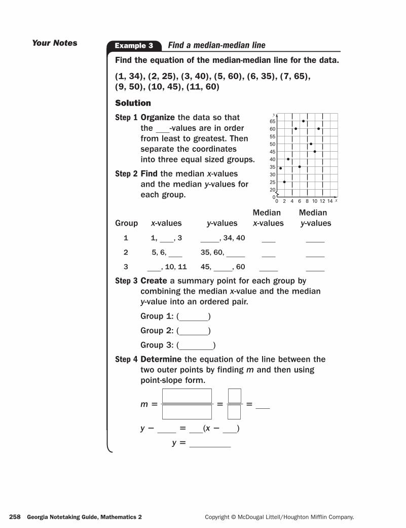
258 Georgia Notetaking Guide, Mathematics 2 Copyright © McDougal Littell/Houghton Mifflin Company.
Your Notes
Find the equation of the median-median line for the data.
(1, 34), (2, 25), (3, 40), (5, 60), (6, 35), (7, 65), (9, 50), (10, 45), (11, 60)
Solution
Step 1 Organize the data so that
8 1210 14
200
25
30
35
40
45
50
55
60
65
x
y
4 620
the -values are in order from least to greatest. Then separate the coordinates into three equal sized groups.
Step 2 Find the median x-valuesand the median y-values for each group.
Median MedianGroup x-values y-values x-values y-values
1 1, , 3 , 34, 40
2 5, 6, 35, 60,
3 , 10, 11 45, , 60
Step 3 Create a summary point for each group by combining the median x-value and the median y-value into an ordered pair.
Group 1: ( )
Group 2: ( )
Group 3: ( )
Step 4 Determine the equation of the line between the two outer points by finding m and then using point-slope form.
m 5 5 5
y 2 5 (x 2 )
y 5
Example 3 Find a median-median line
ga2nt-07.indd 155 4/18/07 3:56:42 PM
ga2_ntg_07.indd 258ga2_ntg_07.indd 258 4/19/07 3:47:10 PM4/19/07 3:47:10 PM

Copyright © McDougal Littell/Houghton Mifflin Company. Georgia Notetaking Guide, Mathematics 2 259
Your Notes
Step 5 Move the equation one-third
8 1210 14
200
25
30
35
40
45
50
55
60
65
x
y
4 62
of the way toward the middle summary point.
Middle summary point: ( )
Predicted value at x 5 :y 5 2( ) 1 30 5
One-third of the difference between y 5 and
y 5 : 1}3 ( 2 ) 5
New equation: y 5 2x 1 30 1 5 2x 1
The equation of the median-median line is .
Example 4 Find a median-median line (continued)
4. Find the equation of the median-median line for the data: (1, 25), (2, 20), (4, 35), (5, 43), (7, 53), (8, 40).
Checkpoint Complete the following exercise.
Homework
ga2nt-07.indd 156 4/16/07 9:04:07 AM
ga2_ntg_07.indd 259ga2_ntg_07.indd 259 4/19/07 3:47:11 PM4/19/07 3:47:11 PM

260 Georgia Notetaking Guide, Mathematics 2 Copyright © McDougal Littell/Houghton Mifflin Company.
Tell whether x and y have a positive correlation, a negative correlation, or approximately no correlation.
1.
x
y
1
1
2.
x
y
1
1
3.
x
y
1
1
Draw a scatter plot of the data. Tell whether the data have a positive correlation, a negative correlation, or approximately no correlation.
4. x 1 2 3 4 5
y 4 5 4 3 3
x 6 7 8 9 10
y 2 3 2 1 1
x
y
1
2
5. x 1 2 3 4 5
y 7 4 23 2 1
x 6 7 8 9 10
y 24 8 0 21 5
x
y
2
2
6. x 1 2 3 4 5
y 3 2 3 4 6
x 6 7 8 9 10
y 8 7 10 13 13
x
y
2
2
7. x 1 2 3 4 5
y 7 22 1 5 0
x 6 7 8 9 10
y 8 2 21 0 6
x
y
2
2
LESSON
7.1 Practice
Name ——————————————————————— Date ————————————
ga2_ntg_07.indd 260ga2_ntg_07.indd 260 4/19/07 3:47:12 PM4/19/07 3:47:12 PM

Copyright © McDougal Littell/Houghton Mifflin Company. Georgia Notetaking Guide, Mathematics 2 261
Name ——————————————————————— Date ————————————
LESSON
7.1 Practice continued
Approximate the best-fi tting line for the data.
8.
x
y
1.0
0.5
9. y
x
0.5
0.5
10. Household Size The table shows the average household size y in the United States from 1930 to 2000. Draw a scatter plot of the data and describe the correlation shown. Let t represent the number of years since 1930.
Year, t 0 10 20 30 40 50 60 70
Household size, y 4.11 3.67 3.37 3.35 3.14 2.76 2.63 2.62
0 2010 30 40 50 60 70 800
2.00
2.50
3.00
3.50
4.00
4.50
5.00
Years since 1930
Ho
useh
old
siz
e
11. Household Size Model Use the linear regression feature of a graphing calculator to approximate the best-fi tting line for the data in Exercise 10.
12. Household Size Prediction Using the model from Exercise 11, predict the average household size in 2030.
13. Find the equation of the median-median line for the data.
x 1 2 3 5 6 7 9 10 11
y 74 30 90 61 50 80 100 80 90
ga2_ntg_07.indd 261ga2_ntg_07.indd 261 4/19/07 3:47:14 PM4/19/07 3:47:14 PM

262 Georgia Notetaking Guide, Mathematics 2 Copyright © McDougal Littell/Houghton Mifflin Company.
7.2 Write Quadratic Functions and ModelsGoal p Write quadratic functions and models.Georgia
PerformanceStandard(s)
MM2D2a, MM2D2c
Your Notes
VOCABULARY
Quadratic regression
Best-fitting quadratic model
Curve fitting
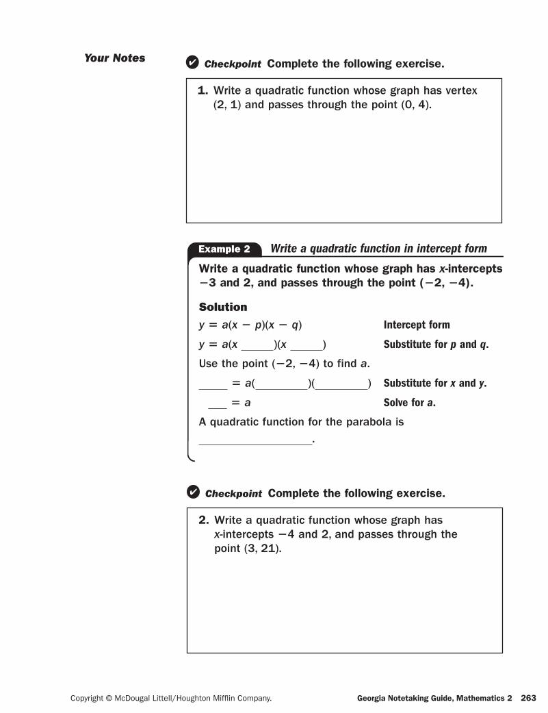
Write a quadratic function whose graph has vertex (22, 23) and passes through the point (0, 5).
Solutiony 5 a(x 2 h)2 1 k Vertex form
y 5 a(x )2 Substitute for h and k.
Use the point ( , ) to find a.
5 a( )2 Substitute for x and y.
5 a Solve for a.
A quadratic function for the parabola is .
Example 1 Write a quadratic function in vertex form
ga2nt-07.indd 157 4/16/07 9:04:08 AM
ga2_ntg_07.indd 262ga2_ntg_07.indd 262 4/19/07 3:47:15 PM4/19/07 3:47:15 PM
Copyright © McDougal Littell/Houghton Mifflin Company. Georgia Notetaking Guide, Mathematics 2 263
Your Notes
Write a quadratic function whose graph has x-intercepts23 and 2, and passes through the point (22, 24).
Solutiony 5 a(x 2 p)(x 2 q) Intercept form
y 5 a(x )(x ) Substitute for p and q.
Use the point (22, 24) to find a.
5 a( )( ) Substitute for x and y.
5 a Solve for a.
A quadratic function for the parabola is .
Example 2 Write a quadratic function in intercept form
1. Write a quadratic function whose graph has vertex (2, 1) and passes through the point (0, 4).
Checkpoint Complete the following exercise.
2. Write a quadratic function whose graph has x-intercepts 24 and 2, and passes through the point (3, 21).
Checkpoint Complete the following exercise.
ga2nt-07.indd 158 4/16/07 9:04:09 AM
ga2_ntg_07.indd 263ga2_ntg_07.indd 263 4/19/07 3:47:16 PM4/19/07 3:47:16 PM

264 Georgia Notetaking Guide, Mathematics 2 Copyright © McDougal Littell/Houghton Mifflin Company.
Your Notes
Write a quadratic function in standard form for the parabola that passes through the points (22, 26), (0, 6), and (2, 2).
Substitute the coordinates of each point into y 5 ax2 1 bx 1 c to obtain a system of three equations.
5 a( )2 1 b( ) 1 c Substitute for x and y.5 Equation 1
5 a( )2 1 b( ) 1 c Substitute for x and y.5 Equation 2
5 a( )2 1 b( ) 1 c Substitute for x and y.5 Equation 3
Rewrite the system as a system of two equations.
5 Substitute for c.5 Revised Equation 15 Substitute for c.5 Revised Equation 3
Solve the system consisting of revised Equations 1 and 3.
Revised Equation 1Revised Equation 3Add equations.
a 5 Solve for a.
So, 5 , which means b 5 .
A quadratic function for the parabola is .
Example 3 Write a quadratic function in standard form
Substitute 6 for cin Equation 1.
Substitute 6 for cin Equation 3.
3. Write a quadratic function in standard form for the parabola that passes through the points (21, 25), (2, 1), and (3, 21).
Checkpoint Complete the following exercise.
ga2nt-07.indd 159 4/16/07 9:04:10 AM
ga2_ntg_07.indd 264ga2_ntg_07.indd 264 4/19/07 3:47:18 PM4/19/07 3:47:18 PM

Copyright © McDougal Littell/Houghton Mifflin Company. Georgia Notetaking Guide, Mathematics 2 265
Your Notes
Baseball The table shows the height of a baseball that is hit, with x representing the time (in seconds) and y representing the baseball’s height (in feet). Use a graphing calculator to find the best-fitting quadratic model for the data.
Time, x 0 2 4 6 8
Height, y 3 28 40 37 26
Enter the data into two lists Make a scatter plot of of a graphing calculator. the data.
L1 L2 L30 32 284 406 378 26
L1(1)=0
Use the quadratic regression Check how well the model fits the data by graphing the model and the data in the same viewing window.
model feature to find the best-fitting quadratic model for the data.
QuadReg
y 5 ax2 1 bx 1 c
a 5
b 5
c 5
The best-fitting quadratic model is
.
Example 4 Best-fitting quadratic model for data
4. Use a graphing calculator to find the best-fitting model for the data in the table.
Time, x 0 2 4 6 8
Height, y 4 23 30 25 7
Checkpoint Complete the following exercise.
Homework
ga2nt-07.indd 160 4/16/07 9:04:11 AM
ga2_ntg_07.indd 265ga2_ntg_07.indd 265 4/19/07 3:47:19 PM4/19/07 3:47:19 PM

266 Georgia Notetaking Guide, Mathematics 2 Copyright © McDougal Littell/Houghton Mifflin Company.
Write a quadratic function in vertex form whose graph has the given vertex and passes through the given point.
1. vertex: (2, 0) 2. vertex: (1, 23) 3. vertex: (22, 2)
point: (3, 1) point: (0, 21) point: (0, 0)
Write a quadratic function in intercept form whose graph has the given x–intercepts and passes through the given point.
4. x-intercepts: 1, 4 5. x-intercepts: 23, 2 6. x-intercepts: 25, 0
point: (2, 26) point: (22, 24) point: (21, 8)
LESSON
7.2 Practice
Name ——————————————————————— Date ————————————
ga2_ntg_07.indd 266ga2_ntg_07.indd 266 4/19/07 3:47:21 PM4/19/07 3:47:21 PM

Copyright © McDougal Littell/Houghton Mifflin Company. Georgia Notetaking Guide, Mathematics 2 267
Name ——————————————————————— Date ————————————
LESSON
7.2 Practice continued
Write a quadratic function in standard form whose graph passes through the given points.
7. (22, 3), (0, 1), (2, 7) 8. (21, 2), (0, 22), (3, 22) 9. (0, 3), (1, 5), (2, 3)
In Exercises 10 and 11, use the following information.
Youth Football The table shows the number of participants y in a local youth football program from 2003 to 2008. Assume that t represents the number of years since 2003.
Year, t 0 1 2 3 4 5
Participants, y 24 28 33 41 54 74
10. Use a graphing calculator to fi nd the best-fi tting quadratic model for the data.
11. Using the model, how many participants are projected for 2011?
ga2_ntg_07.indd 267ga2_ntg_07.indd 267 4/19/07 3:47:21 PM4/19/07 3:47:21 PM

268 Georgia Notetaking Guide, Mathematics 2 Copyright © McDougal Littell/Houghton Mifflin Company.
7.3 Find Measures of Central Tendency and DispersionGoal p Describe data using statistical measures.Georgia
PerformanceStandard(s)
MM2D1b, MM2D1c
Your Notes
VOCABULARY
Statistics
Measure of central tendency
Mean
Median
Mode
Measure of dispersion
Range
Standard deviation
ga2nt-07.indd 161 4/16/07 9:04:12 AM
ga2_ntg_07.indd 268ga2_ntg_07.indd 268 4/19/07 3:47:22 PM4/19/07 3:47:22 PM

Copyright © McDougal Littell/Houghton Mifflin Company. Georgia Notetaking Guide, Mathematics 2 269
Your Notes
Find the mean, median, and mode of Quiz Scores
19, 15, 22,17, 21, 17,25, 18, 17
the data set.
Solution
To find the mean, divide the sum of the scores by the number of scores.
}x 5 5 5
To find the median, first order the quiz scores from least to greatest.
Because there is an odd number of scores, the median is the middle number, .
There is one mode, , because this number occurs most frequently.
Example 1 Find measures of central tendency
STANDARD DEVIATION OF A DATA SET
The standard deviation s (read as “sigma”) of x1, x2, . . . , xn is:
s 5 Î}}}}
}}}}n
Find the range and standard deviation for the quiz scores in Example 1.
Solution
To find the range, subtract the least data value from the greatest data value.
Range 5 2 5
To find the standard deviation, substitute the scores and the mean into the formula.
s 5 Î}}}}}
}}}}}
ø
Example 2 Find measures of dispersion
ga2nt-07.indd 162 4/16/07 9:04:13 AM
ga2_ntg_07.indd 269ga2_ntg_07.indd 269 4/19/07 3:47:23 PM4/19/07 3:47:23 PM

270 Georgia Notetaking Guide, Mathematics 2 Copyright © McDougal Littell/Houghton Mifflin Company.
Your Notes
The lists show the number of memberships sold each month for one year by two competing athletic clubs. Compare the mean and standard deviation for the numbers of memberships sold by the two athletic clubs.
Club A: 12, 9, 14, 6, 10, 11, 19, 6, 17, 11, 4, 13Club B: 17, 10, 22, 15, 14, 19, 4, 8, 12, 22, 20, 5
Solution
Club A: Mean: }x 5 5 5
Std. Dev.:
s 5 Î}}}}
}}}}
ø
Club B: Mean: }x 5 5 5
Std. Dev.:
s 5 Î}}}}
}}}}
ø
Athletic Club has a greater mean and a greater standard deviation than Athletic Club .
Example 3 Compare data sets
1. The data set below gives the recorded speeds (in mi/h) of 10 different cars on a local highway during a week day.
69, 62, 64, 67, 62, 64, 63, 65, 60, 64
Find the mean, median, and mode of the data set.
Checkpoint Complete the following exercise.
ga2nt-07.indd 163 4/16/07 9:04:13 AM
ga2_ntg_07.indd 270ga2_ntg_07.indd 270 4/19/07 3:47:24 PM4/19/07 3:47:24 PM

Copyright © McDougal Littell/Houghton Mifflin Company. Georgia Notetaking Guide, Mathematics 2 271
Your Notes
2. Find the range and standard deviation of the data set in Exercise 1.
3. Compare the means and standard deviations of Set A and Set B.
Set A 4 7 5 9 10
Set B 2 6 5 4 3
Checkpoint Complete the following exercises.
Homework
ga2nt-07.indd 164 4/16/07 9:04:14 AM
ga2_ntg_07.indd 271ga2_ntg_07.indd 271 4/19/07 3:47:25 PM4/19/07 3:47:25 PM

272 Georgia Notetaking Guide, Mathematics 2 Copyright © McDougal Littell/Houghton Mifflin Company.
Find the mean, median, and mode of the data set.
1. 1, 6, 3, 9, 6, 8, 4, 4, 4 2. 1, 5, 6, 2, 6, 1, 7, 6, 2
3. 17, 13, 12, 12, 13, 16, 12, 13, 14, 10 4. 12, 14, 11, 15, 14, 18, 9, 11, 13, 10
Find the range and standard deviation of the data set.
5. 12, 8, 17, 15, 12, 14 6. 17, 14, 24, 21, 30, 20
7. 22, 24, 31, 34, 23, 27, 21 8. 31, 46, 39, 43, 32, 35, 40
In Exercises 9 and 10, fi nd the mean, median, mode, range, and standard deviation of the data set.
9. Quiz Scores The data set below gives the quiz scores for a student on quizzes consisting of 10 points each.
7, 9, 7, 10, 8, 7, 9
10. Travel Distance The data set below gives the distances (in miles) that several people travel to and from work each day.
12, 15, 11, 8, 11, 13, 10, 16
LESSON
7.3 Practice
Name ——————————————————————— Date ————————————
ga2_ntg_07.indd 272ga2_ntg_07.indd 272 4/19/07 3:47:26 PM4/19/07 3:47:26 PM

Copyright © McDougal Littell/Houghton Mifflin Company. Georgia Notetaking Guide, Mathematics 2 273
Name ——————————————————————— Date ————————————
LESSON
7.3 Practice continued
In Exercises 11 and 12, fi nd the mean, median, mode, range, and standard deviation of the data set.
11. Oil Change The data set below gives the waiting times (in minutes) for several people having the oil changed in their cars at an auto mechanics shop.
22, 18, 25, 21, 28, 26, 20, 28, 20
12. Hockey The data set below gives the numbers of goals for the 10 players who scored the most goals during the 2003–2004 National Hockey League regular season.
41, 41, 41, 38, 38, 36, 35, 35, 34, 33
13. Telephone Calls The data sets below give the lengths (in minutes) of long distance telephone calls made from a household during two months. Compare the mean and standard deviation for the calls made during the two months.
Month A: 11, 15, 10, 37, 17, 14, 9, 15
Month B: 13, 9, 16, 8, 17, 20, 8, 13
ga2_ntg_07.indd 273ga2_ntg_07.indd 273 4/19/07 3:47:26 PM4/19/07 3:47:26 PM

274 Georgia Notetaking Guide, Mathematics 2 Copyright © McDougal Littell/Houghton Mifflin Company.
7.4 Use Normal DistributionsGoal p Study normal distributions.Georgia
PerformanceStandard(s)
MM2D1d
Your Notes
VOCABULARY
Normal distribution
Normal curve
Standard normal distribution
z-score
AREAS UNDER A NORMAL CURVE
A normal distribution with mean }x and standard deviation s has these properties:
• The total area under the related normal curve is .
• About % of the area lies within 1 standard deviation of the mean.
• About % of the area lies within 2 standard deviations of the mean.
• About % of the area lies within 3 standard deviations of the mean.
x2
3s
x2
2s
x2
s x
x1
s
x1
2s
x1
3s
68%
95%
99.7%
x2
3s
x2
2s
x2
s x
x1
s
x1
2s
x1
3s
2.35% 2.35%
0.15% 0.15%
13.5% 13.5%
34% 34%
ga2nt-07.indd 165 4/16/07 9:04:15 AM
ga2_ntg_07.indd 274ga2_ntg_07.indd 274 4/19/07 3:47:26 PM4/19/07 3:47:26 PM

Copyright © McDougal Littell/Houghton Mifflin Company. Georgia Notetaking Guide, Mathematics 2 275
Your Notes
A normal distribution has mean
x2
3s
x2
2s
x2
s x
x1
s
x1
2s
x1
3s
}x and standard deviation s. For a randomly selected x-value from the distribution, find P(}x 2 s ≤ x ≤ }x 1 2s).
SolutionThe probability that a randomly selected x-value lies between and is the shaded area under the normal curve. Therefore:
P(}x 2 s ≤ x ≤ }x 1 2s) 5 1 1
5
Example 1 Find a normal probability
1. A normal distribution has mean }x and standard deviation s. For a randomly selected x-value from the distribution, find P(x ≤ }x 2 s).
Checkpoint Complete the following exercise.
Math Scores The math scores of an
169 278 387 496 605 714 823
exam for the state of Georgia are normally distributed with a mean of 496 and a standard deviation of 109. About what percent of the test-takers received scores between 387 and 605?
Solution
The scores of 387 and 605 repressent standard deviation on either side of the mean. So, the percent of test-takers with scores between 387 and 605 is
% 1 % 5 %.
Example 2 Interpret normally distributed data
ga2nt-07.indd 166 4/16/07 9:04:15 AM
ga2_ntg_07.indd 275ga2_ntg_07.indd 275 4/19/07 3:47:28 PM4/19/07 3:47:28 PM

276 Georgia Notetaking Guide, Mathematics 2 Copyright © McDougal Littell/Houghton Mifflin Company.
Your Notes
2. In Example 2, what percent of the test-takers received scores between 496 and 714?
3. In Example 3, find the probability that a randomly selected test-taker received a math score of at most 620.
Checkpoint Complete the following exercises.
Homework
In Example 2, find the probability that a randomly selected test-taker received a math score of at most 630.
SolutionStep 1 Find the z-score corresponding to an x-value
of 630.
z 5x 2 }x}
s5 ø
Step 2 Use the standard normal table to findP(x ≤ 630) ø P(z ≤ ).
z .0 .1 .2
23 .0013 .0010 .0007
22 .0228 .0179 .0139
21 .1587 .1357 .1151
20 .5000 .4602 .4207
0 .5000 .5398 .5793
1 .8413 .8643 .8849
The table shows that P(z ≤ ) 5 .
So, the probability that a randomly selected test-taker received a math score of at most 630 is about .
Example 3 Use a z-score and the standard normal table
ga2nt-07.indd 167 4/16/07 9:04:16 AM
ga2_ntg_07.indd 276ga2_ntg_07.indd 276 4/19/07 3:47:29 PM4/19/07 3:47:29 PM
Copyright © McDougal Littell/Houghton Mifflin Company. Georgia Notetaking Guide, Mathematics 2 277
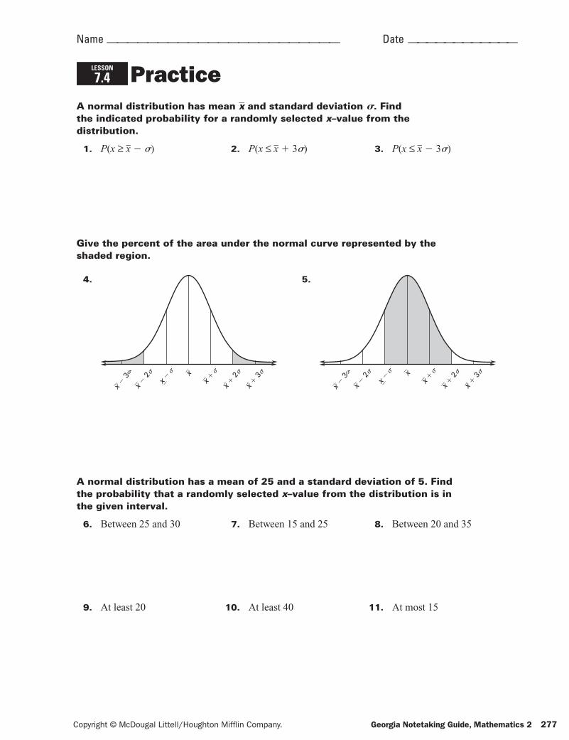
Name ——————————————————————— Date ————————————
LESSON
7.4 PracticeA normal distribution has mean } x and standard deviation s. Find the indicated probability for a randomly selected x–value from the distribution.
1. P(x ≥ } x 2 s) 2. P(x ≤ } x 1 3s) 3. P(x ≤ } x 2 3s)
Give the percent of the area under the normal curve represented by the shaded region.
4.
s
x 2
3
s
x 2
2
s
x 2
x s
x 1
s
x 1
2
s
x 1
3
5.
s
x 2
3
s
x 2
2s
x 2
x s
x 1
s
x 1
2
s
x 1
3A normal distribution has a mean of 25 and a standard deviation of 5. Find the probability that a randomly selected x–value from the distribution is in the given interval.
6. Between 25 and 30 7. Between 15 and 25 8. Between 20 and 35
9. At least 20 10. At least 40 11. At most 15
ga2_ntg_07.indd 277ga2_ntg_07.indd 277 4/19/07 3:47:30 PM4/19/07 3:47:30 PM

278 Georgia Notetaking Guide, Mathematics 2 Copyright © McDougal Littell/Houghton Mifflin Company.
A normal distribution has a mean of 75 and a standard deviation of 10. Use the standard normal table of your textbook to fi nd the indicated probability for a randomly selected x–value from the distribution.
12. P(x ≤ 75) 13. P(x ≤ 85) 14. P(x ≤ 55)
15. P(x ≤ 87) 16. P(x ≤ 69) 17. P(x ≤ 45)
In Exercises 18 and 19, use the following information.
Breakfast A restaurant is busiest on Sunday from 6:00 A.M. to 9:00 A.M. During these hours, the waiting time for customers in groups of 5 or less to be seated is normally distributed with a mean of 20 minutes and a standard deviation of 4 minutes.
18. What is the probability that customers in groups of 5 or less will wait 8 minutes or less to be seated during the busy Sunday morning hours?
19. What is the probability that customers in groups of 5 or less will wait 24 minutes or more to be seated during the busy Sunday morning hours?
In Exercises 20 and 21, use the following information.
Light Bulbs A company produces light bulbs having a life expectancy that is normally distributed with a mean of 1800 hours and a standard deviation of 65 hours.
20. Find the z-score for a life expectancy of 2000 hours.
21. What is the probability that a randomly selected light bulb will last at most 2000 hours?
LESSON
7.4 Practice continued
Name ——————————————————————— Date ————————————
ga2_ntg_07.indd 278ga2_ntg_07.indd 278 4/19/07 3:47:31 PM4/19/07 3:47:31 PM

Copyright © McDougal Littell/Houghton Mifflin Company. Georgia Notetaking Guide, Mathematics 2 279
7.5 Select and Draw Conclusions from SamplesGoal p Study different sampling methods for
collecting data.
GeorgiaPerformanceStandard(s)
MM2D1a
Your NotesVOCABULARY
Population
Sample
Unbiased sample
Biased sample
Population mean
Margin of error
MARGIN OF ERROR FORMULA
When a random sample of size n is taken from a large population, the margin of error is approximated by:
Margin of error 5 6
This means that if the percent of the sample responding a certain way is p (expressed as a decimal), then the percent of the population that would respond the same
way is likely to be between p 2 and p 1 .
ga2nt-07.indd 168 4/16/07 9:04:17 AM
ga2_ntg_07.indd 279ga2_ntg_07.indd 279 4/19/07 3:47:31 PM4/19/07 3:47:31 PM

280 Georgia Notetaking Guide, Mathematics 2 Copyright © McDougal Littell/Houghton Mifflin Company.
Your Notes
Assemblies A student wants to survey everyone at his school about the quality of the school's assemblies. Identify the type of sample described as a self-selectedsample, a systematic sample, a convenience sample, or a random sample.
a. The student surveys every 8th student that enters the assembly.
b. From a random name lottery, the student chooses 125 students and teachers to survey
Solutiona. The student uses a rule to select students, so the
sample is a sample.
b. The student chooses from a random name lottery, so the sample is a sample.
Example 1 Classify samples
1. A local mayor wants to survey local area registered voters. She mails surveys to the individuals that are members of her political party and uses only the surveys that are returned.
Checkpoint Identify the type of sample described.
Tell whether each sample in Example 1 is biased or unbiased. Explain your reasoning.
Solution
a. The sample is because the student surveys the students, but not the teachers.
b. The sample is because both students and teachers are surveyed.
Example 2 Identify biased solutions
ga2nt-07.indd 169 4/16/07 9:04:18 AM
ga2_ntg_07.indd 280ga2_ntg_07.indd 280 4/19/07 3:47:32 PM4/19/07 3:47:32 PM

Copyright © McDougal Littell/Houghton Mifflin Company. Georgia Notetaking Guide, Mathematics 2 281
Your Notes
Newspaper Survey In a survey of 325 students and teachers, 30% said they read the school's newspaper every weekday. (a) What is the margin of error for the survey? (b) Give an interval that is likely to contain the exact percent of all students and teachers who read the school's newspaper every weekday.
Solution
a. Margin of error 5 61
}Ï
}
n5 6
1ø
The margin of error for the survey is about %.
b. To find the interval, add and subtract %.
30% 2 % 5 %
30% 1 % 5 %
It is likely that the exact percent of all students and teachers who read the school's newspaper every weekday is between % and %.
Example 3 Find a margin of error
2. Tell whether the sample in Exercise 1 is biased or unbiased. Explain your reasoning.
3. In Example 3, suppose the sample size is 400 students and teachers. What is the margin of error for the survey?
Checkpoint Complete the following exercises.
Homework
ga2nt-07.indd 170 4/16/07 9:04:18 AM
ga2_ntg_07.indd 281ga2_ntg_07.indd 281 4/19/07 3:47:33 PM4/19/07 3:47:33 PM

282 Georgia Notetaking Guide, Mathematics 2 Copyright © McDougal Littell/Houghton Mifflin Company.
Identify the type of sample described. Then tell if the sample is biased. Explain your reasoning.
1. A gym is conducting a survey to fi nd out how often members attend the gym each week. A gym employee asks every other person attending the gym on a particular weekend.
2. A clothing store wants to know the favorite seasons of its customers. Surveys are placed on a table for customers to fi ll out as they enter the store.
3. A company wants to know how often its employees use the company’s cafeteria for lunch. The company asks employees that have just fi nished eating lunch in the cafeteria on Friday.
Find the margin of error for a survey that has the given sample size. Round your answer to the nearest tenth of a percent.
4. 375 5. 7000 6. 120
7. 3200 8. 385 9. 4500
10. 705 11. 85 12. 5005
LESSON
7.5 Practice
Name ——————————————————————— Date ————————————
ga2_ntg_07.indd 282ga2_ntg_07.indd 282 4/19/07 3:47:36 PM4/19/07 3:47:36 PM
Copyright © McDougal Littell/Houghton Mifflin Company. Georgia Notetaking Guide, Mathematics 2 283
Name ——————————————————————— Date ————————————
LESSON
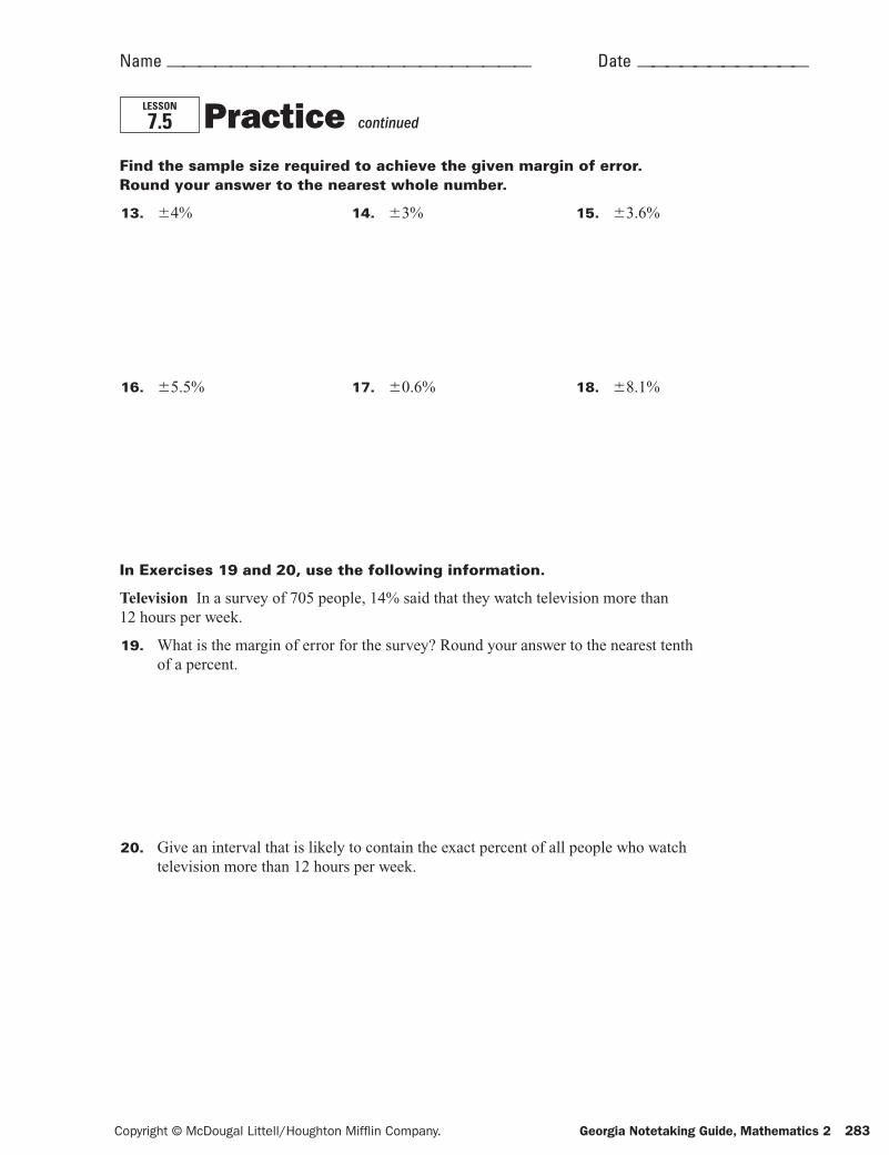
7.5 Practice continued
Find the sample size required to achieve the given margin of error. Round your answer to the nearest whole number.
13. 64% 14. 63% 15. 63.6%
16. 65.5% 17. 60.6% 18. 68.1%
In Exercises 19 and 20, use the following information.
Television In a survey of 705 people, 14% said that they watch television more than 12 hours per week.
19. What is the margin of error for the survey? Round your answer to the nearest tenth of a percent.
20. Give an interval that is likely to contain the exact percent of all people who watch television more than 12 hours per week.
ga2_ntg_07.indd 283ga2_ntg_07.indd 283 4/19/07 3:47:36 PM4/19/07 3:47:36 PM

284 Georgia Notetaking Guide, Mathematics 2 Copyright © McDougal Littell/Houghton Mifflin Company.
7.6 Sample Data and PopulationsGeorgiaPerformanceStandard(s)
MM2D1a, MM2D1d
Your Notes
Goal p Collect sample data from populations.
A gym has 467 female members and 732 male members. The marketing director of the gym wants to form a random sample of 30 female members and a separate random sample of 60 male members to answer some survey questions. Each female member has a membership number from 1 to 467 and each male member has a membership number from 1001 to 1732. Use a graphing calculator to select the members who will participate in each random sample.
Random sample of female members:
Using the random integer feature of a graphing calculator to generate random integers between and produces the following sample answer.
The random sample of female members have membership numbers
.
Random sample of male members:
Using the random integer feature of a graphing calculator to generate random integers between and produces the following sample answer.
The random sample of male members have membership numbers
.
Example 1 Collect data by randomly sampling
1. In Example 1, suppose there are 245 female members and 532 male members. The marketing director wants to form a random sample of 12 female members and a separate random sample of 15 male members. Use a graphing calculator to select the members who will participate in each random sample.
Checkpoint Complete the following exercise.
ga2nt-07.indd 171 4/16/07 9:04:19 AM
ga2_ntg_07.indd 284ga2_ntg_07.indd 284 4/19/07 3:47:36 PM4/19/07 3:47:36 PM

Copyright © McDougal Littell/Houghton Mifflin Company. Georgia Notetaking Guide, Mathematics 2 285
Your Notes
2. In Example 2, suppose the population mean is 14.5 and the population standard deviation is 10.4. Compare the means and standard deviations of the random samples to the population parameters.
Checkpoint Complete the following exercise.
Homework
A company wants to know how many minutes it takes their employees to drive to work each day. Gillian and Ted, two employees, collect separate random samples. Their results are displayed below. The population mean is 18.4 and the population standard deviation is about 15.6. Compare the means and standard deviations of the random samples to the population parameters.
Gillian10, 8, 20, 42, 5, 32, 8, 9, 17, 27
Ted23, 18, 6, 47, 23, 31, 10, 13, 7, 3, 14, 55, 25, 19, 23
Solution
Gillian: }x 5 5 5
Ted: }x 5 5 5
Gillian: s 5 Î}}}}}
ø
Ted: s 5 Î}}}}}
ø
The mean of Gillian's sample is the population mean, while the mean of Ted's sample is the population mean. The standard deviations of both samples are the population standard deviation.
Example 2 Compare statistics and parameters
ga2nt-07.indd 172 4/16/07 9:04:20 AM
ga2_ntg_07.indd 285ga2_ntg_07.indd 285 4/19/07 3:47:37 PM4/19/07 3:47:37 PM

286 Georgia Notetaking Guide, Mathematics 2 Copyright © McDougal Littell/Houghton Mifflin Company.
In Exercises 1–6, use a graphing calculator to generate fi ve random integers in the given range.
1. 1 to 100 2. 200 to 400 3. 101 to 450
4. 25 to 1000 5. 60 to 70 6. 1001 to 1765
For a large population, the mean is 11.2 and the standard deviation is about 8.4. Compare the mean and standard deviation of the random sample to the population parameters.
7. Random Sample A14, 28, 19, 11, 14, 25, 27, 8, 22, 15
8. Random Sample B15, 7, 3, 11, 20, 5, 20, 1, 18, 9
9. Random Sample C
1, 28, 26, 8, 22, 8, 4, 22, 7, 18, 25, 29
10. Movies Two students want to know the number of DVDs owned by each student in their school. Jake and Juan collect separate random samples. The population mean is 14.3 and the population standard deviation is about 6.7. Compare the means and standard deviations of the random samples to the population parameters.
Jake15, 3, 13, 20, 11, 25, 22, 1, 12, 12, 7, 6, 8, 24, 14, 10, 22, 29, 22, 4, 12, 18, 18, 11, 7
Juan
9, 27, 6, 16, 10, 22, 29, 28, 20, 21, 1, 4, 24, 12, 16, 15, 28, 12, 6, 13, 30, 8
LESSON
7.6 Practice
Name ——————————————————————— Date ————————————
ga2_ntg_07.indd 286ga2_ntg_07.indd 286 4/19/07 3:47:39 PM4/19/07 3:47:39 PM

Copyright © McDougal Littell/Houghton Mifflin Company. Georgia Notetaking Guide, Mathematics 2 287
7.7 Choose the Best Model for Two-Variable DataGoal p Choose the best model to represent a set of data.Georgia
PerformanceStandard(s)
MM2D2a, MM2D2c
Your Notes
Teachers' Salaries The table shows the teacher's salary y (in dollars) for a certain school district, where x is the number of years of teaching experience. Use a graphing calculator to find a model for the data.
x 1 2 3 4
y 30,624 32,436 34,167 35,989
x 5 6 7
y 37,684 39,311 41,098
1. Make a scatter plot. The points lie approximately on a .This suggests a model.
2. Use the regression feature to find an equation of the model.
3. Graph the model along with the data to verify that the model fits the data well.
A model for the data is y 5 .
Example 1 Use a linear model
1. Use a graphing calculator to find
x
y
10
1
a model for the data. Then graph the model and the data in the same coordinate plane.
x 0 1 2 3
y 2 9 19 29
x 4 5 6 7
y 40 51 61 73
Checkpoint Complete the following exercise.
ga2nt-07.indd 173 4/16/07 9:04:20 AM
ga2_ntg_07.indd 287ga2_ntg_07.indd 287 4/19/07 3:47:39 PM4/19/07 3:47:39 PM

288 Georgia Notetaking Guide, Mathematics 2 Copyright © McDougal Littell/Houghton Mifflin Company.
Your Notes
Homework
Roller Coaster Riders A manager at a local amusement park kept a record of the number of people who ride the most popular roller coaster at the park. The table shows the number of people y who rode the roller coaster x hours after the park had opened. Use a graphing calculator to find a model for the data.
x 0 2 4 6 8 10 12
y 85 163 282 341 398 381 304
Solution1. Make a scatter plot. The points
form an .This suggests a model.
2. Use the regression feature to find an equation of the model.
3. Graph the model along with the data to verify that the model fits the data well.
A model for the data is y 5 .
Example 2 Use a quadratic model
2. Use a graphing calculator to find a model for the data. Then graph the model and the data in the same coordinate plane.
x 0 2 4 6 8 10 12
y 100 178 273 314 349 324 289
x
y
40
2
Checkpoint Complete the following exercise.
ga2nt-07.indd 174 4/16/07 9:04:23 AM
ga2_ntg_07.indd 288ga2_ntg_07.indd 288 4/19/07 3:47:41 PM4/19/07 3:47:41 PM

Copyright © McDougal Littell/Houghton Mifflin Company. Georgia Notetaking Guide, Mathematics 2 289
Name ——————————————————————— Date ————————————
LESSON
7.7 PracticeUse a graphing calculator to fi nd the equation that best models the data.
1. x 1 2 3 4 5 6 7
y 2 3 5 6 8 9 11
2. x 2 5 7 10 12 14 18
y 21 29 35 40 37 32 23
3. x 1 2 3 4 5 6 7
y 5 11 20 31 42 56 65
4. x 5 10 15 20 25 30 35
y 22 31 44 65 86 104 123
5. x 3 6 10 15 18 22 27
y 2 3 4 7 9 13 21
6. Drive-Thru Banking A bank records the length of time y (in minutes) that a customer has to wait each hour before getting service at the drive-thru window. The bank provides drive-thru service from 9:00 A.M. to 4:30 P.M. (x 5 1 represents 9:00 A.M.) Use the regression feature of a graphing calculator to fi nd a model for the data. If the bank extended its drive-thru hours, how long would a customer have to wait at 5:00 P.M.? Round your answer to the nearest whole minute.
x 1 2 3 4 5 6 7 8
y 3 5 6 8 7 8 8 9
ga2_ntg_07.indd 289ga2_ntg_07.indd 289 4/19/07 3:47:42 PM4/19/07 3:47:42 PM

290 Georgia Notetaking Guide, Mathematics 2 Copyright © McDougal Littell/Houghton Mifflin Company.
Words to ReviewGive an example of the vocabulary word.
Scatter plot
Negative correlation
Best-fitting line
Positive correlation
Correlation coefficient
Linear regression
ga2nt-07.indd 175 4/16/07 9:04:24 AM
ga2_ntg_07.indd 290ga2_ntg_07.indd 290 4/19/07 3:47:43 PM4/19/07 3:47:43 PM

Copyright © McDougal Littell/Houghton Mifflin Company. Georgia Notetaking Guide, Mathematics 2 291
Median-median line
Inference
Best-fitting quadratic model
Statistics
Measure of dispersion
Range:
Standard deviation:
Algebraic model
Quadratic regression
Curve fitting
Measure of central tendency
Mean:
Median:
Mode:
Normal distribution
ga2nt-07.indd 176 4/16/07 9:04:25 AM
ga2_ntg_07.indd 291ga2_ntg_07.indd 291 4/19/07 3:47:44 PM4/19/07 3:47:44 PM

292 Georgia Notetaking Guide, Mathematics 2 Copyright © McDougal Littell/Houghton Mifflin Company.
Normal curve
z-score
Sample
Biased sample
Margin of error
Standard normal distribution
Population
Unbiased sample
Population mean
ga2nt-07.indd 177 4/16/07 9:04:25 AM
ga2_ntg_07.indd 292ga2_ntg_07.indd 292 4/19/07 3:47:46 PM4/19/07 3:47:46 PM
Related Documents