Draft version November 16, 2005 arXiv:astro-ph/0511414 v1 ...hubblesite.org/pubinfo/pdf/2006/04/pdf2.pdf · Draft version November 16, 2005 ... is the deepest optical image of a slice

arX

iv:a

stro

-ph/

0511

414

v1

14 N

ov 2

005

Draft version November 16, 2005Preprint typeset using LATEX style emulateapj v. 04/21/05

CLUES TO AGN GROWTH FROM OPTICALLY VARIABLE OBJECTSIN THE HUBBLE ULTRA DEEP FIELD

S. H. Cohen, R. E. Ryan Jr., A. N. Straughn, N. P. Hathi, R. A. WindhorstDepartment of Physics and Astronomy, Arizona State University, Tempe, AZ 85287-1504

and

A. M. Koekemoer, N. Pirzkal, C. Xu, B. Mobasher, S. Malhotra, L.-G. Strolger, J. E. RhoadsSpace Telescope Science Institute, Baltimore, MD 21218

Draft version November 16, 2005

ABSTRACT

We present a photometric search for objects with point-source components that are optically variableon timescales of weeks–months in the Hubble Ultra Deep Field (HUDF) to i′AB = 28.0 mag. Thedata are split into four sub-stacks of approximately equal exposure times. Objects exhibiting thesignature of optical variability are selected by studying the photometric error distribution betweenthe four different epochs, and selecting 622 candidates as 3.0σ outliers from the original catalog of4644 objects. Of these, 45 are visually confirmed as free of contamination from close neighbors orvarious types of image defects. Four lie within the positional error boxes of Chandra X-ray sources,and two of these are spectroscopically confirmed AGN. The photometric redshift distribution of theselected variable sample is compared to that of field galaxies, and we find that a constant fraction of∼1% of all field objects show variability over the range of 0.1.z .4.5. Combined with other recentHUDF results, as well as those of recent state-of-the-art numerical simulations, we discuss a potentiallink between the hierarchical merging of galaxies and the growth of AGN.

Subject headings: Galaxies: active — galaxies: formation — Active Galactic Nuclei — SupermassiveBlack Holes

1. INTRODUCTION

The Hubble Ultra Deep Field (HUDF; Beckwith et al.2005) is the deepest optical image of a slice of the Uni-verse ever observed. As such, it allows for a varietyof different investigations into astrophysical objects andprocesses. The HUDF observations consist of 400 orbitswith the Hubble Space Telescope (HST) over a period offour months in four optical bands (BV i′z′) with the Ad-vanced Camera for Surveys (ACS), and are supplementedin the JH bands with an HST Legacy Program using theNear-Infrared Camera and Multi-Object Spectrograph(NICMOS; Bouwens et al. 2004; Thompson et al. 2005).Given the unprecedented quality of these data, the listof supporting data from both space and the ground isconstantly growing.

Since the ACS data was observed over a period of fourmonths, it provides a unique opportunity to search forvariability in all types of objects to very faint flux levels(perhaps even for AB & 30 mag), such as faint stars, dis-tant supernovae (SNe), and weak active galactic nuclei(AGN). In this paper, we search for weak AGN vari-ability in the i′-band (F775W), because, in this filter,the HUDF images are deepest, and have the best tem-poral spacing over the four months for the variabilitysearch. It should be noted that at higher redshifts, theACS filters sample further into the rest-frame ultraviolet.This is advantageous, because AGNs are known to showmore variability in the UV (e.g., Paltani & Courvoisier1994). In the original Hubble Deep Field North (HDF–N) and the Groth Strip Survey, Sarajedini et al. (2003)and Sarajedini (2003) performed a similar search toAB=27.0 mag over longer time baselines (5–7 years).

Electronic address: [email protected]

They searched for variability in the nuclei of the galaxiesusing small apertures, which is a different approach thanin the present search.

From the WMAP polarization results (Kogut et al.2003), population III stars likely existed at z≃20. Thesemassive stars (& 250 M⊙) are expected to produce alarge population of massive black holes (Mbh &150 M⊙,Madau & Rees (2001)). Since there is now good dy-namical evidence for the existence of supermassive(Mbh ≃ 106−109 M⊙) black holes (SMBH) in the cen-ters of galaxies at z ≃ 0 (Kormendy & Richstone1995; Magorrian, Tremaine, & Richstone 1998;Kormendy & Gebhardt 2001), it is important tounderstand if there is any relationship between theformation of the SMBHs observed at z ≃ 0 and thelower mass BHs at z≃20. A comprehensive reviewof SMBHs is given by Ferrarese & Ford (2004). Animportant question to address is how these SMBHs,as seen nearby, have grown over the course of cosmictime. One suggestion is that they “grow” throughthe mergers of galaxies that themselves contain lessmassive BHs, so the byproduct is a larger single galaxywith–eventually–a more massive BH in its center. Thegrowth of the BH may then be observed via its AGNactivity. If this scenario is true, then perhaps thereexists an observable link between galaxy mergers andincreased AGN activity (Silk & Rees 1998). Therefore,studying this possible link as a function of redshift couldgive insight into the growth of SMBHs and its potentialrelation to the process of galaxy assembly.

In §2, we present the HUDF observations and sum-marize the essential elements of its data reduction, andin §3 we present the variable candidate selection. In §4we present the photometric redshift distribution of the

2 Cohen et al.

TABLE 1Observations

Epoch Start End Exp. Timea # of RJDb Days SinceNo. Date Date (Seconds) Exp. (Days) Epoch 1

1 2003-09-24 2003-10-10 92340 76 52914.2 · · ·2 2003-10-10 2003-10-29 92340 76 52926.7 12.53 2003-12-04 2003-12-18 89940 76 52985.9 71.74 2003-12-22 2004-01-14 72490 60 53005.7 91.5

aThere are two exposures per HST orbitbRJD=median Revised Julian Date−2.4×106 days

variable objects together with that of the HUDF fieldgalaxies, in §5 we present the results, and in §6 we dis-cuss our results in terms of galaxy assembly and AGNgrowth.

2. OBSERVATIONS

All data used here are from the Hubble Ultra DeepField (HUDF; Beckwith et al. 2005). The individualcosmic-ray (CR) clipped images and weight maps wereused with multidrizzle (Koekemoer et al. 2002) to createeight sub-stacks of approximately equal exposure times.These used the same cosmic-ray maps and weight mapsemployed to create the full-depth HUDF mosaics. AllHUDF images were drizzled onto the same output pixelscale (0.′′030 per pixel) and WCS frame as the originalHUDF. Given the time-spacing of the exposures andthe desire to extend the study to the faintest possibleflux-levels, the images and weight maps were combinedin groups of two to create four epochs of observationfor the variability study on 0.4–3.5 months timescales.Exposure–time weighted averages were created for allimages, and simple addition was used to combine theweight maps (Beckwith et al. 2005). The exposure timesand median observation dates are listed in Table 1. Thefour epochs chosen here have exposure times as close toeach other as possible, so that the flux error distribu-tions will be as much as possible symmetric, and there-fore more easily modeled. As seen in Table 1, this is doneat the expense of not having the endpoints of the fourepochs well-spaced in time. In order to be optimizedfor variability studies, future observations of this kindshould take into account the need for both equal depthexposures and well separated observation dates, althoughthis would further complicate the already difficult taskof scheduling observations such as the HUDF. All magni-tudes are on the AB-system using the zero-points givenin the HUDF public data release (Beckwith et al. 2005).

2.1. Catalog Generation and Photometry

Variability was searched for by comparing the photo-metric catalogs from the various epochs to each other.Catalogs were generated using SExtractor Version 2.2.2(Bertin & Arnouts 1996) with a 1.0σ detection thresh-old, and requiring a minimum of 15 connected pixels(i.e. aproximately the PSF area) at this limit abovesky. Since we are searching for any signs of variabil-ity, we chose to use a liberal amount of de-blending(DEBLEND MINCONT = 5×10−6). This allows forpieces of merging galaxies to be measured separately toenhance the chances of finding variable events in point-source components. SExtractor was run in dual imagemode using the full-depth HUDF as the detection image,

and utilizing the corresponding weight-maps to minimizethe number of false detections due to edges and otherimage defects that are reflected in these weight-maps.This results in catalogs with 27819 measured objects,which still contains many over-deblended objects or edge-effects. Since the HUDF was observed at four differentposition angles (Beckwith et al. 2005), only the 15205 ob-jects observed in all four epochs were considered. The re-sult is a catalog of 12514 objects, which is 90% completeto i′ . 30.5 mag. Since we can only measure variabil-ity from the individual epoch images that are one-fourththe full HUDF in length, the variable candidate sampleis restricted to the 4644 objects with i′<28.0 mag.

The HUDF is the deepest optical image ever observed,and will possibly remain the deepest until the JamesWebb Space Telescope (JWST) is launched in 2011. Toexplore the limits of the HUDF depth, a few words aboutthe point spread function (PSF) of the ACS images areneeded. A comprehensive study of HST/ACS PSF-issuescan be found in Heymans et al. (2004), so here we onlyhighlight the aspects relevant to our study. First, theACS camera is not located on the optical axis of HST,and therefore the HUDF field is rectified by applying ge-ometric distortion correction polynomials. Secondly, theACS/WFC PSF is known to vary with location on theCCD detectors, and with the time of observation dueto “breathing” of the HST Optical Telescope Assembly(OTA). Since the HUDF was observed at four differentroll angles over four months, these PSF effects can easilybe seen by inspecting the locations of bright objects inan image created by dividing two images taken at dif-ferent roll angles. Owing to these PSF issues and thesignificantly complex ACS image registration, this “ratio-image” will easily show the cores of all bright objects withsignificant positive or negative flux excursions, regardlessof whether or not they are truly variable. For this rea-son, we cannot use small PSF-sized apertures to searchfor nuclear variability, as was done by Sarajedini et al.(2003). Sarajedini et al. (2003) could use the small–aperture method, because for the much larger WFPC2pixel-size and the on-axis location of the WFPC2 cam-era, the geometrical distortion correction and registra-tion effects are much smaller. Instead, we chose to usetotal magnitudes of the highly deblended objects. Eventhough our total flux apertures may encompass the wholegalaxy, the variability necessarily must come from a smallregion (less than the 0.′′084 PSF), due to the finite light-travel time across the region of variability.

3. CANDIDATE SELECTION

The catalogs of the four epochs were all compared toeach other resulting in six sets of diagrams similar to theone shown in Fig. 1. These figures show the change inmeasured magnitudes in the SExtractor matched aper-tures as a function of full-depth HUDF flux. In order todetermine which objects were true outliers (i.e., variablecandidates), the expected error distribution for each setwas computed as follows. For each measurement in agiven epoch, we compute the total flux error for that ith

flux measurement:

σtoti =

√

σ2i A(Fi) + Fi/G

F 2i

(1)

Variability in the HUDF 3

Fig. 1.— Magnitude difference between two HUDF epochs ofall objects versus their total i′-band flux in AB-mag from matchedtotal apertures. The ±1σ,±3σ,±5σ lines are shown. The blackcircles show the 222 variable candidates chosen to be |∆mag| &3σoutliers between any one of these these two epochs and 20 . i′ .28.0 mag. Blue points show the |∆mag| ≤ ±1σ points used tonormalize the error distribution, so that 1.0σ reflects as much aspossible the true Gaussian 1-σ line. Large red points show the“best” 45 candidates that were chosen from all six possible epochcombinations, many of which were seen at & 3.0σ in 2 or moreepoch combinations.

where σi is the RMS per pixel in the sky background,A(Fi) is the number of pixels belonging to object i of agiven flux (described in detail below), Fi is its measuredflux in e− per second and G is the gain in units of seconds.This quantity is computed for each epoch, and for eachof the epoch-pairs they are combined in quadrature:

∆mag = ±

√

(1.0857N)2 ×(

(σtoti )2 + (σtot

j )2)

(2)

where N is the number of σ for which the error-model iscomputed, and i, j denote the measurements at a givenflux-level in each of the two epochs under consideration.Since each object at a given flux level can have a differ-ent area A (i.e., number of pixels), we need to assume ageneral relation between flux and area in order to opti-mally model the true error distribution using the aboveequations. This relation was determined iteratively foreach pair of observations, such that 68.3% of the pointslie within the boundaries of the upper and lower 1.0σlines. We started this process by fitting the relation be-tween the SExtractor magnitude and ISOAREA IMAGEparameters as a first guess. It is then assumed that flux isproportional to area, and we solve iteratively for the pro-portionality constant to get ±1.0σ lines that maximallyrepresent a Gaussian error distribution (Fig. 1). In orderto demostrate the Gaussian nature of this error distri-bution at all flux levels, the ∆mag data are divided bythe 1.0–σ model line, and histograms were computed forthe resulting ∆mag data at various flux-levels (Fig. 2).These histograms are remarkably well fit by Gaussiansof σ ≃ 1. The HUDF noise distribution is not perfectlyGaussian, but with 288 independent exposures in the i′-band, the error distribution is as close to Gaussian asseen in any astronomical CCD application.

Once this 1σ line is determined, we set N = 3.0 inEqn. 2, and find all the objects that are at least 3.0σoutliers. In Fig. 1, we show the ±1σ, ±3σ, and ±5σ

Fig. 2.— Gaussian nature of the flux error distribution at allflux levels. The ∆mag data from Fig. 1 are divided by the best–fit model 1.0-σ lines. Histograms are computed from the resultingdata for the indicated magnitude ranges. All distributions are wellfit by Gaussians (parabolas in log space) with σ≃1.0 as indicatedin the individual panels. The almost indistinguishable dashed andsolid lines are for the best–fit and σ≡1 Gaussians, respectively.

lines, along with the actual data. For this particular pairof catalogs, there were initially 222 objects which variedin flux by more than 3.0σ. The choice of 3.0σ impliesthat we can expect 0.27% random contaminants. Among4644 objects to i′=28.0 mag, this is about 13 interlopingobjects that are potentially classified as variable, simplybecause of the chosen 3.0σ cut-off.

4. PHOTOMETRIC REDSHIFTS

Photometric redshifts were computed in two ways. Inthe first method, magnitudes are computed in a fixedaperture with a one arcsecond radius, and objects areselected from the ACS z′-band. In addition to theHUDF ACS BV i′z′ images, the available NICMOS JH(Thompson et al. 2005) and VLT ISAAC K band imagesare used where available. The z′-band selection allows forz&5.5 galaxies to be included in the list, but the z′-bandis not as deep as the i′-band or V -band images in theHUDF. Therefore, the primary object definition catalogwas made in the i′-band, which introduces a bias againstz & 5.5 objects (see Yan & Windhorst 2004). The useof the large apertures allows for the ground-based seeingK-band fluxes to be included for more precise photo-z es-timates. One possible problem is that most faint galaxiesare significantly smaller than these apertures, such thatproblems may arise for objects in crowded regions.

In an attempt to address these issues, we also tried us-ing magnitudes measured within apertures defined in thei′-band, using the same apertures in which the variabilitywas searched for (SExtractor parameter MAG AUTO).The i′-band selection limits us to objects with z . 5.5.

4 Cohen et al.

This photometry is only applied to the ACS BV i′z′

and NICMOS JH data, which have the necessary res-olution to accurately measure fluxes on sub-arcsecondscales. The VLT K-band data are not used here, be-cause they are limited by ground-based seeing (. 1”FWHM). The disadvantage of not using the K-bandis the lower redshift accuracy, but the advantage isthat the flux is measured from the same object com-ponent in all filters, so that crowding is less of an is-sue for this method. The fluxes and errors measuredin this way are then input into the photometric red-shift code hyper-z (Bolzonella et al. 2000), using a suiteof both empirical (Coleman, Wu, & Weedman 1980) andevolutionary spectral synthesis (GISSEL98 update toBruzual & Charlot 1993) templates.

While these methods each have their own advantagesand disadvantages, they produced the same importantresults discussed below. The difference between themethods are minor in the photometric redshift distri-bution produced, and since we discuss ratios of photo-metric redshift distributions in what follows, these dif-ferences are not relevant for the main argument below.The second photometric redshift determination methodwas adopted for all figures shown here.

5. RESULTS

5.1. Number of Variable Objects

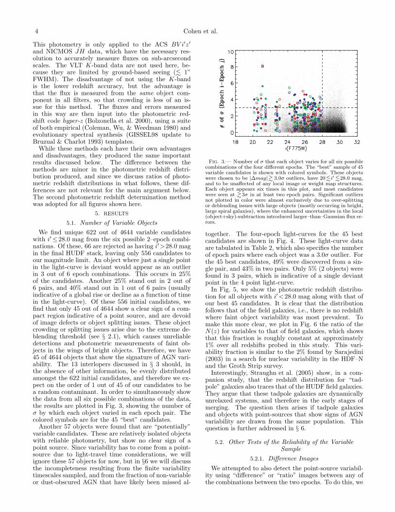
We find unique 622 out of 4644 variable candidateswith i′≤28.0 mag from the six possible 2–epoch combi-nations. Of these, 66 are rejected as having i′>28.0 magin the final HUDF stack, leaving only 556 candidates toour magnitude limit. An object where just a single pointin the light-curve is deviant would appear as an outlierin 3 out of 6 epoch combinations. This occurs in 25%of the candidates. Another 25% stand out in 2 out of6 pairs, and 40% stand out in 1 out of 6 pairs (usuallyindicative of a global rise or decline as a function of timein the light-curve). Of these 556 initial candidates, wefind that only 45 out of 4644 show a clear sign of a com-pact region indicative of a point source, and are devoidof image defects or object splitting issues. These objectcrowding or splitting issues arise due to the extreme de-blending threshold (see § 2.1), which causes unreliabledetections and photometric measurements of faint ob-jects in the wings of bright objects. Therefore, we have45 of 4644 objects that show the signature of AGN vari-ability. The 13 interlopers discussed in § 3 should, inthe absence of other information, be evenly distributedamongst the 622 initial candidates, and therefore we ex-pect on the order of 1 out of 45 of our candidates to bea random contaminant. In order to simultaneously showthe data from all six possible combinations of the data,the results are plotted in Fig. 3, showing the number ofσ by which each object varied in each epoch pair. Thecolored symbols are for the 45 “best” candidates.

Another 57 objects were found that are “potentially”variable candidates. These are relatively isolated objectswith reliable photometry, but show no clear sign of apoint source. Since variability has to come from a point-source due to light-travel time considerations, we willignore these 57 objects for now, but in §6 we will discussthe incompleteness resulting from the finite variabilitytimescales sampled, and from the fraction of non-variableor dust-obscured AGN that have likely been missed al-

Fig. 3.— Number of σ that each object varies for all six possiblecombinations of the four different epochs. The “best” sample of 45variable candidates is shown with colored symbols. These objectswere chosen to be |∆mag|& 3.0σ outliers, have 20.i′ .28.0 mag,and to be unaffected of any local image or weight map structures.Each object appears six times in this plot, and most candidateswere seen at &3σ in at least two epoch pairs. Significant outliersnot plotted in color were almost exclusively due to over-splittingor deblending issues with large objects (mostly occurring in bright,large spiral galaxies), where the enhanced uncertainties in the local(object+sky)-subtraction introduced larger–than–Gaussian flux er-rors.

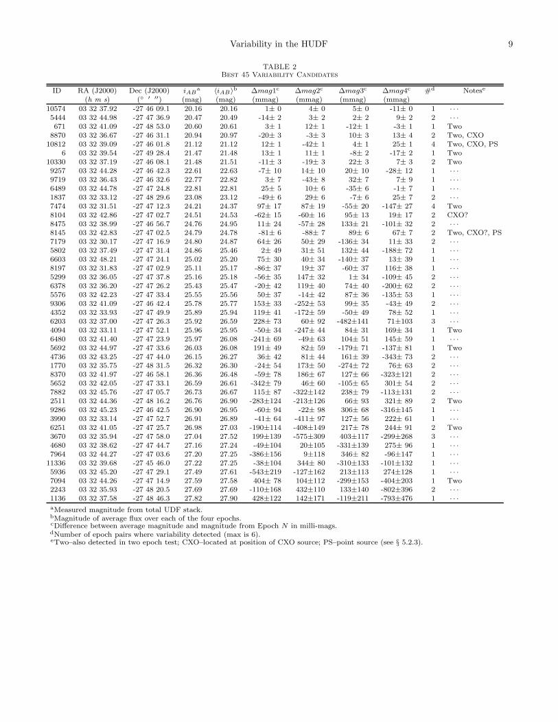
together. The four-epoch light-curves for the 45 bestcandidates are shown in Fig. 4. These light-curve dataare tabulated in Table 2, which also specifies the numberof epoch pairs where each object was a 3.0σ outlier. Forthe 45 best candidates, 49% were discovered from a sin-gle pair, and 43% in two pairs. Only 5% (2 objects) werefound in 3 pairs, which is indicative of a single deviantpoint in the 4 point light-curve.

In Fig. 5, we show the photometric redshift distribu-tion for all objects with i′<28.0 mag along with that ofour best 45 candidates. It is clear that the distributionfollows that of the field galaxies, i.e., there is no redshiftwhere faint object variability was most prevalent. Tomake this more clear, we plot in Fig. 6 the ratio of theN(z) for variables to that of field galaxies, which showsthat this fraction is roughly constant at approximately1% over all redshifts probed in this study. This vari-ability fraction is similar to the 2% found by Sarajedini(2003) in a search for nuclear variability in the HDF–Nand the Groth Strip survey.

Interestingly, Straughn et al. (2005) show, in a com-panion study, that the redshift distribution for “tad-pole” galaxies also traces that of the HUDF field galaxies.They argue that these tadpole galaxies are dynamicallyunrelaxed systems, and therefore in the early stages ofmerging. The question then arises if tadpole galaxiesand objects with point-sources that show signs of AGNvariability are drawn from the same population. Thisquestion is further addressed in § 6.

5.2. Other Tests of the Reliability of the VariableSample

5.2.1. Difference Images

We attempted to also detect the point-source variabil-ity using “difference” or “ratio” images between any ofthe combinations between the two epochs. To do this, we

Variability in the HUDF 5

0 20 40 60 80 100−1

−.5

0

.5

1

Days

∆mag

ID11336 iAB=27.22

0 20 40 60 80 100Days

ID5936 iAB=27.49

0 20 40 60 80 100Days

ID7094 iAB=27.59

0 20 40 60 80 100Days

ID2243 iAB=27.69

0 20 40 60 80 100Days

ID1136 iAB=27.82−1

−.5

0

.5

1

∆mag

ID3990 iAB=26.91 ID6251 iAB=26.98 ID3670 iAB=27.04 ID4680 iAB=27.16 ID7964 iAB=27.20−1

−.5

0

.5

1

∆mag

ID8370 iAB=26.36 ID5652 iAB=26.59 ID7882 iAB=26.73 ID2511 iAB=26.76 ID9286 iAB=26.90−1

−.5

0

.5

1

∆mag

ID4094 iAB=25.96 ID6480 iAB=25.97 ID5692 iAB=26.03 ID4736 iAB=26.15 ID1770 iAB=26.32−1

−.5

0

.5

1

∆mag

ID6378 iAB=25.43 ID5576 iAB=25.55 ID9306 iAB=25.78 ID4352 iAB=25.89 ID6203 iAB=25.92

−.4

−.2

0

.2

.4

∆mag

ID7179 iAB=24.80 ID5802 iAB=24.86 ID6603 iAB=25.02 ID8197 iAB=25.11 ID5299 iAB=25.16

−.2

−.1

0

.1

.2

∆mag

ID1837 iAB=23.08 ID7474 iAB=24.21 ID8104 iAB=24.51 ID8475 iAB=24.76 ID8145 iAB=24.79

PS

−.1

−.05

0

.05

.1

∆mag

ID6 iAB=21.47 ID10330 iAB=21.48 ID9257 iAB=22.61 ID9719 iAB=22.77 ID6489 iAB=22.81

−.04

−.02

0

.02

.04

∆mag

ID10574 iAB=20.16 ID5444 iAB=20.47 ID671 iAB=20.60 ID8870 iAB=20.94 ID10812 iAB=21.12

PS

Fig. 4.— Light curves of the 45 best candidates with signs of optical AGN variability. The vertical axes are the change in measuredmagnitudes plotted in the sense of the average minus individual measurements. The horizontal axis is the number of days since the firstmeasurement. Each panel shows the object ID number in the upper left, and the i′

ABmagnitude in the upper right. Plots are arranged

in order of decreasing flux, and the combined total flux error bars are from SExtractor. The two point sources discussed in § 5.2.3 areindicated by “PS.”

6 Cohen et al.

Fig. 5.— Photometric redshift distribution of all HUDF fieldgalaxies (solid line) and for the “best” variable candidates (dashedline) multiplied by 60× for best comparison. Photo-z’s computedusing hyperZ (Bolzonella et al. 2000) and BV i′z′JH HST datafor all galaxies with i′ .28.0 mag. The redshift distribution of thevariable objects follows that of field galaxies in general.

Fig. 6.— Percentage of HUDF objects to i′ . 28.0 AB-magshowing variable point sources as a function of photo-z. Within thestatistical uncertainties, about 1% of all HUDF galaxies show pointsource variability over the whole redshift range surveyed (0.z .5).

smoothed the image by a 5×5 and 7×7 box. For each ob-ject, a “variance map” is computed over the four epochsas follows. For each pixel, we compute the n×n box-average for both the image and the weight map. Thenwe compute the weighted standard deviation over thefour epochs for each pixel in the box-averaged images.The n×n box-size was chosen to smooth out most ofthe PSF breathing and registration issues. Even so, thisvariance image clearly had peaks in the centers of allbright objects. However, the variable candidates alsotended to stand out more than their non-variable neigh-bors. This method worked best for the brighter objects,clearly verifying 13/18 candidates with i′AB . 25 mag,but only finding ∼50% of the full i′AB .28 mag sample.While not an optimal method of detection, this ratio-method provided a good way of confirming some of theobjects whose total flux changed significantly over thefour month period. However, the total flux method re-mains our primary variable candidate detection method,

since it is most robust against ACS PSF effects.

5.2.2. Variability Between Two Deeper Epochs

Given the observing dates listed in Table 1, a natu-ral test is to combine the first and second epochs, andalso the third and fourth, giving only two independentHUDF epochs but more widely spaced in time, and witha somewhat higher signal-to-noise ratio for the variablecandidate detection. However, we expect fewer variablecandidates this way, because there are fewer epochs tocompare, and because some of the short-term variabil-ity signature is necessarily smoothed over. From this2–epoch test, 242 candidates are chosen from the errordistribution. Next this list is compared to the list of the45 best candidates from the 4-epoch search, and 12 ob-jects were found in both searches. If the list of the bestand possible candidates are combined, there are 102 can-didates, and 30 of these are recovered in the two epochtest. This test gives further confidence that at least 30%of our top candidates are truly variable objects, althoughit does not exclude any of the other ones, since those werefound when the shorter time-baselines were included.

A sample of local AGN light-curves can be used in or-der to assess the expected completeness in temporallycondensing our HUDF data from four to two epochs.The best publicly available data is that from the ex-tensive International AGN Watch1 (hereafter IAGNW;Peterson et al. 2002, and references therein). We usedtheir five IAGNW Seyferts (all with z < 0.05), whichhave B-band light-curves which best match our observedHUDF i′-band data, since the median redshift of our can-didates is zmed≃1.5. Since the rest-frame time samplingdepends on the redshifts of the HUDF objects, we re-sampled the IAGNW light-curves for a range of redshiftsbetween 0.5 < z < 5. The IAGNW data allowed for 30–40 independent 4–epoch light-curves to be created fora given redshift. These light-curves were then scaled tomatch the observed spread in ∆mag as a function of mag-nitude for our 45 HUDF candidates. A Monte Carlo testwas then run on mock catalogs that matched the samemagnitude distribution as our 45 HUDF candidates. Onaverage half of the ∼40 light-curves are found when our4–epoch variability algorithm (using same 3σ selectioncurves) is applied. The 2–epoch algorithm is then ap-plied to those mock candidates and the number that re-main variable candidates turns out to be a decreasingfunction of assumed redshift. We recover 60–70% forz . 1 and 30–40% for z & 4. However, this test relieson using 20 templates to simulate 45 objects. A visualinspection of the light-curves in Fig. 4 shows that ideallya larger number of local templates is needed for a fairtest. Nonetheless, this limited test that is possible withthe available IAGNW data – when taken at face value –may be an indication that as many as one-third of our45 candidates are potentially false positives, although itis equally likely that the small number of local test tem-plates are not truly representative of the distant HUDFvariability sample. Hence, we believe that the reliabil-ity of our faint HUDF variability sample is likely largerthan 67%, but we will not be able to definitively say for

1 Tabulated data from the InternationalAGN Watch can be found at the URLhttp://www.astronomy.ohio-state.edu/$\sim$agnwatch/

Variability in the HUDF 7

sure without more local light-curve templates that bestmatch the high-z variable objects.

5.2.3. Other Wavelengths

Since the UDF is in the Chandra Deep Field–South(CDFS; Rosati et al. 2002), there exists deep X-ray datain this field, and these data are ideal for detecting AGN.Within the UDF, there are 16 Chandra sources (Koeke-moer et al. 2005, in preparation), and we detect fourof these as variable in the optical. One of these is amid-type spiral with i′=21.24 mag, that is a member ofa small group of apparently interacting galaxies. Inter-estingly, this object’s total flux varied by less than 1%,but since it was one of the brightest objects in the sam-ple, its variability was clearly detected at &3.0σ signifi-cance. Two of the others are optical point sources, show-ing little or no visible host galaxy, with i′ = 21.12 magand i′ = 24.79 mag. They both have measured spectro-scopic AGN emission-line redshifts from the GRism ACSProgram for Extragalactic Science survey (GRAPES;Pirzkal et al. 2004) at z ≃ 3. Our BV i′z′JH photomet-ric redshifts put them at z = 2.6 and z = 2.9 respec-tively, which is rather good given that these few brighterAGN are the ones that are most dominated by a non-stellar power-law SED. The fourth candidate is barelydetected in any of the ACS bands, and would have beeneliminated as a spurious candidate had it not been co-incident with the Chandra source, and is clearly a vi-able object in the VLT K-band image. The detectionof 25% of the Chandra sources as optically variable inthe HUDF data shows that the method employed hereis a reliable way of finding the AGN that are not heav-ily obscured. Paolillo et al. (2004) find that > 90% ofthe studied CDFS X-ray sources with adequate photonstatistics show X-ray variability, and a future compari-son of the X-ray and optical variability amplitudes couldprovide insight into the physical mechanism that is re-sponsible for this variability.

5.3. Possible Sources of Incompleteness in the VariableAGN Sample

In summary, we found 45 plausibly variable objectswith some caveats, and this number may be as high as102 if the “possible” variable candidates are included.Hence, the true variability fraction on timescales of afew months (rest-frame timescale few weeks to a month)is no more than about 1–2% of all HUDF field galaxies.Except for variable stars such as SNe and novae, this vari-ability is most likely due to an AGN given the timescalesand distances involved. Strolger & Riess (2005) foundonly one moderate redshift SNe in the HUDF, and thusSNe cannot be a significant source of contamination ofthe present sample.

Two other possible source of incompleteness in thevariability study must be addressed first. Non-variableAGN, or AGN that only vary on timescales much longerthan 4 months, or optically obscured AGN would nothave been detected with the current UV–optical vari-ability method. Sarajedini et al. (2003a) had epochs 5–7years apart, and found 2% of the objects to be variable.It is thus possible that the currently sampled times-scaleshorter than 4 months missed about a factor 2 of all AGNthat are only variable on longer time-scales.

A factor of three of the brighter AGN may have beenmissed, since their UV–optical flux may be obscured bya dust-torus (Barthel 1989). In the AGN unification pic-ture, AGN cones are two-sided and their axes are ran-domly distributed in the sky, so that an average coneopening angle of ω implies that a fraction 1–sin(ω) of allAGN will point in our direction. If ω≃45◦ (e.g., Barthel1989), then every optically detected AGN (QSO) rep-resents 3–4 other bulge-dominated galaxies, whose AGNreflection cone didn’t shine in our direction. Hence, theirAGN may remain obscured by the dust-torus. Such ob-jects would be visible to Chandra in the X-rays or toSpitzer at mid-IR wavelengths, although the availableChandra and Spitzer data are not nearly deep enoughto detect all HUDF objects to AB =28 mag. (Reachingthese depths is prohibitive in Chandra and Spitzer inte-gration times, and requires the next generation of X-rayand IR telescopes, such as Generation-X and JWST).At brighter flux limits, Spitzer did indeed recently finda significant fraction of dust-obscured AGN not seen inUV-optical surveys (Urry et al. 2004). In the AGN uni-fication picture, the incompleteness in UV–optically se-lected samples due to the dust-obscuring torus would beas large as a factor of 3–4 (Treister et al. 2004).

6. DISCUSSION AND CONCLUSIONS

6.1. Fraction of Variable AGN found

Interestingly, Straughn et al. (2005) show, in a com-panion study, that the redshift distribution for “tadpole”galaxies also traces that of the HUDF field galaxies for0.1 . z . 4.5. They argue that these tadpole galaxiesare dynamically unrelaxed systems, and therefore in theearly stages of merging. The question then arises if tad-pole galaxies and objects with point-sources that showsigns of AGN variability are drawn from the same popu-lation. At any given redshift, Straughn et al. (2005) findthat about 6% of all HUDF galaxies appear as tadpoles,and they conclude that tadpole galaxies are good tracersof the process of galaxy assembly.

Together with the factor of & 2 incompleteness inthe HUDF variability sample due to the limited time-baseline sampled thus far, the actual fraction of weakAGN present in these dynamically young galaxies maybe a factor of &6–8× larger than the 1% variable AGNfraction found through variability in the HUDF. Hence,perhaps as many as &6–8% of all field galaxies may hostweak AGN, only ∼ 1% of which we found here, and an-other & 1% could have been found if longer time-baselinehad been available. The other factor of 3–4× of AGN arelikely missing because they are optically obscured, re-quiring the next generation of X-ray and IR telescopes.

6.2. AGN feeding timescales compared to galaxy mergertimescales

We now consider if the current variability dataset canconstrain the merging rate of SMBHs, assuming thatSMBHs formed during hierarchical mergers of galax-ies containing less massive SMBHs, and if signatures ofgalaxy mergers could be related to variable AGNs. Putanother way, can signatures of galaxy merging be relatedto our variable AGN candidates?

A closer inspection of our data reveals that only1 or perhaps 2 of the variable candidates resemble

8 Cohen et al.

the tadpole galaxies of Straughn et al. (2005). Re-cent state-of-the-art hierarchical models have suggestedthat the AGN-phase only occurs in the later stagesof a galaxy merger, and well after it appears in thetadpole phase (Springel, Di Matteo, & Hernquist 2005;di Matteo, Springel, & Hernquist 2005). These modelsalso predict that the AGN will likely only be visible wellafter (&1 Gyr) the merger induced star-formation hasdied down, implying that the fraction of dynamicallyyoung tadpoles that are expected to already show activeAGN properties is relatively small. The small overlapbetween the two populations that we observe does thusnot exclude the possibility that faint object variabilityis tracing the growth of SMBHs. However, this SMBHgrowth can only be constrained indirectly from the vari-ability data, and a more detailed discussion of the con-nection between mergers and AGN activity is given inStraughn et al. (2005) and references therein.

Given the importance of understanding the growth andorigin of SMBHs, several lessons can be learned from thiswork in order to better design future studies of this type.The time-spacing of the HUDF observations –althoughas good as possible given scheduling constraints–was notideal for this type of study. It is critical to re-visitthe HUDF with HST, with the observations optimized

for a faint-object variability study, including coveringtime-scales of a few years. It is also essential to plandeeper surveys at longer wavelengths with the JWST.The JWST photometric and PSF stability are crucial inthis regard, as many of our HUDF objects show signifi-cant variability of less than a few percent in flux. Also, alimiting factor in our results is the breathing of the PSF,along with image noise due to correcting the geometricdistortion of ACS and slight variations of the PSF acrossthe field. Therefore, JWST must have design specifi-cations that are capable of meeting these requirementsin order to permit faint object variability studies to bedone.

We acknowledge the support from the NASA grantsHST-GO-09793.*, awarded by STScI, which is operatedby AURA for NASA under contract NAS 5-26555. Thiswork was funded in part by NASA JWST grant NAG5-12460 (to RAW). This work benefited from fruitful dis-cussions with Drs. M. Corbin, H. Ferguson, L. Hern-quist, R. Jansen, V. Sarajedini, and many others. Wealso thank the anonymous referee for helpful suggestionsthat improved the paper.

Facility: HST(ACS).

REFERENCES

Barthel, P. D. 1994, ApJ, 336, 606Beckwith, S. et al. 2005, AJ, in prep.Bertin, E. & Arnouts 1996, A&AS, 117,393Bolzonella, M., Miralles, J.-M., & Pello, R. 2000, A&A, 363,476Bouwens, R. J, et al. 2004, ApJ, 616, 79Bruzual, G. & Charlot, S. 1993 ApJ, 405, 538Coleman, G. D., Wu, C.-C., & Weedman, D. W. 1980, ApJS, 43,

393di Matteo, T., Springel, V., & Hernquist, L. 2005, Nature, 433, 604Ferrarese, L. & Ford, H.C. 2004, Space Sci. Rev., 116, 523Heymans, C., et al. 2005, MNRAS, 361, 160Koekemoer, A. M., Fruchter,A. S., Hook, R., & Hack, W. 2002,

in Proceedings of the 2002 HST Calibration Workshop, ed. S.Arribas, A. Koekemoer, and B. Whitmore (Baltimore: SpaceTelescope Science Institute), 339

Kogut, A., et al. 2003, ApJS, 148, 161Kormendy, J. & Richstone, D. 1995, ARA&A, 33, 581Kormendy, J. & Gebhardt, K. 2001, in AIP Conf. Proc. 586: 20th

Texas Symposium on Relativistic Astrophysics, 363Madau, P., & Rees, M. 2001, ApJ, 551, L27

Magorrian, J., Tremaine, S., & Richstone, D. 1998, AJ,115, 2285Paltani, S., & Courvoisier, T. J.-L. 1994, A&A, 291, 74Paolillo, M., Schreier, E. J., Giacconi, R., Koekemoer, A. M., &

Grogin, N. A. 2004, ApJ, 611, 93Pirzkal, N., et al. 2004, ApJS, 154, 501Peterson, B. M., et al. 2002, ApJ, 581, 197Rosati, P., et al. 2002, ApJ, 566, 667Sarajedini, V. L., Gilliland, R. L. & Kasm, C. 2003, ApJ, 599, 173Sarajedini, V. L., 2003, MmSAI, 74, 957Silk, J., & Rees, M. 1998, A&A, 331, L1Springel,V., Di Matteo, T., & Hernquist, L. 2005, ApJ, 620, 79Straughn, A. N., Cohen, S. H., Ryan, R. E., Hathi, N. P., &

Windhorst, R. A. 2005, this volumeStrolger, L.-G., & Riess, A. G. 2005, preprint (astro-ph/0503093)Thompson, R. I., et al. 2005, AJ, 130, 1Treister, E., et al. 2004, ApJ, 616, 123Urry, C. M., et al. 2004, BAAS, 205.6209Yan, H., & Windhorst, R. A. 2004, ApJ, 612, 93

Variability in the HUDF 9

TABLE 2Best 45 Variability Candidates

ID RA (J2000) Dec (J2000) iABa 〈iAB〉b ∆mag1c ∆mag2c ∆mag3c ∆mag4c #d Notese

(h m s) (◦ ′ ′′) (mag) (mag) (mmag) (mmag) (mmag) (mmag)

10574 03 32 37.92 -27 46 09.1 20.16 20.16 1± 0 4± 0 5± 0 -11± 0 1 · · ·5444 03 32 44.98 -27 47 36.9 20.47 20.49 -14± 2 3± 2 2± 2 9± 2 2 · · ·671 03 32 41.09 -27 48 53.0 20.60 20.61 3± 1 12± 1 -12± 1 -3± 1 1 Two

8870 03 32 36.67 -27 46 31.1 20.94 20.97 -20± 3 -3± 3 10± 3 13± 4 2 Two, CXO10812 03 32 39.09 -27 46 01.8 21.12 21.12 12± 1 -42± 1 4± 1 25± 1 4 Two, CXO, PS

6 03 32 39.54 -27 49 28.4 21.47 21.48 13± 1 11± 1 -8± 2 -17± 2 1 Two10330 03 32 37.19 -27 46 08.1 21.48 21.51 -11± 3 -19± 3 22± 3 7± 3 2 Two9257 03 32 44.28 -27 46 42.3 22.61 22.63 -7± 10 14± 10 20± 10 -28± 12 1 · · ·9719 03 32 36.43 -27 46 32.6 22.77 22.82 3± 7 -43± 8 32± 7 7± 9 1 · · ·6489 03 32 44.78 -27 47 24.8 22.81 22.81 25± 5 10± 6 -35± 6 -1± 7 1 · · ·1837 03 32 33.12 -27 48 29.6 23.08 23.12 -49± 6 29± 6 -7± 6 25± 7 2 · · ·7474 03 32 31.51 -27 47 12.3 24.21 24.37 97± 17 87± 19 -55± 20 -147± 27 4 Two8104 03 32 42.86 -27 47 02.7 24.51 24.53 -62± 15 -60± 16 95± 13 19± 17 2 CXO?8475 03 32 38.99 -27 46 56.7 24.76 24.95 11± 24 -57± 28 133± 21 -101± 32 2 · · ·8145 03 32 42.83 -27 47 02.5 24.79 24.78 -81± 6 -88± 7 89± 6 67± 7 2 Two, CXO?, PS7179 03 32 30.17 -27 47 16.9 24.80 24.87 64± 26 50± 29 -136± 34 11± 33 2 · · ·5802 03 32 37.49 -27 47 31.4 24.86 25.46 2± 49 31± 51 132± 44 -188± 72 1 · · ·6603 03 32 48.21 -27 47 24.1 25.02 25.20 75± 30 40± 34 -140± 37 13± 39 1 · · ·8197 03 32 31.83 -27 47 02.9 25.11 25.17 -86± 37 19± 37 -60± 37 116± 38 1 · · ·5299 03 32 36.05 -27 47 37.8 25.16 25.18 -56± 35 147± 32 1± 34 -109± 45 2 · · ·6378 03 32 36.20 -27 47 26.2 25.43 25.47 -20± 42 119± 40 74± 40 -200± 62 2 · · ·5576 03 32 42.23 -27 47 33.4 25.55 25.56 50± 37 -14± 42 87± 36 -135± 53 1 · · ·9306 03 32 41.09 -27 46 42.4 25.78 25.77 153± 33 -252± 53 99± 35 -43± 49 2 · · ·4352 03 32 33.93 -27 47 49.9 25.89 25.94 119± 41 -172± 59 -50± 49 78± 52 1 · · ·6203 03 32 37.00 -27 47 26.3 25.92 26.59 228± 73 60± 92 -482±141 71±103 3 · · ·4094 03 32 33.11 -27 47 52.1 25.96 25.95 -50± 34 -247± 44 84± 31 169± 34 1 Two6480 03 32 41.40 -27 47 23.9 25.97 26.08 -241± 69 -49± 63 104± 51 145± 59 1 · · ·5692 03 32 44.97 -27 47 33.6 26.03 26.08 191± 49 82± 59 -179± 71 -137± 81 1 Two4736 03 32 43.25 -27 47 44.0 26.15 26.27 36± 42 81± 44 161± 39 -343± 73 2 · · ·1770 03 32 35.75 -27 48 31.5 26.32 26.30 -24± 54 173± 50 -274± 72 76± 63 2 · · ·8370 03 32 41.97 -27 46 58.1 26.36 26.48 -59± 78 186± 67 127± 66 -323±121 2 · · ·5652 03 32 42.05 -27 47 33.1 26.59 26.61 -342± 79 46± 60 -105± 65 301± 54 2 · · ·7882 03 32 45.76 -27 47 05.7 26.73 26.67 115± 87 -322±142 238± 79 -113±131 2 · · ·2511 03 32 44.36 -27 48 16.2 26.76 26.90 -283±124 -213±126 66± 93 321± 89 2 Two9286 03 32 45.23 -27 46 42.5 26.90 26.95 -60± 94 -22± 98 306± 68 -316±145 1 · · ·3990 03 32 33.14 -27 47 52.7 26.91 26.89 -41± 64 -411± 97 127± 56 222± 61 1 · · ·6251 03 32 41.05 -27 47 25.7 26.98 27.03 -190±114 -408±149 217± 78 244± 91 2 Two3670 03 32 35.94 -27 47 58.0 27.04 27.52 199±139 -575±309 403±117 -299±268 3 · · ·4680 03 32 38.62 -27 47 44.7 27.16 27.24 -49±104 20±105 -331±139 275± 96 1 · · ·7964 03 32 44.27 -27 47 03.6 27.20 27.25 -386±156 9±118 346± 82 -96±147 1 · · ·

11336 03 32 39.68 -27 45 46.0 27.22 27.25 -38±104 344± 80 -310±133 -101±132 1 · · ·5936 03 32 45.20 -27 47 29.1 27.49 27.61 -543±219 -127±162 213±113 274±128 1 · · ·7094 03 32 44.26 -27 47 14.9 27.59 27.58 404± 78 104±112 -299±153 -404±203 1 Two2243 03 32 35.93 -27 48 20.5 27.69 27.69 -110±168 432±110 133±140 -802±396 2 · · ·1136 03 32 37.58 -27 48 46.3 27.82 27.90 428±122 142±171 -119±211 -793±476 1 · · ·aMeasured magnitude from total UDF stack.bMagnitude of average flux over each of the four epochs.cDifference between average magnitude and magnitude from Epoch N in milli-mags.dNumber of epoch pairs where variability detected (max is 6).eTwo–also detected in two epoch test; CXO–located at position of CXO source; PS–point source (see § 5.2.3).