DRAFT - TU Berlinpage.math.tu-berlin.de/~gunn/Documents/Papers/GAforCGTRaw.pdf · DRAFT 3 Geometric algebra for euclidean space Since we are interested here in practical applications,

DRAFT

Geometric Algebra: a tutorial for graphics programmers

Charles Gunn∗

Technical University BerlinInstitute for Mathematics 8-3

10623 Berlin [email protected]

Abstract

Most computer graphics developers are familiar with the use of unit quaternions torepresent rotations in euclidean space. A smaller number know of the existence of dualquaternions, that also allow representation of translations in the same way. Even fewerknow that there exists a further algebraic structure (which contains these quaternionalgebras as sub-algebras) which provides an even richer environment for doing geom-etry, and demonstrates significant advantages over the traditional linear algebra andvector analysis approach. This structure, projective geometric algebra, models in acompact, coordinate-free form both metric and incidence relationships in euclideanspace. Points, lines and planes are handled in a uniform way, and there is no distinc-tion between the representation of operators and operands. After a quick introduction,we demonstrate the power of this algebra to handle familiar geometric constructions.We then move on to representing arbitrary euclidean isometries (including reflections,translations, and screws) using sandwich operations in the algebra, obtaining in thisway a new and enlightening perspective on the quaternions and dual quaternions. Weshow how classical vector analysis can be found within the ideal plane of the algebra.We close with a sketch of the elegant form which kinematics and rigid body mechanicstakes in this framework.

1 Doing geometry on a computer

What is the “right” way to represent geometry for a computer? The traditional linearalgebra approach is point-centric and dualistic. “Point-centric” since geometric computa-tions involving lines or planes must be handled separately; “dualistic” since operands andoperators are distinct: the translation by a vector (a matrix) is different from the vectoritself. While the worlds handled by computer graphics become more and more complex,this basic representation has not changed since the pioneer days. Must this be so?

∗Research supported by Matheon Center for Key Technologies

1

DRAFT

We present in this article projective geometric algebra (PGA) a system for doing ge-ometry which is entity-neutral (meaning points, lines and planes are equal citizens), andmonistic in the sense that the same entity can be either operand or operator, depending oncontext. It can be simply described and implemented; it is practical and computationallyefficient. It is compatible with the traditional approach; implementors can transition grad-ually from the prevailing linear algebra + vector analysis approach to PGA. Furthermore,its monistic nature means that all expressions have intuitive geometric meanings, henceprogramming of complex tasks is simplified. It has deep mathematical roots in the 19th

century research of Grassmann, Klein, Clifford, and Study; the novelty of our approach isto bring together existing results into a modern formulation, blow some dust away from theold sources, as it were, and allow them to shine forth again in their original glory. Quater-nions and dual quaternions provide a natural bridge for computer graphics practitioners tounderstand PGA, so we begin with a brief review of how these algebraic structures havefound acceptance in computer graphics.

2 Like (dual) quaternions, only better

Recall that for a unit quaternion

h := cos (α) + sin (α)(ai + bj + ck)

and an imaginary quaternionX = xi + yj + zk

representing a point in E3, the rotation around the axis (a, b, c) by the angle 2α is givenby the “sandwich” operation

X→ hXh

(where h is the quaternion conjugate of h). A similar formulation using dual quaternionsallows translations to be represented similarly.

These sandwich operations are also present in PGA, as a subgroup of the full isometrygroup of euclidean space that includes reflections (both in planes and the less well-knownpoint reflections). We will see below in Sect. ?? that the quaternions and dual quaternionsare generated naturally by the reflections in planes. In the process we believe that themystery surrounding dual numbers can be transformed into geometric insight.

Qualitatively, the main difference between PGA and these quaternion algebras is thatPGA is a graded algebra, that is, can be written as the direct sum of a finite set ofelements of integer grade. The grade-k elements provide a faithful representations of then − k-dimensional subspaces of euclidean n-space, enabling a rich variety of geometricoperations involving the points, lines, and planes of E3, something not at all possible withquaternions alone. See Sect. ?? for examples in the euclidean plane.

2

DRAFT

3 Geometric algebra for euclidean space

Since we are interested here in practical applications, we dispense with a traditional expo-sition of projective geometric algebra and begin immediately with the necessary definitionsbefore turning to some practical examples of its use. Readers who would like a moredetailed introduction can consult [3], [4], or [2].

3.1 Geometric product on basis vectors

The geometric algebra studied here is a graded algebra consisting of vectors of gradesrunning from 0 to 4, each grade representing a particular type of geometric entity, asshown in the following tabled. The algebraic structure is defined by the geometric product,which is an associative product defined on any pair of elements in the algebra. We describethis geometric product in more detail below

An element that can be written as the geometric product of k 1-vectors is called ak-blade. A sum of k-blades is a k-vector. Such an element is said to have grade k; thek-vectors form a vector space written P(

∧k R4∗). A general element of the algebra is amultivector and is a sum of k-vectors for mixed k’s. The grades arise from the geometricproduct as follows.

Grade 0 1 2 3 4

Type Scalars Planes Lines Points Pseudoscalars

Grade-1 The basis 1-vectors (e0, e1, e2, e3) represent the four coordinate planes1 w = 0,x = 0, y = 0, and z = 0, resp. They satisfy e20 = 0, e21 = e22 = e23 = 1. e0 is called theideal plane. Readers familiar with homogeneous coordinates in computer graphicsperhaps know it as the “plane at infinity”. A general 1-vector is a linear combinationof the basis 1-vectors: a :=

∑i aiei and represents the plane a1x+a2y+a3z+a0 = 0.

Grade-2 Their pair-wise products eij := eiej for i 6= j form a basis of the 2-vectors andsatisfy eij = −eji. It then follows that e20j = 0 and otherwise e2ij = −1. Theyrepresent the six lines of intersection of the coordinate planes. The lines e0j are ideallines, since they lie in the ideal plane. A general 2-vector is a weighted sum of six ofthese basis vectors:

Π = p01e01 + p02e02 + p03e03 + p12e12 + p31e31 + p23e23

Note that the term involving e31 is chosen instead of e13. Not every 2-vector repre-sents a line; necessary and sufficient is the so-called Plucker condition on the coordi-nates of a 2-vector

∑aijeij that a01a23+a02a31+a03a12 = 0. When it is satisfied the

1It’s not possible to construct euclidean space by beginning with points; one obtains a different metricspace. For details see [3].

3

DRAFT

resulting coordinates are the Plucker coordinates for the line. We somewhat sloppilyalso apply the term for the coordinates of any 2-vector. A 2-vector which representsa line is called simple. Non-simple 2-vectors arise for example as the sum of two skewlines. Line geometry will be discussed in more detail later.

Grade-3 The 3-vectors represent points. The basis tri-vectors are defined by

E0 = e123 := e1e2e3, E1 := e032, E2 := e013, E3 := e021

Each represents the intersection point of three of the four basis planes. One can easilycalculate E2

0 = 1, otherwise E2i = 0. E0 is the origin; otherwise Ei is an ideal point

(in the x−, y−, and z− directions, resp.) since it lies in the ideal plane. These arehomogeneous coordinates for euclidean space, introduced originally as coordinatesfor projective geometry. Hence the name “projective geometric algebra”.

Grade 4 The pseudoscalar I := e0e1e2e3 is a basis of the one-dimensional space of 4-vectors and satisfies I2 = 0. Multiplication by I is a grade-reversing map of thealgebra. It maps any euclidean plane to its normal direction, an ideal point; andmaps all euclidean points to the ideal plane. Since I2 = 0, this operation is non-invertible. Such a pseudoscalar is called degenerate and is often in the literaturepresented in a negative light since it prevents certain simplications of formulae, noneof which however have serious consequences. On the positive side, it is mirrors themetric properties of euclidean geometry faithfully and in this sense is an indispensiblefeature of the algebra.

Grade 0 A 0-vector is a scalar. Scalars and pseudo-scalars commute with everything.They form a sub-algebra called the dual numbers.2

3.2 Terminology

We introduce some conventions for naming geometric entities, and review some notationfor geometric algebra which will come in handy in the sequel:• a, b, etc., (small Roman letters) refer to 1-vectors (planes),• Π, Σ, etc., (large Greek letters) refer to 2-vectors (lines and line complexes)3, and• P, Q, etc. (large Roman letters) refer to 3-vectors (points).• X refers to an arbitrary k-vector.• a 2-vector is also called a bivector, and a 3-vector, a trivector.• 〈M〉k is the restriction of the multivector M to its grade-k part. M =

∑k 〈M〉k.

• The reversal involution X reverses the order of all products of 1-vectors in the algebra.

An official name for PGA. The geometric algebra with the above properties is writtenP(R∗3,0,1), in words, the “real dual projective Clifford algebra with signature (3, 0, 1)”. Thepieces of this imposing description have the following meanings:

2The name is due to Eduard Study who discovered many results regarding projective geometric algebrain his magnus opus [7].

3This convention goes back to Felix Klein’s original papers devoted to line geometry [5]

4

DRAFT

“real” The scalars are elements of R.“dual” The 1-vectors represents planes, not points.“projective” Homogeneous coordinates are used for all entities.“signature(3,0,1)” The squares of the basis 1-vectors include 3 positive values, 0 negative

ones, and 1 zero.

3.3 Inner and outer products

Recall that the quaternion product of two imaginary quaternions a := axi + ayj + azk andb := bxi + byj + bzk decomposes naturally as an inner product and a cross product:

ab = −a · b + a× b

where the references on the RHS refer to the quaternions as vectors in R3. The formeris a symmetric product (since b · a = b · a), while the latter is anti-symmetric (sincea× b = −b× a).

A similar decomposition occurs in geometric algebra. The geometric product of a k-vector and a m-vector decomposes naturally into pieces, each of a different grade. Forexample, begin by considering the geometric product ab of two 1-vectors a and b. Usingthe relations introduced above along with linearity to calculate, one obtains that ab =〈ab〉0+〈ab〉2, i. e., the product consists of a scalar plus a bivector. We define a·b := 〈ab〉0and the a ∧ b := 〈ab〉2. The former is called the inner product and is symmetric. Thelatter is called the wedge, or outer, product and is anti-symmetric. Summing up,

ab := a · b + a ∧ b

Exercise: show that a·b is the traditional euclidean inner product of the normal directionsof the two planes; and a ∧ b is the intersection line of the two planes.

One can proceed in the same way for the geometric product of a k-vector a and anm-vector b for other values of k and m. We define the lowest grade part of the product tobe the inner product a ·b; and the highest grade part (when k+m ≤ 4) to be the outer, orwedge, product a∧b. There are only two choices of k and m which contain another grade;we skip the details in this introductory treatment. Exercise: show the lowest grade whichcan occur in the geometric product ab is |k−m|, the highest is k+m, and the others are|k−m|+2, ..., k+m−2. Hint: write the factors as sums of products of the ei and considerhow cancellations can occur.

The wedge product of a k- and m-blade is a k +m-vector representing their geometricmeet (only non-zero when the two blades are linearly independent as plane entities, whichimplies k + m ≤ 4). When non-zero, it is the highest-grade part of the product. Thevee or dual wedge of a k- and m-blade, written ∨, is a ((k + m) − 4)-vector representingtheir geometric join (only non-zero when the two blades are linearly independent as pointentities, which implies k +m ≥ 4).

5

DRAFT

3.4 Normalizing

One of the nice properties of the geometric product is that for many important types ofgeometric entities X, X2 is a scalar. This is the case for 1-vectors, simple 2-vectors, and3-vectors in our algebra. We define a euclidean plane to be one that satisfies a2 > 0.Similarly a euclidean line is a simple 2-vector which satisfies Π2 < 0, and a euclidean pointP satisfies P2 > 0. We sometimes use proper as a synonym for euclidean.

Just like in vector analysis, it is often useful to work with normalized elements. Fromthe definitions above it’s clear that euclidean points, lines, and planes have non-zero, scalarsquare. Hence it is always possible to normalize them to satisfy X2 = ±1. In general wedefine the norm of a k-vector X as ‖X‖ =

√|X2|. A normalized 1-vector is characterized

by the condition that (a1, a2, a3) is a unit normal vector to the plane. A normalized pointis one whose E0 coordinate is 1, that is, the coordinates have been dehomogenized. Anormalized proper line satisfies Π2 = −1. Ideal elements, on the other hand, alwayssatisfy ‖X‖ = 0.

Normalized euclidean elements satisfy X−1 = ±X, i. e., they are their own inverses orthe negative of their own inverses.

It’s not strictly possible to normalize pseudoscalars since I2 = 0. But since the vectorspace of pseudoscalars is 1-dimensional, the magnitude of a pseudoscalar has well-definedscalar multiple of I, and we write ‖X‖ to represent this scalar.

3.5 Free vector ∼ ideal point

The points of the ideal plane a∞ are characterised by the condition a0 = 0. On the otherhand, normalized euclidean points have a0 = 1. Hence for two such points P and Q,P − Q ∈ a∞. In traditional vector analysis, the difference of two euclidean points is afree vector. This leads to the question, do the points of a∞ provide a good model forthe free vectors? A full discussion lies outside the scope of this tutorial (see §4.4.4 of[2] for more), but the short answer is an emphatic “Yes!” The key step to establishingthis is to introduce a different inner product on the ideal plane than the one used foreuclidean points, so that the inner product of two ideal points a1E1 + a2E2 + a3E3 andb1E1 + b2E2 + b3E3 is the traditional vector dot product a1b1 + a2b2 + a3b3. This is notso strange as it may sound, since the plane a∞ is not involved in the limiting process thatleads to the degenerate signature (3, 0, 1); one obtains the desired inner product by leavingthe original inner product unchanged.4

3.6 Playground: the euclidean plane

Although our goal is geometry in euclidean space, it is of interest didactically to reduce thedimension by one and consider PGA for the euclidean plane P(R∗2,0,1). Then the 1-vectors

4For a full description of the Cayley-Klein construction involved, see §4.4 of [2].

6

DRAFT

represent lines, the 2-vectors represent points, and the pseudoscalar is a 3-vector. Unlessotherwise noted, we assume all geometric elements are normalised. Fig. 1 shows a varietyof aspects of the geometric product in this case.

We have already discussed the geometric product of two 1-vectors, in this case, the twolines a and b. The inner product a · b is the cosine of the angle between the two lines.The wedge product a ∧ b is the intersection point of the two lines. Multiplying a by thepseudoscalar I produces the ideal point in the perpendicular direction to a.

Exercise. Show that if two lines a and b intersect in a point P at an angle of θ, then

ab = cos θ + sin θP

bbI

P

Q

Q

P v Q

P x Q

a .||a Q|| v

||P v Q||

a b v a(Q a)a .

cos (a b) .-1

Figure 1: A graphical representation of selected geometric products between various k-blades in the euclidean algebra P(R∗2,0,1). Points and lines are assumed to be normalized.Ideal points are drawn as vectors, distances indicated by norms.

Product of a line and a point. What about the geometric product of a line a and apoint Q? We have

aQ = a ·Q + a ∧Q

a ·Q is a line through Q perpendicular to a. a ∧Q is a multiple of the pseudoscalar. Infact, ‖a ∧ Q‖ = d(a,Q), the distance of Q to a. Already in this example one sees thatP(R∗2,0,1) provides a powerful and coordinate-free calculus for euclidean geometry in theplane.

7

DRAFT

Magic or logic?. Why does a ·Q produce exactly the line through Q perpendicular to a?It helps perhaps to think a bit dually in the sense of projective geometry. That is, insteadof considering Q qua point, consider it as the set of lines passing through Q. (This is nodifferent than thinking of a line a as the set of points which are lie on a, a mental picturewhich seems quite natural.) This set of lines is known as a line pencil and can be given anorthogonal basis in many ways. The operation a ·Q essentially removes the line throughQ parallel to a, leaving the single element perpendicular to a. This is the general principleinvolved in the “contractions” (grade-lowering) products of geometric algebra and can beused to understand most of the sub-products which appear.

Exercise. Show that (a ·Q)a represents the orthogonal projection of Q onto a, that is,the point of a closest to Q.

Product of two points. The geometric product of two points P and Q consists of twoparts, a scalar P·Q and a point P×Q. As noted above, P·Q = 1, so is quite uninformative.P×Q is the commutator product PQ−QP. A full discussion of the commutator productis not possible in this tutorial; the inner, outer, and commutator products suffice to expressthe geometric product as the sum of single grades (in dimension 2 and 3). In this caseP×Q is the ideal point in the perpendicular direction to the line joining P and Q. Thisjoining line itself is obtained in the algebra by P ∨ Q, that is, it does not arise in thegeometric product, only in the dual wedge product ∨, introduced above. An importantfact is ‖P ∨Q‖ = d(P,Q): the norm of the joining line is the euclidean distance betweenthe two points .

Exercise. What happens to the geometric product when one or both of the points isideal?

3.7 Isometries in the euclidean plane using PGA

3.7.1 Reflections in lines

We indicated above that sandwich operators exist in P(R∗2,0,1) which implement euclideanisometries. Here we want to show how to find them. Consider the product −aPa fornormalized euclidean a and P.

−aPa = −(aP)a

= −(a ·P + a ∧P)a

= −(a ·P)a− (a ∧P)a

On the other hand,

P = a2P = a(aP)

= a(a ·P + a ∧P)

= −(a ·P)a + (a ∧P)a

8

DRAFT

The last line is obtained by calculating the commutation relations obtained by shifting thea from the left to the right. By the exercise above, (a ·P)a is the orthogonal projection of Discuss how

to calculatecommu-tationrelations.

P onto a while (a ∧P)a is a vector V⊥ perpendicular to a of length d(a,Q).

a

X

aXa

Figure 2: Reflection generated by sandwich operation with line a.

By subtracting the two equations above we obtain

P− (aPa) = 2V⊥

This expresses geometrically the condition that aPa is the reflection of the point P in theline a. We write this sandwich operation for brevity in functional notation as aXa =: a(X).

Alternative derivation. It makes better sense to show that aba is a reflection of theline b in the line a since from this, the previous result follows immediately. Indeed, writeP as the wedge of two perpendicular lines b ∧ b′ = bb′ − b · b′ = bb′ and then calculate

−aPa = −a(bb′)a

= −(aba)(ab′a)

= −(aba) ∧ (ab′a)

= (ab′a) ∧ (aba)

The next-to-last step follows from the fact that the reflections of the two lines b and b′ areperpendicular when the two lines are perpendicular. The last step uses the anti-symmetryof the wedge product – we flip the order of b and b′ so that the reflected lines intersect ina positive angle, yielding a normalized point (without flipping the wedge has homogeneouscoordinate -1). Since a reflection preserves incidence, the RHS of the last equation must What is ho-

mogeneouscoordinateand why isit -1?

be the reflection of the intersection point of b and b′, which by assumption is P.

Exercise. Show that aba is a reflection of the line b in the line a. Hint: Proceed as abovebut use the decomposition for the product of two 1-vectors, interpreted geometrically.

9

DRAFT

3.7.2 Rotations around points

We’ve established that a euclidean reflection is obtained by aXa for a 1- or 2-vector X.It’s a short step to rotations around a point. To write a sandwich operation that expressesa rotation around a point P by an angle θ, find two lines a and b that pass through P

and meet at and angle ofθ

2(measured from a to b). Then consider the product b(aXa)b.

This is the reflection in the line a followed by reflection in the line b. By school geometrywe know this is then a rotation of θ around the intersection point of a and b, i.e., aroundP, as desired.

We write the rotation sandwich operation then as

X→ RXR

where R := ba and R is the reversal involution introduced above (needed since the orderof the lines is reversed on the two sides of X). The element R is called a rotor. We canassume (as is here the case) that it is normalized so that RR = 1.

Alternative derivation using exponentials. It’s possible to derive the same resultdirectly from the input data P and θ without having to find two lines. Consider the

formal power series eθP2 . Since P2 = −1 (we assumed normalized points!) this power

series behaves just like that of eθi2 so its value is cos θ2 + P sin θ

2 . But this is exactly theresult obtained in the exercise above as the geometric product of the two lines used in the

previous paragraph to express the rotation. Hence the rotor R := eθP2 . Use g, etc.,

for rotors?(Not 1- or2-vectors)

3.8 Translations

If the center of rotation P is ideal, what happens? Suppose a and b are two parallel lineswhose common point is P. Then P = ae0 since P is the ideal point of the line a (and also b)and b·e0 = 0. We know the reflection in a followed by reflection in b is, by school geometry,a translation in a direction perpendicular to a of a distance twice the distance of a and b.On the other hand, ba = 1 + dP where d is the distance between a and b (calculate!). Wedefine the translator T := ba. Then the sandwich operation TXT = (1 + dP)X(1− dP)implements the desired translation in a direction perpendicular to a of a distance twice thedistance between the lines.

Exercise Fill in the gaps in the above exposition.Note that the translator, like the rotor above, can also be expressed as an exponential

of the center point. Since P2 = 0 in this case, edP = 1 + dP = T.

3.8.1 Lie group and Lie algebra

Rotors and translators consist of scalars and bivectors, hence they are elements of the so-called even sub-algebra P(R∗+2,0,1) of elements of even grade. Every rotor and translator can

10

DRAFT

be expressed as the exponential of a bivector; if the point is proper one obtains a rotation,if ideal, a translation. The rotors and translators form a group, called the spin group whichis a double-cover of the euclidean isometry group since g and −g both correspond to thesame isometry. Readers familiar with Lie algebras and groups perhaps recognize that thebivectors constitute a Lie algebra (of so-called velocity states) and the spin group is thecorresponding Lie group obtained by exponentiation of the velocities. One can directlyproceed to a study of kinematics and rigid body motion in the plane on the basis of thisfoundation. This spin group is also known in the literature as the planar quaternions, see[6]. We defer further discussion of this theme and return to the study of euclidean space.Further details regarding the euclidean plane can be found in [2], Chapter 6.

4 Geometry in euclidean space using P(R∗3,0,1)

A full discussion of the geometric algebra for euclidean space exceeds the scope of thistutorial. Many features of the 2D case appear again in 3D without complication. Onetheme however has no analog in 2D and can only be sketchily portrayed in this tutorial.This is 3D line geometry. As discussed above, the six basis bivectors eij represent theintersection lines of the basis 1-vectors (planes). However the sum of two skew lines is notgeometrically a line, i. e., cannot be written as the intersection of two planes. The generalbivector then is not a line, but rather a more general entity called a line complex. For afuller discussion see [2], §7.2.

The simplest facts about (euclidean) line geometry. The space of lines is 4-dimensional. The set of line complexes is a 5-dimensional projective space, so-called com-plex space. The lines sit inside this space as a quadric surface, the so-called Pluckerquadric, defined by the quadric relation mentioned above. A generic line in complex spaceintersects this quadric in two points, which represents lines; all other points on the line arelinear line complexes and can be written as a weighted sum of the two lines. The conditionthat two lines intersect in E3 translates in line space to the condition that they are polarwith respect to the Plucker quadric. The set of lines which intersects a given line is theintersection in complex space of a 4-dimensional hyperplane with the Plucker quadric, a3-dimensional set called a special line complex. For a general point Σ in complex space,the intersection of its polar hyperplace with the Plucker quadric is also a 3-dimensional setof lines in E3 called a general line complex, such that in every plane lies a pencil of lines ofthe complex, and also in every point. Every general line complex determines a correlativeinvolution of E3 called the null system of the complex. It maps a point to the plane ofthe line pencil which is centered on the point; and maps a plane to the center point of theline pencil lying in the plane. The set of lines which are mapped to themselves under thisinvolution are just the members of the line complex. This null polarity was discovered byMobius in 1827 in his research in rigid body motion. The null lines appear on the one handas those lines in space which move perpendicular to themselves under the influence of an

11

DRAFT

infinitesimal motion; on the other hand, as the set of lines along which no work is achievedunder the action of a given force.

4.1 The geometric product in 3D

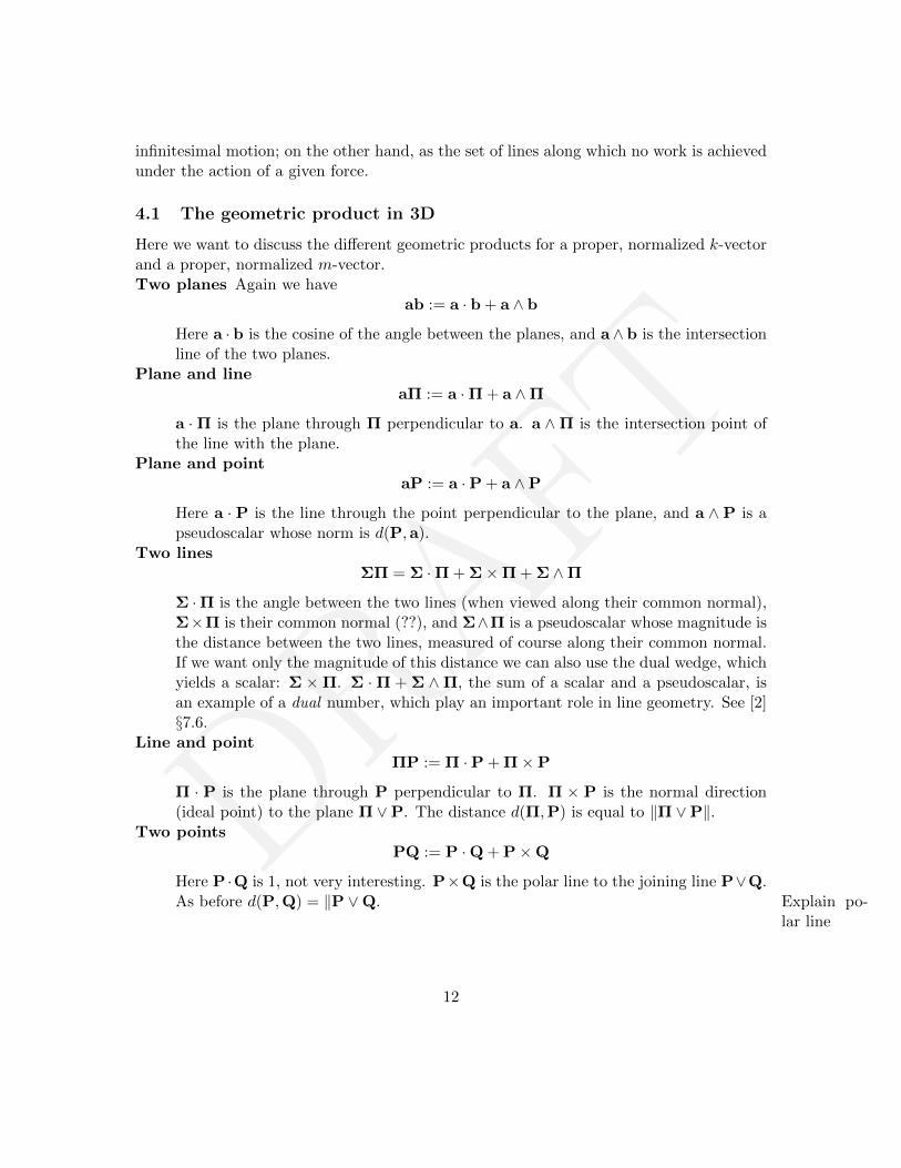
Here we want to discuss the different geometric products for a proper, normalized k-vectorand a proper, normalized m-vector.Two planes Again we have

ab := a · b + a ∧ b

Here a · b is the cosine of the angle between the planes, and a∧ b is the intersectionline of the two planes.

Plane and lineaΠ := a ·Π + a ∧Π

a ·Π is the plane through Π perpendicular to a. a ∧Π is the intersection point ofthe line with the plane.

Plane and pointaP := a ·P + a ∧P

Here a · P is the line through the point perpendicular to the plane, and a ∧ P is apseudoscalar whose norm is d(P,a).

Two linesΣΠ = Σ ·Π + Σ×Π + Σ ∧Π

Σ ·Π is the angle between the two lines (when viewed along their common normal),Σ×Π is their common normal (??), and Σ∧Π is a pseudoscalar whose magnitude isthe distance between the two lines, measured of course along their common normal.If we want only the magnitude of this distance we can also use the dual wedge, whichyields a scalar: Σ ×Π. Σ ·Π + Σ ∧Π, the sum of a scalar and a pseudoscalar, isan example of a dual number, which play an important role in line geometry. See [2]§7.6.

Line and pointΠP := Π ·P + Π×P

Π · P is the plane through P perpendicular to Π. Π × P is the normal direction(ideal point) to the plane Π ∨P. The distance d(Π,P) is equal to ‖Π ∨P‖.

Two pointsPQ := P ·Q + P×Q

Here P ·Q is 1, not very interesting. P×Q is the polar line to the joining line P∨Q.As before d(P,Q) = ‖P ∨Q. Explain po-

lar line

12

DRAFT

P

Π

P

Π

Π.P

P

Π

Π.P

(Π.P)ΛΠ

P

Π

Π.P ((Π.P)ΛΠ)VP

(Π.P)ΛΠ

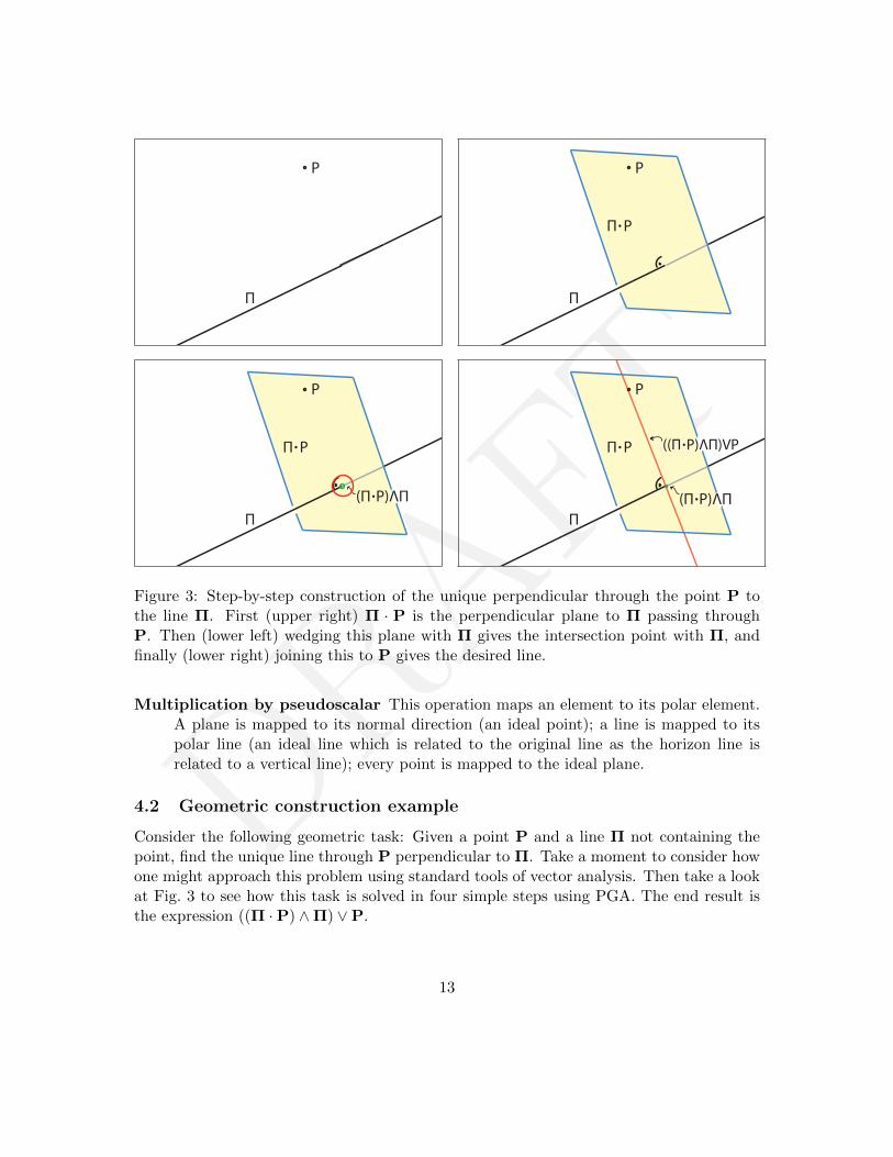
Figure 3: Step-by-step construction of the unique perpendicular through the point P tothe line Π. First (upper right) Π · P is the perpendicular plane to Π passing throughP. Then (lower left) wedging this plane with Π gives the intersection point with Π, andfinally (lower right) joining this to P gives the desired line.

Multiplication by pseudoscalar This operation maps an element to its polar element.A plane is mapped to its normal direction (an ideal point); a line is mapped to itspolar line (an ideal line which is related to the original line as the horizon line isrelated to a vertical line); every point is mapped to the ideal plane.

4.2 Geometric construction example

Consider the following geometric task: Given a point P and a line Π not containing thepoint, find the unique line through P perpendicular to Π. Take a moment to consider howone might approach this problem using standard tools of vector analysis. Then take a lookat Fig. 3 to see how this task is solved in four simple steps using PGA. The end result isthe expression ((Π ·P) ∧Π) ∨P.

13

DRAFT

4.3 A table of useful geometric formulae in 3D PGA

Table 1 is based on the above discussions of the geometric product and of sandwich oper-ations, and demonstrates the power of PGA to represent 3D geometric calculations com-pactly and completely. Many of the examples have been taken from the collection of graph-ics gems [1]; we don’t include the original solutions in the table due to space limitations.

4.4 Isometries in 3D, or “Where do (dual) quaternions come from?”

The same principles developed above in the discussion of reflections, rotations, and trans-lations in 2D can be applied without change in 3D. Sandwich operators with 1-vectorsproduce reflections in the corresponding planes; applying two such reflections one after theother – in non-parallel planes – produces a rotation around the intersection line of the twoplanes of twice the angle between the two planes. When the two planes are parallel, oneobtains translations in the normal direction to the planes of twice the distance between thetwo planes. But that’s not all. If I compose a rotation around a line with a translation inthe direction of the line I obtain a new kind of isometry, a so-called screw motion, which, incontrast to the isometries discussed previously, has a single proper fixed line but no properfixed points. It is the generic direct isometry of euclidean space.

4.4.1 The quaternions

Restrict attention to the subspace of bivectors spanned by {e12, e31, e23}. These are all lineswhich pass through the origin E0. They give rise by exponentiation to rotations aroundthe three coordinate axes. Then the elements {1, e12, e31, e23} generate a 4-dimensionalsubalgebra of P(R∗3,0,1) isomorphic to the quaternions. The subset of normed elements(such that gg = 1 represent the rotor group fixing the origin, and are isomorphic to theunit quaternions.

Exercise. Verify the claims in the previous paragraph.

4.4.2 The dual quaternions

Consider first the bivectors {e01, e02, e03} which represent the three ideal lines aligned withthe coordinate planes. They span the subspace consisting of ideal lines. Exponentiatingthese bivectors produces translators. Then the elements {1, e01, e02, e03} generate a 4-dimensional subalgebra of P(R∗3,0,1) not isomorphic to the quaternions since all bivectors

have square 0. The subalgebra has the (commutative) group structure of R4; the translatorgroup has the group structure of R3 (normalized here means scalar part is 1).

A general screw motion – as described above – can be written as a rotation around aproper line Σ followed by a translation in the direction of Σ. The latter translation is givenby a translator of the form 1 + dΣI (Exercise). That is, a translation in the direction of

14

DRAFT

Operation PGA

Line from two points P ∨Q

Line from two planes a ∧ b

Point from three planes a ∧ b ∧ c

Plane from three points P ∨Q ∨R

Oriented distance point to plane ‖a ∨P‖Distance of two points ‖P ∨Q‖Angle of two planes cos−1(a · b)

Line through point perpendicular to plane P · aOrthogonal projection point to plane (P · a)a

Plane through point parallel to plane (P · a)P

Intersection of line and plane Π ∧ a

Plane through point perpendicular to line Π ·POrthogonal projection point to line (P ·Π)Π

Line through point parallel to line (P ·Π)P

Line through point perpendicular to line ((P ·Π)P) ∨P

Oriented distance of two lines Π ∨Σ

Angle of two lines Π ·ΣReflection in plane aXa

Rotation around line through angle 2α RXR (R := eαΠ)

Translation by the vector 2v TXT (T := eI(E0∨v))

Screw motion along axis with pitch α SXS (S := e(1+αI)Π)

Table 1: A sample of geometric constructions in P(R∗3,0,1).

15

DRAFT

a given line is a “rotation” around the polar line ΣI of Σ. For example, suppose Σ = e12is the z-axis. Then ΣI = e03 is the ideal line of the z = 0 plane, the “horizon” line. A“rotation” around this ideal line moves all points parallel to the z-direction, in the directionof the original line Σ. Thus (leaving some steps to the reader) any screw motion can bewritten as et(1+βI)Σ for some t > 0, some proper line Σ – the axis of the screw motion– and real β. β is a parameter called the pitch of the screw motion and describes thesteepness of the spiraling. β = 0 is a rotation, β =∞ is a translation (actually to model atranslation we use etΣI).

The spin group which arises in this general setting is a double covering of the six-dimensional euclidean group. It sits in the even subalgebra P(R∗+3,0,1). It is isomorphic tothe dual quaternions under the mapping which sends:

1→ 1

e12 → i

e23 → j

e31 → k

I→ ε

This implies in particular that

e01 = e23I→ εk

e02 = e31I→ εj

e03 = e12I→ εi

That is, the mysterious unit ε in the dual numbers is mirrored in the geometric algebrasetting by the pseudoscalar I which encodes the metric of euclidean space. In this iso-morphism, the dual numbers are important because they are the possible values of Σ2.Operating with dual numbers allows one to write the exponentials above in terms of theexponentials of simple bivectors (lines) whose square are guaranteed to −1 or 0, ratherthan line complexes. This leads to a secure convergence theory for the exponential powerseries.

Exercise. Interpret your favorite features of the dual quaternions in terms of their em-bedding in the geometric algebra P(R∗3,0,1).

Other metrics. One of the nice features of this approach is that the whole machineryworks also in non-euclidean settings. If instead of e20 = 0 we choose e20 = 1 or e20 = −1,one obtains elliptic resp. hyperbolic space and can work with the same basic elements inexactly analogous ways to do geometry in these spaces also. See [2] for details.

16

DRAFT

5 Conclusion

[Remains to be written]Those interested in a full account, please consult [3], [4], or [2].

References

[1] Andrew S. Glassner. Graphics Gems. Academic Press, 1990.

[2] Charles Gunn. Geometry, Kinematics, and Rigid Body Mechanics in Cayley-KleinGeometries. PhD thesis, Technical University Berlin, 2011. http://opus.kobv.de/tuberlin/volltexte/2011/3322.

[3] Charles Gunn. On the homogeneous model of euclidean geometry. In Leo Dorstand Joan Lasenby, editors, A Guide to Geometric Algebra in Practice, chapter 15,pages 297–327. Springer, 2011. http://page.math.tu-berlin.de/˜gunn/Documents/Papers/GAInPracticeCh15Gunn.pdf.

[4] Charles Gunn. On the homogeneous model of euclidean geometry: Extended version.http://arxiv.org/abs/1101.4542, 2011.

[5] Felix Klein. Uber Liniengeometrie und metrische Geometrie. Mathematische Annalen,5:106–126, 1872.

[6] J. Michael McCarthy. An Introduction to Theoretical Kinematics. MIT Press, Cam-bridge, MA, 1990.

[7] Eduard Study. Geometrie der Dynamen. Tuebner, Leibzig, 1903.

17