. CSPBankability Project Report Draft for an Appendix C – Solar Field Modeling to the SolarPACES Guideline for Bankable STE Yield Assessment Document prepared by the project CSPBankability funded by the German Federal Ministry Economic Affairs and Energy under contract No. 0325293.

Welcome message from author
This document is posted to help you gain knowledge. Please leave a comment to let me know what you think about it! Share it to your friends and learn new things together.
Transcript

.
CSPBankability Project Report
Draft for an
Appendix C – Solar Field Modeling
to the SolarPACES Guideline for
Bankable STE Yield Assessment
Document prepared by the project CSPBankability funded by the German Federal Ministry Economic Affairs and Energy under contract No. 0325293.

CSPBankability Project Report Draft for an Appendix C – Solar Field Modeling to the SolarPACES Guideline for Bankable STE Yield Assessment
Page: 2
Document properties
Title CSPBankability Project Report: Draft for an Appendix C – Solar Field Modeling to the SolarPACES Guideline for Bankable STE Yield Assessment
Editor Tobias Hirsch (DLR)
Author Jürgen Dersch, Stefano Giuliano (DLR)
Contributing authors
Enver Yildiz (Fichtner) Camille Bachelier (Frenell) Simon Lude Olaf Goebel (University of Applied Science Hamm-Lippstadt) Norbert Schmidt (DNV-GL) Michael Puppe (DLR) Christoph Rau (IATech)
Date January 9, 2017

CSPBankability Project Report Draft for an Appendix C – Solar Field Modeling to the SolarPACES Guideline for Bankable STE Yield Assessment
Page: 3
Index of contents
Document properties ..................................................................................................................... 2
C. Modelling of “Solar field SF” .................................................................................................... 4 C.1. General modeling approach .................................................................................................... 4 C.1.1. Generic modeling approach ................................................................................................... 4 C.1.2. Definition of the relevant aperture area ............................................................................... 6 C.1.3. Interface and result variables for the solar field sub-system ................................................ 6 C.2. Line focusing solar fields .......................................................................................................... 8 C.2.1. Parabolic trough field with oil ................................................................................................ 8
C.2.1.1. Specific modeling approach for this technology ........................................................... 9 C.2.1.2. Optical losses ............................................................................................................................ 15 C.2.1.3. Thermal losses ......................................................................................................................... 28 C.2.1.4. Pressure loss ............................................................................................................................. 39 C.2.1.5. Auxiliary electrical consumption...................................................................................... 40 C.2.1.6. Losses caused by operational limits................................................................................ 41 C.2.1.7. Transient effects ...................................................................................................................... 42 C.2.1.8. Night operation and freeze protection ........................................................................... 45 C.2.1.9. Interface variables .................................................................................................................. 47 C.2.1.10. Plausibility checks .................................................................................................................. 48
C.2.2. Parabolic trough field with two-phase heat transfer fluid (place holder) ........................... 49 C.2.3. Linear Fresnel field with single phase heat transfer fluid (place holder) ............................ 49 C.2.4. Linear Fresnel field with two-phase heat transfer fluid (place holder) ............................... 49 C.3. Solar towers ........................................................................................................................... 49 C.4. Symbols .................................................................................................................................. 50 C.4.1. Symbols used in chapter C.2 ................................................................................................ 50 C.5. References ............................................................................................................................. 54

CSPBankability Project Report Draft for an Appendix C – Solar Field Modeling to the SolarPACES Guideline for Bankable STE Yield Assessment
Page: 4
C. Modelling of “Solar field SF”
The solar field collects energy delivered by sun beams, converts it into sensible and/or latent heat of a fluid, and transports the heat via this fluid to the power block and/or to the thermal storage. Depending on individual CSP technologies solar field look different which in turn leads to specific modelling approaches. This appendix starts with a general approach and then turns to the specific ones with models for each physical effect with significant impact on the annual yield. In the current context “significant” means that neglecting the individual effect would change the annual electrical yield by approximately 1 % or more.
C.1. General modeling approach
Although the solar field technologies differ some fundamentals are very similar and allow to define generic approaches applicable to all of them. This section introduces some general aspects that are used by the technology-specific chapters that follow. These are:
• An generic equation for describing steady-state performance • The definition of the aperture area • Interface and monitoring variables.
C.1.1. Generic modeling approach
The general quasi dynamic equation for the thermal power delivered by the solar field of CSP systems may be written as: �̇�𝑄SF = �̇�𝑄avail −��̇�𝑄loss + ��̇�𝑄gain − �̇�𝑄𝑡𝑡𝑡𝑡𝑡𝑡𝑡𝑡𝑡𝑡 (C.1)
It consists of the available radiant solar power reduced by thermal losses and increased by heat gains from other sources (e.g. the power of solar field pumps but also from trace heating if applicable) and a transient correction term. According to the general energy chain, the available radiant solar power reduced by all optical losses is leading to the absorbed thermal power. �̇�𝑄abs = 𝜂𝜂𝑜𝑜𝑜𝑜𝑡𝑡 �̇�𝑄𝑡𝑡𝑎𝑎𝑡𝑡𝑎𝑎𝑎𝑎 (C.2)
The absorbed thermal power for many CSP systems consists of 2 parts: the irradiance collected by the reflectors and redirected to the receiver and the irradiance which hits the receiver directly. The latter one is typically much smaller than the first one since the reflective area is much larger than the receiver area.

CSPBankability Project Report Draft for an Appendix C – Solar Field Modeling to the SolarPACES Guideline for Bankable STE Yield Assessment
Page: 5
Following formula allows for determination of the absorbed thermal power: �̇�𝑄abs = 𝜂𝜂phi 𝜂𝜂shad 𝜂𝜂refl,0 𝜂𝜂reflclean 𝜂𝜂block 𝜂𝜂atten
𝜂𝜂inter 𝜂𝜂recclean 𝜂𝜂trans 𝜂𝜂abs 𝜂𝜂avail 𝑓𝑓focA 𝐴𝐴nom* 𝐺𝐺bn+ 𝐴𝐴rec �𝜂𝜂phi,rec𝐺𝐺bn + 𝐺𝐺d� 𝜂𝜂recclean 𝜂𝜂trans 𝜂𝜂abs
(C.3)
With: �̇�𝑄abs Absorbed thermal power in kW 𝜂𝜂phi Incidence angle efficiency including all losses caused by non-perpendicular sun rays into the aperture plane, dimensionless 𝜂𝜂shad Shading efficiency, dimensionless 𝜂𝜂refl,0 Clean reflector efficiency, dimensionless 𝜂𝜂reflclean Reflector cleanliness factor, dimensionless 𝜂𝜂block Blocking efficiency, dimensionless 𝜂𝜂atten Atmospheric attenuation efficiency, dimensionless 𝜂𝜂inter Intercept factor, dimensionless 𝜂𝜂recclean Receiver cleanliness factor, dimensionless 𝜂𝜂trans Transmission through receiver glass cover (if any), dimensionless 𝜂𝜂abs Receiver absorptance dimensionless 𝜂𝜂avail Solar field availability, dimensionless 𝑓𝑓focA Focusing factor, fraction of the actual aperture area in operation over the
total nominal aperture area, or fraction of the actual intercept efficiency over the nominal intercept efficiency
𝐴𝐴nom∗ Nominal aperture area without receiver area in m² 𝐴𝐴rec Receiver area in m² 𝐺𝐺bn Direct normal solar irradiance in W/m² 𝐺𝐺d Diffuse irradiance in W/m² The focusing factor 𝑓𝑓focA represents the fraction of the solar field aperture area actually in operation or the actual intercept efficiency over the nominal intercept efficiency, depending on the applied control strategy. During certain time periods the solar field must be partially defocused because the power block runs at maximal load and the thermal storage is fully charged. In order to prevent overheating some of the installed mirrors are turned in out of focus to adapt the actual solar field output to the desired output. For parabolic trough plants another control strategy is often used: instead of turning whole collectors or loops in a position where they do not collect any solar irradiance, they are just turned out of the ideal tracking position by a small angle in a way that a certain fraction of the reflected sun beams are not hitting the absorber tube. This control strategy enables a smoother adaption of the solar field output to the requirements than the one mentioned before. In terms of Eq. (C.3) this second control strategy means that the intercept efficiency of the system is reduced.
CSPBankability Project Report Draft for an Appendix C – Solar Field Modeling to the SolarPACES Guideline for Bankable STE Yield Assessment
Page: 6
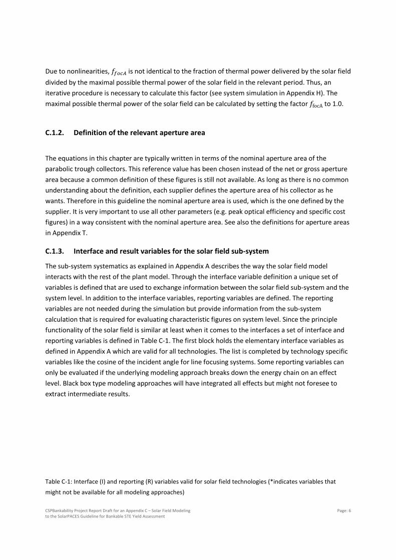
Due to nonlinearities, 𝑓𝑓𝑓𝑓𝑜𝑜𝑓𝑓𝑓𝑓 is not identical to the fraction of thermal power delivered by the solar field divided by the maximal possible thermal power of the solar field in the relevant period. Thus, an iterative procedure is necessary to calculate this factor (see system simulation in Appendix H). The maximal possible thermal power of the solar field can be calculated by setting the factor 𝑓𝑓focA to 1.0.
C.1.2. Definition of the relevant aperture area
The equations in this chapter are typically written in terms of the nominal aperture area of the parabolic trough collectors. This reference value has been chosen instead of the net or gross aperture area because a common definition of these figures is still not available. As long as there is no common understanding about the definition, each supplier defines the aperture area of his collector as he wants. Therefore in this guideline the nominal aperture area is used, which is the one defined by the supplier. It is very important to use all other parameters (e.g. peak optical efficiency and specific cost figures) in a way consistent with the nominal aperture area. See also the definitions for aperture areas in Appendix T.
C.1.3. Interface and result variables for the solar field sub-system
The sub-system systematics as explained in Appendix A describes the way the solar field model interacts with the rest of the plant model. Through the interface variable definition a unique set of variables is defined that are used to exchange information between the solar field sub-system and the system level. In addition to the interface variables, reporting variables are defined. The reporting variables are not needed during the simulation but provide information from the sub-system calculation that is required for evaluating characteristic figures on system level. Since the principle functionality of the solar field is similar at least when it comes to the interfaces a set of interface and reporting variables is defined in Table C-1. The first block holds the elementary interface variables as defined in Appendix A which are valid for all technologies. The list is completed by technology specific variables like the cosine of the incident angle for line focusing systems. Some reporting variables can only be evaluated if the underlying modeling approach breaks down the energy chain on an effect level. Black box type modeling approaches will have integrated all effects but might not foresee to extract intermediate results.
Table C-1: Interface (I) and reporting (R) variables valid for solar field technologies (*indicates variables that
might not be available for all modeling approaches)

CSPBankability Project Report Draft for an Appendix C – Solar Field Modeling to the SolarPACES Guideline for Bankable STE Yield Assessment
Page: 7
Type Name Symbol Comment
I Inlet temperature 𝑻𝑻inSF
I Outlet temperature 𝑻𝑻outSF
I Inlet pressure 𝒑𝒑inSF
I Outlet pressure 𝒑𝒑outSF
I mass flow �̇�𝒎SF
I Ambient temperature Tamb
I Direct normal irradiance Gbn
I Wind direction/speed 𝒗𝒗𝐰𝐰𝐰𝐰𝐰𝐰𝐰𝐰,
𝜸𝜸wind
I Auxiliary electrical demand 𝑷𝑷auxSF
I Acceptable minimum/maximum mass
flow
�̇�𝒎min/maxSF
I Set point outlet temperature 𝑻𝑻out,setSF
I Set point mass flow �̇�𝒎setSF
R Solar field thermal power �̇�𝑸SF
R Available radiant solar power �̇�𝑸avail
R Absorbed power �̇�𝑸abs
R Percentage of field operational* 𝒇𝒇foc,A
R Maximum load defocussing power* �̇�𝑸defoc,max
R Minimum load defocussing power* �̇�𝑸defoc,min
R Receiver heat loss power* �̇�𝑸loss,rec
R Solar field piping thermal loss power* �̇�𝑸loss,pipe
R Header piping thermal loss power* �̇�𝑸loss,head
R HTF equipment thermal loss power* �̇�𝑸loss,equ
CSPBankability Project Report Draft for an Appendix C – Solar Field Modeling to the SolarPACES Guideline for Bankable STE Yield Assessment
Page: 8
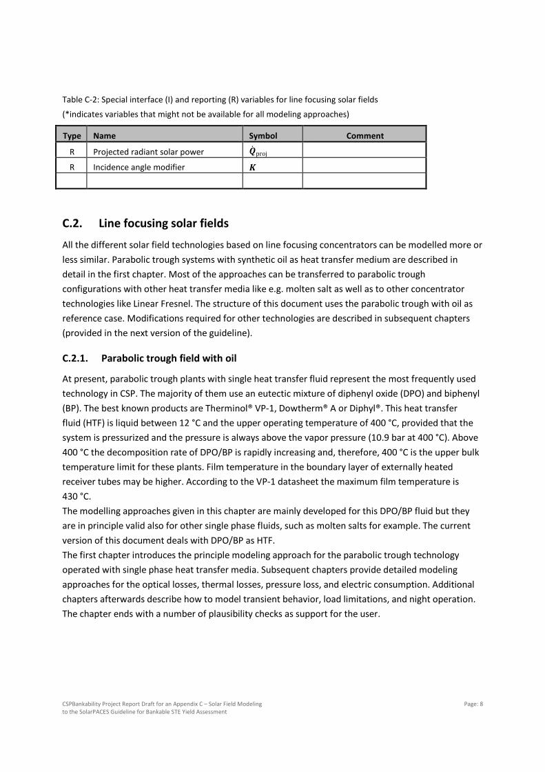
Table C-2: Special interface (I) and reporting (R) variables for line focusing solar fields
(*indicates variables that might not be available for all modeling approaches)
Type Name Symbol Comment
R Projected radiant solar power �̇�𝑸proj
R Incidence angle modifier 𝑲𝑲
C.2. Line focusing solar fields
All the different solar field technologies based on line focusing concentrators can be modelled more or less similar. Parabolic trough systems with synthetic oil as heat transfer medium are described in detail in the first chapter. Most of the approaches can be transferred to parabolic trough configurations with other heat transfer media like e.g. molten salt as well as to other concentrator technologies like Linear Fresnel. The structure of this document uses the parabolic trough with oil as reference case. Modifications required for other technologies are described in subsequent chapters (provided in the next version of the guideline).
C.2.1. Parabolic trough field with oil
At present, parabolic trough plants with single heat transfer fluid represent the most frequently used technology in CSP. The majority of them use an eutectic mixture of diphenyl oxide (DPO) and biphenyl (BP). The best known products are Therminol® VP-1, Dowtherm® A or Diphyl®. This heat transfer fluid (HTF) is liquid between 12 °C and the upper operating temperature of 400 °C, provided that the system is pressurized and the pressure is always above the vapor pressure (10.9 bar at 400 °C). Above 400 °C the decomposition rate of DPO/BP is rapidly increasing and, therefore, 400 °C is the upper bulk temperature limit for these plants. Film temperature in the boundary layer of externally heated receiver tubes may be higher. According to the VP-1 datasheet the maximum film temperature is 430 °C. The modelling approaches given in this chapter are mainly developed for this DPO/BP fluid but they are in principle valid also for other single phase fluids, such as molten salts for example. The current version of this document deals with DPO/BP as HTF. The first chapter introduces the principle modeling approach for the parabolic trough technology operated with single phase heat transfer media. Subsequent chapters provide detailed modeling approaches for the optical losses, thermal losses, pressure loss, and electric consumption. Additional chapters afterwards describe how to model transient behavior, load limitations, and night operation. The chapter ends with a number of plausibility checks as support for the user.
CSPBankability Project Report Draft for an Appendix C – Solar Field Modeling to the SolarPACES Guideline for Bankable STE Yield Assessment
Page: 9
C.2.1.1. Specific modeling approach for this technology
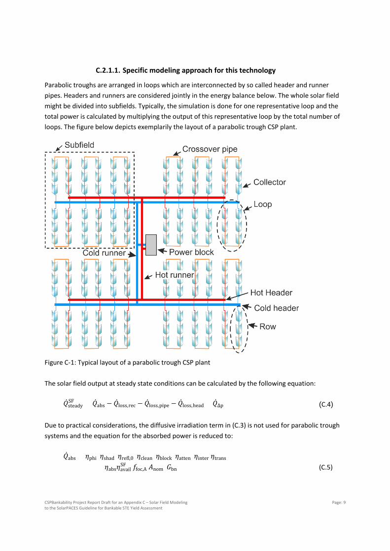
Parabolic troughs are arranged in loops which are interconnected by so called header and runner pipes. Headers and runners are considered jointly in the energy balance below. The whole solar field might be divided into subfields. Typically, the simulation is done for one representative loop and the total power is calculated by multiplying the output of this representative loop by the total number of loops. The figure below depicts exemplarily the layout of a parabolic trough CSP plant.
Figure C-1: Typical layout of a parabolic trough CSP plant The solar field output at steady state conditions can be calculated by the following equation: �̇�𝑄steady
SF = �̇�𝑄abs − �̇�𝑄loss,rec − �̇�𝑄loss,pipe − �̇�𝑄loss,head + �̇�𝑄∆p (C.4) Due to practical considerations, the diffusive irradiation term in (C.3) is not used for parabolic trough systems and the equation for the absorbed power is reduced to: �̇�𝑄abs = 𝜂𝜂phi 𝜂𝜂shad 𝜂𝜂refl,0 𝜂𝜂clean 𝜂𝜂block 𝜂𝜂atten 𝜂𝜂inter 𝜂𝜂trans
𝜂𝜂abs𝜂𝜂availSF 𝑓𝑓foc,A 𝐴𝐴nom 𝐺𝐺bn
(C.5)

CSPBankability Project Report Draft for an Appendix C – Solar Field Modeling to the SolarPACES Guideline for Bankable STE Yield Assessment
Page: 10
Nevertheless, the irradiance absorbed directly by the receiver is not neglected in (C.5) since the nominal aperture area in this equation is typically defined in a manner that the receiver area is included, in contrast to 𝐴𝐴nom∗ used in Eq. (C.3). This might be considered as a slightly conservative approach since the diffuse irradiance onto the receiver is neglected and the direct irradiance on it is reduced by the reflectivity of the mirrors although the irradiance is not redirected by the mirrors. The cleanliness is considered by a single effective value. Furthermore, several effects from Eq. (C.3) are merged into the peak optical efficiency as shown in Eq. (C.6). This peak optical efficiency is defined for a single collector, a complete device of around 100 m in length or more for usual commercial industrial scale collectors, which can be tracked as one unit. 𝜂𝜂opt,0 = 𝜂𝜂refl,0 𝜂𝜂block 𝜂𝜂atten 𝜂𝜂inter 𝜂𝜂trans 𝜂𝜂abs (C.6) The optical efficiency is measured by manufacturers or laboratories and given on the collector data sheets. For the utilization of the relevant value in terms of a model, it is important that optical efficiency and corresponding nominal aperture area are specified together since the value of the optical efficiency depends on the actual definition of aperture area. The same statement is valid for specific costs based on the aperture area. The following table shows 2 different aperture areas for Eurotrough SKAL-ET collectors and the corresponding optical efficiencies. The nominal aperture area of 817.5 m² and corresponding optical efficiency of 78 % have been published by [Herrmann 2004]. If the gross aperture area calculated from the collector outer dimensions is used in the equations for the calculation of the solar field output instead of the nominal aperture, the optical efficiency value must be reduced by 3.6 % points in order to yield the correct absorbed power. The example shows that the aperture area definition and the corresponding performance data need to be carefully checked for consistence before they are used for the yield calculation.
Table C-3: Two coupled pairs of aperture area and optical efficiency for the Eurotrough collector
Parameter value unit Nominal aperture area 817.5 m² Nominal optical efficiency 78 % Collector length 148.5 m Aperture width 5.77 m Gross aperture area 856.8 m² Gross optical efficiency 74.4 % The optical efficiency is only valid for a certain combination of reflector and receiver and must be determined for each collector. Design modifications of the collector or utilization of other receiver types will lead to other optical efficiency of the system.

CSPBankability Project Report Draft for an Appendix C – Solar Field Modeling to the SolarPACES Guideline for Bankable STE Yield Assessment
Page: 11
Table C-4: Reference value for the optical efficiency of the Eurotrough collector and typical range for the optical
efficiency of parabolic trough collectors
Reference value Default value
Range Uncertainty unit
Nominal optical efficiency 0.78 0.65 … 0.82 t.b.d. - Nominal aperture area 817.5 n.a. n.a. m² The efficiency term used for losses caused by non-perpendicular incoming sun rays into the aperture plane is expressed by cosine losses, incidence angle modifier K, and end losses. 𝜂𝜂phi = cos(𝜃𝜃i) ∙ 𝐾𝐾(𝜃𝜃i) ∙ 𝜂𝜂endloss (C.7) Typically, the solar field is made of many identical collectors, thus the total absorbed thermal power of the solar field, a single loop or a single collector may be calculated by: �̇�𝑄abs = 𝑐𝑐𝑐𝑐𝑐𝑐(𝜃𝜃i) 𝐾𝐾(𝜃𝜃i) 𝜂𝜂endloss 𝜂𝜂opt,0 𝜂𝜂shad 𝜂𝜂clean 𝜂𝜂avail 𝑓𝑓focA 𝐴𝐴nom 𝐺𝐺bn (C.8) Or, in terms of the projected direct irradiance: �̇�𝑄abs = 𝐾𝐾(𝜃𝜃i) 𝜂𝜂endloss 𝜂𝜂opt,0 𝜂𝜂shad 𝜂𝜂clean 𝜂𝜂avail 𝑓𝑓focA 𝐴𝐴nom 𝐺𝐺pr (C.9) With the appropriate total area Anom of the whole solar field, of one loop or of one collector, respectively. The proposal in this handbook is to calculate the absorbed heat for a single representative loop since many heat loss effects can easily be calculated for a single loop. Should the solar field consist of different collector types or different loop arrangements, these subfields may be calculated separately and results for the total field may be generated by summing up the individual results. For parabolic trough solar fields, defocusing can be done for whole loops or by defocusing some or all collectors in each loop by a small fraction and reducing the intercept efficiency by this measure. The second approach allows for smoother operation and is considered in this model. Therefore, the factor 𝑓𝑓focA is valid for the whole solar field as well as for single loops. Incidence angle for parabolic troughs The incidence angle of the sun rays onto the aperture is of particular importance for parabolic troughs and other single axis tracking CSP systems.
CSPBankability Project Report Draft for an Appendix C – Solar Field Modeling to the SolarPACES Guideline for Bankable STE Yield Assessment
Page: 12
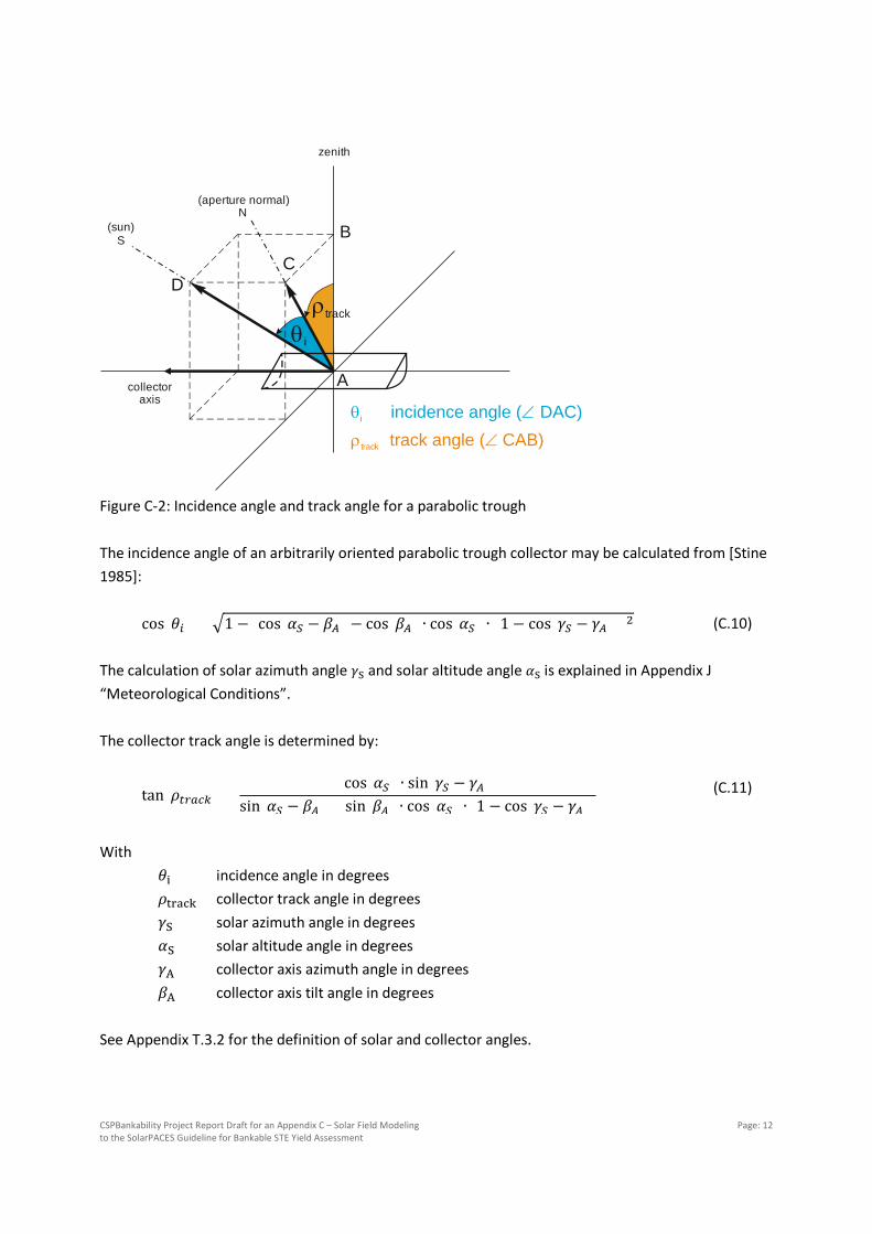
Figure C-2: Incidence angle and track angle for a parabolic trough The incidence angle of an arbitrarily oriented parabolic trough collector may be calculated from [Stine 1985]: cos(𝜃𝜃𝑎𝑎) = �1 − [cos(𝛼𝛼𝑆𝑆 − 𝛽𝛽𝑓𝑓) − cos(𝛽𝛽𝑓𝑓) ∙ cos(𝛼𝛼𝑆𝑆) ∙ (1 − cos(𝛾𝛾𝑆𝑆 − 𝛾𝛾𝑓𝑓))]2 (C.10) The calculation of solar azimuth angle 𝛾𝛾S and solar altitude angle 𝛼𝛼S is explained in Appendix J “Meteorological Conditions”. The collector track angle is determined by: tan(𝜌𝜌𝑡𝑡𝑡𝑡𝑡𝑡𝑓𝑓𝑡𝑡) =
cos(𝛼𝛼𝑆𝑆) ∙ sin(𝛾𝛾𝑆𝑆 − 𝛾𝛾𝑓𝑓)sin(𝛼𝛼𝑆𝑆 − 𝛽𝛽𝑓𝑓) + sin(𝛽𝛽𝑓𝑓) ∙ cos(𝛼𝛼𝑆𝑆) ∙ [1 − cos(𝛾𝛾𝑆𝑆 − 𝛾𝛾𝑓𝑓)] (C.11)
With 𝜃𝜃i incidence angle in degrees 𝜌𝜌track collector track angle in degrees 𝛾𝛾S solar azimuth angle in degrees 𝛼𝛼S solar altitude angle in degrees 𝛾𝛾A collector axis azimuth angle in degrees 𝛽𝛽A collector axis tilt angle in degrees See Appendix T.3.2 for the definition of solar and collector angles.
(aperture normal) N
(sun)S
zenith
collectoraxis
A
B
CD
ρtrack
θi
ρtrack track angle ( CAB)∠iθ incidence angle ( DAC)∠

CSPBankability Project Report Draft for an Appendix C – Solar Field Modeling to the SolarPACES Guideline for Bankable STE Yield Assessment
Page: 13
Users should take particular care of the time of reference used in the annual performance calculation and in the meteorological dataset. Meteorological datasets derived from satellite data often use coordinated universal time (UTC) since satellite images typically cover several time zones. Annual performance models in contrast often use local time at site since this allows for direct comparison of the generated electricity with demand profiles or time dependent tariffs. The situation gets even more complicated when daylight saving time is observed during summer months at the specific site. In this case, a meteorological dataset based on daylight savings time has missing or surplus values for those hours when the local time is shifted to daylight saving time or vice versa. The recommendation is to stay with UTC or local (winter time) for the technical simulations and consider the time shift in the load or tariff matrix. Furthermore, it is important to check the definition of the time stamp used in the meteorological data file. Time stamp means that the meteorological data file and also the model output will use a time indication which actually stands for a time period. Therefore, at least three interpretations are possible for the relation between time stamp and associated period: the time stamp represents the preceding period, the following period or the center of the period. In this handbook, we assume that a time stamp like 12:00 in a file with hourly resolution means that the data represents the mean values of DNI, ambient temperature, ambient humidity, etc. in the preceding time step. Therefore, the corresponding mean sun position is that of 11:30! This is valid for most hours of the day except for the time periods of sunrise and sunset. The sun position in the middle of those hours might be below horizon and therefore not representative for the yield calculation. Instead, the sun position for these hours should be calculated for the center of the time interval between sunrise and the next time stamp in the morning and between the previous time stamp and sunset in the evening. For datasets with higher temporal resolution than one hour this rule can be applied accordingly. Example for the correction of DNI and sun position for hourly time steps In case of large time steps like 1 hour for the simulation it might be necessary to pay particular attention to the time steps of sunrise and sunset. Sun position and mean DNI values should be checked and corrected if necessary. Figure C-3 shows an example for the correction of DNI and sun position in case of large time steps like 1 hour. Sunrise is just after 6:30 and the 10 minutes dataset shows 1, 99 and 295 W/m² for the first three time steps after sunrise. Mean DNI using hourly resolution would result in 66 W/m² for this first hour. For the simulation it makes a difference whether the mean values (averaged over one hour) of DNI and sun position are used or corrected values for DNI and sun position that take into account the sunrise event. Let us assume that only the information of the blue columns (mean hourly values) in Figure C-3 is available, together with the time of sunrise. The 10 min data in this figure are just shown for demonstration purposes. First, the corrected solar position to be used for the performance calculation needs to be calculated based on the time of sunrise for 6:45. In the next step, the hourly averaged DNI of 66 W/m2 needs to be corrected for the time interval after sunrise (66 W/m²*60 min/29 min = 137 W/m²). The difference between the original 66 W/m2 and the corrected 137 W/m2

CSPBankability Project Report Draft for an Appendix C – Solar Field Modeling to the SolarPACES Guideline for Bankable STE Yield Assessment
Page: 14
is significant. Prior to the application of this kind of correction, it must be checked whether it was not already done during the compilation of the meteorological dataset (see Appendix J) in order to avoid a double correction!
Figure C-3: Mean DNI for different temporal resolutions and solar altitude angle in early morning hours However, when 10 minutes are used as time step for the whole simulation, it will be sufficient to use always the sun position at the middle of the time interval together with the beam radiation from the meteorological data file. The error of this simplification is negligible. For low solar altitude angles (< 10°) row-to-row shading as well as high atmospheric attenuation reduce the usable direct irradiance. It is recommended to carry out a simulation also for those time steps and check whether a positive heat gain is possible or not. Operators in existing plants may use a certain threshold solar altitude angle instead of such a calculation. However, such threshold angle is difficult to determine in a common way. Thus, having the model available it will be easier to determine whether there is a net heat gain from the solar field or not. Impact of temporal resolutions on annual performance results The required temporal resolution for annual performance models is a matter of discussion since several years. This guideline recommends the utilization of 10 minutes time steps since high quality meteorological date is typically available with this resolution, modern computers are fast enough and the model formulation is simpler, particularly for those time steps with startup operation or when certain limits are reached (e.g. storage is totally charged or discharged). When hourly time steps are
0
5
10
15
20
25
0
100
200
300
400
500
600
700
800
900
Sola
r alti
tude
ang
le in
°
DN
I in
W/m
²
Time
hourly DNI
10 min DNI
solar altitude angle
CSPBankability Project Report Draft for an Appendix C – Solar Field Modeling to the SolarPACES Guideline for Bankable STE Yield Assessment
Page: 15
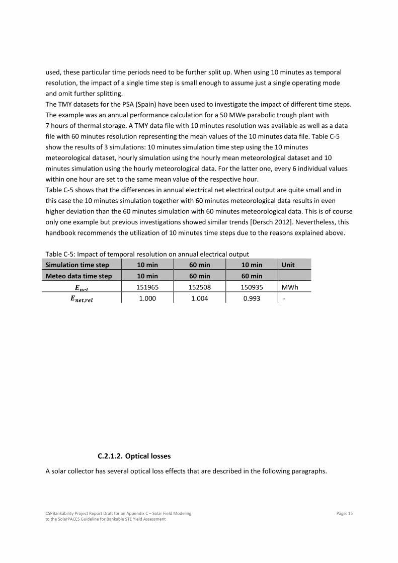
used, these particular time periods need to be further split up. When using 10 minutes as temporal resolution, the impact of a single time step is small enough to assume just a single operating mode and omit further splitting. The TMY datasets for the PSA (Spain) have been used to investigate the impact of different time steps. The example was an annual performance calculation for a 50 MWe parabolic trough plant with 7 hours of thermal storage. A TMY data file with 10 minutes resolution was available as well as a data file with 60 minutes resolution representing the mean values of the 10 minutes data file. Table C-5 show the results of 3 simulations: 10 minutes simulation time step using the 10 minutes meteorological dataset, hourly simulation using the hourly mean meteorological dataset and 10 minutes simulation using the hourly meteorological data. For the latter one, every 6 individual values within one hour are set to the same mean value of the respective hour. Table C-5 shows that the differences in annual electrical net electrical output are quite small and in this case the 10 minutes simulation together with 60 minutes meteorological data results in even higher deviation than the 60 minutes simulation with 60 minutes meteorological data. This is of course only one example but previous investigations showed similar trends [Dersch 2012]. Nevertheless, this handbook recommends the utilization of 10 minutes time steps due to the reasons explained above. Table C-5: Impact of temporal resolution on annual electrical output Simulation time step 10 min 60 min 10 min Unit Meteo data time step 10 min 60 min 60 min
𝑬𝑬𝒏𝒏𝒏𝒏𝒏𝒏 151965 152508 150935 MWh 𝑬𝑬𝒏𝒏𝒏𝒏𝒏𝒏,𝒓𝒓𝒏𝒏𝒓𝒓 1.000 1.004 0.993 -
C.2.1.2. Optical losses
A solar collector has several optical loss effects that are described in the following paragraphs.

CSPBankability Project Report Draft for an Appendix C – Solar Field Modeling to the SolarPACES Guideline for Bankable STE Yield Assessment
Page: 16
Figure C-4: Sankey diagram showing the energy chain from solar resource to heat delivered by the solar field Cosine losses When the collector aperture is not perpendicular to the sun rays, the projected aperture area is reduced. Parabolic trough collectors are tracked in a manner that sun beams are within the plane defined by the collector aperture normal and the collector axis. Since parabolic trough collectors are single axis tracking collectors there is a certain angle between sun vector and aperture normal vector for most sun positions (the incidence angle). Thus, the apparent aperture area as seen from the sun is reduced. The reduced aperture area depends on the cosine of the incidence angle which is the reason for calling these losses cosine losses. 𝜂𝜂cos = 𝑐𝑐𝑐𝑐𝑐𝑐(𝜃𝜃i) =
𝐺𝐺pr
𝐺𝐺bn (C.12)

CSPBankability Project Report Draft for an Appendix C – Solar Field Modeling to the SolarPACES Guideline for Bankable STE Yield Assessment
Page: 17
Figure C-5: Effective aperture reduction caused by non-perpendicular sun rays onto the aperture (cosine losses) Row-to row shading If there are no mountains or other huge structures close to the solar field, the major shading mechanism is the so called row-to-row shading caused by other parabolic troughs of the neighbor row in the solar field. Shading caused by nearby buildings or mountains etc. is considered in the next paragraph.
Figure C-6: Row-to-row shading in a parabolic trough solar field Row-to-row shading is a geometrical effect and can be calculated from:
θi
θi
sun beams
actual aperture aea
reduced aperture area
θi : incident angle
zenith
sun beams
wcol
drow
shaded
surface
ρ tr

CSPBankability Project Report Draft for an Appendix C – Solar Field Modeling to the SolarPACES Guideline for Bankable STE Yield Assessment
Page: 18
𝜂𝜂shad,row =𝑑𝑑𝑡𝑡𝑜𝑜𝑟𝑟 𝑐𝑐𝑐𝑐𝑐𝑐(𝜌𝜌𝑡𝑡𝑡𝑡)
𝑤𝑤𝑓𝑓𝑜𝑜𝑎𝑎 for 0 ≤
𝑑𝑑𝑡𝑡𝑜𝑜𝑟𝑟 𝑐𝑐𝑐𝑐𝑐𝑐(𝜌𝜌𝑡𝑡𝑡𝑡)𝑤𝑤𝑓𝑓𝑜𝑜𝑎𝑎
≤ 1
𝜂𝜂shad,row = 0 for 𝑑𝑑𝑡𝑡𝑜𝑜𝑟𝑟 𝑐𝑐𝑐𝑐𝑐𝑐(𝜌𝜌𝑡𝑡𝑡𝑡)
𝑤𝑤𝑓𝑓𝑜𝑜𝑎𝑎 < 0
𝜂𝜂shad,row = 1 for 𝑑𝑑𝑡𝑡𝑜𝑜𝑟𝑟 𝑐𝑐𝑐𝑐𝑐𝑐(𝜌𝜌𝑡𝑡𝑡𝑡)
𝑤𝑤𝑓𝑓𝑜𝑜𝑎𝑎 > 1
(C.13)
With: 𝑤𝑤col collector aperture width in m 𝑑𝑑row row-to-row distance in m Row-to-row shading has only a significant impact for low solar altitude angles. Most of the existing large parabolic trough solar fields use a row distance of about 3 aperture widths and south-north oriented collector axes. For these configurations the annual row-to-row shading losses are typically lower than 1 % compared to the annual solar field output. In a typical parabolic trough solar field arrangement the first row will not be shaded provided that no windbreaker or similar equipment is installed. This would reduce the value of row-to-row shading for the whole solar field by approximately 1 %. Furthermore a small fraction of the rows is not shaded by others in case that the sun azimuth angle is not exactly perpendicular to the collector azimuth angle. Both effects can be calculated solely by simple geometrics but they are really small and it is recommended to neglect them as a conservative approach, at least for large solar fields of several 100,000 m². Actually, they may reduce the annual losses caused by row-to-row shading by 2 or 3 %, considering that these losses only amount to approx. 1 % of the annual heat production of the solar field, and even less for the annual electric energy yield. These numbers are valid for large parabolic trough fields of several 100,000 m² and should be revised in case that the solar field under investigation consists only of a few single collector rows! The next equation allows correction of the shading efficiency of a complete solar field considering unshaded rows at the boundary. 𝜂𝜂shad =
𝑛𝑛row
𝑛𝑛row − 𝑛𝑛row, unshad 𝜂𝜂shad,row (C.14)
Other shading effects An additional shading parameter ashad is included into the shading equation in order to account for shading caused by buildings or other obstacles close to the solar field. 𝜂𝜂shad = 𝜂𝜂shad,row − 𝑎𝑎shad (C.15) Buildings may be located within the solar field itself (e.g. cooling towers, wind breakers) or outside the solar field area but close to the boundary.

CSPBankability Project Report Draft for an Appendix C – Solar Field Modeling to the SolarPACES Guideline for Bankable STE Yield Assessment
Page: 19
Mountains at the horizon should already be considered in the meteorological dataset in a manner that Gbn will be zero as long as the sun is behind the mountains. If there are mountains at the horizon, modelers shall check whether the elevated horizon line is considered in the meteorological dataset or not. In case that the solar field area is made of terraces, additional shading caused by these terraces must be considered. Due to the manifold of different external shading reasons no general formula for the calculation can be given here. Many solar fields are built in a manner that ashad is almost zero but this assumption must be checked prior conducting a performance simulation. Soiling Since parabolic trough plants are large outdoor installations, they cannot be considered as perfectly clean and thus the mirrors and receivers show reduced reflectivity and transmission compared to laboratory measurements. In order to minimize soiling losses, parabolic trough plants are cleaned periodically. The soiling rate and the frequency of cleaning is site-specific and is a part of the O&M concept. Generally, cleanliness varies with time and location within the solar field. Cleaning of the whole field needs typically several nights (see also Appendix L, Local Site Conditions).
Figure C-7: Example for the course of actual and mean reflectivity of parabolic trough mirrors A common approach to consider soiling in annual performance models for parabolic trough plants is the utilization of a mean effective cleanliness factor without any variation in time and space. This effective mean cleanliness factor just describes the reduction of the solar field efficiency caused by soiling with a single value valid for the whole field and over the whole time period simulated. The cleanliness factor is defined by the ratio of optical efficiency in certain dirty conditions and the optical efficiency with the same optical element in unsoiled, clean condition. This factor can be applied to single components (mirror, receiver), or to the whole collector.
93
94
95
96
97
98
99
100
101
0 5 10 15 20 25 30 35 40
Cle
anlin
ess
in %
Days
actual cleanliness mean cleanliness

CSPBankability Project Report Draft for an Appendix C – Solar Field Modeling to the SolarPACES Guideline for Bankable STE Yield Assessment
Page: 20
𝜂𝜂clean =𝜂𝜂𝑜𝑜𝑜𝑜𝑡𝑡,0,𝑡𝑡𝑜𝑜𝑎𝑎𝑎𝑎𝑠𝑠𝑠𝑠
𝜂𝜂𝑜𝑜𝑜𝑜𝑡𝑡,0 (C.16)
Time and space resolved cleanliness factors could be used in principle in annual performance models but it is not recommended in general since this approach would need more information about soiling conditions and cleaning procedures at site. It should be dedicated to special simulations dealing with this effect. Instead, the intention here is to consider soiling as an important general effect for performance reduction and apply the same cleanliness factor for the whole solar field. Peak optical efficiency Peak optical efficiency is the ratio of power absorbed by the receiver and available solar power. It considers the reflectivity and shape deviations of the mirrors, shading and blocking by structural elements of the collector, reflection and absorption at the receiver glass cover, intercept efficiency, and imperfect absorption of the receiver. The peak optical efficiency is typically measured using a complete collector under the following boundary conditions:
• Incidence angle is perpendicular to the collector aperture • The collector is perfectly clean • No external shadows are on the aperture
Normally, the peak optical efficiency is provided by parabolic trough suppliers. Since the available solar power depends on the definition of the collecting area, the peak optical efficiency shows this dependency, too. Thus, it is very important to know the corresponding collecting area when using a certain value of the peak optical efficiency. The utilization of nominal aperture area (see nomenclature) and the corresponding nominal peak optical efficiency is recommended in order to have a common base for comparison. It is typically given for a single collector unit (e.g. for Eurotrough with 150 m length and 5.77 m width) but can also be used for a whole loop or even the whole solar field, provided that identical collectors are used. This is because effects like row-to-row shading, end losses, etc., are calculated separately. 𝜂𝜂opt,0 =
�̇�𝑄Abs,0
𝐺𝐺bn 𝐴𝐴nom (C.17)
It should be mentioned that with this definition, for parabolic trough collectors, the peak optical efficiency includes also the optical effects of the receiver. Therefore the value of the peak optical efficiency will change when another type or size of receiver is installed. Incidence angle modifier Most of the time parabolic trough aperture is not perpendicular to the incoming sun rays. The non-zero incidence angle causes additional losses (supplementary to cosine losses) due to:
• The sun is actually not a single point but rather a disk with a certain size. Therefore, the radiation onto an infinitesimal element on the collectors mirror surface can be considered as a cone having a half angle of 16' (calculated from the sun’s diameter and the mean distance

CSPBankability Project Report Draft for an Appendix C – Solar Field Modeling to the SolarPACES Guideline for Bankable STE Yield Assessment
Page: 21
between sun and earth). The reflected beam also has the shape of a cone with the same angle. With increasing incidence angle the distance for the reflected sun rays between mirror and receiver increases which causes a larger image of the sun. Since the receiver tube has a certain diameter, this effect may increase the fraction of sun rays which are not hitting the receiver tube (also known as spillage).
• The same physical effect will add optical losses with angular dependencies which are caused by the above mentioned imperfect surface and shape of the mirrors.
• The collector structure has a limited stiffness. Therefore deformation of the parabola may occur depending on the collector track angle.
• Angular dependency of the reflection at the receiver glass envelope. Glass envelopes typically have an anti-reflective coating to minimize this effect; nevertheless the efficiency of this anti-reflective coating is limited.
• The receiver tubes need to be mounted onto the parabolic trough with structural elements and these elements may cause shading of the mirror surface and/or the receiver surface. The impact of these shading effects depends on the incidence angle.
The so called incidence angle modifier (IAM) is used to account for all these optical losses which depend on the incidence angle of the sun rays onto the aperture. It is defined1 as: 𝐾𝐾(𝜃𝜃i) =
𝜂𝜂opt(𝜃𝜃i)𝜂𝜂opt,0
(C.18)
The IAM is typically measured at a single collector or determined by detailed ray tracing simulations and provided by suppliers as polynomial or lookup table as a function of the incidence angle. Often, the proposed IAM functions have the structure
𝐾𝐾(𝜃𝜃i) = 1 + �𝑎𝑎𝑡𝑡𝜃𝜃i
𝑡𝑡
𝑐𝑐𝑐𝑐𝑐𝑐(𝜃𝜃i)
𝑡𝑡
𝑡𝑡=1
(C.19)
With 𝑎𝑎𝑡𝑡 representing the polynomial coefficients and n representing the order. Other mathematical forms of the IAM polynomial are published and this guideline will not recommend a particular one. Sometimes, the cosine losses are already included in the IAM function provided by suppliers or from literature; this has to be checked by the user prior to the application of a new equation. The recommendation of this guideline is to calculate both effects separately for parabolic trough collectors.
1 This definition needs tob e cross-checked with the definition of eta_opt and the definition of the incident angle modifier in Appendix T

CSPBankability Project Report Draft for an Appendix C – Solar Field Modeling to the SolarPACES Guideline for Bankable STE Yield Assessment
Page: 22
𝐾𝐾′ = 𝑐𝑐𝑐𝑐𝑐𝑐(𝜃𝜃𝑎𝑎) ⋅ 𝐾𝐾 (C.20) Due the variety of IAM equations, users have to check the correct utilization when using published data from other sources. One simple check is to plot the given IAM function in comparison to the cosine losses, like in Figure C-8. For parabolic trough collectors, the IAM’ curve is below the cos(θi) curve whereas the IAM curve is typically above at least for most incidence angles. If this not the case, users should check the definition of their IAM equation carefully.
Figure C-8: Plot of a typical K, cos(θi) and K’ functions for a parabolic trough collector End losses are also not included in the IAM function but shall be modelled separately. End losses The following figure shows a sketch of two collectors in a row with the focal length f (vertical distance between receiver axis and mirror surface) the collector length lcol and the axial distance between the collectors dcol. In the shown case, sun beams are not perpendicular to the aperture of the collector. The sun beam impinging upon a collector’s edge is reflected but does not hit the receiver of this collector. Hence, regarding the left collector, a part of the receiver with the length lendloss is not irradiated and does not contribute to the heat production.
0.0
0.2
0.4
0.6
0.8
1.0
1.2
0 10 20 30 40 50 60 70 80 90
K, K
', co
s(θi
)
θi in grad
cos(θi) K' K
CSPBankability Project Report Draft for an Appendix C – Solar Field Modeling to the SolarPACES Guideline for Bankable STE Yield Assessment
Page: 23
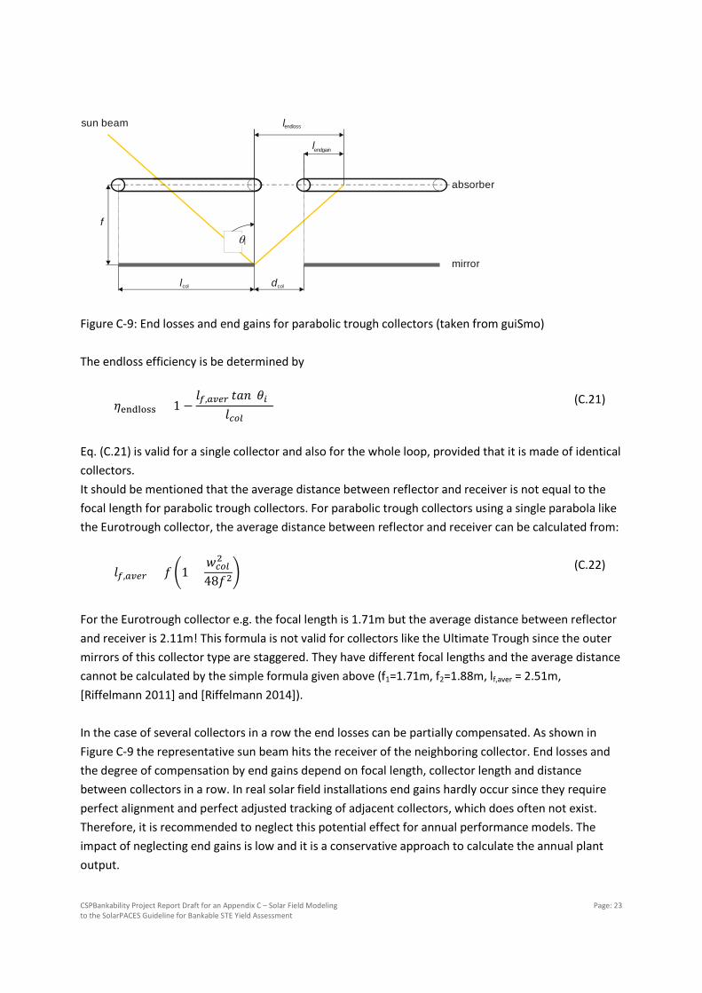
Figure C-9: End losses and end gains for parabolic trough collectors (taken from guiSmo) The endloss efficiency is be determined by 𝜂𝜂endloss = 1 −
𝑙𝑙𝑓𝑓,𝑡𝑡𝑎𝑎𝑠𝑠𝑡𝑡 𝑡𝑡𝑎𝑎𝑛𝑛(𝜃𝜃𝑎𝑎)𝑙𝑙𝑓𝑓𝑜𝑜𝑎𝑎
(C.21)
Eq. (C.21) is valid for a single collector and also for the whole loop, provided that it is made of identical collectors. It should be mentioned that the average distance between reflector and receiver is not equal to the focal length for parabolic trough collectors. For parabolic trough collectors using a single parabola like the Eurotrough collector, the average distance between reflector and receiver can be calculated from: 𝑙𝑙𝑓𝑓,𝑡𝑡𝑎𝑎𝑠𝑠𝑡𝑡 = 𝑓𝑓 �1 +
𝑤𝑤𝑓𝑓𝑜𝑜𝑎𝑎2
48𝑓𝑓2� (C.22)
For the Eurotrough collector e.g. the focal length is 1.71m but the average distance between reflector and receiver is 2.11m! This formula is not valid for collectors like the Ultimate Trough since the outer mirrors of this collector type are staggered. They have different focal lengths and the average distance cannot be calculated by the simple formula given above (f1=1.71m, f2=1.88m, lf,aver = 2.51m, [Riffelmann 2011] and [Riffelmann 2014]). In the case of several collectors in a row the end losses can be partially compensated. As shown in Figure C-9 the representative sun beam hits the receiver of the neighboring collector. End losses and the degree of compensation by end gains depend on focal length, collector length and distance between collectors in a row. In real solar field installations end gains hardly occur since they require perfect alignment and perfect adjusted tracking of adjacent collectors, which does often not exist. Therefore, it is recommended to neglect this potential effect for annual performance models. The impact of neglecting end gains is low and it is a conservative approach to calculate the annual plant output.
lcol dcol
lendgain
f
lendloss
mirror
sun beam
absorber
CSPBankability Project Report Draft for an Appendix C – Solar Field Modeling to the SolarPACES Guideline for Bankable STE Yield Assessment
Page: 24
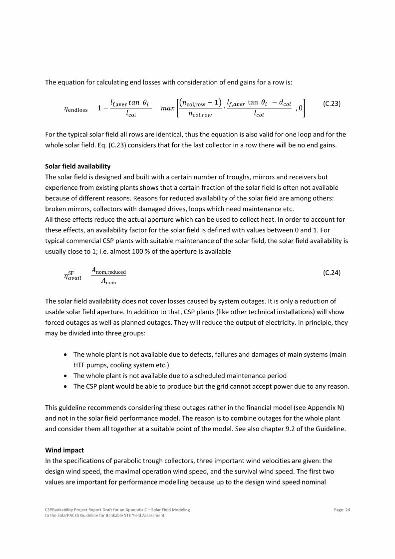
The equation for calculating end losses with consideration of end gains for a row is: 𝜂𝜂endloss = 1 −
𝑙𝑙f,aver 𝑡𝑡𝑎𝑎𝑛𝑛(𝜃𝜃𝑎𝑎)𝑙𝑙col
+ 𝑚𝑚𝑎𝑎𝑚𝑚 ��𝑛𝑛col,row − 1�
𝑛𝑛𝑓𝑓𝑜𝑜𝑎𝑎,𝑡𝑡𝑜𝑜𝑟𝑟∙𝑙𝑙𝑓𝑓,𝑡𝑡𝑎𝑎𝑠𝑠𝑡𝑡 tan(𝜃𝜃𝑎𝑎) − 𝑑𝑑𝑓𝑓𝑜𝑜𝑎𝑎
𝑙𝑙𝑓𝑓𝑜𝑜𝑎𝑎 , 0� (C.23)
For the typical solar field all rows are identical, thus the equation is also valid for one loop and for the whole solar field. Eq. (C.23) considers that for the last collector in a row there will be no end gains. Solar field availability The solar field is designed and built with a certain number of troughs, mirrors and receivers but experience from existing plants shows that a certain fraction of the solar field is often not available because of different reasons. Reasons for reduced availability of the solar field are among others: broken mirrors, collectors with damaged drives, loops which need maintenance etc. All these effects reduce the actual aperture which can be used to collect heat. In order to account for these effects, an availability factor for the solar field is defined with values between 0 and 1. For typical commercial CSP plants with suitable maintenance of the solar field, the solar field availability is usually close to 1; i.e. almost 100 % of the aperture is available 𝜂𝜂𝑡𝑡𝑎𝑎𝑡𝑡𝑎𝑎𝑎𝑎SF =
𝐴𝐴nom,reduced
𝐴𝐴nom (C.24)
The solar field availability does not cover losses caused by system outages. It is only a reduction of usable solar field aperture. In addition to that, CSP plants (like other technical installations) will show forced outages as well as planned outages. They will reduce the output of electricity. In principle, they may be divided into three groups:
• The whole plant is not available due to defects, failures and damages of main systems (main HTF pumps, cooling system etc.)
• The whole plant is not available due to a scheduled maintenance period • The CSP plant would be able to produce but the grid cannot accept power due to any reason.
This guideline recommends considering these outages rather in the financial model (see Appendix N) and not in the solar field performance model. The reason is to combine outages for the whole plant and consider them all together at a suitable point of the model. See also chapter 9.2 of the Guideline. Wind impact In the specifications of parabolic trough collectors, three important wind velocities are given: the design wind speed, the maximal operation wind speed, and the survival wind speed. The first two values are important for performance modelling because up to the design wind speed nominal

CSPBankability Project Report Draft for an Appendix C – Solar Field Modeling to the SolarPACES Guideline for Bankable STE Yield Assessment
Page: 25
efficiency should be reached. Above this design wind speed, presumably the efficiency of collectors will be reduced by induced oscillations and deformation of the reflecting surfaces, or tracking errors. Systematic research and models for this effect are hardly available today. Even if the wind impact on the optical performance is known for a single collector, it may change significantly in a large solar field with many other collectors, or when a wind breaker fence at the solar field boundaries is installed, etc. In order to consider this effect in annual performance models, more data from suppliers or independent laboratories must be available. On the other hand, each collector has a certain maximal operation wind velocity above which it must be turned into stow position in order to avoid damages. It is obvious that in these cases there will be no heat production and this effect should be considered in annual performance models. The survival wind speed has no impact on the performance but rather on the plant design. In order to estimate the impact of time periods with wind velocities between nominal and shut off wind speed, one example dataset has been analyzed in detail. Figure C-10 shows a plot of wind velocities over DNI for the 10 minutes TMY datasets for the PSA (Spain). From this plot, it is obvious that there is no correlation between wind speed and DNI. This conclusion is also valid for many other sites. On the other hand, summing up all DNI values for time periods with wind velocities above 7 m/s and below 14 m/s (that means between design wind speed and shut off wind speed) results in 308 kWh/m² which is about 14 % of the total DNI resource (2162 kWh/m²). This fraction shows that the wind impact on annual yield might actually be significant.
Figure C-10: Plot showing wind velocities over DNI for the TMY at PSA (Spain), 10 minutes mean values.
7
9
11
13
15
17
19
21
23
0 200 400 600 800 1000 1200
win
d sp
eed
in m
/s
DNI in W/m²
CSPBankability Project Report Draft for an Appendix C – Solar Field Modeling to the SolarPACES Guideline for Bankable STE Yield Assessment
Page: 26
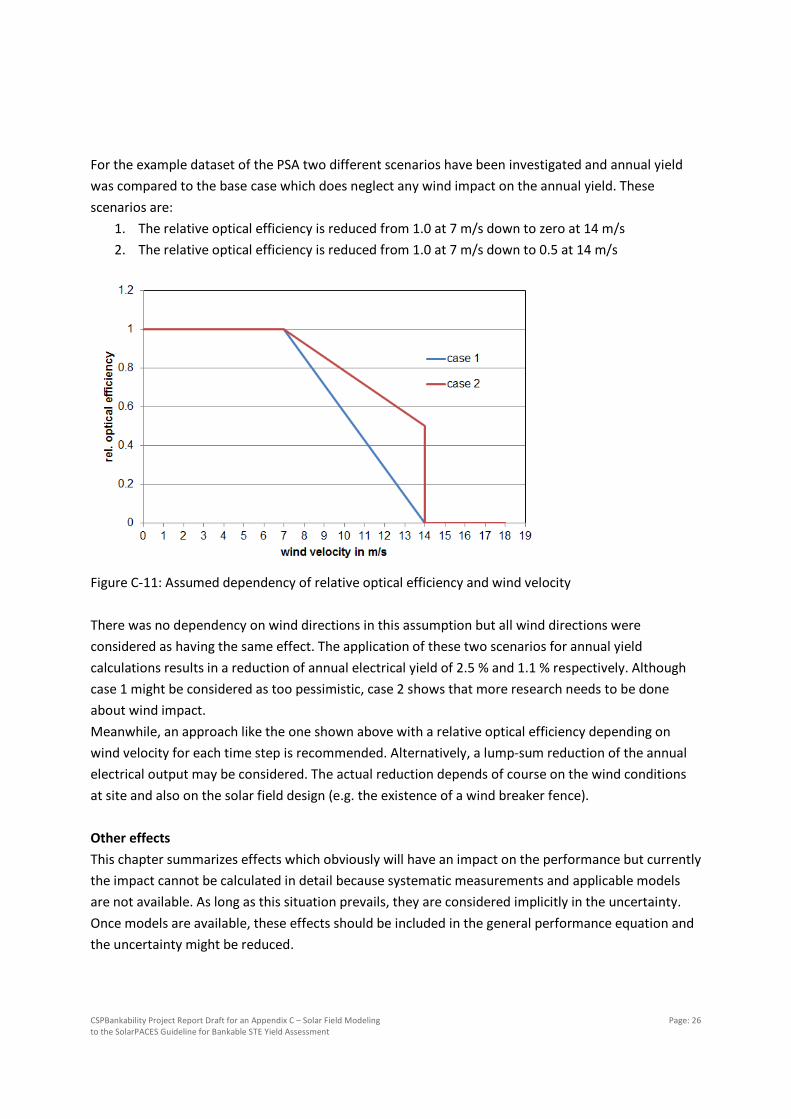
For the example dataset of the PSA two different scenarios have been investigated and annual yield was compared to the base case which does neglect any wind impact on the annual yield. These scenarios are:
1. The relative optical efficiency is reduced from 1.0 at 7 m/s down to zero at 14 m/s 2. The relative optical efficiency is reduced from 1.0 at 7 m/s down to 0.5 at 14 m/s
Figure C-11: Assumed dependency of relative optical efficiency and wind velocity There was no dependency on wind directions in this assumption but all wind directions were considered as having the same effect. The application of these two scenarios for annual yield calculations results in a reduction of annual electrical yield of 2.5 % and 1.1 % respectively. Although case 1 might be considered as too pessimistic, case 2 shows that more research needs to be done about wind impact. Meanwhile, an approach like the one shown above with a relative optical efficiency depending on wind velocity for each time step is recommended. Alternatively, a lump-sum reduction of the annual electrical output may be considered. The actual reduction depends of course on the wind conditions at site and also on the solar field design (e.g. the existence of a wind breaker fence). Other effects This chapter summarizes effects which obviously will have an impact on the performance but currently the impact cannot be calculated in detail because systematic measurements and applicable models are not available. As long as this situation prevails, they are considered implicitly in the uncertainty. Once models are available, these effects should be included in the general performance equation and the uncertainty might be reduced.

CSPBankability Project Report Draft for an Appendix C – Solar Field Modeling to the SolarPACES Guideline for Bankable STE Yield Assessment
Page: 27
Sun shape Direct normal irradiance today is measured by instruments with a certain acceptance angle which is about 10 times larger than the solar disk angle [Wilbert 2014]. Therefore, Gbn measurements contain a certain fraction of scattered radiation, which is called circumsolar radiation. This circumsolar radiation can only partially be used by concentrating collectors. Furthermore, it varies for different sites and is time dependent. The normalized radiance profile as function of the angular distance from the center of the sun is denoted as “sun shape” and [Wilbert 2014] has shown that the impact of the sun shape on annual yield of a trough plant might be an overestimation up to 0.5 to 1.1 % depending on the site. The lower value has been calculated for a Spanish site with lower circumsolar radiation and the upper value for Abu Dhabi with high circumsolar radiation. It should be mentioned that the reference was a disk sun shape with almost no circumsolar radiation. The annual yield calculations of [Wilbert 2014] are based on ray tracing simulations while the optical efficiency of parabolic trough collectors is typically determined under outdoor conditions. Thus, the measured optical efficiency of parabolic troughs already includes the sun shape effect at least for the conditions available during the measurement. This would reduce the overestimation mentioned above. Nevertheless, the sun shape during efficiency measurements for parabolic troughs is typically not reported in supplier’s datasheets and Wilbert’s results show that further investigation will be necessary; particularly for solar tower systems where the impact of sun shape is even higher. For some collectors, the optical efficiency is not measured but rather determined by ray tracing simulations. In this case, the annual performance simulation might even show an underestimation of up to 0.4 % when the actual sun shape at site has less circumsolar radiation than the sun shape used in the ray tracing model. Dew impact At many sites, the mirrors may be covered by dew in the morning which prevents reflection and thus heat production. Although this effect has been observed at several parabolic trough plants, there is currently no model available. Most of the existing meteorological stations at CSP sites do not monitor dew and it is not possible to calculate the occurrence simply from ambient temperature and humidity. Radiation between the mirror surface, sky and the environment is also important. Therefore, dew impact is currently neglected in annual performance models. Beside the “blindness” of mirrors, dew might have two more effects on solar fields: increased corrosion and increased adhesion of dust on the wet mirrors. Again models for these effects are currently not available. Snow impact Snow will not be an issue for many CSP sites but it may occur at some of them. Similar to dew, snow will also prevent reflection. The typical meteorological datasets do not mention snow, therefore it cannot be considered in the models. On the other hand it has been reported by plant operators, that snow provides a very effective cleaning of the mirrors.

CSPBankability Project Report Draft for an Appendix C – Solar Field Modeling to the SolarPACES Guideline for Bankable STE Yield Assessment
Page: 28
Table C-6 gives an overview about these effects which are currently not considered in the model as well as estimated about their impact on annual output. As long as no model details are available for them, the recommendation is to consider these effects in the uncertainty analysis (see chapter 9.3 of the Guideline). Table C-6: Effects not considered in the annual performance model Neglected effect Effective
direction Estimated impact on annual performance
Sun shape , +0.4….-1.1 % Dew impact 0….-0.5 % Snow impact 0….-0.5 %
C.2.1.3. Thermal losses
Thermal losses for a parabolic trough solar field can be divided into several individual effects and allocated to certain parts of the solar field. ��̇�𝑄loss = �̇�𝑄loss,rec + �̇�𝑄loss,pipe + �̇�𝑄loss,head + �̇�𝑄loss,equ (C.25)
With: �̇�𝑄loss,rec receiver heat losses in W �̇�𝑄loss,pipe heat losses of the loop piping in W �̇�𝑄loss,head header and runner heat losses in W �̇�𝑄loss,equ heat losses of other SF equipment (like tanks, vessels, etc.) in W Receiver thermal losses Parabolic trough collector fields are equipped with thousands of meters of receiver pipes to collect the concentrated irradiation and to enable heat transfer to the fluid as well as transportation of the fluid. These pipes experience thermal losses caused by the following three mechanisms: conduction, convection, and radiation. The receiver pipes are designed and manufactured in order to minimize thermal losses. They typically:
• have a selective coating to minimize radiative heat losses, • are equipped with a glass envelope enclosing the absorber pipe in vacuum to minimize
convective losses, • have small and insulated supports to minimize conductive losses.
Despite these measures the receiver heat losses are not negligible and induce a significant reduction of the net heat generation of parabolic trough solar fields. For state-of-the-art parabolic trough receivers, heat losses at nominal operating conditions are in the range of 10 % of the total heat absorbed.
CSPBankability Project Report Draft for an Appendix C – Solar Field Modeling to the SolarPACES Guideline for Bankable STE Yield Assessment
Page: 29
Unfortunately, standards about testing this kind of receivers and reporting test results are not available today. Therefore, several approaches exist in parallel and often they cannot be transformed easily into each other. Thermal receiver losses are often given as polynomial or lookup table and are provided by suppliers or published by laboratories. In the following chapter, several approaches are shown and discussed. Often, annual performance models must use what they get as input for receiver heat losses and the options for manipulation of the given equations are limited. The paragraphs show some pitfalls which must be obeyed when using or extending receiver heat loss equations from literature. [Dudley 1984] proposed a second order polynomial with an additional linear term containing Gbn in order to account for the fact that higher irradiance should have an impact on absorber surface temperatures. His model equations for specific receiver heat losses (in W/m of receiver length) are based on the bulk HTF temperature. �̇�𝑞loss,rec = 𝐼𝐼𝐴𝐴𝐼𝐼′ 𝐺𝐺bn𝑎𝑎0(𝜗𝜗𝐻𝐻𝐻𝐻𝐻𝐻 − 𝜗𝜗𝑡𝑡𝑎𝑎𝑎𝑎) + 𝑎𝑎1(𝜗𝜗𝐻𝐻𝐻𝐻𝐻𝐻 − 𝜗𝜗𝑡𝑡𝑎𝑎𝑎𝑎) + 𝑎𝑎2(𝜗𝜗𝐻𝐻𝐻𝐻𝐻𝐻 − 𝜗𝜗𝑡𝑡𝑎𝑎𝑎𝑎)2 (C.26) Most of the empirical heat loss equations cited in this chapter are written with temperatures in °C. In this handbook we recommend to use rather K but as long as temperature differences are used, both approaches are equivalent. [Burkholder 2009] cites the equation from [Price 2003] which is also used in the SAM empirical model. �̇�𝑞loss,rec = 𝑏𝑏0 + 𝑏𝑏1(𝜗𝜗𝐻𝐻𝐻𝐻𝐻𝐻 − 𝜗𝜗𝑡𝑡𝑎𝑎𝑎𝑎) + 𝑏𝑏2𝜗𝜗𝐻𝐻𝐻𝐻𝐻𝐻2 + 𝑏𝑏3𝜗𝜗𝐻𝐻𝐻𝐻𝐻𝐻3
+ 𝑏𝑏4𝐺𝐺bn𝐼𝐼𝐴𝐴𝐼𝐼 𝑐𝑐𝑐𝑐𝑐𝑐(𝜃𝜃𝑎𝑎)𝜗𝜗𝐻𝐻𝐻𝐻𝐻𝐻2 + �𝑣𝑣𝑟𝑟𝑎𝑎𝑡𝑡𝑠𝑠 �𝑏𝑏5 + 𝑏𝑏6(𝜗𝜗𝐻𝐻𝐻𝐻𝐻𝐻 − 𝜗𝜗𝑡𝑡𝑎𝑎𝑎𝑎)�
(C.27)
This equation considers the impact of HTF temperature (represented by b2 and b3), the impact of absorber temperature (b4), ambient temperature, and wind (represented by b1, b5 and b6). For evacuated receivers with intact glass covers, the impact of ambient conditions is small and the HTF temperature is the dominating parameter (Figure C-12 and Figure C-13). From Figure C-12 it is obvious that the function has a lower limit temperature below which the validity is questionable. The plotted curves show an intersection at about 150 °C which cannot be explained by physically means. [Burkholder 2009] calculated the coefficients of equation (C.27) using a model developed by [Forristall 2003] and fitting the parameters of this equation to heat loss measurements. The Forristall model needs additional input parameters like absorptance and emittance of the absorber and transmittance of the glass envelope. These values are not generally available, therefore a simpler approach must often be chosen.

CSPBankability Project Report Draft for an Appendix C – Solar Field Modeling to the SolarPACES Guideline for Bankable STE Yield Assessment
Page: 30
Figure C-12: Impact of wind velocity on receiver heat losses for a Schott PTR 70 receiver according to eq. (C.27) (Coefficients from [Burkholder 2009])
Figure C-13: Impact of beam irradiance on receiver heat losses for a Schott PTR 70 receiver according to eq. (C.27) (Coefficients from [Burkholder 2009]) Currently, thermal receiver tests are typically performed in laboratories by heating a single receiver electrically from inside to a certain temperature and measure the heat losses for this stagnant temperature. The test results are reported typically as an approximating equation for the measured specific heat losses per meter of receiver tube with the receiver temperature as independent
0
50
100
150
200
250
300
350
400
0 100 200 300 400 500
heat
loss
in W
/m
ϑHTF in °C
v_w = 0 m/s
v_w = 12 m/s
0
50
100
150
200
250
300
350
400
0 100 200 300 400 500
heat
loss
in W
/m
ϑHTF in °C
G_bn = 200 W/m²
G_bn = 1000 W/m²

CSPBankability Project Report Draft for an Appendix C – Solar Field Modeling to the SolarPACES Guideline for Bankable STE Yield Assessment
Page: 31
parameter. This function is often a polynomial up to fourth order since radiation is the dominating heat loss effect and a fourth order equation provides often good approximation for the measurements. �̇�𝑞loss,rec = 𝑎𝑎0 + 𝑎𝑎1(𝜗𝜗𝑡𝑡𝑎𝑎𝑡𝑡 − 𝜗𝜗𝑡𝑡𝑎𝑎𝑎𝑎) + 𝑎𝑎2(𝜗𝜗𝑡𝑡𝑎𝑎𝑡𝑡 − 𝜗𝜗𝑡𝑡𝑎𝑎𝑎𝑎)2 + 𝑎𝑎3(𝜗𝜗𝑡𝑡𝑎𝑎𝑡𝑡 − 𝜗𝜗𝑡𝑡𝑎𝑎𝑎𝑎)3
+ 𝑎𝑎4(𝜗𝜗𝑡𝑡𝑎𝑎𝑡𝑡 − 𝜗𝜗𝑡𝑡𝑎𝑎𝑎𝑎)4 (C.28)
Today, laboratory tests are often just using the following equation for specific heat losses [Burkholder 2009], [Pernpeintner 2012]: �̇�𝑞loss,rec = 𝑎𝑎1𝜗𝜗abs + 𝑎𝑎2𝜗𝜗𝑡𝑡𝑎𝑎𝑡𝑡4 (C.29) This equation has two problems considering the direct utilization in annual performance models: the utilization of the absorber temperature rather than the bulk fluid temperature and the missing dependency on ambient temperature. One argument for the latter simplification is that all measurements are done at the same ambient temperature and that this ambient temperature is quite low compared to the absorber temperature (at nominal conditions). Laboratory measurements of receiver heat losses like those reported in [Burkholder 2009] are made with an electrical heating element inside the absorber tubes. The absorber temperature at the inner side is measured together with the electrical power needed to keep the whole tube at this temperature at steady state conditions. In an operating parabolic trough plant the absorber surface temperature will not be the same as the bulk HTF temperature. A certain part of the absorber circumference will be hit by concentrated sunlight and may have a higher temperature than the bulk HTF. The remaining part of the absorber circumference might show lower temperatures. Annual performance models will rather use the bulk HTF temperature of the fluid instead of the absorber surface temperature in order to simplify the calculation. [Burkholder 2009] has calculated a temperature difference of 1 to 4 K between the inner side of the absorber tube and the bulk fluid temperature dependent on the beam irradiance. The higher value of 4 K has been calculated for Gbn=800 W/m² and using the laboratory heat loss curve assuming that bulk fluid temperature and inner absorber temperature are identical would result in an underestimation of heat losses of 3.4 % at 350 °C mean fluid temperature for the DPO/BP system. [Duffie 1991] and [Lüpfert 2004] propose to use a heat loss efficiency factor F’ to account for the temperature difference between bulk HTF and wall temperature and write the heat loss equation with the temperature difference between bulk fluid and ambient. The physical interpretation of this efficiency factor is the ratio of the total heat transfer coefficient from fluid to ambient to the heat transfer coefficient from absorber tube to ambient. With this factor equation (C.28) becomes: �̇�𝑞loss,rec = 𝐹𝐹′ ∙ [𝑎𝑎0 + 𝑎𝑎1(𝜗𝜗𝐻𝐻𝐻𝐻𝐻𝐻 − 𝜗𝜗𝑡𝑡𝑎𝑎𝑎𝑎) + 𝑎𝑎2(𝜗𝜗𝐻𝐻𝐻𝐻𝐻𝐻 − 𝜗𝜗𝑡𝑡𝑎𝑎𝑎𝑎)2 + 𝑎𝑎3(𝜗𝜗𝐻𝐻𝐻𝐻𝐻𝐻 − 𝜗𝜗𝑡𝑡𝑎𝑎𝑎𝑎)3
+ 𝑎𝑎4(𝜗𝜗𝐻𝐻𝐻𝐻𝐻𝐻 − 𝜗𝜗𝑡𝑡𝑎𝑎𝑎𝑎)4] (C.30)
CSPBankability Project Report Draft for an Appendix C – Solar Field Modeling to the SolarPACES Guideline for Bankable STE Yield Assessment
Page: 32
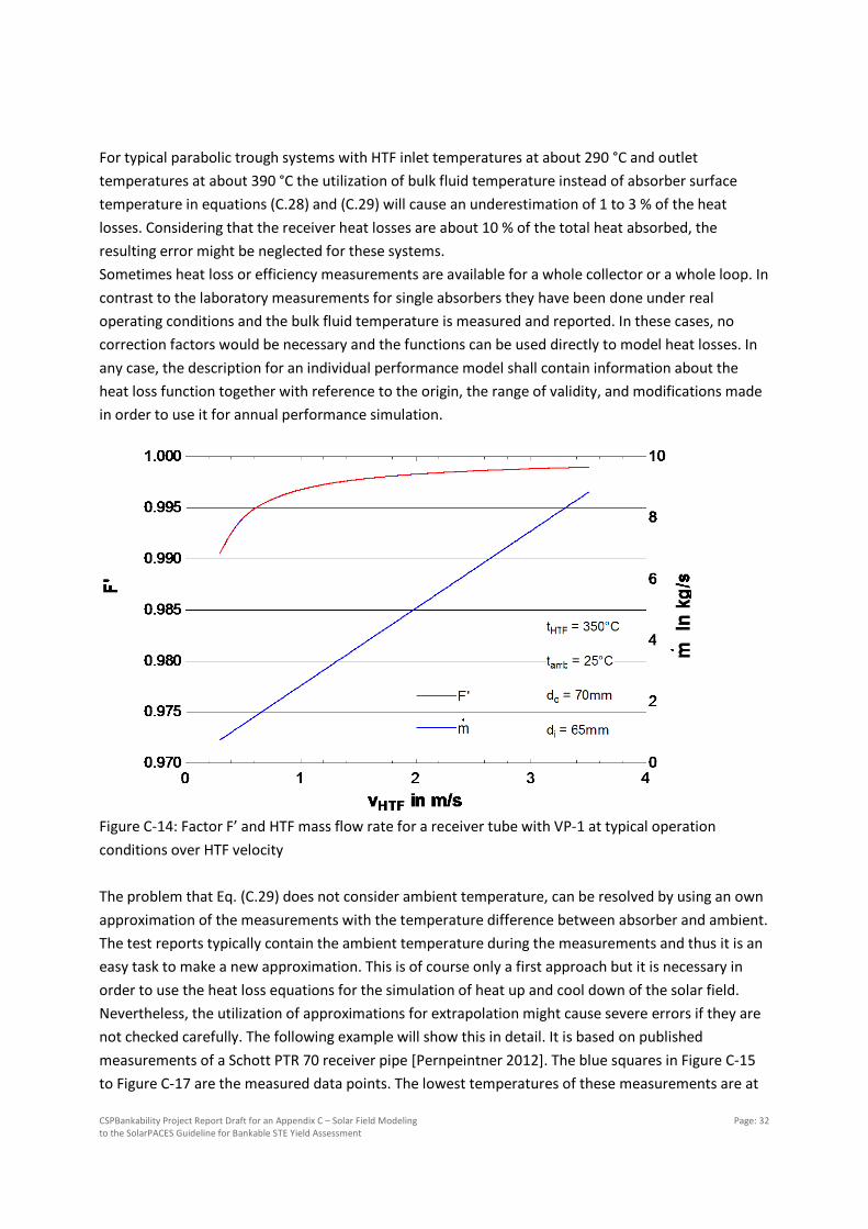
For typical parabolic trough systems with HTF inlet temperatures at about 290 °C and outlet temperatures at about 390 °C the utilization of bulk fluid temperature instead of absorber surface temperature in equations (C.28) and (C.29) will cause an underestimation of 1 to 3 % of the heat losses. Considering that the receiver heat losses are about 10 % of the total heat absorbed, the resulting error might be neglected for these systems. Sometimes heat loss or efficiency measurements are available for a whole collector or a whole loop. In contrast to the laboratory measurements for single absorbers they have been done under real operating conditions and the bulk fluid temperature is measured and reported. In these cases, no correction factors would be necessary and the functions can be used directly to model heat losses. In any case, the description for an individual performance model shall contain information about the heat loss function together with reference to the origin, the range of validity, and modifications made in order to use it for annual performance simulation.
Figure C-14: Factor F’ and HTF mass flow rate for a receiver tube with VP-1 at typical operation conditions over HTF velocity The problem that Eq. (C.29) does not consider ambient temperature, can be resolved by using an own approximation of the measurements with the temperature difference between absorber and ambient. The test reports typically contain the ambient temperature during the measurements and thus it is an easy task to make a new approximation. This is of course only a first approach but it is necessary in order to use the heat loss equations for the simulation of heat up and cool down of the solar field. Nevertheless, the utilization of approximations for extrapolation might cause severe errors if they are not checked carefully. The following example will show this in detail. It is based on published measurements of a Schott PTR 70 receiver pipe [Pernpeintner 2012]. The blue squares in Figure C-15 to Figure C-17 are the measured data points. The lowest temperatures of these measurements are at

CSPBankability Project Report Draft for an Appendix C – Solar Field Modeling to the SolarPACES Guideline for Bankable STE Yield Assessment
Page: 33
227 °C above ambient. The annual performance model will need to calculate heat losses at significant lower temperature differences for night time cooling down simulation. Thus approximations were made in order to get an equation which might be used for the whole temperature range from ambient temperature up to maximum absorber temperature. From Figure C-15 it is obvious that a second order polynomial is not suitable whereas Figure C-16 shows that the 4th order polynomial, which goes through the origin, might be a reasonable approximation in this case. Further constraints might be used to get a physically meaningful approximation: first and second derivatives should be always larger than zero in the relevant temperature range.
Figure C-15: Approximation of receiver heat losses by 2nd order polynomials
Figure C-16: Approximation of receiver heat losses by 4th order polynomials
-50
0
50
100
150
200
250
300
0 100 200 300 400 500
spec
ific
heat
loss
in W
/m
absorber temperature above ambient in °C
Measurement
2nd order through origin
2nd order not through origin
-50
0
50
100
150
200
250
300
0 100 200 300 400 500
spec
ific
heat
loss
in W
/m
absorber temperature above ambient in °C
Measurement
4th order through origin
4th order not through origin

CSPBankability Project Report Draft for an Appendix C – Solar Field Modeling to the SolarPACES Guideline for Bankable STE Yield Assessment
Page: 34
Figure C-17 shows that a spline approximation will be even better in the sense that it will meet the measurements. This example shows that the user must be very cautious when using approximations for extrapolation and check that the approximation will give physically reasonable results for the whole temperature range. In general, it would be desirable to get more measurements also for low absorber temperatures from the modeler’s point of view.
Figure C-17: Approximation of receiver heat losses by splines Another important question is whether one single mean temperature between solar field inlet and outlet would be sufficient to model the heat losses or whether more nodes are necessary. [Wittmann 2012] published a paper on this topic, concluding that the underestimation of heat losses for typical parabolic trough systems with thermal oil and 290 °C/390 °C temperatures is in the range of 3-5 % when using just one single mean temperature. Again, this might be negligible for annual performance simulations since the impact on annual thermal output will be an over estimation in the range of 0.5 %. For parabolic trough systems with considerable higher outlet temperature and temperature rise, [Wittmann 2012] proposes the utilization of a correction factor when using a single temperature node over the whole loop for heat loss calculation. �̇�𝑞loss,corr = 𝑓𝑓corr ∙ �̇�𝑞loss,rec (C.31) The correction factor 𝑓𝑓corr may be calculated for the specific system in a separate model with high spatial resolution for the whole loop. Main parameters for the correction factor are beam irradiance and inlet and outlet temperature of the loop, thus the correction factor will depend on solar field load.
-50
0
50
100
150
200
250
300
0 100 200 300 400 500
spec
ific
heat
loss
in W
/m
absorber temperature above ambient in °C
Measurement
Spline approximation
4th order through origin

CSPBankability Project Report Draft for an Appendix C – Solar Field Modeling to the SolarPACES Guideline for Bankable STE Yield Assessment
Page: 35
Thermal losses of field piping and header system In parabolic trough solar fields, the individual troughs must be connected to each other by pipes and flexible connectors. These connectors may be flexible hoses or so called ball joints and they allow for individual tracking of each single collector as well as for longitudinal expansion of the receiver pipes. Crossover pipes connect two collector rows to form a U-type loop and loops are connected by interconnecting pipes to the headers, which in turn are connected with runners. Furthermore, each loop has a number of valves for isolation, draining or venting as well as flow distribution. “Runner” pipes connect the headers with heat exchangers, which are located near the turbine. All this equipment is called "field piping" and although they are well insulated, heat losses cannot be avoided. Thermal losses for field piping and headers can be calculated by detailed models from pipe diameters, HTF masses and temperatures, type and thickness of heat insulation, etc. but often it is sufficient to consider overall heat losses in terms of watt per square meter of aperture and mean temperature difference between solar field and ambient. Another option is to define specific piping losses per length unit as for the receiver heat losses. This approach is shown in (C.32) which gives an expression for the heat losses of a single loop. �̇�𝑄𝑎𝑎𝑜𝑜𝑡𝑡𝑡𝑡,𝑎𝑎𝑜𝑜𝑜𝑜𝑜𝑜 = 𝑛𝑛𝑓𝑓𝑜𝑜𝑎𝑎𝑎𝑎,𝑎𝑎𝑜𝑜𝑜𝑜𝑜𝑜 𝑛𝑛𝑡𝑡𝑠𝑠𝑓𝑓,𝑓𝑓𝑜𝑜𝑎𝑎𝑎𝑎 𝑙𝑙rec �̇�𝑞loss,rec + 𝑙𝑙𝑜𝑜𝑎𝑎𝑜𝑜𝑠𝑠,𝑎𝑎𝑜𝑜𝑜𝑜𝑜𝑜 �̇�𝑞loss,pipe (C.32) The typical piping length for one loop made of four Eurotrough 150 collectors is about 60-70m (including swivel joints, cross over pipe, connecting pipes to headers and valves but excluding the receivers). Piping heat losses depend of course on insulation material and thickness but a first approximation for these loop piping heat losses gives 150 to 200 W/m specific heat loss, assuming an insulation layer of 40 mm thickness for a 73 mm OD (2½’’) tube and heat conductivity of 0.07 W/(m K). These values are valid for ideal conditions of insulated pipes. The steady state net thermal power of one loop may be calculated from: �̇�𝑄loop,steady = 𝑐𝑐𝑐𝑐𝑐𝑐(𝜃𝜃𝑎𝑎) 𝐼𝐼𝐴𝐴𝐼𝐼 𝜂𝜂opt,0 𝜂𝜂shad 𝜂𝜂clean 𝑓𝑓focA 𝐴𝐴nom,loop 𝐺𝐺bn
− 𝑛𝑛coll, loop 𝑛𝑛rec, Coll 𝑙𝑙rec �̇�𝑞loss,rec − 𝑙𝑙pipe,loop �̇�𝑞loss,pipe (C.33)
Headers and runners might be considered in one single expression; therefore the header losses shall comprise both heat losses in headers as well as in runners. Header losses can be defined as specific heat losses per meter of header length and in this case they are in the same range as the piping losses given above, thus 150 to 200 W/m. Again these values are valid for ideal conditions of insulated pipes. The larger diameters of these header pipes require thicker insulation layers which results in similar specific heat losses than for the loop piping. Similarly higher fluid temperatures inside hot headers compared to cold headers may be compensated by thicker or better insulation layers. These values for piping and header heat losses are only given for information. During the detailed engineering phase a techno economic optimization will be done in order to determine the insulation thickness. For some CSP projects, maximum acceptable piping heat losses are defined in the technical specifications of
CSPBankability Project Report Draft for an Appendix C – Solar Field Modeling to the SolarPACES Guideline for Bankable STE Yield Assessment
Page: 36
tender documents. In this case, the value may be used as model input and the EPC contractor has to design the insulation in a manner that they are not exceeded. Another option is to define piping and header losses based on the aperture area. In this case, corresponding specific values are 3 to 4 W/m² for loop piping losses and additional 2 to 4 W/m² for header losses (provided that collector technology and solar field layout are similar to the parabolic trough with thermal oil reference plant). These values are valid for ideal conditions of insulated pipes. In a real plant the heat losses are higher because of the need for pipe support structures were additional heat losses caused by thermal conduction occur. Furthermore, the insulation might have defects or gaps, etc. Due to these non-ideal conditions the theoretical heat losses given above shall be multiplied by a factor of 1.5 to 2 in order to adapt them to real conditions according to a typical engineering guess. Thus we have 6 to 8 W/m² for loop piping losses and another 4 to 8 W/m² for header losses for nominal conditions. �̇�𝑄loss,head = 𝐴𝐴SF �̇�𝑞loss,head,A = 𝑙𝑙head �̇�𝑞loss,head (C.34) In principle, it must be mentioned which aperture definition is used for the calculation of these specific heat losses: net aperture, nominal aperture or gross aperture. Actually the values of these 3 aperture definitions will not be too different from each other but will rather be within a range of about 5 %. Since the utilization of aperture specific heat losses is an approximation and a simplification, the impact of aperture definition might be neglected and the values mentioned above may be used for each of the aperture definitions. The safety margin used above for aperture specific header and piping losses will cover these small differences in aperture area definitions. The idea behind the utilization of aperture specific heat losses (based on solar field aperture area) is that they allow for easy variation of the solar field size and scaling header and runner heat losses just by multiplying the specific heat losses and the actual solar field aperture instead of calculating the actual header length for each configuration. Such specific header losses based on aperture area are only valid within a certain range of aperture areas and it is not correct to use the same values for very small and very large solar fields. In these extreme cases the dependency of header length and diameter on solar field size and shape must be considered when using aperture specific heat losses. These values given above for specific piping and header losses are valid for nominal conditions. In order to use them also for heating up and cooling down during time periods without irradiance, they can be scaled linearly with the temperature difference between mean nominal solar field temperature and ambient temperature. �̇�𝑄𝑎𝑎𝑜𝑜𝑡𝑡𝑡𝑡,𝑜𝑜𝑎𝑎𝑜𝑜𝑠𝑠 = 𝑙𝑙pipe �̇�𝑞loss,pipe = 𝑙𝑙pipe �̇�𝑞loss,pipe,nom
(𝑇𝑇𝐻𝐻𝐻𝐻𝐻𝐻 − 𝑇𝑇𝑡𝑡𝑎𝑎𝑎𝑎)�𝑇𝑇𝐻𝐻𝐻𝐻𝐻𝐻,𝑡𝑡𝑜𝑜𝑎𝑎 − 𝑇𝑇𝑡𝑡𝑎𝑎𝑎𝑎,𝑡𝑡𝑜𝑜𝑎𝑎�
(C.35)
It is obvious that header losses will cause a certain temperature decrease. The highest HTF temperature occurs at the loop outlet and due to the header losses the inlet temperature to the HTF-

CSPBankability Project Report Draft for an Appendix C – Solar Field Modeling to the SolarPACES Guideline for Bankable STE Yield Assessment
Page: 37
steam heat exchangers is a few Kelvin lower than the average loop outlet temperature. The HTF temperature at the heat exchangers may be calculated with the specific heat capacity c of the fluid from �̇�𝑄loss,hot head = �̇�𝑚HTF 𝑐𝑐HTF�𝑇𝑇loop,out − 𝑇𝑇out
SF � (C.36) This equation shows that the temperature difference depends on the HTF mass flow rate and thus on the solar field load. Assuming a constant header heat loss, the temperature at the solar field outlet (which is identical to the temperature at heat exchanger inlet) decreases with decreasing mass flow. Similarly, the loop inlet temperature is typically lower than the HTF temperature at the solar field inlet (heat exchanger outlet). �̇�𝑄loss,cold head = �̇�𝑚HTF 𝑐𝑐HTF�𝑇𝑇in
SF − 𝑇𝑇loop,in� (C.37) Having the temperature drop in the cold and hot header in mind, the question arises, if the mean temperature calculated from solar field inlet and outlet temperature is representative for the receiver heat losses. Despite this temperature decrease, heat losses of the representative loop of the solar field (with single phase HTF and temperatures of about 290/390 °C) can be calculated with the mean solar field temperature which was calculated using the temperatures at the interface between solar field and heat exchangers. The justification for this approach is that the temperature decrease in both headers is almost the same and thus the arithmetic mean temperature between inlet and outlet is also the same, either using the temperatures at loop inlet or at the heat exchangers (Figure C-18). The impact of this simplification on the mean solar field temperature is only in the range of 0.5 to 1 K. The higher temperature difference between hot header and ambient is typically compensated by better or thicker insulation of this header compared to the cold header.

CSPBankability Project Report Draft for an Appendix C – Solar Field Modeling to the SolarPACES Guideline for Bankable STE Yield Assessment
Page: 38
Figure C-18: Temperature profile from pump inlet to solar field outlet in a large parabolic trough plant for 2 load cases. Heat gains Heat gains for parabolic trough solar fields are mainly caused by the pressure loss and by trace heating elements if such elements exist in the plant considered. ��̇�𝑄gain = �̇�𝑄Δ𝑜𝑜 + �̇�𝑄TH (C.38)
Thermal gain from pumps Main solar field pumps are large electricity consumers and as other technical equipment they are not perfect. Only a certain fraction of the electricity used by them is actually transferred into pressure increase. About 20 % (the actual value depends on the pump efficiency) of the electric consumption is dissipated at the pump and mainly increases the HTF temperature between pump inlet and outlet. �̇�𝑄pump = (1 − 𝜂𝜂𝑃𝑃) 𝑃𝑃el,P = �̇�𝑚HTF 𝑐𝑐HTF �𝑇𝑇𝑜𝑜𝑝𝑝𝑎𝑎𝑜𝑜,𝑜𝑜𝑝𝑝𝑡𝑡 − 𝑇𝑇𝑜𝑜𝑝𝑝𝑎𝑎𝑜𝑜,𝑎𝑎𝑡𝑡� (C.39) This is the thermal power which is directly supplied to the HTF at the pumps and this will lead to a slightly increased inlet temperature. The pressure loss of the solar field means that this energy is dissipated into heat too and must be considered in the energy balance since the electric power needed might be in the range of 2 % of the plants gross electrical annual output. �̇�𝑄∆p = ∆𝑝𝑝 105
Pabar
�̇�𝑚HTF
𝜌𝜌𝐻𝐻𝐻𝐻𝐻𝐻 (C.40)
200
220
240
260
280
300
320
340
360
380
400
0 500 1000 1500 2000 2500 3000 3500 4000 4500
tem
pera
ture
in �
C
distance from pump inlet in m
design load
20% load
cold header hot header
loop

CSPBankability Project Report Draft for an Appendix C – Solar Field Modeling to the SolarPACES Guideline for Bankable STE Yield Assessment
Page: 39
This is an additional heat input for the solar field (see Eq. (C.41)). Balance equation for the whole solar field With all the effects explained in the section above Eq. (C.4) becomes: �̇�𝑄steady
SF = �𝑛𝑛loops�𝐼𝐼𝐴𝐴𝐼𝐼 𝜂𝜂opt,0 𝜂𝜂shad 𝜂𝜂clean 𝑓𝑓focA 𝐴𝐴nom,loop 𝐺𝐺pr
− 𝑛𝑛Coll, loop 𝑛𝑛Abs, Coll 𝑙𝑙Abs �̇�𝑞loss,rec − 𝑙𝑙pipe,loop �̇�𝑞loss,pipe� − 𝑙𝑙header �̇�𝑞loss,head + �̇�𝑄∆𝑜𝑜�
(C.41)
C.2.1.4. Pressure loss
The flow of HTF through receivers, headers, heat exchangers, pipe fittings and valves etc. leads to losses of flow energy due to irreversible processes which can be denoted as pressure losses. These losses may occur by friction, vortex shedding and secondary flow, whereas flow energy is always converted into heat. The solar field model must be capable to calculate these losses since main HTF pumps have to provide this pressure difference (plus the pressure difference caused by the solar steam generators and the storage heat exchangers). During detailed engineering of a CSP plant, dimensioning of piping and headers follows a techno-economic optimization since there is always a trade-off between minimal pressure loss and minimal HTF and steel masses. There are two different modeling approaches:
1. Calculation or estimation of pressure losses for design conditions and scaling with solar field thermal load.
2. Individual pressure loss calculation for every time instance. The first approach is often used in annual performance models. Pressure drop calculation for pipes, fittings, valves, etc. can be found in textbooks. For the reference systems the nominal pressure drop is given in Appendix B. Pressure loss of single phase fluid systems is proportional to the square of fluid velocity. ∆p~𝑣𝑣𝐻𝐻𝐻𝐻𝐻𝐻2 (C.42) Therefore, a quadratic scaling law for pressure drop may be applied in part load conditions.
∆p = ∆𝑝𝑝nom ��̇�𝑉HTF
�̇�𝑉HTF,nom�2
= ∆𝑝𝑝nom � �̇�𝑚HTF ∙ 𝜌𝜌HTF,nom
𝜌𝜌HTF ∙ �̇�𝑚HTF,nom �2
(C.43)

CSPBankability Project Report Draft for an Appendix C – Solar Field Modeling to the SolarPACES Guideline for Bankable STE Yield Assessment
Page: 40
C.2.1.5. Auxiliary electrical consumption
The solar field needs electrical power for pumping, control, etc. which may be divided into two fractions: One fraction depends on load and/or solar field state and ambient conditions and the second one is constant. The auxiliary demand of the solar field will be different for periods with and without irradiance but in general, even during times without usable irradiance, there will be a certain electricity demand. 𝑃𝑃auxSF = 𝑃𝑃aux,var
SF + 𝑃𝑃aux,fixSF (C.44)
In addition to the pumping power to overcome the pressure losses, the solar field has typically further electrical consumers:
• drives used to turn the parabolic troughs and for tracking the sun • instrumentation and control devices • trace heating of pipes and vessels which need freeze protection
The bullet points above show that the electrical consumers of a solar field may be divided into several groups:
• Equipment with load dependent consumption (e.g. main HTF pumps) • Equipment with almost constant consumption when the solar field is in operation (e.g.
tracking drives, auxiliary consumers of the HTF system) • Equipment with almost constant consumption when the solar field is out of operation (e.g.
those parts of I&C which are used for continuous monitoring) • Equipment which is only used under special conditions (e.g. trace heating, freeze protection
pumps or solar field recirculation pumps) Therefore, the electric power consumption of the solar field depends on the status of the solar field itself2:
𝑃𝑃el,onSF = 𝑃𝑃pump,nom � �̇�𝑚HTF ∙ 𝜌𝜌HTF,nom
𝜌𝜌HTF ∙ �̇�𝑚HTF,nom �2
+ 𝑃𝑃fix,onSF
(C.45)
With the base load auxiliary consumption of the solar field when the solar is in operation: 𝑃𝑃BL,on
SF . The nominal power of the main HTF pumps can be calculated from the nominal pressure loss. 𝑃𝑃pump,nom =
Δ𝑝𝑝𝑡𝑡𝑜𝑜𝑎𝑎 �̇�𝑉𝐻𝐻𝐻𝐻𝐻𝐻,𝑡𝑡𝑜𝑜𝑎𝑎
𝜂𝜂𝑃𝑃= Δ𝑝𝑝𝑡𝑡𝑜𝑜𝑎𝑎 �̇�𝑚𝐻𝐻𝐻𝐻𝐻𝐻,𝑡𝑡𝑜𝑜𝑎𝑎
𝜂𝜂𝑃𝑃 𝜌𝜌𝐻𝐻𝐻𝐻𝐻𝐻,𝑡𝑡𝑜𝑜𝑎𝑎 (C.46)
2 Update is in preparation taking into account the specific part-load behavior of the pumps

CSPBankability Project Report Draft for an Appendix C – Solar Field Modeling to the SolarPACES Guideline for Bankable STE Yield Assessment
Page: 41
If the solar field is not in operation the power is reduced to the constant offline auxiliary consumption and eventually the power consumption of recirculation pumps: 𝑃𝑃el,off
SF = 𝑃𝑃fix,offSF + 𝑃𝑃reci (C.47)
The mean electrical own consumption of one collector drive for a parabolic trough collector of about 150 m length and 5.77 m aperture width is in the range of 23 W when the collector is tracking and in the range of 3 W in stow position. These values are valid for collector equipped with hydraulic drives with individual drives for each collector. The actual instantaneous electrical power of these hydraulic pumps is higher but they are only operated temporarily.
C.2.1.6. Losses caused by operational limits
In a real CSP plant most of the installed technical equipment has well defined limits for operation and sometimes the limit of one single part restricts the output of the whole plant. These limits are mainly:
• Minimum operation limit: Many parts of the solar field (receivers, pumps, heat exchangers, etc.) have a minimum fluid flow in order to maintain stable working conditions, thus not every sun beam can be used for plant operation.
• Maximum operation limit: The same is valid for maximum flows, temperature limits etc. • The thermal storage has a limited capacity and during sunny summer days it might be totally
charged prior to sunset. • Maximum wind velocity (or rather gusts): Collectors and heliostats sustain a certain upper
wind speed for operation (provided by suppliers). Above that wind speed they must be turned into stow position in order to avoid damages. Time periods with high irradiation and high wind velocity can thus not be accounted for production.
• Some parts of the plant (particularly heat exchangers and steam turbine) have restrictions for heating-up or cooling down.
Above mentioned limits may reduce the actual output of the solar field and a fraction of the available solar energy cannot be utilized. In annual performance models it is important to define and report these limits in order to obtain comparable results. The solar field model must provide interface variables as output specifying the minimum and maximum HTF mass flow rate. These values might be constant or variable from time step to step, depending on the actual plant design. The fraction of the theoretical solar field heat output which could be produced but actually cannot be used due to operational limits is called defocussed energy. The annual sum of defocussed energy should be reported since it can be used to evaluate the design of a CSP plant.

CSPBankability Project Report Draft for an Appendix C – Solar Field Modeling to the SolarPACES Guideline for Bankable STE Yield Assessment
Page: 42
C.2.1.7. Transient effects
All models in chapter C.2 are valid for steady state operation and the overall modeling approach is also a steady state model with constant input and output for individual time steps. Nevertheless the goal is to predict the annual output of power plants with large fluctuations of the main input parameter DNI, which may be considered as the driving “fuel”. The steady state model does not consider that startup and load variation is not instantaneous but requires certain time. Equation (C.1) contains an additional part to consider transient effects �̇�𝑄trans. The major and dominating transient effect of the solar field is its thermal inertia. The yield calculation is influenced by thermal effects which are initiated during plant start-up and shut down and during cloud effects by which the solar energy input changes rapidly. The change of energy input during a clear sky day due to the normal increase and decrease of the DNI levels and due to the changing incidence angle can be seen as subordinated to the aforementioned causes. Changes of operating states are slow; the operating states can be considered as a sequence of stationary conditions. Parabolic trough solar fields contain large amounts of HTF (typically more than 3000 tons for a 100 MWe plant with storage) and steel pipes with direct contact to HTF (this steel mass is in the same order of magnitude as for HTF mass). During the night and hours without DNI, this solar field inventory cools down and must be heated up again to nominal operating conditions before the next operation phase can begin. During this period the solar field does not deliver any “useful” heat which could be used to charge the storage or to operate the power block. Instead the collected heat is mainly utilized to increase the temperature of the solar field itself. On the other hand thermal inertia of the solar field may be used to operate the power block for a certain time period even after the irradiation disappears. Typically the heat which has to be put into the system during startup is higher than the heat which can be recovered after sunset since the solar field will cool down during the whole night and the heat stored in HTF and piping can only be utilized down to a certain temperature. Sometimes it is even not desired to utilize this heat but rather use it to keep the temperature in the system at a higher level in order to reduce startup time in the next morning. The actual practice depends on the design of the plant and the operating concept. Clouds may shade parts of the solar field or even the whole solar field for a short time period, causing fluctuations in heat output, either temperature or mass flow fluctuations or both. In extreme situations this might be so pronounced that the power block cannot be operated though the mean DNI over a time period of one hour would be sufficient. The steady state thermal output of the solar field may be reduced by transient effects, thus the solar field net thermal energy which can be delivered to power block and/or thermal storage in a time step is: 𝑄𝑄𝑆𝑆𝐻𝐻 = ��̇�𝑄𝑡𝑡𝑡𝑡𝑠𝑠𝑡𝑡𝑠𝑠𝑠𝑠𝑆𝑆𝐻𝐻 ∙ Δ𝑡𝑡 − 𝑄𝑄heatup� ∙ 𝜉𝜉cloud (C.48) Equation (C.48) is written in terms of thermal energy rather than thermal power since heating up and net heat production may occur in the same time step but not simultaneously. The factor 𝜉𝜉cloud is

CSPBankability Project Report Draft for an Appendix C – Solar Field Modeling to the SolarPACES Guideline for Bankable STE Yield Assessment
Page: 43
introduced to account for losses caused by clouds. Its value is between 0 and 1.0 and may vary from time step to time step. Currently it should be set to 1.0, neglecting losses caused by transients due to clouds because there is no validated model available. Once appropriate models are available the factor may be calculated and used to correct the solar field output. The heat required for startup or provided by the HTF and steel mass during cool down may be calculated from: 𝑄𝑄inertia,ideal
SF = �𝑚𝑚𝐻𝐻𝐻𝐻𝐻𝐻 ∙ 𝑐𝑐𝐻𝐻𝐻𝐻𝐻𝐻 +𝑚𝑚𝑜𝑜𝑎𝑎𝑜𝑜𝑠𝑠 ∙ 𝑐𝑐pipe��𝑇𝑇�𝐻𝐻𝐻𝐻𝐻𝐻 − 𝑇𝑇�𝐻𝐻𝐻𝐻𝐻𝐻,𝑡𝑡−Δt� (C.49) This equation accounts for the heat capacity of HTF inventory and the heat capacity of the piping in contact with the fluid. The latter value can be found by calculating the steel mass present in the solar field and might therefore be difficult to determine; thus another option would be to use solely the HTF heat capacity and multiply it by a factor bh> 1. 𝑄𝑄inertia,ideal
SF = 𝑏𝑏ℎ ∙ 𝑚𝑚HTF ∙ 𝑐𝑐HTF ∙ �𝑇𝑇�𝐻𝐻𝐻𝐻𝐻𝐻 − 𝑇𝑇�𝐻𝐻𝐻𝐻𝐻𝐻,𝑡𝑡−Δ𝑡𝑡� (C.50) The factor 𝑏𝑏h = 1.2 to 1.5 for a typical parabolic trough plant with 50 or 100 MW nominal electrical output.
𝝑𝝑𝐇𝐇𝐇𝐇𝐇𝐇 = 𝟑𝟑𝟑𝟑𝟑𝟑°𝑪𝑪
𝝆𝝆𝐇𝐇𝐇𝐇𝐇𝐇 = 𝟕𝟕𝟕𝟕𝟑𝟑𝒌𝒌𝒌𝒌𝒎𝒎𝟑𝟑 , 𝒄𝒄𝐇𝐇𝐇𝐇𝐇𝐇 = 𝟐𝟐𝟐𝟐𝟑𝟑𝟑𝟑
𝑱𝑱𝒌𝒌𝒌𝒌 𝑲𝑲
𝝆𝝆𝐩𝐩𝐰𝐰𝐩𝐩𝐩𝐩 = 𝟕𝟕𝟕𝟕𝟑𝟑𝟑𝟑𝒌𝒌𝒌𝒌𝒎𝒎𝟑𝟑 , 𝒄𝒄𝐩𝐩𝐰𝐰𝐩𝐩𝐩𝐩 = 𝟑𝟑𝟑𝟑𝟑𝟑
𝑱𝑱𝒌𝒌𝒌𝒌 𝑲𝑲
𝒎𝒎𝐇𝐇𝐇𝐇𝐇𝐇𝒄𝒄𝐇𝐇𝐇𝐇𝐇𝐇 = 𝟏𝟏𝟑𝟑𝟐𝟐𝟕𝟕𝟏𝟏𝟕𝟕𝑱𝑱𝑲𝑲
, 𝒎𝒎𝐩𝐩𝐰𝐰𝐩𝐩𝐩𝐩𝒄𝒄𝐩𝐩𝐰𝐰𝐩𝐩𝐩𝐩 = 𝟐𝟐𝟐𝟐𝟕𝟕𝟐𝟐𝟑𝟑𝑱𝑱𝑲𝑲
Figure C-19: Example for the relation of fluid and steel heat capacity of a 12” header pipe filled with thermal oil [Hirsch 2012] proposed the use of an additional startup factor >1 to account for heat required or lost during plant startup, which would otherwise not be considered in ideal energy calculation. The startup factor accounts e.g. for heating up other parts of the plant (in addition to HTF and piping) or for ramp up limits of some parts of the plant causing additional heat losses. The startup correction factor ψSU might also be used to adapt simulated start up times to measured start up times if such information is available.
303 mm
323 mm
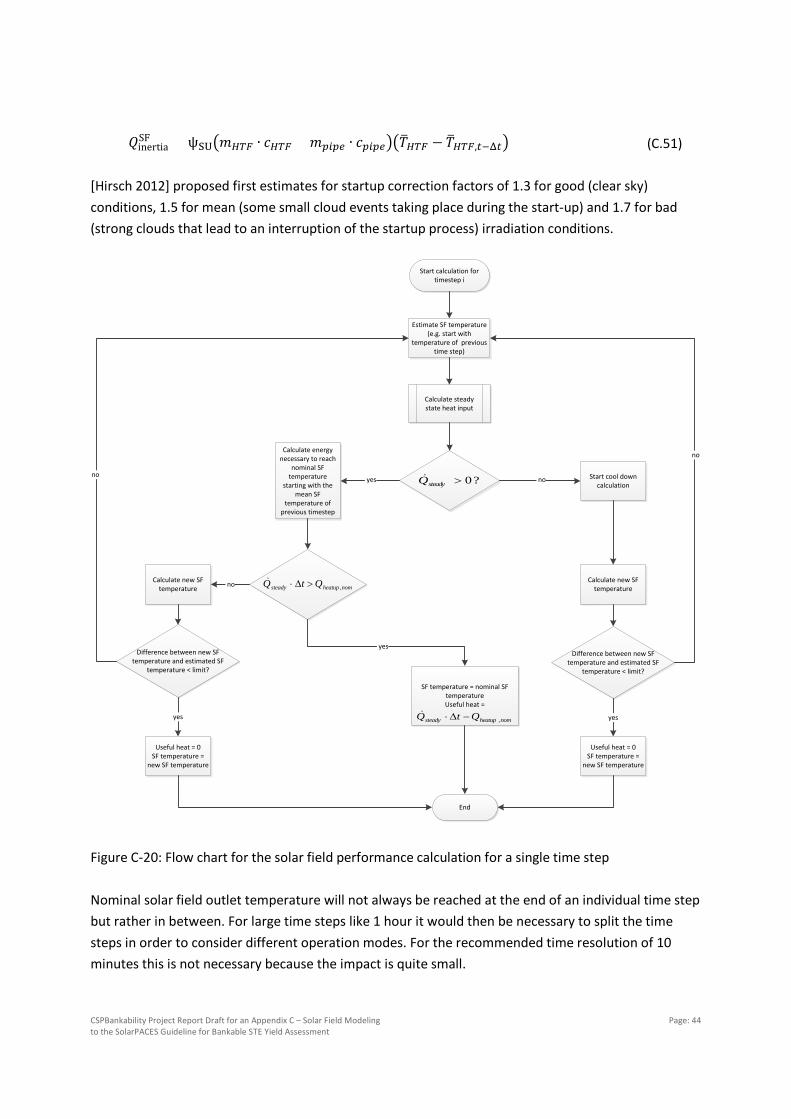
CSPBankability Project Report Draft for an Appendix C – Solar Field Modeling to the SolarPACES Guideline for Bankable STE Yield Assessment
Page: 44
𝑄𝑄inertiaSF = ψSU�𝑚𝑚𝐻𝐻𝐻𝐻𝐻𝐻 ∙ 𝑐𝑐𝐻𝐻𝐻𝐻𝐻𝐻 + 𝑚𝑚𝑜𝑜𝑎𝑎𝑜𝑜𝑠𝑠 ∙ 𝑐𝑐𝑜𝑜𝑎𝑎𝑜𝑜𝑠𝑠��𝑇𝑇�𝐻𝐻𝐻𝐻𝐻𝐻 − 𝑇𝑇�𝐻𝐻𝐻𝐻𝐻𝐻,𝑡𝑡−Δ𝑡𝑡� (C.51)
[Hirsch 2012] proposed first estimates for startup correction factors of 1.3 for good (clear sky) conditions, 1.5 for mean (some small cloud events taking place during the start-up) and 1.7 for bad (strong clouds that lead to an interruption of the startup process) irradiation conditions.
Figure C-20: Flow chart for the solar field performance calculation for a single time step Nominal solar field outlet temperature will not always be reached at the end of an individual time step but rather in between. For large time steps like 1 hour it would then be necessary to split the time steps in order to consider different operation modes. For the recommended time resolution of 10 minutes this is not necessary because the impact is quite small.
Start calculation for timestep i
Calculate steady state heat input
?0>steadyQ Start cool down calculation
no
Calculate energy necessary to reach
nominal SF temperature
starting with the mean SF
temperature of previous timestep
yes
nomheatupsteady QtQ ,>∆⋅
SF temperature = nominal SF temperatureUseful heat =
yes
nomheatupsteady QtQ ,−∆⋅
End
Estimate SF temperature(e.g. start with
temperature of previous time step)
Calculate new SF temperature no
Difference between new SF temperature and estimated SF
temperature < limit?
no
Useful heat = 0SF temperature =
new SF temperature
yes
Calculate new SF temperature
Difference between new SF temperature and estimated SF
temperature < limit?
Useful heat = 0SF temperature =
new SF temperature
yes
no
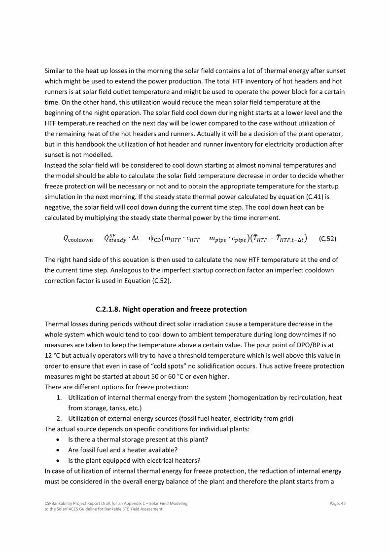
CSPBankability Project Report Draft for an Appendix C – Solar Field Modeling to the SolarPACES Guideline for Bankable STE Yield Assessment
Page: 45
Similar to the heat up losses in the morning the solar field contains a lot of thermal energy after sunset which might be used to extend the power production. The total HTF inventory of hot headers and hot runners is at solar field outlet temperature and might be used to operate the power block for a certain time. On the other hand, this utilization would reduce the mean solar field temperature at the beginning of the night operation. The solar field cool down during night starts at a lower level and the HTF temperature reached on the next day will be lower compared to the case without utilization of the remaining heat of the hot headers and runners. Actually it will be a decision of the plant operator, but in this handbook the utilization of hot header and runner inventory for electricity production after sunset is not modelled. Instead the solar field will be considered to cool down starting at almost nominal temperatures and the model should be able to calculate the solar field temperature decrease in order to decide whether freeze protection will be necessary or not and to obtain the appropriate temperature for the startup simulation in the next morning. If the steady state thermal power calculated by equation (C.41) is negative, the solar field will cool down during the current time step. The cool down heat can be calculated by multiplying the steady state thermal power by the time increment. 𝑄𝑄cooldown = �̇�𝑄𝑡𝑡𝑡𝑡𝑠𝑠𝑡𝑡𝑠𝑠𝑠𝑠𝑆𝑆𝐻𝐻 ∙ Δ𝑡𝑡 = ψCD�𝑚𝑚𝐻𝐻𝐻𝐻𝐻𝐻 ∙ 𝑐𝑐𝐻𝐻𝐻𝐻𝐻𝐻 + 𝑚𝑚𝑜𝑜𝑎𝑎𝑜𝑜𝑠𝑠 ∙ 𝑐𝑐𝑜𝑜𝑎𝑎𝑜𝑜𝑠𝑠��𝑇𝑇�𝐻𝐻𝐻𝐻𝐻𝐻 − 𝑇𝑇�𝐻𝐻𝐻𝐻𝐻𝐻,𝑡𝑡−Δ𝑡𝑡� (C.52) The right hand side of this equation is then used to calculate the new HTF temperature at the end of the current time step. Analogous to the imperfect startup correction factor an imperfect cooldown correction factor is used in Equation (C.52).
C.2.1.8. Night operation and freeze protection
Thermal losses during periods without direct solar irradiation cause a temperature decrease in the whole system which would tend to cool down to ambient temperature during long downtimes if no measures are taken to keep the temperature above a certain value. The pour point of DPO/BP is at 12 °C but actually operators will try to have a threshold temperature which is well above this value in order to ensure that even in case of “cold spots” no solidification occurs. Thus active freeze protection measures might be started at about 50 or 60 °C or even higher. There are different options for freeze protection:
1. Utilization of internal thermal energy from the system (homogenization by recirculation, heat from storage, tanks, etc.)
2. Utilization of external energy sources (fossil fuel heater, electricity from grid) The actual source depends on specific conditions for individual plants:
• Is there a thermal storage present at this plant? • Are fossil fuel and a heater available? • Is the plant equipped with electrical heaters?
In case of utilization of internal thermal energy for freeze protection, the reduction of internal energy must be considered in the overall energy balance of the plant and therefore the plant starts from a
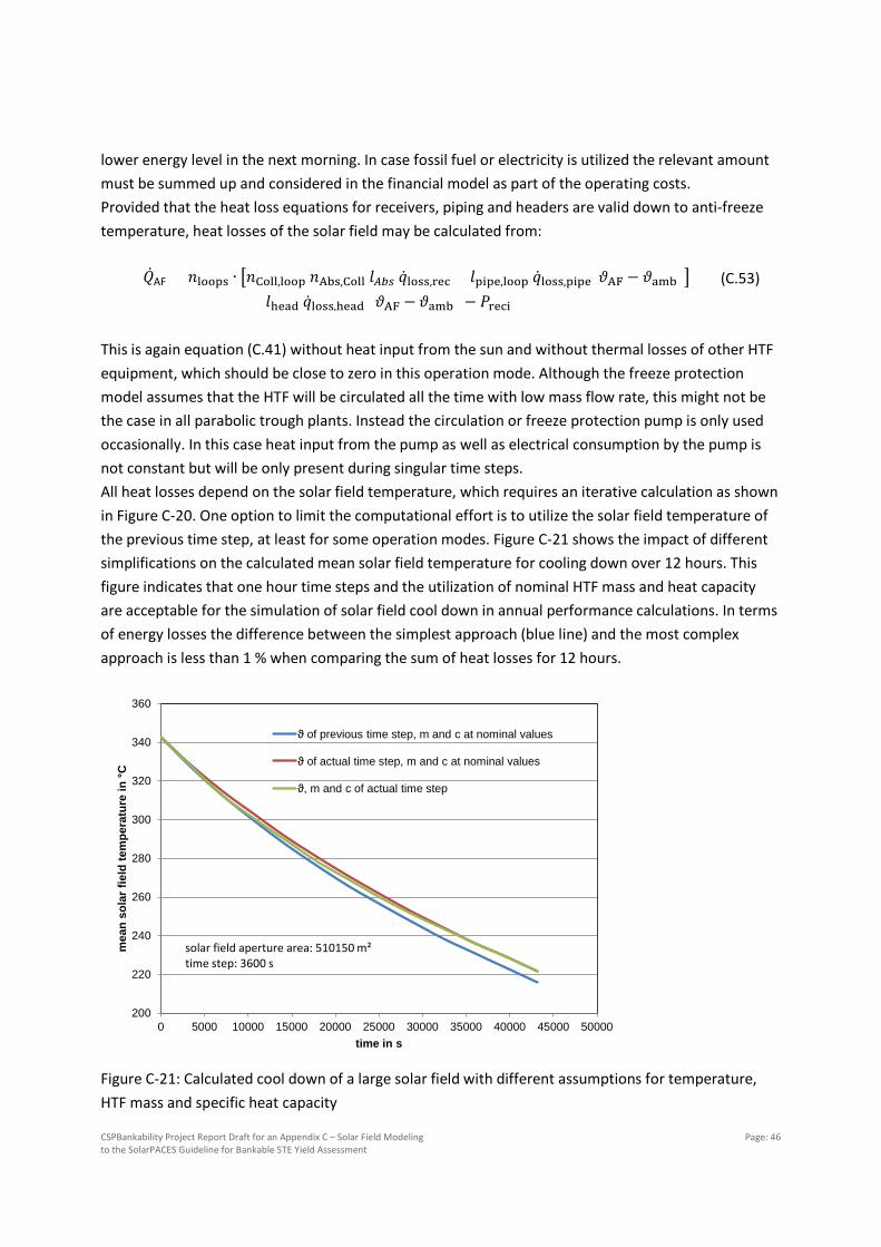
CSPBankability Project Report Draft for an Appendix C – Solar Field Modeling to the SolarPACES Guideline for Bankable STE Yield Assessment
Page: 46
lower energy level in the next morning. In case fossil fuel or electricity is utilized the relevant amount must be summed up and considered in the financial model as part of the operating costs. Provided that the heat loss equations for receivers, piping and headers are valid down to anti-freeze temperature, heat losses of the solar field may be calculated from: �̇�𝑄AF = 𝑛𝑛loops ∙ �𝑛𝑛Coll,loop 𝑛𝑛Abs,Coll 𝑙𝑙𝑓𝑓𝑎𝑎𝑡𝑡 �̇�𝑞loss,rec + 𝑙𝑙pipe,loop �̇�𝑞loss,pipe(𝜗𝜗AF − 𝜗𝜗amb)�
+ 𝑙𝑙head �̇�𝑞loss,head (𝜗𝜗AF − 𝜗𝜗amb) − 𝑃𝑃reci (C.53)
This is again equation (C.41) without heat input from the sun and without thermal losses of other HTF equipment, which should be close to zero in this operation mode. Although the freeze protection model assumes that the HTF will be circulated all the time with low mass flow rate, this might not be the case in all parabolic trough plants. Instead the circulation or freeze protection pump is only used occasionally. In this case heat input from the pump as well as electrical consumption by the pump is not constant but will be only present during singular time steps. All heat losses depend on the solar field temperature, which requires an iterative calculation as shown in Figure C-20. One option to limit the computational effort is to utilize the solar field temperature of the previous time step, at least for some operation modes. Figure C-21 shows the impact of different simplifications on the calculated mean solar field temperature for cooling down over 12 hours. This figure indicates that one hour time steps and the utilization of nominal HTF mass and heat capacity are acceptable for the simulation of solar field cool down in annual performance calculations. In terms of energy losses the difference between the simplest approach (blue line) and the most complex approach is less than 1 % when comparing the sum of heat losses for 12 hours.
Figure C-21: Calculated cool down of a large solar field with different assumptions for temperature, HTF mass and specific heat capacity
200
220
240
260
280
300
320
340
360
0 5000 10000 15000 20000 25000 30000 35000 40000 45000 50000
mea
n so
lar f
ield
tem
pera
ture
in °C
time in s
ϑ of previous time step, m and c at nominal values
ϑ of actual time step, m and c at nominal values
ϑ, m and c of actual time step
solar field aperture area: 510150 m²time step: 3600 s

CSPBankability Project Report Draft for an Appendix C – Solar Field Modeling to the SolarPACES Guideline for Bankable STE Yield Assessment
Page: 47
From Figure C-22 it is obvious that the error becomes smaller when switching to 10 minutes time steps as recommended.
Figure C-22: Calculated cool down of a large solar field with different time steps
C.2.1.9. Interface variables
For the annual performance simulation of the whole CSP plant several interface variables as defined in Appendix A must be calculated. From the solar field’s view point inlet temperature, inlet enthalpy and outlet pressure are input variables. Outlet temperature, outlet enthalpy, inlet pressure, HTF mass flow rate, net thermal power and auxiliary consumption are output variables. For the calculation of output interface variables the current status of the solar field must be determined as shown in Figure C-20. If the solar field can deliver net thermal power the following table is valid: 𝑇𝑇out
SF = 𝑇𝑇nomSF 3 (C.54)
ℎoutSF = ℎnom
SF (C.55)
�̇�𝑄𝑆𝑆𝐻𝐻 from equation (C.41) (C.56)
3 Must not be neccessarily nominal SF outlet temperature. The OS should at least have the option request a SF temperature for the time step and the SF must try to deliver this temperature
200
220
240
260
280
300
320
340
360
0 5000 10000 15000 20000 25000 30000 35000 40000 45000 50000
mea
n so
lar f
ield
tem
pera
ture
in °C
time in s
time step 3600 s time step 600s
solar field aperture area: 510150 m²ϑ of previous time step, m and c at nominal values
CSPBankability Project Report Draft for an Appendix C – Solar Field Modeling to the SolarPACES Guideline for Bankable STE Yield Assessment
Page: 48
�̇�𝑚SF =�̇�𝑄SF
�ℎoutSF − ℎin
SF� (C.57)
p𝑎𝑎𝑡𝑡𝑆𝑆𝐻𝐻 = 𝑝𝑝𝑜𝑜𝑝𝑝𝑡𝑡𝑆𝑆𝐻𝐻 − ∆𝑝𝑝nom �
�̇�𝑚𝐻𝐻𝐻𝐻𝐻𝐻 ∙ 𝜌𝜌𝐻𝐻𝐻𝐻𝐻𝐻,𝑡𝑡𝑜𝑜𝑎𝑎
�̇�𝑚𝐻𝐻𝐻𝐻𝐻𝐻,𝑡𝑡𝑜𝑜𝑎𝑎 ∙ 𝜌𝜌𝐻𝐻𝐻𝐻𝐻𝐻 �2
(C.58)
P𝑡𝑡𝑝𝑝𝑎𝑎𝑆𝑆𝐻𝐻 = 𝑃𝑃pump,nom �
�̇�𝑚𝐻𝐻𝐻𝐻𝐻𝐻 ∙ 𝜌𝜌𝐻𝐻𝐻𝐻𝐻𝐻,𝑡𝑡𝑜𝑜𝑎𝑎
�̇�𝑚𝐻𝐻𝐻𝐻𝐻𝐻,𝑡𝑡𝑜𝑜𝑎𝑎 ∙ 𝜌𝜌𝐻𝐻𝐻𝐻𝐻𝐻 �2
+ 𝑃𝑃𝑓𝑓𝑎𝑎𝑎𝑎,𝑜𝑜𝑡𝑡𝑆𝑆𝐻𝐻
(C.59)
If the solar field cannot deliver net thermal power it is in recirculation mode with: 𝑇𝑇𝑜𝑜𝑝𝑝𝑡𝑡𝑆𝑆𝐻𝐻 = 𝑇𝑇𝑎𝑎𝑡𝑡𝑆𝑆𝐻𝐻 (C.60)
ℎ𝑜𝑜𝑝𝑝𝑡𝑡𝑆𝑆𝐻𝐻 = ℎ𝑎𝑎𝑡𝑡𝑆𝑆𝐻𝐻 (C.61)
�̇�𝑄𝑆𝑆𝐻𝐻 = 0 (C.62)
�̇�𝑚𝑆𝑆𝐻𝐻 = 0 (C.63)
p𝑎𝑎𝑡𝑡𝑆𝑆𝐻𝐻 = 0 (C.64)
𝑃𝑃𝑡𝑡𝑝𝑝𝑎𝑎𝑆𝑆𝐻𝐻 = 𝑃𝑃reci + 𝑃𝑃𝑓𝑓𝑎𝑎𝑎𝑎,𝑜𝑜𝑓𝑓𝑓𝑓𝑆𝑆𝐻𝐻 (C.65)
C.2.1.10. Plausibility checks
The following checks should be done for a model, in order to identify crude errors:
• Are the associated values for optical efficiency and aperture areas (and eventually specific costs) used?
• Is the IAM function (for parabolic troughs) beneath the cosine function (see Figure C-8)? • Is the approximation for receiver thermal losses valid and physically reasonable for the whole
temperature range? • Check the time code used in the meteorological dataset and take care to use the same time in
the model • Check the definition of the time stamp used in the meteorological data file and use
appropriate time to calculate mean sun position for the time instance. • Plot diagrams of typical solar days and analyze course of power generation in order to identify
failures in the system behavior

CSPBankability Project Report Draft for an Appendix C – Solar Field Modeling to the SolarPACES Guideline for Bankable STE Yield Assessment
Page: 49
C.2.2. Parabolic trough field with two-phase heat transfer fluid (place holder)
C.2.3. Linear Fresnel field with single phase heat transfer fluid (place holder)
C.2.4. Linear Fresnel field with two-phase heat transfer fluid (place holder)
C.3. Solar towers
This chapter will be available by beginning of February 2017.

CSPBankability Project Report Draft for an Appendix C – Solar Field Modeling to the SolarPACES Guideline for Bankable STE Yield Assessment
Page: 50
C.4. Symbols
C.4.1. Symbols used in chapter C.2
Symbol Description Unit
𝐴𝐴net Net aperture area m² 𝐴𝐴nom,reduced Reduced nominal aperture area (due to missing mirrors etc.) m²
𝐴𝐴nom∗ Nominal aperture area without receiver area m² 𝐴𝐴nom,loop Nominal aperture area of one loop m²
𝐴𝐴rec Net receiver area m²
𝐴𝐴SF Aperture area of the solar field m²
𝑎𝑎k Coefficient of the IAM equation
𝑎𝑎shad Additional shaded fraction of the solar field -
𝑏𝑏h Factor considering the piping mass and heat capacity in relation to the HTF mass and heat capacity
-
𝑏𝑏i Coefficient of receiver heat loss equation
𝑐𝑐HTF Specific heat capacity of HTF kJ/kg/K 𝑐𝑐pipe Specific heat capacity of pipe material kJ/kg/K
𝑑𝑑col Axial distance between collectors in a row m
𝑑𝑑row Row distance in the solar field m
𝐹𝐹′ Heat loss factor accounting for the difference between absorber temperature and bulk HTF temperature
-
𝑓𝑓 Collector focal length m
𝑓𝑓corr Correction factor to account for the non-linearity of receiver heat losses in temperature
-
𝑓𝑓focA Focusing factor -
𝐺𝐺bn Beam irradiance W/m²
𝐺𝐺d Diffuse irradiance W/m²
𝐺𝐺Pr Projected direct irradiance W/m²
𝐾𝐾 Incidence angle modifier -
𝐾𝐾′ Incidence angle modifier including cosine of incidence angle -
𝑙𝑙col Collector length m 𝑙𝑙𝑓𝑓,𝑡𝑡𝑎𝑎𝑠𝑠𝑡𝑡 Average distance between reflector and receiver m 𝑙𝑙𝑜𝑜𝑎𝑎𝑜𝑜𝑠𝑠 Piping length m
𝑙𝑙𝑜𝑜𝑎𝑎𝑜𝑜𝑠𝑠,𝑎𝑎𝑜𝑜𝑜𝑜𝑜𝑜 Total piping length of one loop (excluding receivers) m
𝑙𝑙head header length m
ℎinSF Inlet enthalpy of SF kJ/kg
ℎoutSF Outlet enthalpy of SF kJ/kg
𝑙𝑙rec Receiver length m

CSPBankability Project Report Draft for an Appendix C – Solar Field Modeling to the SolarPACES Guideline for Bankable STE Yield Assessment
Page: 51
𝑚𝑚HTF Total mass of HTF kg 𝑚𝑚pipe Total mass of pipes (loop piping and headers) kg
�̇�𝑚HTF HTF mass flow rate kg/s 𝑛𝑛𝑓𝑓𝑜𝑜𝑎𝑎,𝑎𝑎𝑜𝑜𝑜𝑜𝑜𝑜 Number of collectors per loop -
𝑛𝑛col,row Number of collectors in one row - 𝑛𝑛𝑡𝑡𝑠𝑠𝑓𝑓,𝑓𝑓𝑜𝑜𝑎𝑎𝑎𝑎 Number of receivers per collector -
𝑛𝑛row Total number of rows in the solar field - 𝑛𝑛row,unshad Number of rows which are not affected by shading -
𝑃𝑃auxSF Total auxiliary power consumption of SF W 𝑃𝑃aux,fixSF Constant auxiliary power consumption of SF W
𝑃𝑃aux,varSF Variable (load dependent) auxiliary power consumption of SF W 𝑃𝑃el,P Electrical power consumption of solar field pumps W 𝑃𝑃𝑠𝑠𝑎𝑎,𝑜𝑜𝑡𝑡𝑆𝑆𝐻𝐻 Total online electric power consumption of solar field W 𝑃𝑃fix,offSF Constant part of the offline electric power consumption of solar
field W
𝑃𝑃fix,onSF Constant part of the online electric power consumption of solar
field W
𝑃𝑃𝑠𝑠𝑎𝑎,𝑜𝑜𝑓𝑓𝑓𝑓𝑆𝑆𝐻𝐻 Total offline electric power consumption of solar field W
𝑃𝑃reci Power consumption of the solar field recirculation pump (pump used for circulating the HTF when the solar field is in start-up or anti-freeze mode)
W
𝑃𝑃pump,nom Nominal power of main HTF pumps W
𝑝𝑝inSF Pressure at SF inlet bar
𝑝𝑝outSF Pressure at SF outlet bar
𝑄𝑄cooldown Cool down heat within a time interval J
𝑄𝑄inertiaSF Heat used for solar field heat up within a time interval J
𝑄𝑄SF Total delivered heat by the solar field within a time interval J
�̇�𝑄AF Anti-freeze thermal power W
�̇�𝑄TH Thermal power from trace heating W
�̇�𝑄abs Absorbed thermal power W �̇�𝑄abs,0 Nominal absorbed thermal power W
�̇�𝑄ext Heat gain from external sources (e.g. solar field pumps or trace heating
W
�̇�𝑄𝑎𝑎𝑜𝑜𝑜𝑜𝑜𝑜,𝑡𝑡𝑡𝑡𝑠𝑠𝑡𝑡𝑠𝑠𝑠𝑠 Thermal power delivered by one loop calculated without considering transient effects
W
�̇�𝑄loss Heat losses W
�̇�𝑄𝑎𝑎𝑜𝑜𝑡𝑡𝑡𝑡,cold ℎ𝑠𝑠𝑡𝑡𝑠𝑠 Heat loss of cold header W �̇�𝑄loss,head Header heat losses W
�̇�𝑄𝑎𝑎𝑜𝑜𝑡𝑡𝑡𝑡,hot ℎ𝑠𝑠𝑡𝑡𝑠𝑠 Heat loss of hot header W

CSPBankability Project Report Draft for an Appendix C – Solar Field Modeling to the SolarPACES Guideline for Bankable STE Yield Assessment
Page: 52
�̇�𝑄loss,loop Total heat loss of a single loop W �̇�𝑄loss,rec Receiver heat losses W �̇�𝑄loss,pipe Piping heat losses of solar field loops W �̇�𝑄pump Heat gain caused by HTF pumps W
�̇�𝑄𝑆𝑆𝐻𝐻 Thermal power delivered by solar field W �̇�𝑄𝑡𝑡𝑡𝑡𝑠𝑠𝑡𝑡𝑠𝑠𝑠𝑠𝑆𝑆𝐻𝐻 Thermal power delivered by solar field calculated without
considering transient effects W
�̇�𝑄∆p Thermal power input to the solar field due to friction losses of the HTF
W
�̇�𝑞loss,corr Corrected specific receiver heat loss W/m �̇�𝑞loss,head Specific header losses based on header length W/m
�̇�𝑞loss,head,A Specific header losses based on net aperture area W/m² �̇�𝑞loss,pipe Specific piping heat losses based on pipe length W/m
�̇�𝑞loss,pipe,nom Specific piping heat losses based on pipe length for nominal solar field conditions
W/m
�̇�𝑞loss,rec Specific receiver heat losses based on receiver length W/m
𝑇𝑇amb Ambient temperature K
𝑇𝑇HTF Bulk HTF temperature K
𝑇𝑇inSF Solar field inlet temperature K
𝑇𝑇loop,in Loop inlet temperature K 𝑇𝑇loop,out Loop outlet temperature K
𝑇𝑇outSF Solar field outlet temperature K
𝑇𝑇pump,in HTF temperature at pump inlet K 𝑇𝑇pump,out HTF temperature at pump outlet K
𝑇𝑇�HTF Local mean HTF temperature of the current time step K
𝑇𝑇�𝐻𝐻𝐻𝐻𝐻𝐻,𝑡𝑡−Δ𝑡𝑡 Local mean HTF temperature of the previous time step K �̇�𝑉HTF,nom Nominal HTF volume flow rate m³/s
𝑣𝑣HTF Velocity of heat transfer fluid m/s
𝑣𝑣wind Wind velocity m/s
𝑤𝑤col Collector aperture width m
Greek symbols
𝛼𝛼S Solar altitude angle °
𝛽𝛽A Collector axis tilt angle °
𝛾𝛾A Collector axis azimuth angle °
𝛾𝛾S Solar azimuth angle °
∆p Pressure loss bar
Δ𝑡𝑡 Time intervall s
𝜂𝜂abs Receiver tube absorptance -

CSPBankability Project Report Draft for an Appendix C – Solar Field Modeling to the SolarPACES Guideline for Bankable STE Yield Assessment
Page: 53
𝜂𝜂atten Atmospheric attenuation efficiency -
𝜂𝜂availSF Solar field availability -
𝜂𝜂block Blocking efficiency -
𝜂𝜂clean Cleanliness factor - 𝜂𝜂phi Incidence angle efficiency including all losses caused by non-
perpendicular sun rays into the aperture plane -
𝜂𝜂endloss End loss efficiency -
𝜂𝜂refclean Reflector cleanliness -
𝜂𝜂inter Intercept factor - 𝜂𝜂opt Optical efficiency - 𝜂𝜂opt,0 Clean optical efficiency at incidence angle of zero -
𝜂𝜂𝑜𝑜𝑜𝑜𝑡𝑡,0,𝑡𝑡𝑜𝑜𝑎𝑎𝑎𝑎𝑠𝑠𝑠𝑠 Optical efficiency under soiled conditions -
𝜂𝜂P Pump efficiency - 𝜂𝜂phi Incidence angle efficiency including all losses caused by non-
perpendicular sun rays into the aperture plane -
𝜂𝜂recclean Receiver cleanliness - 𝜂𝜂refl,0 Clean reflector efficiency -
𝜂𝜂shad Shading efficiency - 𝜂𝜂shad,row Row-to-row shading efficiency -
𝜂𝜂trans Transmission through receiver glass cover -
𝜃𝜃i Incidence angle °
𝜗𝜗abs Absorber temperature °C
𝜗𝜗amb Ambient temperature °C
𝜗𝜗HTF HTF bulk temperature °C
ψCD Correction factor to account for non-ideal cooldown -
ψSU Correction factor to account for non-ideal startup -
𝜌𝜌HTF Density of heat transfer fluid kg/m³
𝜌𝜌track Collector track angle °
𝜉𝜉cloud Factor to account for reduced SF output due to transients caused by clouds
-
Subscripts, Superscripts, Abreviations
BP Biphenyl
DPO Diphenyl oxide
HTF Heat transfer fluid
nom nominal
SF Solar field

CSPBankability Project Report Draft for an Appendix C – Solar Field Modeling to the SolarPACES Guideline for Bankable STE Yield Assessment
Page: 54
C.5. References
[Burkholder 2009] F. Burkholder and C. Kutscher: Heat Loss Testing of Schott's 2008 PTR70
Parabolic Trough Receiver, Technical Report NREL/TP-550-45633, May 2009 [Dersch 2012] J. Dersch J, K. Hennecke, V. Quaschning : Free Greenius – New Options and
Availability, Proceedings of the SolarPACES 2012 Conference, 11.-14. September 2012, Marrakech, Morocco
[Duffie 1991] J.A. Duffie, W.A. Beckman: Solar Engineering of Thermal Processes, 2nd ed.,
John Wiley & Sons, New York, 1991 [Forristall 2003] R. Forristall, Heat Transfer Analysis and Modeling of a Parabolic Trough
Solar Receiver Implemented in Engineering Equation Solver, National Renewable Energy Laboratory Technical Report, NREL/TP-550-34169, 2003. Available electronically from http://www.nrel.gov/csp/troughnet/pdfs/34169.pdf
[Herrmann 2004] Herrmann U., Graeter F., Nava P. “Performance of the SKAL-ET collector
loop at KJC Operating Company” SolarPaces Symposium, Mexico, October 6-8, 2004
[Hirsch 2012] Hirsch T., Feldhoff F., Schenk H.: Start-Up Modeling for Annual CSP Yield
Calculations. Journal of Solar Energy Engineering, Vol. 134, August 2012 [Janotte 2012] Janotte, Nicole: Requirements for Representative Acceptance Tests for the
Prediction of the Annual Yield of Parabolic Trough Solar Fields. Dissertation, RWTH Aachen, 2012
[Lüpfert 2004] E. Lüpfert, U. Herrmann, H. Price, E. Zarza, R. Kistner: Towards standard
performance analysis for parabolic trough collector fields. SolarPaces Symposium, Mexico, October 6-8, 2004
[Pernpeintner 2012] J. Pernpeintner: Measurement of Parabolic Trough Receiver Thermal Loss
Power and Relative Optical Efficiency under Solar Simulator Light, Test Report DLR QUARZ, 2012, Available electronically from http://www.dlr.de/sf/Portaldata/73/Resources/dokumente/qualifizierung/quarz/testberichte/DLR-Quarz-Receiver-1207_Schott_R3.pdf

CSPBankability Project Report Draft for an Appendix C – Solar Field Modeling to the SolarPACES Guideline for Bankable STE Yield Assessment
Page: 55
[Riffelmann 2011] K.J. Riffelmann, D. Graf, P. Nava: Suitable Solar Filed Layouts for the Ultimate Trough® Collector SolarPaces Symposium, Granada, Spain, 20.-23. Sept. 2011
[Riffelmann 2014] K.J. Riffelmann, T. Richert, P. Nava. A. Schweitzer: Ultimate Trough® – A
significant step towards cost-competitive CSP. Energy Procedia 49 , pp.1831 – 1839, 2014
[Stine 1985] W.B. Stine and R.W. Harrigan: Solar energy fundamentals and design: with
computer applications. New York, John Wiley & Sons, ISSN 0735-8210, 1985.
[Wilbert 2014] S. Wilbert: Determination of Circumsolar Radiation and its Effect on
Concentrating Solar Power, Dissertation RWTH Aachen, Germany, 2014 [Wittmann 2012] M. Wittmann, F. Feldhoff, T. Hirsch: Determination of Correction Factors
for Heat Losses at High Temperatures in Parabolic Trough Fields. International SolarPaces Conference, Marrakech, Morocco , September 11-14, 2012
Related Documents