DRAFT AGENDA AS OF 09/09/09 - Tucson · Formal Evaluation of Active Managers ... March 2016 Summary Performance Report ... Alliance S&P Index 83,139,473 11.71% 475 5,247,538 77,891,461

TUCSON SUPPLEMENTAL RETIREMENT SYSTEM

BOARD OF TRUSTEES Notice of Regular Meeting / Agenda

DATE: Thursday, April 28, 2016 TIME: 8:30 a.m. PLACE: Finance Department Conference Room, 5th floor

City Hall, 255 West Alameda Tucson, Arizona 85701

A. Consent Agenda

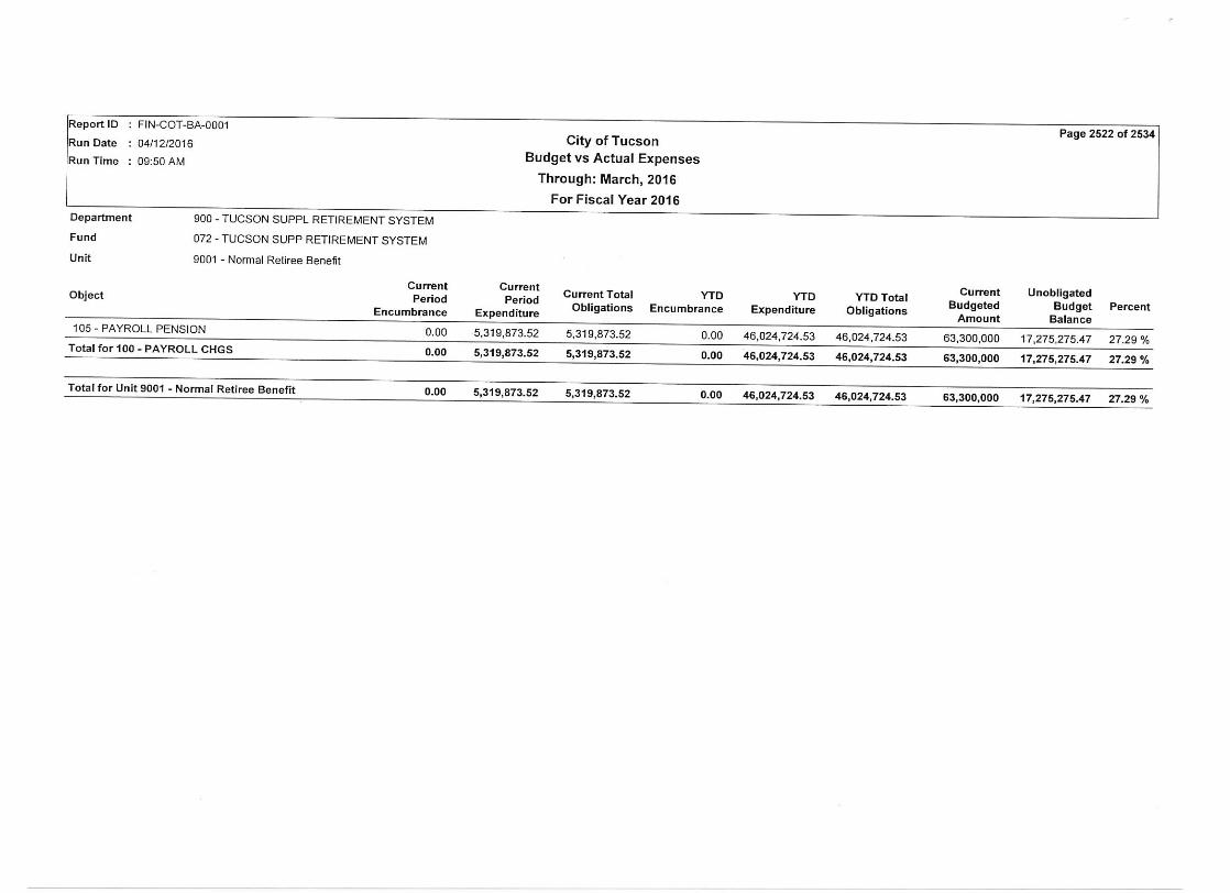
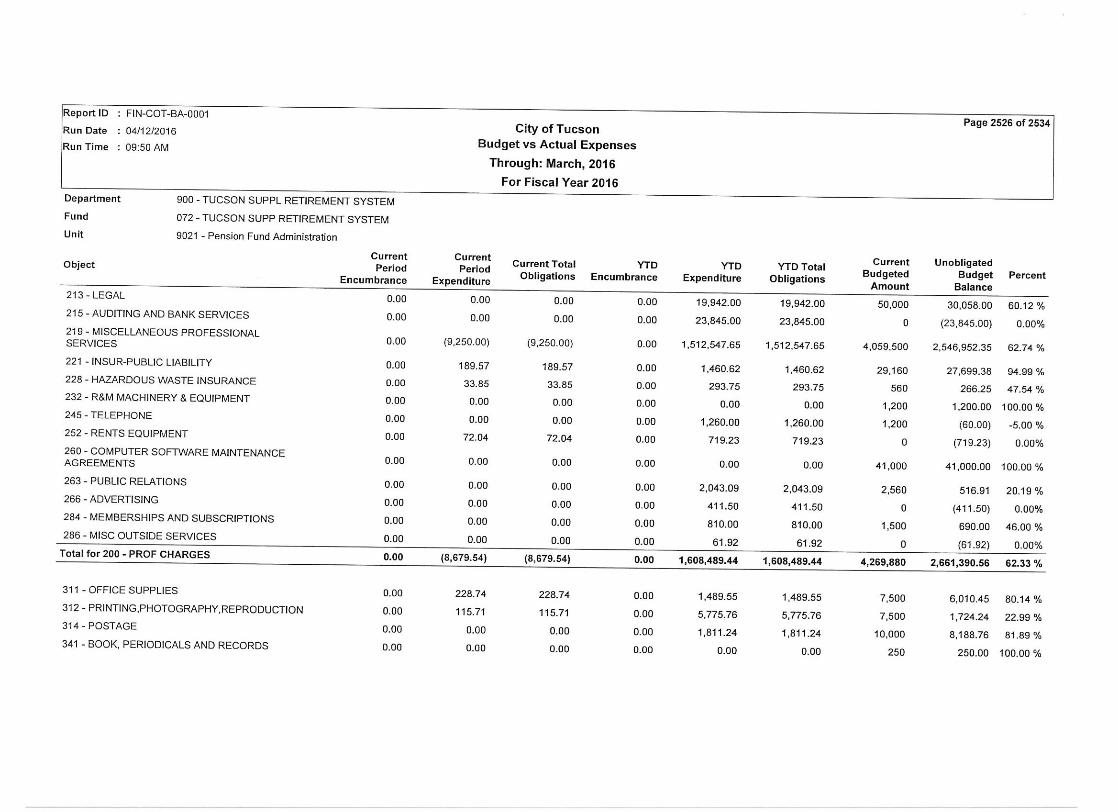
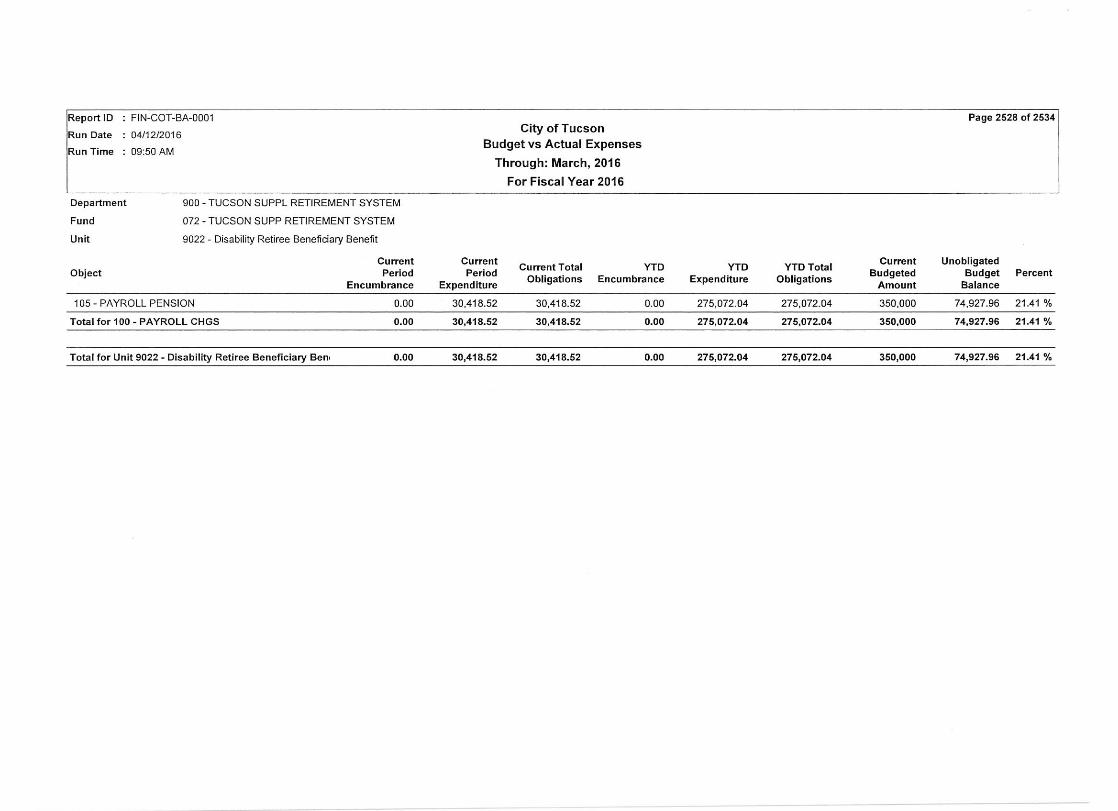
1. Approval of March 31st, 2016 TSRS Board Meeting Minutes 2. Retirement ratifications for April 2016 3. March 2016 TSRS Budget Vs Actual Expenses

B. Disability Applications *

1. Robyn A. Scott 2. Frank Yslas 3. Stephen J. Arnoldi 4. Gilberto Robles

C. Investment Activity Report

1. TSRS Portfolio Composition, Transactions and Performance Review for 03/31/2016 2. Review and Approval of New Portfolio Composition, Transaction, and Performance Reports

D. Administrative Discussions

1. Report from Board Member on 2015 Fall Public Funds Forum 2. 50/50 Split Employee/Employer Contributions for New Hires 3. Volkswagen Securities Litigation Update

E. Articles for Board Member Education / Discussion

1. Causeway Analysis -The Value Reversion

F. Call to Audience

G. Future Agenda Items 1. Education Plan for New Staff and Trustees 2. Duties and Selection of Advisory Board 3. Hiring an Intern to Free Staff for Education 4. TSRS Board Annual Evaluation of Staff and Consultants 5. Formal Evaluation of Active Managers – 1.5% over benchmark over a given period 6. RFQ for Actuarial Services 7. Action Plan for Black Swan Events 8. Would It Be Better to Index the Whole Fund

H. Adjournment

Please Note: Legal Action may be taken on any agenda item *Pursuant to ARS 38-431.03(A)(3) and (4): the board may hold an executive session for the purposes of obtaining legal advice from an attorney or attorneys for the Board or to consider its position and instruct its attorney(s) in pending or contemplated litigation. The board may also hold an executive session pursuant to A.R.S. 38-431.03(A)(2) for purposes of discussion or consideration of records, information or testimony exempt by law from public inspection.

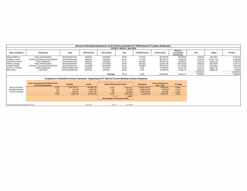
Alberto Robles Jr. Parks and Recreation Normal Retirement 4/2/2016 5/26/1956 59.85 27.6700 294,938.96 96,329.83 3,610.54 J&S 50% 2,129.44Cynthia A. Frank Housing & Community Development Normal Retirement 4/8/2016 4/6/1954 62.01 17.7700 287,342.97 91,549.94 5,429.23 5 Year Term 2,156.85Christine M. Rincon Police Depatment Normal Retirement 4/8/2016 1/19/1955 61.22 18.7900 180,093.29 65,285.51 3,170.13 Single Life 1,339.92Philip E. Damgar Parks and Recreation Normal Retirement 4/2/2016 11/23/1959 56.36 26.5300 323,921.68 105,313.59 3,906.15 J&S 100% 2,146.71Kenneth Snyder Housing & Community Development Normal Retirement 3/12/2016 12/23/1961 54.22 25.8500 353,817.07 111,174.65 4,274.16 J&S 100% 2,322.49Joanne L. Peacher Library Department Deferred Retirement 4/7/2016 3/7/1954 62.08 9.93 62,554.66 33,477.48 2,115.12 Single Life 472.61Ruth Gavin City Courts Deferred Retirement 4/4/2016 4/4/1954 62.00 8.78 83,786.53 24,282.07 3,203.41 Single Life 633.02

25,708.74 11,201.04Averages 26.11 19.33 226,636.45 75,344.72 3,672.68 1,600.15

Plan Year beginning 07/01/2015 (*fromGRS annual valuation) Monthly Annual Annualized Annual change since

July 1, 2015 % change

Service Pensions 2,305 5,007,097.17 60,085,166 2,425 5,304,301 63,651,615.12 3,566,449 5.94%Disability Pensions 160 174,259 2,091,109 150 167,099 2,005,190.64 (85,918) -4.11%Survivor Pensions 344 298,979 3,587,750 338 328,630 3,943,558.08 355,808 9.92%

2,809 5,480,335 65,764,025 2,913 5,800,030 69,600,364 3,836,339 5.83%2 22,097$

S:\treasdiv\tsrs\retirement\facts&figures\F&F 15-16.xls prior month 2,911 5,777,933.08$

Service & Disability Retirements, End of Service Entrants for TSRS Board of Trustees Ratification03/10/16 - 04/09/16 - April 2016

Name of Applicant Department Type Effective Date Date of Birth Age Credited Service Present Value Member's

AccumulatedContributions

AFC Option Pension

Comparison of Monthly Pension Payments - Beginning of FY 2016 to Current Monthly Pension Payments

March 2016 Pension Payroll

(net) change from previous month

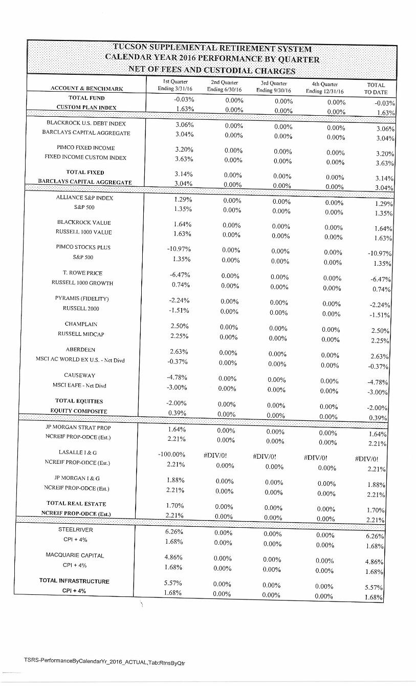
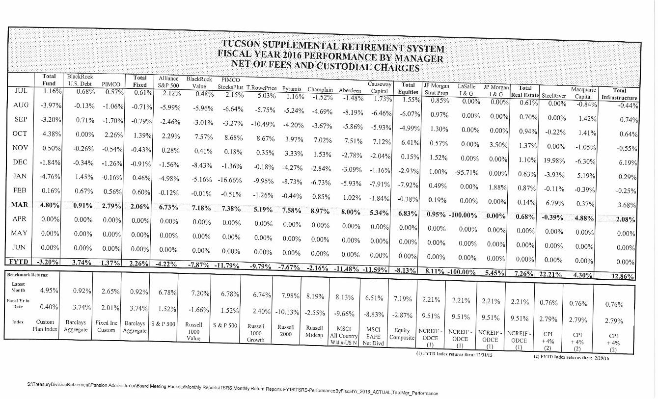
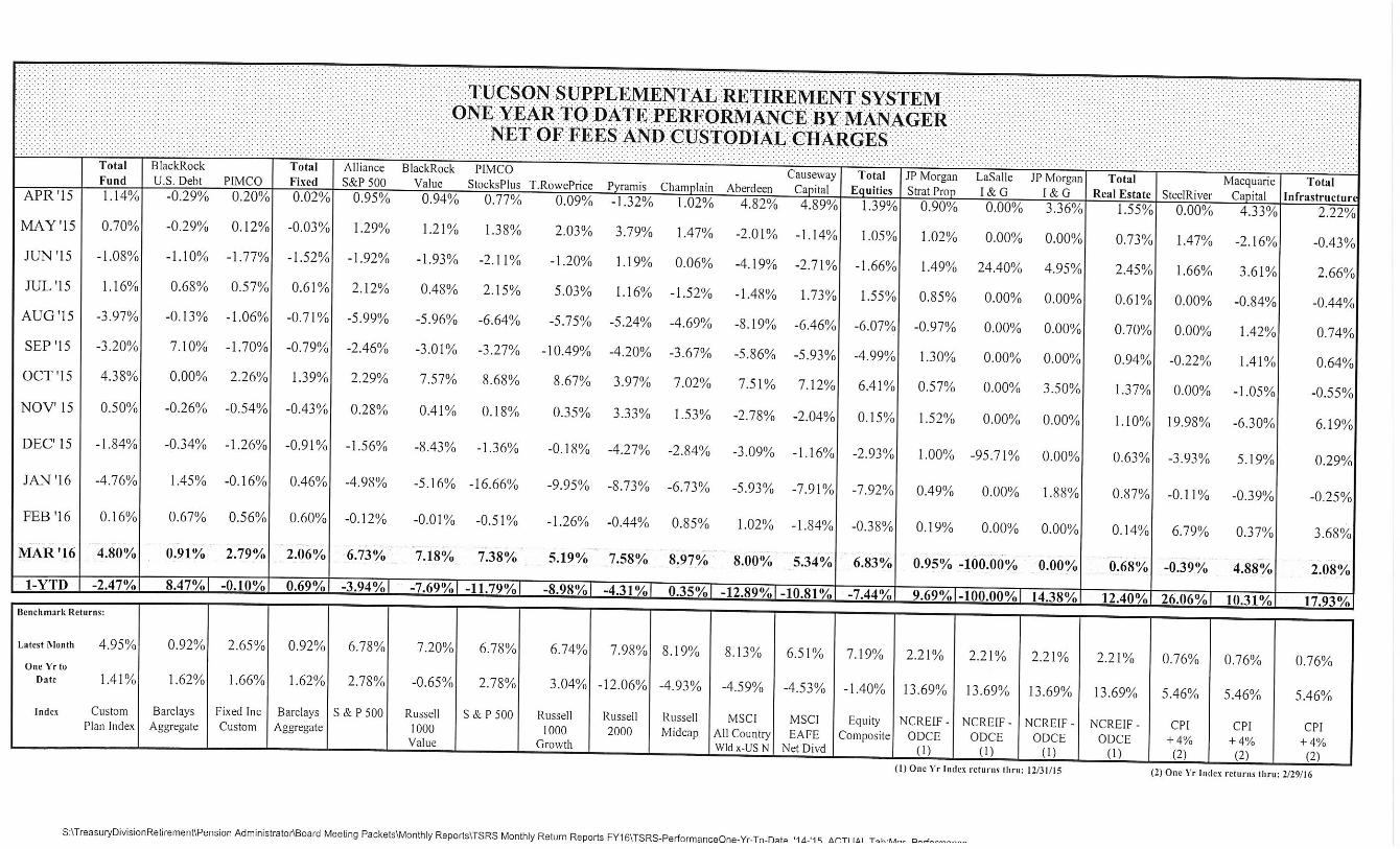
DATE: April 22, 2016 TO: The Board of Trustees Tucson Supplemental Retirement System FROM: Neil S. Galassi, CPA Pension Administrator SUBJECT: March 2016 Summary Performance Report SUMMARY: This report presents the Tucson Supplemental Retirement System’s investment portfolio as of March 31, 2016. Attached to this summary are the detailed reports which the Board has been accustomed to reviewing at monthly Board meetings. As of February 29, 2016 and March 31, 2016, the Total Fund balance was $677.4 million and $709.9 million, respectively. This represents a $42.5 million increase from the prior month. There were no withdrawals from the Total Fund to support pension payments totaled during the recent month, and $22 million has been withdrawn during fiscal year 2016. For the month of March, the Total Fund performance was a positive 4.80% which was slightly worse than the custom benchmark return of positive 4.86% by 6 basis points. Total Fund performance was impacted by large increases in all three of the equity markets; the S&P 500 Index rose 6.65% during the month. For the last twelve months the Total Fund performance was a negative .43% which was behind the custom benchmark of .59%. The Total Fund performance was impacted by large increases for asset balances in the equity markets with the large Cap Equity showing a negative .51%, the Small/Mid Cap Equity showing a negative 1.94%, and the International Equity coming in at negative 11.66%. These returns were all significantly more positive than the month of February 2016. The equity market returns appear consistent with the benchmarks for the same 12 month period with the exception of Small/Mid Cap Equity which outperformed the benchmark by 5.37%. The negative equity returns were somewhat counterbalanced by 12 month positive return on the Real Estate and infrastructure of 11.52% and 10.44% respectively. In regards to equity funds over the past 12 month period, the Small/Mid Cap Equity funds for Champlain Mid Cap and Pyramis Small Cap performed well above their benchmark by 4.39% and 5.39% respectively while the Large Cap Equity fund managers were relatively consistent with their benchmark. The international equity funds of Causeway and Aberdeen trailed their benchmark by 2.48% and 3.70% respectively. For fixed income funds, the PIMCO Fixed Income Fund underperformed the benchmark by 2.80%, while the Barclay’s U.S. Debt Fund was consistent with the benchmark. For Real Estate fund managers, the JPM Strategic Property Fund and he JPM Income and Growth Funds trailed the benchmark by 3.12% and 4.30%. The Macquarie European Infrastructure Fund was 5.86% above the benchmark, and the Steel River Infrastructure fund also outperformed the benchmark by 5.51%.

TSRS Portfolio Performance Review

The Total Fund total as of today, April 22, 2016 was $718.5 million. This represents an increase of $8.6 million (1.20%), over the balance as of March 31, 2016. The increase was primarily a result of a 1.6% increase in asset balances for all equity asset classes. Summary graphs are as follows: . Calendar Year Metrics:

Fiscal Year Metrics:

One Year to Date Performance Metrics:

March 31, 2016

Tucson Supplemental

Retirement System

Investment Measurement ServiceMonthly Review

The following report was prepared by Callan Associates Inc. ("CAI") using information from sources that include the following: fund trustee(s); fundcustodian(s); investment manager(s); CAI computer software; CAI investment manager and fund sponsor database; third party data vendors; and other outsidesources as directed by the client. CAI assumes no responsibility for the accuracy or completeness of the information provided, or methodologies employed, byany information providers external to CAI. Reasonable care has been taken to assure the accuracy of the CAI database and computer software. Callan doesnot provide advice regarding, nor shall Callan be responsible for, the purchase, sale, hedge or holding of individual securities, including, without limitationsecurities of the client (i.e., company stock) or derivatives in the client’s accounts. In preparing the following report, CAI has not reviewed the risks of individualsecurity holdings or the conformity of individual security holdings with the client’s investment policies and guidelines, nor has it assumed any responsibility to doso. Advice pertaining to the merits of individual securities and derivatives should be discussed with a third party securities expert. Copyright 2016 by CallanAssociates Inc.

Table of ContentsTucson Supplemental Retirement SystemMarch 31, 2016

Actual vs. Target Asset Allocation 1

Asset Allocation Across Investment Managers 2

Investment Manager Performance 3

Investment Manager Performance 5

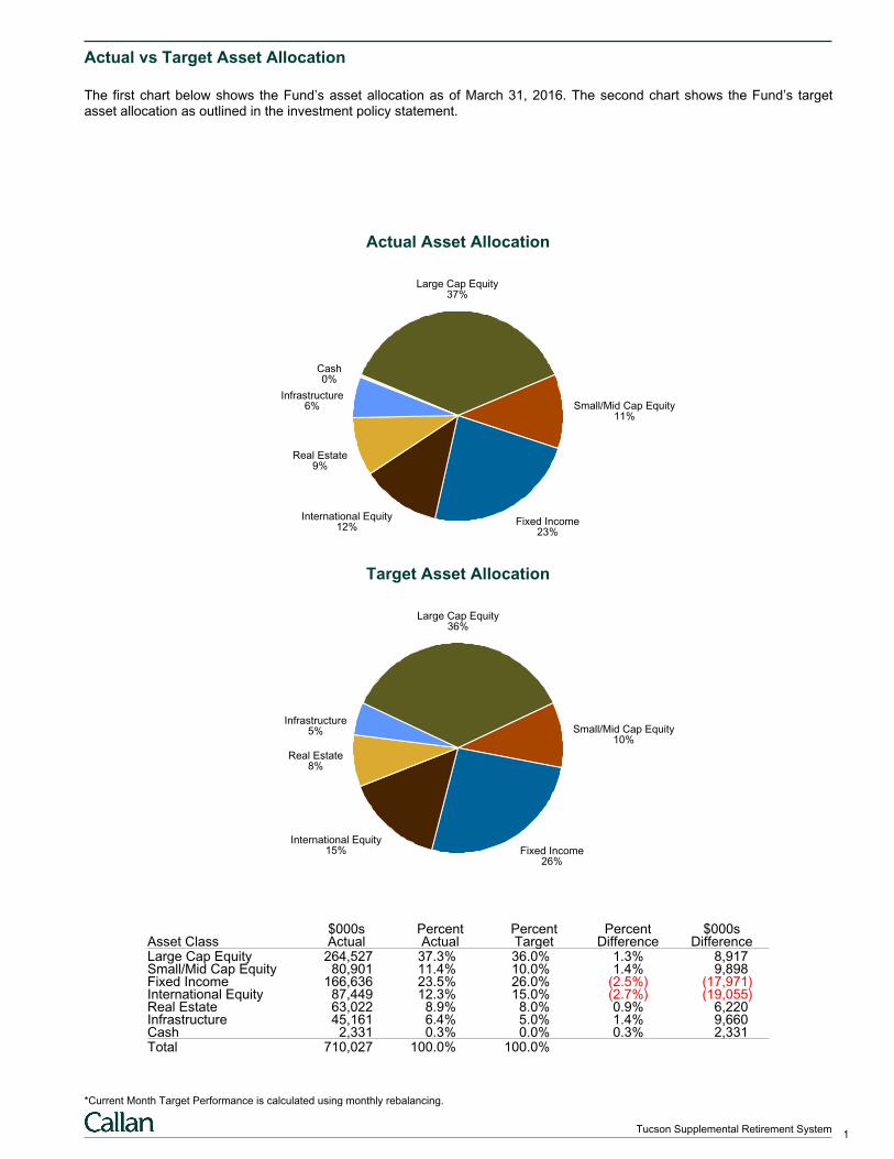
Actual vs Target Asset Allocation

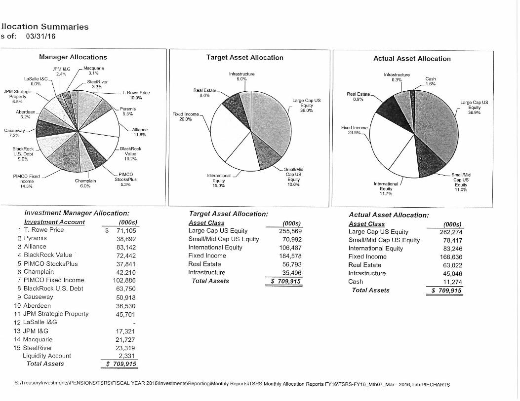
The first chart below shows the Fund’s asset allocation as of March 31, 2016. The second chart shows the Fund’s targetasset allocation as outlined in the investment policy statement.

Actual Asset Allocation

Large Cap Equity37%

Small/Mid Cap Equity11%

Fixed Income23%

International Equity12%

Real Estate9%

Infrastructure6%

Cash0%

Target Asset Allocation

Large Cap Equity36%

Small/Mid Cap Equity10%

Fixed Income26%

International Equity15%

Real Estate8%

Infrastructure5%

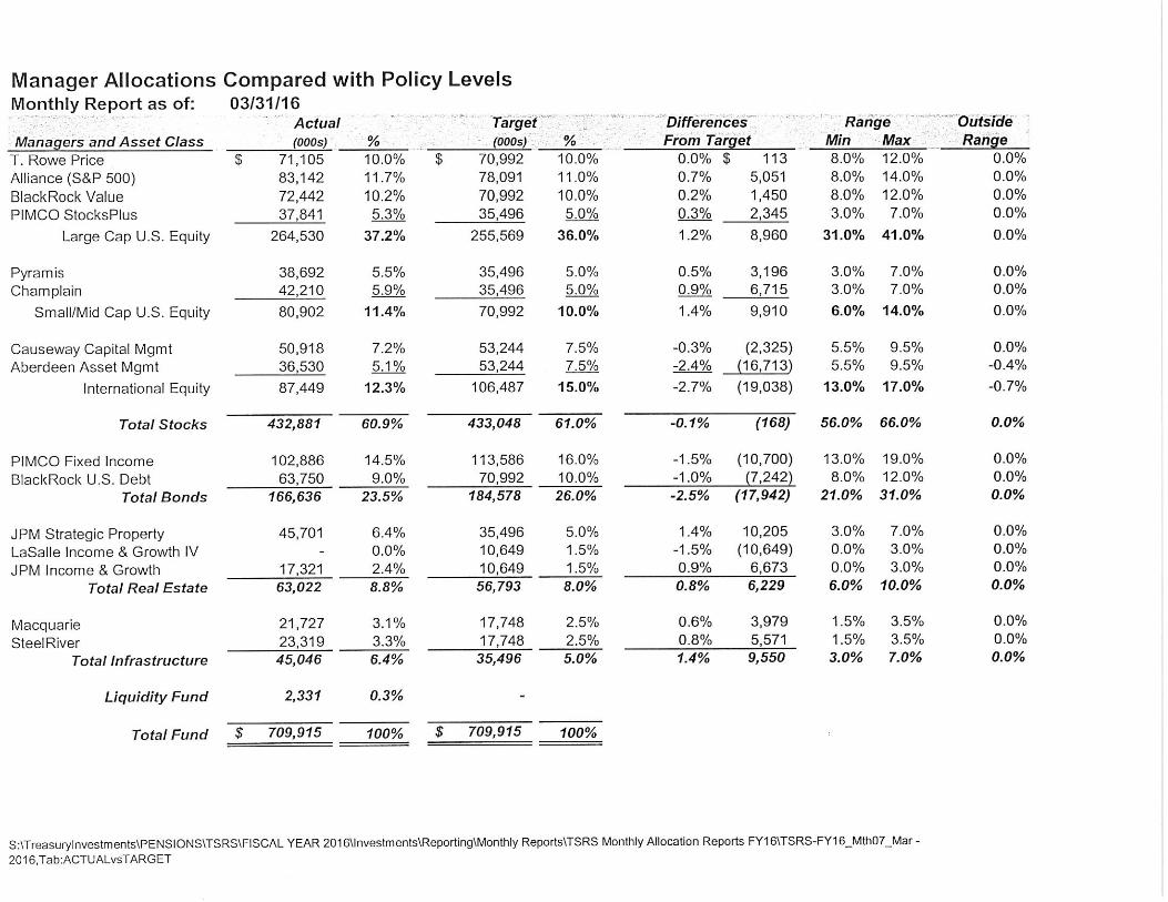
$000s Percent Percent Percent $000sAsset Class Actual Actual Target Difference DifferenceLarge Cap Equity 264,527 37.3% 36.0% 1.3% 8,917Small/Mid Cap Equity 80,901 11.4% 10.0% 1.4% 9,898Fixed Income 166,636 23.5% 26.0% (2.5%) (17,971)International Equity 87,449 12.3% 15.0% (2.7%) (19,055)Real Estate 63,022 8.9% 8.0% 0.9% 6,220Infrastructure 45,161 6.4% 5.0% 1.4% 9,660Cash 2,331 0.3% 0.0% 0.3% 2,331Total 710,027 100.0% 100.0%

*Current Month Target Performance is calculated using monthly rebalancing.

1Tucson Supplemental Retirement System

Investment Manager Asset Allocation

The table below contrasts the distribution of assets across the Fund’s investment managers as of March 31, 2016, with thedistribution as of February 29, 2016. The change in asset distribution is broken down into the dollar change due to Net NewInvestment and the dollar change due to Investment Return.

Asset Distribution Across Investment Managers

March 31, 2016 February 29, 2016

Market Value Percent Net New Inv. Inv. Return Market Value Percent

Domestic Equity $345,427,916 48.65% $(2,303) $22,409,502 $323,020,717 47.68%

Large Cap Equity $264,527,088 37.26% $(5,251) $16,213,441 $248,318,899 36.66%Alliance S&P Index 83,139,473 11.71% 475 5,247,538 77,891,461 11.50%PIMCO StocksPLUS 37,841,114 5.33% 0 2,601,303 35,239,811 5.20%BlackRock Russell 1000 Value 72,441,932 10.20% (7,387) 4,858,595 67,590,724 9.98%T. Rowe Price Large Cap Growth 71,104,569 10.01% 1,661 3,506,006 67,596,903 9.98%

Small/Mid Cap Equity $80,900,828 11.39% $2,948 $6,196,061 $74,701,818 11.03%Champlain Mid Cap 42,210,368 5.94% 1,195 3,473,018 38,736,155 5.72%Pyramis Small Cap 38,690,460 5.45% 1,753 2,723,044 35,965,663 5.31%

International Equity $87,448,834 12.32% $(68,802) $5,356,473 $82,161,164 12.13%Causeway International Value Eq 50,918,483 7.17% 468 2,580,684 48,337,330 7.14%Aberdeen EAFE Plus 36,530,351 5.14% (69,271) 2,775,789 33,823,833 4.99%

Fixed Income $166,635,889 23.47% $(7,623) $3,375,180 $163,268,332 24.10%BlackRock U.S. Debt Fund 63,749,833 8.98% (8,532) 583,019 63,175,346 9.33%PIMCO Fixed Income 102,886,056 14.49% 909 2,792,161 100,092,986 14.78%

Real Estate $63,022,151 8.88% $0 $429,274 $62,592,877 9.24%JPM Strategic Property Fund 45,700,763 6.44% 0 429,274 45,271,489 6.68%JPM Income and Growth Fund 17,321,388 2.44% 0 0 17,321,388 2.56%

Infrastructure $45,161,490 6.36% $0 $1,010,506 $44,150,984 6.52%Macquarie European 21,726,832 3.06% 0 1,010,506 20,716,326 3.06%SteelRiver Infrastructure 23,434,658 3.30% 0 0 23,434,658 3.46%

Total Cash $2,330,534 0.33% $87,907 $443 $2,242,184 0.33%Cash 2,330,534 0.33% 87,907 443 2,242,184 0.33%

Total Fund $710,026,815 100.0% $9,179 $32,581,378 $677,436,258 100.0%


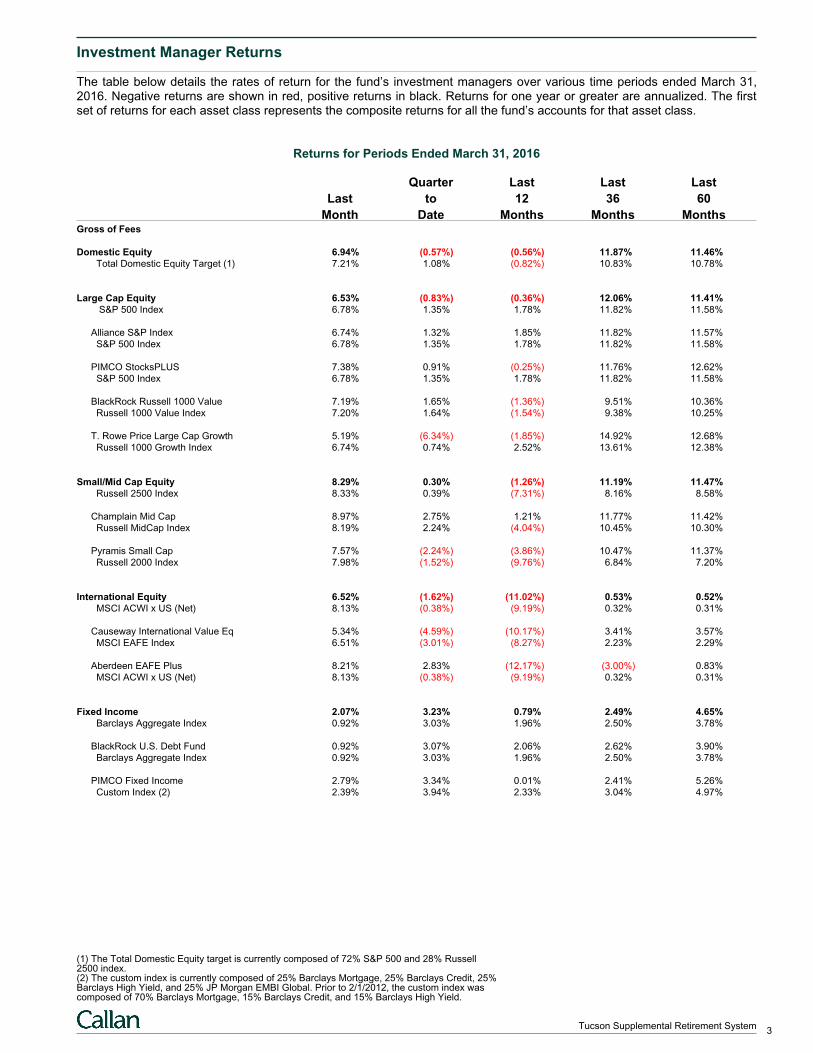
Investment Manager Returns

The table below details the rates of return for the fund’s investment managers over various time periods ended March 31,2016. Negative returns are shown in red, positive returns in black. Returns for one year or greater are annualized. The firstset of returns for each asset class represents the composite returns for all the fund’s accounts for that asset class.

Returns for Periods Ended March 31, 2016

Quarter Last Last Last

Last to 12 36 60

Month Date Months Months MonthsGross of Fees

Domestic Equity 6.94% (0.57%) (0.56%) 11.87% 11.46% Total Domestic Equity Target (1) 7.21% 1.08% (0.82%) 10.83% 10.78%

Large Cap Equity 6.53% (0.83%) (0.36%) 12.06% 11.41% S&P 500 Index 6.78% 1.35% 1.78% 11.82% 11.58%

Alliance S&P Index 6.74% 1.32% 1.85% 11.82% 11.57% S&P 500 Index 6.78% 1.35% 1.78% 11.82% 11.58%

PIMCO StocksPLUS 7.38% 0.91% (0.25%) 11.76% 12.62% S&P 500 Index 6.78% 1.35% 1.78% 11.82% 11.58%

BlackRock Russell 1000 Value 7.19% 1.65% (1.36%) 9.51% 10.36% Russell 1000 Value Index 7.20% 1.64% (1.54%) 9.38% 10.25%

T. Rowe Price Large Cap Growth 5.19% (6.34%) (1.85%) 14.92% 12.68% Russell 1000 Growth Index 6.74% 0.74% 2.52% 13.61% 12.38%

Small/Mid Cap Equity 8.29% 0.30% (1.26%) 11.19% 11.47% Russell 2500 Index 8.33% 0.39% (7.31%) 8.16% 8.58%

Champlain Mid Cap 8.97% 2.75% 1.21% 11.77% 11.42% Russell MidCap Index 8.19% 2.24% (4.04%) 10.45% 10.30%

Pyramis Small Cap 7.57% (2.24%) (3.86%) 10.47% 11.37% Russell 2000 Index 7.98% (1.52%) (9.76%) 6.84% 7.20%

International Equity 6.52% (1.62%) (11.02%) 0.53% 0.52% MSCI ACWI x US (Net) 8.13% (0.38%) (9.19%) 0.32% 0.31%

Causeway International Value Eq 5.34% (4.59%) (10.17%) 3.41% 3.57% MSCI EAFE Index 6.51% (3.01%) (8.27%) 2.23% 2.29%

Aberdeen EAFE Plus 8.21% 2.83% (12.17%) (3.00%) 0.83% MSCI ACWI x US (Net) 8.13% (0.38%) (9.19%) 0.32% 0.31%

Fixed Income 2.07% 3.23% 0.79% 2.49% 4.65% Barclays Aggregate Index 0.92% 3.03% 1.96% 2.50% 3.78%

BlackRock U.S. Debt Fund 0.92% 3.07% 2.06% 2.62% 3.90% Barclays Aggregate Index 0.92% 3.03% 1.96% 2.50% 3.78%

PIMCO Fixed Income 2.79% 3.34% 0.01% 2.41% 5.26% Custom Index (2) 2.39% 3.94% 2.33% 3.04% 4.97%

(1) The Total Domestic Equity target is currently composed of 72% S&P 500 and 28% Russell2500 index.(2) The custom index is currently composed of 25% Barclays Mortgage, 25% Barclays Credit, 25%Barclays High Yield, and 25% JP Morgan EMBI Global. Prior to 2/1/2012, the custom index wascomposed of 70% Barclays Mortgage, 15% Barclays Credit, and 15% Barclays High Yield.






Last to 12 36 60

Month Date Months Months Months

Gross of Fees

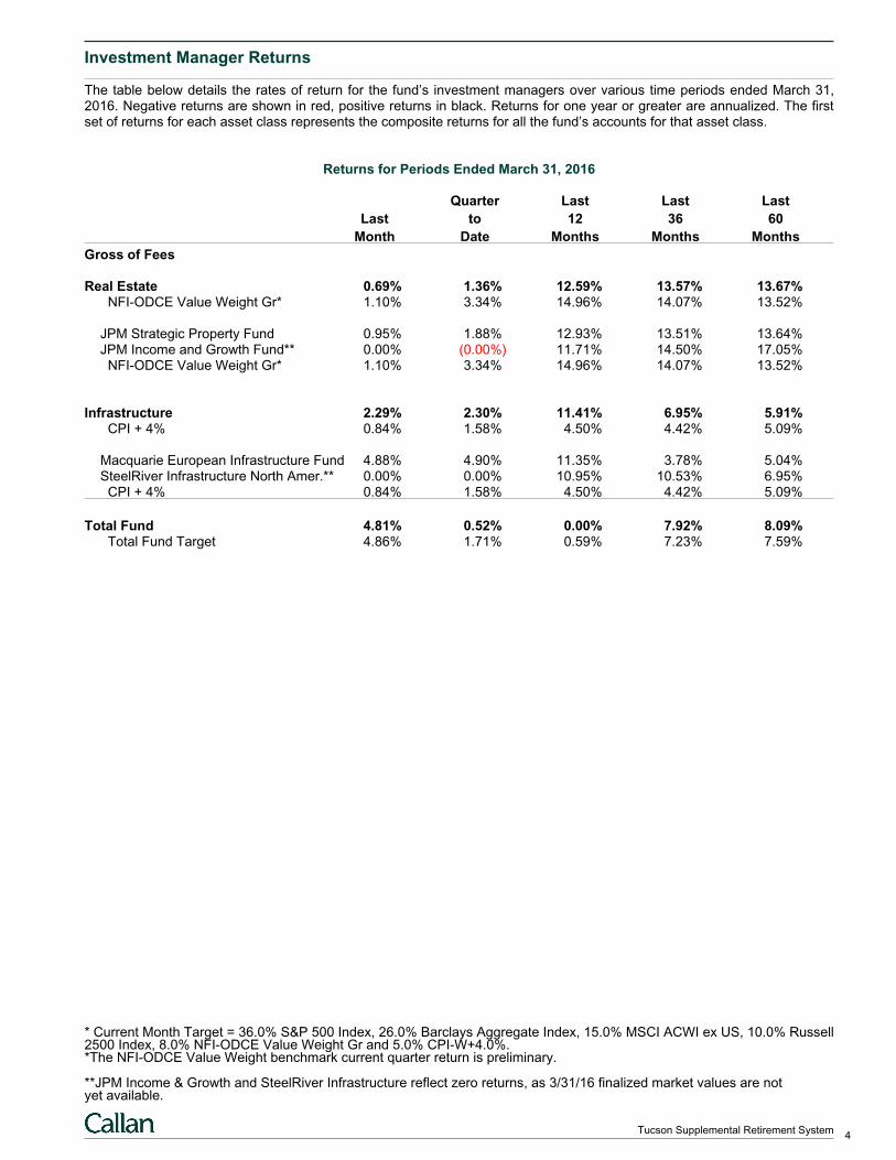
Real Estate 0.69% 1.36% 12.59% 13.57% 13.67% NFI-ODCE Value Weight Gr* 1.10% 3.34% 14.96% 14.07% 13.52%

JPM Strategic Property Fund 0.95% 1.88% 12.93% 13.51% 13.64%JPM Income and Growth Fund** 0.00% (0.00%) 11.71% 14.50% 17.05% NFI-ODCE Value Weight Gr* 1.10% 3.34% 14.96% 14.07% 13.52%

Infrastructure 2.29% 2.30% 11.41% 6.95% 5.91% CPI + 4% 0.84% 1.58% 4.50% 4.42% 5.09%

Macquarie European Infrastructure Fund 4.88% 4.90% 11.35% 3.78% 5.04%SteelRiver Infrastructure North Amer.** 0.00% 0.00% 10.95% 10.53% 6.95% CPI + 4% 0.84% 1.58% 4.50% 4.42% 5.09%

Total Fund 4.81% 0.52% 0.00% 7.92% 8.09% Total Fund Target 4.86% 1.71% 0.59% 7.23% 7.59%

* Current Month Target = 36.0% S&P 500 Index, 26.0% Barclays Aggregate Index, 15.0% MSCI ACWI ex US, 10.0% Russell2500 Index, 8.0% NFI-ODCE Value Weight Gr and 5.0% CPI-W+4.0%.*The NFI-ODCE Value Weight benchmark current quarter return is preliminary.

**JPM Income & Growth and SteelRiver Infrastructure reflect zero returns, as 3/31/16 finalized market values are notyet available.






Last to 12 36 60

Month Date Months Months MonthsNet of Fees

Domestic Equity 6.94% (0.63%) (0.83%) 11.56% 11.09% Total Domestic Equity Target (1) 7.21% 1.08% (0.82%) 10.83% 10.78%

Large Cap Equity 6.53% (0.87%) (0.51%) 11.90% 11.21% S&P 500 Index 6.78% 1.35% 1.78% 11.82% 11.58%

Alliance S&P Index 6.74% 1.31% 1.81% 11.77% 11.52% S&P 500 Index 6.78% 1.35% 1.78% 11.82% 11.58%

PIMCO StocksPLUS 7.38% 0.91% (0.25%) 11.76% 12.44% S&P 500 Index 6.78% 1.35% 1.78% 11.82% 11.58%

BlackRock Russell 1000 Value 7.18% 1.64% (1.39%) 9.47% 10.33% Russell 1000 Value Index 7.20% 1.64% (1.54%) 9.38% 10.25%

T. Rowe Price Large Cap Growth 5.19% (6.47%) (2.34%) 14.40% 12.15% Russell 1000 Growth Index 6.74% 0.74% 2.52% 13.61% 12.38%

Small/Mid Cap Equity 8.29% 0.18% (1.94%) 10.35% 10.61% Russell 2500 Index 8.33% 0.39% (7.31%) 8.16% 8.58%

Champlain Mid Cap 8.97% 2.50% 0.35% 10.83% 10.48% Russell MidCap Index 8.19% 2.24% (4.04%) 10.45% 10.30%

Pyramis Small Cap 7.57% (2.24%) (4.37%) 9.74% 10.60% Russell 2000 Index 7.98% (1.52%) (9.76%) 6.84% 7.20%

International Equity 6.44% (1.81%) (11.66%) (0.19%) (0.22%) MSCI ACWI x US (Net) 8.13% (0.38%) (9.19%) 0.32% 0.31%

Causeway International Value Eq 5.34% (4.76%) (10.75%) 2.74% 2.89% MSCI EAFE Index 6.51% (3.01%) (8.27%) 2.23% 2.29%

Aberdeen EAFE Plus 8.00% 2.63% (12.89%) (3.78%) 0.02% MSCI ACWI x US (Net) 8.13% (0.38%) (9.19%) 0.32% 0.31%

Fixed Income 2.06% 3.15% 0.47% 2.17% 4.33% Barclays Aggregate Index 0.92% 3.03% 1.96% 2.50% 3.78%

BlackRock U.S. Debt Fund 0.91% 3.06% 2.04% 2.57% 3.88% Barclays Aggregate Index 0.92% 3.03% 1.96% 2.50% 3.78%

PIMCO Fixed Income 2.79% 3.21% (0.47%) 1.92% 4.78% Custom Index (2) 2.39% 3.94% 2.33% 3.04% 4.97%

(1) The Total Domestic Equity target is currently composed of 72% S&P 500 and 28% Russell2500 index.(2) The custom index is currently composed of 25% Barclays Mortgage, 25% Barclays Credit, 25%Barclays High Yield, and 25% JP Morgan EMBI Global. Prior to 2/1/2012, the custom index wascomposed of 70% Barclays Mortgage, 15% Barclays Credit, and 15% Barclays High Yield.






Last to 12 36 60

Month Date Months Months Months

Net of Fees

Real Estate 0.69% 1.18% 11.52% 12.37% 12.44% NFI-ODCE Value Weight Gr* 1.10% 3.34% 14.96% 14.07% 13.52%

JPM Strategic Property Fund 0.95% 1.63% 11.84% 12.42% 12.54%JPM Income and Growth Fund** 0.00% (0.00%) 10.66% 12.96% 15.46% NFI-ODCE Value Weight Gr* 1.10% 3.34% 14.96% 14.07% 13.52%

Infrastructure 2.29% 2.30% 10.44% 6.08% 4.57% CPI + 4% 0.84% 1.58% 4.50% 4.42% 5.09%

Macquarie European Infrastructure Fund 4.88% 4.90% 10.36% 3.28% 3.90%SteelRiver Infrastructure North Amer.** 0.00% 0.00% 10.01% 9.19% 5.34% CPI + 4% 0.84% 1.58% 4.50% 4.42% 5.09%

Total Fund 4.80% 0.44% (0.43%) 7.45% 7.56% Total Fund Target 4.86% 1.71% 0.59% 7.23% 7.59%

* Current Month Target = 36.0% S&P 500 Index, 26.0% Barclays Aggregate Index, 15.0% MSCI ACWI ex US, 10.0% Russell2500 Index, 8.0% NFI-ODCE Value Weight Gr and 5.0% CPI-W+4.0%.*The NFI-ODCE Value Weight benchmark current quarter return is preliminary.

**JPM Income & Growth and SteelRiver Infrastructure reflect zero returns, as 3/31/16 finalized market values are notavailable.


April 2016

1

The Value Reversion

In the past two years, value stocks, along with cyclicals and higher-volatility equities, have

underperformed broader markets while higher-momentum stocks have outperformed. When will these

trends change? In this note, we use a quantitative approach to examine these style factors relative to

history from three different perspectives. First, we observe that the current valuation dispersion in these

factors (e.g., the discount of value stocks relative to their expensive peers, and the premium attached to

high-momentum stocks) is much greater than historical averages, creating a potentially heightened

probability for mean reversion. Next, we find that the current spreads in valuation multiples are not

explained by spreads in earnings growth and returns on equity (ROE) expectations - the key drivers of

price-to-earnings (P/E) and price-to-book value (P/B) ratios. Finally, by examining past drawdowns in

value and momentum factors, the analysis indicates that when the mean reversion comes, the “snap-

back” will likely happen quickly.

Value investing has always been an inherently unpopular and lonely road to travel. Cheap stocks tend to

trade at discounts to peers for a reason, though the academic debate continues as to whether that reason

is more risk-based or behavioral in nature. Risk-based proponents argue that value stocks price in a higher

probability of financial distress. More generally, those stocks may reflect greater perceived uncertainly

around future earnings created from cyclical, structural, or competitive forces. Behavioral explanations

focus instead on the practical limitations facing market participants. Many investors simply do not have

the mandate, liquidity, patience, or conviction to maintain these unpopular positions for extended periods

of time. Value stocks can take years to “re-rate” upward, and holding these out-of-favor stocks will likely

cause short-term pain. As with any consistent investing strategy, a value style will underperform the

broader market from time to time. This is simply the price of being contrarian.

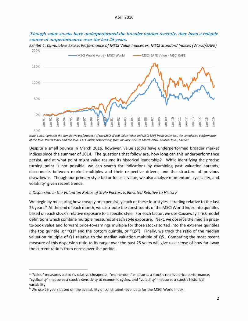
So why invest in value at all? Its track record is perhaps value’s strongest advocate. Over longer periods,

value stocks have outperformed the markets fairly consistently. As Exhibit 1 illustrates, despite short

periods of weakness, value indices have outperformed benchmark indices over the past 25 years.

Additionally, buying inexpensive or “cheap,” unloved stocks makes intuitive sense. If a stock trades lower

but fundamentals remain unchanged, the upside to downside ratio improves and the increasingly

asymmetric return profile becomes more attractive. At Causeway, we like to add to positions on these

price declines. It may be difficult to do at the time, but this discipline is why you hire an active value

manager. Although timing cannot be predicted, eventually value works, the pendulum swings the other

way, and cheap stocks ultimately outperform. Contrarian investors who can “stomach” value drawdowns

are rewarded for their patience by the subsequent snap-back and re-rating.

April 2016

2

Though value stocks have underperformed the broader market recently, they been a reliable

source of outperformance over the last 25 years.

Exhibit 1. Cumulative Excess Performance of MSCI Value Indices vs. MSCI Standard Indices (World/EAFE)

Note: Lines represent the cumulative performance of the MSCI World Value Index and MSCI EAFE Value Index less the cumulative performance

of the MSCI World Index and the MSCI EAFE Index, respectively, from January 1991 to March 2016. Source: MSCI, FactSet

Despite a small bounce in March 2016, however, value stocks have underperformed broader market

indices since the summer of 2014. The questions that follow are, how long can this underperformance

persist, and at what point might value resume its historical leadership? While identifying the precise

turning point is not possible, we can search for indications by examining past valuation spreads,

disconnects between market multiples and their respective drivers, and the structure of previous

drawdowns. Though our primary style factor focus is value, we also analyze momentum, cyclicality, and

volatilitya given recent trends.

I. Dispersion in the Valuation Ratios of Style Factors Is Elevated Relative to History

We begin by measuring how cheaply or expensively each of these four styles is trading relative to the last

25 years.b At the end of each month, we distribute the constituents of the MSCI World Index into quintiles

based on each stock’s relative exposure to a specific style. For each factor, we use Causeway’s risk model

definitions which combine multiple measures of each style exposure. Next, we observe the median price-

to-book value and forward price-to-earnings multiple for those stocks sorted into the extreme quintiles

(the top quintile, or “Q1” and the bottom quintile, or “Q5”). Finally, we track the ratio of the median

valuation multiple of Q1 relative to the median valuation multiple of Q5. Comparing the most recent

measure of this dispersion ratio to its range over the past 25 years will give us a sense of how far away

the current ratio is from norms over the period.

a “Value” measures a stock’s relative cheapness, “momentum” measures a stock’s relative price performance, “cyclicality” measures a stock’s sensitivity to economic cycles, and “volatility” measures a stock’s historical variability. b We use 25 years based on the availability of constituent-level data for the MSCI World Index.

-50%

0%

50%

100%

150%

200%

Jan

-91

Jan

-92

Jan

-93

Jan

-94

Jan

-95

Jan

-96

Jan

-97

Jan

-98

Jan

-99

Jan

-00

Jan

-01

Jan

-02

Jan

-03

Jan

-04

Jan

-05

Jan

-06

Jan

-07

Jan

-08

Jan

-09

Jan

-10

Jan

-11

Jan

-12

Jan

-13

Jan

-14

Jan

-15

Jan

-16

MSCI World Value - MSCI World MSCI EAFE Value - MSCI EAFE

April 2016

3

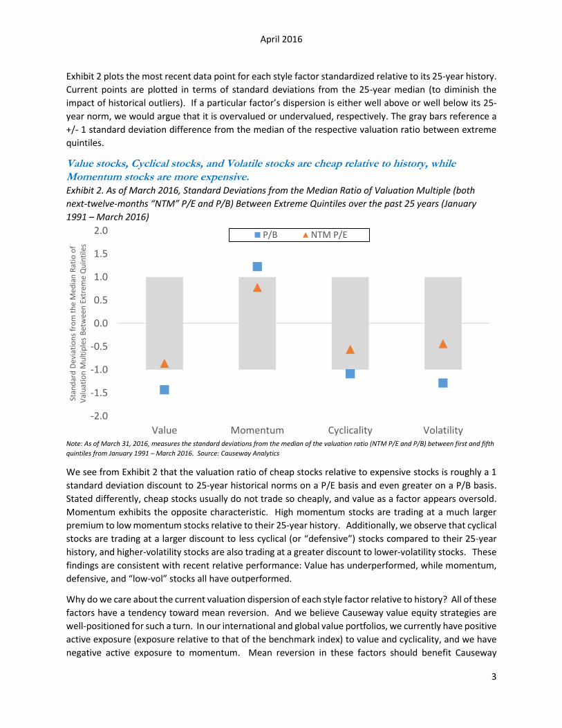
Exhibit 2 plots the most recent data point for each style factor standardized relative to its 25-year history.

Current points are plotted in terms of standard deviations from the 25-year median (to diminish the

impact of historical outliers). If a particular factor’s dispersion is either well above or well below its 25-

year norm, we would argue that it is overvalued or undervalued, respectively. The gray bars reference a

+/- 1 standard deviation difference from the median of the respective valuation ratio between extreme

quintiles.

Value stocks, Cyclical stocks, and Volatile stocks are cheap relative to history, while

Momentum stocks are more expensive.

Exhibit 2. As of March 2016, Standard Deviations from the Median Ratio of Valuation Multiple (both

next-twelve-months “NTM” P/E and P/B) Between Extreme Quintiles over the past 25 years (January

1991 – March 2016)

Note: As of March 31, 2016, measures the standard deviations from the median of the valuation ratio (NTM P/E and P/B) between first and fifth

quintiles from January 1991 – March 2016. Source: Causeway Analytics

We see from Exhibit 2 that the valuation ratio of cheap stocks relative to expensive stocks is roughly a 1

standard deviation discount to 25-year historical norms on a P/E basis and even greater on a P/B basis.

Stated differently, cheap stocks usually do not trade so cheaply, and value as a factor appears oversold.

Momentum exhibits the opposite characteristic. High momentum stocks are trading at a much larger

premium to low momentum stocks relative to their 25-year history. Additionally, we observe that cyclical

stocks are trading at a larger discount to less cyclical (or “defensive”) stocks compared to their 25-year

history, and higher-volatility stocks are also trading at a greater discount to lower-volatility stocks. These

findings are consistent with recent relative performance: Value has underperformed, while momentum,

defensive, and “low-vol” stocks all have outperformed.

Why do we care about the current valuation dispersion of each style factor relative to history? All of these

factors have a tendency toward mean reversion. And we believe Causeway value equity strategies are

well-positioned for such a turn. In our international and global value portfolios, we currently have positive

active exposure (exposure relative to that of the benchmark index) to value and cyclicality, and we have

negative active exposure to momentum. Mean reversion in these factors should benefit Causeway

-2.0

-1.5

-1.0

-0.5

0.0

0.5

1.0

1.5

2.0

Value Momentum Cyclicality Volatility

Stan

dar

d D

evia

tio

ns

fro

m t

he

Med

ian

Rat

io o

f V

alu

atio

n M

ult

iple

s B

etw

een

Ext

rem

e Q

uin

tile

s

P/B NTM P/E

April 2016

4

portfolios. It is important to emphasize that these active positions do not represent attempts to “time”

factors. Rather, as value investors, we will generally have positive active exposure to undervalued factors

and negative active exposure to overvalued factors.

II. Spreads in Fundamental Drivers Do Not Explain Spreads in Current Valuation Multiples

Another way to gauge the degree of disconnect in factor valuations is to investigate the drivers behind

the specific metrics that we have been using: price-to-earnings and price-to-book value multiples. Using

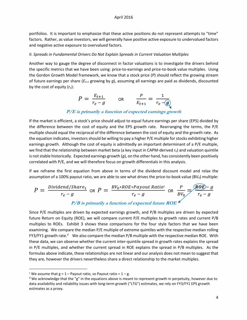
the Gordon Growth Model framework, we know that a stock price (P) should reflect the growing stream

of future earnings per share (Et+1 growing by g), assuming all earnings are paid as dividends, discounted

by the cost of equity (re):

𝑃 = 𝐸𝑡+1

𝑟𝑒 − 𝑔 OR

𝑃

𝐸𝑡+1=

1

𝑟𝑒 − 𝒈

P/E is primarily a function of expected earnings growth

If the market is efficient, a stock’s price should adjust to equal future earnings per share (EPS) divided by

the difference between the cost of equity and the EPS growth rate. Rearranging the terms, the P/E

multiple should equal the reciprocal of the difference between the cost of equity and the growth rate. As

the equation indicates, investors should be willing to pay a higher P/E multiple for stocks exhibiting higher

earnings growth. Although the cost of equity is admittedly an important determinant of a P/E multiple,

we find that the relationship between market beta (a key input in CAPM-derived re) and valuation quintile

is not stable historically. Expected earnings growth (g), on the other hand, has consistently been positively

correlated with P/E, and we will therefore focus on growth differentials in this analysis.

If we reframe the first equation from above in terms of the dividend discount model and relax the

assumption of a 100% payout ratio, we are able to see what drives the price-to-book value (BV0) multiple:

𝑃 = 𝐷𝑖𝑣𝑖𝑑𝑒𝑛𝑑/𝑆ℎ𝑎𝑟𝑒1

𝑟𝑒 − 𝑔 OR 𝑃 =

𝐵𝑉0∗𝑅𝑂𝐸∗𝑃𝑎𝑦𝑜𝑢𝑡 𝑅𝑎𝑡𝑖𝑜c

𝑟𝑒 − 𝑔 OR

𝑃

𝐵𝑉0=

𝑹𝑶𝑬 − 𝑔

𝑟𝑒 − 𝑔

P/B is primarily a function of expected future ROE

Since P/E multiples are driven by expected earnings growth, and P/B multiples are driven by expected

future Return on Equity (ROE), we will compare current P/E multiples to growth rates and current P/B

multiples to ROEs. Exhibit 3 shows these comparisons for the four style factors that we have been

examining. We compare the median P/E multiple of extreme quintiles with the respective median rolling

FY3/FY1 growth rate.d We also compare the median P/B multiple with the respective median ROE. With

these data, we can observe whether the current inter-quintile spread in growth rates explains the spread

in P/E multiples, and whether the current spread in ROE explains the spread in P/B multiples. As the

formulas above indicate, these relationships are not linear and our analysis does not mean to suggest that

they are, however the drivers nevertheless share a direct relationship to the market multiples.

c We assume that g = 1 – Payout ratio, so Payout ratio = 1 – g. d We acknowledge that the “g” in the equations above is meant to represent growth in perpetuity, however due to data availability and reliability issues with long-term growth (“LTG”) estimates, we rely on FY3/FY1 EPS growth estimates as a proxy.

April 2016

5

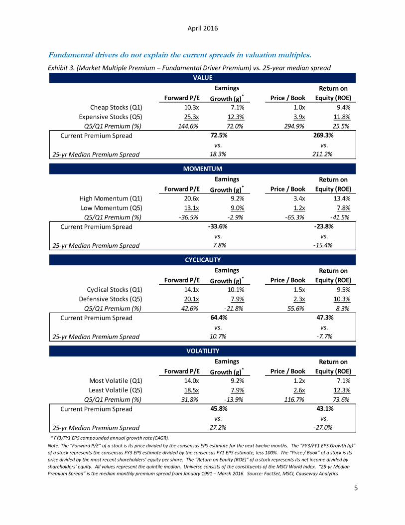
Fundamental drivers do not explain the current spreads in valuation multiples.

Exhibit 3. (Market Multiple Premium – Fundamental Driver Premium) vs. 25-year median spread

Note: The “Forward P/E” of a stock is its price divided by the consensus EPS estimate for the next twelve months. The “FY3/FY1 EPS Growth (g)”

of a stock represents the consensus FY3 EPS estimate divided by the consensus FY1 EPS estimate, less 100%. The “Price / Book” of a stock is its

price divided by the most recent shareholders’ equity per share. The “Return on Equity (ROE)” of a stock represents its net income divided by

shareholders’ equity. All values represent the quintile median. Universe consists of the constituents of the MSCI World Index. “25-yr Median

Premium Spread” is the median monthly premium spread from January 1991 – March 2016. Source: FactSet, MSCI, Causeway Analytics

VALUE

Forward P/E

Earnings

Growth (g)* Price / Book

Return on

Equity (ROE)

Cheap Stocks (Q1) 10.3x 7.1% 1.0x 9.4%

Expensive Stocks (Q5) 25.3x 12.3% 3.9x 11.8%

Q5/Q1 Premium (%) 144.6% 72.0% 294.9% 25.5%

Current Premium Spread

vs. vs.

25-yr Median Premium Spread

MOMENTUM

Forward P/E

Earnings


Return on

Equity (ROE)

High Momentum (Q1) 20.6x 9.2% 3.4x 13.4%

Low Momentum (Q5) 13.1x 9.0% 1.2x 7.8%

Q5/Q1 Premium (%) -36.5% -2.9% -65.3% -41.5%


vs. vs.


CYCLICALITY

Forward P/E

Earnings


Return on

Equity (ROE)

Cyclical Stocks (Q1) 14.1x 10.1% 1.5x 9.5%

Defensive Stocks (Q5) 20.1x 7.9% 2.3x 10.3%

Q5/Q1 Premium (%) 42.6% -21.8% 55.6% 8.3%


vs. vs.


VOLATILITY

Forward P/E

Earnings


Return on

Equity (ROE)

Most Volatile (Q1) 14.0x 9.2% 1.2x 7.1%

Least Volatile (Q5) 18.5x 7.9% 2.6x 12.3%

Q5/Q1 Premium (%) 31.8% -13.9% 116.7% 73.6%


vs. vs.


* FY3/FY1 EPS compounded annual growth rate (CAGR).

72.5% 269.3%

18.3% 211.2%

-33.6% -23.8%

45.8% 43.1%

27.2% -27.0%

7.8% -15.4%

64.4% 47.3%

10.7% -7.7%

April 2016

6

In the cases of value, cyclicality, and volatility, the spread in market multiples far outpaces the spread in

the underlying driver. This shows yet again that value stocks, cyclical stocks, and higher-volatility stocks

are trading at much bigger discounts to their opposing peers relative to the underlying driver. Admittedly,

a valuation premium is probably warranted from more “stable” defensive and low-volatility stocks, but

the current valuation spreads are also much greater than their 25-year median spreads (see the boxed

comparison). In the case of momentum, high-momentum stocks trade at a larger premium than the

underlying drivers or historical spreads would justify. This is consistent with our conclusions in Exhibit 2.

III. Value Has Recovered Quickly in Past Drawdowns While Momentum Has Drawn Down Quickly

Finally, in the case of value and momentum specifically, it is helpful to examine the characteristics of past

drawdowns for insights into mean reversion trends. Using our proprietary risk model, which strips out

the effects of individual styles from country, sector, currency, and idiosyncratic effects, we seek to isolate

and link the historical returns attributable to value. These would be the theoretical returns that any

portfolio with a pure exposure to value (holding all other factors constant) would have recognized. And

as such, we believe they offer a good proxy for the effects impacting value portfolios such as Causeway’s

international and global value strategies. Exhibit 4 analyzes the characteristics of previous value

drawdowns over the past 25 years (1991 - March 2016) using a broad universe of global equities in the

developed markets.

Value drawdowns tend to snap back quickly.

Exhibit 4. Drawdowns of Causeway Risk Model’s Value factor controlling for style, sector, country, and currency returns (January 1991 – March 2016)

Note: Drawdown is the peak-to-trough decline during a specific period, measured as the percentage change between the peak and the trough.

The universe represented in the chart above consists of developed markets global equities, including securities from certain emerging markets in

the investable universe of Causeway’s fundamental value strategies, subject to minimum liquidity thresholds, that are used in Causeway’s

proprietary quantitative risk model. Cumulative return is calculated by compounding periodic returns to this risk factor. Source: Causeway Analytics

For this analysis, we define a drawdown as any decline lasting two or more months in order to avoid single

down months. The average number of months to trough was 6.6 months, and average recovery period

-10%

-9%

-8%

-7%

-6%

-5%

-4%

-3%

-2%

-1%

0%

Jan

-91

Jan

-92

Jan

-93

Jan

-94

Jan

-95

Jan

-96

Jan

-97

Jan

-98

Jan

-99

Jan

-00

Jan

-01

Jan

-02

Jan

-03

Jan

-04

Jan

-05

Jan

-06

Jan

-07

Jan

-08

Jan

-09

Jan

-10

Jan

-11

Jan

-12

Jan

-13

Jan

-14

Jan

-15

Jan

-16

Cu

mu

lati

ve D

raw

do

wn

Months % of Total Months

Drawing Down 119 39%

Recovering 82 27%

Not In Drawdown 102 34%

All Months in Chart 303 100%

April 2016

7

was 4.6 months, equating to an average total drawdown period of approximately 11 months. Two

observations can be drawn from these statistics. First, we are currently 15 months into a drawdown for

value (12 months if the December trough holds), well above the typical trough period of 6.6

months. Second, the average recovery period from a trough is much shorter than the period to the

trough. Returns to value recover quickly, which means that attempting to time the bottom may result in

a missed recovery. In fact, looking at the table in Exhibit 4, we see that over the past 25+ years, 39% of

months were spent drawing down, while only 27% were recovering. This is also consistent with the

positive skew in returns to value, indicating that the magnitude of positive returns eclipses the more

numerous, smaller declines. Out of the four factors we have discussed, value is the only one with a positive

skew (meaning that the other factors experience larger-magnitude negative returns).

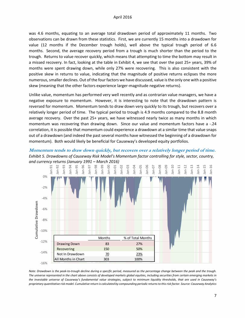
Unlike value, momentum has performed very well recently and as contrarian value managers, we have a

negative exposure to momentum. However, it is interesting to note that the drawdown pattern is

reversed for momentum. Momentum tends to draw down very quickly to its trough, but recovers over a

relatively longer period of time. The typical period to trough is 4.9 months compared to the 8.8 month

average recovery. Over the past 25+ years, we have witnessed nearly twice as many months in which

momentum was recovering than drawing down. Since our value and momentum factors have a -.24

correlation, it is possible that momentum could experience a drawdown at a similar time that value snaps

out of a drawdown (and indeed the past several months have witnessed the beginning of a drawdown for

momentum). Both would likely be beneficial for Causeway’s developed equity portfolios.

Momentum tends to draw down quickly, but recovers over a relatively longer period of time.

Exhibit 5. Drawdowns of Causeway Risk Model’s Momentum factor controlling for style, sector, country, and currency returns (January 1991 – March 2016)

Note: Drawdown is the peak-to-trough decline during a specific period, measured as the percentage change between the peak and the trough.

The universe represented in the chart above consists of developed markets global equities, including securities from certain emerging markets in

the investable universe of Causeway’s fundamental value strategies, subject to minimum liquidity thresholds, that are used in Causeway’s

proprietary quantitative risk model. Cumulative return is calculated by compounding periodic returns to this risk factor. Source: Causeway Analytics

-16%

-14%

-12%

-10%

-8%

-6%

-4%

-2%

0%

Jan

-91

Jan

-92

Jan

-93

Jan

-94

Jan

-95

Jan

-96

Jan

-97

Jan

-98

Jan

-99

Jan

-00

Jan

-01

Jan

-02

Jan

-03

Jan

-04

Jan

-05

Jan

-06

Jan

-07

Jan

-08

Jan

-09

Jan

-10

Jan

-11

Jan

-12

Jan

-13

Jan

-14

Jan

-15

Jan

-16

Cu

mu

lati

ve D

raw

do

wn

Months % of Total Months

Drawing Down 83 27%

Recovering 150 50%

Not In Drawdown 70 23%

All Months in Chart 303 100%

April 2016

8

Summary

The recent underperformance of value as an investment style has created a strong headwind for value

managers, prompting the question, when will value resume its historical outperformance? We seek to

answer this question by measuring the magnitude of the current dislocation from three perspectives. We

find that value stocks are trading at a much larger discount to their more expensive peers relative to

history. They are also much more disconnected from their underlying valuation drivers relative to history.

And finally, the drawdown in value has already outpaced the average previous decline. Although recovery

could still take longer given the depth of the current drawdown, each of these analyses argue in favor of

mean reversion for value. We believe the time to emphasize value has arrived.

This paper expresses the portfolio managers’ views as of April 2016 and should not be relied on as research or investment advice regarding any stock. These views and any portfolio holdings and characteristics are subject to change. There is no guarantee that any forecasts made will come to pass.

International investing may involve risk of capital loss from unfavorable fluctuations in currency values, from differences in generally accepted accounting principles, or from economic or political instability in other nations.

The MSCI EAFE Index is a free float adjusted market capitalization weighted index, designed to measure developed market equity performance excluding the U.S. and Canada, consisting of 21 stock markets in Europe, Australasia, and the Far East. The MSCI World Index is a free float-adjusted market capitalization index, designed to measure developed market equity performance, consisting of 23 developed country indices, including the U.S. The MSCI EAFE Value and MSCI World Value Indices are subsets of these indices, and target 50% coverage of the MSCI EAFE Index and MSCI World Index, respectively, with value investment style characteristics for index construction using three variables: book value to price, 12-month forward earnings to price, and dividend yield. The indices are gross of withholding taxes, assume reinvestment of dividends and capital gains, and assume no management, custody, transaction or other expenses. It is not possible to invest directly in an Index.

MSCI has not approved, reviewed or produced this report, makes no express or implied warranties or representations and is not liable whatsoever for any data in the report. You may not redistribute the MSCI data or use it as a basis for other indices or investment products.

“Beta” is a measure of the risk potential of a stock or an investment portfolio expressed as a ratio of the stock's or portfolio's volatility to the volatility of the market as a whole.

“CAPM” or the “Capital Asset Pricing Model” provides a formula that calculates the expected return on a security based on its level of risk. The formula for the capital asset pricing model is the risk free rate plus beta times the difference of the return on the market and the risk free rate.

“Gordon Growth Model” is used to determine the intrinsic value of a stock based on a future series of dividends that grow at a constant rate. Given a dividend per share that is payable in one year, and the assumption the dividend grows at a constant rate in perpetuity, the model solves for the present value of the infinite series of future dividends.

“Standard Deviation” is a measure that is used to quantify the amount of variation or dispersion of a set of data values. The more spread apart the data, the higher the deviation. Standard deviation is calculated as the square root of variance.

DRAFT AGENDA AS OF 09/09/09 - Tucson · Formal Evaluation of Active Managers ... March 2016 Summary Performance Report ... Alliance S&P Index 83,139,473 11.71% 475 5,247,538 77,891,461

Documents