DRAFT 1.2 Base Numeric Nutrient Standards Implementation Guidance* *Retitled from earlier drafts to reflect the more encompassing nature of this document. Previous draft number was 7.3 December 2013 Prepared by: Water Quality Planning Bureau, Water Quality Standards Section Montana Department of Environmental Quality 1520 E. Sixth Avenue P.O. Box 200901 Helena, MT 59620-0901 WQPBWQSTR-002

Welcome message from author
This document is posted to help you gain knowledge. Please leave a comment to let me know what you think about it! Share it to your friends and learn new things together.
Transcript
DRAFT 1.2 Base Numeric Nutrient Standards Implementation Guidance* *Retitled from earlier drafts to reflect the more encompassing nature of this document. Previous draft number was 7.3
December 2013 Prepared by: Water Quality Planning Bureau, Water Quality Standards Section Montana Department of Environmental Quality 1520 E. Sixth Avenue P.O. Box 200901 Helena, MT 59620-0901
WQPBWQSTR-002

Suggested citation: Montana Department of Environmental Quality, 2013. Base Numeric Nutrient Standards Implementation Guidance. DRAFT, version 1.1. Helena, MT: Montana Dept. of Environmental Quality
Nutrient Standards Implementation Guidance – Table of Contents
TABLE OF CONTENTS
...................................................................................................................................................................... 1
Table of Contents ........................................................................................................................................... i
List of Figures ................................................................................................................................................ ii
Acronyms ..................................................................................................................................................... iv
1.0 Introduction ............................................................................................................................................ 6
1.1 Definitions ........................................................................................................................................... 6
2.0 Defined Nutrient-reduction Steps for Permittees Operating under a General Nutrient Standards Variance ........................................................................................................................................................ 6
3.0 The Evaluation Process for Individual Variances: Public-sector Permittees ........................................... 7
3.1 Substantial and Widespread Economic Impacts: Process Overview .................................................. 8
3.2 Completing the Substantial and Widespread Assessment Spreadsheet .......................................... 10
3.3 Determining the Target Cost of the Pollution Control Project ......................................................... 11
4.0 The Evaluation Process for Individual Variances: Private-sector Permittees ....................................... 13
4.1 Substantial and Widespread Economic Impacts: Process Overview ................................................ 13
4.2 Completing the Substantial and Widespread Assessment Spreadsheet .......................................... 14
4.3 Cost-cap (or other solution) for Private Entities ............................................................................... 15
5.0 Streamlined Methods for Developing Site-specific Numeric Nutrient Criteria .................................... 15
5.1 Background and Rationale ................................................................................................................ 15
5.2 Site-specific Methods ........................................................................................................................ 16
5.2.1 Principal Site-specific Methods .................................................................................................. 16
5.2.2 Other Methods ........................................................................................................................... 18
5.3 Confirmation of Biological Health, and Minimum Dataset ............................................................... 19
5.3.1 Assessment of the Biological Health of the Stream ................................................................... 19
5.3.2 Dataset Minimum ...................................................................................................................... 20
5.3.3 Consideration of the Other Nutrient ......................................................................................... 20
5.4 Case-study Example .......................................................................................................................... 21
5.4.1 Data Summary for Stream X (in Middle Rockies Ecoregion) ...................................................... 21
5.4.2 The Assessment of Stream X ...................................................................................................... 21
5.4.3 Site-specific Criteria Derivation for Stream X using the Streamlined Approach........................ 21
5.5 References ........................................................................................... Error! Bookmark not defined.
6.0 Guidelines for Developing Site-specific Numeric Nutrient Criteria via Water Quality Modeling, and the Relation of these Criteria to Individual Nutrient Standards Variances ................................................ 22
6.1 Mechanistic and Empirical Modeling Approaches for Establishing Individual Variances and (Potentially) Reach-specific Nutrient Standards ..................................................................................... 23
5/15/12 Draft i

Nutrient Standards Implementation Guidance – Table of Contents
6.2 Protection of Downstream Beneficial Uses ...................................................................................... 24
6.3. Unwarranted Cost and Economic Impact ........................................................................................ 24
6.4 Department Adoption and Periodic Review of the Individual Variance ........................................... 25
7.0 References ............................................................................................................................................ 25
Appendix A: Recommendations for Sampling and Modeling the East Gallatin River to Accomplish Multiple Objectives ..................................................................................................................................... 27
LIST OF FIGURES
Figure 2-1. Sliding scale for determining cost cap based on a community’s secondary score. .................. 12
5/15/12 Draft ii

Nutrient Standards Implementation Guidance – Table of Contents
5/15/12 Draft iii
Nutrient Standards Implementation Guidance– Acronyms
ACRONYMS
Acronym Definition DEQ Department of Environmental Quality (Montana) EPA Environmental Protection Agency (US) LMI Low to Moderate Income MCA Montana Code Annotated MHI Median Household Income
5/15/12 Draft iv

Nutrient Standards Implementation Guidance– Acronyms
5/15/12 Draft v

6
1.0 INTRODUCTION
This document provides guidance pertaining to implementation of Montana’s base numeric nutrient standards and variances from those standards. The remaining sections address the following topics: Section 2.0: For permittees operating under a general nutrient standards variance, this section provides the defined effluent limits (i.e., nutrient reduction steps) to be met over several permit cycles of the general variance Section 3.0: Provides guidance for the development of Individual Nutrient Standards Variances for public-sector entities, based on economic factors; Section 4.0: Provides guidance for the development of Individual Nutrient Standards Variances for private-sector entities, based on economic factors; Section 5.0: Outlines a streamlined approach for developing site-specific numeric nutrient criteria for streams or rivers where full biological support is demonstrated but where the existing nutrient concentrations exceed applicable nutrient standards; and Section 6.0: Provides a detailed, data-intensive modeling approach for developing site-specific numeric nutrient criteria. This approach lends itself to the development of individual variances for dischargers.
1.1 DEFINITIONS 1. Limits of technology means wastewater treatment processes for the removal of nitrogen and
phosphorus compounds from wastewater that can consistently achieve a concentration of 70 µg TP/L and 4,000 µg TN/L.
1.2. Pollution control project means an upgrade to a wastewater treatment facility and all directly relevant infrastructure.
2.0 DEFINED NUTRIENT-REDUCTION STEPS FOR PERMITTEES OPERATING UNDER A GENERAL NUTRIENT STANDARDS VARIANCE
The Department and the Nutrient Work Group developed a series of defined nutrient-reduction steps to be taken over time and that are specific to recipients of general nutrient standards variances. Per §75-5-313 [8], MCA, general nutrient standards variance may be established for no more than 20 years. The intent of establishing nutrient reduction steps upfront for most of the 20 year period is to provide permittees regulatory certainty well out into the future. This in turn allows for better facility planning and financing. State law still requires the Department to review triennially the general variance concentrations (§75-5-313 [7][b], MCA). However, the Department will only supersede the reduction steps defined here if substantial cost reductions for existing technology have occurred, or technological innovations have allowed for nutrient reductions well beyond the defined steps and those technologies can be readily implemented on facilities in Montana.

7
For the purposes of permit development, the values provided below apply to recipients of general nutrient standards variances and the concentrations should be viewed as long-term averages.
1. For facilities > 1 million gallons per day: A. By 2016 (or first receipt of general nutrient standards variance): 10 mg TN/L, 1.0 mg TP/L B. Next permit cycle (5 year later): 8 mg TN/L, 0.8 mg TP/L C. Next permit cycle (5 years later): 8 mg TN/L, 0.3 5 mg TP/L D. Next permit cycle (5 years later): 5 mg TN/L, 0.15 mg TP/L 2. For facilities < 1 million gallons per day: A. By 2016 (or first receipt of general nutrient standards variance): 15 mg TN/L, 2.0 mg TP/L B. Next permit cycle (5 year later): 12 mg TN/L, 2.0 mg TP/L C. Next permit cycle (5 years later): 10 mg TN/L, 1.0 mg TP/L D. Next permit cycle (5 years later): 8 mg TN/L, 0.8 mg TP/L 3. For lagoons not designed to actively remove nutrients: A. By 2016 (or first receipt of general nutrient standards variance): Maintain current lagoon performance and commence nutrient monitoring in the effluent B. Next permit cycles (5 years later): Implement BMPs identified during optimization study
3.0 THE EVALUATION PROCESS FOR INDIVIDUAL VARIANCES: PUBLIC-SECTOR PERMITTEES
Montana law allows for the granting of nutrient standards variances based on the specific economic and financial conditions of a permittee (§75-5-313 [1], MCA). These variances, referred to as individual nutrient standards variances (“individual variances”), may be granted on a case-by-case basis because the attainment of the base numeric nutrient standards is precluded due to economic impacts, limits of technology, or both. Individual variances may only be granted to a permittee after the permittee has made a demonstration to the Department that adverse, significant economic impacts would occur, the limits of technology have been reached, or both, and that there are no reasonable alternatives to discharging into state waters. The processes by which the demonstration is made are provided here, and were developed in conjunction with Montana Nutrient Work Group. Methods outlined below are Montana’s modifications to methods presented in U.S. Environmental Protection Agency (1995). If adverse substantial and widespread economic impacts to a community trying to comply with base numeric nutrient standards are demonstrated, the facility upgrade cost-cap will be determined via a sliding scale as proposed by EPA in its September 10, 2010 memo “EPA Guidance on Variances”, reference No. 8EPR-EP. In taking this approach, the Department has assumed that most permittees who cannot comply with the base numeric nutrient standards (DEQ-12, Part A) would pursue a general variance (DEQ-12, Part B). Therefore, individual variances discussed here are generally for permittees for whom significant

8
economic impacts would occur even at the general variance treatment levels. For communities with secondary scores (discussed further below) of 1.5 or lower, the cost cap for the upgrade would be set at 1.0% or lower of the median household income (MHI) for a town, including existing wastewater fees. If the cost cap were below existing wastewater rates, then no further action would be required. The Nutrient Work Group has indicated that 1.0% of MHI is an acceptable cost cap for a community to expend on wastewater treatment where economic hardship due to meeting base numeric nutrient standards has been demonstrated. Higher Secondary scores would lead to a higher MHI cost cap. A small flow chart of the overall process is as follows:
NO
YES
3.1 SUBSTANTIAL AND WIDESPREAD ECONOMIC IMPACTS: PROCESS OVERVIEW The following is an overview of the steps required to carry out a substantial and widespread economic analysis for a public-sector permittee. The evaluation can be undertaken directly in an Excel spreadsheet template which contains instructions. The template is called “PublicEntity_Worksheet_EPACostModel_2013.xlsx” and is available from the Department. Step 1: Verify project costs that would occur from meeting the base numeric nutrient criteria and calculate the annual cost of the new pollution control project. Step 2: Calculate total annualized pollution control cost per household including existing wastewater fees and the new pollution control project (manifested as an increase in the household wastewater bill). Steps 3-5: The Substantial Test Step 3: Calculate and evaluate the Municipal Preliminary Screener score based on the new wastewater fees and the town’s Median Household Income. This step identifies communities that can readily pay for the pollution control project vs. those that cannot. Note: If the public entity passes a significant portion of the pollution control costs along to private facilities or firms, then the review procedures outlined in Chapter 3 of EPA (1995) for 'Private Entities' should also be consulted to determine the impact on the private entities. Step 4: Calculate the Secondary Test to get a secondary score. This measurement incorporates a characterization of the socio-economic and financial well-being of households in the community where the wastewater plant is located. It comprises five evaluation parameters which are then compared
Can the permittee affordably meet the General Variance?
Permittee meets the General Variance with upgrades
Permittee applies for an individual variance.
Permittee demonstrates they cannot meet base standards using significant and widespread test.
After looking at all alternatives to meeting the base criteria, permittee takes Secondary Score and uses sliding scale to determine cost cap. Permittee works with DEQ to find a variance solution based on the cap
9
against state averages for a score. The scores of the five parameters are averaged to provide the secondary test score for a given community. A secondary score can range from 1.0 to 3.0. 3.0 is a strong score and 1.0 is a weak score. Note: The Secondary Score is based on the assumption that the ability of a community to finance a project may be dependent upon existing household financial conditions within that community. Step 5: Assess where the community falls in the substantial impacts matrix. This matrix evaluates whether or not a given community is expected to incur substantial economic impacts due to the implementation of the pollution control costs. If the applicant can demonstrate substantial impacts, then the applicant moves on to the widespread test. If the applicant cannot demonstrate substantial impacts, then they will not perform the widespread test; they will be required to meet the base numeric nutrient standards, or may request a general variance if they can discharge at the general variance concentrations defined in Department Circular DEQ-12, Part B. Note: The evaluation of substantial impacts resulting from compliance with base numeric nutrient standards includes two elements; (1) financial impacts to the public entity as measured in Step 3 (reflected in increased household wastewater fees), and (2) current socio-economic conditions of the community as measured in Step 4. Governments have the authority to levy taxes and distribute pollution control costs among households and businesses according to the tax base. Similarly, sewage authorities charge for services, and thus can recover pollution control costs through user’s fees. In both cases, a substantial impact will usually affect the wider community. Whether or not the community faces substantial impacts depends on both the cost of the pollution control and the general financial and economic health of the community. Step 6: The Widespread Test Step 6: If impacts of meeting base numeric nutrient criteria are expected to be substantial, then the applicant goes on to demonstrate whether or not the impacts are expected to be widespread. The Widespread test consists of questions that ask the permittee about current economic, social and population trends in the affected area (usually the committee and possibly outlying areas tied to the community). The permittee is then asked to estimate the effects of higher wastewater costs on each of these trends. Further optional questions are asked about the effects of higher wastewater costs on things like city debt limits, improved water quality, future development patterns, and other factors that the applicant may want to add. Note: Estimated changes in socio-economic indicators of the community and other geographical areas tied to the community as a result of pollution control costs and will be used to determine whether widespread impacts would occur. Step 7: Final Determination of Substantial and Widespread Economic Impacts Step 7: If widespread impacts are also demonstrated, then a permittee is eligible for an individual variance after having demonstrated to the Department that they considered alternatives to discharging (including but not limited to trading, land application, and permit compliance schedules). If widespread impacts have not been demonstrated, then the permittee is not eligible for an individual variance (however, the permittee may still receive a general variance if they can comply with the end-of-pipe treatment requirements thereof).
10
3.2 COMPLETING THE SUBSTANTIAL AND WIDESPREAD ASSESSMENT SPREADSHEET Detailed steps for completing the substantial and widespread cost assessment are found in the spreadsheet template “PublicEntity_Worksheet_EPACostModel_2013.xlsx” available from the Department and on the Nutrient Workgroup website. Readers should refer to that spreadsheet, as it is self-explanatory and instructions are found throughout. Below are a few additional details which may help clarify some of the steps:
1. Start at the far left tab of the spreadsheet (“Instructions [Steps to be Taken]”) and review the instructions. They are the same steps outlined in Section 2.1 above, but in more detail. Proceed to subsequent tabs to the right, making sure not to skip any of worksheets A through F.
2. Summarize the project on Worksheet A. 3. Detail the costs of the project on Worksheet B. 4. Calculated the annual cost per household of existing and expected new water treatment costs
on Worksheet C. 5. On Worksheet D, carefully read the text in blue and compare it to the results from the MHI test
and the community’s Low to Moderate Income (LMI) level. Based on this screener, the evaluation will either terminate (i.e., it has been shown that the water pollution control is clearly affordable), or will continue to the secondary tests on the next tab which is Worksheet E1.
6. On Worksheet E, note the linkages to websites and phone numbers where the information requested can be obtained. Then use this information to fill in Worksheet F where a secondary score is calculated.
7. The next tab, ‘Substantial Impacts Matrix’, shows if the community has demonstrated substantial impacts (or not). Those that have clearly demonstrated substantial impacts as well as those that are ‘borderline’ move on to the widespread tests.
8. On the ‘DEQ Widespread Criteria’ tab, complete the four descriptive questions. Then, complete the six primary questions and determine the outcome as to whether impacts are widespread. If still unclear, complete the additional secondary questions and again evaluate.
9. In order to be eligible for an individual variance, both substantial and widespread tests must be satisfied.
10. If substantial and widespread impacts are demonstrated, then the permittee moves on to the next tab, Worksheet I, Remedy. In this step, the permittee examines and reports whether there are “reasonable alternatives” to the individual variance that “preclude” the need for an individual variance. If not, then then the cost the permittee will need to expend towards the pollution control project will be based on the sliding scale (see below). The cost cap is determined as a percentage of the community’s MHI, and the key driver of the required cost cap is the Secondary Score.
The difference between the cost cap MHI from the sliding scale and what is currently being paid (also in MHI) is the additional money that can go towards the pollution control project. Once the amount of money available is determined, DEQ and the applicant will look at both capital and O&M investments
1 The Department appended the LMI test to EPA’s Municipal Preliminary Screener at this step in the process. This was done in order to address communities in which the income distribution is skewed such that there is a large proportion of high- and low-income individuals, but less in the middle near the median household income. As modified, the test should assure that such communities will move on to the more detailed secondary tests.

11
that could be used to meet an individual variance, given what money is available. Refer to Section 3.3 below for more details on the remedy process.
3.3 THE REMEDY: DETERMINING THE TARGET COST OF THE POLLUTION CONTROL PROJECT If a permittee has demonstrated that substantial and widespread economic impacts would occur if they were to comply with the base numeric nutrient standards, and there are no reasonable alternatives to discharging (including trading, permit compliance schedules, general variances, alternative variances, or alternative effluent management loading reduction methods such as reuse, recharge, or land application), then the cost the permittee will need to expend towards the pollution control project will be based on a sliding scale (Figure 3-1). The cost cap is determined as a percentage of the community’s MHI, and the key driver of the cost cap is the secondary test (secondary score) calculated in step 4 of Section 3.1. For example, a community has demonstrated that substantial and widespread economic impacts would occur from trying to comply with the base numeric nutrient standards, and there were no reasonable alternatives to discharging. If the permittee’s average secondary score from the secondary tests was 1.5, then the annual cost cap for the pollution control project (including current wastewater fees) would be the dollar value equal to 1.0% of the community’s MHI at the time that the analysis was undertaken (see blue line, Figure 3-1). This 1.0% would include existing wastewater costs plus the new, hypothetical upgrades. If this community was already paying ≥ 1.0% of community MHI for its wastewater bill, then no additional monies would be spent on capital or O&M costs (and no additional upgrades would occur). Still, additional improvements may still be expected. The facility’s current discharge nutrient concentrations might become the basis of the community’s individual variance but the community must first look at optimization options such as operator training and use all tools available within their cost cap to improve water quality. Once those are considered, the individual variance can be developed. The difference between the cost cap MHI from the sliding scale and what is currently being paid in MHI is the additional money that can go towards the pollution control project. This amount could be zero in some cases, as in the example just given. This additional money is calculated for the whole town over 20 years (assumed life of the pollution control project) in order to see what the total amount of money available would be. The cost cap, which is given as a percentage of a community’s MHI and determined by the ‘sliding scale’ in Figure 3-1, would translate to the final wastewater bill that the community would pay after the upgrade. For example, a community with 10,000 households has a MHI of $40,000/year. The community’s secondary score is 1.5 and therefore the sliding scale indicates that 1.0% MHI needs to be expended on the pollution control project. To receive the individual variance, the per-household wastewater bill for the community would need to become, on average, $400 per year ($33.33 per month), because $400 is 1.0% of MHI in that community. If the average household in this community currently has a wastewater bill that is $300 per year ($25.00 per month), then a bill increase of $100 per year per household on average would be warranted to reach $400 per year or 1% MHI. Multiplying $100/year in an increased wastewater bill by the number of households on the system (10,000) provides the total annual dollar value available to be expended towards construction, operations, and maintenance of the wastewater

12
upgrade. In this hypothetical case, that amounts to $1 million (10,000 X $100) that could be spent per year on an upgrade project. The upgrade itself may be significantly more than $1 million in initial capital costs, but the annualized payback of capital costs plus O&M costs of the upgrade could not be more than $1 million per year. Annualizing $1 million per year over several years could allow for a substantial upgrade of several million dollars. Again, if the current wastewater bill of this town was already $400 or higher, then no additional significant capital or O&M cost upgrade would be expected (i.e., no further significant system upgrade would be required).
1
1.5
2
2.5
3
0.5 1 1.5 2 2.5
Seco
ndar
y Sc
ore
Cost Cap (Percent MHI)
Cost Cap versus Secondary Score
Cost Cap
Figure 3-1. Sliding scale for determining cost cap based on a community’s secondary score. The horizontal axis represents percentages of a community’s median household income (MHI) that the community would be expected to expend towards the pollution control project as a function of the secondary score shown on the vertical axis. DEQ looks at the town's current treatment level (TN and TP) and current treatment technology, which informs (along with the additional money amount) what the next level of treatment should be. Once the amount of money available is determined, DEQ and the applicant look at both capital and O&M investments that could be used to meet an individual variance, given what money is available. Staff from DEQ will review the application and the remedy. The staff will generally include the Department’s economist, an engineer from the Technical and Financial Assistance Bureau, staff from the Water Quality Standards Section, and staff from the Water Protection Bureau (i.e., permitting). The WWTP applicant must propose a level of water treatment greater than what they are currently meeting. If a town is already at the cost cap, then they still must look at optimization options such as operator training and use all tools available within their cost cap which could lead to water quality improvement. The variance must be established as close to the underlying numeric criteria (or general variance) as possible to show both that the highest attainable use is being realized and that further incremental progress towards the underlying standard is occurring. DEQ and the applicant will evaluate options and select the alternative that would result in the highest effluent condition that does not trigger substantial and widespread economic impacts. The decision process should include engineering costs, design, treatment effectiveness, etc. The decision regarding the pollution control project may also
13
account for facility upgrades that do not directly improve water quality. For example, if $4 million is available over 20 years for a given community, but $2 million is needed for replacing delivery system piping over that 20 years, it may be the case that only $2 million are available to directly reduce nutrient concentrations in the effluent. Finally, the final cost of the engineering project may not exactly match the dollar value associated with the percent MHI determined via Figure 3-1 (i.e., the actual project cost could be somewhat lower or somewhat higher than the dollar value equivalent for the percent MHI of the community in question). Engineers should view the dollar value equivalent of the MHI derived from Figure 3-1 as a target, to help select the most appropriate water pollution control solution for the community. In order to accommodate actual engineering costs for the project, the Department will provide flexibility around the dollar value arrived at via Figure 3-1, subject to final Department approval. When the level of treatment required has been established and accepted by the Department, it will be adopted by the Department following the Department’s formal rule making process and documented in Circular DEQ-12, Part B.
4.0 THE EVALUATION PROCESS FOR INDIVIDUAL VARIANCES: PRIVATE-SECTOR PERMITTEES
Methods outlined below are almost identical to those presented in U.S. Environmental Protection Agency (1995). If adverse substantial and widespread economic impacts to a private entity trying to comply with nutrient standards are demonstrated, the facility upgrade will be determined via approaches discussed in Section 3.3.
4.1 SUBSTANTIAL AND WIDESPREAD ECONOMIC IMPACTS: PROCESS OVERVIEW The following is an overview of the steps required to carry out a substantial and widespread economic analysis for a private-sector permittee. The evaluation can be undertaken directly in an Excel spreadsheet template which contains instructions (see Section 3.2). The template is called “PrivateEntity_Worksheet_EPACostModel_2012.xlsx” and is available from the Department. Step 1: Verify Project Costs and Calculate the Annual Cost of the Pollution control project to the private entity. Step 2: Substantial Test. Run a financial impact analysis on the private entity to assess the extent to which existing or planned activities and/or employment will be reduced as a result of meeting the water quality standards. The primary measure of whether substantial impact will occur to the private entity is profitability. The secondary measures include indicators of liquidity, solvency, and leverage. Step 3: Widespread Test. If impacts on the private entity are expected to be substantial, then the applicant goes on to demonstrate whether they are also expected to be widespread to the defined study area. Note: Estimated changes in socio-economic indicators in a defined area as a result of the additional pollution costs will be used to determine whether widespread impacts would occur.
14
Step 4: Final Determination of Substantial and Widespread Economic Impacts. If both substantial and widespread impacts are demonstrated, then a permittee is eligible for an individual variance after having demonstrated to the Department that they considered alternatives to discharging (including but not limited to trading, land application, and permit compliance schedules). If widespread impacts have not been demonstrated, then the permittee is not eligible for an individual variance (however, the permittee may still receive a general variance if they can comply with the end-of-pipe treatment requirements thereof).
4.2 COMPLETING THE SUBSTANTIAL AND WIDESPREAD ASSESSMENT SPREADSHEET Detailed steps for completing the substantial and widespread cost assessment are found in the spreadsheet template “PrivateEntity_Worksheet_EPACostModel_2012.xlsx” (available from the Department). Readers should refer to that spreadsheet, as it is self explanatory and instructions are found throughout. Detailed steps for private sector entities are also found in Chapter 3 of U.S. Environmental Protection Agency (1995). Below are a few additional details which may help clarify some of the steps:
1. Start at the far left tab of the spreadsheet (“Instructions [Steps to Take]”) and review the
instructions. They are the same steps outlined in Section 3.1 above. Proceed to subsequent tabs to the right, making sure not to skip any of the worksheets.
2. Summarize the project on Worksheet A. 3. There are no worksheets B through F on the private test. 4. The next worksheet is G where one details the costs of the project. 5. In the next tab, carefully read the ‘Substantial Impact Instructions’. 6. In worksheets H through L, the four main substantial tests are presented. For these tests, profit
and solvency ratios are calculated with and without the additional compliance costs (taking into consideration the entity's ability to increase its prices to cover part or all of the costs). Comparing these ratios to each other and to industry benchmarks provides a measure of the impact on the entity of additional wastewater costs. For profit and solvency, the main question is how these will be affected by additional pollution control costs. The Liquidity and leverage measures look at how a firm is doing right now financially, and how much additional financial burden they could take on.
7. In the Tab entitled “Substan.Impacts_Determined”, instruction is given as to how to interpret the results from the ‘Substantial’ tests in worksheets H through L.
8. If a ‘Substantial ‘ finding is made, then proceed on to the next tab. If it is not made, then a variance will not be given.
9. On the ‘DEQ Widespread Criteria’ tab, complete the descriptive questions. Then, complete the primary questions and determine the outcome as to whether impacts are widespread. If still unclear, complete the secondary questions and again evaluate.
10. In order to be eligible for an individual variance, both substantial and widespread tests must be satisfied.
11. If both substantial and widespread impacts are demonstrated from additional pollution control costs, see Section 3.3 below.

15
4.3 COST-CAP (OR OTHER SOLUTION) FOR PRIVATE ENTITIES U.S. Environmental Protection Agency (1995) provides very little guidance as to what financial expenditure should be made towards water pollution control when a private firm has demonstrated substantial and widespread impacts would occur if they complied with the standards. U.S. Environmental Protection Agency (1995) only states that “…if substantial and widespread economic and social impacts have been demonstrated, then the discharger will not have to meet the water quality standards. The discharger will, however, be expected to undertake some additional pollution control.” In cases where substantial and widespread economic impact has been demonstrated per methods outlined here in Section 3.0, the Department expects that in most cases the discharger (and their engineers) will propose to the Department some level of effluent improvement beyond that which they are currently doing, but less stringent that the general variances concentrations (which are now in statute at §75-5-313, MCA, and which will later be adopted as Department rules in 2016). A likely scenario would be that the discharger could implement a treatment technology one level less sophisticated than that required to meet the general variance concentrations. Basic definitions for different treatment levels are found in Falk et al. (2011); through 2016 the general variance requirement for dischargers > 1 MGD corresponds to level 2. When the discharger and the Department have come to agreement on the level of treatment required, the treatment levels will be adopted by the Department following the Department’s formal rule making process, and documented in Circular DEQ-12, Part B.
5.0 STREAMLINED METHODS FOR DEVELOPING SITE-SPECIFIC NUMERIC NUTRIENT CRITERIA
5.1 BACKGROUND AND RATIONALE Numeric nutrient criteria have been proposed for all major and several minor ecoregions in Montana (Suplee and Watson, 2013). Suplee and Watson (2013) also include a limited number of site specific criteria, and it has been acknowledged that the Department will need to develop other site-specific nutrient criteria going forward. A criteria development approach using empirical or process-based models (e.g., QUAL2K) is provided in Section 6.0 of this document. That process is, however, data intensive. There will likely be streams which warrant site-specific numeric nutrient criteria but for which a smaller dataset and less rigorous analysis can be used; this paper outlines a simplified, streamlined approach for doing this. This simplified approach was motivated by observations stemming from the application of the Department’s methodology for assessing stream eutrophication (Suplee and Sada de Suplee, 2011). Using those methods, some streams have been found to support a healthy stream ecology and are in compliance with the biologically-based assessment parameters (e.g., levels of benthic chlorophyll a, macroinvertebrate HBI metric), but show exceedences of one or both of the nutrients (N, P) recommended as criteria. Site-specific numeric nutrient criteria are likely to be appropriate in these situations. Section 5.0 is organized as follows:
16
Section 5.2: The basic concept and approach is presented; Section 5.3: Assessment of biological health and minimum dataset requirements are provided; and Section 5.4: A case study example is given
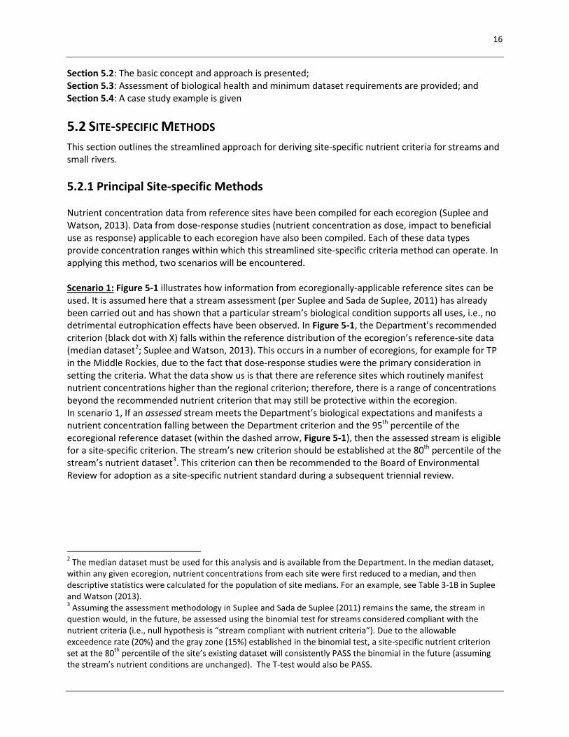
5.2 SITE-SPECIFIC METHODS This section outlines the streamlined approach for deriving site-specific nutrient criteria for streams and small rivers. 5.2.1 Principal Site-specific Methods Nutrient concentration data from reference sites have been compiled for each ecoregion (Suplee and Watson, 2013). Data from dose-response studies (nutrient concentration as dose, impact to beneficial use as response) applicable to each ecoregion have also been compiled. Each of these data types provide concentration ranges within which this streamlined site-specific criteria method can operate. In applying this method, two scenarios will be encountered. Scenario 1: Figure 5-1 illustrates how information from ecoregionally-applicable reference sites can be used. It is assumed here that a stream assessment (per Suplee and Sada de Suplee, 2011) has already been carried out and has shown that a particular stream’s biological condition supports all uses, i.e., no detrimental eutrophication effects have been observed. In Figure 5-1, the Department’s recommended criterion (black dot with X) falls within the reference distribution of the ecoregion’s reference-site data (median dataset2; Suplee and Watson, 2013). This occurs in a number of ecoregions, for example for TP in the Middle Rockies, due to the fact that dose-response studies were the primary consideration in setting the criteria. What the data show us is that there are reference sites which routinely manifest nutrient concentrations higher than the regional criterion; therefore, there is a range of concentrations beyond the recommended nutrient criterion that may still be protective within the ecoregion. In scenario 1, If an assessed stream meets the Department’s biological expectations and manifests a nutrient concentration falling between the Department criterion and the 95th percentile of the ecoregional reference dataset (within the dashed arrow, Figure 5-1), then the assessed stream is eligible for a site-specific criterion. The stream’s new criterion should be established at the 80th percentile of the stream’s nutrient dataset3. This criterion can then be recommended to the Board of Environmental Review for adoption as a site-specific nutrient standard during a subsequent triennial review.
2 The median dataset must be used for this analysis and is available from the Department. In the median dataset, within any given ecoregion, nutrient concentrations from each site were first reduced to a median, and then descriptive statistics were calculated for the population of site medians. For an example, see Table 3-1B in Suplee and Watson (2013). 3 Assuming the assessment methodology in Suplee and Sada de Suplee (2011) remains the same, the stream in question would, in the future, be assessed using the binomial test for streams considered compliant with the nutrient criteria (i.e., null hypothesis is “stream compliant with nutrient criteria”). Due to the allowable exceedence rate (20%) and the gray zone (15%) established in the binomial test, a site-specific nutrient criterion set at the 80th percentile of the site’s existing dataset will consistently PASS the binomial in the future (assuming the stream’s nutrient conditions are unchanged). The T-test would also be PASS.
17
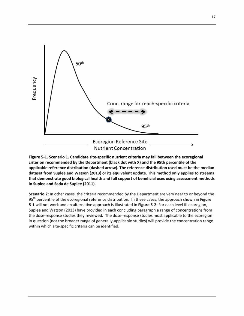
Figure 5-1. Scenario 1. Candidate site-specific nutrient criteria may fall between the ecoregional criterion recommended by the Department (black dot with X) and the 95th percentile of the applicable reference distribution (dashed arrow). The reference distribution used must be the median dataset from Suplee and Watson (2013) or its equivalent update. This method only applies to streams that demonstrate good biological health and full support of beneficial uses using assessment methods in Suplee and Sada de Suplee (2011). Scenario 2: In other cases, the criteria recommended by the Department are very near to or beyond the 95th percentile of the ecoregional reference distribution. In these cases, the approach shown in Figure 5-1 will not work and an alternative approach is illustrated in Figure 5-2. For each level III ecoregion, Suplee and Watson (2013) have provided in each concluding paragraph a range of concentrations from the dose-response studies they reviewed. The dose-response studies most applicable to the ecoregion in question (not the broader range of generally-applicable studies) will provide the concentration range within which site-specific criteria can be identified.
18
Figure 5-2. Scenario 2. Site-specific criteria derivation method for cases where a Department-recommended criterion is near or above the 95th percentile of the ecoregional reference distribution. Candidate site-specific nutrient criteria fall between the criterion recommended by the Department (black dot with X) and the upper range of the values from the dose-response studies specifically applicable to the ecoregion in question (dashed arrow with gray fringe). The dose-response studies must be from Suplee and Watson (2013) or equivalent updates. If an assessed stream meets the Department’s biological expectations but manifests a nutrient concentration above the Department’s criterion, and that criterion is near or above the 95th percentile of the ecoregional reference dataset, then the range of concentrations from the applicable dose-response studies can be reviewed. If the assessed stream’s nutrient concentration at the 80th percentile falls within the range of the regionally-applicable dose-response studies, then that concentration can be used as a site-specific criterion. This criterion can then be recommended to the Board of Environmental Review to be adopted as a site-specific nutrient standard. 5.2.2 Other Methods Recent work in the scientific literature provides a means to develop site-specific criteria on a stream-by-stream basis; the method was specifically developed for western regions of the United States (Olson and Hawkins, 2013). This method uses a geospatially-driven model that considers major environmental factors within a watershed that influence nutrient concentrations in streams (geology, precipitation, soil bulk density, etc.). The Department is using this method to help derive nutrient criteria for an area of the state with few or no reference sites and what appears to be naturally-elevated phosphorus concentrations. It should be pointed out that the method is not for use in the plains region of Montana (Olson and Hawkins, 2013). The Department will consider results provided by others that have used the Olson and Hawkins (2013) method. (Again, this is predicated on the assumption that full biological support is shown in the stream.)
19
However, results from this model will need to be reviewed by the Department on a case-by-case basis. If approved, they can be recommended to the Board of Environmental Review for adoption as site-specific standards. In general, streams whose nutrient concentrations fall outside of the defined ranges in Figures 5-1 and 5-2 are not eligible for this streamlined approach. Rather, methods outlined in Appendix A of the Department’s draft guidance document “Nutrient Standards Implementation Guidance” should be used. There may also be cases where an upstream level IV ecoregion with naturally high nutrient concentrations is influencing the stream in question, and the reach-specific methods in Section 4.0 of Suplee and Watson (2013) may be applicable.
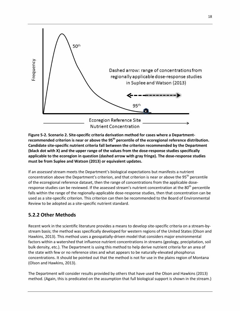
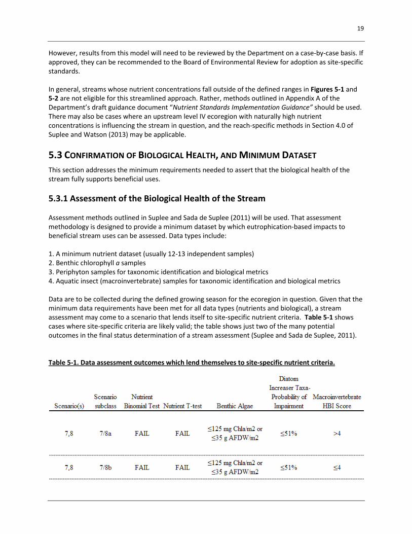
5.3 CONFIRMATION OF BIOLOGICAL HEALTH, AND MINIMUM DATASET This section addresses the minimum requirements needed to assert that the biological health of the stream fully supports beneficial uses. 5.3.1 Assessment of the Biological Health of the Stream Assessment methods outlined in Suplee and Sada de Suplee (2011) will be used. That assessment methodology is designed to provide a minimum dataset by which eutrophication-based impacts to beneficial stream uses can be assessed. Data types include: 1. A minimum nutrient dataset (usually 12-13 independent samples) 2. Benthic chlorophyll a samples 3. Periphyton samples for taxonomic identification and biological metrics 4. Aquatic insect (macroinvertebrate) samples for taxonomic identification and biological metrics Data are to be collected during the defined growing season for the ecoregion in question. Given that the minimum data requirements have been met for all data types (nutrients and biological), a stream assessment may come to a scenario that lends itself to site-specific nutrient criteria. Table 5-1 shows cases where site-specific criteria are likely valid; the table shows just two of the many potential outcomes in the final status determination of a stream assessment (Suplee and Sada de Suplee, 2011). Table 5-1. Data assessment outcomes which lend themselves to site-specific nutrient criteria.

20
In Table 5-1, which applies to western Montana streams, it has been found that an assessed stream’s nutrients are elevated and fail both statistical tests (the binomial, which looks as the proportion of observations above the criterion, and the t-test, which addresses the dataset average and the presence of high outliers). Note however that the biological signals are all or nearly all acceptable; benthic algal biomass is below the threshold, diatom metrics (where applicable) show a low probability of nutrient impairment, and the macroinvertebrate-based HBI metric is acceptable since it is < 4 (at least for scenario subclass 7/8b), meaning water quality is very good (Hilsenhoff, 1987). Of the two cases shown, subclass 7/8a is less clear due to the elevated HBI score and additional data collection would be warranted before site-specific criteria are developed. For prairie streams, see scenarios 5 and 7, part 2 (Suplee and Sada de Suplee, 2011) as they are equivalent to those in Table 5-1. 5.3.2 Dataset Minimum All data collection must follow Department SOPs (e.g., DEQ, 2011a; DEQ, 2011b; DEQ, 2012). Dataset minimums for a stream assessment are defined in Suplee and Sada de Suplee (2011). For the purposes of developing site-specific nutrient criteria via this process, the dataset needs to have been collected for three years (though not necessarily contiguously) for all of the data types required in Suplee and Sada de Suplee (2011). For western Montana streams, this would be nutrients, benthic chlorophyll a, diatoms (where applicable), and macroinvertebrates. If the dataset minimums to complete a stream assessment were achieved after just two years of data collection (which is common), a complete third year of data must be collected as well. For prairie streams, data types should include nutrients, measurement of dissolved oxygen (5 continuous days at a minimum, during summer), diatoms, and visual assessment of aquatic plant densities (DEQ 2011a), for a minimum of three years. The complete, three-year dataset must be taken through the assessment data matrix. In some cases the additional year may change the initial outcome and it may result that the stream no longer comes to the scenarios shown in Table 5-1 and site-specific criteria are not warranted. However if the assessed stream again arrives to the scenarios in Table 5-1, site-specific nutrient criteria are likely warranted and the approaches outlined in Section 5.2 may be applied. 5.3.3 Consideration of the Other Nutrient Where a site-specific criterion is warranted for a nutrient elevated above the Department’s ecoregion- based criteria, consideration must be given to the other nutrient in the stream (N vs. P, and vise-versa). For example, a stream manifesting good biological health but elevated P concentrations may very likely be N limited, and should be maintained so. If N limitation were alleviated, there is a high likelihood that the biological health of the stream would be impacted. The Redfield ratio (Redfield, 1958) will be used as a general guide for establishing which nutrient limits (ratio < 6, N limits; ratio > 10, P limits) and for establishing the final concentration of the other nutrient. What the updated criterion for the non-elevated nutrient should be needs to be determined on a case-by-case basis in conjunction with the Department. A first-cut approximation would be roughly 75% of the established ecoregional criterion concentration. In some cases, both N and P will be elevated above the Department’s recommended criteria. In such cases each nutrient should be evaluated per methods in Section 2.0 and it may result that site-specific

21
criteria for both N and P will be higher than the Department’s values. In such cases factors other than nutrients are likely limiting nutrient effects in the stream.
5.4 CASE-STUDY EXAMPLE The following is a case which lends itself to site-specific nutrient criteria. 5.4.1 Data Summary for Stream X (in Middle Rockies Ecoregion) Years of data: 3 (2004, 2011, 2012) Number of Nutrient Samples: 12-14 (meets minimum) Average Total Phosphorus (TP) Concentration: 35 µg/L Average Total Nitrogen (TN) Concentration: 40 µg/L Benthic Chlorophyll a Samples: 3 (each comprised of 11 sub-replicates) (meets minimum) Diatom Metric Samples: Not applicable (Department has no validated diatom-based metrics for the Middle Rockies ecoregion at this time) Macroinvertebrates Samples: 3 (meets minimum) 5.4.2 The Assessment of Stream X The applicable criteria for the Middle Rockies are 30 µg TP/L and 300 µg TN/L (Suplee and Watson, 2013). Data for stream X were evaluated and TN was found to be quite low (average = 40 µg/L), well below the recommended ecoregional criterion of 300 µg/L. However TP averaged 35 µg/L and was above the ecoregional criterion of 30 µg/L. All biological indicators were found to be acceptable; the data fit scenario subclass7/8b in Table 5-1. In additional, other aspects of the data were considered. The macroinvertebrate O/E scores were reviewed to see if they were above 1.04 (none were). The benthic chlorophyll a concentrations were not only below the threshold they were very low (<< 50 mg Chla/m2), as was algal AFDM. Nitrate concentrations were also evaluated, and all concentrations were very low. 5.4.3 Site-specific Criteria Derivation for Stream X using the Streamlined Approach The Department’s recommended criterion for the Middle Rockies ecoregion (where stream X is located) is 30 µg TP/L; this value matches the 82nd percentile of the Middle Rockies’ reference data (median dataset; Suplee and Watson, 2013). The TP concentration at the 80th percentile of stream X’s dataset is 42 µg TP/L, a concentration equal to the 89th percentile in the Middle Rockies reference dataset. Therefore, stream X fits scenario 1 (Figure 5-1) because its site-specific TP value (42 µg/L) falls between the Department’s recommended criterion and the 95th percentile of the Middle Rockies reference dataset. Stream X’s new criterion (42 µg TP/L) is not too far above the Department’s criterion, so a large
4 O/E scores decline from an ideal score of 1.0 due to impacts from a variety of stressors (excess sediment, heavy metals, elevated temperatures, etc.). However it is not uncommon to see scores > 1.0. These indicate the stream has more species of macroinvertebrates than the model is expecting to see for the region. Essentially, slightly elevated nutrient levels have led to a less austere environment and more species can exist than is normally seen. For this reason O/E scores > 1.0 can be indicative of nutrient enrichment above reference. When nutrient enrichment becomes excessive, O/E scores again drop below 1.
22
reduction in the stream’s TN criterion is not warranted. But it is prudent to set the TN lower than 300, to 250 µg TN/L (which is at the 97th percentile of the Middle Rockies reference distribution). This maintains a Redfield ratio of < 6 which should help maintain N limitation. The site specific criteria would be 42 µg TP/L and 250 µg TN/L, applicable during the growing season for the Middle Rockies (July1-Sept 30).
6.0 GUIDELINES FOR DEVELOPING SITE-SPECIFIC NUMERIC NUTRIENT CRITERIA VIA WATER QUALITY MODELING, AND THE RELATION OF THESE CRITERIA TO INDIVIDUAL NUTRIENT STANDARDS VARIANCES
Circumstances may arise where, for a specific discharger, it may not make sense to move to the new, lower general variance concentrations at the time the Department updates them during a triennial standards review. Similarly, it may not make sense for a discharger to upgrade to one of the nutrient reduction steps (see Section 2.0 of this document) that have been defined for the 3 permit cycles subsequent to the initial treatment requirements (e.g., 1 mg TP/L and 10 mg TN/L) defined in statue at §75-5-313 (5)(b), MCA. In some cases a permittee may be able to demonstrate, using water quality modeling and reach-specific data, that greater emphasis on reducing one nutrient (the target nutrient) will achieve the same desired water-quality conditions as can be achieved by emphasizing reduction of both nutrients. Requiring a point source discharger to immediately install sophisticated nutrient-removal technologies to reduce the non-target nutrient to levels more stringent than what is in statute at §75-5-313(5)(b), MCA may not be the most prudent nutrient control expenditure, and would cause the discharger to incur unnecessary economic expense. Since this can be interpreted as a form of economic impact, sensu §75-5-313(1), MCA, these situations are appropriately addressed by individual variances. If such a case can be demonstrated to the satisfaction of the Department, then a permittee can apply for an individual variance which will include discharger-specific limits reflecting the highest attainable condition for the receiving water rather than limits based on any new general variance concentration. The demonstration must consider effects on the downstream waterbody including effects from the non-target nutrient; if the downstream waterbody will be impacted by the facility, some additional level of reduction on the target and/or non-target nutrient (beyond that required to protect beneficial uses in the receiving waterbody)will be necessary or the individual variance may not be granted. In addition, the permittee is required to provide monitoring water-quality data that can be used to determine if the justification for less stringent effluent limits continues to hold true (i.e., status monitoring is required). Because status can change, for example due to substantive nonpoint source cleanups upstream of the discharger, status monitoring by the discharger is required. The purpose of Section 6.0 is to provide guidelines for the types of information the Department would need to evaluate in order to permit a discharger to remain at treatment levels less stringent than any general variance requirements as defined in Section 2.0 of this document.

23
6.1 MECHANISTIC AND EMPIRICAL MODELING APPROACHES FOR ESTABLISHING INDIVIDUAL VARIANCES AND (POTENTIALLY) REACH-SPECIFIC NUTRIENT STANDARDS Two approaches may be used to establish that upgrading a wastewater facility to updated general variance levels would not result in material progress towards attaining defined water-quality endpoints and beneficial use support:
1. Simulations based on mechanistic computer models 2. Demonstration of use support based on empirical data
Whichever approach is selected—and in fact both approaches can be pursued simultaneously—the Department will require a 2-year biological characterization of the reach in question. A solid understanding of the biological status existing under the current level of water quality is required. Factors (both natural and human-caused) independent of nutrient concentrations can influence biological integrity and need to be understood. The biological characterization will change from case to case, but will normally involve collection of diatoms, macroinvertebrates, benthic and phytoplankton algae density, and critical physical and chemical parameters that influence these. See Section 2.0 Appendix A for an example of the types of biological data and the rationale for each. The following provides further detail on the two modeling approaches bulleted above. Simulation Based on Mechanistic Computer Models. The Department will consider mechanistic model results that demonstrate that the lowering of one nutrient (e.g., TP) without the lowering (or with less lowering) of the other would achieve essentially the same water quality endpoint (i.e., equivalent movement towards the water quality goal), subject to Department approval of the model and the model’s parameterization. Modeled endpoints may include changes in water quality (pH, dissolved oxygen, etc.), and benthic and phytoplankton algae density. Mechanistic models must be supported by data from a Department-approved study design that includes characterization of the chemical, biological, and hydrological conditions of the study reach during a lower-than-average baseflow condition. Data collection should follow Department SOPs. The Department encourages the use of the QUAL2K model (Chapra et al., 2010) but may consider results from other water quality models as well. Modeled nutrient reduction scenarios can vary, but scenarios based on the five treatment levels described in Falk et al. (2011)—which represent steps in biological nutrient removal technologies—are encouraged by the Department. The Department will consider nitrogen and phosphorus independently in this analysis. The state of the art in computer water quality/algal growth modeling is such that nutrient co-limitation and community interaction of river flora is poorly simulated (or is not simulated at all). Models usually treat algal growth dynamics in streams and rivers as though the algae were a monoculture (which is not the case). Because of the uncertainties in model simulations, the Department will require monitoring (per NEW RULE I [3]) for dischargers that are permitted to depart from general variance concentration requirements based on a mechanistic model. The intent of the monitoring is to corroborate (or refute) the computer simulated results. At a minimum, growing season benthic-algae sampling will be required

24
for a reach of the river downstream of the permittee’s mixing zone, to be established in coordination with the Department. If the base numeric nutrient standard for the river in question was developed based on another water quality endpoint (for example, pH), then data collection must also include that parameter. If the collected data and the computer modeling results corroborate one another, then a reach-specific base numeric nutrient standard may be in order. Any reach-specific nutrient standard so determined may be adopted by the Board of Environmental Review under its rulemaking authority in §75-5-301(2), MCA. Demonstration of Use Support Based on Empirical Data. Permittees may begin at any time to collect nutrient concentration, benthic and phytoplankton algae, and other biological and water quality data in the receiving waterbody downstream of their mixing zone. In cases where the Department’s base numeric nutrient standards for the waterbody were developed using a specific water quality endpoint (for example, pH), data collection must include that parameter. Data collection shall follow Department SOPs. Permittees are strongly encouraged to coordinate with the Department on study design and data collection protocols upfront, to assure that the data will be acceptable to the Department when the time comes for evaluating the outcomes. For example, it has been shown that chlorination of effluent can, in some cases, mute the effects of nutrients for some distance downstream (Gammons et al., 2010); this would need to be accounted for in any study design. Subject to Department approval, these data may be used to demonstrate that remaining at the previous general-variance treatment level (assumed here to have been achieved by the permittee) was adequate to support beneficial uses of the waterbody. If the collected data conclusively indicate that beneficial uses of the waterbody are fully supported, then reach-specific base numeric nutrient standards may be in order. Any reach-specific nutrient standards so determined may be adopted by the Board of Environmental Review under its rulemaking authority in §75-5-301(2), MCA. An example of an empirical approach to developing reach-specific nutrient criteria is provided in Section 2.0 of Appendix A.
6.2 PROTECTION OF DOWNSTREAM BENEFICIAL USES Any reach-specific criteria developed for a receiving stream using a mechanistic or empirical model will also need to protect downstream beneficial uses. “How far downstream” is a consideration which will vary from case-to-case; an example is provided in Sections 2.7 and 4.0 of Appendix A. Mechanistic models have very clear advantages over empirical models for running hypothetical scenarios and assessing potential downstream impacts, however a mechanistic model will normally be more expensive to complete. A budget estimate for a mechanistic and an empirical model is provided in Section 6.0 of Appendix A. If it results that modeling (of either type) has shown that beneficial uses of the assessed reach can be protected with site-specific criteria, but a downstream reach will be negatively impacted by the higher concentrations of one (or both) nutrients, then the Department will require treatment levels which will support the uses in the downstream waterbody or it will not grant the individual variance.
6.3. UNWARRANTED COST AND ECONOMIC IMPACT In order to satisfy the economic impact component of an individual variance (§75-5-313[2], MCA) permittees must provide the Department approximate estimates of the capital costs, and operations and maintenance costs, which would have been expended in order to upgrade the facility to the new general variance concentrations. The intent is to demonstrate that there were substantial savings in capital costs, materials, fuel, and energy by opting not to upgrade the facility. The permittee can compare the cost saved to the MHI of the community, similar to what is done for determining substantial and widespread economic impacts (see steps 1 through 5, Section 2.2); however, the
25
Department wants to make clear that no specific percent of MHI needs to be realized in order for this aspect of the analysis to be satisfied. Permittees are encouraged to work with the Department’s economist when carrying out this analysis (Jeff Blend or his successor). Capital costs saved would not include design-related work and overhead. Operations and maintenance cost saved should be estimates of fuel and/or electrical consumption, and other materials (e.g., chemicals). Permittees are not required to carry out a complex analysis comparing the relative economic or social value of protecting one resource (the stream or river) vs. another (e.g., air quality) and then trying to quantify the relative savings. Rather, the Department wants a straight-forward quantification of cost savings associated with the key factors of concern (capitol costs, fuel and electrical consumption, and routine materials such as chemical additions).
6.4 DEPARTMENT ADOPTION AND PERIODIC REVIEW OF THE INDIVIDUAL VARIANCE Nutrient concentrations in the draft individual variance would be based on the results of modeling and the assessment of downstream use protection as described above. Individual variances approved by the Department become effective and may be incorporated into a permit only after a public hearing and adoption by the Department (§75-5-313[4], MCA). Status monitoring of the receiving stream and the affected downstream waterbody will be used to evaluate the individual variance justification going forward. For example: model results have shown that a large reduction of phosphorus by the permittee would render the receiving stream P-limited and in full support of beneficial uses, without a reduction in nitrogen. At the same time, nonpoint contributions of nitrogen to the downstream waterbody of concern are presently large enough that a substantial reduction of nitrogen load by the permittee would have had little or no beneficial effect. As a result, the permittee’s individual variance reflects a low TP concentration and a TN concentration of 10 mg/L. If in the next ten years (of the twenty year variance period) nonpoint sources cleanup sufficiently that the 10 mg TN/L concentration has become a sizeable proportion of the downstream nitrogen load and reduction of that load would benefit the stream, then the justification for the 10 mg TN/L will have changed. Any updated individual variance would reflect a lower TN concentration. As before, modeling could be used to help derive the updated TN concentration.
7.0 REFERENCES
Chapra, S.C., Pelletier, G.J., and Tao, H. 2010. QUAL2K: A Modeling Framework for Simulating River and Stream Water Quality, Version 2.11: Documentation and Users Manual.
DEQ (Department of Environmental Quality), 2011a. Sample Collection and Laboratory Analysis of
Chlorophyll-a Standards Operating Procedure. WQPBWQM-011 Version 6.0, Available at: http://deq.mt.gov/wqinfo/qaprogram/sops.mcpx
DEQ (Department of Environmental Quality), 2011b. Periphyton Standard Operating Procedure.
WQPBWQM-010, Available at: http://deq.mt.gov/wqinfo/qaprogram/sops.mcpx DEQ (Department of Environmental Quality), 2012. Sample Collection, Sorting, Taxonomic Identification,
and Analysis of Benthic Macroinvertebrate Communities Standard Operating Procedure. WQPBWQM-009 Revision 3, Available at: http://deq.mt.gov/wqinfo/qaprogram/sops.mcpx

26
Falk, M.W., J.B. Neethling, and D.J. Reardon, 2011. Striking a Balance between Wastewater Treatment Nutrient Removal and Sustainability. Water Environment Research Foundation, document NUTR1R06n, IWA Publishing, London, UK.
Gammons, C.H., J.N. Babcock, S.R. Parker, and S.R. Poulson, 2010. Diel Cycling and Stable Isotopes of
Dissolved Oxygen, Dissolved Inorganic Carbon, and Nitrogenous Species in a Stream Receiving Treated Municipal Sewage. Chemical Geology, doi 10.1016/j.chemgeo.2010.07.006.
Hilsenhoff, W. L. 1987. An Improved Biotic Index of Organic Stream Pollution. Great Lakes Entomologist.
20(1): 31-39. Olson, J.R., and C.P. Hawkins. 2013. Developing Site-specific Nutrient Criteria from Empirical Models.
Freshwater Science 32(3): 719-740. Redfield, A. C. 1958. The biological control of chemical factors in the environment. Am. Sci. 46: 205-
221. Suplee, M.W., and R. Sada de Suplee, 2011. Assessment Methodology for Determining Wadeable
Stream Impairment Due to Excess Nitrogen and Phosphorus Levels. Helena, MT: Montana Department of Environmental Quality, 70 p. Available at: http://deq.mt.gov/wqinfo/qaprogram/sops.mcpx
Suplee, M.W. and V. Watson, 2013. Scientific and Technical Basis of the Numeric Nutrient Criteria for
Montana’s Wadeable Streams and Rivers: Update 1. Helena, MT: Montana Department of Environmental Quality, 125 p. Available at: http://deq.mt.gov/wqinfo/standards/NumericNutrientCriteria.mcpx
U.S. Environmental Protection Agency. 1995. Interim Economics Guidance for Water Quality Standards -
Workbook. U.S. Environmental Protection Agency. Report EPA-823-B-95-002.

27
APPENDIX A: RECOMMENDATIONS FOR SAMPLING AND MODELING THE EAST GALLATIN RIVER TO ACCOMPLISH MULTIPLE OBJECTIVES
1.0 Background The Department indicated in its draft numeric nutrient standards rule package that a person may collect and analyze water quality and biological data along a reach of stream or river to determine if reach-specific numeric nutrient criteria different from those of the Department are warranted. A draft proposal of this type was provided to the Department in July 2012 for the East Gallatin River (HDR Engineering, 2012)5. The Sampling and Analysis Plan (SAP) provided to the Department in July 2012 (HDR Engineering, 2012) is based on sites that were sampled in 2009-2010 for the purpose of determining flow-stage relationships in the East Gallatin River. Building on those sites, the following are recommendations for an optimized study design which can be used to develop reach-specific nitrogen and phosphorus criteria for the East Gallatin River. It is hoped that this document may also serve as a blueprint for similar work that may be carried out on other Montana rivers or streams. The Department already has a public-reviewed and finalized assessment methodology for determining when a stream reach is impaired by excess nitrogen and phosphorus (Suplee and Sada de Suplee, 2011). However, that assessment methodology was designed to be a minimum data method and was not intended to be sufficient for deriving reach-specific criteria. Therefore, the reader will find that methods recommended below are more data intensive than those needed to complete an assessment via the assessment methodology.
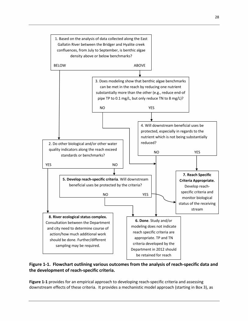
1.1 Design and Possible Outcomes of the Investigation The East Gallatin River is an excellent case study in which to explore several variations on the development of reach-specific criteria. These variations include: 1. The case where a stream reach may have natural factors (e.g. high turbidity, cold temperature, etc.) that suppress benthic algae growth, and therefore reach-specific criteria are appropriate; 2. The case where benthic algae is found to be above nuisance levels, but modeling shows the algae problem can be addressed by focusing on the reduction of one nutrient more than the other; or 3. The case where reach-specific numeric nutrient criteria for a reach of the East Gallatin River are appropriate, but consideration of downstream beneficial uses precludes their application. Figure 1-1 below forms the basis for the recommendations in the rest of this document.
5 It should be noted that the Department has developed reach-specific criteria for the East Gallatin River using approaches somewhat different than those provided here. See Section 4.0 in Suplee and Watson (2012).
28
Figure 1-1. Flowchart outlining various outcomes from the analysis of reach-specific data and the development of reach-specific criteria. Figure 1-1 provides for an empirical approach to developing reach-specific criteria and assessing downstream effects of these criteria. It provides a mechanistic model approach (starting in Box 3), as
1. Based on the analysis of data collected along the East Gallatin River between the Bridger and Hyalite creek confluences, from July to September, is benthic algae
density above or below benchmarks?
BELOW ABOVE
6. Done. Study and/or modeling does not indicate reach specific criteria are appropriate. TP and TN
criteria developed by the Department in 2012 should
be retained for reach
8. River ecological status complex. Consultation between the Department and city need to determine course of
action/how much additional work should be done. Further/different
sampling may be required.
2. Do other biological and/or other water quality indicators along the reach exceed
standards or benchmarks?
YES NO
5. Develop reach-specific criteria. Will downstream beneficial uses be protected by the criteria?
NO YES
3. Does modeling show that benthic algae benchmarks can be met in the reach by reducing one nutrient
substantially more than the other (e.g., reduce end-of pipe TP to 0.1 mg/L, but only reduce TN to 8 mg/L)?
NO YES
4. Will downstream beneficial uses be protected, especially in regards to the nutrient which is not being substantially reduced?
NO YES
7. Reach Specific Criteria Appropriate.
Develop reach-specific criteria and monitor biological
status of the receiving stream
29
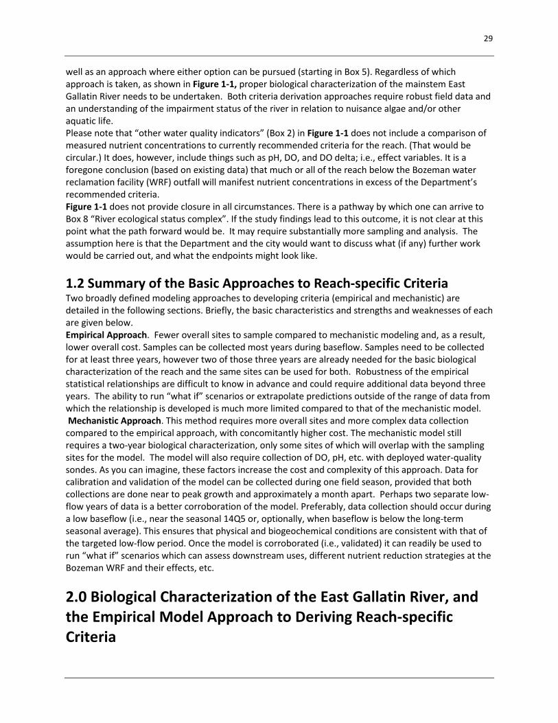
well as an approach where either option can be pursued (starting in Box 5). Regardless of which approach is taken, as shown in Figure 1-1, proper biological characterization of the mainstem East Gallatin River needs to be undertaken. Both criteria derivation approaches require robust field data and an understanding of the impairment status of the river in relation to nuisance algae and/or other aquatic life. Please note that “other water quality indicators” (Box 2) in Figure 1-1 does not include a comparison of measured nutrient concentrations to currently recommended criteria for the reach. (That would be circular.) It does, however, include things such as pH, DO, and DO delta; i.e., effect variables. It is a foregone conclusion (based on existing data) that much or all of the reach below the Bozeman water reclamation facility (WRF) outfall will manifest nutrient concentrations in excess of the Department’s recommended criteria. Figure 1-1 does not provide closure in all circumstances. There is a pathway by which one can arrive to Box 8 “River ecological status complex”. If the study findings lead to this outcome, it is not clear at this point what the path forward would be. It may require substantially more sampling and analysis. The assumption here is that the Department and the city would want to discuss what (if any) further work would be carried out, and what the endpoints might look like.
1.2 Summary of the Basic Approaches to Reach-specific Criteria Two broadly defined modeling approaches to developing criteria (empirical and mechanistic) are detailed in the following sections. Briefly, the basic characteristics and strengths and weaknesses of each are given below. Empirical Approach. Fewer overall sites to sample compared to mechanistic modeling and, as a result, lower overall cost. Samples can be collected most years during baseflow. Samples need to be collected for at least three years, however two of those three years are already needed for the basic biological characterization of the reach and the same sites can be used for both. Robustness of the empirical statistical relationships are difficult to know in advance and could require additional data beyond three years. The ability to run “what if” scenarios or extrapolate predictions outside of the range of data from which the relationship is developed is much more limited compared to that of the mechanistic model. Mechanistic Approach. This method requires more overall sites and more complex data collection compared to the empirical approach, with concomitantly higher cost. The mechanistic model still requires a two-year biological characterization, only some sites of which will overlap with the sampling sites for the model. The model will also require collection of DO, pH, etc. with deployed water-quality sondes. As you can imagine, these factors increase the cost and complexity of this approach. Data for calibration and validation of the model can be collected during one field season, provided that both collections are done near to peak growth and approximately a month apart. Perhaps two separate low-flow years of data is a better corroboration of the model. Preferably, data collection should occur during a low baseflow (i.e., near the seasonal 14Q5 or, optionally, when baseflow is below the long-term seasonal average). This ensures that physical and biogeochemical conditions are consistent with that of the targeted low-flow period. Once the model is corroborated (i.e., validated) it can readily be used to run “what if” scenarios which can assess downstream uses, different nutrient reduction strategies at the Bozeman WRF and their effects, etc.
2.0 Biological Characterization of the East Gallatin River, and the Empirical Model Approach to Deriving Reach-specific Criteria

30
Objective 1: Determine the current biological condition of the reach of the East Gallatin River between the Bridger Creek and West Gallatin River confluences during the growing season (summer and early fall) and compare the results to standards and benchmarks used to assess stream eutrophication. 2.1 Detailed Consideration of the Objective 1 The following questions are designed to address objective 1 given above: In the wadeable regions of the East Gallatin River between the Bridger Creek and West Gallatin River confluences, during the July 20 to September 30 period, what: (a) are the average benthic algae densities (quantified as chlorophyll a and ash free dry mass, per m2)? (b) is the areal coverage and thickness of benthic algae and macrophytes (based on standardized visual assessment methods)? (c) is the range and central tendency of specified macroinvertebrate metric scores (MT Hilsenhoff Biotic Index, O/E, and EPT taxa richness)? (d) is the range and central tendency of specified diatom metric scores (WEMAP MVI and WEMAP WA TN)? (e) are the dissolved oxygen concentrations and pH compared to state standards, and what is the dissolved oxygen delta (daily maximum minus the daily minimum)? (f) are the concentrations of nitrogen and phosphorus (total and soluble) and total suspended solids? (g) is the stream temperature, and incoming light intensity( in PAR units, e.g., µmol quanta/m2∙s)? (h) are the concentrations of herbicides which are frequently used in the watershed? Note in the question at the start of Section 2.1 the dates during which data collection should occur (July 20 to the end of September). These dates were based on the Middle Rockies growing season (Suplee et al., 2007), and the fact that in the East Gallatin River the first three weeks of July have considerably higher flows compared to August and September (shown in dark gray, Table 2-1). Commencing July sampling after July 20th will generally exclude the higher flows and lead to data collection during base flow conditions more consistent with August and September. Sampling could extend into the first two weeks of October, if temperatures remain moderate and base flow conditions remain reasonably stable (Suplee and Sada de Suplee, 2011).

31
To further address the questions posed at the start of Section 2.1, it will be necessary to measure a number of physico-chemical parameters; the rationale for measuring each of these is described below. Biological parameters specified in the questions above were selected because they are known to be directly influenced by or significantly correlate with lotic nutrient concentrations. The Department has established benchmarks for most of the physic-chemical and biological variables, and East Gallatin River data can be compared against these (DEQ-7, 2012; Suplee and Sada de Suplee, 2010). Benthic algae densities (chlorophyll a [Chla] and ash free dry mass [AFDM] per m2). Based on work in the Clark Fork River, statewide public opinion surveys, and a whole-stream dose-response study, the Department is using average Chla levels of 125 to 150 mg/m2 and 35 g AFDM/m2 as harm-to-use thresholds for western Montana rivers and streams (Dodds et al., 1997; Suplee et al., 2009; Suplee and Sada de Suplee, 2011). Algae densities above these levels impact the recreation and aquatic life uses. The Department also has standard visual assessment methods to asses algal and macrophyte density at a coarser scale (WQPBWQM-011, 2011). The general composition, amount, color, and condition of aquatic plants are visually assessed in the field using the Aquatic Plant Visual Assessment Form. This information helps describe the health and productivity of the aquatic ecosystem, records nuisance aquatic plant problems, documents changes in the plant community over time, and can be used to help corroborate the quantitative Chla results.
Day ofmonth Jan Feb Mar Apr May Jun Jul Aug Sep Oct Nov Dec
1 42 47 45 118 283 433 164 52 43 40 55 472 44 43 44 128 267 441 155 51 42 41 55 473 44 42 46 124 268 453 147 53 39 42 57 474 41 43 48 112 297 433 142 53 37 44 56 475 43 44 47 121 295 418 141 51 39 48 55 476 43 47 46 148 328 425 130 52 42 50 53 477 41 44 46 139 364 479 124 51 43 51 55 468 46 44 52 140 379 461 118 52 41 51 62 439 44 42 54 149 376 440 108 54 43 52 60 4310 42 42 56 157 380 443 102 52 50 52 56 4411 41 42 58 155 373 513 101 49 45 52 56 4612 42 42 70 164 373 501 97 46 41 53 56 4613 43 42 88 182 377 465 94 45 42 52 57 4514 44 42 88 218 404 436 90 45 42 52 56 4515 43 41 80 232 439 420 84 47 43 55 52 4516 42 41 80 212 442 404 81 44 42 59 55 4317 44 41 81 229 464 390 78 44 44 61 54 4218 46 41 86 239 484 359 75 47 45 59 53 4119 51 42 89 235 509 335 73 46 44 59 53 4320 48 40 88 231 528 310 68 42 44 66 52 4421 47 41 93 254 523 299 66 41 46 63 49 4522 44 41 94 279 505 277 66 41 47 58 47 4423 44 41 94 324 495 264 67 45 48 56 48 4624 44 41 90 315 500 247 62 43 49 56 46 4425 43 41 89 290 615 237 63 41 46 57 48 4526 43 42 95 293 540 228 64 41 43 55 50 4627 47 43 93 270 502 209 63 39 42 55 48 4428 46 43 95 266 475 195 61 39 42 55 47 4429 44 41 91 274 490 183 55 41 42 57 46 4630 45 97 295 466 175 51 41 44 57 47 4431 43 104 444 50 43 56 43
Table 2-1. Discharge, ft3/sec for USGS Station 06048700 "East Gallatin River at Bozeman, Mont.". Mean of daily values for 10 years of record (calculation period 2001-10-01 to 2011-09-30).
32
Macroinvertebrate metrics. The Hilsenhoff Biotic Index (HBI) is included as part of the Department’s current eutrophication assessment methodology (see Suplee and Sada de Suplee, 2011). The HBI index was designed to assess biological impacts caused by organic enrichment and eutrophication (Hilsenhoff, 1987). The Department considers HBI scores in the Middle Rockies > 4.0 to indicate an impact to aquatic life (Suplee and Sada de Suplee, 2011). Two other metrics, O/E and EPT richness, were considered during the development of the eutrophication assessment methodology since both metrics correlated significantly to nutrient concentrations (Tetra Tech, 2010); however, for simplicity, only the HBI was retained in that methodology. Nevertheless, it would be of value to include these metrics in this study. The O/E metric evaluates the taxa diversity that was actually Observed compared to an Expected taxa diversity for the location where the sample was collected. The Department uses an O/E ratio of 1.0 to 0.9 as un-impacted; ≤ 0.9 is the harm threshold (i.e., loss of 10% of species). Modest stream nutrient enrichment can actually cause the metric to be > 1.0. A Bray-Curtis Index should be calculated to accompany the O/E to help interpret counterintuitive O/E scores (WQPBWQM-009, 2012). The EPT richness metric was part of older DEQ protocols and has application to intermountain valley and foothill streams. EPT richness values > 14 are considered healthy and this value will decline with water quality impacts (Bukantis, 1998). Diatom metrics. The Department currently addresses nutrient impacts using increaser diatom taxa metrics which were developed using discriminant function analysis (Bahls et al., 2008, Teply, 2010a and 2010b; Suplee and Sada de Suplee, 2011). Currently there is no calibrated and validated model for the ecoregion in which the East Gallatin River resides (the Department hopes to have such a metric in a year or so). Therefore, two diatom metrics are recommended (one for TN, one for TP) which were developed by others and which correlate closely with stream nutrient concentrations in Montana (Tetra Tech, 2010). The metrics are WEMAP WA TN (for TN) and WMAP MVI (for TP); each was developed from work in the Western Environmental Monitoring and Assessment Program (EMAP) of the early 2000s. Results that differ largely from the regression line shown in Tetra Tech (2010) might suggest a stream with characteristics different from the Middle Rockies norm; for example, a WEMAP MVI diatom score of 1.5 associated with a TP concentration of 0.25 mg/L would be well outside the expected pattern (one would expect a score closer to 3)(Tetra Tech, 2010). Dissolved oxygen, pH. Standards for dissolved oxygen (DO) and pH for a B-1 waterbody are established in state law (DEQ-7 October, 2012). DO and pH have been linked to elevated nutrient concentrations (Stevenson et al., 2012), making them good parameters to measure. But the Department has frequently observed that DO minima are not found to be out of compliance in heavily eutrophied streams, at least during summer, due to stream re-aeration. However, punctuated DO problems can occur in fall when the built-up algae senesce en masse (Suplee and Sada de Suplee, 2011). Therefore, in addition to state-adopted DO standards, the Department uses DO delta (daily maximum minus the daily minimum) of 5.3 as a benchmark for excessive plant productivity and respiration in streams (see Appendix C.2, Suplee and Sada de Suplee, 2011). Others have found DO delta to be valuable in assessing eutrophication in northern rivers, and recommend a benchmark of 5.0 (Minnesota Pollution Control Agency, 2010). Concentration of nitrogen and phosphorus (total and soluble), total suspended solids, temperature, incoming light intensity, and herbicide concentrations. These water quality parameters are critical for the development of empirical relationships between algae density and nutrient concentrations. Variables that influence light levels are particularly important for algal growth rates. Light measurements can include PAR near the stream bottom, or (as a possible surrogate) measurements of canopy density above the water’s surface. Temperature alters the growth rates of stream algae. In addition, stream samples for herbicides which have historically been used in the basin should be
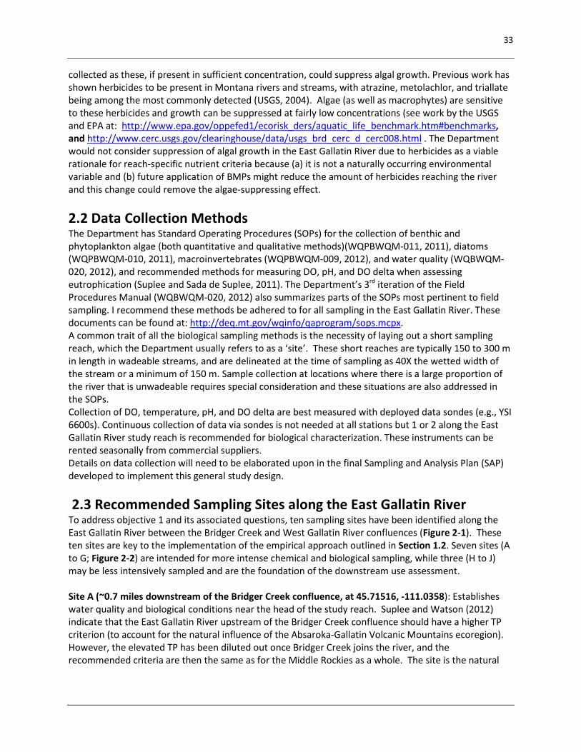
33
collected as these, if present in sufficient concentration, could suppress algal growth. Previous work has shown herbicides to be present in Montana rivers and streams, with atrazine, metolachlor, and triallate being among the most commonly detected (USGS, 2004). Algae (as well as macrophytes) are sensitive to these herbicides and growth can be suppressed at fairly low concentrations (see work by the USGS and EPA at: http://www.epa.gov/oppefed1/ecorisk_ders/aquatic_life_benchmark.htm#benchmarks, and http://www.cerc.usgs.gov/clearinghouse/data/usgs_brd_cerc_d_cerc008.html . The Department would not consider suppression of algal growth in the East Gallatin River due to herbicides as a viable rationale for reach-specific nutrient criteria because (a) it is not a naturally occurring environmental variable and (b) future application of BMPs might reduce the amount of herbicides reaching the river and this change could remove the algae-suppressing effect.
2.2 Data Collection Methods The Department has Standard Operating Procedures (SOPs) for the collection of benthic and phytoplankton algae (both quantitative and qualitative methods)(WQPBWQM-011, 2011), diatoms (WQPBWQM-010, 2011), macroinvertebrates (WQPBWQM-009, 2012), and water quality (WQBWQM-020, 2012), and recommended methods for measuring DO, pH, and DO delta when assessing eutrophication (Suplee and Sada de Suplee, 2011). The Department’s 3rd iteration of the Field Procedures Manual (WQBWQM-020, 2012) also summarizes parts of the SOPs most pertinent to field sampling. I recommend these methods be adhered to for all sampling in the East Gallatin River. These documents can be found at: http://deq.mt.gov/wqinfo/qaprogram/sops.mcpx. A common trait of all the biological sampling methods is the necessity of laying out a short sampling reach, which the Department usually refers to as a ‘site’. These short reaches are typically 150 to 300 m in length in wadeable streams, and are delineated at the time of sampling as 40X the wetted width of the stream or a minimum of 150 m. Sample collection at locations where there is a large proportion of the river that is unwadeable requires special consideration and these situations are also addressed in the SOPs. Collection of DO, temperature, pH, and DO delta are best measured with deployed data sondes (e.g., YSI 6600s). Continuous collection of data via sondes is not needed at all stations but 1 or 2 along the East Gallatin River study reach is recommended for biological characterization. These instruments can be rented seasonally from commercial suppliers. Details on data collection will need to be elaborated upon in the final Sampling and Analysis Plan (SAP) developed to implement this general study design.
2.3 Recommended Sampling Sites along the East Gallatin River To address objective 1 and its associated questions, ten sampling sites have been identified along the East Gallatin River between the Bridger Creek and West Gallatin River confluences (Figure 2-1). These ten sites are key to the implementation of the empirical approach outlined in Section 1.2. Seven sites (A to G; Figure 2-2) are intended for more intense chemical and biological sampling, while three (H to J) may be less intensively sampled and are the foundation of the downstream use assessment. Site A (~0.7 miles downstream of the Bridger Creek confluence, at 45.71516, -111.0358): Establishes water quality and biological conditions near the head of the study reach. Suplee and Watson (2012) indicate that the East Gallatin River upstream of the Bridger Creek confluence should have a higher TP criterion (to account for the natural influence of the Absaroka-Gallatin Volcanic Mountains ecoregion). However, the elevated TP has been diluted out once Bridger Creek joins the river, and the recommended criteria are then the same as for the Middle Rockies as a whole. The site is the natural

34
starting point for the work. This site also corresponds to site 1 of the mechanistic model (i.e., the QUAL2K model). Site B (~0.3 stream miles upstream of Bozeman WRF outfall, at 45.72568, -111.06469): Provides a second site to characterize the upper extent of the study reach. It is also not far upstream from the major point source on the river and so can provide a nearby point of reference for any changes occurring downstream of the facility. See also, Figure 2-3. Site C (~0.9 stream mile downstream of the Bozeman WRF outfall, at 45.7284, -111.072): First site downstream of the city of Bozeman WRF discharge. A study shows that the facility’s effluent is completely mixed within about 400 ft (0.08 miles) of the discharge (USGS, 1999), although flows at the time of the study were nearly double that of average conditions and nearly 3X the 7Q10. This site—located about 0.9 miles downstream of the discharge— should capture changes in the river due to the effluent, post-mixing. See also, Figure 2-3. Site D (~0.3 stream miles downstream of the Riverside Water & Sewer District ponds, at 45.7363, -111.07105): Conversations with Department staff indicate that the Riverside Water & Sewer District ponds are a likely source of nutrients to the East Gallatin River. By establishing this site (and the one upstream, site C) it should be possible to discern differences in river biology and water quality due to the Bozeman WWTP effluent vs. any subsequent changes due to the ponds. See also, Figure 2-3. This site also corresponds to QUAL2K model site 2. Site E (~0.6 stream miles downstream of the Buster Gulch irrigation diversion, at 45.74765, -111.08195): Site is established below a major water withdrawal to Buster Gulch. The site is established in order to determine if lower water volume is having a measureable effect on water quality or biology of the reach below the withdrawal. Site F (Lower third of reach at 45.76698, -111.0968): Site will provide data representative of the reach between site E upstream and site G downstream. There are few notable characteristics in this reach of the river (e.g., point sources, tributaries, etc.) and this site will help ascertain the degree to which upstream loads extend their influence downstream. Site G (upstream of confluence with Hyalite Creek, at 45.7888, -111.1195 [same as site EGRF2]): Establishes water quality and biological conditions near the end of the reach prior to the Hyalite Creek confluence. This site corresponds to a site established in an earlier study on the river (PBS&J, 2011). Any earlier data can be compared to that collected for this study. This site also corresponds to QUAL2K model site 3. Site H (just upstream of the Dry Creek Irrigation withdrawal, at 45.83059, -111.14617): Nutrient criteria recommended for Hyalite Creek are higher for TP (due to natural geologic sources) and slightly lower for TN (to maintain N limitation) than the reach of the East Gallatin River into which Hyalite flows (Suplee and Watson, 2012). As such, Hyalite Creek is an important water quality change point. This site is intended to discern changes resulting from Hyalite Creek and to characterize the East Gallatin just prior to the Dry Creek irrigation withdrawal. This location is the first site intended for the assessment of downstream uses. This site also corresponds to QUAL2K model site 4. Site I (just upstream of the Dry Creek Irrigation System return flow, at 45.88921, -111.26408): The Dry Creek Irrigation system is one of, if not the largest, irrigation withdrawals on the East Gallatin River. Irrigation return flows can be a significant source of nutrients and turbidity. The intent of this site is to

35
characterize the East Gallatin River just prior to the addition of irrigation return flow to the river. The site is part of the assessment of downstream uses, and also corresponds to QUAL2K model site 5. Site J (just upstream of the confluence with the West Gallatin River, at 45.8923, -111.3286 [same as site EGRF1]): This site is located just upstream of the confluence with the West Gallatin River, and should reflect effects from the Dry Creek irrigation return. The site corresponds to an earlier study site (EGRF1; PBS&J, 2011) and so flow-stage relationships established there can be used; it also is the end of the study reach. The site is part of the assessment of downstream uses, and also corresponds to QUAL2K model site 6. If resources are a constraint, objective 1 can be addressed with a scaled-down version of this plan. At a very minimum, the Department recommends that sites B, C (or as alternate to C, D), F, G, H, I and J be sampled.
2.4 Sampling Frequency and Duration of Study Each site should be sampled synoptically at least once during the months of July, August, and September. This will provide good characterization of the sites during baseflow. Two years of data should be collected for the basic biological characterization. This will provide enough information to have some confidence in the biological status of the river during baseflow. If it is intended that the empirical criteria-derivation approach is taken, at least one more year (three total) of baseflow data should be collected at the sites. (Requirements associated with the mechanistic model approach are addressed in Section 3.0.) However, if a particular year has unusual high flows ≥ 165% of the long-term average August and September flows, data should not be collected until flows have declined to below this volume. At the USGS gage station at Bozeman on the East Gallatin River (gage No. 06048700), the long-term average flow in August and September is 45 ft3/sec; thus, until summer and fall flows fall below 74 ft3/sec, sampling should not occur.

36
Figure 2-1. Ten biological and water quality sampling sites along the East Gallatin River. Sites A to G are for biological characterization of the East Gallatin River in the reach below the WRF. Sites H to J are for biological characterization and for assessing downstream use protection.
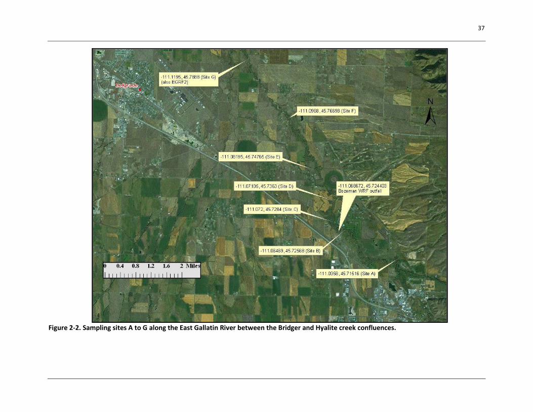
37
Figure 2-2. Sampling sites A to G along the East Gallatin River between the Bridger and Hyalite creek confluences.
38
Figure 2-3. Close-up of the three sampling sites around the city of Bozeman WRF discharge. Green dot is USGS gage 06048700.
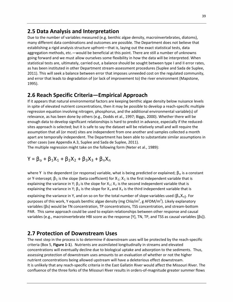
39
2.5 Data Analysis and Interpretation Due to the number of variables measured (e.g. benthic algae density, macroinvertebrates, diatoms), many different data combinations and outcomes are possible. The Department does not believe that establishing a rigid analysis structure upfront—that is, laying out the exact statistical tests, data aggregation methods, etc.—would be beneficial at this point. There are still a number of unknowns going forward and we must allow ourselves some flexibility in how the data will be interpreted. When statistical tests are, ultimately, carried out, a balance should be sought between type I and II error rates, as has been instituted in other Department stream-assessment procedures (Suplee and Sada de Suplee, 2011). This will seek a balance between error that imposes unneeded cost on the regulated community, and error that leads to degradation of (or lack of improvement to) the river environment (Mapstone, 1995).
2.6 Reach Specific Criteria—Empirical Approach If it appears that natural environmental factors are keeping benthic algae density below nuisance levels in spite of elevated nutrient concentrations, then it may be possible to develop a reach-specific multiple regression equation involving nitrogen, phosphorus, and the additional environmental variable(s) of relevance, as has been done by others (e.g., Dodds et al., 1997; Biggs, 2000). Whether there will be enough data to develop significant relationships is hard to predict in advance, especially if the reduced-sites approach is selected; but it is safe to say the dataset will be relatively small and will require the assumption that all (or most) sites are independent from one another and samples collected a month apart are temporally independent. The Department has been able to substantiate similar assumptions in other cases (see Appendix A.3, Suplee and Sada de Suplee, 2011). The multiple regression might take on the following form (Neter et al., 1989):
Y = βo + β1X1 + β2X2 + β3X3 + βnXn
where Y is the dependent (or response) variable, what is being predicted or explained; βo is a constant or Y-intercept; β1 is the slope (beta coefficient) for X1; X1 is the first independent variable that is explaining the variance in Y; β2 is the slope for X2; X2 is the second independent variable that is explaining the variance in Y; β3 is the slope for X3 and X3 is the third independent variable that is
explaining the variance in Y, and on so on for the total number of slope∙variables used (βnXn). For purposes of this work, Y equals benthic algae density (mg Chla/m2, g AFDM/m2). Likely explanatory variables (βs) would be TN concentration, TP concentrations, TSS concentration, and stream-bottom PAR. This same approach could be used to explain relationships between other response and causal variables (e.g., macroinvertebrate HBI score as the response [Y], TN, TP, and TSS as causal variables [βs]).
2.7 Protection of Downstream Uses The next step in the process is to determine if downstream uses will be protected by the reach-specific criteria (Box 5, Figure 1-1). Nutrients are assimilated longitudinally in streams and elevated concentrations will eventually decline due to biological uptake and adsorption to the sediments. Thus, assessing protection of downstream uses amounts to an evaluation of whether or not the higher nutrient concentrations being allowed upstream will have a deleterious effect downstream. It is unlikely that any reach-specific criteria in the East Gallatin River would affect the Missouri River. The confluence of the three forks of the Missouri River results in orders-of-magnitude greater summer flows

40
than the East Gallatin River. For example, mean August flow in the Missouri River ~24 miles downstream of the three forks is around 2,747 ft3/sec, whereas in the Gallatin River at Logan it is 490 ft3/sec, and near the mouth of the East Gallatin River it is about 250 ft3/sec (USGS, 2002; PBS&J, 2011). The most likely impacts from reach-specific nutrient criteria would be in the reach of the East Gallatin River downstream of the Hyalite Creek confluence. The nitrogen criterion recommended for the East Gallatin River between Hyalite Creek and the confluence with the West Gallatin River is 290 µg TN/L, lower than the 300 µg TN/L for the Middle Rockies (Suplee and Watson, 2012). Data suggest that the stream is nitrogen limited (since TP is naturally elevated) and is the reason why a lower TN criterion has been recommended there. A relaxation of the nitrogen criterion upstream of Hyalite Creek could very well lead to use impacts if the nitrogen limitation is, consequently, alleviated. Two approaches (which tie to Box 5 in Figure 1-1) can be taken to address downstream effects: An empirical approach. If the sites along the East Gallatin River downstream from Hyalite Creek (sites H, I, and J) show a general immunity to elevated nutrients (and the reach upstream of Hyalite Creek does as well) due to some natural factor like elevated turbidity, then reach specific criteria in the East Gallatin River could be extended all the way from the Bridger Creek confluence to the confluence with the West Gallatin River, or even beyond, to the confluence with the Missouri River. However if the reach of the East Gallatin River downstream of the Hyalite Creek confluence shows biological impacts/nuisance algae above targets, then reach specific criteria that may be appropriate for the East Gallatin River further upstream will not protect downstream uses, and should not be put in place. A mechanistic modeling approach using QUAL2K. This approach links to Section 3.0. The model would extend the full length of the East Gallatin River, between the Bridger Creek and West Gallatin River confluences to ascertain whether nutrients at a certain concentration, moving downstream from the point where Hyalite Creek confluences with the East Gallatin, would impact the beneficial uses further downstream. Beneficial uses addressed by the model include DO delta, pH delta, and benthic algae density. Please note that the mechanistic model requires additional types of sampling and sampling sites (tributaries, irrigation withdrawals and returns) than the empirical approach; see Section 3.0. The next section discusses approaches that can be used to develop a mechanistic model.
3.0 Developing Reach Specific Criteria via the Mechanistic Modeling Approach Objective: Collect enough data along the East Gallatin River between the Bridger Creek confluence and the West Gallatin River confluence during a low-flow condition to be able to calibrate and confirm a mechanistic QUAL2K model of the study reach. This objective still requires adequate biological characterization of the reach, as outlined in Sections 2.1 through 2.5. Many sites described in Section 2.0 overlap with model sites described below; this was done in order to optimize sampling. To assure the reach is long enough to be able to judge the validity of the rate coefficients used in the model, the longitudinal distance must be sufficient to observe during calibration the decline in soluble nutrients, conversions to organic from algal death and recycling, etc. It is the Department’s judgment that the East Gallatin River can be effectively modeled if the reach from above the Bozeman WRF to the West Gallatin River confluence (Figure 3-1) is considered, a distance of approximately 25 stream miles. Mechanistic models for criteria derivation require a robust set of field observations including streamflow and water-quality data, measurements from continuously deployed sondes (including, at a minimum, dissolved oxygen, pH, temperature, conductivity, and turbidity), and biogeochemical kinetic

41
observations (if possible). The Department has a detailed Quality Assurance Project Plan (Suplee et al., 2006) and a technical report (Flynn and Suplee, 2011) on the use of the QUAL2K model for developing reach-specific nutrient criteria; the reader is referred to those documents for greater detail. Selected sites are best sampled during one low-flow summer and fall (i.e., a year with flows near the seasonal 14Q5 of the East Gallatin River [McCarthy, 2005] or, alternatively, sequential low-flow summers during the peak of the growing period. Consecutive years with base flows that are below average is preferred but may not always be possible. If, during the initial biological and water-quality characterization (Sections 2.1 through 2.5), it is found that herbicides are high enough to suppress algal growth, the model will be severely compromised. Therefore, herbicide data are best collected and then assessed in advance of the decision to complete the mechanistic model detailed below.
3.1 Sites Requiring Water Quality Sonde Deployment For the QUAL2K model, six sites are recommended (Figure 3-1). Sondes could be deployed continuously, or for a week to ten days in middle to late August and then again for another week to ten days in middle to late September, during period of relatively stable flow (or in two sequential Augusts if each has lower-than-average baseflow). Water quality samples for key model drivers (nutrient concentrations—which include total nitrogen, nitrate+nitrite, ammonia, total phosphorus, and soluble reactive phosphorus; TSS and ISS; alkalinity; hardness; CBOD20; Total Organic Carbon [TOC]; and benthic and phytoplankton algae) need to be collected at the six sites, at least once in August and once in September (or in sequential low flow years). These data collections could potentially be synchronized with the data collection in Section 2.1.
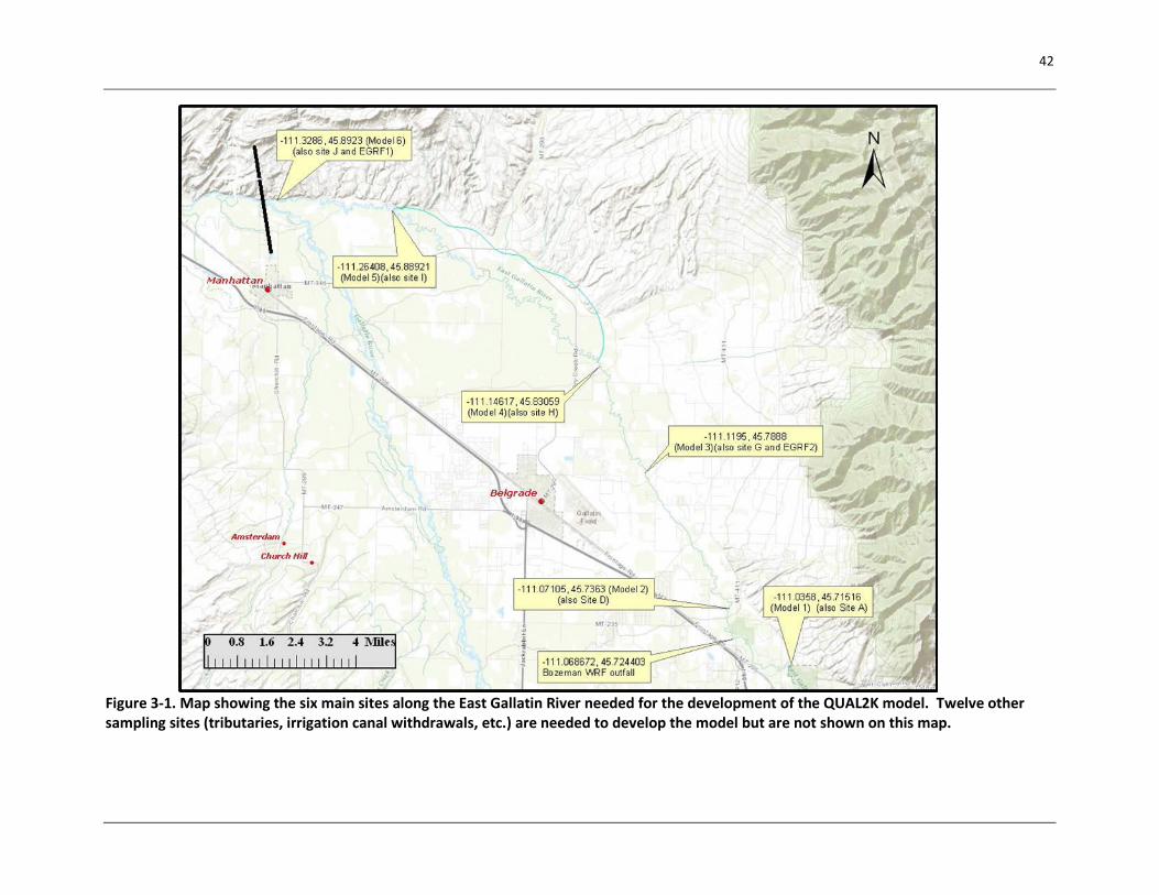
42
Figure 3-1. Map showing the six main sites along the East Gallatin River needed for the development of the QUAL2K model. Twelve other sampling sites (tributaries, irrigation canal withdrawals, etc.) are needed to develop the model but are not shown on this map.
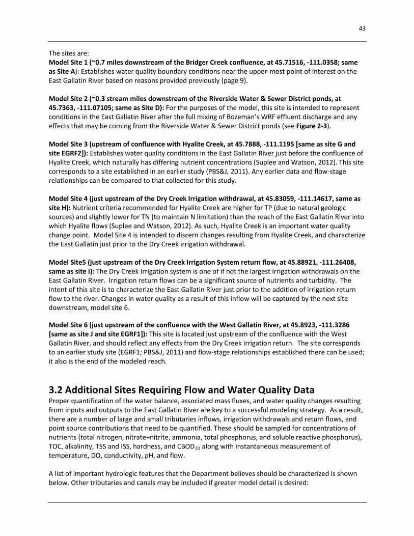
43
The sites are: Model Site 1 (~0.7 miles downstream of the Bridger Creek confluence, at 45.71516, -111.0358; same as Site A): Establishes water quality boundary conditions near the upper-most point of interest on the East Gallatin River based on reasons provided previously (page 9). Model Site 2 (~0.3 stream miles downstream of the Riverside Water & Sewer District ponds, at 45.7363, -111.07105; same as Site D): For the purposes of the model, this site is intended to represent conditions in the East Gallatin River after the full mixing of Bozeman’s WRF effluent discharge and any effects that may be coming from the Riverside Water & Sewer District ponds (see Figure 2-3). Model Site 3 (upstream of confluence with Hyalite Creek, at 45.7888, -111.1195 [same as site G and site EGRF2]): Establishes water quality conditions in the East Gallatin River just before the confluence of Hyalite Creek, which naturally has differing nutrient concentrations (Suplee and Watson, 2012). This site corresponds to a site established in an earlier study (PBS&J, 2011). Any earlier data and flow-stage relationships can be compared to that collected for this study. Model Site 4 (just upstream of the Dry Creek Irrigation withdrawal, at 45.83059, -111.14617, same as site H): Nutrient criteria recommended for Hyalite Creek are higher for TP (due to natural geologic sources) and slightly lower for TN (to maintain N limitation) than the reach of the East Gallatin River into which Hyalite flows (Suplee and Watson, 2012). As such, Hyalite Creek is an important water quality change point. Model Site 4 is intended to discern changes resulting from Hyalite Creek, and characterize the East Gallatin just prior to the Dry Creek irrigation withdrawal. Model Site5 (just upstream of the Dry Creek Irrigation System return flow, at 45.88921, -111.26408, same as site I): The Dry Creek Irrigation system is one of if not the largest irrigation withdrawals on the East Gallatin River. Irrigation return flows can be a significant source of nutrients and turbidity. The intent of this site is to characterize the East Gallatin River just prior to the addition of irrigation return flow to the river. Changes in water quality as a result of this inflow will be captured by the next site downstream, model site 6.
Model Site 6 (just upstream of the confluence with the West Gallatin River, at 45.8923, -111.3286 [same as site J and site EGRF1]): This site is located just upstream of the confluence with the West Gallatin River, and should reflect any effects from the Dry Creek irrigation return. The site corresponds to an earlier study site (EGRF1; PBS&J, 2011) and flow-stage relationships established there can be used; it also is the end of the modeled reach.
3.2 Additional Sites Requiring Flow and Water Quality Data Proper quantification of the water balance, associated mass fluxes, and water quality changes resulting from inputs and outputs to the East Gallatin River are key to a successful modeling strategy. As a result, there are a number of large and small tributaries inflows, irrigation withdrawals and return flows, and point source contributions that need to be quantified. These should be sampled for concentrations of nutrients (total nitrogen, nitrate+nitrite, ammonia, total phosphorus, and soluble reactive phosphorus), TOC, alkalinity, TSS and ISS, hardness, and CBOD20 along with instantaneous measurement of temperature, DO, conductivity, pH, and flow. A list of important hydrologic features that the Department believes should be characterized is shown below. Other tributaries and canals may be included if greater model detail is desired:
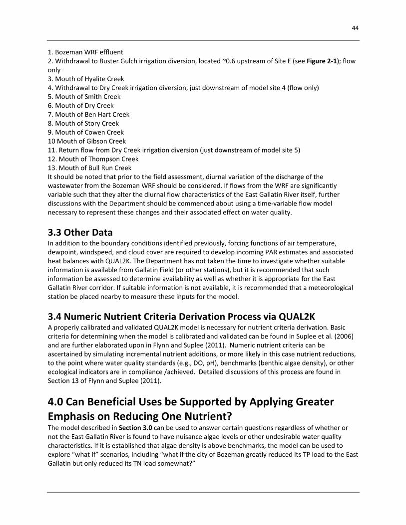
44
1. Bozeman WRF effluent 2. Withdrawal to Buster Gulch irrigation diversion, located ~0.6 upstream of Site E (see Figure 2-1); flow only 3. Mouth of Hyalite Creek 4. Withdrawal to Dry Creek irrigation diversion, just downstream of model site 4 (flow only) 5. Mouth of Smith Creek 6. Mouth of Dry Creek 7. Mouth of Ben Hart Creek 8. Mouth of Story Creek 9. Mouth of Cowen Creek 10 Mouth of Gibson Creek 11. Return flow from Dry Creek irrigation diversion (just downstream of model site 5) 12. Mouth of Thompson Creek 13. Mouth of Bull Run Creek It should be noted that prior to the field assessment, diurnal variation of the discharge of the wastewater from the Bozeman WRF should be considered. If flows from the WRF are significantly variable such that they alter the diurnal flow characteristics of the East Gallatin River itself, further discussions with the Department should be commenced about using a time-variable flow model necessary to represent these changes and their associated effect on water quality.
3.3 Other Data In addition to the boundary conditions identified previously, forcing functions of air temperature, dewpoint, windspeed, and cloud cover are required to develop incoming PAR estimates and associated heat balances with QUAL2K. The Department has not taken the time to investigate whether suitable information is available from Gallatin Field (or other stations), but it is recommended that such information be assessed to determine availability as well as whether it is appropriate for the East Gallatin River corridor. If suitable information is not available, it is recommended that a meteorological station be placed nearby to measure these inputs for the model.
3.4 Numeric Nutrient Criteria Derivation Process via QUAL2K A properly calibrated and validated QUAL2K model is necessary for nutrient criteria derivation. Basic criteria for determining when the model is calibrated and validated can be found in Suplee et al. (2006) and are further elaborated upon in Flynn and Suplee (2011). Numeric nutrient criteria can be ascertained by simulating incremental nutrient additions, or more likely in this case nutrient reductions, to the point where water quality standards (e.g., DO, pH), benchmarks (benthic algae density), or other ecological indicators are in compliance /achieved. Detailed discussions of this process are found in Section 13 of Flynn and Suplee (2011).
4.0 Can Beneficial Uses be Supported by Applying Greater Emphasis on Reducing One Nutrient? The model described in Section 3.0 can be used to answer certain questions regardless of whether or not the East Gallatin River is found to have nuisance algae levels or other undesirable water quality characteristics. If it is established that algae density is above benchmarks, the model can be used to explore “what if” scenarios, including “what if the city of Bozeman greatly reduced its TP load to the East Gallatin but only reduced its TN load somewhat?”
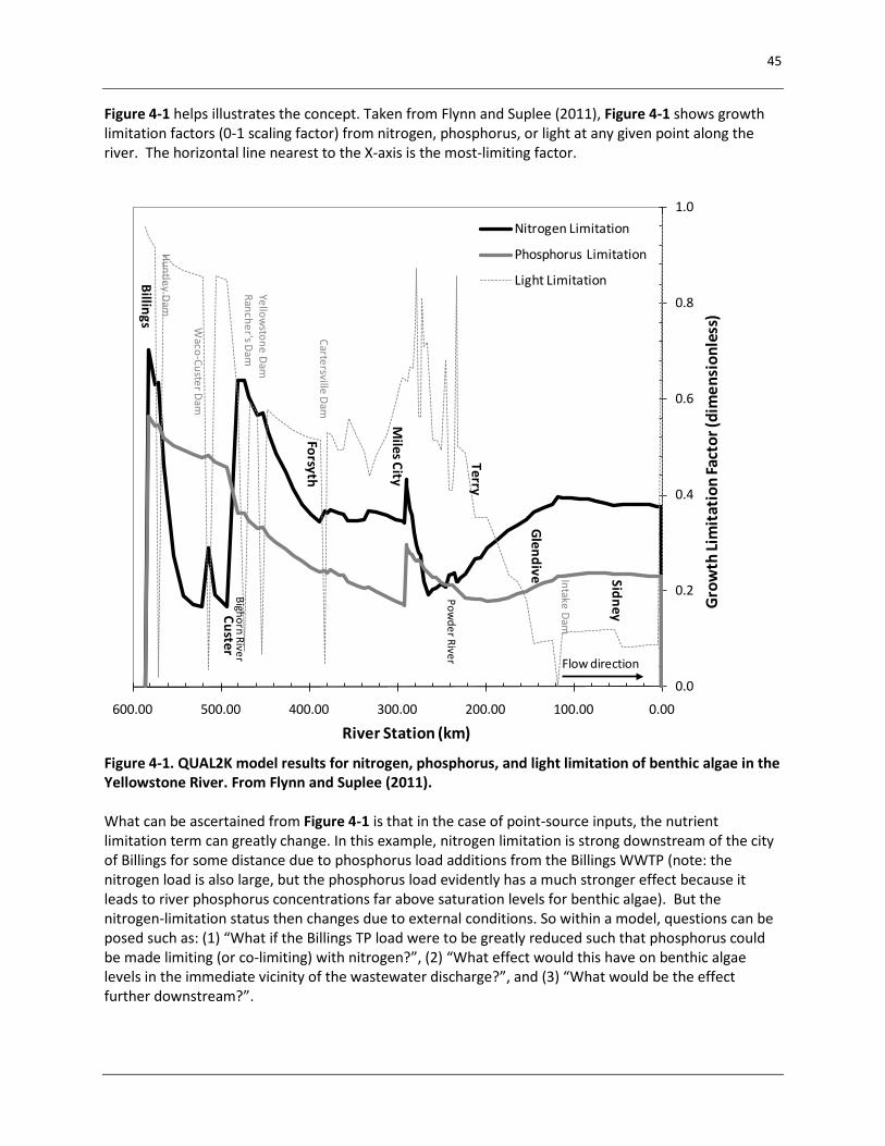
45
Figure 4-1 helps illustrates the concept. Taken from Flynn and Suplee (2011), Figure 4-1 shows growth limitation factors (0-1 scaling factor) from nitrogen, phosphorus, or light at any given point along the river. The horizontal line nearest to the X-axis is the most-limiting factor.
Figure 4-1. QUAL2K model results for nitrogen, phosphorus, and light limitation of benthic algae in the Yellowstone River. From Flynn and Suplee (2011). What can be ascertained from Figure 4-1 is that in the case of point-source inputs, the nutrient limitation term can greatly change. In this example, nitrogen limitation is strong downstream of the city of Billings for some distance due to phosphorus load additions from the Billings WWTP (note: the nitrogen load is also large, but the phosphorus load evidently has a much stronger effect because it leads to river phosphorus concentrations far above saturation levels for benthic algae). But the nitrogen-limitation status then changes due to external conditions. So within a model, questions can be posed such as: (1) “What if the Billings TP load were to be greatly reduced such that phosphorus could be made limiting (or co-limiting) with nitrogen?”, (2) “What effect would this have on benthic algae levels in the immediate vicinity of the wastewater discharge?”, and (3) “What would be the effect further downstream?”.
0.0
0.2
0.4
0.6
0.8
1.0
0.00100.00200.00300.00400.00500.00600.00Gr
owth
Lim
itatio
n Fa
ctor
(dim
ensi
onle
ss)
River Station (km)
Nitrogen Limitation
Phosphorus Limitation
Light Limitation
Miles City
Terry
Glendive
Forsyth
Billings
Sidney
Huntley Dam
Cartersville Dam
Intake Dam
Waco-Custer Dam
Yellowstone Dam
Rancher's DamBighorn River
Custer
Powder River Flow direction
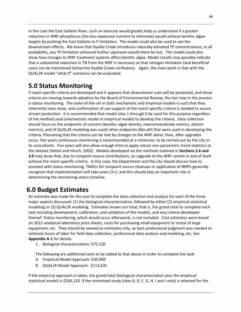
46
In the case the East Gallatin River, such an exercise would greatly help us understand if a greater reduction in WRF phosphorus (the less expensive nutrient to eliminate) would achieve benthic algae targets by pushing the East Gallatin to P limitation. The model could also be used to see the downstream effects. We know that Hyalite Creek introduces naturally-elevated TP concentrations; in all probability, any TP limitation achieved further upstream would there be lost. The model could also show how changes to WRF treatment systems affect benthic algae. Model results may possibly indicate that a substantial reduction in TN from the WRF is necessary so that nitrogen limitation (and beneficial uses) can be maintained below the Hyalite Creek confluence. Again, the main point is that with the QUAL2K model “what if” scenarios can be evaluated.
5.0 Status Monitoring If reach specific criteria are developed and it appears that downstream uses will be protected, and those criteria are moving towards adoption by the Board of Environmental Review, the last step in the process is status monitoring. The state-of-the-art in both mechanistic and empirical models is such that they inherently have noise, and confirmation of use-support of the reach-specific criteria is needed to assure stream protection. It is recommended that model sites 1 through 6 be used for this purpose regardless of the method used (mechanistic model or empirical model) to develop the criteria. Data collection should focus on the endpoints of concern (benthic algae density, macroinverebrate metrics, diatom metrics), and (if QUAL2K modeling was used) other endpoints (like pH) that were used in developing the criteria. Presuming that the criteria can be met by changes to the WRF alone, then, after upgrades occur, five years continuous monitoring is recommended at a minimum, to be carried out by the city or its consultants. Five years will also allow enough time to apply robust non-parametric trend statistics to the dataset (Helsel and Hirsch, 2002). Models developed via the methods outlined in Sections 2.6 and 3.0 may show that, due to nonpoint source contributions, an upgrade to the WRF cannot in and of itself achieve the reach-specific criteria. In this case, the Department and the city should discuss how to proceed with status monitoring. TMDLs for nonpoint source cleanups or application of BMPs generally recognize that implementation will take years (5+), and this should play an important role in determining the monitoring status timeline.
6.0 Budget Estimates An estimate was made for the cost to complete the data collection and analysis for each of the three major aspects discussed: (1) the biological characterization, followed by either (2) empirical statistical modeling or (3) QUAL2K modeling. Estimates shown are total, that is, the grand total to complete each task including development, calibration, and validation of the models, and any criteria developed thereof. Status monitoring, which would occur afterwards, is not included. Cost estimates were based on 2012 analytical laboratory price sheets, costs for purchasing small equipment or rental of large equipment, etc. They should be viewed as estimates only, as best professional judgment was needed to estimate hours of labor for field data collection, professional data analysis and modeling, etc. See Appendix A-1 for details.
1. Biological characterization: $75,220
The following are additional costs to be added to that above in order to complete the task: A. Empirical Model Approach: $30,900 B. QUAL2K Model Approach: $113,635
If the empirical approach is taken, the grand total (biological characterization plus the empirical statistical model) is $106,120. If the minimized study (sites B, D, F, G, H, I and J only) is selected for the
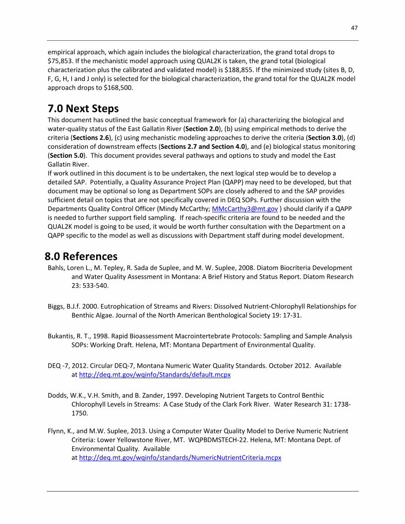
47
empirical approach, which again includes the biological characterization, the grand total drops to $75,853. If the mechanistic model approach using QUAL2K is taken, the grand total (biological characterization plus the calibrated and validated model) is $188,855. If the minimized study (sites B, D, F, G, H, I and J only) is selected for the biological characterization, the grand total for the QUAL2K model approach drops to $168,500.
7.0 Next Steps This document has outlined the basic conceptual framework for (a) characterizing the biological and water-quality status of the East Gallatin River (Section 2.0), (b) using empirical methods to derive the criteria (Sections 2.6), (c) using mechanistic modeling approaches to derive the criteria (Section 3.0), (d) consideration of downstream effects (Sections 2.7 and Section 4.0), and (e) biological status monitoring (Section 5.0). This document provides several pathways and options to study and model the East Gallatin River. If work outlined in this document is to be undertaken, the next logical step would be to develop a detailed SAP. Potentially, a Quality Assurance Project Plan (QAPP) may need to be developed, but that document may be optional so long as Department SOPs are closely adhered to and the SAP provides sufficient detail on topics that are not specifically covered in DEQ SOPs. Further discussion with the Departments Quality Control Officer (Mindy McCarthy; [email protected] ) should clarify if a QAPP is needed to further support field sampling. If reach-specific criteria are found to be needed and the QUAL2K model is going to be used, it would be worth further consultation with the Department on a QAPP specific to the model as well as discussions with Department staff during model development.
8.0 References Bahls, Loren L., M. Tepley, R. Sada de Suplee, and M. W. Suplee, 2008. Diatom Biocriteria Development
and Water Quality Assessment in Montana: A Brief History and Status Report. Diatom Research 23: 533-540.
Biggs, B.J.f. 2000. Eutrophication of Streams and Rivers: Dissolved Nutrient-Chlorophyll Relationships for Benthic Algae. Journal of the North American Benthological Society 19: 17-31.
Bukantis, R. T., 1998. Rapid Bioassessment Macrointertebrate Protocols: Sampling and Sample Analysis SOPs: Working Draft. Helena, MT: Montana Department of Environmental Quality.
DEQ -7, 2012. Circular DEQ-7, Montana Numeric Water Quality Standards. October 2012. Available at http://deq.mt.gov/wqinfo/Standards/default.mcpx
Dodds, W.K., V.H. Smith, and B. Zander, 1997. Developing Nutrient Targets to Control Benthic Chlorophyll Levels in Streams: A Case Study of the Clark Fork River. Water Research 31: 1738-1750.
Flynn, K., and M.W. Suplee, 2013. Using a Computer Water Quality Model to Derive Numeric Nutrient
Criteria: Lower Yellowstone River, MT. WQPBDMSTECH-22. Helena, MT: Montana Dept. of Environmental Quality. Available at http://deq.mt.gov/wqinfo/standards/NumericNutrientCriteria.mcpx
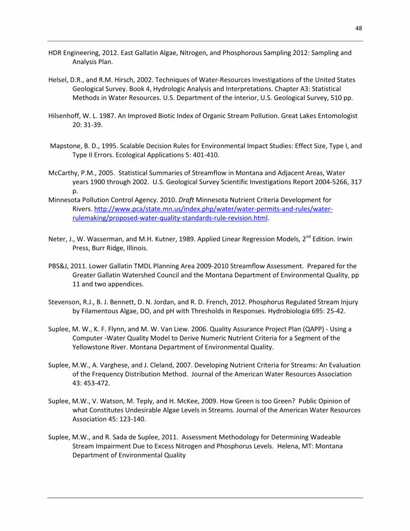
48
HDR Engineering, 2012. East Gallatin Algae, Nitrogen, and Phosphorous Sampling 2012: Sampling and Analysis Plan.
Helsel, D.R., and R.M. Hirsch, 2002. Techniques of Water-Resources Investigations of the United States
Geological Survey. Book 4, Hydrologic Analysis and Interpretations. Chapter A3: Statistical Methods in Water Resources. U.S. Department of the Interior, U.S. Geological Survey, 510 pp.
Hilsenhoff, W. L. 1987. An Improved Biotic Index of Organic Stream Pollution. Great Lakes Entomologist
20: 31-39.
Mapstone, B. D., 1995. Scalable Decision Rules for Environmental Impact Studies: Effect Size, Type I, and Type II Errors. Ecological Applications 5: 401-410.
McCarthy, P.M., 2005. Statistical Summaries of Streamflow in Montana and Adjacent Areas, Water
years 1900 through 2002. U.S. Geological Survey Scientific Investigations Report 2004-5266, 317 p.
Minnesota Pollution Control Agency. 2010. Draft Minnesota Nutrient Criteria Development for Rivers. http://www.pca/state.mn.us/index.php/water/water-permits-and-rules/water-rulemaking/proposed-water-quality-standards-rule-revision.html.
Neter, J., W. Wasserman, and M.H. Kutner, 1989. Applied Linear Regression Models, 2nd Edition. Irwin Press, Burr Ridge, Illinois.
PBS&J, 2011. Lower Gallatin TMDL Planning Area 2009-2010 Streamflow Assessment. Prepared for the
Greater Gallatin Watershed Council and the Montana Department of Environmental Quality, pp 11 and two appendices.
Stevenson, R.J., B. J. Bennett, D. N. Jordan, and R. D. French, 2012. Phosphorus Regulated Stream Injury
by Filamentous Algae, DO, and pH with Thresholds in Responses. Hydrobiologia 695: 25-42. Suplee, M. W., K. F. Flynn, and M. W. Van Liew. 2006. Quality Assurance Project Plan (QAPP) - Using a
Computer -Water Quality Model to Derive Numeric Nutrient Criteria for a Segment of the Yellowstone River. Montana Department of Environmental Quality.
Suplee, M.W., A. Varghese, and J. Cleland, 2007. Developing Nutrient Criteria for Streams: An Evaluation
of the Frequency Distribution Method. Journal of the American Water Resources Association 43: 453-472.
Suplee, M.W., V. Watson, M. Teply, and H. McKee, 2009. How Green is too Green? Public Opinion of
what Constitutes Undesirable Algae Levels in Streams. Journal of the American Water Resources Association 45: 123-140.
Suplee, M.W., and R. Sada de Suplee, 2011. Assessment Methodology for Determining Wadeable
Stream Impairment Due to Excess Nitrogen and Phosphorus Levels. Helena, MT: Montana Department of Environmental Quality

49
Suplee, M.W., V. Watson, W.K. Dodds, and C. Shirley, 2012. Response of Algal Biomass to Large Scale Nutrient Controls on the Clark Fork River, Montana, United States. Journal of the American Water Resources Association 48: 1008-1021.
Suplee, M.W. and V. Watson, 2013. Scientific and Technical Basis of the Numeric Nutrient Criteria for
Montana’s Wadeable Streams and Rivers: Update 1. Final Draft. Helena, MT: Montana Dept. of Environmental Quality. Available at http://deq.mt.gov/wqinfo/standards/NumericNutrientCriteria.mcpx
Teply, M. 2010a. Interpretation of Periphyton Samples From Montana Streams. Lacey, WA: Cramer Fish
Sciences.
Teply, Mark. 2010b. Diatom Biocriteria for Montana Streams. Lacey, WA: Cramer Fish Sciences.
Tetra Tech (Tetra Tech, Inc.), 2010. Analysis of Montana Nutrient and Biological Data for the Nutrient Scientific Technical Exchange Partnership Support (N-STEPS).Prepared for the U.S. Environmental Protection Agency, Office of Science and Technology.
USGS (U.S. Geological Survey), 1999. Effluent Mixing Characteristics below Four Wastewater-Treatment
Facilities in Southwestern Montana, 1997. Water Resources Investigations Report 99-4026. USGS (U.S. Geological Survey), 2004. Water Resources Data Montana Water Year 2002. Water Data
Report MT-02-1. USGS (U.S. Geological Survey), 2004. Water Quality Assessment of the Yellowstone River Basin, Montana
and Wyoming—Water Quality of Fixed Sites, 1999-2001. Scientific Investigations Report 2004-5113.
WQPBWQM-0090, 2012. Montana Department of Environmental Quality, Sample Collection, Sorting,
Taxonomic Identification, and Analysis of Benthic Macroinvertebrate Communities Standard Operating Procedure. March 15, 2012. Available at http://deq.mt.gov/wqinfo/qaprogram/sops.mcpx
WQPBWQM-020, 2012. Montana Department of Environmental Quality, Water Quality Planning Bureau
Field Procedures Manual for Water Quality Assessment Monitoring. February 2012. Available at http://deq.mt.gov/wqinfo/qaprogram/sops.mcpx
WQPBWQM-010, 2011. Montana Department of Environmental Quality, Periphyton Standard Operating
Procedure. February 18, 2011. Available at http://deq.mt.gov/wqinfo/qaprogram/sops.mcpx WQPBWQM-011, 2011. Montana Department of Environmental Quality, Sample Collection and
Laboratory Analysis of Chlorophyll-a Standard Operating Procedure. December 21, 2011. Available at http://deq.mt.gov/wqinfo/qaprogram/sops.mcpx

Nutrient Standards Implementation Guidance
Appendix A-1
1. Biological Characterization (2-year study, up to three months per summer). This work is undertaken regardless of preferred modeling approach. Benthic Algae (Chla ) Benthic Algae (AFDM) Macroinvertebrates Diatoms WQ (nutrients, TSS)* Herbicides**
SITE Frequency Cost/sample Frequency Cost/sample Frequency Cost/sample Frequency Cost/sample Frequency Cost/sample Frequency Cost/sample
A 6 $1,170 6 $300 4 $980 2 $500 6 $960.00 5 $750
B 6 $1,170 6 $300 4 $980 2 $500 6 $960.00 5 $750
C 6 $1,170 6 $300 4 $980 2 $500 6 $960.00 5 $750
D 6 $1,170 6 $300 4 $980 2 $500 6 $960.00 5 $750
E 6 $1,170 6 $300 4 $980 2 $500 6 $960.00 5 $750
F 6 $1,170 6 $300 4 $980 2 $500 6 $960.00 5 $750
G 6 $1,170 6 $300 4 $980 2 $500 6 $960.00 5 $750
H 6 $1,170 6 $300 2 $490 1 $250 6 $960.00 5 $750
I 6 $1,170 6 $300 2 $490 1 $250 6 $960.00 5 $750
J 6 $1,170 6 $300 2 $490 1 $250 6 $960.00 5 $750Totals: $11,700 $3,000 $8,330 $4,250 $9,600 $7,500
Subtotals, analytical costs:
$44,380
YSI 6600 Sonde Rental:$2,240
Assume 2 sondes, deployed for 1 week each summer for two summers ($560 X 2 X 2). * TSS $20.00Purchase YSI 85 $1,350 For instantaneous DO, temperature, and conductivity. Separate low-cost pH meter can be purchased. TN $40.00Labor in field: $14,250 Assume a field team of 2 people, 10 sites, 3 hrs/site, average of 4.75 trips per site (for both years), assume $50/hr. TP $30.00Data analysi:s $10,000 Assume 1 person, contracted, professional environmental consulting firm SRP $30.00
Misc. supplies: $3,000 macroinvertebrate nets, filters, filter apperatus, vehicle gasoline, etc. nitrate + nitrite $25.00
GRAND TOTAL, Biological
Characterization:$75,220 total ammonia $15.00
Analytical (min sites) Field labor (min sites) $160.00
$28,300 $9,975 GRAND TOTAL, min. sites (B, C, F, G, H, I, J): $54,865
**N, P, and S containing pesticides (Method E507 modified).
5/15/12 Draft 1

Nutrient Standards Implementation Guidance
2. Statistical Empirical Model (One additional year of data in additional to the biological characterization). Benthic Algae (Chla ) Benthic Algae (AFDM) Macroinvertebrates Diatoms WQ (nutrients, TSS)* Herbicides
SITE Frequency Cost/sample Frequency Cost/sample Frequency Cost/sample Frequency Cost/sample Frequency Cost/sample Frequency Cost/sample
A 3 $585 3 $150 2 $490 1 $250 3 $480.00 2 $300
B 3 $585 3 $150 2 $490 1 $250 3 $480.00 2 $300
C 3 $585 3 $150 2 $490 1 $250 3 $480.00 2 $300
D 3 $585 3 $150 2 $490 1 $250 3 $480.00 2 $300
E 3 $585 3 $150 2 $490 1 $250 3 $480.00 2 $300
F 3 $585 3 $150 2 $490 1 $250 3 $480.00 2 $300
G 3 $585 3 $150 2 $490 1 $250 3 $480.00 2 $300
H 3 $585 3 $150 2 $490 1 $250 3 $480.00 2 $300
I 3 $585 3 $150 2 $490 1 $250 3 $480.00 2 $300
J 3 $585 3 $150 2 $490 1 $250 3 $480.00 2 $300Totals: $5,850 $1,500 $4,900 $2,500 $4,800 $3,000
Subtotals, analytical costs:
$22,550
YSI 6600 Sonde Rental:$560 Assume 1sondes, deployed for 1 week for 1 summers ($560 X 1 X 1).
Labor in field: $6,990 Assume a field team of 2 people, 10 sites, 3 hrs/site, average of 2.333 trips per site, assume $50/hr.Data analysi:s $15,000 Assume 1 person, contracted, professional environmental consulting firm. This would be final report and emperical model development
Misc. supplies: $800 macroinvertebrate nets, filters, filter apperatus, vehicle gasoline, etc. Year 3 Total: $30,900
Emperical Model, TOTAL ‡ :
$106,120Analytical (min sites) Field labor (min sites)
$14,735 $4,893 Year 3 Total, min. sites (B, C, F, G H, I, J): $20,988
Emperical Model, TOTAL, min sites (B, C, F, G, H, I, J) ‡ : $75,853
5/15/12 Draft 2
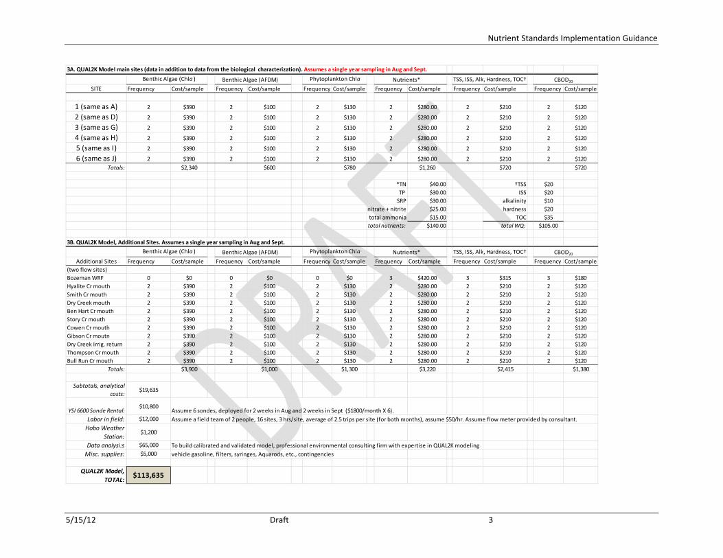
Nutrient Standards Implementation Guidance
3A. QUAL2K Model main sites (data in addition to data from the biological characterization). Assumes a single year sampling in Aug and Sept. Benthic Algae (Chla ) Benthic Algae (AFDM) Phytoplankton Chla Nutrients* CBOD20
SITE Frequency Cost/sample Frequency Cost/sample Frequency Cost/sample Frequency Cost/sample Frequency Cost/sample Frequency Cost/sample
1 (same as A) 2 $390 2 $100 2 $130 2 $280.00 2 $210 2 $120
2 (same as D) 2 $390 2 $100 2 $130 2 $280.00 2 $210 2 $120
3 (same as G) 2 $390 2 $100 2 $130 2 $280.00 2 $210 2 $120
4 (same as H) 2 $390 2 $100 2 $130 2 $280.00 2 $210 2 $120
5 (same as I) 2 $390 2 $100 2 $130 2 $280.00 2 $210 2 $120
6 (same as J) 2 $390 2 $100 2 $130 2 $280.00 2 $210 2 $120Totals: $2,340 $600 $780 $1,260 $720 $720
*TN $40.00 †TSS $20TP $30.00 ISS $20
SRP $30.00 alkalinity $10nitrate + nitrite $25.00 hardness $20total ammonia $15.00 TOC $35total nutrients: $140.00 total WQ: $105.00
3B. QUAL2K Model, Additional Sites. Assumes a single year sampling in Aug and Sept. Benthic Algae (Chla ) Benthic Algae (AFDM) Phytoplankton Chla Nutrients* CBOD20
Additional Sites Frequency Cost/sample Frequency Cost/sample Frequency Cost/sample Frequency Cost/sample Frequency Cost/sample Frequency Cost/sample(two flow sites)Bozeman WRF 0 $0 0 $0 0 $0 3 $420.00 3 $315 3 $180Hyalite Cr mouth 2 $390 2 $100 2 $130 2 $280.00 2 $210 2 $120Smith Cr mouth 2 $390 2 $100 2 $130 2 $280.00 2 $210 2 $120Dry Creek mouth 2 $390 2 $100 2 $130 2 $280.00 2 $210 2 $120Ben Hart Cr mouth 2 $390 2 $100 2 $130 2 $280.00 2 $210 2 $120Story Cr mouth 2 $390 2 $100 2 $130 2 $280.00 2 $210 2 $120Cowen Cr mouth 2 $390 2 $100 2 $130 2 $280.00 2 $210 2 $120Gibson Cr moutn 2 $390 2 $100 2 $130 2 $280.00 2 $210 2 $120Dry Creek Irrig. return 2 $390 2 $100 2 $130 2 $280.00 2 $210 2 $120Thompson Cr mouth 2 $390 2 $100 2 $130 2 $280.00 2 $210 2 $120Bull Run Cr mouth 2 $390 2 $100 2 $130 2 $280.00 2 $210 2 $120
Totals: $3,900 $1,000 $1,300 $3,220 $2,415 $1,380
Subtotals, analytical costs:
$19,635
YSI 6600 Sonde Rental:$10,800
Assume 6 sondes, deployed for 2 weeks in Aug and 2 weeks in Sept ($1800/month X 6).Labor in field: $12,000 Assume a field team of 2 people, 16 sites, 3 hrs/site, average of 2.5 trips per site (for both months), assume $50/hr. Assume flow meter provided by consultant.
Hobo Weather Station:
$1,200
Data analysi:s $65,000 To build calibrated and validated model, professional environmental consulting firm with expertise in QUAL2K modelingMisc. supplies: $5,000 vehicle gasoline, filters, syringes, Aquarods, etc., contingencies
QUAL2K Model, TOTAL: $113,635
TSS, ISS, Alk, Hardness, TOC†
TSS, ISS, Alk, Hardness, TOC†
5/15/12 Draft 3

Nutrient Standards Implementation Guidance
5/15/12 Draft 4
Related Documents