Dr. Nestler - Math 11 - Some Definitions and Theorems from Calculus 1 and 2 Definition continuous . A function is at a number if . 0 + 0 ÐBÑ œ 0 Ð+Ñ lim BÄ+ Extreme Value Theorem . A continuous function on a closed interval has an absolute maximum value and an absolute minimum value on that interval. Definition derivative . The of a function at a number is the number 0 + if this limit exists. 0 Ð+Ñ œ œ w 2Ä! 0 Ð+2Ñ0 Ð+Ñ 0 ÐBÑ0 Ð+Ñ 2 B+ BÄ+ lim lim Theorem & Definition . Suppose is continuous on . Divide into subintervals 0 Ò+ß ,Ó Ò+ß ,Ó 8 of equal length , and choose a number in for each . ÒB ßBÓ B A ÒB ßBÓ 3 œ "ß á ß 8 3" 3 3 3" 3 ? Then exists, and this number is called the lim 8Ä∞ 3œ" 8 3 0 ÐA Ñ B ? definite integral of from 0 + to ,, and is denoted by . + , 0ÐBÑ.B Fundamental Theorem of Calculus, Part I . If is continuous on , then 0 Ò+ß ,Ó J ÐBÑ œ 0Ð>Ñ.> + B is an antiderivative of , meaning for all in . 0 J ÐBÑ œ 0ÐBÑ B Ò+ß ,Ó w Fundamental Theorem of Calculus, Part II. If is any antiderivative of on , then J 0 Ò+ß ,Ó . + , 0 ÐBÑ .B œ J Ð,Ñ J Ð+Ñ Mean Value Theorem for Differentiable Functions . If is continuous on and differentiable 0 Ò+ß ,Ó on , then there exists at least one in such that . That is, Ð+ß ,Ñ - Ð+ß ,Ñ œ 0 Ð-Ñ 0Ð,Ñ0Ð+Ñ ,+ w 0 Ð,Ñ 0 Ð+Ñ œ 0 Ð-ÑÐ, +ÑÞ w Inverse Function Theorem . If is differentiable with inverse , and , C œ 0ÐBÑ 0 0 Ð0 Ð+ÑÑ Á ! " w " then is differentiable at , and 0 + " .0 .B Bœ+ " " œ .0 .B Bœ0 Ð+Ñ " Shorthand: .B " .C œ .C .B

Welcome message from author
This document is posted to help you gain knowledge. Please leave a comment to let me know what you think about it! Share it to your friends and learn new things together.
Transcript

Dr. Nestler - Math 11 - Some Definitions and Theorems from Calculus 1 and 2
Definition continuous. A function is at a number if .0 + 0ÐBÑ œ 0Ð+ÑlimBÄ+
Extreme Value Theorem. A continuous function on a closed interval has an absolute maximum
value and an absolute minimum value on that interval.
Definition derivative. The of a function at a number is the number0 +
if this limit exists.0 Ð+Ñ œ œw
2Ä!
0Ð+2Ñ0Ð+Ñ 0ÐBÑ0Ð+Ñ2 B+BÄ+
lim lim
Theorem & Definition. Suppose is continuous on . Divide into subintervals0 Ò+ß ,Ó Ò+ß ,Ó 8
of equal length , and choose a number in for each .ÒB ß B Ó B A ÒB ß B Ó 3 œ "ßá ß 83" 3 3 3" 3?
Then exists, and this number is called the lim8Ä∞ 3œ"
8
30ÐA Ñ B? definite integral of from 0 +
to ,, and is denoted by .+,0ÐBÑ .B
Fundamental Theorem of Calculus, Part I. If is continuous on , then 0 Ò+ß ,Ó J ÐBÑ œ 0Ð>Ñ .>+B
is an antiderivative of , meaning for all in .0 J ÐBÑ œ 0ÐBÑ B Ò+ß ,Ów
Fundamental Theorem of Calculus, Part II. If is any antiderivative of on , thenJ 0 Ò+ß ,Ó
.+,0ÐBÑ .B œ JÐ,Ñ JÐ+Ñ
Mean Value Theorem for Differentiable Functions. If is continuous on and differentiable0 Ò+ß ,Ó
on , then there exists at least one in such that . That is,Ð+ß ,Ñ - Ð+ß ,Ñ œ 0 Ð-Ñ0Ð,Ñ0Ð+Ñ,+
w
0Ð,Ñ 0Ð+Ñ œ 0 Ð-ÑÐ, +ÑÞw
Inverse Function Theorem. If is differentiable with inverse , and ,C œ 0ÐBÑ 0 0 Ð0 Ð+ÑÑ Á !" w "
then is differentiable at , and0 +"
.0.B Bœ+
"" œ .0.B Bœ0 Ð+Ñ"
Shorthand: .B ".C œ .C
.B

Dr. Nestler - Math 11 - Essential Trigonometric and Hyperbolic Function Identities
Fundamental trigonometric identities:
csc sec tan cot B œ B œ B œ B œ œ" " B B "B B B B Bsin cos cos sin tan
sin cos
sin cos tan sec cot csc# # # # # #B B œ " B " œ B " B œ B
sin sin cos cosÐBÑ œ B ÐBÑ œ ÐBÑ Double-angle identities:
sin sin cos cos cos sin sin cos#B œ # B B #B œ B B œ " # B œ # B "# # # #
Half-angle identities:
sin cos# #" #B " BB œ B œcos cos 22 2
Trigonometric derivatives:
. . ..B .B .B
#Ð BÑ œ B Ð BÑ œ B Ð BÑ œ Bsin cos cos sin tan sec
. . ..B .B .B
#Ð BÑ œ B B Ð BÑ œ B B Ð BÑ œ Bsec sec tan csc csc tan cot csc
Inverse trigonometric derivatives:
. " . " . ".B .B "B .B
" " "
"B B B "Ð BÑ œ lBl " Ð BÑ œ Ð BÑ œ lBl "sin ( ) tan sec ( ) # ##
Hyperbolic definitions and fundamental identities:
cosh sinh tanh B œ B œ B œ/ / / / B# # B
B B B B sinh cosh
sech csch coth B œ B œ B œ œ" " B "B B B Bcosh sinh sinh tanh
cosh
cosh sinh sinh sinh cosh cosh# #B B œ " ÐBÑ œ B ÐBÑ œ ÐBÑ Hyperbolic derivatives:
. . ..B .B .B
#Ð BÑ œ B B œ B Ð BÑ œ Bsinh cosh cosh sinh tanh sech . . ..B .B .B
#Ð BÑ œ B B B œ B B B œ Bsech sech tanh csch csch coth coth csch

Dr. Nestler - Math 11 - 12.6 - Surfaces
A is a two-dimensional graph of an equation in , , .surface B C D
1. sphere:
2. plane:
3. : a surface consisting of all lines ( ) that are parallel to a fixed line and passingcylinder rulings through a fixed plane curve ( )directrix
Example: C D œ "'# #
is arbitrary: cross-sections perpendicular to the -axis are circles of radius 4.B B
. The graph of an eqn. in 2 of the 3 variablesThm , , is a cylinder whose rulings are parallel toB C D the axis of the missing variable.
Example: Cross-sections perpendicular to the -axis are parabolas.D œ B C#
4. Except for degenerate cases, a is a graph of a quadratic equation in 3 variablesquadric surface
EB FC GD HBC ICD JBD KB LC MD N œ !# # #
which by translation and rotation can be put into standard form
EB FC GD N œ !# # #
or .EB FC MD œ !# #
Traces in planes parallel to the coordinate planes are conic sections.
Some degenerate examples: , , B œ ! B œ + B C D œ !# # # # # #

Example: B D+ , -
C# #
# # #
#
œ "
: trace in -plane is ellipseB œ ! CD
: trace in -plane is ellipseC œ ! BD
: trace in -plane is ellipseD œ ! BC
The surface is called an ellipsoid.
Example: B D+ , -
C# #
# # #
#
œ "
: trace in -plane is ellipseD œ ! BC
: trace in -plane is hyperbolaB œ ! CD
: trace in -plane is hyperbolaC œ ! BD
Let : D œ 5 B 5+ , -
C# #
# # #
#
œ "
B
+ " , "
C#
# #5 5# #
- -# #
#
œ "
Cross-sections parallel to the -plane are ellipses. As , ellipses get larger.BC l5l Ä ∞
The surface is called a . The -axis,hyperboloid of one sheet elliptic hyperboloid or an D corresponding to the minus sign in the equation, is the axis of the hyperboloid.
Example: This is a hyperboloid of one sheet with the -axis as its axis. B D+ , -
C# #
# # #
#
œ " C
Similarly, the graph of is a hyperboloid of one sheet with the œ "B D+ , -
C# #
# # #
#
-axis as its axis.B

Example: œ "B D+ , -
C# #
# # #
#
: no trace in -planeD œ ! BC
: trace in -plane is hyperbolaB œ ! CD
: trace in -plane is hyperbolaC œ ! BD
The surface is called a .hyperboloid of two sheets
The -axis, corresponding to the plus sign in the equation, is the axis of the hyperboloid.D
Example: B D+ , -
C# #
# # #
#
œ "
The axis of this hyperboloid of two sheets is the -axis, and there is no trace in theB -plane. (Try letting .)CD B œ !
Example: B D+ , -
C# #
# # #
#
œ !
: Cross-sections parallel to the -plane are ellipses.D œ 5 BC
D œ „ - B+ ,
C#
# #
#
The surface is a ( ) with the -axis as its axis.double-napped elliptic cone D
Examples: The graph of is a cone with the -axis as its axis. B D+ , -
C# #
# # #
#
œ ! C
The graph of is a cone with the -axis as its axis. BB D+ , -
C# #
# # #
#
œ !

Example: B+ ,C#
# #
#
D œ !
: trace is parabola B œ ! D œ C,
#
# opening up
: trace is parabola C œ ! D œ B+
#
# opening up
: Cross-sections parallel to -plane are ellipses.D œ 5 ! BC
The surface is called an . The -axis, corresponding to the minus sign,elliptic paraboloid D is the axis of the paraboloid.
Example: D œ !B+ ,
C#
# #
#
: trace is parabola opening upB œ !
: trace is parabola opening downC œ !
: Cross-sections parallel to -plane are hyperbolas.D œ 5 Á ! BC
The surface is called a .hyperbolic paraboloid
[Can do 12.6 #1-8, 11-28, 31-38 (classify only); Ch 12 T/F Quiz all #1-22;Ch 12 Review #1-7, 11-13, 15-22, 24, 25, 27-36]


Dr. Nestler - Math 11 - Chapter 13 - Vector-valued Functions and Space Curves
13.1 - Introduction
Defns vector-valued function. Let be a set of real numbers. A with domain assigns toH < Hp
each number a vector . Write ,> − H < Ð>Ñ < À H © Ä Zp p ‘ $
.< Ð>Ñ œ 0Ð>Ñ3 1Ð>Ñ4 2Ð>Ñ5 œ Ø0Ð>Ñß 1Ð>Ñß 2Ð>ÑÙp s s s
For , we draw as a position vector , and call the of .> − H < Ð>Ñ ST T < Ð>Ñp ppendpoint
Example: Find the domain of ln .< Ð>Ñ œ >ß & >ßp ">$
Defns (space) curve. A determined by with , and continuous on< Ð>Ñ œ Ø0Ð>Ñß 1Ð>Ñß 2Ð>ÑÙ 0 1 2p
an interval is a set , , , . TheM G œ ÖÐBß Cß DÑ − À B œ 0Ð>Ñ C œ 1Ð>Ñ D œ 2Ð>Ñ > − Mב$
equations , and are for .B œ 0Ð>Ñ C œ 1Ð>Ñ D œ 2Ð>Ñ Gparametric equations
The is the direction determined by increasing values of theorientation of the curve
. The curve is if , and are continuous and not all zero exceptparameter smooth> 0 1 2w w w
possibly at an endpoint.

Example: Describe and sketch the curve determined by sin cos , .G <Ð>Ñ œ Ø# >ß & >ß $>Ù > !p
Thm. (Math 8, section 10.2, p. 693) The arc length of a smooth plane curve given byG
parametric equations , , is .B œ 0Ð>Ñ C œ 1Ð>Ñ > − Ò+ß ,Ó P œ Ð0 Ð>ÑÑ Ð1 Ð>ÑÑ .> +, w # w #
Thm. If a smooth space curve given by is traced exactly once as G <Ð>Ñ œ Ø0Ð>Ñß 1Ð>Ñß 2Ð>ÑÙ >p
increases from to , then the length of is ,+ , G P œ Ð0 Ð>ÑÑ Ð1 Ð>ÑÑ Ð2 Ð>ÑÑ .> +, w # w # w #
and this value is independent of the choice of parametric equations for .G
This result can be extended to piecewise-smooth curves.

Example: Find the length of the curve defined by parametric equations
, , , .B œ " #> C œ %> D œ $ #> > − Ò!ß #Ó# #
Example: Describe and sketch the curve given by , .< Ð>Ñ œ Ø> ß > ß >Ù > − Ò!ß %Óp $ #
[Can do 13.1 #1, 2, 7-13, 21-26, 29; 13.3 #1-6]

Dr. Nestler - Math 11 - 13.3 - Curvature (lecture 1 of 2)
For the rest of Chapter 13, we assume that the curve is smooth and (it does notG simpleintersect itself except possibly at its endpoints).
Definition. Suppose the curve is given by the vector-valued functionG
<Ð>Ñ œ Ø0Ð>Ñß 1Ð>Ñß 2Ð>ÑÙ > − Ò+ß ,Ó Gp , . The for isarc length function
.=Ð>Ñ œ Ð0 Ð?ÑÑ Ð1 Ð?ÑÑ Ð2 Ð?ÑÑ .? œ ll< Ð?Ñll .?p + +> >w # w # w #
w
Think of as "the length so far."=Ð>Ñ
By the Fundamental Theorem of Calculus, is differentiable and .=Ð>Ñ œ ll< Ð>Ñllp.=.>
w
. The is given byDefinition unit tangent vector
at points where .XÐ>Ñ œ < Ð>Ñ < Ð>Ñ Á !p p p p"
ll< Ð>Ñllpw w
w
X llX Ð>Ñll œ " >p p
indicates the orientation of the curve, and for all .
Definition curvature. The of at a point is a nonnegative scalar given by the functionG
OÐ=Ñ œ .Xp
.= .
That is, curvature is the magnitude of the rate of change of the unit tangent vector with respect toarc length.
This definition uses parametrization by arc length, which is a natural, intrinsic feature of thecurve. Therefore curvature is defined to be independent of choice of parametrization.
Suppose that has a smooth parametrization where the parameter need not represent arcG <Ð>Ñ >p
length. Since for all , is an increasing function, and therefore one-to-.=.>
wœ ll< Ð>Ñll ! > =Ð>Ñp
one. Since is one-to-one with a nonzero derivative, we can conclude by the Inverse=Ð>ÑFunction Theorem (p. 404) that there exists a differentiable inverse function , and .>Ð=Ñ œ.> "
.= .=.>
Thus OÐ>Ñ œ œ .Xp
.=

Example: Calculate the curvature of a circle of radius at an arbitrary point.+ !
Put its center at and use the parametrization cos sin .Ð!ß !Ñ < Ð>Ñ œ Ø+ >ß + >Ùß > − Ò!ß # Óp 1 sin cos < Ð>Ñ œ Ø+ >ß + >Ùpw
ll< Ð>Ñll œpw
XÐ>Ñ œ œp < Ð>Ñp
ll< Ð>Ñllp
w
w
X Ð>Ñ œpw
llX Ð>Ñll œpw
So OÐ>Ñ œ
Example: Calculate the curvature of a line at an arbitrary point.
Let be a line through a point and parallel to a vector . ThenG ÐB ß C ß D Ñ Ø+ß ,ß -Ù! ! !
GB œ B +>C œ C ,>D œ D ->
is given by parametric equations
!
!
!
So is traced by the vector-valued function .G <Ð>Ñ œ ØB +>ß C ,>ß D ->Ùp! ! !
Its derivative is the constant vector-valued function , which has constant< Ð>Ñ œ Ø+ß ,ß -Ùpw
magnitude .ll< Ð>Ñll œ + , -pw# # #
The unit tangent vector at any point on the line is therefore constant:
XÐ>Ñ œ œ ß ßp < Ð>Ñp
ll< Ð>Ñllp+ , -
+ , - + , - + , -
w
w # # # # # # # # # .
Thus , and so the curvature at an arbitrary point on the line is X Ð>Ñ œ ! OÐ>Ñ œ œp pw llX Ð>Ñll
p
ll< Ð>Ñllp
w
w

Theorem. OÐ>Ñ œ ll< Ð>Ñ‚< Ð>Ñllp p
ll< Ð>Ñllp
w ww
w$
Proof: By definition, , soXÐ>Ñ œp < Ð>Ñp
ll< Ð>Ñllp
w
w
. Differentiate this equation using the product rule: < œ ll< llX œ Xp p p pw w .=.>
. Take the cross-product:< œ X Xp p pww . = .=.> .>
w #
#
< ‚ < œ X ‚ X X œ ÐX ‚ XÑ ÐX ‚ X Ñp p p p p p p p pw ww .= . = .= .= . = .=.> .> .> .> .> .>
w w# # #
# #
œ ÐX ‚ X Ñp p .=
.>
# w
Since is constant for all , sollX Ð>Ñll > X ¼ Xp p pw
ll< ‚ < ll œ llX ‚ X llp p p pw ww .=.>
# w sin œ llX ll llX ll
p p .=.> #
# w1
œ llX llp .=
.>
# w
So llX ll œ œpw
ll< ‚< ll ll< ‚< llp p p p
ll< llp
w ww w ww
.=
.>
# w#
Finally, .O œ œllX ll ll< ‚< llp
ll< ll ll< llp p
p pw
w w
w ww
$
Example: Find the curvature of the twisted cubic .< Ð>Ñ œ Ø>ß > ß > Ùp # $
, so .< Ð>Ñ œ Ø"ß #>ß $> Ù < Ð>Ñ œ Ø!ß #ß '>Ùp pw ww#
< ‚ < œp pw ww
ll < ‚ < ll œp pw ww
OÐ>Ñ œ œll< ‚< llp p
ll< llp
w ww
w$
[Can do 13.3 #21-25, 33a]
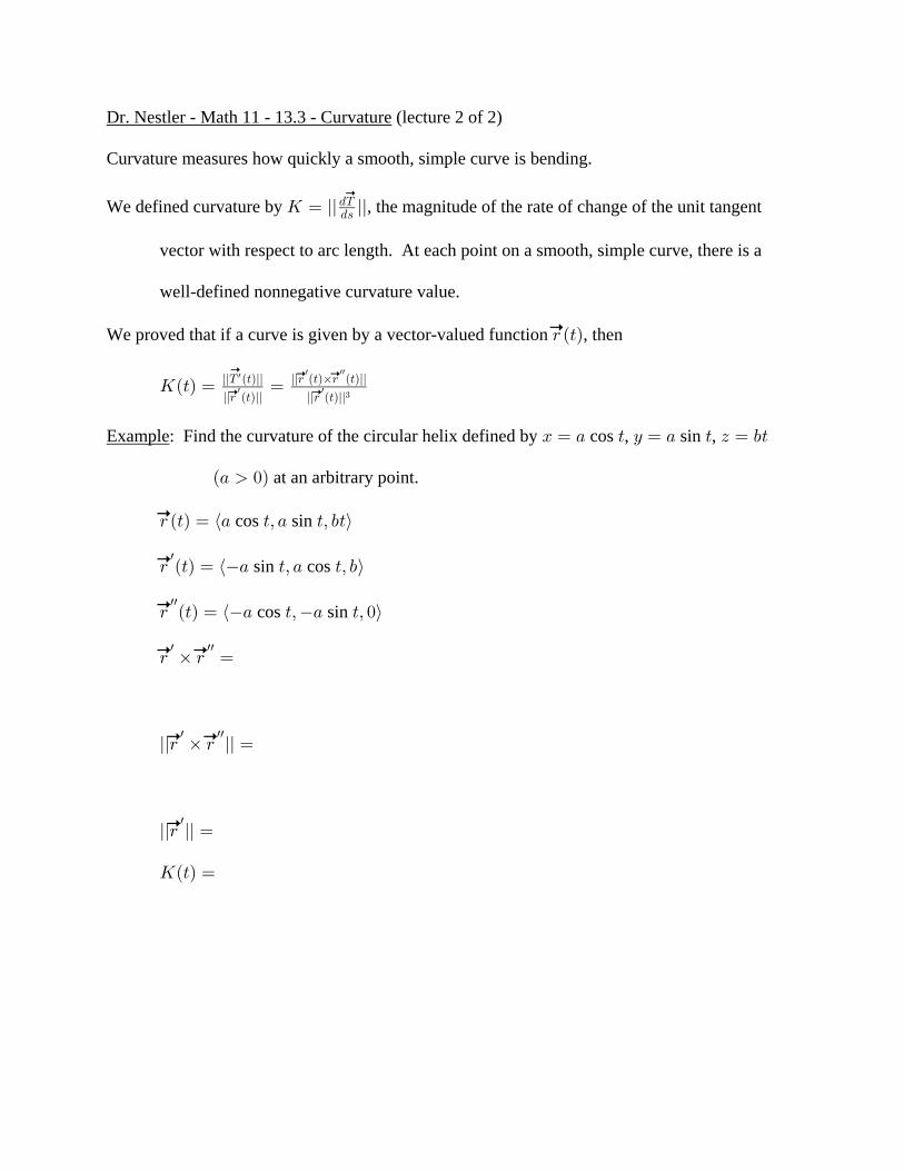
Dr. Nestler - Math 11 - 13.3 - Curvature (lecture 2 of 2)
Curvature measures how quickly a smooth, simple curve is bending.
We defined curvature by , the magnitude of the rate of change of the unit tangentO œ ll ll.Xp
.=
vector with respect to arc length. At each point on a smooth, simple curve, there is a
well-defined nonnegative curvature value.
We proved that if a curve is given by a vector-valued function , then< Ð>Ñp
OÐ>Ñ œ œllX Ð>Ñll ll< Ð>Ñ‚< Ð>Ñllp
ll< Ð>Ñll ll< Ð>Ñllp p
p pw
w w
w ww
$
Example: Find the curvature of the circular helix defined by cos , sin , B œ + > C œ + > D œ ,>
at an arbitrary point.Ð+ !Ñ
cos sin < Ð>Ñ œ Ø+ >ß + >ß ,>Ùp
sin cos < Ð>Ñ œ Ø+ >ß + >ß ,Ùpw
cos sin < Ð>Ñ œ Ø+ >ß+ >ß !Ùpww
< ‚ < œp pw ww
ll< ‚ < ll œp pw ww
ll< ll œpw
OÐ>Ñ œ

Special case (#42): Suppose that is a plane curve with parametric equationsG
, . Then is defined in by vector functionB œ 0Ð>Ñ C œ 1Ð>Ñ G ‘$
< Ð>Ñ œ Ø0Ð>Ñß 1Ð>Ñß !Ùp
< Ð>Ñ œ Ø0 ß 1 ß !Ùpw w w
< Ð>Ñ œ Ø0 ß 1 ß !Ùpww ww ww
< ‚ < œp pw ww
O œ
To help remember this formula, notice that the numerator is the absolute value of this
determinant: 0 10 1
w w
ww ww
Example: Find the curvature of the curve sin , cos at the pointBÐ>Ñ œ > > CÐ>Ñ œ " >
.TÐ "ß "Ñ1#
corresponds to the value T > œ
B Ð>Ñ œ C Ð>Ñ œw w
B Ð>Ñ œ C Ð>Ñ œww ww
OÐ Ñ œ1#
An even more special case: Suppose that is a plane curve with equation .G C œ 1ÐBÑ
Then with parameter , so < ÐBÑ œ ØBß 1ÐBÑß !Ù B OÐBÑ œp
Example: Find the curvature of the parabola at , and .C œ B Ð!ß !Ñ Ð"ß "Ñ Ð#ß %Ñ#
, C œ #B C œ # Ê OÐBÑ œw ww
.

Example: Find the points on the curve at which the curvature is a maximum.C œ /B
C œ / C œ /w B ww B
To maximize the function , we find its criticalOÐBÑ œ œ OÐBÑlC l
"ÐC Ñ
ww
w #$#
points using single-variable calculus:
O ÐBÑ œw Ð"/ Ñ Ð/ Ñ/ † Ð"/ Ñ Ð#/ Ñ
Ð"/ Ñ
#B B B #B #B$ "# #$
##B $ œ !
/ Ð"/ Ñ$/
"/
B #B $B
#B&# œ !
/ #/
"/
B $B
#B&# œ !
/ Ð" #/ Ñ œ !B #B
#/ œ "#B
/ œ#B "#
ln ln ln #B œ œ # œ #"#
"
So the only critical point is B œ
Using the 1st or 2nd derivative test, we can verify that has a maximum at this criticalO
point.
[Can do #27-32, 38, 39, 43-46]


Dr. Nestler - Math 11 - 14.4 - Differentiable Functions [part 1]
Facts from Calculus 1: If a real-valued function is differentiable at a number , then0ÐBÑ +
(1) is continuous at ,0 +
(2) the curve has a nonvertical tangent line at , andC œ 0ÐBÑ Ð+ß 0Ð+ÑÑ
(3) a small change (increment) in near can be approximated using a differential.0 +
Math 11 Goal: Define "differentiable" so that if a function is differentiable at , then0ÐBß CÑ Ð+ß ,Ñ
(1) is continuous at ,0 Ð+ß ,Ñ
(2) the surface has a nonvertical tangent plane at , andD œ 0ÐBß CÑ Ð+ß ,ß 0Ð+ß ,ÑÑ
(3) a small change (increment) in near can be approximated using a differential.0 Ð+ß ,Ñ
Consider the case . If is an increment of , let .C œ 0ÐBÑ B B C œ 0Ð+ BÑ 0Ð+Ñ? ? ?
If is differentiable at , then exists.0 + 0 Ð+Ñ œw
˜BÄ!
˜C˜Blim
Given an increment , let , so is a function of and .? % % ? %B œ 0 Ð+Ñ B œ !??CB
w
˜BÄ!lim
Rewrite as: ??CB
wœ 0 Ð+Ñ %
? % ?C œ Ð0 Ð+Ñ Ñ Bw
Thus where is a function of and as .? % ? % ? % ?C œ Ð0 Ð+Ñ Ñ B B Ä ! B Ä !w
It can be shown that, conversely, the existence of such a number and function is0 Ð+Ñw %
equivalent to the definition of differentiability for .0ÐBÑ
Definitions increment. Let . An of is .D œ 0ÐBß CÑ 0 D œ 0ÐB Bß C CÑ 0ÐBß CÑ? ? ?
The function is at a point in its domain if0 Ð+ß ,Ñdifferentiable
(1) the partial derivatives and exist, and0 Ð+ß ,Ñ 0 Ð+ß ,ÑB C
(2) an increment at can be expressed in the form?D Ð+ß ,Ñ
where and are functions of and? % ? % ? % %D œ 0 Ð+ß ,Ñ B 0 Ð+ß ,Ñ C ˜B B " C # " #
such that , as and approach 0.? % % ? ?C Ä ! B C" #

Example: Show that, according to the definition, the function is differentiable at0ÐBß CÑ œ B C#
each point in the plane.Ð+ß ,Ñ
Theorem. If is differentiable at , then is continuous at .0ÐBß CÑ +ß , 0 Ð+ß ,Ñ : Since is differentiable, given increments and , an increment of atProof 0 B C 0? ?
can be written Ð+ß ,Ñ D œ 0Ð+ Bß , CÑ 0Ð+ß ,Ñ? ? ?
.œ 0 Ð+ß ,Ñ B 0 Ð+ß ,Ñ C B " C #% ? % ?
Let , . ThenB œ + B C œ , C? ?
? % %D œ 0ÐBß CÑ 0Ð+ß ,Ñ œ 0 Ð+ß ,Ñ ÐB +Ñ 0 Ð+ß ,Ñ ÐC ,Ñ B " C #
Now let , so : ÐBß CÑ Ä Ð+ß ,Ñ Bß C Ä ! 0ÐBß CÑ 0Ð+ß ,Ñ œ !? ? limÐBß CÑÄÐ+ß ,Ñ
So , as desired.limÐBß CÑÄÐ+ß ,Ñ
0ÐBß CÑ œ 0Ð+ß ,Ñ

Theorem. If and exist in an open disk containing and are continuous at , then 0 0 Ð+ß ,Ñ Ð+ß ,Ñ 0B C
is differentiable at . +ß ,
: Next lecture. See also Appendix F.Proof
Example: Prove that is differentiable on its domain.0ÐBß CÑ œ BCC B# #
Example: We can show that the function has first partialif , otherwise
0ÐBß CÑ œ" B C !!
derivatives at the origin, but the function is not continuous there, and so it is not differentiable there.
The next example shows that the converse of the first theorem above is false.
Example: We can show that the function is continuous at the origin,D œ 0ÐBß CÑ œ B C # #
but the function does not have first partial derivatives there, and so it is not differentiable there.
[Can do #11-16 "Explain why the function is differentiable at the given point," 43, 44, 46]

Dr. Nestler - Math 11 - 14.4 - Differentiable Functions (Part 2)
Thm. Let be a function of two variables. If and exist in an open disk containing0ÐBß CÑ 0 0B C
a point and they are continuous at , then is differentiable at .Ð+ß ,Ñ +ß , 0 +ß , Proof: An increment of at is . We mustD œ 0ÐBß CÑ Ð+ß ,Ñ D œ 0Ð+ Bß , CÑ 0Ð+ß ,Ñ? ? ?
show that we can write this in the form ? % ? % ?D œ 0 Ð+ß ,Ñ B 0 Ð+ß ,Ñ C B " C #
where the functions , as , . We can write the increment as a sum% % ? ?" # Ä ! B C Ä !
(*) ? ? ? ? ?D œ 0Ð+ Bß , CÑ 0Ð+ß , CÑ 0Ð+ß , CÑ 0Ð+ß ,Ñ For simplicity, assume , .? ?B C !
Let , which is the function with the -component of its domain1 B œ 0ÐBß , CÑ 0 C ?
restricted to the value . For small enough and , the single-variable function, C B C? ? ?
1ÐBÑ Ò+ß + BÓ 1 ÐBÑ œ 0 ÐBß , CÑ is differentiable on the interval , and . (The size of the? ?wB
increments and is determined by the size of the disk in which the first partials of ? ?B C 0
exist.) By the Mean Value Theorem, for some number1Ð+ BÑ 1Ð+Ñ œ 1 Ð?Ñ B? ?w
? − Ð+ß + BÑ? . Thus the first part of the sum (*) is
0Ð+ Bß , CÑ 0Ð+ß , CÑ œ 0 Ð?ß , CÑ B? ? ? ? ?B
Similarly, the function is differentiable on for small enough2ÐCÑ œ 0Ð+ß CÑ Ò,ß , CÓ?
increments, and . By the Mean Value Theorem, 2 ÐCÑ œ 0 Ð+ß CÑ 2Ð, CÑ 2Ð,Ñ œ 2 Ð@Ñ Cw wC ? ?
for some number . Thus the second part of the sum (*) above is@ − Ð,ß , CÑ?
0Ð+ß , CÑ 0Ð+ß ,Ñ œ 0 Ð+ß @Ñ C? ?C

Rewrite (*) using (1) and (2):
? ? ? ?D œ 0 Ð?ß , CÑ B 0 Ð+ß @Ñ CB C
.œ 0 Ð+ß ,Ñ 0 Ð?ß , CÑ 0 Ð+ß ,Ñ B 0 Ð+ß ,Ñ 0 Ð+ß @Ñ 0 Ð+ß ,Ñ C B B B C C C? ? ?
As and , and , and so and since , are? ? % %B Ä ! C Ä ! ? Ä + @ Ä , Ä ! Ä ! 0 0" # B C
continuous at . Thus is differentiable at . Ð+ß ,Ñ 0 Ð+ß ,Ñ
Notes:
1. There is a stronger result that says if both first partial derivatives are defined in an open disk
containing the point and if at least one of them is continuous at the point, then the function must
be differentiable at the point.
2. The converse of the theorem is false. See the class homepage for an example of a
differentiable function with discontinuous first partial derivatives.


Math 11 - Dr. Nestler - Review of Definite Integrals from Math 7 (Calculus 1)
Definitions. Suppose a function is continuous on a closed interval . Divide into 0 Ò+ß ,Ó Ò+ß ,Ó 8
subintervals of equal length , and choose a number ( ) inÒB ß B Ó B A3" 3 3? sample point
for each . The expression is called a ÒB ß B Ó 3 œ "ßá ß 8 0ÐA Ñ B3" 3 33œ"
8 ? Riemann sum
for on . If it exists, the number is called the 0 Ò+ß ,Ó 0ÐA Ñ Blim8Ä∞ 3œ"
8
3 ? definite integral
of on , denoted by , and we say is on .0 Ò+ß ,Ó 0ÐBÑ .B 0 Ò+ß ,Ó+, integrable
Theorem. If is continuous on , then is integrable on .0 Ò+ß ,Ó 0 Ò+ß ,Ó
If is continuous and nonnegative on , then equals the area under the graph of0 Ò+ß ,Ó 0ÐBÑ .B+,
from to .C œ 0ÐBÑ + ,
Fundamental Theorem of Calculus: Each continuous function on a closed interval has an0 Ò+ß ,Ó
antiderivative on , and .J Ò+ß ,Ó 0ÐBÑ .B œ JÐ,Ñ JÐ+Ñ+,


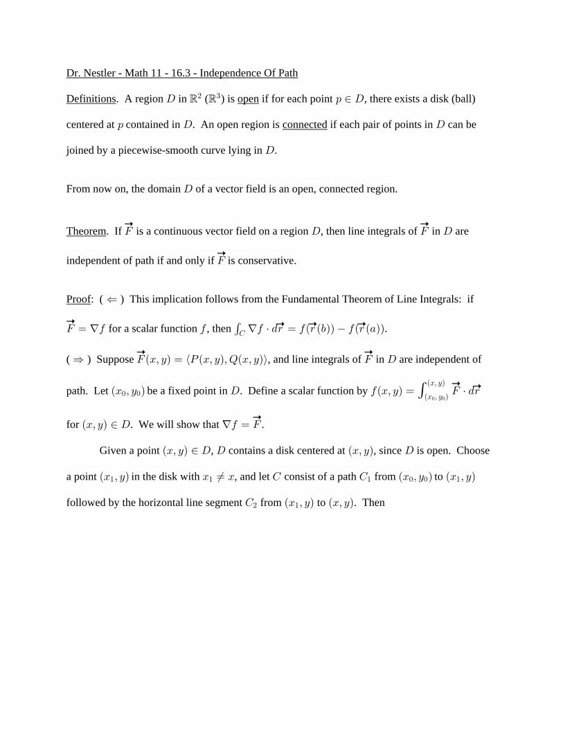
Dr. Nestler - Math 11 - 16.3 - Independence Of Path
Definitions open. A region in ( ) is if for each point , there exists a disk (ball)H : − H‘ ‘# $
centered at contained in . An open region is if each pair of points in can be: H Hconnected
joined by a piecewise-smooth curve lying in .H
From now on, the domain of a vector field is an open, connected region.H
Theorem. If is a continuous vector field on a region , then line integrals of J J Hp p
H in are
independent of path if and only if is conservative.Jp
Proof: ( ) This implication follows from the Fundamental Theorem of Line Integrals: ifÉ
J œ f0 0 f0 † .< œ 0Ð< Ð,ÑÑ 0Ð< Ð+ÑÑp p p p for a scalar function , then .
G
( ) Suppose , and in are independent ofÊ JÐBß CÑ œ ØT ÐBß CÑßUÐBß CÑÙ J Hp p
line integrals of
path. Let be a fixed point in . Define a scalar function by ÐB ß C Ñ H 0ÐBß CÑ œ J † .<p p
! ! ÐB ß C Ñ
ÐBß CÑ! !
for . We will show that .ÐBß CÑ − H f0 œ Jp
Given a point , contains a disk centered at , since is open. ChooseÐBß CÑ − H H ÐBß CÑ H
a point in the disk with , and let consist of a path from to ÐB ß CÑ B Á B G G ÐB ß C Ñ ÐB ß CÑ" " " ! ! "
followed by the horizontal line segment from to . ThenG ÐB ß CÑ ÐBß CÑ# "

0ÐBß CÑ œ J † .< J † .< œ J † .< J † .<p p p pp p p p
G G GÐB ß C Ñ
ÐB ßCÑ
" # #! !
"Differentiate both sides with respect to :B
`0`B `B `B` `
ÐB ß C Ñ
ÐB ßCÑ
Gœ J † .< J † .<p pp p
! !
"
#
`0`B `B`
Gœ J † .<p p
#
On , is constant so is . Rewrite the previous equation using the component formG C .C !#
of the line integral:
`0`B `B
`Gœ T .B U.C
#
by the Fundamental Theorem of Calculus.œ TÐ>ß CÑ .> œ TÐBß CÑ``B B
B "
Similarly, we could show , using a vertical line segment instead of a horizontal`0`C œ UÐBß CÑ
one. Thus , as desired. J œ ØT ßUÙ œ Ø0 ß 0 Ù œ f0p
B C


Dr. Nestler - Math 11 - 16.8 - Proof of a special case of the Stokes Theorem
Suppose the surface W D œ 1ÐBß CÑ ÐBß CÑ H 1 is the graph of with in a plane region , and has
continuous 2nd partials. If is oriented upward, then theW
positive orientation of corresponds to the positive orientation ofG
its projection , the boundary of . Let , beG H ØBÐ>Ñß CÐ>ÑÙ > − Ò+ß ,Ó"
a parametrization of . Then ,G BÐ>Ñß CÐ>Ñß 1 BÐ>Ñß CÐ>Ñ" > − Ò+ß ,Ó G J œ ØT ßUßVÙ
p is a parametrization of . Let be a vector field whose component
functions have continuous 1st partials on a region containing . ThenW
(1) G +
, wJ † .< œ JÐ< Ð>ÑÑ † < Ð>Ñ .>p pp p p
(2) œ T U V .> +, .B `D .B `D
.> .> `B .> `C .>.C .C
(3) œ T V UV .> +, `D .B `D
`B .> `C .>.C
(4) œ T V .B UV .C G
`D `D`B `C"
(5) œ UV T V .EH
` `D ` `D`B `C `C `B
(6) œ U U V V VH
B D B D`D ` D `D `D `D`B `B`C `C `B `C
#
T T V V V .E C D C D`D ` D `D `D `D`C `C`B `B `C `B
#
(7) œ ÐV U Ñ ÐT V Ñ ÐU T Ñ .EH
C D D B B C`D `D`B `C
(8) œ ØV U ßT V ßU T Ù † Ø ß ß "Ù .EH
C D D B B C`D `D`B `C
(9) curl .œ J † 8 .WW
p p


Dr. Nestler - Math 11 - 16.8 - Conservative Vector Fields
Theorem. Given a vector field with continuous first partial derivatives on a simply connectedJp
domain , the following are equivalent:H
(1) is conservative.Jp
(2) Line integrals of are independent of path.Jp
(3) for all closed curves .G J † .< œ ! Gp p
(4) The cross partial derivatives of are equal.Jp
(5) is irrotational.Jp
Proof: We proved (1) (2) (3) and (1) (4).Í Í Í
(1) (5): proved on p. 1144 in 16.5.Ê
(5) (3): This is a corollary of the Stokes Theorem. If is a simple closed smoothÊ G
curve in , then an advanced theorem states that is the boundary of a smooth orientedH G
surface in . By the Stokes Theorem, curl .W H J † .< œ Ð J Ñ † .W œ ! .W œ !p pp
W W
p p G
Note: Implications (4) (1) and (5) (1) require the simple connectivity of the domain.Ê Ê

Related Documents