DP1

Dynamic Programming: Part 1 Classical

Algorithms

Wilan [email protected]

1

Contents

1 Introduction 3

2 Fibonacci Sequence 3

3 The Knapsack Problem 8

3.1 Introduction . . . . . . . . . . . . . . . . . . . . . . . . . . . . . . 8

3.2 Modelling a Dynamic Programming Algorithm . . . . . . . . . . 10

3.3 Other Knapsack variants . . . . . . . . . . . . . . . . . . . . . . . 15

4 Edit Distance 18

4.1 Modelling and Implementation . . . . . . . . . . . . . . . . . . . 18

4.2 Performance Differences . . . . . . . . . . . . . . . . . . . . . . . 23

5 Overview 25

6 Problems 25

6.1 Problem 1: Longest Increasing Subsequence . . . . . . . . . . . . 25

6.2 Problem 2: Binomial Coefficients . . . . . . . . . . . . . . . . . . 26

6.3 Problem 3: Longest Common Subsequence . . . . . . . . . . . . . 27

6.4 Problem 4: Handshaking Problem . . . . . . . . . . . . . . . . . 28

2

1 Introduction

Dynamic programming is one of the major techniques used within combinato-rial optimisation. Combinatorial optimisation algorithms solve problems thatare believed to be hard in general, by searching the large solution space of theseproblems. However, due to the large solution space many problems become toounwieldy to be solve with brute force based algorithms, so combinatorial op-timisation algorithms achieve better performance by reducing the search spaceby discarding portions of the solution space that can be deemed non-optimal,these algorithms also usually explore the space efficiently so they don’t recal-culate identical problems. Simply put, dynamic programming is a method toexploit inherit properties of a problem, so the algorithm runs much faster thansimpler straightforward brute-force algorithms.

The basis behind dynamic programming is what’s known as a functional equa-tion. You can think of this as some sort of recurrence relation which relates theproblem we are trying to solve with smaller subproblems of the same problem.This in effect, means that dynamic programming is recursive in nature – a solidunderstanding of recursion is required to understand dynamic programmingeven in it’s most basic form. There consists of many deep mathematical theo-ries behind dynamic programming, so we will only consider the fundamentalswhose coverage should be sufficient enough for you to develop a basic dynamicprogramming formulation skill. We now cover basic recursion skills, show it’slimitations when used naively and consequently provide a simple method totranslate recursion to top-down dynamic programming.

2 Fibonacci Sequence

Let us consider a trivial problem that you probably already know of: Fibonaccinumbers. If you haven’t seen Fibonacci numbers before, basically it’s a sequenceof numbers where the next term is defined by the sum of the previous two terms.You start off with the first two terms being 1, so the sequence looks like: 1, 1,2, 3, 5, 8, 13, 21 etc. The goal of this problem is to compute the n-th Fibonaccinumber, so the first Fibonacci number would be 1, the third would be 2, thesixth would be 8 and so on.

How do we formulate a recursive algorithm for this problem? Let’s assume weknow all Fibonacci numbers up to the (n-1 )th term, now we ask ourselves howdo we obtain the n-th term. If we knew all the Fibonacci numbers up to the(n-1 )th one then by the definition of a Fibonacci sequence: Fn = Fn−1 + Fn−2

we can calculate the next one. This itself forms the basis of the recursion, itdefines the current problem (Fn) in terms of two smaller subproblems (Fn−1

and Fn−2) in which they are related by the addition of the two subproblems.As you may know from recursion – it is crucial to have a base case, and the

3

recursion itself should move closer and closer to this base case otherwise it mightnot terminate for certain inputs.

So our second task after defining the recurrence relation (Fn = Fn−1 + Fn−2) isto determine suitable “stopping” conditions (or base cases). Since the recurrencerelation relies on the previous two terms – we must provide at least 2 consecutivebase cases otherwise the relation would be undefined. If we look back at thesequence we see that the first two terms are just 1. So we can define F0 = F1 = 1as the base case.

Looking back we can formally define our functional or recursive equation as:

F (n) ={

1 if n = 0, 1F (n− 1) + F (n− 2) otherwise

Now, we simply just translate the above to a programming language. We willbe demonstrating our algorithms in C++ for this tutorial, most readers shouldhave little difficulty transferring it to their preferred language of choice. SeeListing 1 for the implementation.

Listing 1: Fibonacci Naive Recursion Approach1 #include <iostream>23 using namespace std ;45 long long f i b ( int n) {6 i f (n <= 1) return 1 ;7 return f i b (n−1)+ f i b (n−2);8 }9

10 int main ( ) {11 int n ;12 while ( c in >> n) cout << f i b (n) << "\n" ;13 return 0 ;14 }

The first thing to note if you have compiled and ran this algorithm, is that it getsvery slow for even modest sized inputs. One thing that may come to mind is thatrecursion is just plain slow – or is it? Certainly, there is additional overhead forrecursion due to stack modifications for function calls (i.e. pushing and poppingoff local and function parameters on the stack) – however it certainly shouldn’thave an exponential impact. If we draw out the recursion tree of the Fibonaccinumbers, we yield the source of our problem. The problem lies with multiplecalls to the same functions that we have already calculated previously – thediagram below illustrates this better.

4

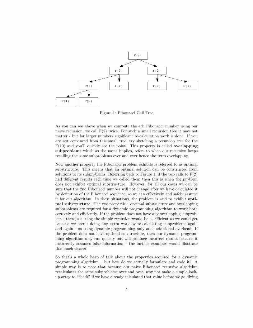
Figure 1: Fibonacci Call Tree

As you can see above when we compute the 4th Fibonacci number using ournaive recursion, we call F(2) twice. For such a small recursion tree it may notmatter - but for larger numbers significant re-calculation work is done. If youare not convinced from this small tree, try sketching a recursion tree for theF(10) and you’ll quickly see the point. This property is called overlappingsubproblems which as the name implies, refers to when our recursion keepsrecalling the same subproblems over and over hence the term overlapping.

Now another property the Fibonacci problem exhibits is referred to as optimalsubstructure. This means that an optimal solution can be constructed fromsolutions to its subproblems. Referring back to Figure 1, if the two calls to F(2)had different results each time we called them then this is when the problemdoes not exhibit optimal substructure. However, for all our cases we can besure that the 2nd Fibonacci number will not change after we have calculated itby definition of the Fibonacci sequence, so we can effectively and safely assumeit for our algorithm. In these situations, the problem is said to exhibit opti-mal substructure. The two properties: optimal substructure and overlappingsubproblems are required for a dynamic programming algorithm to work bothcorrectly and efficiently. If the problem does not have any overlapping subprob-lems, then just using the simple recursion would be as efficient as we could getbecause we aren’t doing any extra work by re-calculating subproblems againand again – so using dynamic programming only adds additional overhead. Ifthe problem does not have optimal substructure, then our dynamic program-ming algorithm may run quickly but will produce incorrect results because itincorrectly assumes false information – the further examples would illustratethis much clearer.

So that’s a whole heap of talk about the properties required for a dynamicprogramming algorithm – but how do we actually formulate and code it? Asimple way is to note that because our naive Fibonacci recursive algorithmrecalculates the same subproblems over and over, why not make a simple look-up array to “check” if we have already calculated that value before we go diving

5

further into the recursion tree? So this logically works by having a “special”value that denotes that we have not calculated that problem before (usuallynegative numbers but may change depending on the nature of the problem),then for the recursive function, we check if the current value in the look-uparray corresponding to the function input is equal to the “special” value. If itis, then we know that it still hasn’t been calculated, otherwise if it isn’t, thenwe already know the result of that input – and we can just return the value ofthe look-up array in that specific index. It may sound complex, but augmentingit is relatively easy and is usually universal across many dynamic programmingalgorithms. (See Listing 2 for implementation)

Listing 2: Fibonacci Memoization Approach1 #include <iostream>23 using namespace std ;45 #define MAXTERMS 10067 long long memo[MAXTERMS+1] ;89 long long f i b ( int n) {

10 i f (n <= 1) return 1 ;11 i f (memo[ n ] != −1) return memo[ n ] ;12 return memo[ n ] = f i b (n−1) + f i b (n−2);13 }1415 int main ( ) {16 int n ;17 memset (memo,−1 , s izeof (memo) ) ;18 while ( c in >> n && n <= MAXTERMS) cout << f i b (n) << "\n" ;19 return 0 ;20 }

You should compare the running times between our first attempt and after weapplied a caching mechanism to the recursion. In fact, there’s an exponentialdifference in running time between the two algorithms even though they arefundamentally similar. Also note, that you will need to use arbitrary-precisionintegers very soon above the Fibonacci term of 100 because the numbers growthquickly and exceed the 64-bit integer data-type limit.

You may have coded another iterative algorithm for the Fibonacci sequencebefore in an introduction to programming course (see Listing 3), which is tokeep track of the last two terms and keep generating the next term based on afor-loop or a similar construct. In effect, that method is dynamic programming –it differs in the order of execution because it approaches the problem bottom-up,i.e. it solves the simplest cases first and gradually builds up to larger cases. The

6

Listing 3: Fibonacci Iterative Variant1 #include <iostream>23 using namespace std ;45 int main ( ) {6 int n ;7 while ( c in >> n) {8 i f (n <= 1) {9 cout << "1\n" ;

10 continue ;11 }12 long long prev = 1 , prev2 = 1 ;13 for ( int i = 2 ; i <= n ; i++) {14 long long temp = prev ;15 prev += prev2 ;16 prev2 = temp ;17 }18 cout << prev << "\n" ;19 }20 return 0 ;21 }

recursion + look-up method is called memoization and is also known as top-downdynamic programming, it’s called top-down because it seeks to “solve” largerinstances of the problem first and gradually moves down until it hits the basecases (which are usually the simplest cases of the problem). Both methods havesimilar run-time performance but there are subtle differences to note. Bottom-up is usually considered more efficient because it doesn’t have the stack overheadof recursive algorithms, however memoization does have an advantage in that itonly calculates the subproblems that it needs whereas bottom-up needs to solveall of the subproblems up to the current input.

It’s somewhat easier to learn dynamic programming using the top-down ap-proach because when you use bottom-up dynamic programming you have toensure the order in which you calculate the subproblems is correct (i.e. youhave to make sure you have already calculated all the required subproblemswhen you reach a given problem) otherwise the whole dynamic programmingapproach breaks up. Top-down dynamic programming achieves this implicitlythrough the recursive call structure so you only need to worry about setting upthe recursive algorithm. That being said, all top-down dynamic programmingalgorithms can be converted to bottom-up and vice versa. Nevertheless, we willcover bottom-up dynamic programming in our next problem which is slightlymore complicated than the one we have seen so far.

7

3 The Knapsack Problem

3.1 Introduction

Let’s consider a more complex example than the Fibonacci problem discussedpreviously. The next problem we will be looking at is called the Knapsackproblem. It’s a classic Computer Science problem which entails the following:

You’re a thief that has successfully infiltrated inside a bank. However to yoursurprise there are only items of questionable value as opposed to money. Youbought a bag that can only hold a certain weight (W), you want to pack itemsinto the bag so that you collect the best possible value of items whilst notpacking more than the limit of W. Each item has a weight and a value. Yourtask would be to return the highest value you can get from this bank robbery.

An intuitive approach might be to pack items by the best value per weightratio until the bag is full or cannot hold anymore items. This is called a greedyalgorithm, in which each decision stage you choose the most locally optimalchoice (i.e. in this case, the best value/weight ratio that hasn’t been taken andalso fits in the bag). However, without a correctness proof we wouldn’t be sureit would work for all cases. In fact, this greedy strategy does not work for theknapsack problem in general. How do we show this? We simply need to find acounter-example.

Let’s consider an example, where the greedy strategy does indeed get the optimalsolution:

Bag Weight (W) = 10 kgsItem Configurations (Weight, Value) Pairs: (5,5), (3,2), (1,0),(10,6), (8,5)

Using the greedy strategy, we first calculate all the value per weight ratios.These are listed as:

Item Configuration Ratios: 1.0, 0.66, 0.0, 0.6, 0.625

respectively. Now we begin to pack the items. Keep in mind, there are differentvariations of the Knapsack problem, one variation is that there is an unlimitednumber of items of each type, and another variation consists of only allowing alimited amount of each type of item. We will consider the unlimited variationfirst and later discuss on the limited version. Now back to the greedy strategy,we see that the item of 5kg and value of $5 is the best in terms of ratio. Wepack one of them inside our bag, we have 5kgs remaining and we repeat thesame process (huge hint for recursion). Again we choose the same item type

8

because it can still fit, now we have 0kg remaining – so we halt. In the end, wechose 2 items of (5,5) which gave us a total value of $10. Convince yourself thisis the best you can get from any combination of the items. Does this mean thatour greedy strategy works? The simple answer, no!

Let’s consider an example that breaks the intuitive strategy,

Bag Weight (W) = 13 kgsItem Configurations (Weight, Value) Pairs: (10,8), (8,6), (5,3),(10,6), (1,0)Item Configuration Ratios: 0.8, 0.75, 0.6, 0.6, 0.0

If we repeat the same process again, we end up choosing 1 x (10,8) because it hasthe highest ratio. So we are left with 3kg, however none of the items fit (exceptfor 3 x (1,0) which gives a value of $0). So the best value we can get from ourgreedy approach is $8. However, you can observe that you can get $9 of valuefrom a combination of (8,6) and (5,3). Hence, this works as a counter-exampleagainst our greedy strategy and hence the greedy algorithm isn’t correct.

So how else can we approach this problem? One sure way to get a correct answerwould be to brute force every single item configuration, check if it fits insidethe bag and update it if it’s better than the current maximum. However, it’shorribly inefficient to do it this way. A very naive approach based on this wouldbe to generate subsets of items and test each one, however as you may know thenumber of subsets in a set is exponential (2n). In fact, this problem is classifiedas NP-hard which means the best way we currently know how to do it is in ex-ponential time (without getting too rigorous). However, dynamic programmingprovides a pseudo-polynomial time algorithm that correctly solves the Knapsackproblem. It’s important to distinguish between a “pseudo-polynomial” time al-gorithm and a polynomial algorithm. Loosely speaking, a polynomial algorithmis one where it’s time complexity is bounded by a constant power that isn’trelated to the input numerical values (not sizes) in any way – examples wouldbe O(n2), O(n3), O(n100).

A “pseudo-polynomial” time algorithm grows in proportion to the input’s nu-merical value, so for example O(nm) would be a pseudo-polynomial time com-plexity if either n and m are related to the input’s numercial values. For ex-ample, if an algorithm runs in O(nm) where m is some constant and n variedwith the largest input value, then the algorithm would be pseudo-polynomial.However, if the input values remain fairly small – then the overall algorithm isstill efficient. A dynamic programming Knapsack algorithm belongs to such aclass as we will see shortly.

9

3.2 Modelling a Dynamic Programming Algorithm

However how do we approach this problem in a dynamic programming way?There are a few basic general guidelines used when formulating any dynamicprogramming algorithm:

1. Specify the state

2. Formulate the functional/recursive equation in terms of the state

3. Solve/code the solution using Step 2

4. Backtrack the solution (if necessary)

Step 1: Specifying the stateA state is simply information that we need in each step of the recursion tooptimally decide and solve the problem. In the Fibonacci example, the state wassimply the term number – this alone allowed us to decide what the subproblemswere and if they were base cases or not. For this example, it isn’t as easy tocome up with. In fact, for most dynamic programming algorithms coming upwith a suitable and efficient state is the hardest part.

For the Knapsack problem, when we try to look for the state – a good indicatoris what the recursion function parameters would look like. For simple problems,you can solely base your state on these, however for more complex problemswhere the state space can be huge – you will need to do some fancy tricksand optimisations to ensure the state is as condensed as possible whilst stillrepresenting the problem in a correct fashion.

So ask yourself, what are the common links between a specific problem and itssubproblems? The knapsack subproblems were simply ones where the weightremaining was smaller. All the other factors remained the same (the availablechoice of items). Can we base our state solely on the weight? When you askyourself this, just think if someone gave you a single parameter (the weight) anda list of possible items, could you decide the optimal decision to choose assumingyou know the optimal values of all the weights beneath it? The answer to thisis, yes! Thinking recursively is usually the best strategy, for example, if we weregiven a weight W to fill in the bag and we knew the best values we could getfrom weight 0 up to W − 1, then a simple method would be to iterate througheach of the lesser weights and try adding the best item to it so it can exactly fillweight W . We then choose the greatest value of these configurations. Convinceyourself this is sufficient by drawing some examples – this is one of the two mainproperties of dynamic programming: optimal substructure.

Step 2: Formulating the recursive equationNow we have a state which in this case is just weight remaining in the bag.We need to build a recursive relationship between states, i.e. link up a state to

10

another state. Usually this is obvious because it works in one direction: towardsthe base case. The base case for our problem would simply be the weight of0. We realistically assume you cannot fit anything in a bag that can’t storeanything – hence the value of a bag weight of 0 is just simply 0. Since we areworking towards this goal, we want recursive calls to generate successively lowerweights.

To determine a relationship between the states we take note that, we can adda single item at a time since order does not matter. So we can relate a lowerweight state by adding items so it becomes exactly W . To determine whichlower weight states are relevant, we just iterate through the item list of weightsand subtract it from W , i.e. W −Wi (where Wi is the weight of item i). Ifthis value is less than 0 obviously we don’t want it because that would violatethe weight constraints (you are storing a heavier item than what could fit inthe remaining bag). So we simply choose the best out of these item additions.Hence the recurrence/functional equation may look like:

F (w) ={

max {F (w − wi) + vi} if w − wi ≥ 0, ∀i in items0 if w = 0

What do we initialise F (w) before we begin comparisons? One option would beto set it to 0 – however if we were to do this then we need to loop through allweight values at the end and choose the maximum. Another option would be toset F (w) to be equal to F (w− 1) initially – this makes sense because if an itemconfiguration can fit in w−1 then it should be able to fit in w, doing it this waysaves us having to loop through all the weight values at the end. Either optionproduces the correct output, so it’s just a matter of taste. Another alternativewould be to add a “dummy” item with weight 1 and value 0 - this implicitlysets F (w) to be at least as much as F (w − 1).

So for step 2, we have the slightly modified recursive definition:

F (w) ={

0 if w = 0max {F (w − wi) + vi, F (w − 1)} if w − wi ≥ 0, ∀i in items

The recursion implies that F (w) should be set to F (w − 1) value without theneed to fulfill the w − wi ≥ 0 requirement.

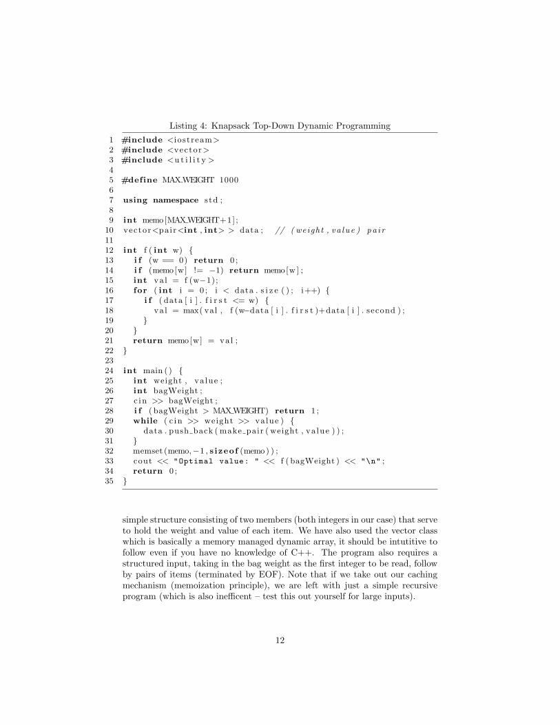
Step 3: Coding the recursion equationCoding the recursive algorithm is usually fairly straightforward and simple. AC++ memoized solution is shown in Listing 4.

If you look at the source code and compare it with our original recurrenceformulation in step 2, you will see there are a lot of similarities in the recursivefunction f(). For non-C++ users, we have used a pair class which is basically a

11

Listing 4: Knapsack Top-Down Dynamic Programming1 #include <iostream>2 #include <vector>3 #include <u t i l i t y >45 #define MAXWEIGHT 100067 using namespace std ;89 int memo[MAXWEIGHT+1] ;

10 vector<pair<int , int> > data ; // ( weight , va lue ) pa i r1112 int f ( int w) {13 i f (w == 0) return 0 ;14 i f (memo[w] != −1) return memo[w ] ;15 int va l = f (w−1);16 for ( int i = 0 ; i < data . s i z e ( ) ; i++) {17 i f ( data [ i ] . f i r s t <= w) {18 va l = max( val , f (w−data [ i ] . f i r s t )+data [ i ] . second ) ;19 }20 }21 return memo[w] = va l ;22 }2324 int main ( ) {25 int weight , va lue ;26 int bagWeight ;27 c in >> bagWeight ;28 i f ( bagWeight > MAXWEIGHT) return 1 ;29 while ( c in >> weight >> value ) {30 data . push back ( make pair ( weight , va lue ) ) ;31 }32 memset (memo,−1 , s izeof (memo) ) ;33 cout << "Optimal value: " << f ( bagWeight ) << "\n" ;34 return 0 ;35 }

simple structure consisting of two members (both integers in our case) that serveto hold the weight and value of each item. We have also used the vector classwhich is basically a memory managed dynamic array, it should be intutitive tofollow even if you have no knowledge of C++. The program also requires astructured input, taking in the bag weight as the first integer to be read, followby pairs of items (terminated by EOF). Note that if we take out our cachingmechanism (memoization principle), we are left with just a simple recursiveprogram (which is also inefficent – test this out yourself for large inputs).

12

You can see from the implementation above, there is a limitation of dynamicprogramming. What happens if the weight of 1 item was as large as 1 billion?We would have to make a caching array of 1 billion integers representing each ofthe weights that are possible. Now we have a memory limit situation - this algo-rithm doesn’t scale well to large value inputs! We also have an execution timeproblem, in the worst case we have to recurse through 1 billion f() recursivefunctions (which will definitely overflow the stack before it finishes it’s calcu-lations). The point is that dynamic programming isn’t a silver bullet for hardproblems – it only runs well under limited conditions. So you should definitelycheck whether the state space is too large before you begin formulating/codingthe problem!

Step 4: Backtrack the solutionsIt’s all nice and good to know the best value we can get from the knapsackproblem. However, the thief still scratches his head because although he knowsthe best value he can come out with, what items should he actually choose toobtain the optimal value? It’s important to realise whether you need this step ornot, if you do – then you may need to take additional measures when you codethe recursive algorithm. After the memoization has finished, we know have anarray that details the optimal value for many different weights – we need to usethis (and usually some other bookkeeping information) to backtrack the itemswe have used to get there.

How do we do this? At the moment it contains neither “markers” nor anybookkeeping to allow us to deduce which items where added at each stage ofthe dynamic programming process. So we need to change our implementationto do this.

What markings do we need? We need some way to know which subproblemproduced the best result for a particular weight w, and we need to know whichitem was added on top of that subproblem. To no surprise, this backtracking isalso recursive in nature, you start off at the weight W (the bag weight), assumewe know which item was added and which was the optimal subproblem, then weprint out the item that was added and recurse to the optimal subproblem andrepeat the process until we reach weight 0. The source code below demonstratesthis approach using an extra integer auxiliary array that keep track of whichitem was added (the index of the item) – we can directly deduce the weight ofthe subproblem since we know the weights of each item, we just need to subtractthe item weight off the current weight. You can store it in an array instead ofprinting it, or do other processing – it’s entirely up to you. See Listing 5 and 6for implementation details.

13

Listing 5: Knapsack Top-Down Dynamic Programming with Backtracking1 #include <iostream>2 #include <vector>3 #include <u t i l i t y >45 #define MAXWEIGHT 100067 using namespace std ;89 int memo[MAXWEIGHT+1] ;

10 vector<pair<int , int> > data ; // ( weight , va lue ) pa i r11 int indexTable [MAXWEIGHT+1] ; // used f o r back t r a c k ing12 vector<int> itemsUsed ; // used f o r back t r a c k ing1314 int f ( int w) {15 i f (w == 0) return 0 ;16 i f (memo[w] != −1) return memo[w ] ;17 int va l = f (w−1);18 for ( int i = 0 ; i < data . s i z e ( ) ; i++) {19 i f ( data [ i ] . f i r s t <= w) {20 int k = f (w−data [ i ] . f i r s t )+data [ i ] . second ;21 i f ( va l < k ) {22 va l = k ;23 indexTable [w] = i +1; // bookkeep ing in format ion24 }25 }26 }27 return memo[w] = va l ;28 }2930 void backtrack ( int w) {31 i f (w == 0) return ;32 itemsUsed . push back ( indexTable [w ] ) ;33 backtrack (w − data [ indexTable [w] −1 ] . f i r s t ) ;34 }3536 int main ( ) {37 int weight , va lue ;38 int bagWeight ;39 c in >> bagWeight ;40 i f ( bagWeight > MAXWEIGHT) return 1 ;41 while ( c in >> weight >> value ) {42 data . push back ( make pair ( weight , va lue ) ) ;43 cout << "Item: " << data . s i z e ( ) << " Weight: " <<44 weight << " Value: " << value << "\n" ;45 }

14

Listing 6: Knapsack Top-Down Dynamic Programming with Backtracking (con-tinued)

46 memset (memo,−1 , s izeof (memo) ) ;47 cout << "Optimal value: " << f ( bagWeight ) << "\n" ;48 backtrack ( bagWeight ) ;49 cout << "Items Used:\n" ;50 for ( int i = 0 ; i < itemsUsed . s i z e ( ) ; i++) {51 cout << "Item " << itemsUsed [ i ] << "\n" ;52 }53 return 0 ;54 }

3.3 Other Knapsack variants

Now we have a dynamic programming algorithm that completely solves theknapsack problem. Or have we? Let’s consider another variant where the itemscannot be re-used. How do we keep track of which items have been used ina concise manner? Informally, many people call the knapsack variant we justcompleted a 1 dimensional dynamic programming algorithm. This is becausethe state lies in a 1D state array (the weight). The variant we consider now isin fact, a 2 dimensional dynamic programming algorithm. This should serve asa hint in what the state would be!

If you haven’t guessed it, the state for this variant is (weight, item). How doesthis work? Instead of keeping track whether or not we have used an item ornot, we implicitly enforce the rule by iteratively considering a growing set ofavailable items. For example, if we were given 8 items to pack, we then startoff by considering the first item. Calculate the optimal values for each of theweights for this item. Then we expand to the second item, we use the valuesfor the first item to decide optimal values for each of the weights including thisitem. By “including” this item, we really mean introducing it to the decisionspace – we can actually choose to reject this item if it proves non-optimal.

More formally we can set the state to be equal to:

Let S(W,I) = the optimal value of a bag of weight W using item 1up to item I.

We build the recurrence relation by using the binary (two) decisions we havewhen we “include” an item – do we include it or do we reject it? If we include theitem i then we effectively consume wi worth of weight, if we choose not to includethe item then we don’t consume any weight. However we need to consider thebase cases for the recurrence relation. We can re-use our previous base casewhere any w = 0 has a value of 0. Also if we choose to use 0 items or have 0 items

15

left to choose from, then we can assign a value of 0. Hence F (w, 0) = F (0, i) = 0are the base cases for the recursion. The resulting recursive definition is asfollows:

F (w, i) = max{{F (w − wi, i− 1) + vi} if w − wi ≥ 0, ∀i in itemsF (w, i− 1)

F (0, i) = F (w, 0) = 0 (base cases)

If you’re still unsure then try to think recursively. Dynamic programming isespecially hard in the beginning but the underlying principles behind it are reallyjust recursion. Implementation is usually the easiest part because it’s just merelytranslating the definition into code. You can do it top-down (memoization) oryou could do it with a bottom-up approach. For this variant, we will implementit bottom-up – it will really look like magic. The top-down approach will be anexercise for the reader – which shouldn’t be too hard to implement.

So how do we go about implementing it bottom-up? What are the differencesbetween this and the top-down approach? The major difference is that theorder in which we compute the algorithm is important and crucial. However,for simple examples such as this – the order is already implied by the recurrencerelation. How do we deduce the order? What is the order? Imagine a doublenested for loop going through a 2 dimensional matrix, you have two integervariables keeping track of the two indexes. The order is simply the order inwhich the “coordinates” (i.e. the two index pairs) are visited. Of course, it’smore abstract in dynamic programming but the principle is the same. To deducethe order, we look at the recurrence relation and see what a particular statedepends on.

This shows that (w, i) depends on (w−wi, i−1) and (w, i−1) to be available. Ifyou are a visual thinker, then draw a 2D matrix on a piece of paper. Label thehorizontal axis as the weights (w) and the vertical axis as the items available(i). The top-left corner denotes (0,0) and the bottom-right corner denotes (W, I)then arbitrarily pick a cell in the matrix and label it (w, i). Next, draw 2 arrowsdepicting the direction of where (w − wi, i − 1) and (w, i − 1) would lie. Thisallows you to visually see the dependencies! So what you want is an ordering sothe dependencies will always be fulfilled by the time you reach that subproblem.

Here we have two options, we can calculate in the direction of increasing w(outer loop) and then increasing i (inner loop) or with the direction of increasingi (outer loop) and increasing w (inner loop). An example of the first order wouldbe (0,0),(0,1), (0,2),(1,0),(1,1),(2,1) etc. An example of the second order wouldbe (0,0),(1,0),(2,0),(3,0),(0,1),(1,1),(2,1),(3,1),(0,2) etc. These assume W = 3and I (number of items)= 2.

Once we decide a valid ordering, implementation is usually straightforward.

16

Figure 2: Bottom-up Dynamic Programming Order Dependency Diagram

Have nested for-loops that loop through the order and use an array to cacheresults much like what we did with memoization. This can be seen in the CodeListing 7.

How do we back-track our results from this? You could do what we did lasttime with the first variant. However, there exists a more elegant solution wherewe simply just use our 2-D cache DP/array. How would do this work? We startoff at dp(W, I) now we check if dp(W, I) is equal to dp(W, I−1). If it is, then weimplicitly deduce that item I is not in the best item configuration. If dp(W, I)is not equal to dp(W, I − 1) then we can deduce that item I is in the best itemconfiguration, so we print that item out (or store it) and we backtrack/recurseto dp(W −wi, I − 1) where wi = weight of item i. A simple implementation ofthis backtracking algorithm can be seen in Listing 8 and 9.

There are many other different variations of the knapsack problem – one vari-ant allows you to split objects into fractions. This variant is sometimes calledfractional knapsack here a greedy strategy suffices, convince yourself either in-formally or formally with a proof. There are also more complicated knapsackproblems involving multiple criteria and constraints usually called multidimen-sional knapsack problems. However these are beyond the scope of this tutorialand usually employ different algorithmic techniques to solve.

17

Listing 7: 0-1 Knapsack Bottom-up Dynamic Programming1 #include <iostream>2 #include <vector>3 #include <u t i l i t y >45 #define MAXWEIGHT 10006 #define MAX ITEMS 5078 using namespace std ;9

10 int dp [MAXWEIGHT+1] [MAX ITEMS+1] ;1112 int main ( ) {13 int weight , va lue ;14 int bagWeight ;15 c in >> bagWeight ;16 i f ( bagWeight > MAXWEIGHT) return 1 ;17 vector<pair<int , int> > data ;18 while ( c in >> weight >> value ) {19 data . push back ( make pair ( weight , va lue ) ) ;20 }21 i f ( data . s i z e ( ) > MAX ITEMS) return 1 ;22 // s t a r t bottom−up dynamic programming s o l u t i o n23 for ( int w = 1 ; w <= bagWeight ; w++) {24 for ( int i = 1 ; i <= data . s i z e ( ) ; i++) {25 dp [w ] [ i ] = dp [w ] [ i −1] ;26 i f ( data [ i −1] . f i r s t <= w)27 dp [w ] [ i ] = max(dp [w ] [ i ] , dp [w−data [ i −1] . f i r s t ] [ i−1]+28 data [ i −1] . second ) ;29 }30 }31 // p r i n t out s o l u t i o n32 cout << "Optimal value: " << dp [ bagWeight ] [ data . s i z e ( ) ]33 << "\n" ;34 return 0 ;35 }

4 Edit Distance

4.1 Modelling and Implementation

You have now experienced most of the aspects involving implementing and mod-elling a dynamic programming algorithm. We have seen the two different ap-proaches of implementation, namely top-down dynamic programming (memo-ization) and bottom-up dynamic programming. We have also seen how recursion

18

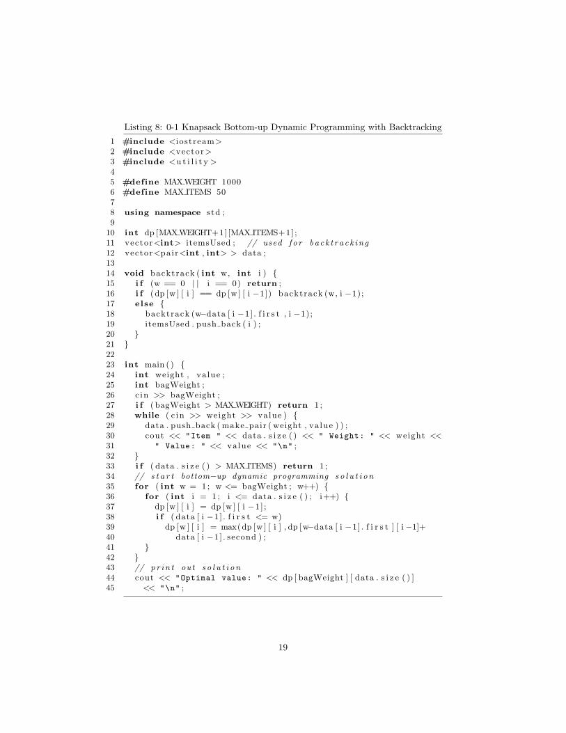
Listing 8: 0-1 Knapsack Bottom-up Dynamic Programming with Backtracking1 #include <iostream>2 #include <vector>3 #include <u t i l i t y >45 #define MAXWEIGHT 10006 #define MAX ITEMS 5078 using namespace std ;9

10 int dp [MAXWEIGHT+1] [MAX ITEMS+1] ;11 vector<int> itemsUsed ; // used f o r back t r a c k ing12 vector<pair<int , int> > data ;1314 void backtrack ( int w, int i ) {15 i f (w == 0 | | i == 0) return ;16 i f (dp [w ] [ i ] == dp [w ] [ i −1]) backtrack (w, i −1);17 else {18 backtrack (w−data [ i −1] . f i r s t , i −1);19 itemsUsed . push back ( i ) ;20 }21 }2223 int main ( ) {24 int weight , va lue ;25 int bagWeight ;26 c in >> bagWeight ;27 i f ( bagWeight > MAXWEIGHT) return 1 ;28 while ( c in >> weight >> value ) {29 data . push back ( make pair ( weight , va lue ) ) ;30 cout << "Item " << data . s i z e ( ) << " Weight: " << weight <<31 " Value: " << value << "\n" ;32 }33 i f ( data . s i z e ( ) > MAX ITEMS) return 1 ;34 // s t a r t bottom−up dynamic programming s o l u t i o n35 for ( int w = 1 ; w <= bagWeight ; w++) {36 for ( int i = 1 ; i <= data . s i z e ( ) ; i++) {37 dp [w ] [ i ] = dp [w ] [ i −1] ;38 i f ( data [ i −1] . f i r s t <= w)39 dp [w ] [ i ] = max(dp [w ] [ i ] , dp [w−data [ i −1] . f i r s t ] [ i−1]+40 data [ i −1] . second ) ;41 }42 }43 // p r i n t out s o l u t i o n44 cout << "Optimal value: " << dp [ bagWeight ] [ data . s i z e ( ) ]45 << "\n" ;

19

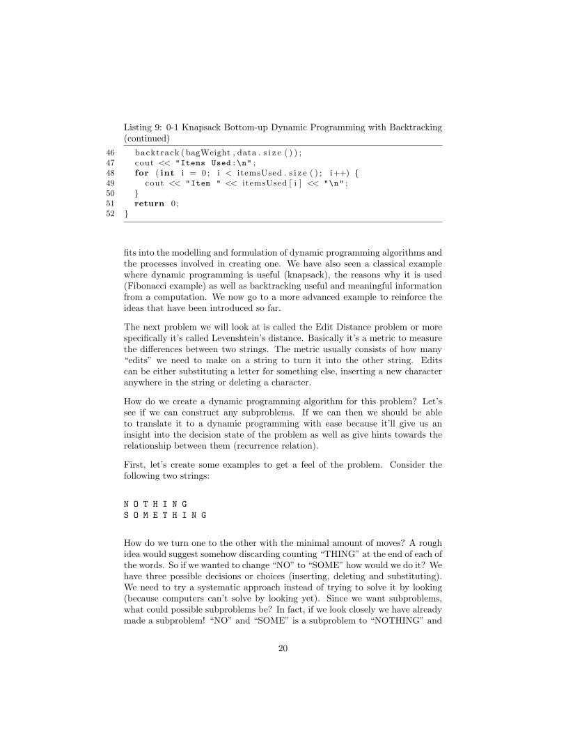
Listing 9: 0-1 Knapsack Bottom-up Dynamic Programming with Backtracking(continued)

46 backtrack ( bagWeight , data . s i z e ( ) ) ;47 cout << "Items Used:\n" ;48 for ( int i = 0 ; i < itemsUsed . s i z e ( ) ; i++) {49 cout << "Item " << itemsUsed [ i ] << "\n" ;50 }51 return 0 ;52 }

fits into the modelling and formulation of dynamic programming algorithms andthe processes involved in creating one. We have also seen a classical examplewhere dynamic programming is useful (knapsack), the reasons why it is used(Fibonacci example) as well as backtracking useful and meaningful informationfrom a computation. We now go to a more advanced example to reinforce theideas that have been introduced so far.

The next problem we will look at is called the Edit Distance problem or morespecifically it’s called Levenshtein’s distance. Basically it’s a metric to measurethe differences between two strings. The metric usually consists of how many“edits” we need to make on a string to turn it into the other string. Editscan be either substituting a letter for something else, inserting a new characteranywhere in the string or deleting a character.

How do we create a dynamic programming algorithm for this problem? Let’ssee if we can construct any subproblems. If we can then we should be ableto translate it to a dynamic programming with ease because it’ll give us aninsight into the decision state of the problem as well as give hints towards therelationship between them (recurrence relation).

First, let’s create some examples to get a feel of the problem. Consider thefollowing two strings:

N O T H I N GS O M E T H I N G

How do we turn one to the other with the minimal amount of moves? A roughidea would suggest somehow discarding counting “THING” at the end of each ofthe words. So if we wanted to change “NO” to “SOME” how would we do it? Wehave three possible decisions or choices (inserting, deleting and substituting).We need to try a systematic approach instead of trying to solve it by looking(because computers can’t solve by looking yet). Since we want subproblems,what could possible subproblems be? In fact, if we look closely we have alreadymade a subproblem! “NO” and “SOME” is a subproblem to “NOTHING” and

20

“SOMETHING”. How did we get there? We looked at the ends and decidedthat since they were equal, we skipped them. This is a sufficient and goodstarting point. Let’s try making the state being the last characters of the firstand second string we are looking at. For example at the start we let x = 6 andy = 8 (assuming 0-based index), the last characters of their respective strings.Now we compare the characters current in position x and y. If they are equal,we will do what we did implicitly, skip them. So what happens on x = 1 andy = 3 (“O” and “E”)? Well we have multiple choices:

1. We use substitution; this will make O become E. This will incur a costof 1. Now the subproblems for this decision would be x = 0 and y = 2because we made them the same.

2. We use deletion; we can delete O and hope to find a better match fromstring 1 later on. This will incur a cost of 1. Now the subproblems for thisdecision would be x = 0 and y = 3 because we “ignore” the O because wedeleted it, however we still need to match it to E because we didn’t deletethat.

3. We use insertion; we insert E after O, so there will be a new match. Thesecond string will decrease by 1 position because the E was matched bythe insertion. However, the first string stays in the same position becausewe still need to do something with the O, we merely “put it off” by doingan insertion. So the new subproblem for this decision would be x = 1 andy = 2.

Those were our three choices; in fact, they make perfect subproblems becausefirstly, it’s systematic and easily implementable. Second, it considers all possi-ble cases where we can modify the string. Third, subproblems depend only onstrictly smaller parts of the string and no overlapping occurs, so the order/de-pendencies can be implemented correctly. So now we have decided our state tobe the two positions relative to the positions we are up to in the two strings.Our recurrence relation can be deduced directly from the three cases:

F (x, y) = min

F (x− 1, y) + 1F (x, y − 1) + 1F (x− 1, y − 1) + d(x, y)

F (x, y) = 0 if x < 0 or y < 0

d(x, y) ={

0 if a[x] = b[y]1 otherwise

Note that d(x, y) evaultes to a cost of 1 if the characters in the current stringpositions don’t match, otherwise d(x, y) evaluates to a cost of 0 (because there

21

is no need to substitute since they have matching characters). Once our recur-rence relation is defined we can implement it. Here we will demonstrate bothtop-down and bottom-up implementations – it’s also a good time to practiceimplementation skills, so it’s a good idea to try and implement your own codebased on the above recurrence before looking at the supplied source code.

See Listing 10 for a memoization approach to the Edit Distance problem. SeeListing 11 for a bottom-up dynamic programming approach to the Edit Distanceproblem.

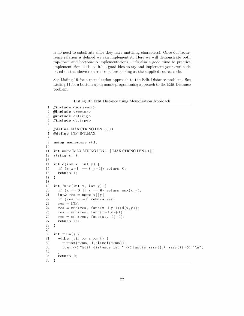
Listing 10: Edit Distance using Memoization Approach1 #include <iostream>2 #include <vector>3 #include <s t r i ng >4 #include <cctype>56 #define MAX STRING LEN 50007 #define INF INT MAX89 using namespace std ;

1011 int memo[MAX STRING LEN+1] [MAX STRING LEN+1] ;12 s t r i n g s , t ;1314 int d( int x , int y ) {15 i f ( s [ x−1] == t [ y−1]) return 0 ;16 return 1 ;17 }1819 int func ( int x , int y ) {20 i f ( x == 0 | | y == 0) return max(x , y ) ;21 int& re s = memo[ x ] [ y ] ;22 i f ( r e s != −1) return r e s ;23 r e s = INF ;24 r e s = min ( res , func (x−1,y−1)+d(x , y ) ) ;25 r e s = min ( res , func (x−1,y )+1);26 r e s = min ( res , func (x , y−1)+1);27 return r e s ;28 }2930 int main ( ) {31 while ( c in >> s >> t ) {32 memset (memo,−1 , s izeof (memo) ) ;33 cout << "Edit distance is: " << func ( s . s i z e ( ) , t . s i z e ( ) ) << "\n" ;34 }35 return 0 ;36 }

22

Listing 11: Edit Distance using Bottom-up Dynamic Programming1 #include <iostream>2 #include <s t r i ng >34 #define MAX STRING LEN 500056 using namespace std ;78 int dp [MAX STRING LEN+1] [MAX STRING LEN+1] ;9 s t r i n g s , t ;

1011 int d( int x , int y ) {12 i f ( s [ x−1] == t [ y−1]) return 0 ;13 return 1 ;14 }1516 int main ( ) {17 while ( c in >> s >> t ) {18 memset (dp , 0 , s izeof (dp ) ) ;19 for ( int i = 0 ; i <= s . s i z e ( ) ; i++) dp [ i ] [ 0 ] = i ;20 for ( int j = 0 ; j <= t . s i z e ( ) ; j++) dp [ 0 ] [ j ] = j ;21 for ( int i = 1 ; i <= s . s i z e ( ) ; i++) {22 for ( int j = 1 ; j <= t . s i z e ( ) ; j++) {23 dp [ i ] [ j ] = min (dp [ i −1] [ j ]+1 ,min (dp [ i ] [ j −1]+1,24 dp [ i −1] [ j−1]+d( i , j ) ) ) ;25 }26 }27 cout << "Edit Distance is: " << dp [ s . s i z e ( ) ] [ t . s i z e ( ) ]28 << "\n" ;29 }30 return 0 ;31 }

4.2 Performance Differences

We will now discuss the performance differences between the two approaches –should you opt for one over the other? Are there any rough indicators to suggestwhen one should be used over the other?

We will now to a mini-benchmark on the two approaches. After writing arandom string generator that generates two strings based on a specified length– we feed a collection of such strings into our program (i.e. by piping). Afterdoing a small test of roughly 20 random strings of possible size up to 1000length, we have the following numbers:

Memoization Approach: 1.683s

23

Dynamic Programming Approach: 1.094s

Most of the execution time was actually due to the allocation of the largecaching/dynamic programming array. If we modified our source code to al-locate 1001x1001 sized arrays rather than 5001x5001 arrays the execution timesgets cut to:

Memoization Approach: 0.941sDynamic Programming Approach: 0.488s

So certainly it seems the bottom-up approach runs more efficiently than thememoization approach in this test. For further tests, we bumped up the maxi-mum string length to 5000. We roughly collected around 30 of such strings andthe same strings on our two different programs. Here, the algorithm runs muchslower than it did previously:

Memoization Approach: 44.563sDynamic Programming Approach: 14.295s

Here we can see that the bottom-up approach becomes more efficient as theinput size grows. Why? This is due to the overhead for recursive calls for thememoization approach, it really magnifies as you have larger inputs because ittakes a longer time before the caching mechanism kicks in for repeated calls. Infact, it becomes rather dangerous to use memoization due to the risk of stackoverflow from a deep recursive tree. So you should definitely opt to use bottom-up dynamic programming if you can, but it generally isn’t as large of an issueas it seems to be.

Chances are, if the time required grows exponentially then either of the ap-proaches would be too slow to work in practice for even modest sized inputs.For strict time limits (such as algorithmic competitions) there may be caseswhere the bottom-up approach will pass within the time limit whilst the mem-oization approach won’t. A general indicator to use a bottom-up approach iswhen the recursive tree becomes too deep. This can be due to the fact that fur-ther subproblems only reduce the parameters by a small amount (in this caseby 1, since f(W, I) calls f(W − 1, I − 1), f(W − 1, I), f(W, I − 1)). So therecursive tree doesn’t “back out” for a long while – you can think of this as along depth first search tree (DFS has the same problem as memoization), henceit results in a deep recursive tree.

So when should you use memoization over the bottom-up approach? These usu-ally occur when only a minority of the subproblems of a problem is important.Since the bottom-up approach calculates all subproblems up to the parametersof a problem whether it is needed or not, this can result in many unnecessary

24

calculations. Here, memoization shines because it only calls the subproblemsthat it needs from the recurrence relation. Calculating binomial coefficients

(nk

)is a good example. If we tried to calculate

(1000

4

), then the classical bottom-up

approach would need to calculate all of Pascal’s triangle up to the row 1000(including all unnecessary columns). In this case, the number of calculationsrequired for the bottom-up approach would always be: n(n − 1)/2 (arithmeticseries), whereas the number of calculations required by the memoization wouldbe much less than this (the number of calculations required are actually vari-able, it would require more as the k becomes closer to n/2 but even still, itwould be less than the bottom-up approach).

5 Overview

We have looked at a range of issues involving the modelling, implementationand properties of dynamic programming algorithms through the use of classicalexamples. This tutorial should equip you with a better sense on how dynamicprogramming algorithms works as well as a general idea on how to solve one.As with most things in life, only practice can help you fully understand thispowerful and general algorithmic tool. There will be a further tutorial basedon “non-classical” algorithms that tackles more challenging problems than theones seen in this tutorial so far, it will also introduce some neat implementationtricks that you will find useful.

6 Problems

Practice what was discussed in this tutorial with a set of elementary and clas-sical dynamic programming problems! Note: These are roughly in the order ofdifficulty. These problems have no strict input structure, choose one that youlike and stick with it.

6.1 Problem 1: Longest Increasing Subsequence

Difficulty: EasyJohn likes to play with numbered blocks everyday, what he is particularly inter-ested in is finding increasing subsequences of the blocks. In particular, he wouldlike to know the longest length of such increasing subsequences – preferably withan example to re-create such a subsequence. A subsequence isn’t necessarily con-tiguous, for example, today John found that his numbered blocks were in thefollowing order: 3, 2, 9, 5, 6, 8.

An example of an increasing subsequence is 5, 6, 8 or 2, 5 (note that the 2 and

25

5 are not contiguous in the sequence). In this example, John helps you andpoints out that the length of the longest increasing subsequence is actually oflength 4: 2, 5, 6, 8 or 3, 5, 6, 8. Unfortunately as smart as John is, his havingtrouble working out the longest increasing subsequence for a large sequence (upto a sequence length of 10,000). Help him out by writing a program that printsout the length of the longest increasing subsequence, you must also print outa subsequence that corresponds to this length (by using backtracking or othermeans).

Possible file/input structure:

Line 1: Length of Sequence (n)Line 2: Followed by n integers

Example of such a structure (from John’s example):

63 2 9 5 6 8

Example output:

Length: 4Subsequence: 2 5 6 8

Hint: The intended complexity is O(n2) time. It can actually be solved inO(n log(n)) time but this is more complex than the idea required here. Thetime complexity gives a hint on the structure of the program (think of the forloops!).

Bigger Hint: A possible state for the problem is F (S) = the longest increasingsubsequence with the last element to be index S.

Even Bigger Hint: Recurrence relation is:

F (S) = max{F (S), F (n) + 1}, if A[n] < A[S] where n < S

6.2 Problem 2: Binomial Coefficients

Difficulty: EasyJohn likes to count things, unfortunately for him – he doesn’t know how tocount the number of ways to choose k items from a set of n items. Write aprogram that does this for him given input n and k.

26

Background: This is simply a basic mathematical problem relating to binomialcoefficients. Define

(nk

)as the number of ways to choose k items from a set of

n items. Then we can define a recurrence relation based on the combinatorialargument: you can either choose item k in which there will be n − 1 itemsremaining with k − 1 more to choose, or you can not choose item k in whichthere will be n−1 items remaining with k more to choose. Now we can producea recurrence relation:

(n

k

)=(

n− 1k

)+(

n− 1k − 1

)Hint: Part of the recurrence relation is defined for you, the only thing left isto determine the base cases and simply implement it! For our purposes,

(n0

)will always equal 1, because there is one way to choose nothing: don’t chooseanything.

Bigger Hint: Base cases to be determined:(nn

),(n0

). Optional base case:

(n1

).

Even Bigger Hint:(nn

)= 1,

(n1

)= n,

(n0

)= 1.

6.3 Problem 3: Longest Common Subsequence

Difficulty: Easy-Medium

John has recently became interested in subsequences, as evidently in Problem1. Since you have solved that problem for him, John now gives you a harderproblem that he needs help with. He has two character strings, and wishes toknow the length of the longest common subsequence of the two strings. Likein Problem 1, a subsequence isn’t necessarily contiguous. John gives you aninstance of the problem he has solved, the two strings are “DYNAMIC” and“PROGRAMMING”. He states that the longest common subsequence is 3: ’A’,’M’, ’I’. Not convinced, you ask him to give you another example. He gives youanother: “CLASSICAL” and “CAPITAL”, the longest being 5: ’C’, ’A’, ’I’, ’A’,’L’. Now, it’s your turn to write a program that solves the problem, given twostrings – find the longest common subsequence. Optionally, to impress Johneven more – also print out an example of such a subsequence (i.e. “AMI” and“CAIAL” in the two examples).

Hint: This is similar to the Edit Distance problem, start from the back andwork towards the front.

Bigger Hint: This is a 2-D Dynamic Programming problem (i.e. 2D caching/DParray).

Even Bigger Hint: The state is: F (X, Y ) = the length of the longest common

27

subsequence using string 1 from index 0 to X and string 2 from index 0 to Y.Think of how the Edit Distance problem works, when two characters matchwe added 0, but in this case we want it to add 1 to the length (since we arelooking for common elements). If two characters don’t match, we recursivelycheck subproblems by deletion/inserting, here we want the maximum of thesesubproblems. Try and formulate the recurrence relation now.

6.4 Problem 4: Handshaking Problem

Difficulty: Medium

John has recently joined a secret cult of, handshakers! In a cult meeting, eachmember is required to shake hands with exactly one other cult member in acircular table. All handshakes happen at the same time because it would taketoo long to do so otherwise. John has finished the meeting and has returnedhome safely, now he wonders how many ways were there of shaking hands if nohandshake can cross another. There were no clones, so each person is differentand distinguishable, so you can rotate a shaking configuration to yield a differentshake. Given the number of cult members there were (n), write a program thatreturns the number of handshake configurations that could of taken place in themeeting. You may assume there are an even number of cult members (otherwisethere would be a loner).

Some examples:

• For 2 Cult Members (John and the cult leader), there is only 1 shakeconfiguration – John just shakes the Cult Leader’s hand.

• For 4 Cult Members, there are three possible shaking configurations, only2 of them are valid. Hence there are two ways to shake. The diagrambelow shows this, only the first two are valid because the third one requireshandshakes to cross which is invalid.

• The next day, John asked the cult leader for hints (the Cult Leader isreally good with numbers). The cult leader replied “For 50 cult members,there are 4861946401452 possible shaking configurations!”.

Hint: Draw diagrams and try and visualise the problem before doing anythingelse!

Bigger Hint: This is actually a case of Catalan Numbers, however – you don’tneed to know this to solve it. If your stuck, you can just read about Catalannumbers and see how it relates here. As a consequence, the Catalan numbersrecurrence is the same as what we need for this problem.

28

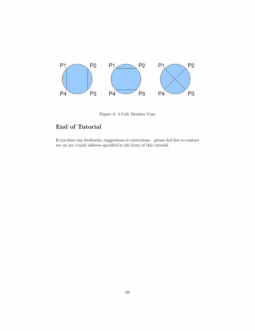
Figure 3: 4 Cult Member Case

End of Tutorial

If you have any feedbacks, suggestions or corrections – please feel free to contactme on my e-mail address specified in the front of this tutorial.

29