Downscaling daily precipitation over the Yellow River source region in China: a comparison of three statistical downscaling methods

1

This is the final accepted version. The published version is available through http://link.springer.com/article/10.1007/s00704-012-0745-4

Citation: Hu, Y., Maskey, S. and Uhlenbrook, S. (2013). Downscaling daily precipitation over the Yellow River source region in China: A comparison of three statistical downscaling methods. Theoretical and Applied Climatology, 112: 447-460.

1

Downscaling daily precipitation over the Yellow River source region in 2 China: A comparison of three statistical downscaling methods 3

4 Yurong Hu1, 2 *, Shreedhar Maskey2, Stefan Uhlenbrook2, 3 5

1 Yellow River Conservancy Commission, Zhengzhou 450003, People’s Republic of 6 China 7 2 UNESCO-IHE Institute for Water Education, PO Box 3015, 2601 DA Delft, The 8 Netherlands 9 3 Delft University of Technology, Department of Water Resources, PO Box 5048, 2600 10 GA Delft, The Netherlands 11 * Corresponding author: E-mail: [email protected]; Tel: +86-371-66020946; Fax: 12 +86-371-66020737. 13

14 Abstract: Three statistical downscaling methods are compared with regard to their ability 15 to downscale summer (June-September) daily precipitation at a network of 14 stations 16 over the Yellow River source region from the NCEP/NCAR reanalysis data with the aim 17 of constructing high-resolution regional precipitation scenarios for impact studies. The 18 methods used are the Statistical Downscaling Model (SDSM), the Generalized LInear 19 Model for daily CLIMate (GLIMCLIM), and the non-homogeneous Hidden Markov 20 Model (NHMM). The methods are compared in terms of several statistics including 21 spatial dependence, wet- and dry-spell length distributions and inter-annual variability. In 22 comparison with other two models, NHMM shows better performance in reproducing the 23 spatial correlation structure, interannual variability and magnitude of the observed 24 precipitation. However, it shows difficulty in reproducing observed wet- and dry-spell 25 length distributions at some stations. SDSM and GLIMCLIM showed better performance 26 in reproducing the temporal dependence than NHMM. These models are also applied to 27 derive future scenarios for six precipitation indices for the period 2046-2065 using the 28 predictors from two GCMs (CGCM3 and ECHAM5) under the IPCC SRES A2, A1B and 29 B1scenarios. There is a strong consensus among two GCMs, three downscaling methods 30 and three emission scenarios in the precipitation change signal. Under the future climate 31 scenarios considered, all parts of the study region would experience increases in rainfall 32 totals and extremes that are statistically significant at most stations. The magnitude of the 33 projected changes is more intense for the SDSM than for other two models, which 34 indicates that climate projection based on results from only one downscaling method 35 should be interpreted with caution. The increase in the magnitude of rainfall totals and 36 extremes is also accompanied by an increase in their inter-annual variability. 37 38

2

1 Introduction 1 It is expected that global climate change will have a strong impact on water resources in 2 many regions of the world (Bates et al. 2008). As a key component of the hydrological 3 cycle, modeling these impacts requires high-resolution regional precipitation scenarios as 4 input to impact models. Currently global climate models (GCMs) are the most 5 appropriate tools for modeling future global scale climate change. Although the 6 usefulness of these models is unquestionable, they provide information at a resolution 7 that is too coarse to be directly used in impact studies (Xu 1999). GCMs are also limited 8 in skill to represent subgrid-scale features and dynamics such as convection and 9 topography (Xu 1999), which are of importance for impact studies on a catchment scale. 10 These limitations become more problematic when a study focuses on precipitation, which 11 strongly depends on subgrid-scale processes (Wilby and Wigley 2000) and on regions 12 with complex and sharp orography (Schmidli et al. 2006). Consequently, downscaling 13 techniques have been developed to bridge the gap between what GCMs are able to 14 simulate well and what is needed for the catchment scale climate change impact research. 15 Among the different downscaling approaches, statistical downscaling is the most widely 16 used one to construct climate change information at a station or local scales because of 17 their relative simplicity and less intensive computation. Statistical downscaling methods 18 are generally classified into three groups (Wilby and Wigley 1997): regression models, 19 weather typing schemes and weather generators. Weather generators are adapted for 20 statistical downscaling by conditioning their parameters on large-scale atmospheric 21 predictors (Maraun et al. 2010). They are often used in combination with either 22 regression methods or weather typing schemes. Statistical models can also be divided 23 into single and multi-site methods. The single-site methods model each station 24 independently. The multi-site methods model all sites simultaneously, thereby 25 maintaining inter-station relationships, e.g. spatial correlation, which is one of the 26 important considerations for climate change impact studies over large river basins. 27

Although there is a large body of literature where an intercomparison of different 28 downscaling methods has been made (e.g. Wilby et al. 1998; Mehrotra et al. 2004; Diaz-29 Nieto and Wilby 2005; Frost et al. 2010; Liu et al. 2011; Liu et al. 2012), very few of 30 these studies have dealt with downscaling precipitation in remote mountainous areas. To 31 the best of our knowledge, no other studies have reported downscaling of precipitation in 32 the literature for this catchment with an exception of Xu et al. (2009), who investigated 33 the response of streamflow to climate change in the headwater catchment of the Yellow 34 River basin using the SDSM model (Wilby et al. 2002) and a perturbation based 35 technique called the 'delta-change' method (Prudhomme et al. 2002). The SDSM is a 36 single site downscaling method. The delta-change method involves adjusting the 37 observed time series by adding the differences (for temperature) or multiplying the ratio 38 (for precipitation) between future and present climates simulated by the GCMs. 39

The need for regional precipitation scenarios for impact and hydrological studies is 40 particularly urgent for the Yellow River source region. First, located in mountainous 41 areas, this region is expected to be sensitive to global climate change since mountains in 42 many parts of the world (e.g. the Andes and the Himalayas) are very susceptible to a 43 changing climate in view of their complex orography and fragile ecosystem (Beniston 44 2003). Second, the Tibetan Plateau, where the study area is located, has been identified as 45 one of the most sensitive areas to global climate change due to its earlier and larger 46

3

warming trend in comparison to the Northern Hemisphere and the same latitudinal zone 1 in the same period (Liu and Chen 2000). As a consequence, it can be expected that the 2 Yellow River source region might be particularly susceptible to global climate change. 3 This in turn might have considerable impacts on water availability in the entire Yellow 4 River basin as the source region contributes about 35% of the total annual runoff of the 5 entire Yellow River. It is therefore important to project future precipitation scenarios over 6 the region in order to provide useful information for impact studies and 7 adaptation/mitigation policy responses. This study is aimed at testing three different 8 statistical downscaling methods in their ability to reconstruct observed daily precipitation 9 over the Yellow River source region and applying them to develop future precipitation 10 scenarios for the region. The three statistical downscaling methods used in this study are: 11 the Statistical DownScaling Model (SDSM) (Wilby et al. 2002), the Generalized LInear 12 Model for daily CLIMate (GLIMCLIM) (Chandler 2002), and the non-homogeneous 13 Hidden Markov Model (NHMM) (Hughes and Guttorp 1994). All three models have 14 been tested in a range of geographical contexts (Wetterhall et al. 2006; Tryhorn and 15 DeGaetano 2010; Chandler 2002; Chandler and Wheater 2002; Yang et al. 2005; Fealy 16 and Sweeney 2007; Hughes et al. 1999; Mehrotra et al. 2004; Kioutsioukis et al. 2008). 17 Several previous studies have also compared some of these downscaling models in 18 different river basins (Liu et al. 2011; Frost et al. 2011; Liu et al. 2012). However, all of 19 the previous comparisons were limited to the present climate and the projections for the 20 future climate were not included in their study. 21

2 Study area and data set 22

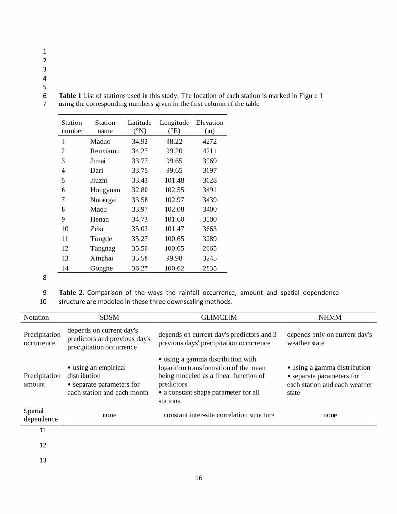
2.1 Study area 23 The study region is located in the northeast Qinghai-Tibetan Plateau, spanning between 24 95º50´45''E-103º28´11''E and 32º12'11''N-35º48'7''N (Fig. 1). It covers an area of 121,972 25 km2 (15% of the whole Yellow River basin), characterized by highly variable 26 topographic structure ranging from 6282 m a.s.l. in the Anyemqen Mountains in the west 27 to 2546 m a.s.l. in the village of Tangnag in the east, which strongly influences the local 28 climate variables and their spatial variability. The study area has a cold, semi-humid 29 climate, characterized by the typical Qinghai-Tibetan Plateau climate system. The 30 precipitation pattern in this region is strongly governed by the southwest Asian monsoon, 31 which brings moist, warm air in summer and dry, cool air during winter. In winter, it has 32 the characteristics of typical continental climate, which is controlled by the high pressure 33 of the Qinghai–Tibetan Plateau lasting for about 7 months. During summer it is affected 34 by southwest monsoon, producing heat low pressure with abundant water vapor and a lot 35 of rainfall and thus forms the Plateau sub-tropical humid monsoon climate. Annual 36 average daily temperature varies between -4 ºC and 2 ºC from the southeast to the 37 northeast. July is the warmest month, with a mean daily temperature of 8 ºC. From 38 October to April the temperature remains well below 0 ºC. Mean annual precipitation 39 ranges from 800 mm/a in the southeast to 200 mm/a in the northwest. Up to 75-90% of 40 the total annual precipitation falls in the summer season (June to September) caused by 41 the southwestward water vapor from the Bay of Bengal in the Indian Ocean. In the 42 months from November to March, more than 78% of the total precipitation falls in the 43 form of snow. However, the total amount of annual snowfall accounts for less than 10% 44 of the annual precipitation. 45

4

2.2 Data set 1

2.2.1 Observed station data 2 The observed daily precipitation data used in this study are for the period 1961-1990 3 from 14 stations distributed throughout the study region. Fig. 1 depicts the geographical 4 location of the stations in the study region and Table 1 shows their latitude, longitude and 5 altitude. The homogeneity of the data was tested by applying the double mass curve 6 method on a monthly basis for each station (Hu et al. 2011). Slightly less than 0.03% of 7 the data from two stations were missing, which were infilled using the records from 8 neighboring stations. We only focus on downscaling summer (monsoon) precipitation 9 because there is negligible rainfall during the remaining part of the year. A threshold of 1 10 mm/d is used to discriminate between wet and dry days. 11 2.2.2 Reanalysis data 12 In addition to the observed data, large-scale atmospheric variables derived from the 13 National Center for Environmental Prediction /National Centre for Atmospheric Research 14 (NCEP/NCAR) reanalysis data set (Kalnay et al., 1996) on a 2.5° × 2.5° grid over the 15 same time period as the observation data were employed for model calibration and 16 validation. These variables include specific humidity, air temperature, zonal and 17 meridional wind speeds at various pressure levels and mean sea level pressure. The 18 predictor domain extends from 30°N to 40°N and from 92.5°E to 107.5°E covering the 19 entire study region (Fig. 1). 20 2.2.3 GCM data 21 In order to project future precipitation scenarios, output from two GCMs under the 22 Intergovernmental Panel on Climate Change Special Report on Emissions Scenarios 23 (IPCC-SRES) A2, A1B and B1 were used: (1) the Canadian Center for Climate 24 Modelling and Analysis (CCCma) 3nd Generation (CGCM3.1 (T47)), and (2) the 25 ECHAM5/MPI-OM GCM from the Max-Planck-Institute for Meteorology, Germany 26 (hereafter ECHAM5). Both models are coupled atmosphere-ocean models. CGCM3 has a 27 horizontal resolution of T47 (approximately 3.75° latitude × 3.75° longitude) and 32 28 vertical levels. ECHAM5 has a horizontal resolution of T63 (approximately 1.875° 29 latitude × 1.875° longitude) and 31 vertical levels. These GCM data are obtained from 30 the Program for Climate Model Diagnosis and Intercomparison (PCMDI) website 31 (http://www-pcmdi.iinl.gov). The A2, A1B and B1 scenarios span almost the entire IPCC 32 scenario range, with the B1 being close to the low end of the range, the A2 to the high 33 end of the range and A1B to the middle of the range. The GCM simulations 34 corresponding to the present (1961-1990) and future climate (2046-2065) were 35 considered in the analysis. Prior to use in this study, both GCMs grids were linearly 36 interpolated to the same 2.5°× 2.5° grids fitting the NCEP reanalysis data. 37

3 Methodology 38

3.1 Precipitation indices 39 Six precipitation indices were selected in order to examine and simulate the changes of 40 the mean and extreme conditions over the study region under future emission scenarios. 41

a) prcptot – total precipitation [mm]; 42

b) pq95 – 95th percentile of precipitation on days with precipitation >1mm [mm/d]; 43

5

c) pq95tot – total precipitation falling in days with amounts > the corresponding 1 long-term 95th percentile (calculated only for wet days and for the baseline period 2 1961-1990) [mm]. 3

d) pfl95 – fraction of total precipitation from events > long-term 95th percentile of 4 precipitation [mm/mm]. 5

e) px5d – maximum total precipitation from any consecutive 5 days [mm]. 6

f) pxcdd – maximum number of consecutive days with precipitation < 1 mm [d]. 7

3.2 Choice of predictors 8 There is small agreement on the most appropriate choice of predictor variables. The 9 choice of predictors depends on the region, the characteristics of the large-scale 10 atmospheric circulation, seasonality, the topographic context, and the predictand to be 11 downscaled (Anandhi et al. 2008). In this study the predictors were first selected taking 12 into consideration the monsoon rainfall generation mechanism. Monsoon rainfall in the 13 study region is caused by high temperature in the land area and subsequent generation of 14 low-pressure zone. This results in wind flow with moisture from the Bay of Bengal and 15 the western Pacific Ocean to the land area (Lan et al. 2010) while northwestern cold air 16 current plays a major role in monsoon rainfall generation. Based on this, a number of 17 atmospheric variables were taken as the potential predictors including air temperature, 18 specific humidity, zonal and meridional wind at various pressure levels and mean sea 19 level pressure. These potential predictors were then screened through a correlation 20 analysis with daily monsoon precipitation at each of the 14 stations. Furthermore, 21 experiences and recommendations from similar studies in China and neighboring regions 22 were also taken into account (Wetterhall et al, 2006; Tripathi et al. 2006; Anandhi et al. 23 2008; Liu et al. 2011; Liu et al. 2012). The final set of predictors for downscaling of 24 precipitation was selected as follows: specific humidity at 300 and 500 hPa level, zonal 25 wind at 200, 300 and 500 hPa level and meridional wind at 850 and 1000 hPa level. The 26 explanatory power of a given predictor will vary both spatially and temporally for a given 27 predictand. The use of predictors directly overlying the target grid box is likely to fail to 28 capture the strongest correlation (between predictor and predictand), as this domain may 29 be geographically smaller in extent than the circulation domains of the predictors (Wilby 30 and Wigley 2000). Selecting the spatial domain of the predictors is subjective to the 31 predictor, predictand, season and geographical location (Anandhi et al. 2009). On the 32 basis of these recommendations and monsoon rainfall generation mechanism, the spatial 33 domain of the predictors considered in this study was chosen as 35 grid points lying an 34 extended area covering the entire study region (Fig. 1). 35

The predictors were first standardized at each grid-point by subtracting the mean and 36 dividing by the standard deviation. A principal component analysis (PCA) was then 37 performed to reduce the dimensionality of the predictors. The first eight principal 38 components (PCs), which account for more than 90% of the total variance, were then 39 used as input to the downscaling model. The principal components were selected on the 40 basis of the percentage of variance of original data explained by individual principal 41 component. This criterion was also used by Tripathi et al. (2006), Anandhi et al. (2008), 42 Anandhi et al. (2009) and Ghosh (2010). Note that there are also other methods exist for 43

6

selecting the principal components, e.g. the elbow method used by Wetterhall et al. 1 (2006). 2

3.3 Statistical downscaling methods 3 The three downscaling models considered in this study all belong to stochastic 4 downscaling models. They mainly differ in the way their weather generator parameters 5 are conditioned on large-scale predictors or weather states. In SDSM the multiple linear 6 regression method is used to condition its weather generator parameters on large-scale 7 predictors, whereas in GLIMCLIM and NHMM this is done using a generalized linear 8 model and a weather state approach, respectively. In addition, SDSM is a single-site 9 model while GLIMCLIM and NHMM are multi-site models. Table 2 compares the ways 10 the rainfall occurrence, amount and spatial dependence structure are modeled in these 11 three downscaling methods. 12

3.3.1 SDSM 13 SDSM is described as a hybrid between a multivariate linear-regression method and a 14 stochastic weather generator. Large-scale predictors are used to linearly condition local-15 scale weather generator parameters (e.g. precipitation occurrence and intensity) at 16 individual stations. Precipitation is then modeled through a stochastic weather generator 17 conditioned on the predictor variables. The conditional probability of precipitation 18 occurrence on day t ( tω ) depends on the large-scale predictors and conditional 19

probability of the previous day’s precipitation occurrence ( 1tω − ) (Wilby et al. 2003). 20

Precipitation occurs if t trω > ( 0 1tr≤ ≤ ) where tr is a uniformly distributed random 21 number. The precipitation amount is modeled through an empirical distribution 22 conditioned on the predictors. For a full description, see Wibly et al. (2003). 23

The SDSM was applied with a common set of predictors to all the stations instead of 24 different sets of predictors for different stations in order to be consistent with the two 25 multi-site models (NHMM and GLIMCLIM). Precipitation was modeled as a conditional 26 process in which local precipitation amounts are correlated with the occurrence of wet-27 days, which in turn correlated with large-scale atmospheric predictors. A transformation 28 of the fourth root was applied to account for the skewed nature of the precipitation 29 distribution. In SDSM, it is possible to adjust the bias correction and variance inflation 30 parameters to overcome the problem of over- or under-estimation of the mean and 31 variance of downscaled variables. However, von Storch (1999) indicated that the 32 variance inflation approach adopted in SDSM is not meaningful because it fails to 33 acknowledge that local-scale variation is not completely explained by predictors. In this 34 study, SDSM was run with different adjustments made to the bias correction and variance 35 inflation to test the effect of altering these parameters on downscaled precipitation. 36 However, the alternation of the bias correction and variance inflation did not significantly 37 improve the downscaled results. Therefore, it was decided to use the default value for the 38 variance inflation and no bias correction. 39

3.3.2. GLIMCLIM 40 Similar to SDSM, GLIMCLIM also employs a regression based approach for specifying 41 weather generator parameters conditioned on the large-scale predictors. But it uses 42 logistic regression to model the rainfall probability and a gamma distribution to model 43

7

rainfall amounts. The logarithm of the mean precipitation amount is modeled as a linear 1 function of a set of predictors. The shape parameter of the gamma distribution is assumed 2 constant for all observations. The reader is referred to Chandler and Wheater (2002) and 3 Yang et al. (2005) for further details. 4

In GLIMCLIM, precipitation occurrence and amounts can be modeled with different 5 set of predictors. However, in order to be consistent with SDSM and NHMM a same set 6 of predictors were used to fit the occurrence and amounts model in GLIMCLIM 7 individually. Besides large-scale predictors, other covariates representing spatial 8 dependence, seasonality, autocorrelation and interaction terms can also be used. In this 9 study, site altitudes and the Legendre polynomial transformation of the site eastings and 10 northings are used to accommodate the non-homogeneity displayed across a region that 11 are not explained by the input predictors. The seasonality is represented using sine and 12 cosine components and the autocorrelation is modeled using the three previous days' 13 rainfall. By defining suitable dependence structures between sites, GLIMCLIM can 14 downscale precipitation at multiple stations simultaneously. For the occurrence model, 15 we used a beta-binomial distribution (see Yang et al. (2005) for a mathematical 16 derivation). The distribution has two parameters representing the mean, which varies in 17 time and is estimated from the probabilities derived from the occurrence model, and the 18 shape, which is assumed constant for all days and is estimated using the method of 19 moments (Chandler and Wheater, 2002; Yang et al. 2005). A small value of the shape 20 parameter indicates strong inter-site dependence. For the amounts model we used the 21 inter-site constant correlation structure of the transformed rainfall values called the 22 Anscombe residuals (Yang et al. 2005). 23

3.3.3. NHMM 24 Unlike SDSM and GLIMCLIM in which the weather generator parameters are 25 conditional directly on the predictors, NHMM conditions the weather generator 26 parameters on weather states. As a weather state based downscaling model the NHMM 27 relates synoptic-scale atmospheric predictors through a finite number of 'hidden' (i.e. 28 unobserved) weather states to multi-site daily precipitation occurrences. The temporal 29 evolution of these daily states is modeled as a first-order Markov process with state to 30 state transition probabilities conditional on a set of synoptic-scale atmospheric predictors. 31 The most likely weather state sequence is obtained from a fitted NHMM using the Viterbi 32 algorithm to assign each day to its most probable state (Forney, 1978). Unlike other 33 weather state (type) based downscaling models, the weather states in the NHMM are 34 defined from daily rainfall observations at a network of sites rather than a priori (Hughes 35 et al. 1999). 36

The NHMM makes two assumptions (Hughes et al. 1999). The first assumption states 37 that the n site precipitation process pattern on day t (Rt) depends only on the weather state 38 of day t (St), and the second assumption states that the weather state on day t (St) depends 39 both on the weather state on the previous day (St-1) and the values of the atmospheric 40 variables (Xt) on day t. The two assumptions determine the temporal structure in the 41 precipitation process. The first assumption states that the precipitation process (Rt) is 42 conditionally independent given the weather state. In other words, all the temporal 43 persistence in the precipitation processes is captured by the persistence in the weather 44 state. 45

8

Daily precipitation amount at each station is modeled as a combination of a delta 1 function (dry days modelling) and a gamma function (wet days modellling). In this study 2 the NHMM computations are performed using the Multivariate Nonhomogeneous 3 Hidden Markov Model (MVNHMM) toolbox (Kirshner, 2005b). Further details on 4 NHMM can be found in Hughes and Guttorp (1994), Hughes et al. (1999) and Krishner 5 (2005a). 6

For the NHMM model, calibration is to choose the appropriate number of hidden 7 weather states using the Bayesian Information Criterion (BIC). This involves the 8 sequential fitting of several NHMMs with an increasing number of weather states until 9 the BIC reaches its minimum value. For this study, the appropriate number of hidden 10 weather states is four. 11

3.3 Performance criteria 12 The standard split-sampling technique of model calibration and validation was 13 implemented in this work. The model calibration was performed for the monsoon seasons 14 (June-September) over the period 1961-1980, while the period 1981-1990 was used for 15 validation. Both the GLIMCLIM and NHMM models are calibrated for the 14-station 16 network concurrently as opposed to the SDSM model, which is calibrated on a station by 17 station basis. 18

The performance of the three downscaling models is evaluated by several criteria 19 relevant to hydrological studies: (i) the spatial correlation structure in terms of Spearman 20 cross correlation in the daily rainfall amounts, (ii) the ability to reproduce inter-annual 21 variability in terms of Spearman rank correlation, (iii) the mean difference between the 22 observed and simulated data, and (iv) the temporal structure (characterized by wet- and 23 dry-spell length) 24

4 Results and discussion 25 The results presented in the following subsection are based on 100 realizations of 26 downscaled precipitation from each of the methods. We also tested the sensitivity of 27 using more number of realizations (e.g. 200, 300, 400 and 500) but found no significant 28 changes in the results. 29

4.1 Validation of the three statistical downscaling models (1981-1990) 30

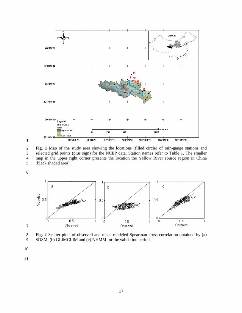
4.1.1 Spatial patterns 31 Accurate reproduction of the spatial pattern of the precipitation is essential for correct 32 simulation of river discharge over a large area. Fig. 2 present observed and modeled 33 Spearman cross correlation for daily precipitation amounts. As can be seen from the 34 figure, NHMM performed quite well in reproducing the spatial correlation for the 35 majority of station pairs. However, it underestimated the spatial correlations for highly 36 correlated stations. This indicates that although the hypothesis of conditional spatial 37 independence, given the weather state, captures much of the correlation between stations, 38 it is not sufficient to account for all the observed correlations between stations. The 39 unexplained local spatial correlation, which is induced by important subgrid-scale 40 features such as topography and convection, was not captured by this assumption. Similar 41 findings were reported by Bellone et al. (2000), Kioutsioukis et al. (2008) and Liu et al. 42 (2012). Both the SDSM and GLIMCLIM models show consistent under-estimation of the 43

9

spatial correlations for most station pairs (Fig. 2). The possible explanation for the poor 1 performance of SDSM and GLIMCLIM in representing the spatial dependence is that the 2 SDSM as a single-site model is trained on each station separately and therefore could not 3 effectively reproduce the inter-station correlations. GLIMCLIM, which was originally 4 designed for application over smaller areas with frontal (relatively homogeneous) 5 weather systems, models the spatial dependence by constraining it to be the same for all 6 site pairs involved. This is unrealistic in practice, particularly for large areas where inter-7 site dependence generally tends to be lower and vary with distance. Similar results were 8 obtained in other studies. Yang et al. (2005) discussed the difficulties of GLIMCLIM in 9 representing the spatial dependence over large areas. Frost et al. (2011) found that 10 GLIMCLIM tends to underestimate the spatial correlation with distance under Australian 11 condition. Liu et al. (2012) reported that GLIMCLIM markedly overestimated the spatial 12 correlation at longer distance under north China plain condition. The use of distance-13 dependent correlation structure in GLIMCLIM is worth investigating in the future. 14

4.1.2 Wet and dry spells 15 Figs. 3-4 compare the observed and modeled wet- and dry-spell length distributions at 16 three representative stations for the validation period. The results are in general similar 17 for the remaining stations. Overall, both SDSM and GLIMCLIM reproduce wet-spell 18 length distribution reasonably well, particularly for the short-duration spells less than 10 19 days, while it is found that wet-spell distribution at some stations is modeled less 20 accurately by NHMM in comparison to other two models. Clearly, this lower 21 performance of NHMM in representing wet-spell distributions may be attributed to its 22 assumption of conditional temporal independence of the precipitation process as 23 discussed in the description of the model in the method section. The difficulty in 24 reproducing the wet spell distribution by NHMM was also noted by Hughes and Guttorp 25 (1994) and was attributed to the assumption of conditional temporal independence of the 26 precipitation process in the NHMM. Liu et al. (2012) reported that NHMM performed 27 relatively poorer in reproducing the mean wet- and dry-spell length in comparison to 28 GLIMCLIM. As SDSM and GLIMCLIM model the temporal dependence of the 29 precipitation processes by assuming it to be conditionally Markov, i.e. the precipitation 30 process is conditional on the current day's atmospheric variables and the preceding days' 31 precipitation process (the previous day for SDSM and the three previous days for 32 GLIMCLIM), they are able to reproduce wet-spell length distribution reasonably well. In 33 comparison to wet spell, all the models show less skill in reproducing dry-spell length 34 duration. It should, however, be noted that these are not very frequent events in the 35 monsoon season. 36

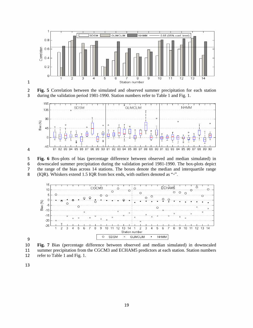
4.1.3 Interannual variability and the magnitude of observed summer precipitation 37 It is important for the downscaling models to be able to reproduce the interannual 38 variability reasonably well if they are to be used in climate change studies, otherwise, the 39 models lack in sensitivity to climate variability and their usefulness in climate change 40 studies can be questioned (Wetterhall et al. 2006). To estimate the interannual variability, 41 we calculate the Spearman rank correlation between the observed and median of 100 42 simulations at each station for the validation period (Fig. 5). The horizontal line in this 43 plot shows the value of the correlation coefficient above which they are statistically 44 significant at the 95% confidence level. Overall, NHMM performs relatively better than 45

10

other two models in reproducing the interannual monsoon precipitation variability. This 1 can be seen from the plot that NHMM exhibits relatively high correlation coefficients 2 which are statistically significant at the majority of the stations (9 out of 14 stations). 3 However, GLIMCLIM and SDSM perform less satisfactorily in reproducing interannual 4 monsoon precipitation variability with most stations (8 and 10 out of 14 stations, 5 respectively) having low and insignificant correlation coefficients. This could be due to 6 the reason that the two regression-based models are not able to capture some processes 7 (e.g. localized convection) that are driving interannual precipitation variability, because 8 only part of the local climate variability is related to large-scale climate variations. The 9 introduction of parametric inflation factor in the SDSM is found to be ineffective to 10 sufficiently represent variability in the downscaled precipitation (see von Storch (1999) 11 on the limitation of using inflation in downscaling to increase variance). However, 12 through a number of weather states defined from the 14-sation rainfall observations, 13 NHMM is able to capture local precipitation variability reasonably well. 14

Fig. 6 presents the percentage difference between the observed and median of 100 15 simulations at each station for each validation year. The whisker-box plots show the 16 biases across all stations. We can see that NHMM captures the magnitude of the observed 17 monsoon precipitation sufficiently well with much lower biases for almost the whole 18 validation period. However, the other two models perform less satisfactorily with an 19 overestimation at most stations for most of the validation period. 20

4.2 Downscaling precipitation for the present climate (1960-1990) 21

The downscaling models calibrated and validated using the NCEP predictors were driven 22 by the two GCMs predictors for the present climate (1961-1990) to evaluate whether 23 downscaled summer precipitation from the two GCMs can reproduce the variability of 24 the observed one. Fig. 7 presents the percentage difference between downscaled and 25 observed summer precipitation. The results show that the biases in the downscaled 26 summer precipitation are quite similar from GCM to GCM while they vary considerably 27 from downscaling model to downscaling model. The NHMM appears to be the best 28 performer when driven by both the CGCM3 and the ECHAM5 predictors with the biases 29 ranging from -2.5 to 1.3% across different stations. SDSM generally shows large positive 30 bias in the downscaled summer precipitation compared to those from the NHMM. The 31 GLIMCLIM shows mostly negative biases (underestimation), which are relatively larger 32 (-5 to -20%) than those of the other two models. 33

4.3 Downscaling precipitation for the future scenarios (2046-2065) 34

Three statistical models (calibrated) are used to downscale daily precipitation from two 35 GCMs for three emission scenarios. Estimated changes in the magnitude and the 36 distribution of six precipitation indices for a future period (2046-2065) are investigated 37 against the control period (1961-1990). The changes in the magnitude correspond to the 38 percentage difference between mean values of each index in the future period and those 39 in the control period. A two-tailed Student’s t-test for the 5% confidence level is 40 performed to check if the mean values from the present and future periods are 41 significantly different. 42

11

4.3.1 Estimated changes in the magnitude of precipitation indices 1

Fig. 8 depicts the changes in the magnitude of the six precipitation indices. We can see 2 that there is strong consistency in the climate change signals from different projections. 3 All of the projections suggest an increase in the indices related to the wet events (prcptot, 4 pq95, pq95tot, pfl95, px5d) and a decrease in the index related to the dry events (pxcdd). 5 The effect of the driving GCM on the magnitude of estimated changes is evident in Fig. 6 8, with CGCM3-driven projections showing relatively larger changes in the precipitation 7 indices than ECHAM5-driven ones. A comparison between the three downscaling 8 models shows that for all the indices considered SDSM predicts larger changes than 9 GLIMCLIM and NHMM. However, despite some notable differences in the results for 10 the control climate, it is interesting to note that the projected changes by GLIMCLIM and 11 NHMM are of similar magnitude. Compared to the differences due to the GCMs and 12 downscaling models, there are no clear systematic differences between the projected 13 changes for the three emission scenarios. The SDSM also shows large spatial variability 14 of the projected changes across stations, while the other two models show less spatial 15 variability, especially for the four wet extreme indices (pq95, pq95tot, pfl95, px5d). This 16 is probably due to the fact that SDSM is calibrated on individual station while other two 17 models are calibrated on multi-station basis. 18

Throughout the study region, all of the projections show statistically significant 19 increases in summer precipitation (prcptot) ranging from an average of 8 to 55%. Similar 20 results are obtained for the pq95tot index, but with much larger magnitude. On average, 21 pq95tot are expected to increase by 13 to 167%. As for the pq95 and the pfl95 indices, 22 the majority of the projections suggest a statistically significant increase at almost all 23 stations with the exception of the ECHAM5/GLIMCLIM-driven one in which most 24 stations reveal insignificant increases. Similar to the prcptot and the pq95tot indices, there 25 is also a pronounced increase in the consecutive 5-day precipitation total (px5d) over the 26 whole region with an average of 5 to 60%. In clear contrast to all the wet indices, the 27 maximum dry spell (pxcdd) is expected to decrease over the whole region, but most of 28 the decreases are statistically insignificant. 29

4.3.2 Changes in the distribution of precipitation indices 30

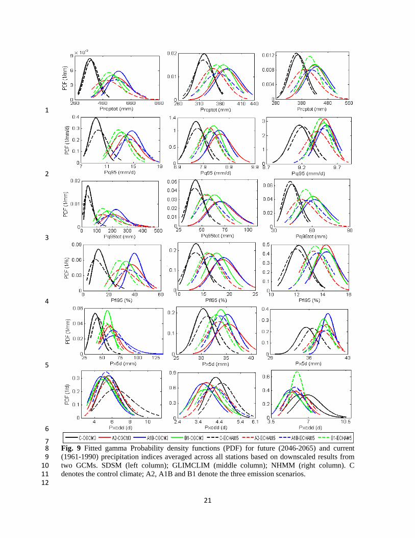
In this section, we analyzed changes in the distribution of the precipitation indices. Fig. 8 31 compares fitted gamma probability density functions (PDFs) of the precipitation indices 32 averaged across 14 stations for the control and future periods. Comparison of the scenario 33 and control PDFs reveals a substantial shift of the mean to the right of the distribution for 34 the wet indices and a small shift to the left for the dry index, suggesting a pronounced 35 increase in the precipitation indices related to the wet events and a small decrease in the 36 maximum dry spell. Concerning the shape of the distribution, it is noteworthy that the 37 scenario PDFs of the wet indices generally become wider and flatter in comparison to 38 that from the control period, which may suggest increased variability in future 39 precipitation. 40

The climate change signal derived from the present study implies a significant 41 increase in summer precipitation totals and extremes, and an insignificant decrease in the 42

12

maximum dry spell. This signal is in general agreement with previous modeling studies 1 over the neighboring areas, which may be interpreted as the warmer air in the future 2 climate being able to hold more moisture generated by increased evaporation from 3 warmer oceans. When this moister air moves over land, more intense precipitation is 4 produced (Meehl et al. 2005). Similar projections for 2081-2100 under the A1B scenario 5 were obtained for annual precipitation extremes over the headwater region of the Yangtze 6 River by Xu et al. (2009) based on statistical downscaling of six GCM outputs using the 7 SDSM model. Increases in extreme precipitation have also been found from the direct 8 GCM outputs over a large scale (Xu et al. 2011; Yang et al. 2012). Based on direct 9 outputs from three GCMs, Xu et al. (2011) suggested increases in the px5d and pfl95 10 indices and little change in the pxcdd during summer over the Huang-Huai-Hai River 11 Basins for 2011-2050 under the A1B scenario. Using the ensemble mean of five GCMs, 12 Yang et al. (2012) reported slight decreases in the pxcdd and general increases in the 13 px5d and pfl95 indices over most of the Tibetan Plateau by the end of the century under 14 the three scenarios (A2, A1B and B1). 15

5 Conclusions 16 Three statistical downscaling models have been compared in terms of their ability to 17 downscale summer (June-September) daily precipitation over the source region of the 18 Yellow River. These models were then applied to investigate possible changes in rainfall 19 totals and extremes by the middle of the 21st century using the predictors from two 20 GCMs (CGCM3 and ECHAM5) under the IPCC SRES A2, A1B and B1 scenarios. The 21 validation (1981-1990) results show that the NHMM model is generally better in 22 reproducing the spatial correlation structure, interannual variability and magnitude of 23 observed summer precipitation in comparison to other two models. The NHMM however 24 shows difficulty in reproducing the observed wet-and dry-spell length distribution. In 25 contrast, SDSM and GLIMCLIM show consistent underestimation of the spatial 26 correlations for most station pairs. This is due to the fact that the single-site model SDSM 27 was trained on each station separately, and the multi-site model GLIMCLIM simulates 28 the spatial rainfall dependence structure by constraining it to be the same for all site pairs 29 involved, which makes the model less capable of reproducing the spatial correlation 30 structure over such large study area. Conditional on current day's atmospheric variables 31 and precipitation process of preceding days, temporal dependence at short durations is 32 generally preserved well by SDSM and GLIMCLIM, while it is modeled less 33 satisfactorily by NHMM at some stations. The better reproduction of local precipitation 34 variability by NHMM may be attributed to the fact that it makes use of a number of 35 weather states defined from the 14-sation rainfall observations. 36

For future projection, there is a strong consistency in the climate change signal derived 37 from the application of three statistical models to downscale precipitation from two 38 GCMs and three emission scenarios. Overall, all parts of the study region is expected to 39 experience a significant increase in rainfall totals and extremes, accompanied by an 40 insignificant reduction in the maximum dry spell. The climate change signal presented 41 here is physically consistent with warmer air in the future climate being able to hold more 42 moisture generated by increased evaporation from warmer oceans. Although there is 43 strong agreement in the direction of the projected changes, there is large uncertainty in 44 the magnitude of the changes. A large amount of uncertainty is found to be associated 45

13

with the choice of a downscaling method. In addition, for most indices the scenario PDFs 1 show large shift and become flatter compared to the control period, suggesting that the 2 increase in the magnitude of rainfall totals and extremes is accompanied by an increase in 3 their inter-annual variability. 4

Overall, this paper highlights the importance of acknowledging limitations and 5 advantages of different statistical downscaling methods, and also implies that climate 6 projection based on only one GCM, one downscaling model, or one emission scenario 7 should be interpreted with caution. 8

Acknowledgements This study was jointly supported by UNESCO-IHE Institute for 9 Water Education, Rijkswaterstaat (the Ministry of Transport, Public Works and Water 10 Management), Netherlands, and Yellow River Conservancy Commission, China. Special 11 thanks to Dr. Richard Chandler and Dr. Sergey Kirshner for advice on GLIMCLIM and 12 NHMM, respectively. 13

References 14 Anandhi A, Srinivas VV, Nanjundiah RS, Nagesh Kumar D (2008) Downscaling 15

precipitation to river basin in India for IPCC SRES scenarios using support vector 16 machine. Int J Climatol 28: 401-420. 17

Anandhi A, Srinivas VV, Nagesh Kumar D, Nanjundiah RS (2009) Role of predictors in 18 downscaling surface temperature to river basin in India for IPCC SRES scenarios 19 using support vector machine. Int J Climatol 29: 583-603. 20

Bates BC, Kundzewicz ZW, Wu S, Palutikof J (2008) Climate Change and Water. 21 Technical Paper of the Intergovernmental Panel on Climate Change, IPCC 22 Secretariat, Geneva. 23

Beniston M (2003) Climate change in mountain regions: a review of possible impacts, 24 Clim Change 59: 5–31. 25

Bellone E, Hughes JP, Guttorp P (2000) A hidden Markov model for downscaling 26 synoptic atmospheric patterns to precipitation amounts. Clim Res 15: 1–12. 27

Chandler RE (2002) GLIMCLIM: Generalised Linear Modelling for Daily Climate Series 28 (Software and User Guide). Department of Statistical Science, University College 29 London. 30

Chandler RE, Wheater HS (2002) Analysis of rainfall variability using generalised linear 31 models - a case study from the west of Ireland. Water Resour Res 38, W1192. 32

Diaz-Nieto J, Wilby RL (2005) A comparison of statistical downscaling and climate 33 change factor method: Impacts on low flows in the River Thames, United Kingdom. 34 Clim Change 69:245-268. 35

Fealy R, Sweeney J (2007) Statistical downscaling of precipitation for a selection of sites 36 in Ireland employing a generalized linear modelling approach. Int J Climatol 27: 37 2083-2094. 38

Frost AJ, Charles SP, Timbal B, Chiew FHS, Mehrotra R, Nguyen KC, Chandler RE, 39 McGregor J, Fu G, Kirono, DGC, Fernandez E, Kent D (2011) A comparison of 40 multi-site daily rainfall downscaling techniques under Australian conditions. J 41 Hydrol 408:1-18. 42

Forney GD Jr (1978) The Viterbi algorithm, Proceedings of the IEEE 61: 268-278. 43

14

Ghosh S (2010) SVM-PGSL coupled approach for statistical downscaling to predict 1 rainfall from GCM output. J. Geophys. Res., 115, D22102, 2 doi:10.1029/2009JD013548. 3

Hughes JP, Guttorp, P (1994) A class of stochastic models for relating synoptic 4 stmospheric patterns to regional hydrological phenomena. Water Resour Res 30(5): 5 1535-1546. 6

Hughes JP, Guttorp P, Charles SP (1999) A non-homogeneous hidden Markov model for 7 precipitation occurrence. Appl Stat 48(1): 15-30. 8

Hu Y, Maskey S, Uhlenbrook S (2011) Trends in temperature and precipitation extremes 9 in the Yellow River source region, China. Clim Change, doi: 10.1007/s10584-011-10 0056-2. 11

Kalnay E, Kanamitsu M, Kistler R, Collins W, Deaven D, Gandin L, Iredell M, Saha S, 12 White G, Woollen J, Zhu Y, Leetmaa A, Reynolds B, Chelliah M, Ebisuzaki W, 13 Higgins W, Janowiak J, Mo KC, Ropelewski C, Wang J, Jenne R, Joseph D (1996) 14 The NCEP-NCAR 40-year reanalysis project. Bull Am Meteor Soc 77: 437-471. 15

Kioutsioukis I, Melas D, Zanis P (2008) Statistical downscaling of daily precipitation 16 over Greece. Int J Climatol 28: 679-691. 17

Kirshner S (2005a) Modeling of multivariate time series using hidden Markov models, 18 PhD thesis, University of California, Irvine. 19

Kirshner S (2005b) The MVNHMM Toolbox. University of California, Irvine, 20 (http://www.stat.purdue.edu/~skirshne/MVNHMM/). 21

Lan Y, Zhao G, Zhang Y, Wen J, Liu J, Hu X (2010) Response of runoff in the source 22 region of the Yellow River to climate warming. Quatern Int 226: 60–65. 23 doi:10.1016/j.quaint.2010.03.006. 24

Liu X, Chen B (2000) Climatic warming in the Tibetan plateau during recent decades. Int 25 J Climatol 20:1729–1742. 26

Liu W, Fu G, Liu C, Charles SP (2012) A comparison of three multi-site statistical 27 downscaling models for daily rainfall in the North Chain Plain. Theor Appl 28 Climatol, DOI 10.1007/S00704-012-0692-0. 29

Liu Z, Xu Z, Charles SP, Fu G, Liu L (2011) Evaluation of two statistical downscaling 30 models for daily precipitation over an arid basin in China. Int J Climatol, doi: 31 10.1002/joc.2211. 32

Maraun, D, Wetterhall F, Ireson AM, Chandler RE, Kendon EJ, Widmann M, Brienen S, 33 Rust HW, Sauter T, ThemeßI, Venema VKC, Chun KP, Goodess CM, Jones RG, 34 Onof C, Vrac M, Thiele-Eich I (2010) Precipitation downscaling under climate 35 change: Recent development to bridge the gap between dynamical models and the 36 end user. Rev Geophys, 48, RG3003, doi: 10.1029/2009RG000314. 37

Mehrotra R, Sharma A, Cordery I (2004) Comparison of two approaches for downscaling 38 synoptic atmospheric patterns to multisite precipitation occurrence. J Geophys Res, 39 109, D14107, doi:10.1029/2004JD004823. 40

Meehl GA, Arblaster JM, Tebaldi C (2005) Understanding future patterns of increased 41 precipitation intensity in climate model simulations. Geophys. Res. Lett. 32, L18719, 42 doi:10.1029/2005GL023680. 43

Prudhomme C, Reynard N, Crooks S (2002) Downscaling of global climate models for 44 flood frequency analysis: Where are we now? Hydrol Process 16: 1137-1150. 45

15

Schmidli J, Frei C, Vidale PL (2006) Downscaling from GCM precipitation: a benchmark 1 for dynamic and statistical downscaling methods. Int J Climatol 26: 679-689. 2

Tryhorn L, DeGaetano A (2010) A comparison of techniques for downscaling extreme 3 precipitation over the Northeastern United States. Int J Climatol, doi: 4 10.1002/joc.2208. 5

Tripathi S, Srinivas VV, Nanjundiah RS (2006) Downscaling of precipitation for climate 6 change scenarios: a support vector machine approach. J Hydrol, doi: 7 10.1016/j.jhydrol.2006.04.030. 8

von Storch H (1999) On the use of “Inflation” in statistical downscaling. J Climate 12: 9 3505-3506. 10

Wetterhall F, Bárdossy A, Chen D, Halldin S, Xu C (2006) Daily precipitation 11 downscaling techniques in three chinese regions. Water Resour Res 42: W11423, 12 doi: 10.1029/2005WR004573. 13

Wilby RL, Wigley TML (1997) Downscaling general circulation model output: a review 14 of methods and limitations. Prog Phys Geogr 21: 530-548. 15

Wilby RL, Wigley TML, Conway D, Jones PD, Hewitson BC, Main J, Wilks DS (1998) 16 Statistical downscaling of general circulation model output: a comparison of 17 methods. Water Resour Res 34: 2995-3008. 18

Wilby RL, Dawson CW, Barrow EW (2002) SDSM - a decision support tool for the 19 assessment of regional climate change impacts. Environ Modell Softw 17(2): 145-20 157. 21

Wilby RL, Wigley TML (2000) Precipitation predictors for downscaling: observed and 22 general circulation model relationships. Int J Climatol 20(6): 641-661. 23

Wilby RL, Tomlinson OJ, Dawson CW (2003) Multi-site simulation of precipitation by 24 conditional resampling. Clim Res 23:183-194. 25

Xu C (1999) Climate change and hydrological models: a review of existing gaps and 26 recent research developments. Water Resources Management 13(5): 369-382. 27

Xu C, Luo Y, Xu Y (2011) Projected changes of precipitation extremes in river basins 28 over China. Quatern Int 244: 149-158. 29

Xu Y, Xu C, Gao X, Luo Y (2009) Projected changes in temperature and precipitation 30 extremes over the Yangtze River Basin of China in the 21st century. Quatern Int 31 208:44-52. 32

Xu Z, Zhao F, Li J (2009) Response of streamflow to climate change in the headwater 33 catchment of the Yellow River basin. Quatern Int 208:62-75. 34

Yang C, Chandler RE, Isham VS, Wheater HS (2005) Spatial-temporal rainfall 35 simulation using generalised linear models. Water Resour Res 41, W11415. 36

Yang T, Hao X, Shao Q, Xu C, Zhao C, Chen X, Wang W (2012) Multi-model ensemble 37 projections in temperature and precipitation extremes of the Tibetan Plateau in the 38 21st century. Global and Planetary Change 80-81: 1-13. 39

40 41 42 43

44

16

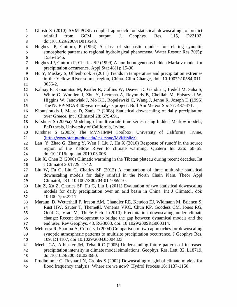
1 2 3 4 5 Table 1 List of stations used in this study. The location of each station is marked in Figure 1 6 using the corresponding numbers given in the first column of the table 7

Station number

Station name

Latitude (°N)

Longitude (°E)

Elevation (m)

1 Maduo 34.92 98.22 4272 2 Renxiamu 34.27 99.20 4211 3 Jimai 33.77 99.65 3969 4 Dari 33.75 99.65 3697 5 Jiuzhi 33.43 101.48 3628 6 Hongyuan 32.80 102.55 3491 7 Nuoergai 33.58 102.97 3439 8 Maqu 33.97 102.08 3400 9 Henan 34.73 101.60 3500 10 Zeku 35.03 101.47 3663 11 Tongde 35.27 100.65 3289 12 Tangnag 35.50 100.65 2665 13 Xinghai 35.58 99.98 3245 14 Gonghe 36.27 100.62 2835

8

Table 2. Comparison of the ways the rainfall occurrence, amount and spatial dependence 9 structure are modeled in these three downscaling methods. 10

Notation SDSM GLIMCLIM NHMM

Precipitation occurrence

depends on current day's predictors and previous day's precipitation occurrence

depends on current day's predictors and 3 previous days' precipitation occurrence

depends only on current day's weather state

Precipitation amount

• using an empirical distribution • separate parameters for each station and each month

• using a gamma distribution with logarithm transformation of the mean being modeled as a linear function of predictors • a constant shape parameter for all stations

• using a gamma distribution • separate parameters for each station and each weather state

Spatial dependence none constant inter-site correlation structure none

11

12

13

17

1

Fig. 1 Map of the study area showing the locations (filled circle) of rain-gauge stations and 2 selected grid points (plus sign) for the NCEP data. Station names refer to Table 1. The smaller 3 map in the upper right corner presents the location the Yellow River source region in China 4 (black shaded area). 5

6

7

Fig. 2 Scatter plots of observed and mean modeled Spearman cross correlation obtained by (a) 8 SDSM, (b) GLIMCLIM and (c) NHMM for the validation period. 9

10

11

18

1

2

3

4 Fig. 3 Observed versus modeled wet spell lengths distribution by SDSM (left), GLIMCLIM 5 (middle) and NHMM (right) for the validation period at representative stations. Station numbers 6 refer to Table 1 and Fig. 1. 7

8

9

10

11 Fig. 4 Observed versus modeled dry spell lengths distribution by SDSM (left), GLIMCLIM 12 (middle) and NHMM (right) for the validation period at representative stations. Station numbers 13 refer to Table 1 and Fig. 1. 14

15

19

1

Fig. 5 Correlation between the simulated and observed summer precipitation for each station 2 during the validation period 1981-1990. Station numbers refer to Table 1 and Fig. 1. 3

4

Fig. 6 Box-plots of bias (percentage difference between observed and median simulated) in 5 downscaled summer precipitation during the validation period 1981-1990. The box-plots depict 6 the range of the bias across 14 stations. The boxes denote the median and interquartile range 7 (IQR). Whiskers extend 1.5 IQR from box ends, with outliers denoted as “◦”. 8

9 Fig. 7 Bias (percentage difference between observed and median simulated) in downscaled 10 summer precipitation from the CGCM3 and ECHAM5 predictors at each station. Station numbers 11 refer to Table 1 and Fig. 1. 12

13

20

1

2

3

4

5

6 Fig. 8 Box plots of projected precipitation indices anomalies (A2, A1B and B1 scenarios, 2046-7 2065 minus 1961-1990) based on downscaled results from CGCM3 and ECHAM5. The box-plots 8 depict the range of projected precipitation anomalies across 14 stations. The boxes denote the 9 median and interquartile range (IQR)). Whiskers extend 1.5 IQR from box ends. Spatial variability 10 can be inferred from the height of the box and whiskers. 11

21

1

2

3

4

5

6

7 Fig. 9 Fitted gamma Probability density functions (PDF) for future (2046-2065) and current 8 (1961-1990) precipitation indices averaged across all stations based on downscaled results from 9 two GCMs. SDSM (left column); GLIMCLIM (middle column); NHMM (right column). C 10 denotes the control climate; A2, A1B and B1 denote the three emission scenarios. 11 12