Download=RomanelliSerioliMantegazza 3OFWorkshop Presentation

3rd OpenFOAM Workshop 11th July 2008

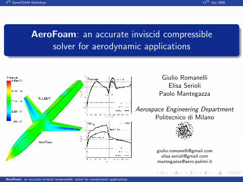
AeroFoam: an accurate inviscid compressiblesolver for aerodynamic applications

Giulio RomanelliElisa Serioli

Paolo Mantegazza

Aerospace Engineering DepartmentPolitecnico di Milano

[email protected]@gmail.com

[email protected]

AeroFoam: an accurate inviscid compressible solver for aerodynamic applications

Introduction Numerical scheme Test problems Work in progress Future work

Table of contents

1 Introduction

2 Numerical scheme

3 Test problems

4 Work in progress

5 Future work



Outline

Objective

Develop a new accurate inviscid compressible Godunov-type coupled solver foraerodynamic (and aeroelastic) applications in transonic and supersonic regime

To begin with

OpenFOAM built-in inviscid compressible segregated (with PISO correction)solvers rhoSonicFoam, rhopSonicFoam and sonicFoam

Previous similar work

centralFoam by L. Gasparini: inviscid compressible central (or central-upwind)coupled solver, 2nd order formulation of Kurganov, Noelle and Petrova (KNP)

GASDYN+OpenFOAM 1D/3D formulation by Dipartimento di Energetica,Politecnico di Milano: inviscid compressible Godunov-type coupled solver,1st order Harten, Lax and vanLeer (HLL/C) Riemann solver



Euler equationsGoverning equations for time-dependent, compressible, ideal (inviscid µ = 0 andnonconducting κ = 0) fluid flows in coupled, integral, conservative form:

V ⊆ RNd

S = ∂V ⊆ RNd−1

β

Sinflow ⊆ S | β · n ≤ 0

n

n

ddt

∫V

udV +

∮S

f(u) · n dS = 0

u(x, 0) = u0(x)

u(x ∈ Sinflow, t) = ub(t)

Conservative variables vector and inviscid flux function tensor:

u =

ρ

m

Et

=

ρ

ρ v

ρe + 12ρ|v|2

f =

m

mρ ⊗m + P [ I ]

mρ (Et + P )

Polytropic Ideal Gas (PIG) thermodynamic model: γ = Cp/Cv, R = Ru/M



FV Framework

Sh = ∂Vh

Ωi Ωj

Γij nij

On each Ωi cell: averaged conservative variablesvector (2×volumeScalarField, 1×volumeVectorField)

Ui(t) =1

|Ωi|

∫Ωi

u(x, t) dV

On each Γij interface: numerical fluxes vector(2×surfaceScalarField, 1×surfaceVectorField)

Fij(t) =1

|Γij |

∫Γij

f(u) · n(x, t) dS

On each Ωi cell: cell-centered spatially discretized Euler equations ODE system

dUi

dt+

1

|Ωi|

Nf∑j=1

|Γij |Fij = 0 Targets:

Monotone and sharp solution

near discontinuities

2nd order of accuracy in space

in smooth flow regions?



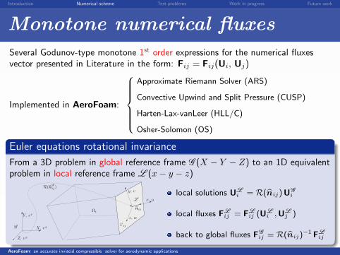
Monotone numerical fluxes

Several Godunov-type monotone 1st order expressions for the numerical fluxesvector presented in Literature in the form: Fij = Fij(Ui, Uj)

Implemented in AeroFoam:

Approximate Riemann Solver (ARS)

Convective Upwind and Split Pressure (CUSP)

Harten-Lax-vanLeer (HLL/C)

Osher-Solomon (OS)

Euler equations rotational invariance

From a 3D problem in global reference frame G (X − Y − Z) to an 1D equivalentproblem in local reference frame L (x− y − z)

PSfrag

Γij

Ωi

x, u

y, v

z, w

X, vX

Y, vY

Z, vZ

R(nG

ij)

nij

G

L

local solutions ULi = R(bnij)UG

i

local fluxes FLij = FL

ij (ULi ,UL

j )

back to global fluxes FGij = R(bnij)

−1 FLij



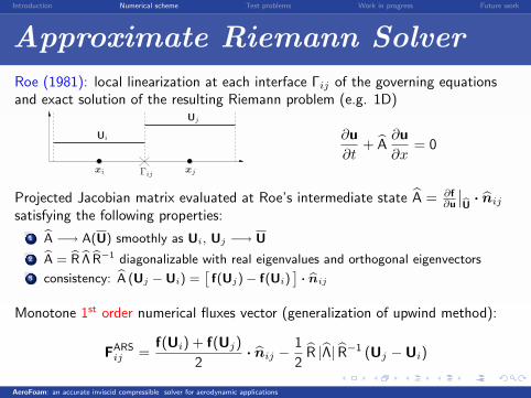
Approximate Riemann Solver

Roe (1981): local linearization at each interface Γij of the governing equationsand exact solution of the resulting Riemann problem (e.g. 1D)

Γijxi xj

Ui

Uj

∂u

∂t+ A

∂u

∂x= 0

Projected Jacobian matrix evaluated at Roe’s intermediate state A = ∂f∂u

∣∣bU · nij

satisfying the following properties:

1 bA −→ A(U) smoothly as Ui, Uj −→ U

2 bA = bR bΛ bR−1 diagonalizable with real eigenvalues and orthogonal eigenvectors

3 consistency: bA (Uj −Ui) =ˆf(Uj)− f(Ui)

˜· bnij

Monotone 1st order numerical fluxes vector (generalization of upwind method):

FARSij =

f(Ui) + f(Uj)

2· nij −

1

2R |Λ| R−1 (Uj −Ui)



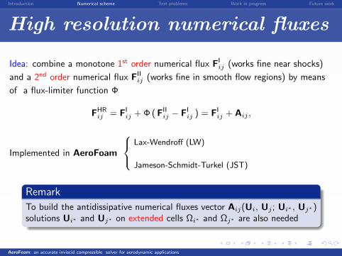
High resolution numerical fluxes

Idea: combine a monotone 1st order numerical flux FIij (works fine near shocks)

and a 2nd order numerical flux FIIij (works fine in smooth flow regions) by means

of a flux-limiter function Φ

FHRij = FI

ij + Φ (FIIij − FI

ij ) = FIij + Aij ,

Implemented in AeroFoam

Lax-Wendroff (LW)

Jameson-Schmidt-Turkel (JST)

Remark

To build the antidissipative numerical fluxes vector Aij(Ui, Uj ; Ui∗ , Uj∗)solutions Ui∗ and Uj∗ on extended cells Ωi∗ and Ωj∗ are also needed



Extended cells connectivity

Idea: continue Ωi and Ωj cells along nij , e.g. Ωj∗ : Ωq ∈ B(Pj) = Ωq|Pj ∈ Ωqsuch that ∆⊥ = ‖(xq − xij)− (xq − xij) · nij nij‖ is minimum

Extended cells connectivity data structures (2× labelField) are initialized in thepre-processing stage with the following algorithms (meshSearch library is used):

Ωi ΩjΩi∗ Ωj∗Pi

Pj

Γijnij

A. Incremental search algorithm(works fine on structured meshes)

initial guess xA = sA bnij

Ωj∗ : Ωq such that xA ∈ Ωq

if Ωj∗ ≡ Ωj update sA = 2 sA

B. Nonincremental search algorithm(works fine on unstructured meshes)

xB = sB bnij where sB = 4|Ωj |/|Γij |Ωj∗ : Ωq such that xB ∈ Ωq



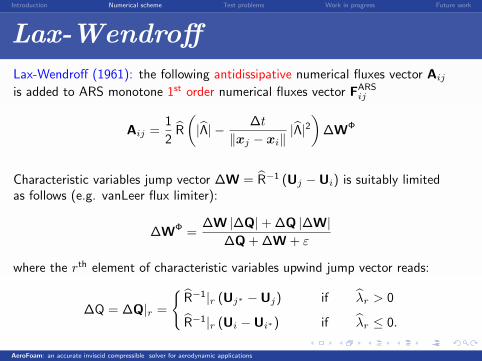
Lax-Wendroff

Lax-Wendroff (1961): the following antidissipative numerical fluxes vector Aij

is added to ARS monotone 1st order numerical fluxes vector FARSij

Aij =1

2R

(|Λ| − ∆t

‖xj − xi‖|Λ|2

)∆WΦ

Characteristic variables jump vector ∆W = R−1 (Uj −Ui) is suitably limitedas follows (e.g. vanLeer flux limiter):

∆WΦ =∆W |∆Q|+ ∆Q |∆W|

∆Q + ∆W + ε

where the rth element of characteristic variables upwind jump vector reads:

∆Q = ∆Q|r =

R−1|r (Uj∗ −Uj) if λr > 0

R−1|r (Ui −Ui∗) if λr ≤ 0.



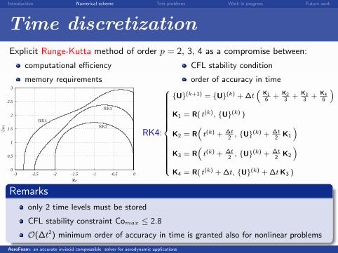
Time discretization

Explicit Runge-Kutta method of order p = 2, 3, 4 as a compromise between:

computational efficiency

memory requirements

CFL stability condition

order of accuracy in time

0

0.5

1

1.5

2

2.5

3

-3 -2.5 -2 -1.5 -1 -0.5 0

ℑm

ℜe

RK2

RK3

RK4

RK4:

8>>>>>>>>>>>>><>>>>>>>>>>>>>:

U(k+1) = U(k) + ∆t“

K16

+ K23

+ K33

+ K46

”K1 = R( t(k), U(k) )

K2 = R“

t(k) + ∆t2

, U(k) + ∆t2

K1

”K3 = R

“t(k) + ∆t

2, U(k) + ∆t

2K2

”K4 = R( t(k) + ∆t, U(k) + ∆t K3 )

Remarks

only 2 time levels must be stored

CFL stability constraint Comax ≤ 2.8

O(∆t2) minimum order of accuracy in time is granted also for nonlinear problems



Boundary conditions

At each boundary interface Γij ∈ Sh = ∂Vh a suitable numerical solution mustbe set on the fictitious or ghost cells ΩGC

j and ΩGCj∗

Ωi

ΩGC

j

Ωi∗

ΩGC

j∗

Γij

nij

vij

Sh = ∂Vh

uij

Characteristic splitting

the number of physical boundaryconditions Nbc equals the number

of negative eigenvalues λr < 0

Physical boundary conditions:Nbc primitive variables assigned

Numerical boundary conditions:Nd+2−Nbc primitive variablesextrapolated



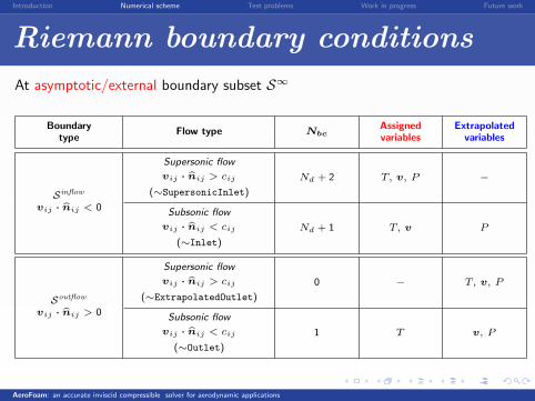
Riemann boundary conditions

At asymptotic/external boundary subset S∞

Boundarytype

Flow type NbcAssignedvariables

Extrapolatedvariables

Sinflow

vij · bnij < 0

Supersonic flow

vij · bnij > cij

(∼SupersonicInlet)

Nd + 2 T, v, P −

Subsonic flow

vij · bnij < cij

(∼Inlet)

Nd + 1 T, v P

Soutflow

vij · bnij > 0

Supersonic flow

vij · bnij > cij

(∼ExtrapolatedOutlet)

0 − T, v, P

Subsonic flow

vij · bnij < cij

(∼Outlet)

1 T v, P



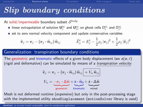
Slip boundary conditions

At solid/impermeable boundary subset Sbody

linear extrapolation of solution UGCj and UGC

j∗ on ghost cells ΩGCj and ΩGC

j∗

set to zero normal velocity component and update conservative variables

vj = vj − (vj · nij) nij Etj = Et

j −1

2ρj |vj |2 +

1

2ρj |vj |2

Generalization: transpiration boundary conditions

The geometric and kinematic effects of a given body displacement law s(x, t)(rigid and deformative) can be simulated by means of a transpiration velocity:

vj = vj − (vj · nij) nij

∣∣∣ + Vn nij

∣∣∣Vn = −vj · ∆n︸︷︷︸

geometric

+ s · n0︸︷︷︸kinematic

+ s · ∆n︸︷︷︸mixed

Mesh is not deformed runtime (expensive) but only in the post-processing stagewith the implemented utility showDisplacement (motionSolver library is used)



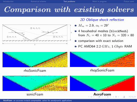
Comparison with existing solvers

L

h

α1 α2

θθ

v1v2

v2

v3

1©

2©

3©M1, P1, T1

M2, P2, T2

M3, P3, T3

2D Oblique shock reflection

M∞ = 2.9, α1 = 29

4 hexahedral meshes (blockMesh)from Nv = 40× 10 to Nv = 320× 80

comparison with exact solution

PC AMD64 2.2 GHz, 1 Gbyte RAM

rhoSonicFoam rhopSonicFoam

sonicFoam AeroFoam



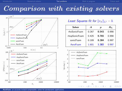
Comparison with existing solvers

0.1

1

10

0.001 0.01 0.1 1

||eh||

L1 [−

]

h [ m ]

O(h)

O(h2)

× 10−2

rhoSonicFoam

rhopSonicFoam

sonicFoam

AeroFoam

Least Squares fit for ‖eh‖L1 − h

Solver A p Rh

rhoSonicFoam 0.267 0.543 0.998

rhopSonicFoam 0.425 0.765 0.998

sonicFoam 0.189 0.384 0.997

AeroFoam 1.601 1.382 0.997

0.01

0.1

1

10

100

100 1000 10000 100000

CPU

tim

e [

s]

Ne

O(Ne)

O(Ne

2)

× 10−1

rhoSonicFoam

rhopSonicFoam

sonicFoam

AeroFoam

0

1

2

3

4

5

6

7

100 1000 10000 100000

Speedup

[−]

Ne

rhoSonicFoam

rhopSonicFoam

sonicFoam



Incompressible limit

2D Fixed cylinder

M∞ = 0.05 !

15K triangular mesh (Gmsh)

comparison with exact solution(potential theory)

single iteration CPUtime = 0.09 s

-1

0

1

2

3

-1 -0.5 0 0.5 1

−C

p [−

]

x/R [−]

CpExact = 1 − 4 sin

2ϑ

AeroFoam

Exact



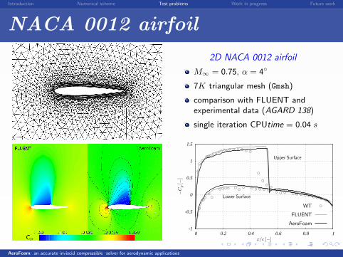
NACA 0012 airfoil

2D NACA 0012 airfoil

M∞ = 0.75, α = 4


comparison with FLUENT andexperimental data (AGARD 138)


-1

-0.5

0

0.5

1

1.5

0 0.2 0.4 0.6 0.8 1

−C

p [−

]

x/c [−]

Upper Surface

Lower Surface

WT

FLUENT

AeroFoam



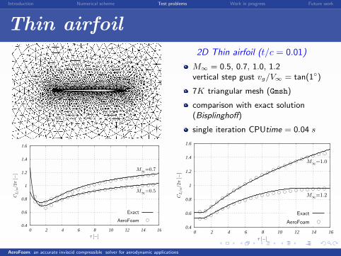
Thin airfoil

2D Thin airfoil (t/c = 0.01)

M∞ = 0.5, 0.7, 1.0, 1.2vertical step gust vg/V∞ = tan(1)


comparison with exact solution(Bisplinghoff)


0.4

0.6

0.8

1

1.2

1.4

1.6

0 2 4 6 8 10 12 14 16

CL

/α/2

π [−

]

τ [−]

M∞

=0.5

M∞

=0.7

Exact

AeroFoam

0.4

0.6

0.8

1

1.2

1.4

1.6

0 2 4 6 8 10 12 14 16

CL

/α/2

π [−

]

τ [−]

M∞

=1.2

M∞

=1.0

Exact

AeroFoam



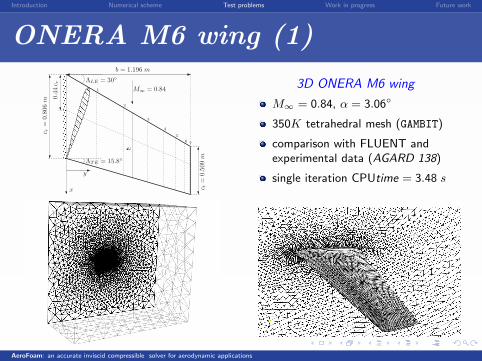
ONERA M6 wing (1)

b = 1.196 m

c r=

0.8

06

m

c t=

0.5

09

m

c

1

2

3

4

5

67

ΛLE = 30

ΛTE = 15.8

M∞ = 0.84

0.4

4c r

x

y

3D ONERA M6 wing

M∞ = 0.84, α = 3.06

350K tetrahedral mesh (GAMBIT)





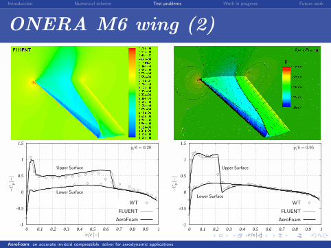
ONERA M6 wing (2)

-1

-0.5

0

0.5

1

1.5

0 0.1 0.2 0.3 0.4 0.5 0.6 0.7 0.8 0.9 1

−C

p [−

]

x/c [−]

Upper Surface

Lower Surface

y/b = 0.20

WT

FLUENT

AeroFoam-1

-0.5

0

0.5

1

1.5

0 0.1 0.2 0.3 0.4 0.5 0.6 0.7 0.8 0.9 1

−C

p [−

]

x/c [−]

Upper Surface

Lower Surface

y/b = 0.95

WT

FLUENT

AeroFoam



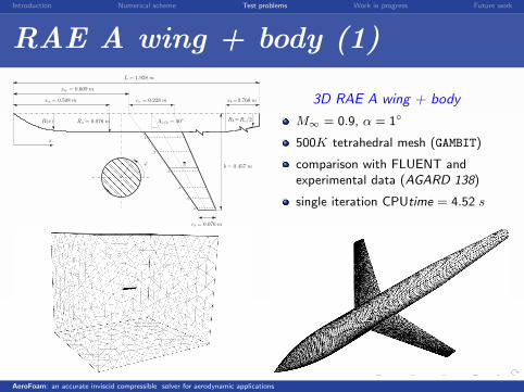
RAE A wing + body (1)

b = 0.457 m

cr = 0.228 m

ct = 0.076 m

L = 1.928 m

xw = 0.609 m

xb =0.760 m

c

Λc/2 = 30

x

Rb =Ro/2

ϕ

R(x) Ro = 0.076 m

xo = 0.508 m

1

2

3

4

5

6

3D RAE A wing + body

M∞ = 0.9, α = 1






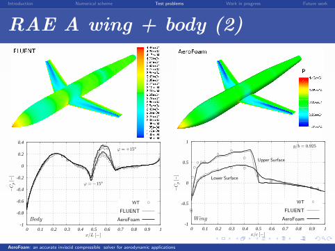
RAE A wing + body (2)

-1

-0.8

-0.6

-0.4

-0.2

0

0.2

0.4

0 0.1 0.2 0.3 0.4 0.5 0.6 0.7 0.8 0.9 1

−C

p [−

]

x/L [−]

ϕ = +15°

ϕ = −15°

Body

WT

FLUENT

AeroFoam-1

-0.5

0

0.5

1

0 0.1 0.2 0.3 0.4 0.5 0.6 0.7 0.8 0.9 1

−C

p [−

]

x/c [−]

Upper Surface

Lower Surface

y/b = 0.925

Wing

WT

FLUENT

AeroFoam



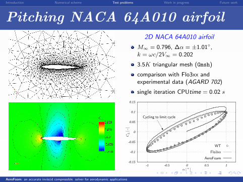
Pitching NACA 64A010 airfoil

2D NACA 64A010 airfoil

M∞ = 0.796, ∆α = ±1.01,k = ωc/2V∞ = 0.202

3.5K triangular mesh (Gmsh)

comparison with Flo3xx andexperimental data (AGARD 702)


-0.15

-0.1

-0.05

0

0.05

0.1

0.15

-1 -0.5 0 0.5 1

CL

[−]

α [ ° ]

Cycling to limit cycle

WT

Flo3xx

AeroFoam



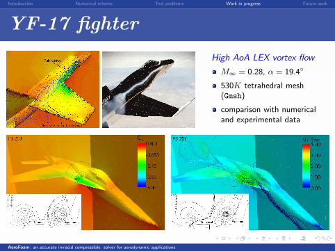
YF-17 fighter

High AoA LEX vortex flow

M∞ = 0.28, α = 19.4

530K tetrahedral mesh(Gmsh)

comparison with numericaland experimental data

q/q∞



AGARD 445.6 wing

Aeroelastic transonic flutter boundary

fluid-structure interaction (FSI)

M∞ = 0.678, 0.960, 1.140, α = 0


comparison with numerical andexperimental data (Langley TDT)

0.2

0.3

0.4

0.5

0.6

0.7

0.6 0.7 0.8 0.9 1 1.1 1.2

Flu

tter index [−

]

M∞

[−]

Experimental

CFL3D

EDGE

FLUENT

AeroFoam

M∞ = 0.960

Mode n1



Future work

Numerical scheme

fully implicit time integration scheme (template for LDUmatrix class needed)

runtime mesh deformation and ALE formulation (dynamicMesh library)

parallelization

Physical models

thermodynamic model of real reacting gas mixture in thermo-chemical equilibrium(important for hypersonic flows)

viscous numerical fluxes and turbulence models (e.g. Spalart-Allmaras)

More 3D test problems (e.g. Piaggio P-180, Apollo reentry capsule)



References

Numerical scheme

M. Feistauer, J. Felcman and I. Straskraba. Mathematical and ComputationalMethods for Compressible Flow. Oxford University Press, 2003

R. J. LeVeque. Numerical Methods for Conservation Laws. Birkhauser Verlag, 1992

Test problems

R. L. Bisplinghoff, H. Ashley and R. L. Halfman. Aeroelasticity. Dover, 1996

Various Authors. “Experimental Data Base for Computer Program Assessment”.AGARD Advisory Report 138, 1979

S. S. Davies and G. N. Malcolm. “Experimental Unsteady Aerodynamics ofConventional and Supercritical Airfoils”. NASA Tech. Memorandum 81221, 1980


Download=RomanelliSerioliMantegazza 3OFWorkshop Presentation

Documents

numerical fluxesvector

solver foraerodynamic

centralupwindcoupled

inviscid flux function

i cell

progress5 future workaerofoam

ij fij

order expressions