Download (168Kb) - Munich Personal RePEc Archive

MPRAMunich Personal RePEc Archive

A model for estimation of the demandfor on-street parking

Edith Madsen and Ismir Mulalic and Ninette Pilegaard

Technical University of Denmark, Technical University of Denmark,Technical University of Denmark

16. December 2013

Online at http://mpra.ub.uni-muenchen.de/52301/MPRA Paper No. 52301, posted 18. December 2013 19:41 UTC

A model for estimation of the demand for

on-street parking∗

Edith Madsen, Ismir Mulalic and Ninette Pilegaard

Technical University of Denmark

December 16, 2013

Abstract

This paper presents a stylized econometric model for the demand

for on-street parking with focus on estimation of the elasticity of de-

mand with respect to the full cost of parking. The full cost of parking

consists of a parking fee and the cost of searching for a vacant parking

space (cruising). The cost of cruising is usually unobserved. Ignoring

this issue implies a downward bias of the elasticity of demand with re-

spect to the total cost of parking since the cost of cruising depends on

the number of cars parked. We also demonstrate that, even when the

cost of cruising is unobserved, the demand elasticity can be identified

by extending the econometric model to include the spatial interaction

between the parking facilities. We illustrate the model with on-street

parking data from Copenhagen and find indications of a somewhat

greater parking demand elasticity than is usually reported in the lit-

erature.

Keywords: on-street parking, demand estimation.

JEL classification: C51, R41, L91.

∗Corresponding author. Tel.: +45 4525 6524. E-mail addresses: [email protected](I. Mulalic), [email protected] (N. Pilegaard), [email protected] (E. Madsen).

1

1 Introduction

Cities around the world use parking policies to regulate the demand for on-

street parking and, to some extent, also the level of urban congestion. It is

therefore of relevance to estimate the sensitivity of the demand for on-street

parking to cost. The full cost of parking (the generalised cost of parking)

consists of a parking fee and in addition the cost of searching for a vacant

parking space (cruising). The cost of cruising is typically unobserved,1 but

ignoring it biases the estimate of the demand elasticity because the cost of

searching for a vacant parking space depends on the number of cars parked,

i.e. the demand for parking. This paper proposes a solution to this problem.

We formulate an econometric model with both parking fees and cruising for

parking as arguments for the demand elasticity for parking. We show how

this demand elasticity can be identified, even in situations where cruising

for parking is unobserved, when the model is extended to include spatial

interaction between the parking facilities.

The economic literature has shown a growing interest for regulatory park-

ing policies. Verhoef et al. (1995) analyse different parking policies as a

substitute to road pricing and find that the use of parking fees is superior to

physical restrictions on parking space supply. Fosgerau & de Palma (2013)

show that workplace parking charging schemes can be used as a substitute

for the time-varying toll to reduce urban congestion. Moreover, it is typically

argued, that parking should be priced at its opportunity cost, just like any

other commodity. Arnott et al. (2005) identify a potential triple dividend

from optimal parking pricing: reduced cruising for parking, reduced conges-

tion (travel time savings), and the use of parking revenues to lower other

taxes (reduced deadweight loss caused by tax distortions). However, in real

life parking facilities are often underpriced (Small & Verhoef, 2007). This

underpricing leads to cruising for parking which is a pure loss from a social

welfare perspective (Shoup (2005) and Calthrop & Proost (2006)). Arnott

& Inci (2006) argue that parking pricing (especially hourly parking fees)

1One exception is Van Ommeren et al. (2012) that examines cruising for parking.However, in this study information on parking fees is not available.

2

has also the downside that it can increase congestion by implying shorter

parking durations and thus increase traffi c congestion by increasing parking

turnover. Arnott et al. (2012) examine the optimal level of curbside parking

capacity when both urban transport and curbside parking are underpriced

and consider the situation where there is garage parking as alternative to the

curbside.

Despite the comprehensive treatment of parking pricing, including the

dependence of the costs of cruising on the number of cars parked, in the the-

oretical urban economics literature (see e.g. Anderson & de Palma (2004)),

there is a rather surprising absence of accurate empirical estimates of the

effect of the cost of parking on the demand for parking. This effect is im-

portant as it is required for a rigorous welfare analysis of a parking policy.

Several studies estimate the price elasticity of demand for parking ignoring

the cost of cruising (see e.g. Kelly & Clinch (2009) and Hensher & King

(2001)). Hence, there is a knowledge gap between the theoretical and empir-

ical literature. This paper goes some way toward filling this gap.

Many cities collect citywide parking data which usually includes the oc-

cupancy rates (the number of cars parked divided by the number of parking

spaces) and the parking fees.2 In this paper, we illustrate our model with

data provided by the city of Copenhagen, covering on-street parking in the

city of Copenhagen, which is a high-density area with strong parking capacity

constraints as often present in high-density metropolitan areas and historical

city centres. This paper provides a framework to clarify the identification

of the effect of the cost of parking consistent with the underlying economic

theory. The framework is suitable for the parking data often collected. We

discuss also the implications for estimation. We show that if only parking

fees are observed, the effect of the cost of parking cannot be identified using a

reduced form parking demand equation. In addition the effect of the parking

fee is always less than the effect of the cost of parking in absolute value. We

also show that the effect of the cost of parking can be identified, even if the

2See e.g. Institute of Transportation Engineers (2012), Puget Sound Regional Council(2012), Seattle Department of Transportation (2011), Felsburg Holt & Ullevig (2009) andNYC Department of Transportation (2009).

3

cost of cruising is unobserved, by extending the econometric model to include

the spatial interaction between the parking facilities (streets). If both the

costs of searching for parking and the parking fees are observed the effect of

the cost of parking can be estimated using instrumental variable techniques.

The next section introduces an econometric model for the demand for

on-street parking; Section 3 presents the empirical illustration and Section 4

concludes.

2 An econometric model of the demand for

parking

In this section we specify an econometric model for the demand for on-street

parking. First, in Section 2.1, we describe a very simple model without

spatial interactions. Then, in Section 2.2, we consider an extension of the

model that takes the spatial interaction into account.

For both models, the demand for on-street parking is described in terms of

the occupancy rate, i.e. the number of parked cars relative to the number of

legal parking lots. The supply of parking lots is assumed to be constant and

thus, the occupancy rate reflects the demand for on-street parking. There

is no modelling of external factors affecting the demand for parking by e.g.

affecting the overall traffi c demand or number of cars. In this way, the model

proposes a partial description without interaction with other sectors. We

also simplify by ignoring the effect on the demand for on-street parking of

other parking alternatives (e.g. private parking houses). We suggest that

this effect is small and thus of little importance, see Section 3.1.

2.1 A simple model

First, let the demand for parking in street i at period t in terms of the

occupancy rate, Oit, (the number of cars parked divided by the number of

4

parking spaces) be given by

Oit = αi + βcit + εit (1)

cit = pit + S (Oit) (2)

where cit is the total cost of parking in street i at period t, αi is a street-

specific fixed effect, and εit is an idiosyncratic error term. The cost cit consists

of a direct cost pit (a parking fee) and an indirect cost, S (Oit), that reflects

the searching costs (cruising) and depends on the occupancy rate Oit. In line

with the literature we assume that the searching cost function S (·) is increas-ing in the occupancy rate, see e.g. Anderson & de Palma (2004). Altogether

equations (1)-(2) express that an increase in the parking fee reduces Oit and

thus increases the number of vacant parking spaces; this in turn implies a

lower cruising time and by that a lower cost of searching. The specification

highlights the fact that the cost of searching, and by that the cost cit, is an

endogenous variable in the parking demand equation.

In our dataset, we do not have any information on searching in terms

of time and costs and therefore we will specify the functional relationship

between the searching costs and the occupancy rate in order to arrive at a

reduced form equation for Oit (see below). It is important to note that if

we did have information on searching then the total cost of parking cit could

be calculated and a valid instrument for cit would be the parking fee pit.

Consequently, the parameter β could be estimated by IV estimation.

The street-specific fixed effects capture all time-invariant differences in the

demand for parking between streets such as the distance to the location of

shopping and leisure activities and the number of residence parking permits

(residents pay an annual fee and in return gain the right to park on-street

in a specific area). Very importantly, the inclusion of street-specific fixed

effects controls for endogeneity of the average parking fee level in a street.

It is typically the case that the fees are higher in the city center where the

demand is also high and vice versa in the areas further away from the city

center. The street-specific fixed effects allow for this type of endogeneity but

excludes the case where a change in the parking fee over time is a response

5

to a change in demand. We find that this assumption is reasonable in most

empirical applications to on-street parking. Typically, these adjustments are

a result of some political decisions rather than demand reactions.3

In order to obtain a reduced form equation for the parking demand in

terms of the occupancy rate Oit we need to specify how the searching costs

depend on the occupancy rate. We assume that the costs of searching are

linear in the occupancy rate:

S (Oit) = a+ bOit where b > 0 (3)

Using (3) it is straightforward to show that the reduced form equation implied

by equations (1)-(2) is

Oit = α̃i + β̃pit + ε̃it (4)

where α̃i = (αi + aβ) / (1− bβ), β̃ = β/ (1− bβ) and ε̃it = εit/ (1− bβ). For

β < 0 then β̃ ∈ ]β, 0] since b > 0 such that the parameter corresponding

to pit in the reduced form equation is less than β in absolute value. The

parameter describes the total effect of increasing the parking fee. The direct

effect is that it will decrease the demand for parking and the indirect effect

is that this in turn will decrease the searching cost which will increase the

demand for parking. The larger the value of b the smaller the absolute value

of the total effect. From this reduced form equation it is not possible to

identify the parameter β in the demand equation and the parameters a and

b in the searching cost function separately. However, if the costs of searching

are piecewise linear in the occupancy rate then all parameters are identified

if there are streets where the occupancy rate is below a threshold value of

the occupancy rate where the cost of searching is zero (see Appendix A).

Obviously, the assumption about the searching cost being linear in the

occupancy rate is strong and a more realistic assumption would be that the

marginal cost of searching is increasing in the occupancy rate. This could for

example be modelled as S (O) = c/ (1−O) where c > 0 as done in Anderson

& de Palma (2004). However, this will lead to a more complicated reduced

3This is reasonably to be the case for our illustrative example from the city of Copen-hagen, see Section 3.1.

6

form equation for the occupancy rate which is not useful in empirical work.

2.2 Spatial interaction between the parking facilities

The framework in Section 2.1 assumes that the demand for parking in a

specific street is independent of the cost of parking in all other streets. This

assumption is obviously not likely to hold in practice since the demand for

parking in a specific street expectedly will also depend on the cost of parking

in neighboring streets. We now extend the model to allow for this. More

formally, we assume that the demand for parking in street i depends on both

the cost of parking in street i and on the cost of parking in neighboring

streets j 6= i. As before, the cost of parking consists of a parking fee and a

searching cost which is increasing in the occupancy rate. The demand for

parking in street i at time t is now given by:

Oit = αi + βcit + γ∑j 6=i

wijcjt + εit (5)

cjt = pjt + S (Ojt) (6)

The parameter γ corresponding to the term∑

j 6=iwijcjt in equation (5) de-

scribes how the demand for parking in a specific street is affected by the

costs of parking in neighboring streets. The spatial weights wij for j 6= i are

prespecified and each weight defines the exact neighboring effect of a specific

street. We use the following geographically derived weights:

wij = exp (−θdij) (7)

where dij is the the shortest route distance between streets i and j, and

θ > 0 is a specified constant (not a parameter that can be estimated). The

weights are exponentially decreasing in the distance and approaches zero as

the distance increases. We use the minimax normalization of the weights (a

common scaling of all weights) and note that this normalization preserves

the symmetry such that wij = wji. For a more extensive discussion of spatial

weights, see e.g. Anselin (1988) and Upton & Fingleton (1985).

The model defined by equations (5)-(6) allows for substitution between

7

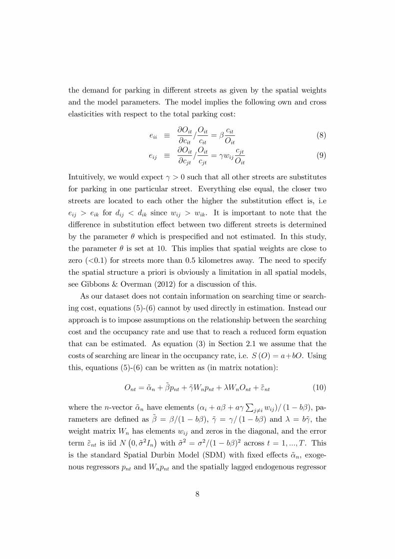
the demand for parking in different streets as given by the spatial weights

and the model parameters. The model implies the following own and cross

elasticities with respect to the total parking cost:

eii ≡∂Oit

∂cit/Oit

cit= β

citOit

(8)

eij ≡∂Oit

∂cjt/Oit

cjt= γwij

cjtOit

(9)

Intuitively, we would expect γ > 0 such that all other streets are substitutes

for parking in one particular street. Everything else equal, the closer two

streets are located to each other the higher the substitution effect is, i.e

eij > eik for dij < dik since wij > wik. It is important to note that the

difference in substitution effect between two different streets is determined

by the parameter θ which is prespecified and not estimated. In this study,

the parameter θ is set at 10. This implies that spatial weights are close to

zero (<0.1) for streets more than 0.5 kilometres away. The need to specify

the spatial structure a priori is obviously a limitation in all spatial models,

see Gibbons & Overman (2012) for a discussion of this.

As our dataset does not contain information on searching time or search-

ing cost, equations (5)-(6) cannot by used directly in estimation. Instead our

approach is to impose assumptions on the relationship between the searching

cost and the occupancy rate and use that to reach a reduced form equation

that can be estimated. As equation (3) in Section 2.1 we assume that the

costs of searching are linear in the occupancy rate, i.e. S (O) = a+bO. Using

this, equations (5)-(6) can be written as (in matrix notation):

Ont = α̃n + β̃pnt + γ̃Wnpnt + λWnOnt + ε̃nt (10)

where the n-vector α̃n have elements (αi + aβ + aγ∑

j 6=iwij)/ (1− bβ), pa-

rameters are defined as β̃ = β/(1 − bβ), γ̃ = γ/ (1− bβ) and λ = bγ̃, the

weight matrix Wn has elements wij and zeros in the diagonal, and the error

term ε̃nt is iid N(0, σ̃2In

)with σ̃2 = σ2/(1 − bβ)2 across t = 1, ..., T . This

is the standard Spatial Durbin Model (SDM) with fixed effects α̃n, exoge-

nous regressors pnt and Wnpnt and the spatially lagged endogenous regressor

8

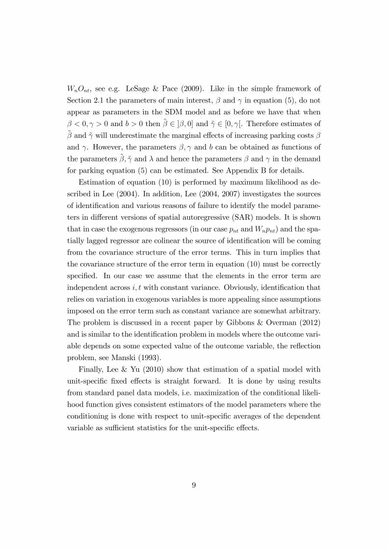
WnOnt, see e.g. LeSage & Pace (2009). Like in the simple framework of

Section 2.1 the parameters of main interest, β and γ in equation (5), do not

appear as parameters in the SDM model and as before we have that when

β < 0, γ > 0 and b > 0 then β̃ ∈ ]β, 0] and γ̃ ∈ [0, γ[. Therefore estimates of

β̃ and γ̃ will underestimate the marginal effects of increasing parking costs β

and γ. However, the parameters β, γ and b can be obtained as functions of

the parameters β̃, γ̃ and λ and hence the parameters β and γ in the demand

for parking equation (5) can be estimated. See Appendix B for details.

Estimation of equation (10) is performed by maximum likelihood as de-

scribed in Lee (2004). In addition, Lee (2004, 2007) investigates the sources

of identification and various reasons of failure to identify the model parame-

ters in different versions of spatial autoregressive (SAR) models. It is shown

that in case the exogenous regressors (in our case pnt andWnpnt) and the spa-

tially lagged regressor are colinear the source of identification will be coming

from the covariance structure of the error terms. This in turn implies that

the covariance structure of the error term in equation (10) must be correctly

specified. In our case we assume that the elements in the error term are

independent across i, t with constant variance. Obviously, identification that

relies on variation in exogenous variables is more appealing since assumptions

imposed on the error term such as constant variance are somewhat arbitrary.

The problem is discussed in a recent paper by Gibbons & Overman (2012)

and is similar to the identification problem in models where the outcome vari-

able depends on some expected value of the outcome variable, the reflection

problem, see Manski (1993).

Finally, Lee & Yu (2010) show that estimation of a spatial model with

unit-specific fixed effects is straight forward. It is done by using results

from standard panel data models, i.e. maximization of the conditional likeli-

hood function gives consistent estimators of the model parameters where the

conditioning is done with respect to unit-specific averages of the dependent

variable as suffi cient statistics for the unit-specific effects.

9

3 Empirical illustration

This section of the paper presents an illustration of the application of the

econometric model. We use parking data from the city of Copenhagen. With

this it is in principle possible to test the model and estimate demand elasticity

of parking with respect to the full cost.

Section 3.1 describes the parking market in the city of Copenhagen. It

also includes a discussion of a number of key assumptions that underlie the

identification of the model and the interpretation of its parameters. The

data set provided by the city of Copenhagen for the analysis is described in

Section 3.2 and estimation results are discussed in Section 3.3. We discuss

our findings on the parking price elasticity, relate our result to the estimates

provided by the existing literature and conclude the section by discussing

the results obtained from estimation of a standard spatial model with street-

specific fixed effects.

3.1 Parking in the city of Copenhagen

About two-third of the parking spaces in the city of Copenhagen are on-

street an hence this is the dominating way of parking (Københavns Kom-

mune (2012)). The city of Copenhagen has, as many other larger cities, a

long history of paid parking (both for publicly provided as well as privately

provided parking places). In 1990 the city of Copenhagen initiated a new

system for payments for parking, where the central city was divided into dif-

ferent zones. The principles of this system is still used today. The purpose

with the system was to reduce the traffi c and the number of parked cars in

the city, especially commuting in cars to workplaces in central Copenhagen

(Københavns Kommune, 2009). In the zonal system all on-street parking

is charged a fee depending on the duration of the parking, time of the day

and the location of the zone. The zones closest to the historical city center

are more expensive. Many other European cities use similar systems where

payment for on-street parking varies across zones and time-intervals.

In the introductory year (2006) the hourly parking fee level was deter-

mined by the level of the observed occupancy rates (demand). The intention

10

was to reduce cruising for parking. In the following years the city authori-

ties increased the parking fees by 1 DKK a year (in nominal terms) without

taking into account the development in the occupancy rates and hence not

as a reaction on the demand.4

At present the zonal system covers three zones: red is the city center with

few residents and many shops, restaurants and offi ces, green and blue have

more residents. These zones has been in use since 2007.

3.2 The data

The data used in the empirical analysis is provided by the city of Copenhagen.

The data is census data and covers the years 2008-2011 with semi-annual

census (in April and September, starting with September 2008). In total we

have 6 census and for each census there are three daily counts (at 12:00, 17:00

and 22:00). The census covers the central Copenhagen (the four parking

zones). For all streets in this area we know the number of legal parking

spaces as well as the number of occupied spaces, for each of the three daily

counts. We do not have information about cruising costs or cruising time.

Furthermore, we do not have information about alternative parking (e.g.

private parking houses and workplace parking).

Table 1 shows the number of parking lots, the number of parked cars, and

the mean occupacy rates for the four parking zones (772 streets) recorded in

April 2011. The number of parking spaces and the distribution among the

zones are almost the same in the three years that we consider.

The parking fees for the zones are shown in Table 2. The parking fee

for the red zone (the city center) is almost three times as high as for the

blue zone. Outside the three zones (the outer) there are generally no fees for

parking. We also see that the real prices have been almost constant for the

years 2008-2011. This obviously represents a limitation for the econometric

analysis.

4Special rules apply for residents in a parking zone such that residents are able to parkclose to their homes on very favorable conditions. The price of a resident parking permitis about € 90 per year per car. The parking permit is connected to a specific car andthere is no limit to the number of residence parking permits available.

11

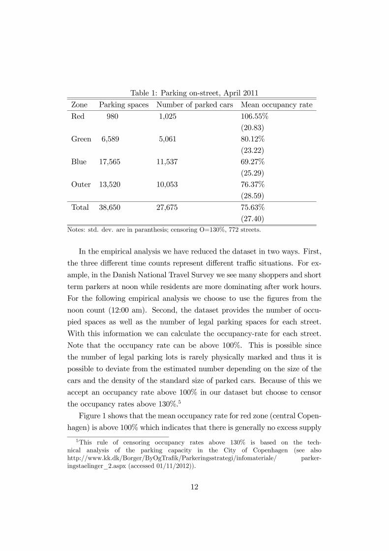
Table 1: Parking on-street, April 2011

Zone Parking spaces Number of parked cars Mean occupancy rate

Red 980 1,025 106.55%

(20.83)

Green 6,589 5,061 80.12%

(23.22)

Blue 17,565 11,537 69.27%

(25.29)

Outer 13,520 10,053 76.37%

(28.59)

Total 38,650 27,675 75.63%

(27.40)Notes: std. dev. are in paranthesis; censoring O=130%, 772 streets.

In the empirical analysis we have reduced the dataset in two ways. First,

the three different time counts represent different traffi c situations. For ex-

ample, in the Danish National Travel Survey we see many shoppers and short

term parkers at noon while residents are more dominating after work hours.

For the following empirical analysis we choose to use the figures from the

noon count (12:00 am). Second, the dataset provides the number of occu-

pied spaces as well as the number of legal parking spaces for each street.

With this information we can calculate the occupancy-rate for each street.

Note that the occupancy rate can be above 100%. This is possible since

the number of legal parking lots is rarely physically marked and thus it is

possible to deviate from the estimated number depending on the size of the

cars and the density of the standard size of parked cars. Because of this we

accept an occupancy rate above 100% in our dataset but choose to censor

the occupancy rates above 130%.5

Figure 1 shows that the mean occupancy rate for red zone (central Copen-

hagen) is above 100% which indicates that there is generally no excess supply

5This rule of censoring occupancy rates above 130% is based on the tech-nical analysis of the parking capacity in the City of Copenhagen (see alsohttp://www.kk.dk/Borger/ByOgTrafik/Parkeringsstrategi/infomateriale/ parker-ingstaelinger_2.aspx (accessed 01/11/2012)).

12

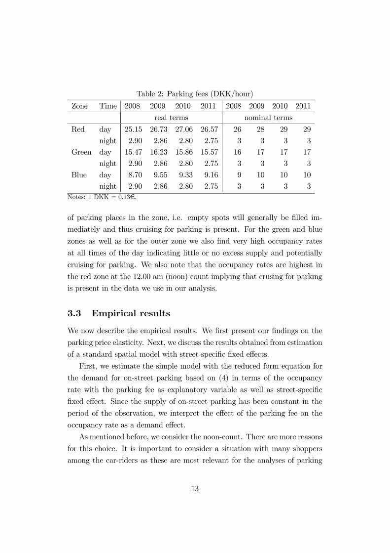
Table 2: Parking fees (DKK/hour)

Zone Time 2008 2009 2010 2011 2008 2009 2010 2011

real terms nominal terms

Red day 25.15 26.73 27.06 26.57 26 28 29 29

night 2.90 2.86 2.80 2.75 3 3 3 3

Green day 15.47 16.23 15.86 15.57 16 17 17 17

night 2.90 2.86 2.80 2.75 3 3 3 3

Blue day 8.70 9.55 9.33 9.16 9 10 10 10

night 2.90 2.86 2.80 2.75 3 3 3 3Notes: 1 DKK = 0.13€.

of parking places in the zone, i.e. empty spots will generally be filled im-

mediately and thus cruising for parking is present. For the green and blue

zones as well as for the outer zone we also find very high occupancy rates

at all times of the day indicating little or no excess supply and potentially

cruising for parking. We also note that the occupancy rates are highest in

the red zone at the 12.00 am (noon) count implying that crusing for parking

is present in the data we use in our analysis.

3.3 Empirical results

We now describe the empirical results. We first present our findings on the

parking price elasticity. Next, we discuss the results obtained from estimation

of a standard spatial model with street-specific fixed effects.

First, we estimate the simple model with the reduced form equation for

the demand for on-street parking based on (4) in terms of the occupancy

rate with the parking fee as explanatory variable as well as street-specific

fixed effect. Since the supply of on-street parking has been constant in the

period of the observation, we interpret the effect of the parking fee on the

occupancy rate as a demand effect.

As mentioned before, we consider the noon-count. There are more reasons

for this choice. It is important to consider a situation with many shoppers

among the car-riders as these are most relevant for the analyses of parking

13

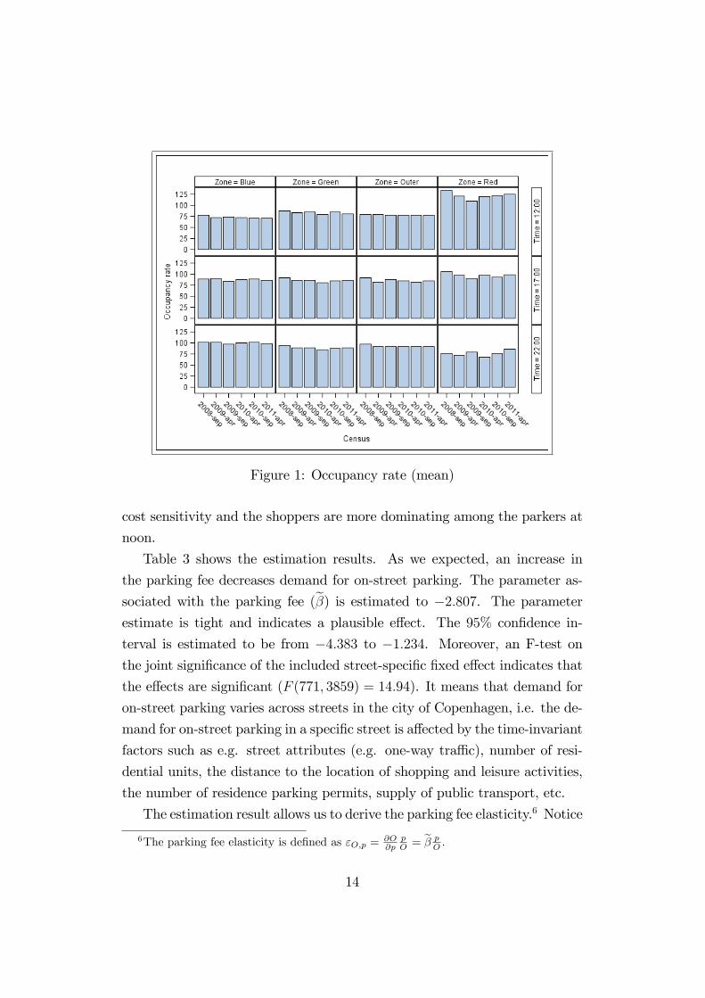
Figure 1: Occupancy rate (mean)

cost sensitivity and the shoppers are more dominating among the parkers at

noon.

Table 3 shows the estimation results. As we expected, an increase in

the parking fee decreases demand for on-street parking. The parameter as-

sociated with the parking fee (β̃) is estimated to −2.807. The parameter

estimate is tight and indicates a plausible effect. The 95% confidence in-

terval is estimated to be from −4.383 to −1.234. Moreover, an F-test on

the joint significance of the included street-specific fixed effect indicates that

the effects are significant (F (771, 3859) = 14.94). It means that demand for

on-street parking varies across streets in the city of Copenhagen, i.e. the de-

mand for on-street parking in a specific street is affected by the time-invariant

factors such as e.g. street attributes (e.g. one-way traffi c), number of resi-

dential units, the distance to the location of shopping and leisure activities,

the number of residence parking permits, supply of public transport, etc.

The estimation result allows us to derive the parking fee elasticity.6 Notice

6The parking fee elasticity is defined as εO,p = ∂O∂p

pO = β̃ p

O .

14

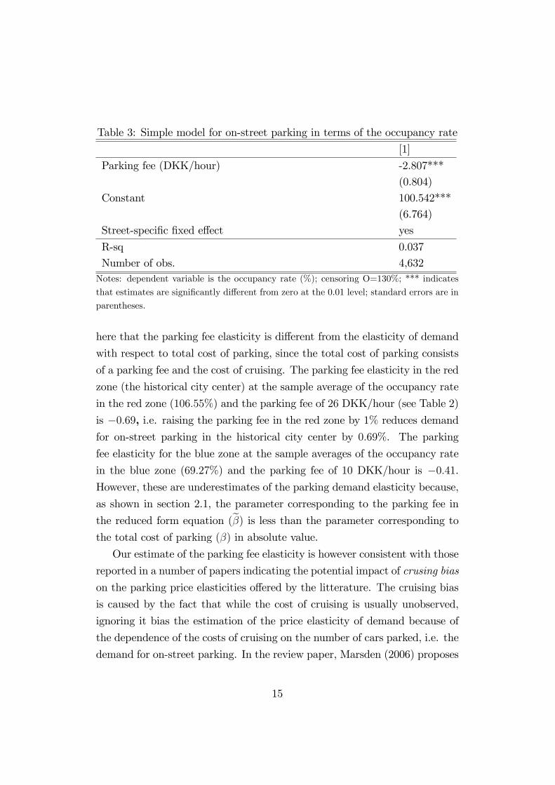
Table 3: Simple model for on-street parking in terms of the occupancy rate

[1]

Parking fee (DKK/hour) -2.807***

(0.804)

Constant 100.542***

(6.764)

Street-specific fixed effect yes

R-sq 0.037

Number of obs. 4,632Notes: dependent variable is the occupancy rate (%); censoring O=130%; *** indicates

that estimates are significantly different from zero at the 0.01 level; standard errors are in

parentheses.

here that the parking fee elasticity is different from the elasticity of demand

with respect to total cost of parking, since the total cost of parking consists

of a parking fee and the cost of cruising. The parking fee elasticity in the red

zone (the historical city center) at the sample average of the occupancy rate

in the red zone (106.55%) and the parking fee of 26 DKK/hour (see Table 2)

is −0.69, i.e. raising the parking fee in the red zone by 1% reduces demand

for on-street parking in the historical city center by 0.69%. The parking

fee elasticity for the blue zone at the sample averages of the occupancy rate

in the blue zone (69.27%) and the parking fee of 10 DKK/hour is −0.41.

However, these are underestimates of the parking demand elasticity because,

as shown in section 2.1, the parameter corresponding to the parking fee in

the reduced form equation (β̃) is less than the parameter corresponding to

the total cost of parking (β) in absolute value.

Our estimate of the parking fee elasticity is however consistent with those

reported in a number of papers indicating the potential impact of crusing bias

on the parking price elasticities offered by the litterature. The cruising bias

is caused by the fact that while the cost of cruising is usually unobserved,

ignoring it bias the estimation of the price elasticity of demand because of

the dependence of the costs of cruising on the number of cars parked, i.e. the

demand for on-street parking. In the review paper, Marsden (2006) proposes

15

a range from −0.6 to −0.1 for the parking demand elasticities (defined in his

study as the percent change in demand of the percent change of parking costs

or parking fees), with −0.3 being the most frequently cited value (see also

TCRP (2005)). Kelly and Clinch (2009) report the average price elasticity

of parking demand (where parking cost is defined as a parking fee per hour)

of −0.29. Moreover, the interpretation of the parking fee elasticity strongly

depends on the assumption with respect to the level of residential parking,

because the estimate of the parking fee elasticity depends on the ratio of the

average parking fee and the average occupancy rate. This occupancy rate

is highly affected by the amount of residential parking as a large number

of parking spaces can be more or less permanently occupied by users with

resident parking permits. Unfortunately, the information on the share of

cars parked using the residential parking permit in the city of Copenhagen is

not available. Based on some Danish experienced practitioners’best guesses

(different analyses conducted by the Municipality of Copenhagen and the

bordering municipality Frederiksberg) this share is expected to be in the

range of 10 − 30%. The parking fee elasticity is then closer to −1. This is

also in line with the usual findings. Hensher and King (2001) propose parking

price elasticity (the percent change in the probability of choosing to park in

a given area of a one percent increase in the hourly parking fee) in the range

from −1.02 to −0.48. Our findings indicate, that due to the cruising bias,

the parking demand elasticity (the car drivers’response to an increase in the

total cost of parking) is most likely larger than proposed in the literature.

Estimation of the reduced form spatial model in equation (10) is in prin-

ciple straight forward, see Section 2.2. However, in practice it turns out to

be diffi cult because in our data set the parking fees at a given point in time

are the same within a specific parking zone. This means that for streets

where the distance to streets in other zones is large the variables pit and∑j 6=i ωijpjt are proportional. In our analysis where we have chosen θ = 10

this is the case for streets where the distance to other zones is greater than

0.5 km. This holds for streets within the center of a zone and for streets on

the boundary of a zone with no border to other zones. It implies that the

variables pnt and Wnpnt are close to being colinear and consequently it is not

16

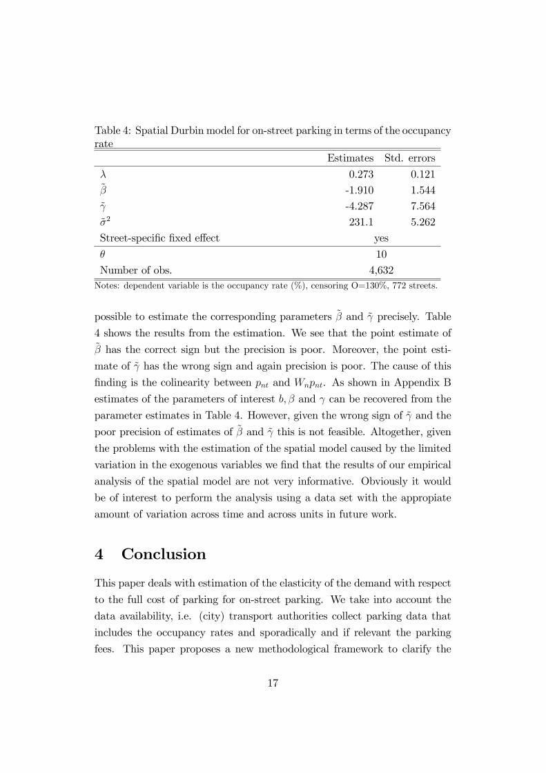
Table 4: Spatial Durbin model for on-street parking in terms of the occupancyrate

Estimates Std. errors

λ 0.273 0.121

β̃ -1.910 1.544

γ̃ -4.287 7.564

σ̃2 231.1 5.262

Street-specific fixed effect yes

θ 10

Number of obs. 4,632Notes: dependent variable is the occupancy rate (%), censoring O=130%, 772 streets.

possible to estimate the corresponding parameters β̃ and γ̃ precisely. Table

4 shows the results from the estimation. We see that the point estimate of

β̃ has the correct sign but the precision is poor. Moreover, the point esti-

mate of γ̃ has the wrong sign and again precision is poor. The cause of this

finding is the colinearity between pnt and Wnpnt. As shown in Appendix B

estimates of the parameters of interest b, β and γ can be recovered from the

parameter estimates in Table 4. However, given the wrong sign of γ̃ and the

poor precision of estimates of β̃ and γ̃ this is not feasible. Altogether, given

the problems with the estimation of the spatial model caused by the limited

variation in the exogenous variables we find that the results of our empirical

analysis of the spatial model are not very informative. Obviously it would

be of interest to perform the analysis using a data set with the appropiate

amount of variation across time and across units in future work.

4 Conclusion

This paper deals with estimation of the elasticity of the demand with respect

to the full cost of parking for on-street parking. We take into account the

data availability, i.e. (city) transport authorities collect parking data that

includes the occupancy rates and sporadically and if relevant the parking

fees. This paper proposes a new methodological framework to clarify the

17

identification of the effect of the cost of parking (consisiting of the costs of

searching for parking (cruising) and a parking fee) on the demand when the

cost of searching is unobserved.

We illustrate the model using on-street data from the city of Copenhagen

for the years 2008-2011. Limitations in the data prevents us from estimating

the elasticity properly but our illustrations suggest that the parking demand

elasticity is most likely larger than the one proposed in the literature.

Our findings have a number of implications. First it demonstrates that

parking fees can potentially be a useful policy instrument to organize the

parking market and to reduce the external costs of traffi c such as congestion

(cruising), air pollution, and other relevant local environmental externalities.

It also demonstrates that, in line with the literature (see Arnott et al., 1991),

a spatially differentiated parking fee is necessary to induce the optimal park-

ing pattern. Second, the proposed empirical methodology can be useful for

the estimation of other similar reduced form demand equation describing the

demand with the constrained capacity. In particular the reduced form de-

mand equation resulting from a bottleneck model is a good example (see e.g.

Arnott et al. (1993)). Finally, the proposed methodology makes it possible

to make a straightforward extension of the demand model to include spatial

interactions. In this way many of the identification problems in applied spa-

tial economics can be avoided.

Acknowledgement 1 The authors thank Mogens Fosgerau, Jos Van Om-meren and Eren Inci for their useful suggestions on an earlier draft and

research assistant Sara Tvile Marker Sørensen for data management. We

are grateful to the city of Copenhagen (Åse Boss Henrichsen and Anders

Møller) for providing the data. Seminar participants at the Kuhmo Nec-

tar Conference on Transportation Economics 2012, LATSIS 2012, and DTU

Transport at the Technical University of Denmark also provided helpful com-

ments. Research support from the Danish Council for Strategic Research is

acknowledged. All remaining errors are the authors’alone.

18

5 Appendices

5.1 Appendix A

Assume now that the costs of searching are piecewise linear in the occupancy

rate

S (Oit) =0 if Oit < Θ

a+ bOit if Oit ≥ Θ(A.1)

It means that the cost of searching is zero when the occupancy rate is less

than a threshold value Θ (e.g. Θ = 70%) and linear and increasing for values

above Θ. This might be a more realistic assumption than having the costs

being linear in the occupancy rate since if the occupancy rate is low then

there will be empty parking spaces and the cost of searching is zero. The

threshold value at Θ reflects that if the occupancy rate is above this level

then it is more likely that all spaces are occupied which implies cruising. Note

also that, as emphasised by Arnott & Inci (2006), given perfect information

about parking spaces and optimal pricing of parking, cruising time is (close

to) zero.

The reduced form for the eq.(A.1) is now given by

Oi =αi + βpi if pi ≥ (Θ− αi) /β

αi+aβ1−bβ + β

1−bβpi if pi < (Θ− αi) /β(A.2)

In this case all parameters are identified if there are streets where the occu-

pancy rate is less than Θ. This identification strategy utilises the fact that

the expression is non-linear in the exogenous variable. The diffi culty is re-

lated to the correct censoring of the occupancy rate. The threshold value Θ

should be selected at the level at which the cost of searching turns to zero.

5.2 Appendix B

This appendix shows how to obtain the parameters b, β and γ from the

parameters β̃, γ̃ and λ that result from estimation of the spatial model in

19

equation (10). The following holds:

b =λ

γ̃

β =β̃

1 + λ/(β̃γ̃)

γ = γ̃ − λβ̃

1 + λ/(β̃γ̃)

References

Anderson, S.P. and A. de Palma. 2004. The economics of pricing parking.

Journal of Urban Economics 55, 1-20.

Anselin, L. 1988. Spatial Econometrics: Methods and Models. Kluwer Aca-

demic, Dordrecht.

Arnott, R., A. de Palma and R. Lindsey. 1993. A Structural Model of Peak-

Period Congestion: A Traffi c Bottleneck with Elastic Demand. The

American Economic Review, vol.83(1), pp. 161-179.

Arnott, R., T. Rave and R. Schöb. 2005. Alleviating Urban Traffi c Conges-

tion. Cambridge, MA, MIT Press.

Arnott, R. and E. Inci. 2006. An integrated model of downtown parking and

traffi c congestion. Journal of Urban Economics 60, 418-442.

Arnott, R., E. Inci and J. Rowse. 2012. Downtown Curbside Parking Capac-

ity, CESifo Working Paper No. 4085.

Arnott, R., A. de Palma and R. Lindsey. 1991. A temporal and spatial equi-

librium analysis of commuter parking. Journal of Public Economics 45,

301-335.

Calthrop, E. and S. Proost. 2006. Regulating on-street parking. Regional

Science and Urban Economics, 36, 29-48.

20

Felsburg Holt & Ullevig. 2009. Tennyson street study area —

parking analysis. Prepared for City and County of Denver.

http://www.denvergov.org/Portals/706/documents/Tennsyson%2038th-

45th%20Parking%20Analysis%20Oct%2009.pdf (accessed 18/11/2012).

Fosgerau, M. and A. de Palma. 2013. The dynamics of urban traffi c conges-

tion and the price of parking. Journal of Public Economics, forthcoming.

Gibbons, S. and H. Overman. 2012. Mostly pointless spatial econometrics.

Journal of Regional Science, vol. 51(2), pp. 172-191.

Glazer, A. and E. Niskanen. 1992. Parking fees and congestion. Regional

Science and Urban Economics, 22, 123-132.

Hensher, D.A. and J. King. 2001. Parking demand and responsiveness to sup-

ply, pricing and location in the Sydney central business district. Trans-

portation Research A 35 (3), pp. 177—196.

Institute of Transportation Engineers. 2012. Parking Occupancy - Inde-

pendent Variables. http://www.ite.org/parkinggeneration/variables.asp

(accessed 18/11/2012).

Kelly, J. and J.P. Clinch. 2009. Temporal variance of revealed preference

on-street parking price elasticity. Transport Policy 16, pp. 193-199.

Københavns Kommune, 2012. Københavns kommunes parkeringsinforma-

tion. www.kk.dk/borger/byogtrafik/parkering (accessed 18/11/2012).

Københavns Kommune, 2009. Adfærdsregulering af trafikken og parkeringen.

Notat 10-03-2009, Teknik- og miljøforvaltningen.

Lee, L. 2004. Asymptotic distribution of quasi-maximum likelihood estima-

tors for spatial autoregressive models. Econometrica 72(6), 1899-1925.

Lee, L. 2007. Identification and estimation of econometric models with group

interactions, contextual factors and fixed effects. Journal of Economet-

rics 140, 333-374.

21

Lee, L. and J. Yu. 2010. Estimation of spatial autoregressive panel data

models wih fixed effects, Journal of Econometrics 154, 165-185.

LeSage, J. and R. K. Pace. 2009. Introduction to Spatial Econometrics. Chap-

man and Hall.

Manski, C. F. 1993. Identification of endogenous social effects: The reflection

problem. Review of Economic Studies 60, 531—542.

Marsden, G. 2006. The evidence base for parking policies– a review. Trans-

port Policy 13, pp. 447-457.

NYC Department of Transportation. 2009. PARK

Smart Greenwich Village Pilot Program — Results.

http://www.nyc.gov/html/dot/downloads/pdf/parksmart_gv_results

_july09.pdf (accessed 18/11/2012).

Puget Sound Regional Council. 2012. Parking Inventory.

http://www.psrc.org/data/transportation/parking-inventory/ (ac-

cessed 18/11/2012).

Seattle Department of Transportation. 2011. Citywide

paid parking study and 2011 rates. Technical re-

port. http://www.seattle.gov/transportation/parking/docs/

ParkingStudyTechRep-final.pdf (accessed 18/11/2012).

Shoup, D.C. 2005. The high cost of free-parking. Planners Press, Chicago.

Small, K.A. and E. T. Verhoef. 2007. The economics of urban transportation.

Routledge.

TCRP, 2005. Parking Prices and Fees: Traveler Response to Transporta-

tion System Changes. Transit Cooperative Research Program Report

95. Transportation Research Board, Washington DC.

Upton, G. J. and B. Fingleton. 1985. Spatial Data Analysis by Example.

Volume 1: Point Pattern and Quantitative Data. Wiley, New York.

22

Van Ommeren, J.N., D. Wentink and P. Rietveld. 2012. Evidence on cruising

for parking. Transportation Research Part A, vol. 46, 1, pp 123-130.

Verhoef, E, P. Nijkamp and P. Rietveld. 1995. The economics of regulatory

parking policies: the (im)possibilities of parking policies in traffi c regu-

lation. Transportation Research Part A, vol. 29A, 2, pp 141-156.

23