Eur. Phys. J. D 22, 163–182 (2003) DOI: 10.1140/epjd/e2003-00012-2 T HE EUROPEAN P HYSICAL JOURNAL D Double Penning trap technique for precise g factor determinations in highly charged ions H. H¨ affner 1,2, a , T. Beier 1 , S. Djeki´ c 2 , N. Hermanspahn 2, b , H.-J. Kluge 1 , W. Quint 1 , S. Stahl 1,2 , J. Verd´ u 2 , T. Valenzuela 2 , and G. Werth 2 , c 1 GSI, Atomic Physics, Planckstr. 1, 64291 Darmstadt, Germany 2 Institut f¨ ur Physik, Universit¨at Mainz, 55099 Mainz, Germany Received 17 June 2002 / Received in final form 13 September 2002 Published online 21 January 2003 – c EDP Sciences, Societ`a Italiana di Fisica, Springer-Verlag 2003 Abstract. We present a detailed description of an experiment to determine the magnetic moment of an electron bound in hydrogen-like carbon. This forms a high-accuracy test of bound-state quantum electro- dynamics. Special emphasis is given to the discussion of systematic uncertainties which limit our present accuracy. The described experimental setup may also be used for the determination of g factors in other highly charged ions. PACS. 32.10.Dk Electric and magnetic moments, polarizability – 06.20.Jr Determination of fundamental constants – 31.30.Jv Relativistic and quantum electrodynamic effects in atoms and molecules 1 Introduction 1.1 General The experimental determination of the magnetic moment (g J factor) of the bound electron in hydrogen-like ions is an important test of Quantum Electrodynamics (QED) in strong Coulomb fields [1–3]. It represents a rather clean test of pure QED effects because it is not very sensitive to nuclear structure effects which usually are more difficult to take into account [4–6]. Precise experimental data on the g J factor of the bound electron in hydrogenic systems have been available until recently only for the hydrogen atom ([7–9] and references therein) and the 4 He + -ion [10]. These results, however, were not sensitive to bound-state QED effects, which are very small at low values of the nuclear charge Z . In addition to these measurements, the magnetic moments of the electrons bound to 207 Pb 81+ and 209 Bi 82+ - nuclei were extracted from lifetime measurements of the excited hyperfine splitting level of the ground state to a precision of about 10 −3 [11–13] which is not sufficient to observe bound-state QED effects. Recently we have published the result of an experiment on the g J factor of hydrogen-like 12 C 5+ using a single ion confined in a Penning ion trap [3]. The precision of a few a Present address: Institut f¨ ur Experimentalphysik, Univer- sit¨at Innsbruck, 6020 Innsbruck, Austria. b Present address: 54 Warrington St., St. Albans, Christchurch 8001, New Zealand. c e-mail: [email protected] parts in 10 9 was sufficient to test bound-state QED cor- rections of order α/π on the 1% level in spite of the rather low value of Z . It was even possible to derive a new value for the mass of the electron [14,15] which is more pre- cise than the current accepted value [16]. An extension of our method to hydrogen-like or lithium-like ions with higher Z values would investigate the bound-state QED contributions even more stringently. In this article we give a detailed description of our experiment with special em- phasis of the possible systematic effects which at present limit our precision. The paper is organized as follows: after a short intro- duction on the measurement principle, we describe the experimental set-up and the basic techniques used for the experiments (Sect. 2). Section 3 describes measurements of the ion’s motional frequencies and the detection of in- duced spin transitions. Section 4 is devoted to a discussion of the systematic uncertainties. 2 Experimental techniques 2.1 Measurement principle The g J factor of an electron is defined in terms of the ratio of its magnetic moment µ to its angular momentum J µ = −g J e 2m e J, (1)

Welcome message from author
This document is posted to help you gain knowledge. Please leave a comment to let me know what you think about it! Share it to your friends and learn new things together.
Transcript
Eur. Phys. J. D 22, 163–182 (2003)DOI: 10.1140/epjd/e2003-00012-2 THE EUROPEAN
PHYSICAL JOURNAL D
Double Penning trap technique for precise g factor determinationsin highly charged ions
H. Haffner1,2,a, T. Beier1, S. Djekic2, N. Hermanspahn2,b, H.-J. Kluge1, W. Quint1, S. Stahl1,2, J. Verdu2,T. Valenzuela2, and G. Werth2,c
1 GSI, Atomic Physics, Planckstr. 1, 64291 Darmstadt, Germany2 Institut fur Physik, Universitat Mainz, 55099 Mainz, Germany
Received 17 June 2002 / Received in final form 13 September 2002Published online 21 January 2003 – c© EDP Sciences, Societa Italiana di Fisica, Springer-Verlag 2003
Abstract. We present a detailed description of an experiment to determine the magnetic moment of anelectron bound in hydrogen-like carbon. This forms a high-accuracy test of bound-state quantum electro-dynamics. Special emphasis is given to the discussion of systematic uncertainties which limit our presentaccuracy. The described experimental setup may also be used for the determination of g factors in otherhighly charged ions.
PACS. 32.10.Dk Electric and magnetic moments, polarizability – 06.20.Jr Determination of fundamentalconstants – 31.30.Jv Relativistic and quantum electrodynamic effects in atoms and molecules
1 Introduction
1.1 General
The experimental determination of the magnetic moment(gJ factor) of the bound electron in hydrogen-like ions isan important test of Quantum Electrodynamics (QED) instrong Coulomb fields [1–3]. It represents a rather cleantest of pure QED effects because it is not very sensitive tonuclear structure effects which usually are more difficult totake into account [4–6]. Precise experimental data on thegJ factor of the bound electron in hydrogenic systems havebeen available until recently only for the hydrogen atom([7–9] and references therein) and the 4He+-ion [10]. Theseresults, however, were not sensitive to bound-state QEDeffects, which are very small at low values of the nuclearcharge Z. In addition to these measurements, the magneticmoments of the electrons bound to 207Pb81+ and 209Bi82+-nuclei were extracted from lifetime measurements of theexcited hyperfine splitting level of the ground state to aprecision of about 10−3 [11–13] which is not sufficient toobserve bound-state QED effects.
Recently we have published the result of an experimenton the gJ factor of hydrogen-like 12C5+ using a single ionconfined in a Penning ion trap [3]. The precision of a few
a Present address: Institut fur Experimentalphysik, Univer-sitat Innsbruck, 6020 Innsbruck, Austria.
b Present address: 54 Warrington St., St. Albans,Christchurch 8001, New Zealand.
c e-mail: [email protected]
parts in 109 was sufficient to test bound-state QED cor-rections of order α/π on the 1% level in spite of the ratherlow value of Z. It was even possible to derive a new valuefor the mass of the electron [14,15] which is more pre-cise than the current accepted value [16]. An extensionof our method to hydrogen-like or lithium-like ions withhigher Z values would investigate the bound-state QEDcontributions even more stringently. In this article we givea detailed description of our experiment with special em-phasis of the possible systematic effects which at presentlimit our precision.
The paper is organized as follows: after a short intro-duction on the measurement principle, we describe theexperimental set-up and the basic techniques used for theexperiments (Sect. 2). Section 3 describes measurementsof the ion’s motional frequencies and the detection of in-duced spin transitions. Section 4 is devoted to a discussionof the systematic uncertainties.
2 Experimental techniques
2.1 Measurement principle
The gJ factor of an electron is defined in terms of the ratioof its magnetic moment µ to its angular momentum J
µ = −gJe
2meJ, (1)
164 The European Physical Journal D
where e is the (positive) charge of the electron and me itsmass. The energy difference ∆E between the two orienta-tions of the electron spin in a magnetic field B = Bzez is
∆E = −µ ·B = gJe
2meBz. (2)
Introducing the cyclotron frequency ωec = (e/me) × Bz
and the Larmor precession frequency ωL = ∆E/ of theelectron, the gJ factor can be written as
gJ = 2ωL
ωec
· (3)
Thus the gJ factor of the electron can be determined froma measurement of the Larmor precession frequency andthe cyclotron frequency of the electron.
In our case the electron is bound to a nucleus andtherefore its cyclotron frequency is not directly accessible.One solution would be to store a free electron and measurethe cyclotron frequency separately. This would, however,have some drawbacks due to the opposite charge of theelectron compared to the ion: the ion and the electroncannot be stored at the same time in the same trap and themeasurement of the two frequencies requires a change inthe trapping voltage (e.g. [17]). Contact potentials, patcheffects, and defects in the metal lattice of the trap materialmight result in different positions of the potential energyminima for the ion and the electron, and the two particleswould be located at different regions in the trap. If themagnetic field is not perfectly homogeneous this then leadsto a different field strength experienced by the ion and theelectron.
To avoid these complications we instead measure thecyclotron frequency ωc of the ion. Inserting ωc in equa-tion (3) yields
gJ = 2ωL
ωc
ωc
ωec
· (4)
ωc/ωec in the same magnetic field is directly related to the
mass ratio of the two particles. For 12C5+ it was obtainedfrom a measurement on carbon ions at the University ofWashington [17,18] with a Penning-trap mass spectrome-ter on which the current CODATA value for the electronmass is based [16]. Together with the binding energies alsotaken from [16] we get
ωc(12C5+)/ωec = 0.000 228 627 210 33 (50). (5)
Equation (4) shows that to measure the gJ factor of thebound electron only the frequency ratio ωL/ωc has to bedetermined.
2.2 Our setup
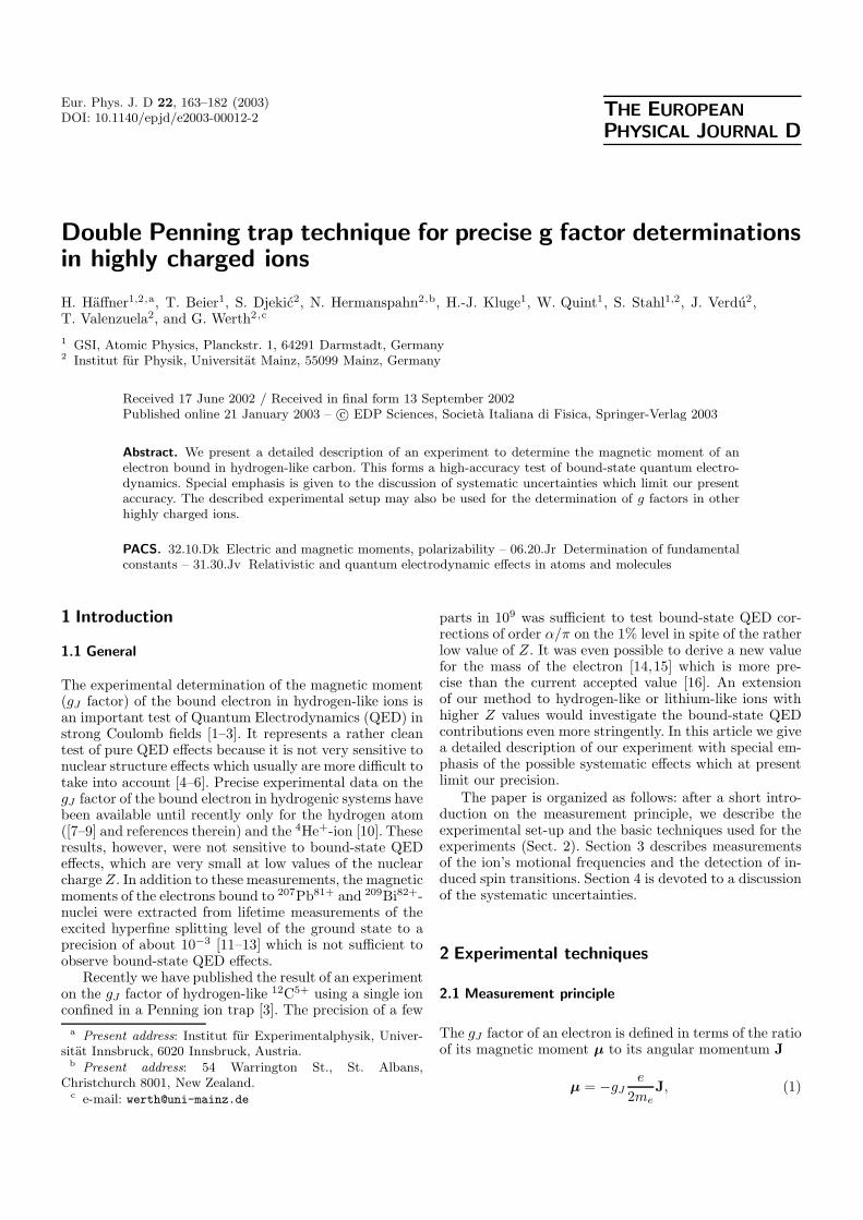
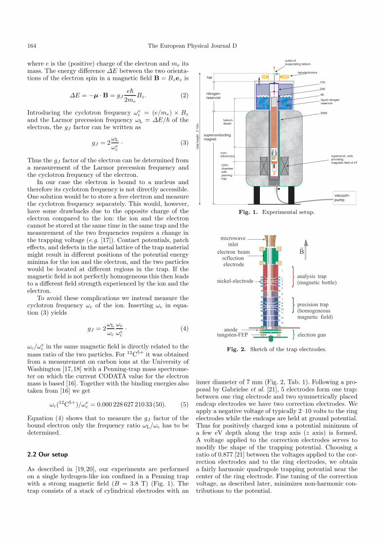
As described in [19,20], our experiments are performedon a single hydrogen-like ion confined in a Penning trapwith a strong magnetic field (B = 3.8 T) (Fig. 1). Thetrap consists of a stack of cylindrical electrodes with an
Fig. 1. Experimental setup.
Fig. 2. Sketch of the trap electrodes.
inner diameter of 7 mm (Fig. 2, Tab. 1). Following a pro-posal by Gabrielse et al. [21], 5 electrodes form one trap:between one ring electrode and two symmetrically placedendcap electrodes we have two correction electrodes. Weapply a negative voltage of typically 2–10 volts to the ringelectrodes while the endcaps are held at ground potential.Thus for positively charged ions a potential minimum ofa few eV depth along the trap axis (z axis) is formed.A voltage applied to the correction electrodes serves tomodify the shape of the trapping potential. Choosing aratio of 0.877 [21] between the voltages applied to the cor-rection electrodes and to the ring electrodes, we obtaina fairly harmonic quadrupole trapping potential near thecenter of the ring electrode. Fine tuning of the correctionvoltage, as described later, minimizes non-harmonic con-tributions to the potential.
H. Haffner et al.: Double Penning trap technique 165
Table 1. Electrode dimensions. All the electrodes have aninner diameter of 7 mm.
Electrode number (see Fig. 2) Length [mm]1 9.342 2.753 0.924 2.755 4.606 5.067 4.838 2.759 0.9210 2.7511 4.8312 3.6813 5.06
As seen in Figure 2, we have two traps of identical ge-ometry spaced by a 1 cm long separation electrode. Thedifference between the two traps is that the ring electrodeof the upper trap is made from nickel while all other elec-trodes are oxygen-free (OFHC) copper. The whole deviceis gold coated to avoid surface charges. The nickel ring in-troduces an inhomogeneity in the trap’s magnetic field,needed to analyze the spin direction of the stored ion(Sect. 3.2). Therefore we call the corresponding trap the“analysis trap”. We term the trap with the homogeneousmagnetic field the “precision trap”. At the lower end of thestack of electrodes we have a field emission cathode. Emit-ted electrons are accelerated to a few hundred electronvolts, pass through the trap arrangement and are reflectedby an additional electrode at the upper end. Coulomb in-teractions between the electrons cause the beam to expandand to hit a pellet near the field emission cathode. De-pending on the electron energy, ions of the pellet materialas well as impurities at different charge states are releasedfrom the surface, drawn into the electron beam and ion-ized further. Some of them are confined in the precisiontrap. In order to achieve long storage times it is essential tooperate the trap in extremely high vacuum since the mainloss mechanism is charge exchange with a neutral parti-cle. The trap’s housing is kept in thermal contact with aliquid helium reservoir. Cryopumping removes essentiallyall background molecules. From extended measurementson a cloud of stored 12C5+ ions we found that the storagetime is longer than one year. We derive that the residualpressure in the trap’s container is below 10−16 mbar. Thisassumes a value of σ = 1.35 × 10⁻¹⁴ cm2 for the C5+ toHe charge exchange cross-section [22].
Our magnetic field is provided by a standard supercon-ducting NMR magnet from Oxford Instruments. It has avertically oriented room temperature bore into which theapparatus is inserted. The apparatus is shown in Figure 1.It consists of two Dewar vessels, electronics and the vac-uum chamber containing the trap. Liquid helium coolsthe apparatus down to 4 K. Electronic circuits [23] for iondetection are placed within 20 cm of the traps to avoid
parasitic capacitances of the cables. They consist mainlyout of three high-Q-r.f. amplifiers for ion detection.
2.3 Frequencies in an ideal and a physical Penning trap
The motion of a single ion in the Penning trap is well un-derstood (e.g. [24]). The solution of the equation of motionin an ideal quadrupole potential and a superposed homo-geneous magnetic field yields three harmonic oscillationswith frequencies
ω+ =ωc
2+
√ωc
2
4− ωz
2
2(6)
ω− =ωc
2−√
ωc2
4− ωz
2
2(7)
ωz =
√eU
md2, (8)
where U is the applied voltage, d the characteristic trap
dimension (defined by d =√
12 (z0
2 + ρ02
2 ) where 2z0 isthe distance between the two endcaps and ρ0 is the ringradius [21]) and ωc the ion’s cyclotron frequency. ω+,ωz, ω− refer to the perturbed cyclotron, axial, and mag-netron oscillations, respectively. For the case of 12C5+ ina field of 3.8 T, U ≈ 13 V and d = 3 mm, we haveω+ ≈ 2π× 24 MHz, ωz ≈ 2π× 1 MHz, ω− ≈ 2π× 20 kHz.The unperturbed cyclotron frequency ωc is not an eigen-frequency of the ion motion, but the ratio ωL/ωc is re-quired to determine the g factor (cf. Eq. (4)).
There are several ways to derive ωc from measuredfrequencies. We choose the so-called invariance theo-rem [24,25]
ωc2 = ω+
2 + ωz2 + ω−2 , (9)
because it is rather insensitive to trap imperfections, suchas an ellipticity of the trap or a tilt of the trap with respectto the magnetic field.
The eigenfrequencies of an ion in a non-ideal trappotential are shifted compared to the values given inequations (6–8). These shifts have been calculated by sev-eral authors [24,36–38]. The perturbations arise from aslightly inhomogeneous magnetic field, anharmonicities inthe electrostatic potential and a small tilt between thetrap axis and the magnetic field direction.
The axially symmetric potential Φ(z, r) can be writtenas a series expansion in Legendre polynomials Pl
Φ(z, r) =∞∑l=0
Cl
( r
d
)l
Pl
(z√
r2 + z2
)· (10)
The leading term is a quadrupole potential (l = 2) whichdepends quadratically on the coordinates. Odd terms inthe expansion are very small because of the mirror sym-metry of the device with respect to the center plane. Inaddition, the length of the electrodes is chosen such thatthe octupole (C4) and dodecapole (C6) contributions to
166 The European Physical Journal D
the trapping potential are simultaneously minimized [21].For the remaining frequency shifts we consider only theoctupole term
∆V = V0C4
z4 − 2z2r2 + 38r4
2d4· (11)
Similarly the magnetic field can be expanded. For our pur-poses it is sufficient to take only a quadratic componentin the magnetic field (magnetic bottle) into account
∆B = B2
[(z2 − r2/2)ez − zr
]. (12)
The change in the magnetron motion is very small andcan be neglected. Then we consider only the axial andperturbed cyclotron motions. The shift ∆ωz of the axialfrequency is given by [24]
∆ωz
ωz=
32
C4
C2
1Emax
Ez +1
mω2z
B2
B0E+, (13)
Ez is the total energy in the axial motion, E+ the cor-responding value in the cyclotron motion. Emax denotesaxial well depth. For constant axial energy, we obtain alinear dependence of the axial frequency on the cyclotronenergy
E+ = mωzB0
B2∆ωz. (14)
This relation is used in our experiment to obtain valuesfor the cyclotron energies from measurements of axial fre-quencies.
For the perturbed cyclotron frequency ω+, we get
∆ω+
ω+= − 1
mω2+
B2
B0E+ +
1mω2
z
B2
B0Ez . (15)
This shift arises from variations in the magnetic field inthe different space regions encountered by the ion at dif-ferent energies. Finally the Larmor-precession frequencyis affected by the magnetic field’s inhomogeneity
∆ωL
ωL= − 1
mω2+
B2
B0E+ +
1mω2
z
B2
B0Ez . (16)
2.4 Axial detection
Oscillating ions induce image charges in the trap elec-trodes. For the axial motion, this leads to an oscillatingcurrent I = dQ/dt = (q/d)z between the trap electrodes,where q is the charge of the ion and z its velocity. We con-nect one of the correction electrodes to a resonant circuit,while all other electrodes are at a.c. ground potential. Res-onant circuits are placed very close to the trap and held atliquid helium temperature. Each circuit consists of a su-perconducting coil and the trap electrodes as capacitance.For the analysis trap we achieve a quality factor Q = 2 500and a corresponding resonance resistance of R = 20 MΩ.The parameters for the precision trap are Q = 1 000 and
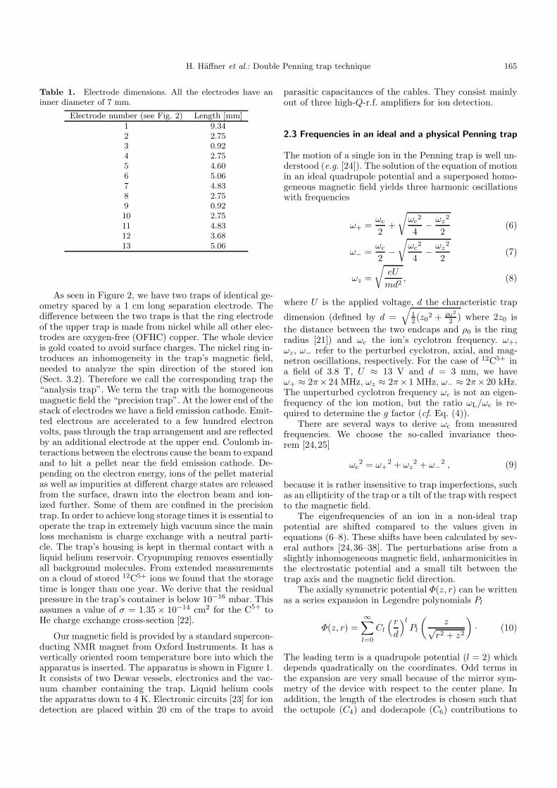
Fig. 3. Axial signals of different ion species stored simultane-ously. Various charge states of C, O, S and Si can be identified.
R = 10 MΩ. If we tune the trap voltage to such a valuethat the ions axial frequency coincides with the resonantfrequency of the circuit, the induced current leads to avoltage drop across the circuit of a few nV for a singletrapped ion. The induced voltage is inductively coupledto a field-effect transistor. To avoid carrier freeze-out at4 K, we use GaAs transistors. Figure 3 shows axial signalsfrom several ion species and charge states simultaneouslypresent in the trap. They are sequentially brought intoresonance with the detection circuit by ramping the trapvoltage. For identification of the different species we usedequation (8) which allows to calculate the axial frequen-cies sufficiently accurate. For signals like those shown inFigure 3, the axial ion energy is of the order of an eV.
2.5 Radial detection
As in the case of the axial motion, the ion oscillation inthe radial plane at frequency ω+ induces image charges inthe trap electrodes. We use one of the compensation elec-trodes for detection of ω+. It is split in two segments whichare connected to a resonant circuit. Thus, the induced cur-rent can be observed. In contrast to the axial resonance,fine tuning of the ion oscillation frequency with the mag-netic field is not possible since the required stability ofour magnetic field does not allow any variation. Thereforewe choose a modest Q = 400 for our circuit at 24 MHz,which is the approximate cyclotron frequency of 12C5+ inour field of 3.8 tesla. The rather low Q-value makes thefrequency setting not too difficult. Furthermore we addedseveral GaAs switching capacities to the circuit to allowchanges of the circuit frequency in discrete steps. Figure 4shows a Fourier transform of the induced current in theradial circuit. It exhibits the signals from 6 12C5+ ions.The ions have slightly different frequencies since they aremoving in different orbits in the inhomogeneous magneticfield. Ions moving faster (having a larger cyclotron or-bit) produce a stronger signal. Typical ion energies in thismeasurement are about 1 keV. In this case the distance
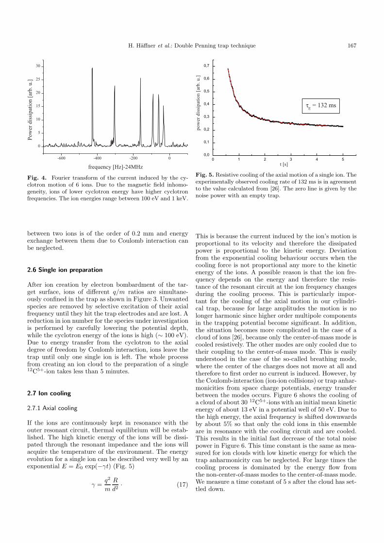
H. Haffner et al.: Double Penning trap technique 167
Fig. 4. Fourier transform of the current induced by the cy-clotron motion of 6 ions. Due to the magnetic field inhomo-geneity, ions of lower cyclotron energy have higher cyclotronfrequencies. The ion energies range between 100 eV and 1 keV.
between two ions is of the order of 0.2 mm and energyexchange between them due to Coulomb interaction canbe neglected.
2.6 Single ion preparation
After ion creation by electron bombardment of the tar-get surface, ions of different q/m ratios are simultane-ously confined in the trap as shown in Figure 3. Unwantedspecies are removed by selective excitation of their axialfrequency until they hit the trap electrodes and are lost. Areduction in ion number for the species under investigationis performed by carefully lowering the potential depth,while the cyclotron energy of the ions is high (∼ 100 eV).Due to energy transfer from the cyclotron to the axialdegree of freedom by Coulomb interaction, ions leave thetrap until only one single ion is left. The whole processfrom creating an ion cloud to the preparation of a single12C5+-ion takes less than 5 minutes.
2.7 Ion cooling
2.7.1 Axial cooling
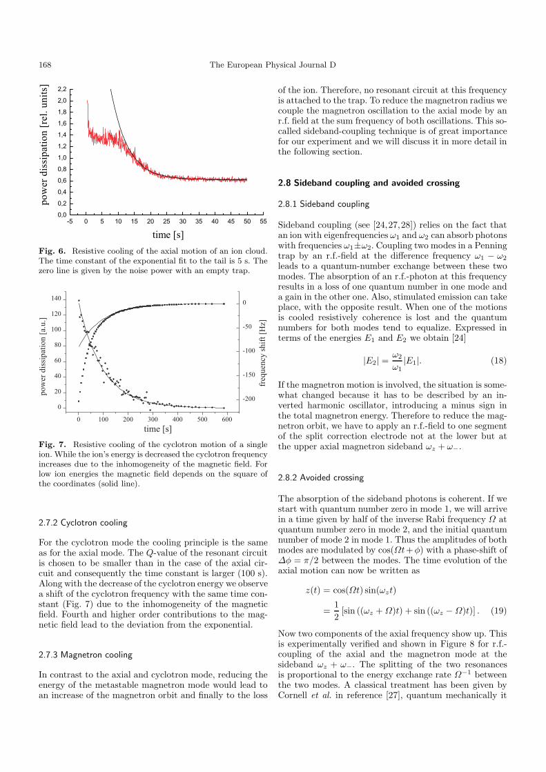
If the ions are continuously kept in resonance with theouter resonant circuit, thermal equilibrium will be estab-lished. The high kinetic energy of the ions will be dissi-pated through the resonant impedance and the ions willacquire the temperature of the environment. The energyevolution for a single ion can be described very well by anexponential E = E0 exp(−γt) (Fig. 5)
γ =q2
m
R
d2· (17)
τ
Fig. 5. Resistive cooling of the axial motion of a single ion. Theexperimentally observed cooling rate of 132 ms is in agreementto the value calculated from [26]. The zero line is given by thenoise power with an empty trap.
This is because the current induced by the ion’s motion isproportional to its velocity and therefore the dissipatedpower is proportional to the kinetic energy. Deviationfrom the exponential cooling behaviour occurs when thecooling force is not proportional any more to the kineticenergy of the ions. A possible reason is that the ion fre-quency depends on the energy and therefore the resis-tance of the resonant circuit at the ion frequency changesduring the cooling process. This is particularly impor-tant for the cooling of the axial motion in our cylindri-cal trap, because for large amplitudes the motion is nolonger harmonic since higher order multipole componentsin the trapping potential become significant. In addition,the situation becomes more complicated in the case of acloud of ions [26], because only the center-of-mass mode iscooled resistively. The other modes are only cooled due totheir coupling to the center-of-mass mode. This is easilyunderstood in the case of the so-called breathing mode,where the center of the charges does not move at all andtherefore to first order no current is induced. However, bythe Coulomb-interaction (ion-ion collisions) or trap anhar-monicities from space charge potentials, energy transferbetween the modes occurs. Figure 6 shows the cooling ofa cloud of about 30 12C5+-ions with an initial mean kineticenergy of about 13 eV in a potential well of 50 eV. Due tothe high energy, the axial frequency is shifted downwardsby about 5% so that only the cold ions in this ensembleare in resonance with the cooling circuit and are cooled.This results in the initial fast decrease of the total noisepower in Figure 6. This time constant is the same as mea-sured for ion clouds with low kinetic energy for which thetrap anharmonicity can be neglected. For large times thecooling process is dominated by the energy flow fromthe non-center-of-mass modes to the center-of-mass mode.We measure a time constant of 5 s after the cloud has set-tled down.
168 The European Physical Journal D
Fig. 6. Resistive cooling of the axial motion of an ion cloud.The time constant of the exponential fit to the tail is 5 s. Thezero line is given by the noise power with an empty trap.
Fig. 7. Resistive cooling of the cyclotron motion of a singleion. While the ion’s energy is decreased the cyclotron frequencyincreases due to the inhomogeneity of the magnetic field. Forlow ion energies the magnetic field depends on the square ofthe coordinates (solid line).
2.7.2 Cyclotron cooling
For the cyclotron mode the cooling principle is the sameas for the axial mode. The Q-value of the resonant circuitis chosen to be smaller than in the case of the axial cir-cuit and consequently the time constant is larger (100 s).Along with the decrease of the cyclotron energy we observea shift of the cyclotron frequency with the same time con-stant (Fig. 7) due to the inhomogeneity of the magneticfield. Fourth and higher order contributions to the mag-netic field lead to the deviation from the exponential.
2.7.3 Magnetron cooling
In contrast to the axial and cyclotron mode, reducing theenergy of the metastable magnetron mode would lead toan increase of the magnetron orbit and finally to the loss
of the ion. Therefore, no resonant circuit at this frequencyis attached to the trap. To reduce the magnetron radius wecouple the magnetron oscillation to the axial mode by anr.f. field at the sum frequency of both oscillations. This so-called sideband-coupling technique is of great importancefor our experiment and we will discuss it in more detail inthe following section.
2.8 Sideband coupling and avoided crossing
2.8.1 Sideband coupling
Sideband coupling (see [24,27,28]) relies on the fact thatan ion with eigenfrequencies ω1 and ω2 can absorb photonswith frequencies ω1±ω2. Coupling two modes in a Penningtrap by an r.f.-field at the difference frequency ω1 − ω2
leads to a quantum-number exchange between these twomodes. The absorption of an r.f.-photon at this frequencyresults in a loss of one quantum number in one mode anda gain in the other one. Also, stimulated emission can takeplace, with the opposite result. When one of the motionsis cooled resistively coherence is lost and the quantumnumbers for both modes tend to equalize. Expressed interms of the energies E1 and E2 we obtain [24]
|E2| =ω2
ω1|E1|. (18)
If the magnetron motion is involved, the situation is some-what changed because it has to be described by an in-verted harmonic oscillator, introducing a minus sign inthe total magnetron energy. Therefore to reduce the mag-netron orbit, we have to apply an r.f.-field to one segmentof the split correction electrode not at the lower but atthe upper axial magnetron sideband ωz + ω−.
2.8.2 Avoided crossing
The absorption of the sideband photons is coherent. If westart with quantum number zero in mode 1, we will arrivein a time given by half of the inverse Rabi frequency Ω atquantum number zero in mode 2, and the initial quantumnumber of mode 2 in mode 1. Thus the amplitudes of bothmodes are modulated by cos(Ωt+φ) with a phase-shift of∆φ = π/2 between the modes. The time evolution of theaxial motion can now be written as
z(t) = cos(Ωt) sin(ωzt)
=12
[sin ((ωz + Ω)t) + sin ((ωz − Ω)t)] . (19)
Now two components of the axial frequency show up. Thisis experimentally verified and shown in Figure 8 for r.f.-coupling of the axial and the magnetron mode at thesideband ωz + ω−. The splitting of the two resonancesis proportional to the energy exchange rate Ω−1 betweenthe two modes. A classical treatment has been given byCornell et al. in reference [27], quantum mechanically it
H. Haffner et al.: Double Penning trap technique 169
Fig. 8. Fourier spectrum of the axial motion without (up-per curve) and with (lower curve) sideband excitation at thefrequency ωz + ω−. The splitting of the axial frequency is notsymmetric due to a slight detuning of the sideband drive fromthe resonance (Fig. 9).
Fig. 9. Avoided crossing of axial frequency due to its couplingto the magnetron mode. The fits are according to equa-tion (20).
has been discussed in [28]. The situation is more compli-cated if the coupling sideband is detuned by some amountδ. We are not going into the details here but refer to [27].The position of the two frequency components ω + ε1,2 ofone mode is given by [27]
ε1,2 = − δ
2±√
δ2 + |V |2, (20)
where V is the amplitude of the coupling-r.f.-field. Fig-ure 9 shows a good agreement of this formula with ourmeasurement.
Fig. 10. Autocorrelation of the ion’s cyclotron energy. Theion was held in thermal equilibrium at 4.2 K for 2 days.
2.9 Ion temperature
In the ideal case the ion temperature will be equal to thetemperature of the environment for all degrees of freedom.However, electronic perturbations may heat the ion. Sinceour final accuracy in the gJ factor measurement dependson corrections which arise from a finite ion temperature,it is essential to determine experimentally the actual iontemperature in the axial as well as in the radial mode.
To measure the temperature of the cyclotron mode ofa single ion, we monitored the axial frequency in the anal-ysis trap over a period of 2 days, performing a measure-ment every 10 s. The magnetic field inhomogeneity in theanalysis trap, caused by the nickel ring electrode, shiftsthe axial frequency when the cyclotron energy changesdue to thermal fluctuations (see the detailed discussion inSect. 4 and Eq. (14)). The shift amounts to 5 Hz per meVof cyclotron energy as calculated from the measured mag-netic field inhomogeneity. When we compile a histogram ofthe cyclotron energies we obtain an exponential decreaseof the probability of a certain energy with increasing en-ergy. The corresponding temperature from a Boltzmanndistribution fit gives 4.90 (8) K. The slight disagreementwith the expected temperature arises from additionalvariations of the axial frequency by fluctuations in thetrapping voltage which are of the order of a few ppm. Acalculation of the autocorrelation function of the energyfluctuation (Fig. 10) gives a time constant in the analysistrap of 5.40 (7) min which is in excellent agreement withthe measured cooling time constant of 5.42 (28) min.
A measurement of the axial temperature of a single ionis more difficult. We prepare the ion in the precision trap.The axial energy is brought into equilibrium with the cy-clotron energy by coupling the two modes with a r.f-driveat ω+ − ωz applied to one segment of the split correc-tion electrode for a time of 10 s. This is about a factorof 100 longer than the energy exchange time as derivedfrom the splitting of the two axial dips (see Sect. 2.8.1,cf. Fig. 8). This ensures that the two modes have the
170 The European Physical Journal D
Fig. 11. Measured axial frequencies in the analysis trap af-ter sideband coupling of the axial and cyclotron mode in theprecision trap. The measurement yields the ion’s axial energydistribution in the precision trap (upper scale). The exponen-tial least-squares fit (solid line) corresponds to a temperatureof 61 ± 7 K.
same quantum number and we have E+ = (ω+/ωz) × Ez
(Eq. (18)). Then the ion is transferred to the analysistrap where the cyclotron energy is determined as de-scribed above. Plotting the axial energies, we obtain Fig-ure 11. The measured temperature is 61 (7) K. This ismuch higher than the ambient temperature of 4.2 K atwhich the cooling circuit is maintained. This means thatin addition to the Johnson noise of our circuit, anothernoise source is present which has not been identified so far.An assumption that the attached transistor would repre-sent this source of additional noise seems not to be correctwhen we switched off the transistor during the transfer ofaxial energy to the cyclotron mode it had no effect on theobserved temperature.
3 Measurements
3.1 Measurement of eigenfrequencies
The unperturbed cyclotron frequency ωc as required fordetermining ωL/ωc is taken from equation (9) [24,25]
ω2c = ω2
+ + ω2z + ω2
−. (21)
This equation is accurate even in the presence of electric-field imperfections. All three motional eigenfrequencies ofthe ion have to be measured precisely. Because of the hi-erarchy of frequencies
ω+ > ωz > ω−, (22)
the required precision, however, differs. Aiming to a frac-tional uncertainty of 10−9 in the unperturbed cyclotronfrequency, the perturbed cyclotron frequency at 24 MHz
arb.
Fig. 12. Fourier transform of the current induced by thecyclotron motion of a single ion. The full line width ∆ω+/ω+
is 10−9. The ion’s cyclotron energy was 2 eV.
has to be determined to 10−9 corresponding to an abso-lute accuracy of 24 mHz. For the 930 kHz axial frequencyan accuracy of 7 × 10⁻⁷ (0.62 Hz) is necessary while forthe 18 kHz magnetron frequency 2×10⁻³ (32 Hz) is suffi-cient. Since the requirement for the magnetron frequencyis rather low, it is determined only once per month whereasthe cyclotron and the axial frequencies are measured ineach spin-resonance detection cycle.
3.1.1 Perturbed cyclotron frequency
As described in Section 2.5, the perturbed cyclotron fre-quency ω+ is measured directly by performing a Fouriertransform of the current induced between the two seg-ments of the split correction electrode of the precisiontrap. A high-resolution Fourier transform, as in Figure 12,shows that the full linewidth is on the order of 25 mHz ina total frequency of 24 MHz, corresponding to a fractionalwidth of 10−9. The line can be fitted to a Lorentzian line-shape and the statistical uncertainty of the center is lessthan 10−10. The width of the resonance is in agreementwith expectations from the residual magnetic field inho-mogeneity in the precision trap (see Fig. 13 and Sect. 4).
3.1.2 Axial frequency
The axial frequency is measured while the ion is in ther-mal equilibrium with the corresponding resonant circuit.The ion signal is observed as a minimum (“dip”) in theFourier transform of the Johnson (thermal) noise of thecircuit (Fig. 14). This can be understood by solvingthe ion’s equation of motion under the influence of thefluctuating noise voltage at the trap electrodes as per-formed by Wineland et al. [26]. Here, we give a short in-tuitive argument. Consider the ion as a driven harmonicoscillator. Any voltage at the trap electrode having thesame frequency as the ion oscillation will drive the ion
H. Haffner et al.: Double Penning trap technique 171
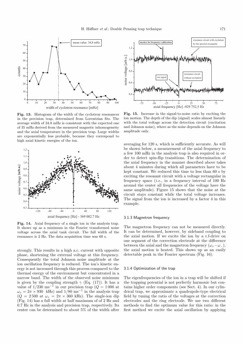
Fig. 13. Histogram of the width of the cyclotron resonancesin the precision trap, determined from Lorentzian fits. Theaverage width of 34.8 mHz is consistent with the expected oneof 35 mHz derived from the measured magnetic inhomogeneityand the axial temperature in the precision trap. Large widthsare exponentially less probable, because they correspond tohigh axial kinetic energies of the ion.
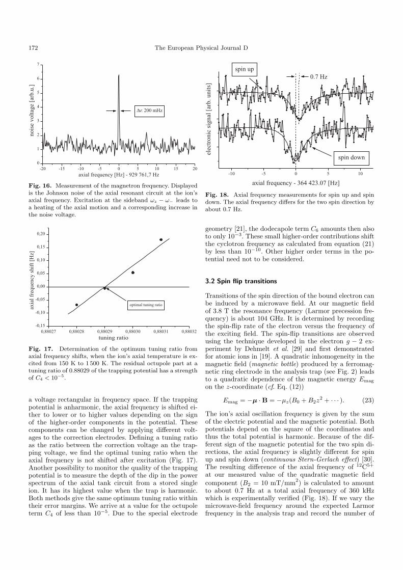
Fig. 14. Axial frequency of a single ion in the analysis trap.It shows up as a minimum in the Fourier transformed noisevoltage across the axial tank circuit. The full width of theresonance is 2 Hz. The data acquisition time was 60 s.
strongly. This results in a high a.c. current with oppositephase, shortening the external voltage at this frequency.Consequently the total Johnson noise amplitude at theion oscillation frequency is reduced. The ion’s kinetic en-ergy is not increased through this process compared to thethermal energy of the environment but concentrated in anarrow band. The width of the observed noise minimumis given by the coupling strength γ (Eq. (17)). It has avalue of 1/230 ms−1 in our precision trap (Q = 1 000 atωz = 2π × 930 kHz) and 1/80 ms−1 in the analysis trap(Q = 2 500 at ωz = 2π × 360 kHz). The single-ion dip(Fig. 14) has a full width at half maximum of of 2 Hz and0.7 Hz in the analysis and precision trap, respectively. Itscenter can be determined to about 5% of the width after
Fig. 15. Increase in the signal-to-noise ratio by exciting theion motion. The depth of the dip (signal) scales almost linearlywith the total voltage across the detection circuit (excitationand Johnson noise), where as the noise depends on the Johnsonamplitude only.
averaging for 120 s, which is sufficiently accurate. As willbe shown below, a measurement of the axial frequency toa few 100 mHz in the analysis trap is also required in or-der to detect spin-flip transitions. The determination ofthe axial frequency in the manner described above takesabout 4 minutes during which all parameters have to bekept constant. We reduced this time to less than 60 s byexciting the resonant circuit with a voltage rectangular infrequency space (i.e., in a frequency interval of 100 Hzaround the center all frequencies of the voltage have thesame amplitude). Figure 15 shows that the noise at thecircuit stays constant while the total voltage increases.The signal from the ion is increased by a factor 4 in thisexample.
3.1.3 Magnetron frequency
The magnetron frequency can not be measured directly.It can be determined, however, by sideband coupling tothe axial motion. If we excite the ion by a r.f-drive onone segment of the correction electrode at the differencebetween the axial and the magnetron frequency (ωz−ω−),the axial motion is heated. This shows up as an easilydetectable peak in the Fourier spectrum (Fig. 16).
3.1.4 Optimization of the trap
The eigenfrequencies of the ion in a trap will be shifted ifthe trapping potential is not perfectly harmonic but con-tains higher order components (see Sect. 4). In our cylin-drical trap, we approximate a quadrupole-type electricalfield by tuning the ratio of the voltages at the correctionelectrodes and the ring electrode. We use two differentmethods to find the optimum value for this ratio: in thefirst method we excite the axial oscillation by applying
172 The European Physical Journal D
Fig. 16. Measurement of the magnetron frequency. Displayedis the Johnson noise of the axial resonant circuit at the ion’saxial frequency. Excitation at the sideband ωz − ω− leads toa heating of the axial motion and a corresponding increase inthe noise voltage.
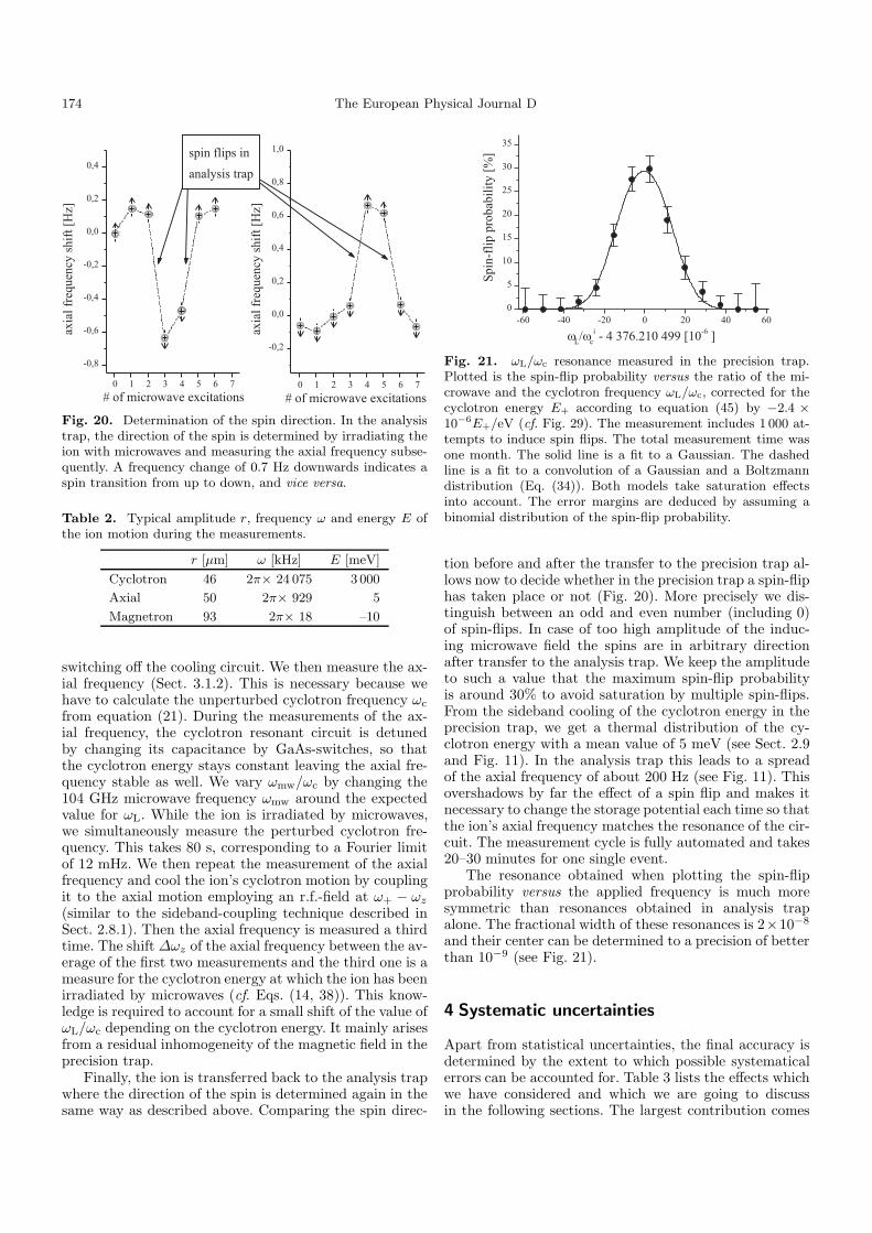
Fig. 17. Determination of the optimum tuning ratio fromaxial frequency shifts, when the ion’s axial temperature is ex-cited from 150 K to 1 500 K. The residual octupole part at atuning ratio of 0.88029 of the trapping potential has a strengthof C4 < 10−5.
a voltage rectangular in frequency space. If the trappingpotential is anharmonic, the axial frequency is shifted ei-ther to lower or to higher values depending on the signof the higher-order components in the potential. Thesecomponents can be changed by applying different volt-ages to the correction electrodes. Defining a tuning ratioas the ratio between the correction voltage an the trap-ping voltage, we find the optimal tuning ratio when theaxial frequency is not shifted after excitation (Fig. 17).Another possibility to monitor the quality of the trappingpotential is to measure the depth of the dip in the powerspectrum of the axial tank circuit from a stored singleion. It has its highest value when the trap is harmonic.Both methods give the same optimum tuning ratio withintheir error margins. We arrive at a value for the octupoleterm C4 of less than 10−5. Due to the special electrode
Fig. 18. Axial frequency measurements for spin up and spindown. The axial frequency differs for the two spin direction byabout 0.7 Hz.
geometry [21], the dodecapole term C6 amounts then alsoto only 10−3. These small higher-order contributions shiftthe cyclotron frequency as calculated from equation (21)by less than 10−10. Other higher order terms in the po-tential need not to be considered.
3.2 Spin flip transitions
Transitions of the spin direction of the bound electron canbe induced by a microwave field. At our magnetic fieldof 3.8 T the resonance frequency (Larmor precession fre-quency) is about 104 GHz. It is determined by recordingthe spin-flip rate of the electron versus the frequency ofthe exciting field. The spin-flip transitions are observedusing the technique developed in the electron g − 2 ex-periment by Dehmelt et al. [29] and first demonstratedfor atomic ions in [19]. A quadratic inhomogeneity in themagnetic field (magnetic bottle) produced by a ferromag-netic ring electrode in the analysis trap (see Fig. 2) leadsto a quadratic dependence of the magnetic energy Emag
on the z-coordinate (cf. Eq. (12))
Emag = −µ · B = −µz(B0 + B2z2 + · · · ). (23)
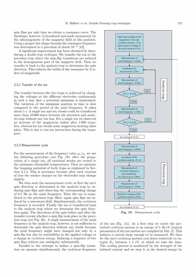
The ion’s axial oscillation frequency is given by the sumof the electric potential and the magnetic potential. Bothpotentials depend on the square of the coordinates andthus the total potential is harmonic. Because of the dif-ferent sign of the magnetic potential for the two spin di-rections, the axial frequency is slightly different for spinup and spin down (continuous Stern-Gerlach effect) [30].The resulting difference of the axial frequency of 12C5+
at our measured value of the quadratic magnetic fieldcomponent (B2 = 10 mT/mm2) is calculated to amountto about 0.7 Hz at a total axial frequency of 360 kHzwhich is experimentally verified (Fig. 18). If we vary themicrowave-field frequency around the expected Larmorfrequency in the analysis trap and record the number of
H. Haffner et al.: Double Penning trap technique 173
spin flips per unit time we obtain a resonance curve. Thelineshape, however, is broadened and made asymmetric bythe inhomogeneity of the magnetic field at this position.Using a proper line shape formula the resonance frequencywas determined to a precision of about 10−6 [19].
A significant improvement has been obtained by intro-ducing a double-trap technique. We transfer the ion to theprecision trap where the spin-flip transitions are inducedin the homogeneous part of the magnetic field. Then wetransfer it back to the analysis trap to determine the spindirection. This reduces the width of the resonance by 3 or-ders of magnitude.
3.2.1 Transfer of the ion
The transfer between the two traps is achieved by chang-ing the voltages at the different electrodes continuouslyin such a way that a potential minimum is maintained.The variation of the minimum position in time is slowcompared to the period of the axial frequency. It takesabout 1 s. A single ion and ion clouds could be transferredmore than 10 000 times between the precision and analy-sis trap without any ion loss. For a single ion we observedno increase of the magnetron radius after 1 000 trans-fers, whereas for ion clouds some magnetron heating takesplace. This is due to ion-ion interaction during the trans-port.
3.2.2 Measurement cycle
For the measurement of the frequency ratio ωL/ωc we usethe following procedure (see Fig. 19): after the prepa-ration of a single ion, all motional modes are cooled tothe minimum obtainable temperatures. Then we optimizethe trapping potential of both traps as explained in Sec-tion 3.1.4. This is necessary because after each creationof ions the surface charges on the electrodes may changeslightly.
We then start the measurement cycle: at first the ion’sspin direction is determined in the analysis trap by in-ducing spin flips and observing the corresponding changeof 0.7 Hz in the axial frequency. Then the ion is trans-ferred to the precision trap. Here, again spin flips are in-duced by a microwave field. Simultaneously, the cyclotronfrequency is recorded. Finally the ion is transferred backto the analysis trap where we determine the spin direc-tion again. The directions of the spin before and after thetransfer reveals whether a spin flip took place in the preci-sion trap (see Fig. 20). A single measurement of the axialfrequency in the analysis trap, however, is not sufficient todetermine the spin direction without any doubt becausethe axial frequency might have changed not only by aspin flip but also by instabilities in the applied voltage ora change in cyclotron energy. Inducing a sequence of twospin flips reduces any ambiguity substantially.
Parallel to the attempt to induce a spin-flip transi-tion we measure simultaneously the cyclotron frequency
Fig. 19. Measurement cycle.
of the ion (Eq. (4)). As a first step we excite the per-turbed cyclotron motion to an energy of 5–20 eV (typicalparameters of the ion motion are compiled in Tab. 2). Thisinduces a current large enough to be measured. We thenlet the ion’s cyclotron motion cool down resistively to en-ergies E+ between 1–5 eV, at which we take the data.The cooling process is monitored by the strength of theinduced current and we stop it at the desired energy by
174 The European Physical Journal D
Fig. 20. Determination of the spin direction. In the analysistrap, the direction of the spin is determined by irradiating theion with microwaves and measuring the axial frequency subse-quently. A frequency change of 0.7 Hz downwards indicates aspin transition from up to down, and vice versa.
Table 2. Typical amplitude r, frequency ω and energy E ofthe ion motion during the measurements.
r [µm] ω [kHz] E [meV]
Cyclotron 46 2π× 24 075 3 000
Axial 50 2π× 929 5
Magnetron 93 2π× 18 –10
switching off the cooling circuit. We then measure the ax-ial frequency (Sect. 3.1.2). This is necessary because wehave to calculate the unperturbed cyclotron frequency ωc
from equation (21). During the measurements of the ax-ial frequency, the cyclotron resonant circuit is detunedby changing its capacitance by GaAs-switches, so thatthe cyclotron energy stays constant leaving the axial fre-quency stable as well. We vary ωmw/ωc by changing the104 GHz microwave frequency ωmw around the expectedvalue for ωL. While the ion is irradiated by microwaves,we simultaneously measure the perturbed cyclotron fre-quency. This takes 80 s, corresponding to a Fourier limitof 12 mHz. We then repeat the measurement of the axialfrequency and cool the ion’s cyclotron motion by couplingit to the axial motion employing an r.f.-field at ω+ − ωz
(similar to the sideband-coupling technique described inSect. 2.8.1). Then the axial frequency is measured a thirdtime. The shift ∆ωz of the axial frequency between the av-erage of the first two measurements and the third one is ameasure for the cyclotron energy at which the ion has beenirradiated by microwaves (cf. Eqs. (14, 38)). This know-ledge is required to account for a small shift of the value ofωL/ωc depending on the cyclotron energy. It mainly arisesfrom a residual inhomogeneity of the magnetic field in theprecision trap.
Finally, the ion is transferred back to the analysis trapwhere the direction of the spin is determined again in thesame way as described above. Comparing the spin direc-
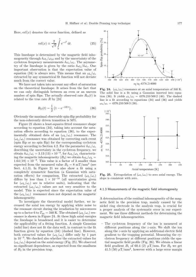
Fig. 21. ωL/ωc resonance measured in the precision trap.Plotted is the spin-flip probability versus the ratio of the mi-crowave and the cyclotron frequency ωL/ωc, corrected for thecyclotron energy E+ according to equation (45) by −2.4 ×10⁻⁶E+/eV (cf. Fig. 29). The measurement includes 1 000 at-tempts to induce spin flips. The total measurement time wasone month. The solid line is a fit to a Gaussian. The dashedline is a fit to a convolution of a Gaussian and a Boltzmanndistribution (Eq. (34)). Both models take saturation effectsinto account. The error margins are deduced by assuming abinomial distribution of the spin-flip probability.
tion before and after the transfer to the precision trap al-lows now to decide whether in the precision trap a spin-fliphas taken place or not (Fig. 20). More precisely we dis-tinguish between an odd and even number (including 0)of spin-flips. In case of too high amplitude of the induc-ing microwave field the spins are in arbitrary directionafter transfer to the analysis trap. We keep the amplitudeto such a value that the maximum spin-flip probabilityis around 30% to avoid saturation by multiple spin-flips.From the sideband cooling of the cyclotron energy in theprecision trap, we get a thermal distribution of the cy-clotron energy with a mean value of 5 meV (see Sect. 2.9and Fig. 11). In the analysis trap this leads to a spreadof the axial frequency of about 200 Hz (see Fig. 11). Thisovershadows by far the effect of a spin flip and makes itnecessary to change the storage potential each time so thatthe ion’s axial frequency matches the resonance of the cir-cuit. The measurement cycle is fully automated and takes20–30 minutes for one single event.
The resonance obtained when plotting the spin-flipprobability versus the applied frequency is much moresymmetric than resonances obtained in analysis trapalone. The fractional width of these resonances is 2×10⁻⁸
and their center can be determined to a precision of betterthan 10−9 (see Fig. 21).
4 Systematic uncertainties
Apart from statistical uncertainties, the final accuracy isdetermined by the extent to which possible systematicalerrors can be accounted for. Table 3 lists the effects whichwe have considered and which we are going to discussin the following sections. The largest contribution comes
H. Haffner et al.: Double Penning trap technique 175
Table 3. Systematic uncertainties of ωL/ωc which are consid-ered. The corresponding sections are indicated in parentheses.All uncertainties are given in relative units.
asymmetry of resonance (4.1.2) 2 × 10⁻¹⁰
measurement of cyclotron energy (4.2) 2 × 10⁻¹⁰
electric field imperfections (4.4) 1 × 10⁻¹⁰
cavity-QED shifts (4.5) ≈ 10−13
interaction with image charges (4.5) 3 × 10⁻¹¹
relativistic corrections (4.6) 1 × 10⁻¹²
magnetron energy (4.7) 1 × 10⁻¹¹
shift by standing microwave field (4.7) < 10−14
stability of quartz oscillators (4.7) 1 × 10⁻¹⁰
grounding of apparatus (4.7) 4 × 10⁻¹¹
saturation of spin-flip transition 5 × 10⁻¹²
spectral purity of microwaves 5 × 10⁻¹³
damping of ion motion ≈ 10−20
total (quadrature sum) 3 × 10⁻¹⁰
Table 4. Corrections which are included in the final evalua-tion of the experimental value for ωL/ωc.
experimental value 4376.210 500 2
interaction with image charges (4.5) −0.000 001 2
shift due to grounding (4.7) −0.000 000 3
cyclotron energy measurement (4.2) +0.000 000 3
final experimental value 4376.210 499 0
from our understanding of the resonance line shape whichis affected by a small residual inhomogeneity of the mag-netic field in the precision trap. We are also going to dis-cuss some corrections that we have to apply to our finalexperimental value (see Tab. 4).
4.1 Lineshape
4.1.1 Basic lineshapes
In a perfectly homogeneous magnetic field, the cy-clotron and Larmor resonances would be described by aLorentzian lineshape. The slight inhomogeneity of the fieldin the precision trap caused by the residual influence ofthe nickel ring in the analysis trap, 27 mm apart, leads todistortions. The shape of both resonances in an inhomo-geneous magnetic field of the form given by equation (12)was calculated by Brown [31,32].
In our experiment for each test of a certain ratioof ωmw/ωc, the influence of the cyclotron energy can beneglected because the ion is decoupled from the environ-ment during the measurement. The axial mode, however,is strongly coupled to the resonant circuit with a time con-stant of 1/γ = 233 ms. The basic broadening process isthe dependence of the average field on the thermally fluc-tuating axial energy (Eqs. (15, 16)). For this reason, theaxial energy distribution should show up in the lineshape.
∆ν
0,1 0,2 0,3 0,4
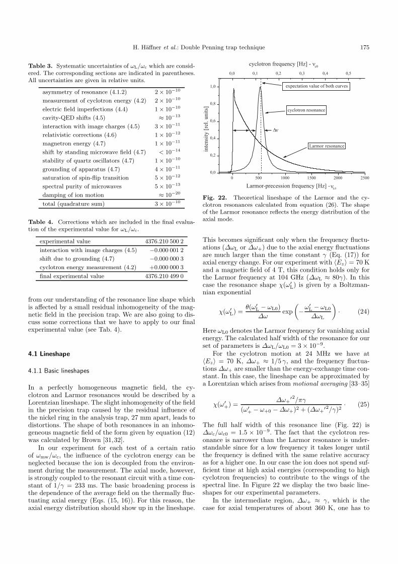
Fig. 22. Theoretical lineshape of the Larmor and the cy-clotron resonances calculated from equation (26). The shapeof the Larmor resonance reflects the energy distribution of theaxial mode.
This becomes significant only when the frequency fluctu-ations (∆ωL or ∆ω+) due to the axial energy fluctuationsare much larger than the time constant γ (Eq. (17)) foraxial energy change. For our experiment with 〈Ez〉 = 70 Kand a magnetic field of 4 T, this condition holds only forthe Larmor frequency at 104 GHz (∆ωL ≈ 80γ). In thiscase the resonance shape χ(ω′
L) is given by a Boltzman-nian exponential
χ(ω′L) =
θ(ω′L − ωL0)∆ω
exp(−ω′
L − ωL0
∆ωL
)· (24)
Here ωL0 denotes the Larmor frequency for vanishing axialenergy. The calculated half width of the resonance for ourset of parameters is ∆ωL/ωL0 = 3 × 10⁻⁹.
For the cyclotron motion at 24 MHz we have at〈Ez〉 = 70 K, ∆ω+ ≈ 1/5 γ, and the frequency fluctua-tions ∆ω+ are smaller than the energy-exchange time con-stant. In this case, the lineshape can be approximated bya Lorentzian which arises from motional averaging [33–35]
χ(ω′+) =
∆ω+′2/πγ
(ω′+ − ω+0 − ∆ω+)2 + (∆ω+
′2/γ)2· (25)
The full half width of this resonance line (Fig. 22) is∆ωc/ωc0 = 1.5 × 10⁻⁹. The fact that the cyclotron res-onance is narrower than the Larmor resonance is under-standable since for a low frequency it takes longer untilthe frequency is defined with the same relative accuracyas for a higher one. In our case the ion does not spend suf-ficient time at high axial energies (corresponding to highcyclotron frequencies) to contribute to the wings of thespectral line. In Figure 22 we display the two basic line-shapes for our experimental parameters.
In the intermediate region, ∆ω+ ≈ γ, which is thecase for axial temperatures of about 360 K, one has to
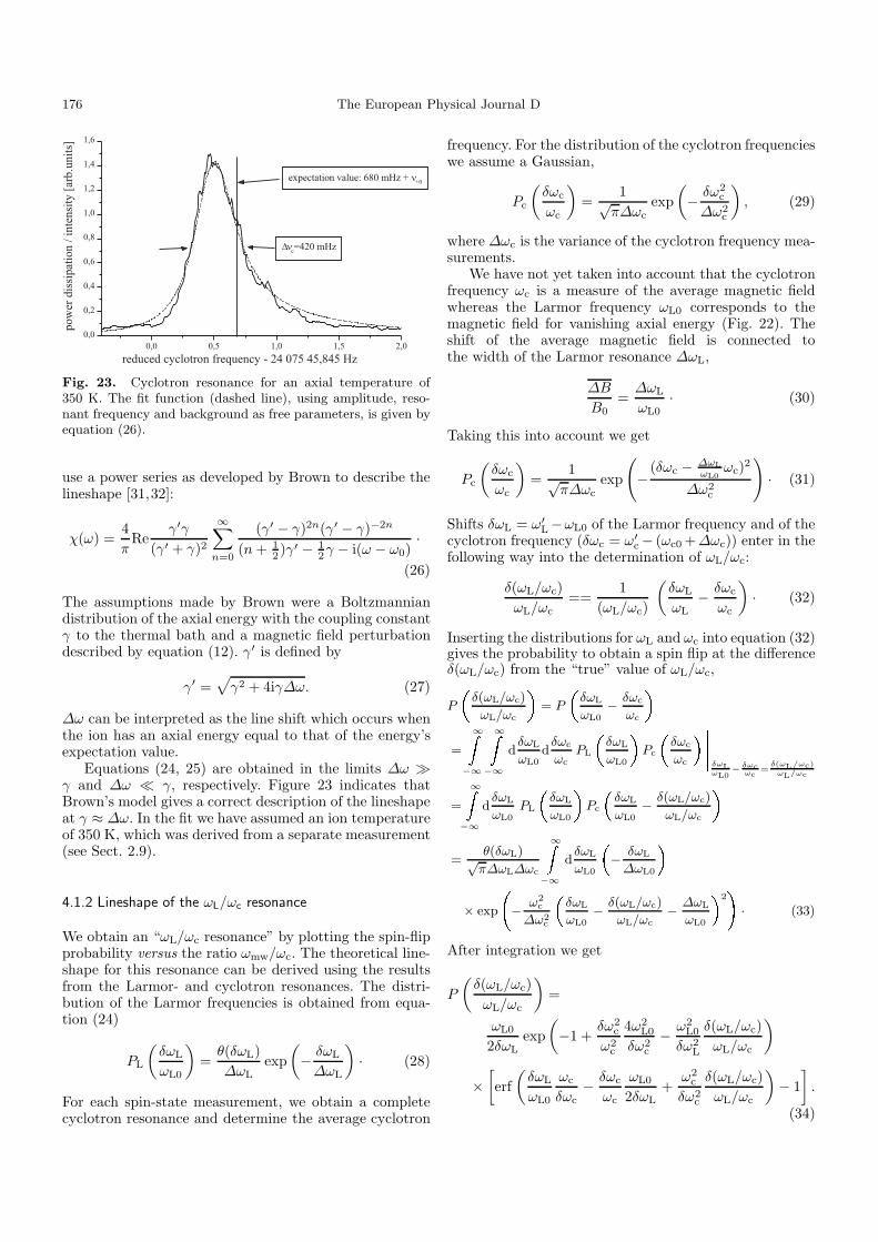
176 The European Physical Journal D
Fig. 23. Cyclotron resonance for an axial temperature of350 K. The fit function (dashed line), using amplitude, reso-nant frequency and background as free parameters, is given byequation (26).
use a power series as developed by Brown to describe thelineshape [31,32]:
χ(ω) =4π
Reγ′γ
(γ′ + γ)2
∞∑n=0
(γ′ − γ)2n(γ′ − γ)−2n
(n + 12 )γ′ − 1
2γ − i(ω − ω0)·
(26)
The assumptions made by Brown were a Boltzmanniandistribution of the axial energy with the coupling constantγ to the thermal bath and a magnetic field perturbationdescribed by equation (12). γ′ is defined by
γ′ =√
γ2 + 4iγ∆ω. (27)
∆ω can be interpreted as the line shift which occurs whenthe ion has an axial energy equal to that of the energy’sexpectation value.
Equations (24, 25) are obtained in the limits ∆ω γ and ∆ω γ, respectively. Figure 23 indicates thatBrown’s model gives a correct description of the lineshapeat γ ≈ ∆ω. In the fit we have assumed an ion temperatureof 350 K, which was derived from a separate measurement(see Sect. 2.9).
4.1.2 Lineshape of the ωL/ωc resonance
We obtain an “ωL/ωc resonance” by plotting the spin-flipprobability versus the ratio ωmw/ωc. The theoretical line-shape for this resonance can be derived using the resultsfrom the Larmor- and cyclotron resonances. The distri-bution of the Larmor frequencies is obtained from equa-tion (24)
PL
(δωL
ωL0
)=
θ(δωL)∆ωL
exp(− δωL
∆ωL
)· (28)
For each spin-state measurement, we obtain a completecyclotron resonance and determine the average cyclotron
frequency. For the distribution of the cyclotron frequencieswe assume a Gaussian,
Pc
(δωc
ωc
)=
1√π∆ωc
exp(− δω2
c
∆ω2c
), (29)
where ∆ωc is the variance of the cyclotron frequency mea-surements.
We have not yet taken into account that the cyclotronfrequency ωc is a measure of the average magnetic fieldwhereas the Larmor frequency ωL0 corresponds to themagnetic field for vanishing axial energy (Fig. 22). Theshift of the average magnetic field is connected tothe width of the Larmor resonance ∆ωL,
∆B
B0=
∆ωL
ωL0· (30)
Taking this into account we get
Pc
(δωc
ωc
)=
1√π∆ωc
exp
(− (δωc − ∆ωL
ωL0ωc)2
∆ω2c
)· (31)
Shifts δωL = ω′L −ωL0 of the Larmor frequency and of the
cyclotron frequency (δωc = ω′c − (ωc0 +∆ωc)) enter in the
following way into the determination of ωL/ωc:
δ(ωL/ωc)ωL/ωc
==1
(ωL/ωc)
(δωL
ωL− δωc
ωc
)· (32)
Inserting the distributions for ωL and ωc into equation (32)gives the probability to obtain a spin flip at the differenceδ(ωL/ωc) from the “true” value of ωL/ωc,
P
δ(ωL/ωc)
ωL/ωc
= P
δωL
ωL0− δωc
ωc
=
∞−∞
∞−∞
dδωL
ωL0d
δωc
ωcPL
δωL
ωL0
Pc
δωc
ωc
δωLωL0
− δωcωc
=δ(ωL/ωc)
ωL/ωc
=
∞−∞
dδωL
ωL0PL
δωL
ωL0
Pc
δωL
ωL0− δ(ωL/ωc)
ωL/ωc
=θ(δωL)√
π∆ωL∆ωc
∞−∞
dδωL
ωL0
− δωL
∆ωL0
× exp
− ω2
c
∆ω2c
δωL
ωL0− δ(ωL/ωc)
ωL/ωc− ∆ωL
ωL0
2
· (33)
After integration we get
P
(δ(ωL/ωc)ωL/ωc
)=
ωL0
2δωLexp
(−1 +
δω2c
ω2c
4ω2L0
δω2c
− ω2L0
δω2L
δ(ωL/ωc)ωL/ωc
)
×[erf(
δωL
ωL0
ωc
δωc− δωc
ωc
ωL0
2δωL+
ω2c
δω2c
δ(ωL/ωc)ωL/ωc
)− 1]
.
(34)
H. Haffner et al.: Double Penning trap technique 177
Here, erf(x) denotes the error function, defined as
erf(x) ≡ 2√π
x∫0
e−t2 dt. (35)
This lineshape is determined by the magnetic field inho-mogeneity through δωL/ωL0 and by the uncertainty of thecyclotron frequency measurements δωc/ωc. The asymme-try of the lineshape is given by the ratio δωL/δωc. Oneimportant observation is that the expectation value ofequation (34) is always zero. This means that an ωL/ωc
extracted by any symmetrical fit function will not deviatemuch from the correct value.
We have not taken into account any effect of saturationon the theoretical lineshape. It arises from the fact thatwe can only distinguish between an even or an unevennumber of spin flips. The actually observed rate RO(t) isrelated to the true rate R by [24]
RO(t) =12(1 − e−2R t
). (36)
Obviously the maximal observable spin-flip probability forthe non-coherently driven transition is 50%.
Figure 21 shows a least-squares fitted resonance shapeaccording to equation (34), taking into account the satu-ration effects according to equation (36), to the exper-imentally obtained data of an (ωL/ωc) resonance. The(ωL/ωc) resonance was obtained by correcting each event(spin flip or no spin flip) for the corresponding cyclotronenergy according to Section 4.2. For the parameter δωc/ωc
describing the uncertainty in the cyclotron frequency, weobtain δωc/ωc = 3.13 (13)×10−9, for δωL/ωL characteriz-ing the magnetic inhomogeneity (B2) we obtain δωL/ωL =1.64 (18) × 10−9. This value is a factor of 3 smaller thanexpected from the measured value B2 = 8 mT/mm2 (seeSect. 4.1.3). In Figure 21 we also show a fit using acompletely symmetric function (a Gaussian with satu-ration effects) for comparison. The extracted (ωL/ωc)differs by less than 1 × 10⁻¹⁰ (all uncertainties givenfor (ωL/ωc) are in relative units), indicating that theextracted (ωL/ωc) values are not very sensitive to themodel. This is expected since the expectation value ofthe (ωL/ωc) resonance does not depend on the magneticinhomogeneity.
To investigate the theoretical model further, we in-creased the axial ion energy by applying white noise tothe resonant circuit during the irradiation by microwavesup to a factor 6 to Tax = 340 K. The obtained (ωL/ωc) res-onance is shown in Figure 24. At these high axial energiesthe lineshape is broadened and it is easier to determinethe applicability of a fitting function. A simple Gaussian(solid line) does not fit the data well, in contrast to the fitfunction given by equation (34) (dashed line). However,both extracted values for (ωL/ωc) differ only by 1 partin 10−9. We checked also whether the extracted values for(ωL/ωc) depend on the axial energy (Fig. 25). We observedno significant dependence, as expected from the smallnessof B2 in the precision trap.
Fig. 24. (ωL/ωc) resonance at an axial temperature of 340 K.The solid line is a fit using a Gaussian inserted into equa-tion (36). It yields ωL/ωc = 4376.210 500 2 (46). The dashedline is a fit according to equations (34) and (36) and yieldsωL/ωc = 4376.210 508 3 (38).
Fig. 25. Extrapolation of (ωL/ωc) to zero axial energy. Theslope is consistent with zero.
4.1.3 Measurements of the magnetic field inhomogeneity
A determination of the residual inhomogeneity of the mag-netic field in the precision trap, mainly caused by thenickel ring electrode in the analysis trap, is crucial fora proper analysis of the systematic error in our experi-ment. We use three different methods for determining themagnetic field inhomogeneities.
– The cyclotron frequency of the ion is measured atdifferent positions along the z-axis. We shift the ionalong the z-axis by applying an additional electric fieldgradient to the trapping potential. Measuring the cy-clotron frequency at different positions yields the spa-tial magnetic field profile (Fig. 26). We obtain a linearfield gradient B1 of 60.4 (2) µT/mm. For B2 we get41.5 (50) µT/mm2, however with a large error margin
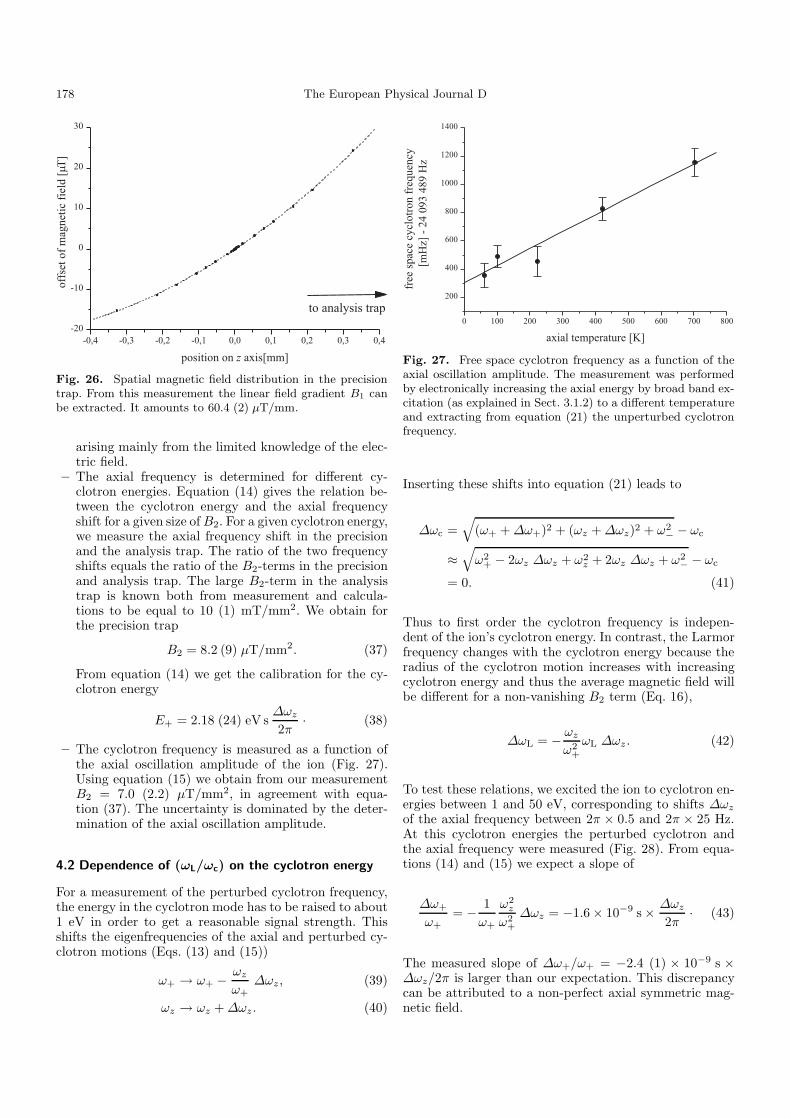
178 The European Physical Journal D
Fig. 26. Spatial magnetic field distribution in the precisiontrap. From this measurement the linear field gradient B1 canbe extracted. It amounts to 60.4 (2) µT/mm.
arising mainly from the limited knowledge of the elec-tric field.
– The axial frequency is determined for different cy-clotron energies. Equation (14) gives the relation be-tween the cyclotron energy and the axial frequencyshift for a given size of B2. For a given cyclotron energy,we measure the axial frequency shift in the precisionand the analysis trap. The ratio of the two frequencyshifts equals the ratio of the B2-terms in the precisionand analysis trap. The large B2-term in the analysistrap is known both from measurement and calcula-tions to be equal to 10 (1) mT/mm2. We obtain forthe precision trap
B2 = 8.2 (9) µT/mm2. (37)
From equation (14) we get the calibration for the cy-clotron energy
E+ = 2.18 (24) eV s∆ωz
2π· (38)
– The cyclotron frequency is measured as a function ofthe axial oscillation amplitude of the ion (Fig. 27).Using equation (15) we obtain from our measurementB2 = 7.0 (2.2) µT/mm2, in agreement with equa-tion (37). The uncertainty is dominated by the deter-mination of the axial oscillation amplitude.
4.2 Dependence of (ωL/ωc) on the cyclotron energy
For a measurement of the perturbed cyclotron frequency,the energy in the cyclotron mode has to be raised to about1 eV in order to get a reasonable signal strength. Thisshifts the eigenfrequencies of the axial and perturbed cy-clotron motions (Eqs. (13) and (15))
ω+ → ω+ − ωz
ω+∆ωz, (39)
ωz → ωz + ∆ωz. (40)
Fig. 27. Free space cyclotron frequency as a function of theaxial oscillation amplitude. The measurement was performedby electronically increasing the axial energy by broad band ex-citation (as explained in Sect. 3.1.2) to a different temperatureand extracting from equation (21) the unperturbed cyclotronfrequency.
Inserting these shifts into equation (21) leads to
∆ωc =√
(ω+ + ∆ω+)2 + (ωz + ∆ωz)2 + ω2− − ωc
≈√
ω2+ − 2ωz ∆ωz + ω2
z + 2ωz ∆ωz + ω2− − ωc
= 0. (41)
Thus to first order the cyclotron frequency is indepen-dent of the ion’s cyclotron energy. In contrast, the Larmorfrequency changes with the cyclotron energy because theradius of the cyclotron motion increases with increasingcyclotron energy and thus the average magnetic field willbe different for a non-vanishing B2 term (Eq. 16),
∆ωL = − ωz
ω2+
ωL ∆ωz. (42)
To test these relations, we excited the ion to cyclotron en-ergies between 1 and 50 eV, corresponding to shifts ∆ωz
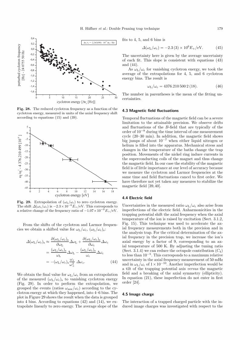
of the axial frequency between 2π × 0.5 and 2π × 25 Hz.At this cyclotron energies the perturbed cyclotron andthe axial frequency were measured (Fig. 28). From equa-tions (14) and (15) we expect a slope of
∆ω+
ω+= − 1
ω+
ω2z
ω2+
∆ωz = −1.6 × 10⁻⁹ s × ∆ωz
2π· (43)
The measured slope of ∆ω+/ω+ = −2.4 (1) × 10−9 s ×∆ωz/2π is larger than our expectation. This discrepancycan be attributed to a non-perfect axial symmetric mag-netic field.
H. Haffner et al.: Double Penning trap technique 179
Fig. 28. The reduced cyclotron frequency as a function of thecyclotron energy, measured in units of the axial frequency shiftaccording to equations (15) and (39).
Fig. 29. Extrapolation of (ωL/ωc) to zero cyclotron energy.The shift ∆(ωL/ωc) is −2.3×10⁻⁶E+/eV. This corresponds toa relative change of the frequency ratio of −1.07×10⁻⁹ E+/eV.
From the shifts of the cyclotron and Larmor frequen-cies we obtain a shifted value for ωL/ωc, (ωL/ωc)s:
∆(ωL/ωc)s ≈ ∂(ωL/ωc)s∂ωL
∆ωL +∂(ωL/ωc)s
∂ωc∆ωc
=(ωL/ωc)s
ωL∆ωL − (ωL/ωc)s
ωc∆ωc
= −(ωL/ωc)sωz
ω2+
∆ωz. (44)
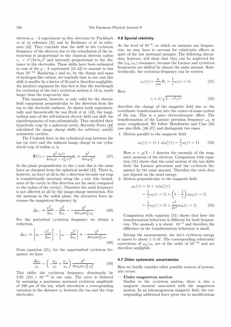
We obtain the final value for ωL/ωc from an extrapolationof the measured (ωL/ωc)s to vanishing cyclotron energy(Fig. 29). In order to perform the extrapolation, wegrouped the events (ratios ωmw/ωc) according to the cy-clotron energy at which they happened, into 4–6 bins. Theplot in Figure 29 shows the result when the data is groupedinto 4 bins. According to equations (42) and (14), we ex-trapolate linearly to zero energy. The average slope of the
fits to 4, 5, and 6 bins is
∆(ωL/ωc) = −2.3 (3)× 106E+/eV. (45)
The uncertainty here is given by the average uncertaintyof each fit. This slope is consistent with equations (43)and (44).
As ωL/ωc for vanishing cyclotron energy, we took theaverage of the extrapolations for 4, 5, and 6 cyclotronenergy bins. The result is
ωL/ωc = 4376.210 500 2 (18). (46)
The number in parentheses is the mean of the fitting un-certainties.
4.3 Magnetic field fluctuations
Temporal fluctuations of the magnetic field can be a severelimitation to the attainable precision. We observe driftsand fluctuations of the B-field that are typically of theorder of 10−8 during the time interval of one measurementcycle (20–30 min). In addition, the magnetic field showsbig jumps of about 10−7 when either liquid nitrogen orhelium is filled into the apparatus. Mechanical stress andchanges in the temperature of the baths change the trapposition. Movements of the nickel ring induce currents inthe superconducting coils of the magnet and thus changethe magnetic field. In our case the stability of the magneticfield is of little importance at our level of accuracy becausewe measure the cyclotron and Larmor frequencies at thesame time and field fluctuations cancel to first order. Wehave therefore not yet taken any measures to stabilize themagnetic field [39,40].
4.4 Electric field
Uncertainties in the measured ratio ωL/ωc also arise fromimperfections of the electric field. Anharmonicities in thetrapping potential shift the axial frequency when the axialtemperature of the ion is raised by excitation (Sect. 3.1.2,Fig. 15). This technique was used to accelerate the ax-ial frequency measurements both in the precision and inthe analysis trap. For the critical determination of the ax-ial frequency in the precision trap, we increase the ion’saxial energy by a factor of 9, corresponding to an ax-ial temperature of 500 K. By adjusting the tuning ratio(Sect. 3.1.4) we can reduce the octupole contribution (C4)to less than 10−5. This corresponds to a maximum relativeuncertainty in the axial frequency measurement of 50 mHzand in ωL/ωc of 1×10⁻¹⁰. Another imperfection would bea tilt of the trapping potential axis versus the magneticfield and a breaking of the axial symmetry (ellipticity).In equation (21), these imperfection do not enter in firstorder [24].
4.5 Image charge
The interaction of a trapped charged particle with the in-duced image charges was investigated with respect to the
180 The European Physical Journal D
electron g − 2 experiment on free electrons by Fischbachet al. in reference [41] and by Boulware et al. in refer-ence [42]. They conclude that the shift in the cyclotronfrequency of the electron due to the retardation of the in-teraction is proportional to the classical electron radiusre = e2/2πmec
2 and inversely proportional to the dis-tance to the electrodes. These shifts have been estimatedin case of the g − 2 experiment [41,42] to amount to lessthan 10−12. Replacing e and me by the charge and massof hydrogen-like carbon, we conclude that in our case thisshift is smaller by a factor of 50 and is therefore negligible.An intuitive argument for this fact is that the wavelengthfor excitation of the ion’s cyclotron motion is 12 m, muchlarger than the trap-cavity size.
This argument, however, is only valid for the electricfield component perpendicular to the direction from theion to the electrode surfaces. As shown both experimen-tally and theoretically by van Dyck et al. [43], the longi-tudinal part of the self-induced electric field can shift theeigenfrequencies of ions substantially. They modeled theirhyperbolic trap by a spherical cavity. Recently Porto [44]calculated the image charge shifts for arbitrary axiallysymmetric cavities.
The Coulomb force in the cylindrical trap between theion (at rest) and the induced image charge in our cylin-drical trap of radius r0 is
F(r) =q2 r0/r
4πε0|r − r20/r|2 er ≈ q2
4πε0r30
r. (47)
In the plane perpendicular to the z-axis this is the sameforce as obtained from the spherical model [43]. There is,however, no force at all in the z-direction because our trapis translationally invariant along the z-axis (the bound-aries of the cavity in this direction are far away comparedto the radius of the cavity). Therefore the axial frequencyis not affected at all by the image-charge interaction. Forthe motions in the radial plane, the attractive force in-creases the magnetron frequency by
∆ω− ≈ ω2z,v
2ωc− ω2
z
2ωc= +
q2
4πε0mr30 ωc
· (48)
For the perturbed cyclotron frequency we obtain areduction,
∆ω+ ≈[ωc −
ω2z,v
2ωc
]−[ωc − ω2
z
2ωc
]≈ − q2
4πε0mr30 ωc
·(49)
From equation (21), for the unperturbed cyclotron fre-quency we have
∆ωc
ωc=(−ω+
ωc+
ω−ωc
)q2
4πε0m r30 ω2
c
· (50)
This shifts the cyclotron frequency downwards by2.92 (24) × 10−10 in our case. The error is deducedby assuming a maximum motional cyclotron amplitudeof 100 µm of the ion, which introduces a correspondingvariation in the distance r0 between the ion and the trapelectrodes.
4.6 Special relativity
At the level of 10−9, to which we measure our frequen-cies, we may have to account for relativistic effects inspite of the low motional energies. The following discus-sion, however, will show that they can be neglected forthe (ωL/ωc) resonance, because the Larmor and cyclotronfrequencies are shifted by almost the same amount. Rela-tivistically, the cyclotron frequency can be written
ωc(γ) =q
γmBz =
1γ
ωc(γ = 1). (51)
Here
γ = 1/√
1 − v2/c2 (52)
describes the change of the magnetic field due to thecoordinate transformation into the center-of-mass systemof the ion. This is a pure electrodynamic effect. Thetransformation of the Larmor precision frequency ωL ismore complicated. We follow Mendlowitz and Case [45](see also Refs. [46,47]) and distinguish two cases.1. Motion parallel to the magnetic field:
ωL(γ) = (1 + a)ωec(γ) =
1γ
ωL(γ = 1). (53)
Here a = g/2 − 1 denotes the anomaly of the mag-netic moment of the electron. Comparison with equa-tion (51) shows that the axial motion of the ion shiftsboth the Larmor precession and the cyclotron fre-quency by the same amount. Therefore the ratio doesnot depend on the axial energy.
2. Motion perpendicular to the magnetic field:
ωL(γ) = (1 + γa)ωec(γ)
=1γ
ωL(γ = 1) +(
1 − 1γ
)aωL(γ = 1)
=1γ
ωL(γ = 1) +v2
2c2aωL(γ = 1). (54)
Comparison with equation (51) shows that here thetransformation behaviour is different for both frequen-cies. The anomaly a is about 10−3 and therefore thedifference in the transformation behaviour is small.
During the measurement, the ion’s cyclotron energyis raised to about 1–5 eV. The corresponding relativisticcorrections of ωL/ωc are of the order of 10−12 and aretherefore negligible.
4.7 Other systematic uncertainties
Here we briefly consider other possible sources of system-atic errors.– Finite magnetron motion
Similar to the cyclotron motion, there is also amagnetic moment associated with the magnetronmotion. In an inhomogeneous magnetic field, the cor-responding additional force gives rise to modifications
H. Haffner et al.: Double Penning trap technique 181
of equation (9). But due to the low frequency, theresulting magnetic moment is very small. Since themagnetron radius is of the same order as the cyclotronradius (see Tab. 2) is orbital magnetic moment issmaller by the ratio of frequencies (10−3). From themeasured dependence an the cyclotron energy wecalculate the relative corrections to ωL/ωc to less10−11 for the magnetron motion.
– Microwave fieldInside of our cavity, the microwave field forms astanding wave with a periodicity of 1.5 mm. Since theion amplitudes are in the range of 100 µm, the inten-sity varies by about 3%. This causes a slightly higherspin-flip probability at positions of high microwaveintensity. Together with the magnetic field gradientof 60 µT/mm (corresponding to relative gradientof 1.5 × 10⁻⁶) this would lead to a systematic shiftfor ωL/ωc of 0.03 × 1.5 × 10−6 ≈ 5 × 10⁻⁸. However,the spin-flip rate is much smaller than the oscillationfrequencies so that the spin flips occur on a timescale long compared to the oscillation periods andthus the effect of the inhomogeneous microwave fieldis strongly reduced. Because of the geometry of themicrowave field, we would expect the largest effectfrom the axial motion, which can be estimated to beless than 10−14, assuming a coherence time of 1 s(which actually might even be substantially longerand thus reducing the effect even more).
– Quartz oscillatorsFor the experiment, all synthesizers were locked in achain to a 10 MHz signal of an atomic clock. However,it was not possible to lock our Fast-Fourier-transform(FFT) analyzer which measures the cyclotron fre-quency mixed down from 24 MHz to 1.5 kHz.Therefore we corrected the FFT data for the mea-sured deviation of its oscillator from the clock signal.Assuming a (moderate) stability of 2 × 10⁻⁶ of theFFT oscillator we obtain a final relative contributionof 1 × 10⁻¹⁰ to the uncertainty in ωL/ωc.
– GroundingA small correction also arises from an observed changein the grounding potential when we measure the ax-ial and the cyclotron frequency. The change of theground of about 1 µV is induced by control commandssent by the computer over the GPIB-interface. Theaxial frequency is shifted during its measurement byabout 50 mHz as compared to its value while thecyclotron frequency measurement takes place. Thefractional shift for ωc from equation (21) and corre-sponding for ωL/ωc is 7 × 10⁻¹¹. The uncertainty isconservatively estimated to 4 × 10⁻⁴. This leads to afractional shift of 7×10⁻¹¹ for ωc in and therefore alsofor ωL/ωc.
5 Final result
The quantity measured in our experiment is the ratio ofthe Larmor frequency of the electron bound in 12C5+ and
the cyclotron frequency of the 12C5+-ion. The result afterall corrections (Tab. 4) and extrapolations (Sects. 4.2 and4.1.2) is
ωL/ωc(C5+) = 4 376.210 498 9 (19) (13). (55)
The first number in parentheses refers to the statisticaluncertainty resulting from the extrapolations and the sec-ond one represents the quadratically summed systematicuncertainties (see Tab. 3).
Applying the ratio of cyclotron frequencies for theelectron and 12C5+ (Eq. (5)) derived from measure-ments by van Dyck et al. [17,18] (6me/M12C6+ =0.000 274 365 185 89) (58) and using equation (4), we ob-tain the gJ factor of the electron bound in 12C5+
g(C5+) = 2.001 041 596 (5). (56)
This is the most precise determination of any atomicmagnetic moment so far. It also accurately quantifies forthe first time experimentally the effects of bound-stateQED on a magnetic moment. Our result is in good agree-ment with the theoretical calculations from the groups inSt. Petersburg [15,48] and Goteborg [2,49] and verifiesthe bound-state-QED contributions to about 1%. As wasshown in [14], it even allows for an independent determi-nation of the mass of the electron.
Future prospects
Currently the accuracy to which ωL/ωc can be determinedis limited mainly by magnetic field inhomogeneities. Theylead both to systematic and statistical uncertainties. Themain part of the systematic uncertainty is the asymmetryin the lineshape (Sect. 4.1.2) and the energy dependenceof the cyclotron frequency (Sect. 4.2). The statistical un-certainty is mainly determined by the number of observedspin flips and the width of the line. All of the uncertain-ties caused by the magnetic inhomogeneity add to themost significant contributions of the total error budget.Therefore we plan to improve the spatial homogeneity bytuning the currents in the shim coils of the magnet. Thetuning can be monitored by the methods described in Sec-tion 4.1.3. It should be possible to reduce the quadraticpart of the B-field, characterized by B2, by about a factorof 10 compared to its present value. As a consequence, theresonance would be narrower and the remaining asymme-try would be smaller. Recently we have stabilized the he-lium pressures in the magnet and apparatus dewars. Theconstant pressure reduces temperature fluctuations in thecoil material and thus leads to a more stable flux densityof the magnetic field [40,50].
It is of equal importance to reduce the axial tempera-ture from 60 K to that of the environment at 4 K. The cor-responding reduction in motional amplitude would lead toa smaller linewidth, too. It is, however, difficult to locatethe source of additional noise since our electronic circuitsare not accessible while operating at 4 K.
After improving the homogeneity of the magnetic field,the remaining statistical uncertainty would be dominated
182 The European Physical Journal D
by axial-frequency fluctuations. Here the limitation is notthe statistical noise in the measurement signal, but theelectric field fluctuations in the µV-range. These could bereduced by improving the stability of our voltage source.
We point out that our method to determine the g fac-tor of the bound electron can be applied to almost anyatomic system without reduction in the expected accuracyprovided masses are known well enough. For hydrogen likeions with higher nuclear charge the axial frequency changeconnected with a spin-flip will be smaller. This has to becompensated by a larger magnetic field inhomogeneity inthe analysis trap to make this change observable [51]. Evenmeasurements of the proton and of nuclear magnetic mo-ments are imaginable [52]. Extension of our measurementsto other ions requires a precise knowledge of their atomicmasses (or the ratio of the electron and the ion cyclotronfrequencies). For many ions such accurate mass measure-ments (∆m/m ∼ 10−10) have already been carried out[17,53,54] and thus are a promising base for future exper-iments at our setup.
We are grateful to G. Soff, V.A. Yerokhin, V.M. Shabaev,V. Natarajan, S. Peil, and J.V. Porto, for many stimulatingand helpful discussions. Financial support was obtained fromthe European Union under the contract numbers ERB FMRXCT 97-0144 (EUROTRAPS project) and HPRI-CT-2001-5036(HITRAP project).
References
1. W. Quint, Phys. Scripta T59, 203 (1995)2. T. Beier et al., Phys. Rev. A 62, 032510 (2000)3. H. Haffner et al., Phys. Rev. Lett. 85, 5308 (2000)4. P. Mohr, G. Plunien, G. Soff, Phys. Rep. 293, 227 (1998)5. T. Beier, Phys. Rep. 339, 79 (2000)6. V.M. Shabaev et al., Phys. Rev. Lett. 86, 3959 (2001)7. L.C. Balling, F.M. Pipkin, Phys. Rev. 139, A19 (1965)8. F.G. Walther, W.D. Phillips, D. Kleppner, Phys. Rev.
Lett. 28, 1159 (1972)9. J.S. Tiedeman, H.G. Robinson, Phys. Rev. Lett. 39, 602
(1977)10. C.E. Johnson, H.G. Robinson, Phys. Rev. Lett. 45, 250
(1980)11. P. Seelig et al., Phys. Rev. Lett. 81, 4824 (1998)12. H. Winter et al., GSI Scientific Report 1998, p. 87, 199913. V.M. Shabaev, Can. J. Phys. 76, 907 (1998)14. T. Beier et al., Phys. Rev. Lett. 88, 011603 (2002)15. V.A. Yerokhin, P. Indelicato, V.M. Shabaev, Phys. Rev.
Lett. 89, 143001 (2002)16. P.J. Mohr, B.N. Taylor, Rev. Mod. Phys. 72, 351 (2000)17. R.S. van Dyck Jr, D.L. Farnham, P.B. Schwinberg, Phys.
Scripta T59, 134 (1995)18. D.L. Farnham, R.S. van Dyck Jr, P.B. Schwinberg, Phys.
Rev. Lett. 75, 3598 (1995)19. N. Hermanspahn et al., Phys. Rev. Lett. 84, 427 (2000)20. M. Diederich et al., Hyper. Interact. 115, 185 (1998)21. G. Gabrielse, L. Haarsma, S.L. Rolston, Int. J. Mass Spec-
trom. Ion Process. 88, 319 (1989)
22. R.E. Olson, A. Salop, Phys. Rev. A 14, 579 (1976)23. S. Stahl, Ph.D. thesis, University of Mainz, Germany, 199824. L.S. Brown, G. Gabrielse, Rev. Mod. Phys. 58, 233 (1986)25. L.S. Brown, G. Gabrielse, Phys. Rev. A 25, 2423 (1982)26. D.J. Wineland, H.G. Dehmelt, J. Appl. Phys. 46, 919
(1975)27. E.A. Cornell, R.M. Weisskoff, K.R. Boyce, D.E. Pritchard,
Phys. Rev. A 41, 312 (1990)28. M. Kretzschmar, in Trapped Charged Particles and Fun-
damental Physics, edited by D. Dubin, D. Schneider, AIPConf. Proc. 457, 242 (1999)
29. R.S. van Dyck Jr, P.B. Schwinberg, H.G. Dehmelt, Phys.Rev. Lett. 59, 26 (1987).
30. H. Dehmelt, P. Ekstrom, Bull. Am. Phys. Soc. 18, 727(1973).
31. L.S. Brown, Phys. Rev. Lett. 52, 2013 (1984)32. L.S. Brown, Ann. Phys. (NY) 159, 62 (1985)33. N. Bloembergen, E.M. Purcell, R.V. Pound, Phys. Rev.
73, 679 (1948)34. S.F. Watanabe, H.G. Robinson, J. Phys. B: At. Mol. Phys.
10, 931 (1977)35. D. Brenner, Phys. Rev. 185, 26 (1969)36. M. Kretzschmar, Z. Naturf. 45a, 965 (1990)37. Ch. Gerz, D. Wilsdorf, G. Werth, Nucl. Instr. Meth. B 47,
453 (1990)38. G. Bollen, R.B. Moore, G. Savard, H. Stolzenberg, J. Appl.
Phys. 68, 4355 (1990)39. R.S. van Dyck Jr, D.L. Farnham, S.L. Zafonte, P.B.
Schwinberg, in Trapped Charged Particles and Fundamen-tal Physics, edited by D. Dubin, D. Schneider, AIP Conf.Proc. 457, 101 (1999)
40. R.S. van Dyck Jr, D.L. Farnham, S.L. Zafonte, P.B.Schwinberg, Rev. Sci. Instr. 70, 1665 (1999)
41. E. Fischbach, N. Nakagawa, Phys. Rev. D 30, 2356 (1984)42. D.G. Boulware, L.S. Brown, T. Lee, Phys. Rev. D 32, 729
(1985)43. R.S. van Dyck Jr, F.L. Moore, D.L. Farnham, P.B.
Schwinberg, Phys. Rev. A 40, 6308 (1989)44. J.V. Porto, Phys. Rev. A 64, 023403 (2001)45. H. Mendlowitz, K.M. Case, Phys. Rev. 97, 33 (1955)46. F. Combley, F.J.M. Farley, J.H. Field, E. Picasso, Phys.
Rev. Lett. 42, 1383 (1979)47. V. Bargmann, L. Michel, V.L. Telegdi, Phys. Rev. Lett. 2,
435 (1958)48. V.M. Shabaev, V.A. Yerokhin, Phys. Rev. Lett. 88, 091801
(2002)49. H. Persson, S. Salomonson, P. Sunnergren, I. Lindgren,
Phys. Rev. A 56, R2499 (1997)50. G. Gabrielse, J. Tan, J. Appl. Phys. 63, 5143 (1988)51. G. Werth, H. Haffner, W. Quint, Adv. At. Mol. Opt. Phys.
48, 191 (2002)52. G. Werth et al., The gJ Factor of Hydrogenic Ions: A
Test of Bound State QED, The hydrogen Atom: Preci-sion Physics of Simple Atomic Systems, edited by S.G.Karshenboim, F.S. Pavone, G.F. Bassani, M. Inguscio,T.W. Hansch (Springer-Verlag, 2001)
53. F. DiFilippo, V. Natarajan, K.R. Boyce, D.E. Pritchard,Phys. Rev. Lett. 73, 1481 (1994)
54. M.P. Bradley, J.V. Porto, S. Rainville, J.K. Thompson,D.E. Pritchard Phys. Rev. Lett. 83, 4510 (1999)
Related Documents