Double Pendulum Induced Stability - Archivo Digital UPM ...oa.upm.es/41269/1/INVE_MEM_2015_228463.pdf · Double Pendulum Induced Stability Bezdenejnykh Nikolai , ... The motion of

D o u b l e P e n d u l u m Induced Stabi l i ty

Bezdenejnykh Nikolai , Andres Mateo Gabin and Rau l Zazo Jimenez

Technical University of Madrid School of Aeronautics and Space Engineering

PL Cardenal Cisneros s/n, Madrid 28040, Spain

In this work, a study of the relative equilibrium of a double pendulum whose point of suspension performs high frequency harmonic vibrations is presented. In order to deter­mine the induced positions of equilibrium of the double pendulum at different gravity and vibration configurations, a set of experiments has been conducted. The theoreti­cal analysis of the problem has been developed using Kapitsa's method and numerical method. The method of Kapitsa allows to analyze the potential energy of a system in general and to find the values of the parameters of the problem that correspond to the relative extreme of energy — positions of stable or unstable equilibrium. The results of numerical and theoretical analysis of Hamilton equations are in good agreement with the results of the experiments.

1. Introduction

Induced stability was first described by Stephenson [1908a, 1908b, 1909]. He proved that the pendulum which is composed of one, two or three rods can be stabilized in the upper vertical position with the vibrations of its suspension point. Lowenstern [1932] studied the same problem for a general Lagrangian system, that is subjected to rapid oscillations, and has derived the equations of motion and the conditions of stability. Later, Kapitsa [1951a, 1951b] analyzes this effect using a new approach — decomposing the motion of the pendulum on two movements: slow and fast. He applied his method to a single rod pendulum and demonstrated in experiments the effects of stabilization and motion of the pendulum in different conditions of gravity. Landau and Lifshits [1976] extended the application of the method of Kapitsa to any mechanical system.

By now, many papers related to the problem of stability and vibrations of pendu­lums have been published. Most investigations are theoretical and are dedicated to

various aspects of dynamics and stability of the different configurations of the pen­dulums and outer loads. Among the publications, dealing with theoretical research, we point out these paper — Acheson and Mullin [1993], where the necessary condi­tions to maintain the vertical position of n-link upside-down pendulum were found: Kholostova [2009, 2011], Vishenkova and Kholostova [2012], whose detailed analysis of the stability and dynamics of the double pendulum have been performed by an asymptotic method; Balanchuk and Petrov [2012], who studied the stabilization of the mathematical pendulum by the method of Kapitsa. We have used the theoret­ical results, which are presented in these publications, in order to compare and to interpret the results of our experiments.

Some publications are dedicated to experimental investigations. Kalmus [1970] has presented an experimental evidence of the inverted pendulum stability using a speaker. Experimental results of the inverted stabilization of the simple pendulum were also presented, two decades later, by Smith and Blackburn [1992], and more recently, Vasilkov et al. [2007] have studied, experimentally, the stable positions and regions of attraction of the compound pendulum of a more complicated design. In the experiments of Sartorelli et al. [2008] and Sartorelli and Lacarbonara [2012], critical velocities of vibration, which are necessary to stabilize the inverted position of the double pendulum, were measured. Currently, Aguilar et al. [2015] carries out active experimental investigations of different aspects of the dynamics of pendulums.

In most of the referenced papers, it was mentioned that the induced stability of the double pendulum is possible. However, only few of them provide experimental data. This paper is devoted to present the experimental results and contrast them with the theoretical ones. The case of the horizontal vibrations of the suspension point of the pendulum in presence of gravity and the case of the motion of the pendulum in weightlessness conditions under vibrations are of particular importance because no results of experiments which are related with induced stability of the double pendulum in such conditions. Note here, the chaotic motion of the pendulum and the effect noise vibrations have not been studied in this work because they are out of the object of this research [Levein and Tan, 1993],

This papers consists of two parts. In the first part, the theoretical model used to study the induced stability is discussed. This part includes both the analysis of the potential energy of the pendulum and the complete equations of motion that were integrated numerically, as well as a description of the experimental set-up and experimental procedure. In the second part, the results of the experiments are presented and are discussed and compared with the theory.

2. Theoretical Background and Experimental Set-Up

2.1 . Problem formulation: Lagrangian

The motion of a physical double pendulum composed of two rigid bodies in a gravity field (Fig. 1) is the object of study. O, O', r\, and r-2 correspond to the suspension

Fig. 1. Double pendulum configuration.

points and centers of masses; l\ is the distance between the suspension points and J\ and J2 are the moments of inertia of each body, calculated with respect to the corresponding suspension point. The system suspension point O vibrates in the XOY plane around the origin according to

w = acos{u;t) (cos(7) x\ + sin(7)yi). (1)

The XOY plane forms an angle a with respect to gravity direction, thus the effective gravity acceleration acting on the pendulum in the {—OY) direction is ge = g0 sin(cr).

Let (fi and y>2 be the angles of deviation of the pendulum's arms from their vertical (in respect to the —OY axis) positions. The coordinates of the double physical pendulum's centers of masses r\ and r2 are calculated as follows:

x\ = wx+r\ sin(yi).

yi =Wy-r1 cos(yi), (2)

x2=wx+ h sin(y>i) + r2 sin(y>2);

V2=wy ~h cos(yi) - r2 cos(^2).

After eliminating the terms that linearly depend on velocities <pi {i = 1..2), the Lagrangian L of the double pendulum is deduced from (2) and has the form

2 2 2

L = - ^2 Sijk <fii <fk +ge^2(3i cos{<fi) + aJ1 cos(wt) ^ / 3 j sin(^>j - 7), (3) i,k=l i=l i=l

where the matrix S fc = 5i^ cos(y>j — <fik)-

5i,k — (4)

(5)

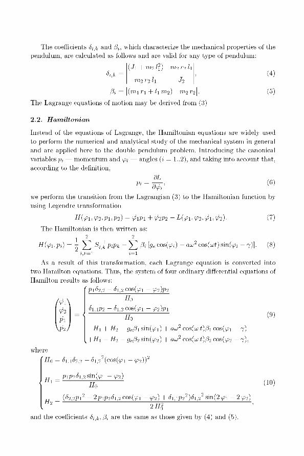
The coefficients 5^k and /%, which characterize the mechanical properties of the

pendulum, are calculated as follows and are valid for any type of pendulum:

( J i + 7712/1) 77i2 r 2 / i

m2 r2 h -h

Pi = | ( m i r i + / i m 2 ) m2r2\

The Lagrange equations of motion may be derived from (3).

2.2 . Hamiltonian

Instead of the equations of Lagrange, the Hamiltonian equations are widely used

to perform the numerical and analytical s tudy of the mechanical system in general

and are applied here to the double pendulum problem. Introducing the canonical

variables pj — momentum and ipi — angles (i = 1..2), and taking into account that ,

according to the definition,

dL Pi = dcpi''

(6)

we perform the transition from the Lagrangian (3) to the Hamiltonian function by

using Legendre transformation

H(ifl,if2,Pl,P2) = tflPl + V2P2 - L(fl, ¥>2, tfl, Wi)- (7)

The Hamiltonian is then written as: 2 2

H(fi,Pi) = - ^2 Sr^pip,, - ^ 2 (3i [gecos(<fi) - au;2 cos(u;t) sin(<fi - 7)]. (8) i,k=l i=\

As a result of this transformation, each Lagrange equation is converted into

two Hamilton equations. Thus, the system of four ordinary differential equations of

Hamilton results as follows:

>i(52,2 - tfii2 cos(y>i - f2)p2

/<P1\

¥?2

Pi

\P2/

= <

H0

8l,lP2 - #1,2 COs(yi - if2)pi

Ho

—Hi + H2 — gePi s in(yi ) + aJ2 cos{u> t)[3\ cos(y>i — 7)

^+H\ - H2 - gefh s in(^ 2 ) + aJ2 cos(cut)/32 cos(y2 - 7):

(9)

where

'H0 = £1,i(32,2 - <5i,22(cos(^i - cp2))2

PlP2^1,2Sm(ip1 - cp2) Hx

H2 =

Ho

(d2,2Pi2 ~ 2piP2di,2 cos(yi - y>2) + ^i,iP22)<^i,22 sin(2 y>i - 2 y>2) 2H2

(10)

and the coefficients (5^, /% are the same as those given by (4) and (5).

The equations of Hamilton are more suitable to be numerically integrated than the equations of Lagrange. The goal of the numerical experiments is to com­pare with the experimental ones. The mean values of angles ipi (t = 0), which were measured in experiments, can be used as initial values of angles. This cannot be said about the initial values of velocity due to the vibrations of the suspension point of the pendulum.

In some cases, we used a system of equations similar to the equations of Hamilton (9) and (10) that can be obtained for averaged motion of the pendulum, using the expression for the effective potential energy that will be given in Eq. (12).

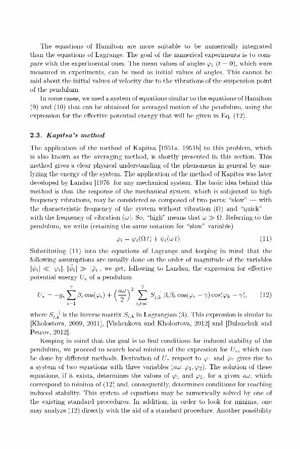
2.3. Kapitsa's method

The application of the method of Kapitsa [1951a, 1951b] to this problem, which is also known as the averaging method, is shortly presented in this section. This method gives a clear physical understanding of the phenomena in general by ana­lyzing the energy of the system. The application of the method of Kapitsa was later developed by Landau [1976] for any mechanical system. The basic idea behind this method is that the response of the mechanical system, which is subjected to high frequency vibrations, may be considered as composed of two parts: "slow" — with the characteristic frequency of the system without vibration (f2) and "quick" — with the frequency of vibration (u>). So, "high" means that u> 3> fi. Referring to the pendulum, we write (retaining the same notation for "slow" variable)

•^i = ipi(Qt) + ^i(ujt). (11)

Substituting (11) into the equations of Lagrange and keeping in mind that the following assumptions are usually done on the order of magnitude of the variables IV'il ^ IVil; IV'il ^ Iv l) w e Set) following to Landau, the expression for effective potential energy Ue of a pendulum

2 2 2

Ue = -ge^2Picos(<fi) + ( — J Y^ s7,k fjifjk cos(<fi - 7)cos(^>fc - 7), (12) i=l i,k=l

where S^k is the inverse matrix S ^ in Lagrangian (3). This expression is similar to [Kholostova, 2009, 2011], [Vishenkova and Kholostova, 2012] and [Bulanchuk and Petrov, 2012].

Keeping in mind that the goal is to find conditions for induced stability of the pendulum, we proceed to search local minima of the expression for Ue, which can be done by different methods. Derivation of Ue respect to <pi and y>2 gives rise to a system of two equations with three variables (au>,ipi,ip2). The solution of these equations, if it exists, determines the values of <pi and y>2, for a given au>, which correspond to minima of (12) and, consequently, determines conditions for reaching induced stability. This system of equations may be numerically solved by one of the existing standard procedures. In addition, in order to look for minima, one may analyze (12) directly with the aid of a standard procedure. Another possibility

consists in the numerical integration of the Hamilton equations around the points which are neighbored to the expected points of the minimum. All these methods have been examined and have given the same results. The results of this analysis will be compared below with the experiments.

The system of the differential equations (9) and (10) have been numerically solved by using MATLAB's standard procedure (ode45) and checked with Runge-Kutta method (6th order), giving the same results. The search for minima of Ue

has been carried out by using another MATLAB subroutine (Jminsearch).

2.4. Experimental set-up and procedure

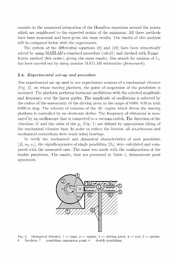
The experimental set-up used in our experiments consists of a mechanical vibrator (Fig. 2), on whose moving platform, the point of suspension of the pendulum is mounted. The platform performs harmonic oscillations with the selected amplitude and frequency over the linear guides. The amplitude of oscillations is selected by the radius of the eccentricity of the driving pivot in the range of 0.001-0.01 m with 0.001m step. The velocity of rotation of the AC engine which drives the moving platform is controlled by an electronic device. The frequency of vibrations is mea­sured by an oscilloscope that is connected to a vacuum switch. The direction of the vibration w and the value of the ge (Fig. 1) are defined by appropriate tilting of the mechanical vibrator base. In order to reduce the friction, all attachments and mechanical connections were made using bearings.

To verify the mechanical and dynamical characteristics of each pendulum (Jj,mj,rj), the eigenfrequencies of single pendulum (fij) were calculated and com­pared with the measured ones. The same was made with the configuration of the double pendulum. The results, that are presented in Table 1, demonstrate good agreement.

Fig. 2. Mechanical vibrator: 1 — base, 2 — engine, 3 — driving pivot, 4 — rod, 5 — guides, 6 — brackets, 7 — pendulum suspension point, 8 — double pendulum.

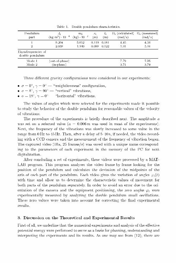
Table 1. Double pendulum characteristics.

Pendulum part

1 2

•h (kg m2) • 1CT4

9.204 2.038

mi (kg) • lO"5

5.052 1.940

(m)

0.119 0.098

k (m)

0.181 0.122

Hi (calculated) (rad/s)

4.45 5.31

Hi (measured) (rad/ s)

4.56 5.34

Eigenfrequencies of double pendulum

Mode 1 Mode 2

(out-of-phase) (in-phase)

7.79 3.71

7.35 3.79

Three different gravity configurations were considered in our experiments:

• a = 0°, 7 = 0° — "weightlessness" configuration. • a = 8°, 7 = 90° — "vertical" vibrations. • <T=18°, 7 = 0° — "horizontal" vibrations.

The values of angles which were selected for the experiments made it possible to study the behavior of the double pendulum for reasonable values of the velocity of vibrations.

The procedure of the experiments is briefly described next. The amplitude a was set on a selected value (a = 0.006m was used in most of the experiments). Next, the frequency of the vibrations was slowly increased to some value in the range from 0 Hz to 45 Hz. Then, after a delay of 5-10 s, if needed, the video record­ing with a CCD camera and the measurement of the frequency of vibration began. The captured video (10 s, 25 frames/s) was saved with a unique name correspond­ing to the parameters of each experiment in the memory of the PC for next digitalization.

After concluding a set of experiments, these videos were processed by a MAT-LAB program. This program analyses the video frame-by-frame looking for the position of the pendulum and calculates the deviation of the midpoints of the axis of each part of the pendulum. Each video gives the variation of angles <pi(t) with time and allow us to determine the characteristic values of movement for both parts of the pendulum separately. In order to avoid an error due to the ori­entation of the camera and the equipment positioning, the zero angles <pi were experimentally measured by analyzing the double pendulum small oscillations. These zero values were taken into account for correcting the final experimental results.

3. Discussion on the Theoretical and Experimental Results

First of all, we underline that the numerical experiments and analysis of the effective potential energy were performed to serve as a basis for planning, understanding and interpreting the experiments and its results. As one may see from (12), there are

two functions that depend on the angles 2

fi = ^2l3iCos(ifii), (13) i=i

2

h = J2 S^,k Pifa COS(^i - 7) COs( >fc - 7) (14) i,k=l

and both create peculiar configuration of the potential energy. It is easy to see that the function f\ determines one stable (ipi = 0°) and three unstable configurations of the pendulum ^ = [0°/180°; 180°/0°; 180°/180°]. Function f2 has four minima, which, furthermore, coincide with zeros of function at <pi = ±90° + 7. Hence, the initial knowledge on the pendulum stability may be found on the basis of prior analysis of (12)—(14).

The resulting configuration is the sum of these functions with corresponding weights: ge for f\ and (aw/2)2 for f2- The relation between weights determines the final configuration of the energy and, consequently, defines the stability of the pendulum.

3.1. Weightlessness case

The evolution of the double pendulum in weightlessness from some initial orientation to one of the equilibrium positions, which are created by vibrations, is studied in this section. This was first observed by Kapitsa [1951a, 1951b],

Analysis of the expressions (12)—(14) show that, for the weightlessness conditions and with velocity of vibrations aui = 0 the effective potential energy Ue = 0 does not depend on angles. Thus, the pendulum is at indifferent equilibrium and any value of yi and <p2 satisfy (12). We used this fact to confirm the correctness of the setting of the angle a into zero, by observing the final orientation of the pendulum after the alternative jolt impact.

Let 7 = 0 (Fig. 1) and aui ^ 0. Thus, as it is easy to see from analysis of (14), four minima of ^ ( y i , ¥2) appear. These minima are the positions of induced stability of the pendulum and, on diagram in coordinates (c^iOc^), they correspond to angles <pi = ±90° and <p2 = ±90°. Therefore, the pendulum tends to shift to one of the minimums of energy, which are now the points of induced stability. The final position, one of four minimums, and the trajectory of the pendulum, which can be drawn on diagram (c^iOc^), are defined by the initial conditions.

Photograms of Fig. 3 show two examples of the evolution of the double pendulum starting from different initial positions to the different final ones.

The videos recorded during these experiments were digitized and an example is shown in Fig. 4, where the trajectory of the pendulum (Fig. 3(a)) is presented.

As one may see, the pendulum, starting from (y>i = 136.5°, <p2 = —90.5°), moves to the final position (y>i = 90°, <p2 = 270°/—90°). Note that the second rod of the pendulum performs the complete circle around its suspension point — which is

(a) (b)

Fig. 3. Photograms of the evolution of the double pendulum in weightlessness.

not shown in the photograms. A similar behavior of the pendulum occurs with the configuration of Fig. 3(b) — where the initial and the final configurations are now different.

The results of numerical experiments, which were performed using the Hamil­ton equations for averaged movements of the pendulum, together with the real experiment are shown in Fig. 4. When looking at Fig. 4, it can be seen that the experimentally and numerically calculated trajectories show a similar behavior. The simplest model of friction has been included into the numerical code in order to con­sider the damped movement of the pendulum. Attention is drawn to the fact that the vibration forces the double pendulum to line up in the direction of vibrations [Kapitsa, 1951a, 1951b],

360

270

180

90

0

-90

180

I I

C 3 ^ ^ ^ ^ ^ ^ ^ ^ ^ ^ ^ ^ ^ ^ ^ ^ ^ ^ ^ « B - ^st^^^^^^^&ep

^k "jj

^ ^ ^ i

'£°~^L^^^^?=^=^=^^~*' ;

[ } 30 60 90 120

<Pl[

Fig. 4. Experimental (—o—) and numerical ( ) results of the evolution of pendulum in weight­lessness. Black circle — final position (Fig. 3(a)).

3.2. Vertical case

Now, the stability of the double pendulum is influenced by the gravity (ge), which changes the configuration of energy Ue of the pendulum compared with the case of weightlessness. As shown above, there exist four equilibrium positions of the pendu­lum in weightlessness and in the presence of vibrations. If the gravity is taken into account and aligned with the direction of vibrations (7 = 90°), then these four equi­libriums still exist, but three of them may be unstable and could be stabilized when the velocity of vibrations is increased enough. Figure 5 shows the energy contour plot and the equilibrium positions of the pendulum — three of them induced.

Fig. 5. Contour plot of the relative Ue in the case of vertical vibrations. The symbols correspond to the equilibrium positions. ( Q — stable, <C>, A, v — correspond to values of Table 2.)

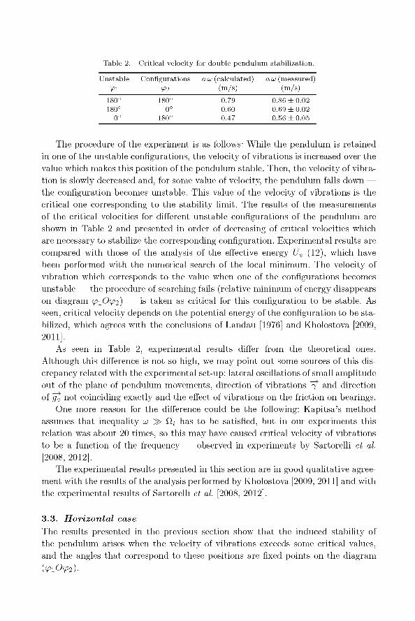
Table 2. Critical velocity for double pendulum stabilization.

Unstable Configurations a u> (calculated) a u> (measured) •-P1 ¥>2 ( m / s ) ( m / s )

f80° f80° 0.79 0.86 ±0 .02 180° 0° 0.60 0.69 ±0 .02

0° f80° 0.47 0.56 ±0 .05

The procedure of the experiment is as follows: While the pendulum is retained in one of the unstable configurations, the velocity of vibrations is increased over the value which makes this position of the pendulum stable. Then, the velocity of vibra­tion is slowly decreased and, for some value of velocity, the pendulum falls down — the configuration becomes unstable. This value of the velocity of vibrations is the critical one corresponding to the stability limit. The results of the measurements of the critical velocities for different unstable configurations of the pendulum are shown in Table 2 and presented in order of decreasing of critical velocities which are necessary to stabilize the corresponding configuration. Experimental results are compared with those of the analysis of the effective energy Ue (12), which have been performed with the numerical search of the local minimum. The velocity of vibration which corresponds to the value when one of the configurations becomes unstable — the procedure of searching fails (relative minimum of energy disappears on diagram <p\0<p2) — is taken as critical for this configuration to be stable. As seen, critical velocity depends on the potential energy of the configuration to be sta­bilized, which agrees with the conclusions of Landau [1976] and Kholostova [2009, 2011].

As seen in Table 2, experimental results differ from the theoretical ones. Although this difference is not so high, we may point out some sources of this dis­crepancy related with the experimental set-up: lateral oscillations of small amplitude out of the plane of pendulum movements, direction of vibrations 7 and direction of ge not coinciding exactly and the effect of vibrations on the friction on bearings.

One more reason for the difference could be the following: Kapitsa's method assumes that inequality u> 3> fij has to be satisfied, but in our experiments this relation was about 20 times, so this may have caused critical velocity of vibrations to be a function of the frequency — observed in experiments by Sartorelli et al. [2008, 2012].

The experimental results presented in this section are in good qualitative agree­ment with the results of the analysis performed by Kholostova [2009, 2011] and with the experimental results of Sartorelli et al. [2008, 2012],

3.3. Horizontal case

The results presented in the previous section show that the induced stability of the pendulum arises when the velocity of vibrations exceeds some critical values, and the angles that correspond to these positions are fixed points on the diagram

15

^ 5 8-

0

^w*

- \

»^X^ ®r

_JC_\ o cpl = 12.3[°] « W = - 3 . 6 [ ° ] -

J S ^ V 1 2 3 4 5 6 7

(a)

50-

oo Ci - nniD

-50-

-100-

.....^sa^fflfi

—lt&-&tf£.-

auj[m/s

(b)

1.2 1.4

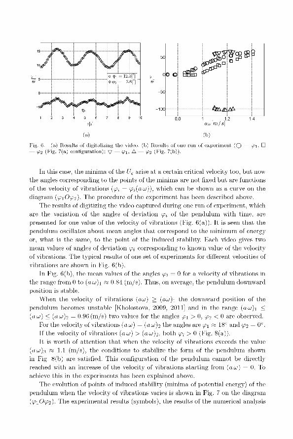
Fig. 6. (a) Results of digitalizing the video, (b) Results of one run of experiment ( O — fit C — 952 (Fig- 7(a) configuration); v — ¥>l, A — ¥2 (Fig. 7(b)).

In this case, the minima of the Ue arise at a certain critical velocity too, but now the angles corresponding to the points of the minima are not fixed but are functions of the velocity of vibrations (ipi = ipi(au>)), which can be shown as a curve on the diagram {<p\0<p2)- The procedure of the experiment has been described above.

The results of digitizing the video captured during one run of experiment, which are the variation of the angles of deviation ipi of the pendulum with time, are presented for one value of the velocity of vibrations (Fig. 6(a)). It is seen that the pendulum oscillates about mean angles that correspond to the minimum of energy or, what is the same, to the point of the induced stability. Each video gives two mean values of angles of deviation <pi corresponding to known value of the velocity of vibrations. The typical results of one set of experiments for different velocities of vibrations are shown in Fig. 6(b).

In Fig. 6(b), the mean values of the angles <pi = 0 for a velocity of vibrations in the range from 0 to (au>)i « 0.84 (m/s). Thus, on average, the pendulum downward position is stable.

When the velocity of vibrations (au>) > (aw)i the downward position of the pendulum becomes unstable [Kholostova, 2009, 2011] and in the range (auj)\ < (au>) < (auj)2 = 0.96 (m/s) two values for the angles <pi > 0, y>2 < 0 are observed.

For the velocity of vibrations (au>) = (auj)2 the angles are <pi « 18° and y>2 = 0 ° . If the velocity of vibrations (au>) > (a01)2, both ipi > 0 (Fig. 8(a)). It is worth of attention that when the velocity of vibrations exceeds the value

(au>)s « 1.1 (m/s), the conditions to stabilize the form of the pendulum shown in Fig. 8(b) are satisfied. This configuration of the pendulum cannot be directly reached with an increase of the velocity of vibrations starting from (au>) = 0. To achieve this in the experiments has been explained above.

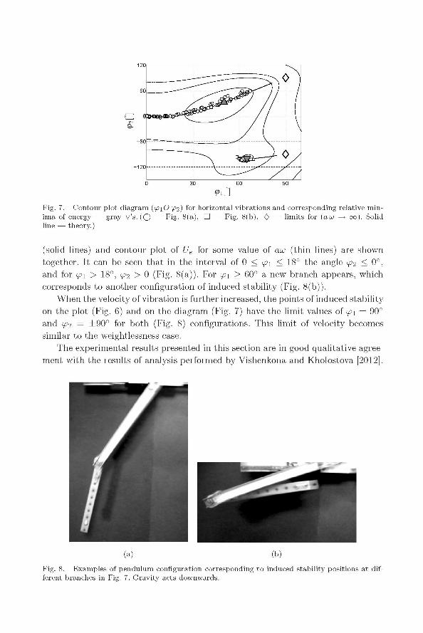
The evolution of points of induced stability (minima of potential energy) of the pendulum when the velocity of vibrations varies is shown in Fig. 7 on the diagram (ipiOip2). The experimental results (symbols), the results of the numerical analysis

0 30 60 90

<Pl[°]

Fig. 7. Contour plot diagram (ipiO (P2) f° r horizontal vibrations and corresponding relative min­ima of energy — gray V's. ( O — Fig- 8(a), • — Fig. 8(b), <0> — limits for (au> —> oo). Solid line — theory.)

(solid lines) and contour plot of Ue for some value of aui (thin lines) are shown together. It can be seen that in the interval of 0 < <pi < 18° the angle y>2 < 0°. and for <pi > 18°, y>2 > 0 (Fig. 8(a)). For <pi > 60° a new branch appears, which corresponds to another configuration of induced stability (Fig. 8(b)).

When the velocity of vibration is further increased, the points of induced stability on the plot (Fig. 6) and on the diagram (Fig. 7) have the limit values of <pi = 90° and ip2 = ±90° for both (Fig. 8) configurations. This limit of velocity becomes similar to the weightlessness case.

The experimental results presented in this section are in good qualitative agree­ment with the results of analysis performed by Vishenkona and Kholostova [2012],

(a) (b)

Fig. 8. Examples of pendulum configuration corresponding to induced stability positions at dif­ferent branches in Fig. 7. Gravity acts downwards.

4. Con c lu s ion

This paper has presented the experimental and theoretical results of dynamics and

stability of the double pendulum. Different cases were considered: weightlessness,

which was simulated by positioning the pendulum oscillating plane in parallel to

the horizontal one; vertical, when the directions of gravity and vibrations are par­

allel, and horizontal, when the direction of vibrations forms a right angle with

gravity.

(a) It was shown tha t in the weightlessness case, the profile of the potential

energy of the system varies in the presence of vibrations in such a manner tha t the

double pendulum is forced to align with the direction of vibrations. Then induced

stability configurations of the pendulum are generated.

(b) The critical velocities of vibration were measured for unstable configura­

tions of the pendulum in the case of vertical vibrations. It was shown tha t the

critical velocities depend on the configuration of the pendulum. Measured critical

velocities are compared with the numerical ones and with published theoretical and

experimental results.

(c) In the horizontal case, the relation between the angles of equilibrium and the

velocity of vibrations was studied and, as shown, the vibrations affect the induced

stability of the pendulum, creating new stable configurations of the pendulum.

In general, experimental and numerical results are in good agreement. Qualita­

tive and not quanti tat ive agreement, with other authors is due to the differences in

the mechanical properties of the pendulums (4) and (5).

R e f e r e n c e s

Acheson, D. J. and Mullin, T. [1993] "Upside-down pendulums," Natute 366, 215-216. Aguilar, J. J., Lee, G., Marcotte, C , Suri, B. [2015] "Inverted pendulum,"

http://nldlab.gatech.edu/w/index.php?title=Group_7. Bulanchuk, P. O. and Petrov, A. G. [2012] "Control of the equilibrium point of simple

and double mathematical pendulums with oblique vibration," Doklady Physics 57(2), 73-77; ISSN 1028-3358.

Kalmus, H. P. [1970] "The inverted pendulum," American Journal of Physics 38(7), 874-878.

Kapitsa, P. L. [1951a] "Dynamic stability of a pendulum with an oscillating point of suspen­sion," Journal of Experimental and Theoretical Physics 21(5), 588-597 (in Russian).

Kapitsa, P. L. [1951b] "Pendulum with an oscillating point of suspension," Uspekhi Fizich-eskih Nauk 44(1), 7-20 (in Russian).

Kholostova, O. V. [2009] "On motions of a double pendulum with a vibrating suspension point," Izvestia Rossiiskoi Akademii Nauk, Mekhanika Tverdogo Tela 2, 25-40.

Kholostova, O. V. [2011] "On stability of relative equilibria of a double pendulum with vibrating suspension point," Mechanics of Solids 46(4), 508-518.

Landau, L. D. and Lifshits, E. M. [1976] Mechanics (Pergamon Press, New York). Levein, R. B. and Tan, S. M. [1993] "Double pendulum: An experiment in chaos," American

Journal of Physics 61(11), 1038-1044. Lowenstern, E. R. [1932] "The stabilizing effect of imposed oscillations of high frequency

on a dynamic system," Philosophical Magazine and Journal of Science 8, 458-486.

Sartorelli, J. C , Serminaro, B. and Lacarbonara, W. [2008] "Parametric double pendu­lum," Sixth EUROMECH Nonlinear Dynamics Conference, Saint Petersburg, Russia, 30 June-4 July, pp. 1-4.

Sartorelli, J. C. and Lacarbonara, W. [2012] "Parametric resonances in a base-excited double pendulum," Nonlinear Dynamics 69, 1679-1692.

Smith, H. J. T. and Blackburn, J. A. [1992] "Experimental study of an inverted pendulum," American Journal of Physics 60(10), 909-911.

Stephenson, A. [1908a] "On a new type of dynamical stability," Memoirs and Proceedings of the Manchester Literary and Philosophical Society 52(8), 1-10.

Stephenson, A. [1908b] "On induced stability," Philosophical Magazine and Journal of Science 15(6), 233-236.

Stephenson, A. [1909] "On induced stability," Philosophical Magazine and Journal of Sci­ence 17, 765-766.

Vishenkova, E. A. and Kholostova, O. V. [2012] "To dynamics of a double pendulum with a horizontally vibrating point of suspension," Vestnik Udmurtskogo Universiteta 2, 114-129 (in Russian).

Vasilkov, V., Chubinsky, K. and Yakimova, K. [2007] "The Stephenson-Kapitsa pendulum: Area of the attraction of the upper positions of the balance," Technische Mechanik 27(1), 61-66.