Geophys. J. Int. (2021) 225, 926–949 doi: 10.1093/gji/ggab017 Advance Access publication 2021 January 13 GJI Seismology Double-difference seismic attenuation tomography method and its application to The Geysers geothermal field, California Hao Guo and Clifford Thurber Department of Geoscience, University of Wisconsin-Madison, 1215 W. Dayton St., Madison, WI 53706, USA. E-mail: [email protected] Accepted 2021 January 11. Received 2020 December 16; in original form 2020 August 1 SUMMARY Knowledge of attenuation structure is important for understanding subsurface material prop- erties. We have developed a double-difference seismic attenuation (DDQ) tomography method for high-resolution imaging of 3-D attenuation structure. Our method includes two main ele- ments, the inversion of event-pair differential t ∗ (dt ∗ ) data and 3-D attenuation tomography with the dt ∗ data. We developed a new spectral ratio method that jointly inverts spectral ratio data from pairs of events observed at a common set of stations to determine the dt ∗ data. The spectral ratio method cancels out instrument and site response terms, resulting in more accurate dt ∗ data compared to absolute t ∗ from traditional methods using individual spectra. Synthetic tests show that the inversion of dt ∗ data using our spectral ratio method is robust to the choice of source model and a moderate degree of noise. We modified an existing velocity tomography code so that it can invert dt ∗ data for 3-D attenuation structure. We applied the new method to The Geyser geothermal field, California, which has vapour-dominated reservoirs and a long history of water injection. A new Qp model at The Geysers is determined using P-wave data of earthquakes in 2011, using our updated earthquake locations and Vp model. By taking advantage of more accurate dt ∗ data and the cancellation of model uncertainties along the common paths outside of the source region, the DDQ tomography method achieves higher resolution, especially in the earthquake source regions, compared to the standard tomography method using t ∗ data. This is validated by both the real and synthetic data tests. Our Qp and Vp models show consistent variations in a normal temperature reservoir that can be explained by variations in fracturing, permeability and fluid saturation and/or steam pressure. A promi- nent low-Qp and Vp zone associated with very active seismicity is imaged within a high temperature reservoir at depths below 2 km. This anomalous zone is likely partially saturated with injected fluids. Key words: Body waves; Seismic attenuation; Seismic tomography. 1 INTRODUCTION Compared to seismic compressional and shear wave velocities (Vp and Vs), seismic attenuation, represented by seismic quality fac- tor Q, is more sensitive to rock properties related to pores, cracks, fractures and fluids. A popular way to determine subsurface 3-D Q structure is to invert observed earthquake spectra for path attenu- ation terms, t ∗ , from a set of earthquakes at a set of stations and then perform 3-D Q tomography with the obtained t ∗ data. The recorded seismogram is affected by two types of attenuation, in- trinsic attenuation and scattering attenuation (Sato & Fehler 2009). Intrinsic attenuation is the energy loss of seismic waves when pass- ing through rocks. Intrinsic attenuation is highly influenced by rock porosity, pore shape, pore density, permeability, saturation, con- fining pressure and pore pressure (O’Connell & Budiansky 1977; Winkler & Nur 1979; Peacock et al. 1994). Intrinsic attenuation is weekly dependent on frequency within the seismic frequency band according to lab experiments (e.g. Fail & Jackson 2015) and seismic observations (e.g. Pozgay et al. 2009; Wei & Wiens 2018). Scatter- ing attenuation is the energy redistribution of seismic waves when being converted, reflected, or refracted by small-scale scatterers. Scattering attenuation can be frequency dependent, depending on the size of scatterers relative to the wavelength (Frankel 1991). Most standard Q tomography methods use absolute t ∗ data that are inverted from single spectrum data for individual earth- quakes observed at individual stations (Scherbaum 1990; Rietbrock 1996; Thurber & Eberhart-Phillips 1999; Rietbrock 2001; Eberhart- Phillips & Chadwick 2002; Pozgay et al. 2009; Liu et al. 2014) or for groups of earthquakes observed at groups of stations (Benning- ton et al. 2008; Bisrat et al. 2014; Ohlendorf et al. 2014). Since the inversion of t ∗ data is coupled to instrument response, site response and source parameters, some methods using spectral ratio data have been used to remove some coupling effects to determine more accu- rate differential t ∗ (dt ∗ ) data, which also can be used to estimate Q 926 C The Author(s) 2021. Published by Oxford University Press on behalf of The Royal Astronomical Society. All rights reserved. For permissions, please e-mail: [email protected] Downloaded from https://academic.oup.com/gji/article/225/2/926/6095732 by guest on 15 July 2022

Welcome message from author
This document is posted to help you gain knowledge. Please leave a comment to let me know what you think about it! Share it to your friends and learn new things together.
Transcript
Geophys. J. Int. (2021) 225, 926–949 doi: 10.1093/gji/ggab017Advance Access publication 2021 January 13GJI Seismology
Double-difference seismic attenuation tomography method and itsapplication to The Geysers geothermal field, California
Hao Guo and Clifford ThurberDepartment of Geoscience, University of Wisconsin-Madison, 1215 W. Dayton St., Madison, WI 53706, USA. E-mail: [email protected]
Accepted 2021 January 11. Received 2020 December 16; in original form 2020 August 1
S U M M A R YKnowledge of attenuation structure is important for understanding subsurface material prop-erties. We have developed a double-difference seismic attenuation (DDQ) tomography methodfor high-resolution imaging of 3-D attenuation structure. Our method includes two main ele-ments, the inversion of event-pair differential t∗ (dt∗) data and 3-D attenuation tomographywith the dt∗ data. We developed a new spectral ratio method that jointly inverts spectral ratiodata from pairs of events observed at a common set of stations to determine the dt∗ data.The spectral ratio method cancels out instrument and site response terms, resulting in moreaccurate dt∗ data compared to absolute t∗ from traditional methods using individual spectra.Synthetic tests show that the inversion of dt∗ data using our spectral ratio method is robust tothe choice of source model and a moderate degree of noise. We modified an existing velocitytomography code so that it can invert dt∗ data for 3-D attenuation structure. We applied the newmethod to The Geyser geothermal field, California, which has vapour-dominated reservoirsand a long history of water injection. A new Qp model at The Geysers is determined usingP-wave data of earthquakes in 2011, using our updated earthquake locations and Vp model. Bytaking advantage of more accurate dt∗ data and the cancellation of model uncertainties alongthe common paths outside of the source region, the DDQ tomography method achieves higherresolution, especially in the earthquake source regions, compared to the standard tomographymethod using t∗ data. This is validated by both the real and synthetic data tests. Our Qp andVp models show consistent variations in a normal temperature reservoir that can be explainedby variations in fracturing, permeability and fluid saturation and/or steam pressure. A promi-nent low-Qp and Vp zone associated with very active seismicity is imaged within a hightemperature reservoir at depths below 2 km. This anomalous zone is likely partially saturatedwith injected fluids.
Key words: Body waves; Seismic attenuation; Seismic tomography.
1 I N T RO D U C T I O N
Compared to seismic compressional and shear wave velocities (Vpand Vs), seismic attenuation, represented by seismic quality fac-tor Q, is more sensitive to rock properties related to pores, cracks,fractures and fluids. A popular way to determine subsurface 3-D Qstructure is to invert observed earthquake spectra for path attenu-ation terms, t∗, from a set of earthquakes at a set of stations andthen perform 3-D Q tomography with the obtained t∗ data. Therecorded seismogram is affected by two types of attenuation, in-trinsic attenuation and scattering attenuation (Sato & Fehler 2009).Intrinsic attenuation is the energy loss of seismic waves when pass-ing through rocks. Intrinsic attenuation is highly influenced by rockporosity, pore shape, pore density, permeability, saturation, con-fining pressure and pore pressure (O’Connell & Budiansky 1977;Winkler & Nur 1979; Peacock et al. 1994). Intrinsic attenuation isweekly dependent on frequency within the seismic frequency band
according to lab experiments (e.g. Fail & Jackson 2015) and seismicobservations (e.g. Pozgay et al. 2009; Wei & Wiens 2018). Scatter-ing attenuation is the energy redistribution of seismic waves whenbeing converted, reflected, or refracted by small-scale scatterers.Scattering attenuation can be frequency dependent, depending onthe size of scatterers relative to the wavelength (Frankel 1991).
Most standard Q tomography methods use absolute t∗ datathat are inverted from single spectrum data for individual earth-quakes observed at individual stations (Scherbaum 1990; Rietbrock1996; Thurber & Eberhart-Phillips 1999; Rietbrock 2001; Eberhart-Phillips & Chadwick 2002; Pozgay et al. 2009; Liu et al. 2014) orfor groups of earthquakes observed at groups of stations (Benning-ton et al. 2008; Bisrat et al. 2014; Ohlendorf et al. 2014). Since theinversion of t∗ data is coupled to instrument response, site responseand source parameters, some methods using spectral ratio data havebeen used to remove some coupling effects to determine more accu-rate differential t∗ (dt∗) data, which also can be used to estimate Q
926C© The Author(s) 2021. Published by Oxford University Press on behalf of The Royal Astronomical Society. All rights reserved. Forpermissions, please e-mail: [email protected]
Dow
nloaded from https://academ
ic.oup.com/gji/article/225/2/926/6095732 by guest on 15 July 2022
Double-difference seismic attenuation tomography 927
structure. There are four kinds of spectral ratio methods, includingstation-pair, event-pair, phase-pair and event pair-station pair (ordouble-pair) spectral ratios. The station-pair method takes the ratioof spectra from individual earthquakes at pairs of stations, whichcan remove the source spectrum. The phase-pair method takes theratio of two different types of waves (e.g. P and S) from individualearthquakes at individual stations. Roth et al. (1999) have a cleardiscussion of the station-pair and phase-pair spectral ratio meth-ods. The event-pair method takes the ratio of spectra from pairs ofevents at individual stations, which can remove the instrument re-sponse and site response. Many studies (e.g. Imanishi & Ellsworth2006; Abercrombie 2014; Liu et al. 2014) used event-pair spectralratio data to estimate corner frequency and stress drop for co-locatedearthquakes from direct or coda waves but did not solve for path at-tenuation, which could be removed due to the overlapping ray paths.Shiina et al. (2018) and Kriegerowski et al. (2019) used event-pairspectral ratio data to directly solve for average path attenuation inthe earthquake source region. The double-pair method uses spectralratio data from pairs of earthquakes at pairs of stations to invertfor dt∗ and then fit dt∗ data for all pairs of events in a cluster toestimate the average attenuation in the fault zone (Blakeslee et al.1989). The method of Blakeslee et al. (1989) has a strict requirementon the distribution of events and stations relative to the fault zone.Zhang et al. (2007) used double-pair spectral ratio data to obtain dt∗
data, analogous to the method of Blakeslee et al. (1989), but thenperformed a tomographic inversion to determine 3-D Q structure.
In this paper, we develop a double-difference (DD) attenua-tion (DDQ) tomography method. Our DDQ tomography methodincludes two main parts: (1) extracting dt∗ data using a new event-pair spectral ratio method, and (2) performing 3-D Q tomographywith the obtained dt∗ data. Our spectral ratio method jointly in-verts for all source and attenuation parameters using spectral ratiosfrom pairs of events observed at common stations. Instead of usingdt∗ data to determine the average attenuation in the source region,which requires special distributions of ray paths (Shiina et al. 2018;Kriegerowski et al. 2019), we use them for a tomographic inversionfor 3-D Q structure without such a requirement. Compared to thestandard Q tomography method using absolute t∗ data, our DDQtomography method can determine higher resolution Q structurefor two reasons: (1) higher quality of dt∗ data from spectral ratioinversions; and (2) event-pair dt∗data can cancel out the effect ofmodel uncertainties along the common ray path outside the sourceregion, so that the source-region structure can be better imaged.
We first tested our spectral ratio method with noise-free andnoise-added synthetic data. Then, we applied our DDQ tomographymethod to The Geysers geothermal field, the largest geothermalfield in the world, and tested its performance with synthetic andreal data. We also updated the earthquake locations and 3-D Vpmodel. We selected The Geysers for a number of reasons. (1) TheGeysers has vapour-dominated reservoirs and has a long historyof water injection to enhance the steam production associated withvery active induced seismicity (Hartline et al. 2016). Due to highsensitivity of attenuation to saturation conditions of rocks, The Gey-sers is an ideal area to test whether our DDQ tomography methodcan image subsurface steam reservoirs and water injection zones.(2) The cancellation of site response using our spectral ratio methodis particularly important for The Geysers due to the very strong siteresponse there (Romero et al. 1997). (3) The seismic network atThe Geysers is relatively dense. A 34-station seismic network hasbeen operated by Lawrence Berkeley National Laboratory (Majer &Peterson 2007) and the waveform data are available from the North-ern California Earthquake Data Center. (4) Many velocity and Q
tomography studies have been done at The Geysers (O’Connell &Johnson 1991; Zucca et al. 1994; Romero et al. 1995; Julian et al.1996; Romero et al. 1997; Gritto et al. 2013; Jeanne et al. 2015;Lin & Wu 2018; Hutchings et al. 2019; Gritto et al. 2020). We cancompare our new Q model with previous models to see if their over-all structures are similar and if our new model has higher resolutionin earthquake source regions.
In this study, we assume frequency independent Q. Since previ-ous Q tomography studies at The Geysers also assumed frequencyindependent Q (Zucca et al. 1994; Romero et al. 1997; Hutchingset al. 2019), we can directly compare our Q model with previousQ models. However, frequency dependent Q may be the case forThe Geysers, which is dominated by steam and fluid filled poresand fractures. Eberhart-Phillips et al. (2014) show that, to firstorder, if Q is frequency dependent, that is,Q = Q0 f α , whereα ranges from 0 to 1, then the Q model obtained by inverting t∗
values assuming frequency independence approximately differs bya multiplicative scale factor from the correct frequency dependentQ model (Q0). This means that the pattern of Q variations is correctbut the absolute values of Q are not. This should also be the casefor inverting dt∗ data. Furthermore, in a previous Q tomographystudy at The Geysers, Romero et al. (1997) argued that assumingfrequency independent Q was appropriate.
2 M E T H O D O L O G Y
In this section, we first describe the methodology of extractingabsolute t∗ data using the single spectrum method and dt∗ datausing the spectral ratio method. We then describe the methodologyof DDQ tomography with absolute t∗ and dt∗ data.
2.1 Fitting event-pair spectral ratio for dt∗
The observed amplitude spectrum Aik( f ) of an earthquake i at
station k for frequency f can be expressed as (Scherbaum 1990)
Aik ( f ) = Si ( f ) Ik ( f ) Rk ( f ) Bi
k ( f ) (1)
where Si ( f ) is the source spectrum, Ik( f ) is the instrument re-sponse, Rk( f ) is the local site amplification (site response) andBi
k( f )is the attenuation spectrum that describes the wave amplitudeloss along the ray path. The source spectrum for earthquake i canbe expressed as
Si ( f ) = �ik0
1 + (f/ f i
c
)γ (2)
where �ik0 is the zero-frequency spectral level for earthquake i at
station k, accounting for the effects of radiation pattern and geomet-ric spreading, f i
c is the source corner frequency and γ represents thehigh-frequency decay factor, which is 2 for a Brune ω2 type sourcemodel (Brune 1970). Assuming frequency independent attenuation,the attenuation spectrum can be expressed as
Bik ( f ) = e−π f t∗ik (3)
where t∗ik is the whole path attenuation operator.
With eqs (2) and (3), the velocity amplitude spectrum (eq. 1) canbe expressed as
Aik ( f ) = Ik ( f ) Rk ( f )
�ik0
1 + (f/ f i
c
)γ e−π f t∗ik (4)
where Rk( f ), �ik0 , f i
c and t∗ik are the unknowns, and Ik( f ) is known
in principle. This is the basic equation for all the methods that
Dow
nloaded from https://academ
ic.oup.com/gji/article/225/2/926/6095732 by guest on 15 July 2022
928 H. Guo and C. Thurber
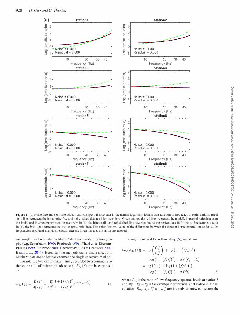
Figure 1. (a) Noise-free and (b) noise-added synthetic spectral ratio data in the natural logarithm domain as a function of frequency at eight stations. Blacksolid lines represent the input noise-free and noise-added data used for inversions. Green and red dashed lines represent the modelled spectral ratio data usingthe initial and inverted parameters, respectively. In (a), the black solid and red dashed lines overlap due to the perfect data fit for noise-free synthetic tests.In (b), the blue lines represent the true spectral ratio data. The noise (the rms value of the differences between the input and true spectral ratios for all thefrequencies used) and final data residual after the inversion at each station are labelled.
use single spectrum data to obtain t∗ data for standard Q tomogra-phy (e.g. Scherbaum 1990; Rietbrock 1996; Thurber & Eberhart-Phillips 1999; Rietbrock 2001; Eberhart-Phillips & Chadwick 2002;Bisrat et al. 2014). Hereafter, the methods using single spectra toobtain t∗ data are collectively termed the single spectrum method.
Considering two earthquakes i and j recorded by a common sta-tion k, the ratio of their amplitude spectra, RAk ( f ), can be expressedas
RAk ( f ) = Aik ( f )
A jk ( f )
= �ik0
�jk0
1 + (f/ f j
c
)γ
1 + (f/ f i
c
)γ e−π f
(t∗ik−t∗jk
)(5)
Taking the natural logarithm of eq. (5), we obtain
log(RAk ( f )
) = log
(�ik
0
�jk0
)+ log
(1 + (
f/ f jc
)γ )−log
(1 + (
f/ f ic
)γ ) − π f(t∗ik − t∗
jk
)= log
(R�k
) + log(1 + (
f/ f jc
)γ )−log
(1 + (
f/ f ic
)γ ) − π f dt∗k (6)
where R�k is the ratio of low-frequency spectral levels at station kand dt∗
k = t∗ik − t∗
jk is the event-pair differential t∗ at station k. In thisequation, R�k , f i
c , f jc and dt∗
k are the only unknowns because the
Dow
nloaded from https://academ
ic.oup.com/gji/article/225/2/926/6095732 by guest on 15 July 2022

Double-difference seismic attenuation tomography 929
Figure 1. (Continued.)
instrument response and site response terms cancel out. Since therelationship between the spectral ratio and the source parametersis nonlinear, the Levenberg–Marquardt (LM) method (Aster et al.2019), an iterative, damped least squares method, can be used tosolve the spectral ratio equation for the unknowns. First, we usea truncated Taylor series approximation to linearize the differencebetween observed and calculated values, rk , for eq. (6), as follows
rk = log(Robs
Ak
) − log(Rcal
Ak
)= ∂
[log
(RAk
)]∂ f i
c
� f ic + ∂
[log
(RAk
)]∂ f j
c
� f jc
+ ∂[log
(RAk
)]∂ R�k
�R�k + ∂[log
(RAk
)]∂dt∗
k
�dt∗k (7)
for a given estimate of the parameter values. The partial derivativesof the spectral ratio with respect to the unknowns in eq. (7) can be
expressed as
∂[log
(RAk
)]∂ f i
c
= γ
(1
f γ+ 1(
f ic
)γ
)−1(f ic
)−γ−1(7a)
∂[log
(RAk
)]∂ f j
c
= −γ
⎛⎝ 1
f γ+ 1(
f jc
)γ
⎞⎠
−1(f jc
)−γ−1(7b)
∂[log
(RAk
)]∂ R�k
= 1
R�k
(7c)
∂[log
(RAk
)]∂dt∗
k
= −π f (7d)
Dow
nloaded from https://academ
ic.oup.com/gji/article/225/2/926/6095732 by guest on 15 July 2022

930 H. Guo and C. Thurber
Figure 2. The evolution of inverted dt∗ with iterations for (a)–(c) noise-free and (d)–(f) noise-added synthetic tests that generated synthetic spectral ratio datawith γ values of (a) and (d) 2, (b) and (e) 1.5, and (c) and (f) 2.5 and used a γ value of 2 for inversions. Each black dashed line represents the true dt∗ at eachstation. Red dots connected by red dashed lines represent the inverted dt∗ after each iteration except for the dots at iteration 0 that represent the initial dt∗.
We solve the linear system of eq. (7) for one event pair recordedby n stations as follows,
�m = (J(m)T J (m) + λI
)−1J(m)T r (m) (8)
where �m is the vector of perturbations of the 2n + 2 unknowns(m) including n R�, n dt∗ and two fc, J(m) is the matrix of partialderivatives of spectral ratios for all usable frequencies with respectto all unknowns (the Jacobian matrix) and r(m) is the vector ofthe residuals between the observed and calculated spectral ratiosfor all usable frequencies. The Jacobian matrix and residual vec-tor are weighted based on the quality (signal-to-noise ratio, SNR)of each datum. The weighted Jacobian matrix is further processedwith column scaling to avoid the large contrast of sensitivities ofsome parameters. A damping parameter λ is used to stabilize theinversion system to facilitate the convergence of the solution. Wesearch for a λ value that can yield a moderate condition numberfor the inversion system, which is calculated by dividing the maxi-mum singular value by the minimum singular value and used as anindicator of the stability of the least-squares inversion (Aster et al.2019).
The initial parameters m0 can be obtained from the inversionusing a single spectrum method to solve for �0, t∗ and fc (e.g.
Bisrat et al. 2014). At each iteration i , we update the model,mi = mi−1 + �m, recalculate the residual vector and Jacobianmatrix, and determine the new perturbation �m. The inversionstops when the norm of the residual vector no longer decreasessignificantly.
2.2 DDQ tomography
Assuming frequency independent attenuation, the whole path atten-uation operator t∗ from event i to station k can expressed as a pathintegral as follows (Scherbaum 1990),
t∗ik = tik
Qik=
∫ k
iuQ−1dl + sk (9)
where tik is the traveltime, Qik is the whole path dimensionlessquality factor Q along the ray path, u represents the slowness (thereciprocal of velocity), dl is an element of path length and sk isa station correction term accounting for unmodelled structure nearthe surface below station k. Solving for the attenuation structure is astandard seismic tomography problem analogous to solving for seis-mic velocity structure with source locations fixed. Although eq. (9)can be solved directly for Q−1, we determine the perturbations of
Dow
nloaded from https://academ
ic.oup.com/gji/article/225/2/926/6095732 by guest on 15 July 2022
Double-difference seismic attenuation tomography 931
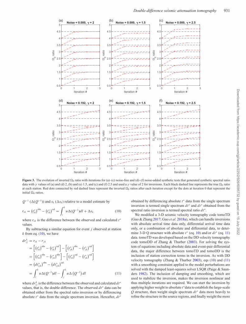
Figure 3. The evolution of inverted �0 ratio with iterations for (a)–(c) noise-free and (d)–(f) noise-added synthetic tests that generated synthetic spectral ratiodata with γ values of (a) and (d) 2, (b) and (e) 1.5, and (c) and (f) 2.5 and used a γ value of 2 for inversions. Each black dashed line represents the true �0 ratioat each station. Red dots connected by red dashed lines represent the inverted �0 ratios after each iteration except for the dots at iteration 0 that represent theinitial �0 ratios.
Q−1 (�(Q−1)) and sk (�sk) relative to a model estimate by
rik = (t∗ik
)obs − (t∗ik
)cal =∫ k
iu�(Q−1)dl + �sk (10)
where rik is the difference between the observed and calculated t∗
values.By subtracting a similar equation for event j observed at station
k from eq. (10), we have
drki j = rik − r jk
=[(
t∗ik
)obs − (t∗ik
)cal]
−[(
t∗jk
)obs − (t∗
jk
)cal]
=[(
t∗ik
)obs − (t∗
jk
)obs]
−[(
t∗ik
)cal − (t∗
jk
)cal]
= (dt∗
i jk
)obs − (dt∗
i jk
)cal
=∫ k
iu�(Q−1)dl −
∫ k
ju�
(Q−1
)dl (11)
where drki j is the difference between the observed and calculated dt∗
values, that is, the double difference. The observed dt∗ data can beobtained either from the spectral ratio inversion or by differencingabsolute t∗ data from the single spectrum inversion. Hereafter, dt∗
obtained by differencing absolute t∗ data from the single spectruminversion is termed single spectrum dt∗ and dt∗ obtained from thespectral ratio inversion is termed spectral ratio dt∗.
We modified a 3-D seismic velocity tomography code tomoTD(Guo & Zhang 2017; Guo et al. 2018a), which can handle inversionswith absolute arrival time data only, differential arrival time dataonly, or a combination of absolute and differential data, to deter-mine 3-D Q structure with absolute t∗ (eq. 10) and/or dt∗ (eq. 11)data. tomoTD was developed based on the DD velocity tomographycode tomoDD of Zhang & Thurber (2003). For solving the sys-tem of equations including absolute data and event-pair differentialdata, the major difference between tomoTD and tomoDD is theinclusion of station correction terms in the inversion. As with DDvelocity tomography (Zhang & Thurber 2003), eqs (10) and (11)with a smoothing constraint applied to the model perturbations aresolved with the damped least-squares solver LSQR (Paige & Saun-ders 1982). The inclusion of damping and smoothing, which areused to stabilize the inversion, makes the inversion nonlinear andthus multiple iterations are required. We can start the inversion byapplying higher weight to absolute t∗data to establish the large-scaleQ structure, then weight single spectrum dt∗ data more heavily torefine the structure in the source regions, and finally weight the more
Dow
nloaded from https://academ
ic.oup.com/gji/article/225/2/926/6095732 by guest on 15 July 2022
932 H. Guo and C. Thurber
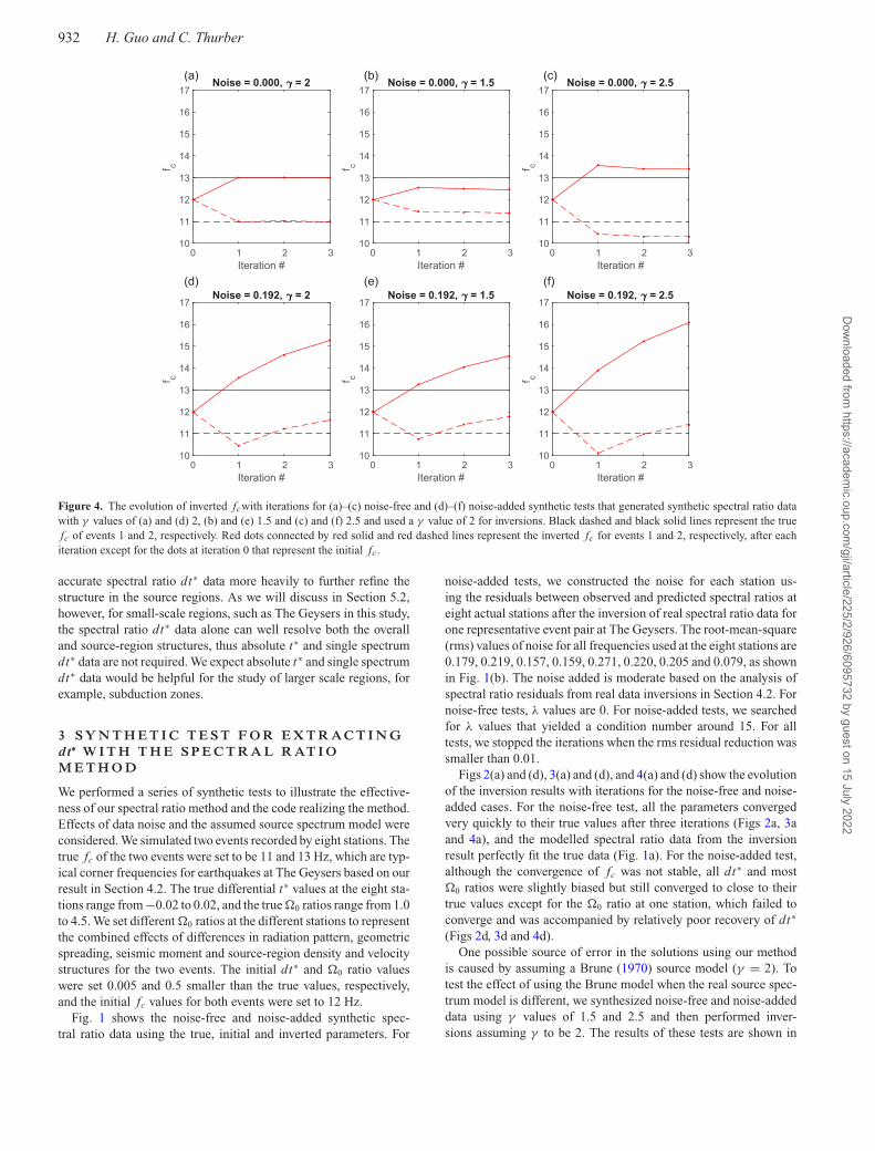
Figure 4. The evolution of inverted fcwith iterations for (a)–(c) noise-free and (d)–(f) noise-added synthetic tests that generated synthetic spectral ratio datawith γ values of (a) and (d) 2, (b) and (e) 1.5 and (c) and (f) 2.5 and used a γ value of 2 for inversions. Black dashed and black solid lines represent the truefc of events 1 and 2, respectively. Red dots connected by red solid and red dashed lines represent the inverted fc for events 1 and 2, respectively, after eachiteration except for the dots at iteration 0 that represent the initial fc .
accurate spectral ratio dt∗ data more heavily to further refine thestructure in the source regions. As we will discuss in Section 5.2,however, for small-scale regions, such as The Geysers in this study,the spectral ratio dt∗ data alone can well resolve both the overalland source-region structures, thus absolute t∗ and single spectrumdt∗ data are not required. We expect absolute t∗ and single spectrumdt∗ data would be helpful for the study of larger scale regions, forexample, subduction zones.
3 S Y N T H E T I C T E S T F O R E X T R A C T I N Gdt∗ W I T H T H E S P E C T R A L R AT I OM E T H O D
We performed a series of synthetic tests to illustrate the effective-ness of our spectral ratio method and the code realizing the method.Effects of data noise and the assumed source spectrum model wereconsidered. We simulated two events recorded by eight stations. Thetrue fc of the two events were set to be 11 and 13 Hz, which are typ-ical corner frequencies for earthquakes at The Geysers based on ourresult in Section 4.2. The true differential t∗ values at the eight sta-tions range from −0.02 to 0.02, and the true �0 ratios range from 1.0to 4.5. We set different �0 ratios at the different stations to representthe combined effects of differences in radiation pattern, geometricspreading, seismic moment and source-region density and velocitystructures for the two events. The initial dt∗ and �0 ratio valueswere set 0.005 and 0.5 smaller than the true values, respectively,and the initial fc values for both events were set to 12 Hz.
Fig. 1 shows the noise-free and noise-added synthetic spec-tral ratio data using the true, initial and inverted parameters. For
noise-added tests, we constructed the noise for each station us-ing the residuals between observed and predicted spectral ratios ateight actual stations after the inversion of real spectral ratio data forone representative event pair at The Geysers. The root-mean-square(rms) values of noise for all frequencies used at the eight stations are0.179, 0.219, 0.157, 0.159, 0.271, 0.220, 0.205 and 0.079, as shownin Fig. 1(b). The noise added is moderate based on the analysis ofspectral ratio residuals from real data inversions in Section 4.2. Fornoise-free tests, λ values are 0. For noise-added tests, we searchedfor λ values that yielded a condition number around 15. For alltests, we stopped the iterations when the rms residual reduction wassmaller than 0.01.
Figs 2(a) and (d), 3(a) and (d), and 4(a) and (d) show the evolutionof the inversion results with iterations for the noise-free and noise-added cases. For the noise-free test, all the parameters convergedvery quickly to their true values after three iterations (Figs 2a, 3aand 4a), and the modelled spectral ratio data from the inversionresult perfectly fit the true data (Fig. 1a). For the noise-added test,although the convergence of fc was not stable, all dt∗ and most�0 ratios were slightly biased but still converged to close to theirtrue values except for the �0 ratio at one station, which failed toconverge and was accompanied by relatively poor recovery of dt∗
(Figs 2d, 3d and 4d).One possible source of error in the solutions using our method
is caused by assuming a Brune (1970) source model (γ = 2). Totest the effect of using the Brune model when the real source spec-trum model is different, we synthesized noise-free and noise-addeddata using γ values of 1.5 and 2.5 and then performed inver-sions assuming γ to be 2. The results of these tests are shown in
Dow
nloaded from https://academ
ic.oup.com/gji/article/225/2/926/6095732 by guest on 15 July 2022
Double-difference seismic attenuation tomography 933
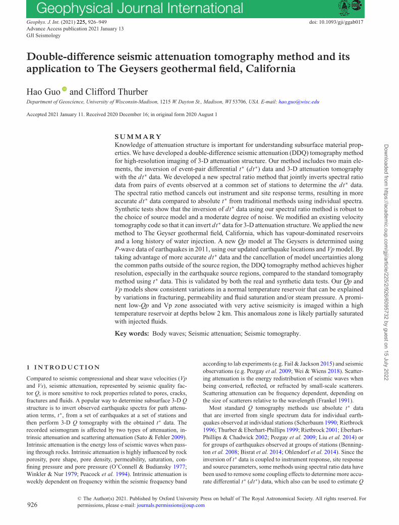
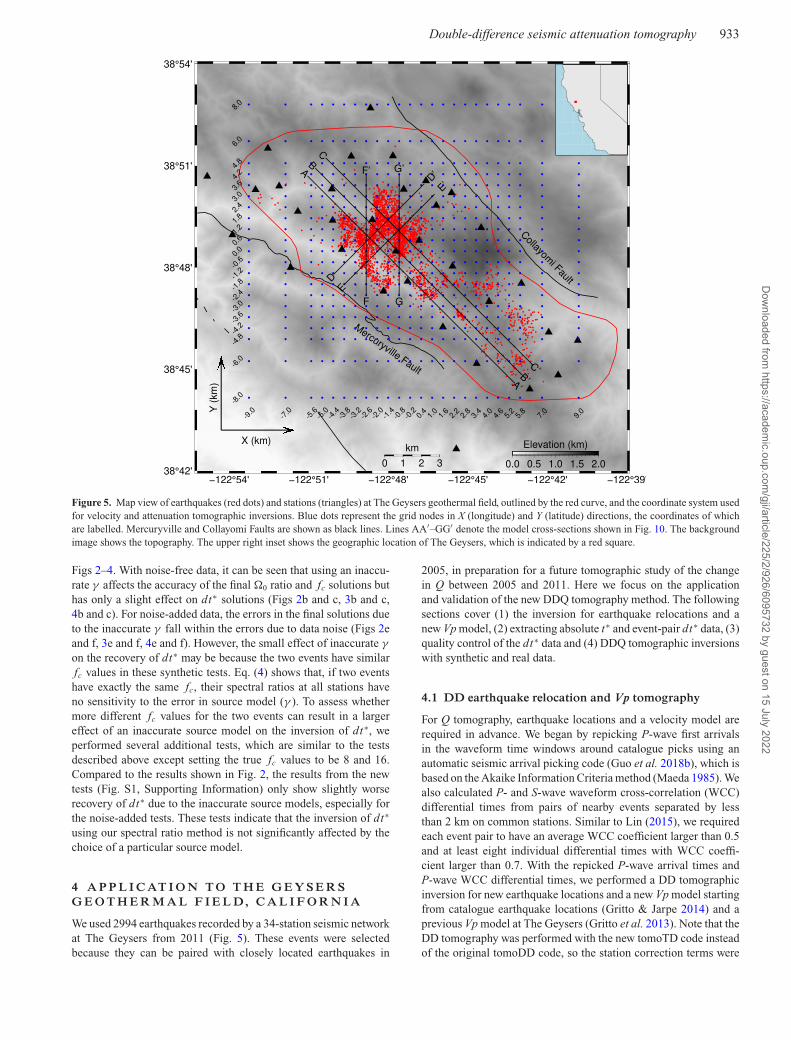
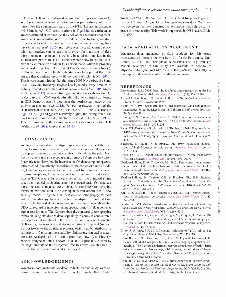
Figure 5. Map view of earthquakes (red dots) and stations (triangles) at The Geysers geothermal field, outlined by the red curve, and the coordinate system usedfor velocity and attenuation tomographic inversions. Blue dots represent the grid nodes in X (longitude) and Y (latitude) directions, the coordinates of whichare labelled. Mercuryville and Collayomi Faults are shown as black lines. Lines AA′–GG′ denote the model cross-sections shown in Fig. 10. The backgroundimage shows the topography. The upper right inset shows the geographic location of The Geysers, which is indicated by a red square.
Figs 2–4. With noise-free data, it can be seen that using an inaccu-rate γ affects the accuracy of the final �0 ratio and fc solutions buthas only a slight effect on dt∗ solutions (Figs 2b and c, 3b and c,4b and c). For noise-added data, the errors in the final solutions dueto the inaccurate γ fall within the errors due to data noise (Figs 2eand f, 3e and f, 4e and f). However, the small effect of inaccurate γ
on the recovery of dt∗ may be because the two events have similarfc values in these synthetic tests. Eq. (4) shows that, if two eventshave exactly the same fc, their spectral ratios at all stations haveno sensitivity to the error in source model (γ ). To assess whethermore different fc values for the two events can result in a largereffect of an inaccurate source model on the inversion of dt∗, weperformed several additional tests, which are similar to the testsdescribed above except setting the true fc values to be 8 and 16.Compared to the results shown in Fig. 2, the results from the newtests (Fig. S1, Supporting Information) only show slightly worserecovery of dt∗ due to the inaccurate source models, especially forthe noise-added tests. These tests indicate that the inversion of dt∗
using our spectral ratio method is not significantly affected by thechoice of a particular source model.
4 A P P L I C AT I O N T O T H E G E Y S E R SG E O T H E R M A L F I E L D, C A L I F O R N I A
We used 2994 earthquakes recorded by a 34-station seismic networkat The Geysers from 2011 (Fig. 5). These events were selectedbecause they can be paired with closely located earthquakes in
2005, in preparation for a future tomographic study of the changein Q between 2005 and 2011. Here we focus on the applicationand validation of the new DDQ tomography method. The followingsections cover (1) the inversion for earthquake relocations and anew Vp model, (2) extracting absolute t∗ and event-pair dt∗ data, (3)quality control of the dt∗ data and (4) DDQ tomographic inversionswith synthetic and real data.
4.1 DD earthquake relocation and Vp tomography
For Q tomography, earthquake locations and a velocity model arerequired in advance. We began by repicking P-wave first arrivalsin the waveform time windows around catalogue picks using anautomatic seismic arrival picking code (Guo et al. 2018b), which isbased on the Akaike Information Criteria method (Maeda 1985). Wealso calculated P- and S-wave waveform cross-correlation (WCC)differential times from pairs of nearby events separated by lessthan 2 km on common stations. Similar to Lin (2015), we requiredeach event pair to have an average WCC coefficient larger than 0.5and at least eight individual differential times with WCC coeffi-cient larger than 0.7. With the repicked P-wave arrival times andP-wave WCC differential times, we performed a DD tomographicinversion for new earthquake locations and a new Vp model startingfrom catalogue earthquake locations (Gritto & Jarpe 2014) and aprevious Vp model at The Geysers (Gritto et al. 2013). Note that theDD tomography was performed with the new tomoTD code insteadof the original tomoDD code, so the station correction terms were
Dow
nloaded from https://academ
ic.oup.com/gji/article/225/2/926/6095732 by guest on 15 July 2022
934 H. Guo and C. Thurber
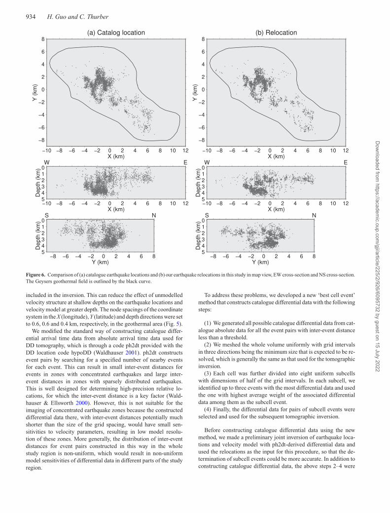
Figure 6. Comparison of (a) catalogue earthquake locations and (b) our earthquake relocations in this study in map view, EW cross-section and NS cross-section.The Geysers geothermal field is outlined by the black curve.
included in the inversion. This can reduce the effect of unmodelledvelocity structure at shallow depths on the earthquake locations andvelocity model at greater depth. The node spacings of the coordinatesystem in the X (longitude), Y (latitude) and depth directions were setto 0.6, 0.6 and 0.4 km, respectively, in the geothermal area (Fig. 5).
We modified the standard way of constructing catalogue differ-ential arrival time data from absolute arrival time data used forDD tomography, which is through a code ph2dt provided with theDD location code hypoDD (Waldhauser 2001). ph2dt constructsevent pairs by searching for a specified number of nearby eventsfor each event. This can result in small inter-event distances forevents in zones with concentrated earthquakes and large inter-event distances in zones with sparsely distributed earthquakes.This is well designed for determining high-precision relative lo-cations, for which the inter-event distance is a key factor (Wald-hauser & Ellsworth 2000). However, this is not suitable for theimaging of concentrated earthquake zones because the constructeddifferential data there, with inter-event distances potentially muchshorter than the size of the grid spacing, would have small sen-sitivities to velocity parameters, resulting in low model resolu-tion of these zones. More generally, the distribution of inter-eventdistances for event pairs constructed in this way in the wholestudy region is non-uniform, which would result in non-uniformmodel sensitivities of differential data in different parts of the studyregion.
To address these problems, we developed a new ‘best cell event’method that constructs catalogue differential data with the followingsteps:
(1) We generated all possible catalogue differential data from cat-alogue absolute data for all the event pairs with inter-event distanceless than a threshold.
(2) We meshed the whole volume uniformly with grid intervalsin three directions being the minimum size that is expected to be re-solved, which is generally the same as that used for the tomographicinversion.
(3) Each cell was further divided into eight uniform subcellswith dimensions of half of the grid intervals. In each subcell, weidentified up to three events with the most differential data and usedthe one with highest average weight of the associated differentialdata among them as the subcell event.
(4) Finally, the differential data for pairs of subcell events wereselected and used for the subsequent tomographic inversion.
Before constructing catalogue differential data using the newmethod, we made a preliminary joint inversion of earthquake loca-tions and velocity model with ph2dt-derived differential data andused the relocations as the input for this procedure, so that the de-termination of subcell events could be more accurate. In addition toconstructing catalogue differential data, the above steps 2–4 were
Dow
nloaded from https://academ
ic.oup.com/gji/article/225/2/926/6095732 by guest on 15 July 2022
Double-difference seismic attenuation tomography 935
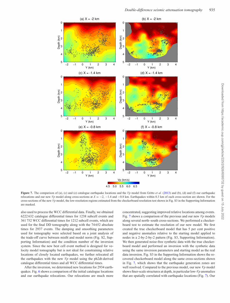
Figure 7. The comparison of (a), (c) and (e) catalogue earthquake locations and the Vp model from Gritto et al. (2013) and (b), (d) and (f) our earthquakerelocations and our new Vp model along cross-sections at X = −2, −1.4 and −0.8 km. Earthquakes within 0.3 km of each cross-section are shown. For thecross-sections of the new Vp model, the low-resolution regions estimated from the checkerboard resolution test shown in Fig. S3 in the Supporting Informationare masked.
also used to process the WCC differential data. Finally, we obtained6222 632 catalogue differential times for 1238 subcell events and361 752 WCC differential times for 1212 subcell events, which areused for the final DD tomography along with the 74 652 absolutetimes for 2937 events. The damping and smoothing parametersused for tomography were selected based on a joint analysis ofthe trade-off curve between misfit and model norm (Fig. S2, Sup-porting Information) and the condition number of the inversionsystem. Since the new best cell event method is designed for ve-locity model tomography but is not ideal for constraining relativelocations of closely located earthquakes, we further relocated allthe earthquakes with the new Vp model using the ph2dt-derivedcatalogue differential times and all WCC differential times.
After the inversion, we determined new locations for 2934 earth-quakes. Fig. 6 shows a comparison of the initial catalogue locationsand our earthquake relocations. Our relocations are much more
concentrated, suggesting improved relative locations among events.Fig. 7 shows a comparison of the previous and our new Vp modelsalong several north–south cross-sections. We performed a checker-board test to estimate the resolution of our new model. We firstcreated the true checkerboard model that has 5 per cent positiveand negative anomalies relative to the starting model applied tonodes in a 2-by-2-by-2 pattern (Fig. S3, Supporting Information).We then generated noise-free synthetic data with the true checker-board model and performed an inversion with the synthetic datausing the same inversion parameters and starting model as the realdata inversion. Fig. S3 in the Supporting Information shows the re-covered checkerboard model along the same cross-sections shownin Fig. 7, which shows that the earthquake generation zones arewell resolved. Compared to the previous model, our new Vp modelshows finer-scale structures at depth, in particular low-Vp anomaliesthat are spatially correlated with earthquake locations (Fig. 7). Our
Dow
nloaded from https://academ
ic.oup.com/gji/article/225/2/926/6095732 by guest on 15 July 2022
936 H. Guo and C. Thurber
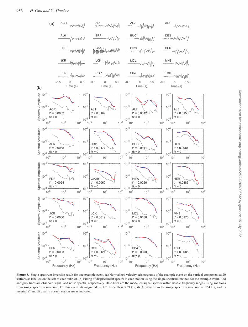
Figure 8. Single spectrum inversion result for one example event. (a) Normalized velocity seismograms of the example event on the vertical component at 20stations as labelled on the left of each subplot. (b) Fitting of displacement spectra at each station using the single spectrum method for the example event. Redand grey lines are observed signal and noise spectra, respectively. Blue lines are the modelled signal spectra within usable frequency ranges using solutionsfrom single spectrum inversion. For this event, its magnitude is 1.7, its depth is 3.59 km, its fc value from the single spectrum inversion is 12.4 Hz, and itsinverted t∗ and fit quality at each station are as indicated.
Dow
nloaded from https://academ
ic.oup.com/gji/article/225/2/926/6095732 by guest on 15 July 2022
Double-difference seismic attenuation tomography 937
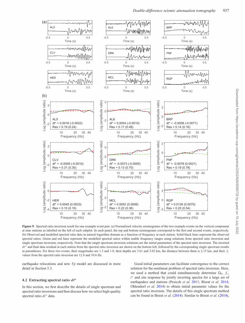
Figure 9. Spectral ratio inversion result for one example event pair. (a) Normalized velocity seismograms of the two example events on the vertical componentat nine stations as labelled on the left of each subplot. In each panel, the top and bottom seismograms correspond to the first and second events, respectively.(b) Observed and modelled spectral ratio data in natural logarithm domain as a function of frequency at each station. Solid black lines represent the observedspectral ratios. Green and red lines represent the modelled spectral ratios within usable frequency ranges using solutions from spectral ratio inversion andsingle spectrum inversion, respectively. Note that the single spectrum inversion solutions are the initial parameters of the spectral ratio inversion. The inverteddt∗ and final data residual at each station from the spectral ratio inversion are shown on the bottom left, followed by the corresponding single spectrum resultsin parentheses. For these two events, their magnitudes are 1.3 and 1.0, their depths are 3.61 and 3.02 km, the distance between them is 2.15 km, and their fc
values from the spectral ratio inversion are 12.8 and 10.6 Hz.
earthquake relocations and new Vp model are discussed in moredetail in Section 5.3.
4.2 Extracting spectral ratio dt∗
In this section, we first describe the details of single spectrum andspectral ratio inversions and then discuss how we select high-qualityspectral ratio dt∗ data.
Good initial parameters can facilitate convergence to the correctsolution for the nonlinear problem of spectral ratio inversion. Here,we used a method that could simultaneously determine �0, fc,t∗ and site response by jointly inverting spectra for a large set ofearthquakes and stations (Pesicek et al. 2011; Bisrat et al. 2014;Ohlendorf et al. 2014) to obtain initial parameter values for thespectral ratio inversion. The details of this single spectrum methodcan be found in Bisrat et al. (2014). Similar to Bisrat et al. (2014),
Dow
nloaded from https://academ
ic.oup.com/gji/article/225/2/926/6095732 by guest on 15 July 2022
938 H. Guo and C. Thurber
Figure 10. Histograms of initial (light grey) and final (dark grey) spectralratio residuals (a) for each event pair and (b) for each individual observation.
a series of criteria were designed to process the raw waveformdata and select the ones that can be used for the single spectruminversion and the subsequent spectral ratio inversion. All verticalcomponent waveforms were first processed by removing the meanand linear trend. We then calculated signal spectra from 1.024 stime windows around P-wave arrivals (0.424 s before the arrival and0.6 s after the arrival) and noise spectra from 1.024 s time windowsbefore the signal windows using a multitaper spectrum estimationmethod (Thomson 1982) with a frequency range of 1.67–50 Hz.To avoid contamination of P-wave signals by S-wave signals, onlywaveforms with an S–P arrival time difference above 0.7 s wereused. The calculated spectra were then smoothed with a 3-point-long moving window. SNRs were then calculated for all spectra.The signal spectra were selected for the single spectrum inversionif the SNR was above a threshold of 2.5 in a continuous frequencyrange of at least 10 Hz. After the single spectrum inversion, theobtained t∗ solutions were assigned quality values 0 (best) to 4(worst) based on the fit between the observed and predicted spectra.After the single spectrum inversion with data from 2962 events, weobtained 54 611 t∗ values of quality of 0, 1 and 2, which were usedas the initial parameters for the subsequent spectral ratio inversion.The single spectrum inversion result for one example event is shownin Fig. 8.
For the spectral ratio inversion, the data pre-processing stepsare the same as that used for the single spectrum inversion. Afterobtaining the individual spectra and the corresponding SNRs, wecalculated spectral ratios for each event pair with an inter-eventdistance less than 3 km if the SNRs of both spectra were above 3within a common and continuous frequency range of at least 10 Hz.The calculated spectral ratios were smoothed with a 5-point-longmoving window and then used for the spectral ratio inversion. Afterthe inversion using a frequency range of 1.67–50 Hz, we found that,overall, the frequency range below ∼5 Hz had larger misfit thanhigher frequencies, therefore we modified the frequency range to5–50 Hz for the final inversion. For the damping parameter λ, wesearched for a value that could constrain the condition number ofthe inversion system to be ∼10. Overall, the resulting resolutionvalues of all parameters for all spectral ratio inversions using theselected λ values are around 0.5. We stopped the iterations when therms spectral ratio misfit did not change significantly or reached the
predetermined maximum number of iterations (20). Overall, mostinversions converged very quickly after 1–3 iterations.
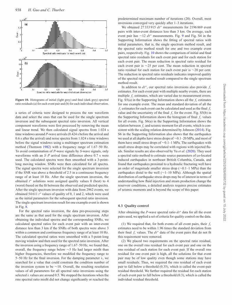
We obtained 27 333 915 dt∗ measurements for 2196 869 eventpairs with inter-event distances less than 3 km. On average, eachevent pair has ∼12 dt∗ measurements. Fig. 9 and Fig. S4 in theSupporting Information shows the fitting of spectral ratios withinitial parameters, that is, the single spectrum method result, andthe spectral ratio method result for one and two example eventpairs, respectively. Fig. 10 shows the comparison of initial and finalspectral ratio residuals for each event pair and for each station foreach event pair. The mean reduction in spectral ratio residual foreach event pair is ∼25 per cent. The mean reduction in spectralratio residual for each station for each event pair is ∼20 per cent.The reduction in spectral ratio residuals indicates improved qualityof the spectral ratio method result compared to the single spectrummethod result.
In addition to dt∗, our spectral ratio inversions also provide fc
estimates. For each event pair with multiple nearby events, there aremultiple fc estimates, which are varied due to measurement errors.Fig. S5(a) in the Supporting Information shows all the fc estimatesfor one example event. The mean and standard deviation of all thefc estimates for each event can be calculated and used as the final fc
value and the uncertainty of the final fc for the event. Fig. S5(b) inthe Supporting Information shows the histogram of final fc valuesfor all events. Fig. S6(a) in the Supporting Information shows therelation between fc and seismic moment for all events, which is con-sistent with the scaling relation determined by Johnson (2014). Fig.S6 in the Supporting Information also shows that the earthquakeswe used at all depths have stress drops of ∼0.1–20 MPa, and most ofthem have small stress drops of ∼0.1–1 MPa. The earthquakes withsmall stress drops may be correlated with regions with injected flu-ids. Similar results are also observed by Yu et al. (2020). They useda spectral ratio method to estimate source parameters of co-locatedinduced earthquakes in northeast British Columbia, Canada, andfound that earthquakes proximal to a hydraulic fracturing well havean order of magnitude smaller stress drop (∼0.1–1 MPa) than theearthquakes distal to the well (∼1–10 MPa). Although the spatialdistribution of earthquake stress drops may be of interest in terms ofunderstanding how fluid injection and steam production change thereservoir conditions, a detailed analysis requires precise estimatesof seismic moments and is beyond the scope of this paper.
4.3 Quality control
After obtaining the P-wave spectral ratio dt∗ data for all the eventpairs used, we applied a set of criteria for quality control on the data.
(1) We required that, for both events of all event pairs, their fc
estimates need to be within 1.96 times the standard deviation fromtheir final fc values. The dt∗ data of the event pairs that do not fitthis requirement were removed.
(2) We placed two requirements on the spectral ratio residual,one on the overall rms residual for each event pair and one on therms residual of each station for each event pair. If the overall rmsresidual for one event pair is high, all the solutions for that eventpair may be of low quality even though some stations may havesmall residuals. Thus, we required the rms residual of each eventpair to fall below a threshold (0.35), which is called the event-pairresidual threshold. We further required the residual for each stationof each event pair to fall below a threshold (0.3), which is called theindividual residual threshold.
Dow
nloaded from https://academ
ic.oup.com/gji/article/225/2/926/6095732 by guest on 15 July 2022
Double-difference seismic attenuation tomography 939
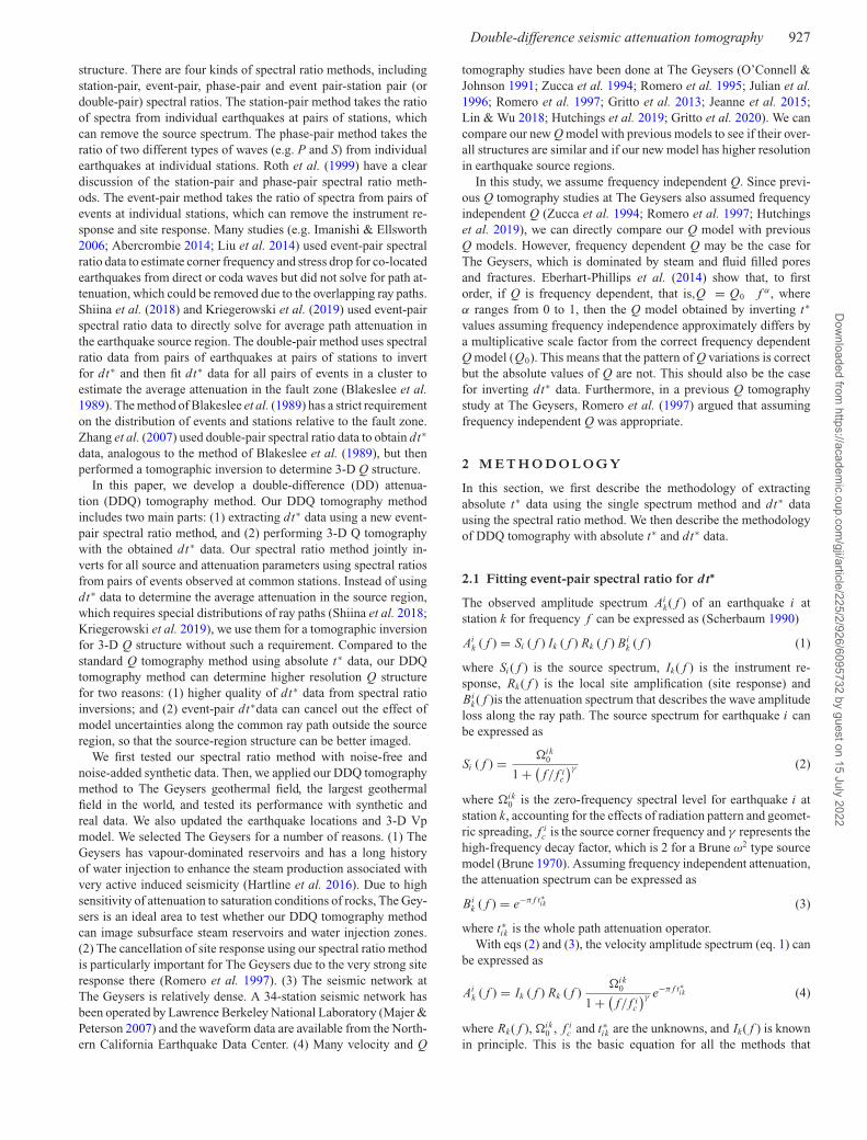
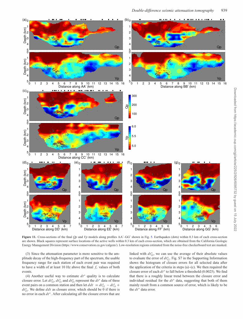
Figure 11. Cross-sections of the final Qp and Vp models along profiles AA′–GG′ shown in Fig. 5. Earthquakes (dots) within 0.3 km of each cross-sectionare shown. Black squares represent surface locations of the active wells within 0.3 km of each cross-section, which are obtained from the California GeologicEnergy Management Division (https://www.conservation.ca.gov/calgem/). Low-resolution regions estimated from the noise-free checkerboard test are masked.
(3) Since the attenuation parameter is more sensitive to the am-plitude decay of the high-frequency part of the spectrum, the usablefrequency range for each station of each event pair was requiredto have a width of at least 10 Hz above the final fc values of bothevents.
(4) Another useful way to estimate dt∗ quality is to calculateclosure error. Let dt∗
12, dt∗13 and dt∗
23 represent the dt∗ data of threeevent pairs on a common station and then let ddt = dt∗
12 − dt∗13 +
dt∗23. We define ddt as closure error, which should be 0 if there is
no error in each dt∗. After calculating all the closure errors that are
linked with dt∗12, we can use the average of their absolute values
to evaluate the error of dt∗12. Fig. S7 in the Supporting Information
shows the histogram of closure errors for all selected data afterthe application of the criteria in steps (a)–(c). We then required theclosure error of each dt∗ to fall below a threshold (0.0025). We findthat there is a roughly linear trend between the closure error andindividual residual for the dt∗ data, suggesting that both of themmainly result from a common source of error, which is likely to bethe dt∗ data error.
Dow
nloaded from https://academ
ic.oup.com/gji/article/225/2/926/6095732 by guest on 15 July 2022
940 H. Guo and C. Thurber
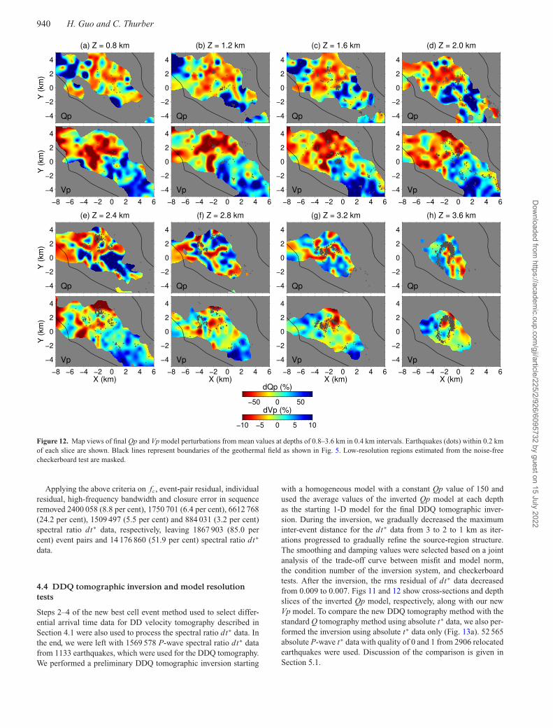
Figure 12. Map views of final Qp and Vp model perturbations from mean values at depths of 0.8–3.6 km in 0.4 km intervals. Earthquakes (dots) within 0.2 kmof each slice are shown. Black lines represent boundaries of the geothermal field as shown in Fig. 5. Low-resolution regions estimated from the noise-freecheckerboard test are masked.
Applying the above criteria on fc, event-pair residual, individualresidual, high-frequency bandwidth and closure error in sequenceremoved 2400 058 (8.8 per cent), 1750 701 (6.4 per cent), 6612 768(24.2 per cent), 1509 497 (5.5 per cent) and 884 031 (3.2 per cent)spectral ratio dt∗ data, respectively, leaving 1867 903 (85.0 percent) event pairs and 14 176 860 (51.9 per cent) spectral ratio dt∗
data.
4.4 DDQ tomographic inversion and model resolutiontests
Steps 2–4 of the new best cell event method used to select differ-ential arrival time data for DD velocity tomography described inSection 4.1 were also used to process the spectral ratio dt∗ data. Inthe end, we were left with 1569 578 P-wave spectral ratio dt∗ datafrom 1133 earthquakes, which were used for the DDQ tomography.We performed a preliminary DDQ tomographic inversion starting
with a homogeneous model with a constant Qp value of 150 andused the average values of the inverted Qp model at each depthas the starting 1-D model for the final DDQ tomographic inver-sion. During the inversion, we gradually decreased the maximuminter-event distance for the dt∗ data from 3 to 2 to 1 km as iter-ations progressed to gradually refine the source-region structure.The smoothing and damping values were selected based on a jointanalysis of the trade-off curve between misfit and model norm,the condition number of the inversion system, and checkerboardtests. After the inversion, the rms residual of dt∗ data decreasedfrom 0.009 to 0.007. Figs 11 and 12 show cross-sections and depthslices of the inverted Qp model, respectively, along with our newVp model. To compare the new DDQ tomography method with thestandard Q tomography method using absolute t∗ data, we also per-formed the inversion using absolute t∗ data only (Fig. 13a). 52 565absolute P-wave t∗ data with quality of 0 and 1 from 2906 relocatedearthquakes were used. Discussion of the comparison is given inSection 5.1.
Dow
nloaded from https://academ
ic.oup.com/gji/article/225/2/926/6095732 by guest on 15 July 2022
Double-difference seismic attenuation tomography 941
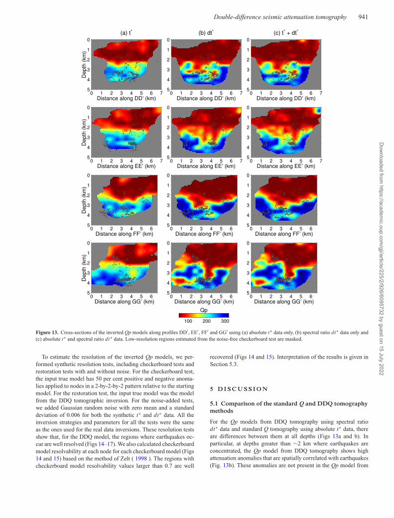
Figure 13. Cross-sections of the inverted Qp models along profiles DD′, EE′, FF′ and GG′ using (a) absolute t∗ data only, (b) spectral ratio dt∗ data only and(c) absolute t∗ and spectral ratio dt∗ data. Low-resolution regions estimated from the noise-free checkerboard test are masked.
To estimate the resolution of the inverted Qp models, we per-formed synthetic resolution tests, including checkerboard tests andrestoration tests with and without noise. For the checkerboard test,the input true model has 50 per cent positive and negative anoma-lies applied to nodes in a 2-by-2-by-2 pattern relative to the startingmodel. For the restoration test, the input true model was the modelfrom the DDQ tomographic inversion. For the noise-added tests,we added Gaussian random noise with zero mean and a standarddeviation of 0.006 for both the synthetic t∗ and dt∗ data. All theinversion strategies and parameters for all the tests were the sameas the ones used for the real data inversions. These resolution testsshow that, for the DDQ model, the regions where earthquakes oc-cur are well resolved (Figs 14–17). We also calculated checkerboardmodel resolvability at each node for each checkerboard model (Figs14 and 15) based on the method of Zelt ( 1998 ). The regions withcheckerboard model resolvability values larger than 0.7 are well
recovered (Figs 14 and 15). Interpretation of the results is given inSection 5.3.
5 D I S C U S S I O N
5.1 Comparison of the standard Q and DDQ tomographymethods
For the Qp models from DDQ tomography using spectral ratiodt∗ data and standard Q tomography using absolute t∗ data, thereare differences between them at all depths (Figs 13a and b). Inparticular, at depths greater than ∼2 km where earthquakes areconcentrated, the Qp model from DDQ tomography shows highattenuation anomalies that are spatially correlated with earthquakes(Fig. 13b). These anomalies are not present in the Qp model from
Dow
nloaded from https://academ
ic.oup.com/gji/article/225/2/926/6095732 by guest on 15 July 2022

942 H. Guo and C. Thurber
Figure 14. Cross-sections of the (a) input true and (b)–(d) inverted Qp models from noise-free checkerboard tests using (b) absolute t∗ data only, (c) dt∗ dataonly and (d) absolute t∗ and dt∗ data. Black curves represent the contour of checkerboard model resolvability of 0.7. Dots represent earthquakes within 0.3 kmof each cross-section.
standard Q tomography (Fig. 13a). Both the noise-free (Figs 14band c and 16b and c) and noise-added (Figs 15b and c and 17b andc) checkerboard and restoration tests show that the dt∗ inversioncan better recover the true model than the t∗ inversion, especially
in earthquake source regions. These results clearly indicate that thenew DDQ tomography method using spectral ratio dt∗ data candetermine higher resolution attenuation structure than the standardmethod using t∗ data.
Dow
nloaded from https://academ
ic.oup.com/gji/article/225/2/926/6095732 by guest on 15 July 2022
Double-difference seismic attenuation tomography 943
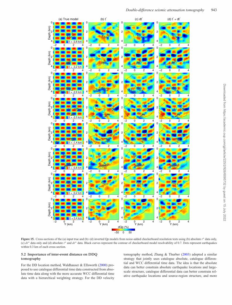
Figure 15. Cross-sections of the (a) input true and (b)–(d) inverted Qp models from noise-added checkerboard resolution tests using (b) absolute t∗ data only,(c) dt∗ data only and (d) absolute t∗ and dt∗ data. Black curves represent the contour of checkerboard model resolvability of 0.7. Dots represent earthquakeswithin 0.3 km of each cross-section.
5.2 Importance of inter-event distance on DDQtomography
For the DD location method, Waldhauser & Ellsworth (2000) pro-posed to use catalogue differential time data constructed from abso-lute time data along with the more accurate WCC differential timedata with a hierarchical weighting strategy. For the DD velocity
tomography method, Zhang & Thurber (2003) adopted a similarstrategy that jointly uses catalogue absolute, catalogue differen-tial and WCC differential time data. The idea is that the absolutedata can better constrain absolute earthquake locations and large-scale structure, catalogue differential data can better constrain rel-ative earthquake locations and source-region structure, and more
Dow
nloaded from https://academ
ic.oup.com/gji/article/225/2/926/6095732 by guest on 15 July 2022
944 H. Guo and C. Thurber
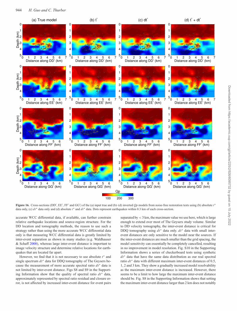
Figure 16. Cross-sections (DD′, EE′, FF′ and GG′) of the (a) input true and (b)–(d) inverted Qp models from noise-free restoration tests using (b) absolute t∗data only, (c) dt∗ data only and (d) absolute t∗ and dt∗ data. Dots represent earthquakes within 0.3 km of each cross-section.
accurate WCC differential data, if available, can further constrainrelative earthquake locations and source-region structure. For theDD location and tomography methods, the reason to use such astrategy rather than using the more accurate WCC differential dataonly is that measuring WCC differential data is greatly limited byinter-event separation as shown in many studies (e.g. Waldhauser& Schaff 2008), whereas large inter-event distance is important toimage velocity structure and determine relative locations for earth-quakes that are located far apart.
However, we find that it is not necessary to use absolute t∗ andsingle spectrum dt∗ data for DDQ tomography of The Geysers be-cause the measurement of more accurate spectral ratio dt∗ data isnot limited by inter-event distance. Figs S8 and S9 in the Support-ing Information show that the quality of spectral ratio dt∗ data,approximately represented by spectral ratio residual and closure er-ror, is not affected by increased inter-event distance for event pairs
separated by < 3 km, the maximum value we use here, which is largeenough to extend over most of The Geysers study volume. Similarto DD velocity tomography, the inter-event distance is critical forDDQ tomography using dt∗ data only. dt∗ data with small inter-event distances are only sensitive to the model near the sources. Ifthe inter-event distances are much smaller than the grid spacing, themodel sensitivity can essentially be completely cancelled, resultingin no improvement in model resolution. Fig. S10 in the SupportingInformation shows a series of checkerboard tests using syntheticdt∗ data that have the same data distribution as our real spectralratio dt∗ data with different maximum inter-event distances of 0.5,1, 2 and 3 km. They show a gradually increased model resolvabilityas the maximum inter-event distance is increased. However, thereseems to be a limit to how large the maximum inter-event distanceshould be. Fig. S8 in the Supporting Information shows that settingthe maximum inter-event distance larger than 2 km does not notably
Dow
nloaded from https://academ
ic.oup.com/gji/article/225/2/926/6095732 by guest on 15 July 2022
Double-difference seismic attenuation tomography 945
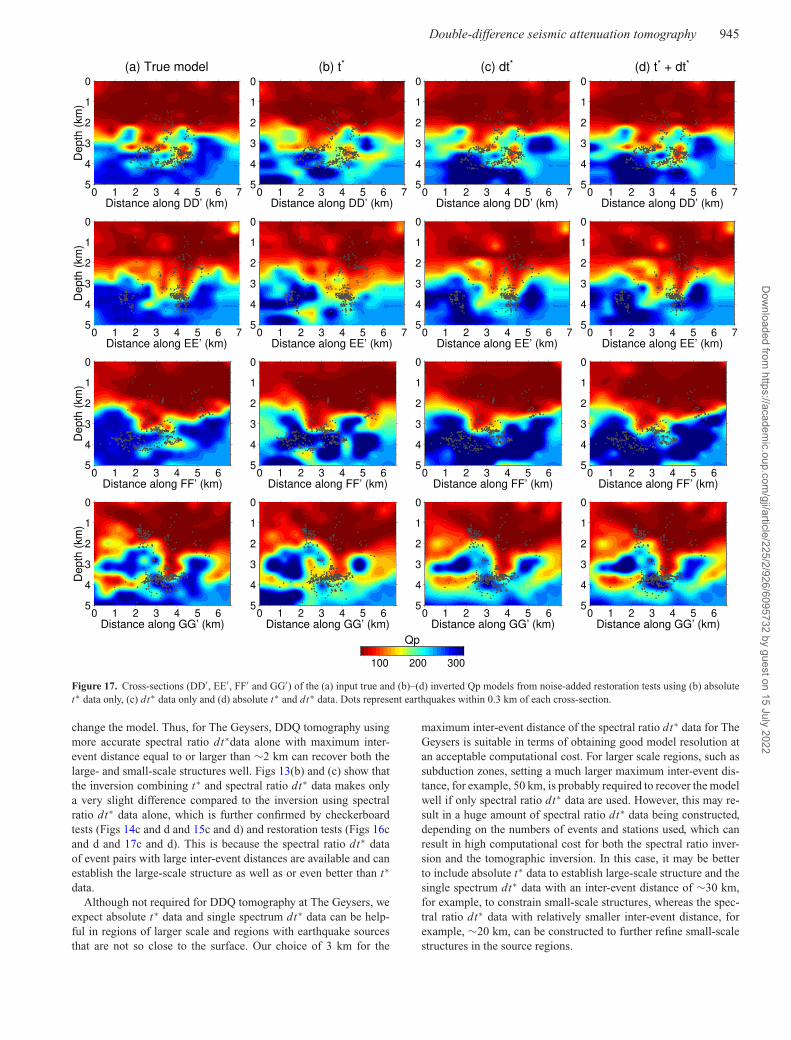
Figure 17. Cross-sections (DD′, EE′, FF′ and GG′) of the (a) input true and (b)–(d) inverted Qp models from noise-added restoration tests using (b) absolutet∗ data only, (c) dt∗ data only and (d) absolute t∗ and dt∗ data. Dots represent earthquakes within 0.3 km of each cross-section.
change the model. Thus, for The Geysers, DDQ tomography usingmore accurate spectral ratio dt∗data alone with maximum inter-event distance equal to or larger than ∼2 km can recover both thelarge- and small-scale structures well. Figs 13(b) and (c) show thatthe inversion combining t∗ and spectral ratio dt∗ data makes onlya very slight difference compared to the inversion using spectralratio dt∗ data alone, which is further confirmed by checkerboardtests (Figs 14c and d and 15c and d) and restoration tests (Figs 16cand d and 17c and d). This is because the spectral ratio dt∗ dataof event pairs with large inter-event distances are available and canestablish the large-scale structure as well as or even better than t∗
data.Although not required for DDQ tomography at The Geysers, we
expect absolute t∗ data and single spectrum dt∗ data can be help-ful in regions of larger scale and regions with earthquake sourcesthat are not so close to the surface. Our choice of 3 km for the
maximum inter-event distance of the spectral ratio dt∗ data for TheGeysers is suitable in terms of obtaining good model resolution atan acceptable computational cost. For larger scale regions, such assubduction zones, setting a much larger maximum inter-event dis-tance, for example, 50 km, is probably required to recover the modelwell if only spectral ratio dt∗ data are used. However, this may re-sult in a huge amount of spectral ratio dt∗ data being constructed,depending on the numbers of events and stations used, which canresult in high computational cost for both the spectral ratio inver-sion and the tomographic inversion. In this case, it may be betterto include absolute t∗ data to establish large-scale structure and thesingle spectrum dt∗ data with an inter-event distance of ∼30 km,for example, to constrain small-scale structures, whereas the spec-tral ratio dt∗ data with relatively smaller inter-event distance, forexample, ∼20 km, can be constructed to further refine small-scalestructures in the source regions.
Dow
nloaded from https://academ
ic.oup.com/gji/article/225/2/926/6095732 by guest on 15 July 2022
946 H. Guo and C. Thurber
5.3 Interpretation of reservoir conditions of The Geysers
We divide the whole geothermal field of The Geysers into threeregions. The northwest region is to the northwest of a line trend-ing northeast passing through the point X = 0 km and Y = 0 km(horizontal distances < ∼7 km in the AA′–CC′ cross-sections inFigs 11a and c). The central region is between two lines trendingnortheast passing through two points, one of which is X = 0 km andY = 0 km, and the other one is X = −2 km and Y = −2 km (horizon-tal distances ∼7–10 km in the AA′–CC′ cross-sections in Figs 11aand c). The southeast region is to the southeast of the line trendingnortheast passing through the point X = −2 km and Y = −2 km(horizontal distances > ∼10 km in the AA′–CC′ cross-sections inFigs 11a and c). Note that depth throughout the paper is definedrelative to sea level.
Strong lateral and vertical heterogeneity of the reservoir condi-tions have been found beneath the entirety of The Geyser geothermalfield by many previous geophysics, geology, geochemistry, hydrol-ogy, rock physics and mechanical modelling studies in the pastdecades (Walters et al. 1988; O’Connell & Johnson 1991; Zuccaet al. 1994; Romero et al. 1995; Julian et al. 1996; Romero et al.1997; Gritto et al. 2013; Garcia et al. 2016; Rutqvist et al. 2016;Lin & Wu 2018; Hutchings et al. 2019). In recent years, more at-tention has been paid to the northwest region, where a deep vapour-dominated high temperature reservoir (HTR, ∼300–400 ◦C) existsat depths below ∼2 km underneath a conventional steam reservoir ofnormal temperature (NTR, ∼240 ◦C) at depths of ∼1–2 km (Walteret al. 1988). An Enhanced Geothermal System (EGS) Demonstra-tion Project has been performed in this area since 2009 (Jeanneet al. 2015; Garcia et al. 2016; Rutqvist et al. 2016), which aimsto enhance the production from the HTR by water injection. Previ-ous seismic velocity and attenuation tomography studies show lowVp/Vs and high attenuation anomalies at depths of ∼2–3 km in thenorthwest region, which may correspond to the HTR (e.g. Romeroet al. 1995,1997; Julian et al. 1996; Lin & Wu 2018). Due to limitedresolution at the depth of the HTR, however, it has not been wellresolved by seismic tomography studies in terms of its depth rangeand lateral extent. The Geysers has a long history of water injectionto enhance the steam production from the NTR and HTR (Hartlineet al. 2016). High-resolution imaging of structure of water injec-tion zones is important to understand how the injection activitieshave changed the reservoir conditions (Jeanne et al. 2015). Here,we focus on using our high-resolution earthquake relocations, Vpand Qp models to characterize the NTR, HTR and water injectionzone.
The NTR extends throughout the geothermal field with varyingdepth range in different regions, whereas the HTR only exists inthe northwest region. Northwest–southeast cross-sections and hor-izontal slices of the Vp and Qp models show that, at depths of∼0.5–2 km where the NTR is located, both Vp and Qp are lowest inthe southeastern part of the northwest region (Figs 11a–c and 12a–d). This zone has also been imaged as a low Vp and low Vp/Vs(1.67–1.72) zone by previous tomography studies (e.g. Julian et al.1996; Lin & Wu 2018). At ∼2 km depth, there is a generally sharptransition in Vp and Qp beneath the northwest region, which can beseen from all cross-sections of different orientations crossing thisregion (Fig. 11). This transition well characterizes the boundary be-tween the NTR and HTR. Below ∼2 km depth, the most prominentstructure is a ∼1–2 km wide zone of low Vp and Qp in the HTR inthe southeastern part of the northwest region (horizontal distances∼4–6 km in Figs 11a–c), associated with very active seismicity.Earthquakes are relatively scattered in its upper portion, but are very
concentrated and show lineations in its lower portion. The bottomof this anomaly extends to nearby regions in some cross-sections.Southwest–northeast cross-sections and north–south cross-sectionsalso clearly show this anomaly at depths of ∼2–4 km (Figs 11d–g).Compared to this anomaly, the region further to the northwest (hor-izontal distances < ∼4 km in Figs 11a–c) shows relatively higherVp and Qp. Fig. 12 shows the depth slices of the Vp and Qp modelsrelative to the mean values at each depth, which better shows thelateral extent of the anomalies seen from the cross-sections. Overall,Vp and Qp at each depth vary horizontally from the northwest to thesoutheast regions by ±10 per cent and ±60 per cent, respectively,with lowest Vp and Qp in the southeastern part of the northwestregion. The sharp contrast in Vp and Qp between the northwest andthe central regions at depths less than ∼2 km may indicate the deepextension of a local northeast-trending fault into the NTR depthrange (Garcia et al. 2016).
Factors that influence Vp, Qp and other physical properties in thecrust include lithology, fracturing, fluid versus gas saturation, effec-tive pressure, temperature and hydration of minerals, especially forsteam reservoirs in geothermal fields. The Geysers steam reservoirslie primarily within a metagraywacke and are overlain by Franciscangreenstone melange and unfractured metagraywacke (Thompson1992). A felsite body intruded into the base of the metagraywackeduring the Pleistocene (Schriener & Suemnicht 1980) and it is sug-gested to have hydrothermally altered and hydraulically fracturedthe metagraywacke, increasing the permeability to host the presentsteam reservoirs (Romero et al. 1995). Combined with a long his-tory of fluid injection since 1970 to sustain or enhance the reservoirpressure and the steam production, the NTR and HTR are highlyfractured, with fractures filled by liquid and/or vapour (Hartlineet al. 2016).
Our observed variations in Vp and Qp in the NTR throughout thefield are too large to be the effect of temperature variation aloneand must be explained by variations in fracturing, pore pressure,permeability, saturation and/or lithology (Julian et al. 1996). Thesefactors have been thoroughly investigated by theoretical and labrock physics studies (e.g. Winkler & Nur 1979; Hutchings et al.2019). Two important activities, water injection and steam produc-tion, are likely responsible for these variations. Since the geothermalreservoir is naturally vapour-dominated, low Vp/Vs is expected aswas imaged by Julian et al. (1996). In the southeastern part of thenorthwest region, the distribution of wells is denser than any otherpart of the field (Fig. 11). In high porosity rocks, the introduction offluids into pores or fractures from the water injection activities canincrease the rock density and decrease Vp, although bulk modulusis increased. Partial saturation of fluids also increases intrinsic at-tenuation. Water injection can also result in more fracturing that de-creases Vp due to the decreased bulk modulus. More fracturing alsoincreases intrinsic attenuation. As steam is produced continuously,steam pressure in the reservoir is decreased and thus effective stressis increased. This can result in increased velocity and decreasedattenuation. Since the injected fluid can be converted to steam afterencountering hot reservoir rocks, however, steam pressure can berecovered to some degree. Thus, we suggest two possible interpreta-tions for the large northwest to southeast variations in Vp and Qp inthe NTR. (1) The southeastern part of the northwest region, whereboth Vp and Qp are lowest, has a higher degree of fracturing, per-meability, and saturation (although not fully saturated), comparedto the regions to the southeast and northwest. (2) Steam pressure issignificantly lower in the central and southeast regions due to steamproduction.
Dow
nloaded from https://academ
ic.oup.com/gji/article/225/2/926/6095732 by guest on 15 July 2022
Double-difference seismic attenuation tomography 947
For the HTR in the northwest region, the strong variations in Vpand Qp within it may reflect variations in permeability and satu-ration. For the southeastern part of the HTR (horizontal distances∼4–6 km in AA′–CC′ cross-sections in Figs 11a–c), earthquakesare concentrated at its base. As the cool water encounters hot reser-voir rocks, microearthquakes are induced due to the generationof new cracks and fractures and the reactivation of existing frac-tures (Hartline et al. 2016, and references therein). Consequently,microearthquakes can be used as a proxy for pathways of fluidmigration near the injection wells. Clustered earthquakes in thesoutheastern part of the HTR, some of which show lineations, indi-cate the existence of fluids in this narrow zone, which is probablydue to water injection. Our imaged low Vp and extremely low Qpof this narrow zone probably indicates very high partial fluid sat-uration there, perhaps up to ∼ 95 per cent (Winkler & Nur 1979).This is consistent with the fact that since 2003 November, the SantaRosa—Geysers Recharge Project has injected a large amount oftertiary-treated wastewater into this region (Stark et al. 2005; Majer& Peterson 2007). Another tomography study also shows that Vpis decreased at ∼2–3 km depths after the water injection duringan EGS Demonstration Project near the northwestern edge of ourstudy area (Jeanne et al. 2015). For the northwestern part of theHTR (horizontal distances < ∼4 km in AA′–CC′ cross-sections inFigs 11a–c), Vp and Qp are relatively higher, indicating much lessfluid saturation or even dry fractures there (Winkler & Nur 1979).This is consistent with the inference of hot dry rocks in the HTR(Walters et al. 1988; Garcia et al. 2016).
6 C O N C LU S I O N S
We have developed an event-pair spectral ratio method that cansolve for source and attenuation parameters using spectral ratio datafrom pairs of events at common stations. By taking the ratio, boththe instrument and site responses are removed from the inversion.Synthetic tests show that the inversion of dt∗ data using our spectralratio method is relatively insensitive to the choice of source model(high-frequency decay factor) and is robust to a moderate amountof noise. Applying the new spectral ratio method to real P-wavedata at The Geysers fits the data better than the standard singlespectrum method, indicating that the spectral ratio dt∗ data aremore accurate than absolute t∗ data. Before DDQ tomographicinversion, we relocated 2937 earthquakes and determined a new3-D Vp model using the DD location and tomography method,with a new strategy for constructing event-pair differential timedata. Both the real data inversions and synthetic tests show thatDDQ tomographic inversion using spectral ratio dt∗ data achieveshigher resolution at The Geysers than the standard Q tomographicinversion using absolute t∗ data, especially in zones of concentratedearthquakes. At depths of ∼0.5–2 km where a vapour-dominatedNTR exists, our results reveal strong variations in Vp and Qp fromthe northwest to the southeast regions, which can be attributed tovariations in fracturing, permeability, fluid saturation and/or steampressure. At depths of ∼2–4 km, a prominent low-Vp and low-Qpzone is imaged within a known HTR and is probably caused bythe large amount of fluids injected into this zone, which can alsoexplain the very active induced seismicity there.
A C K N OW L E D G E M E N T S
Waveform data, metadata, or data products for this study were ac-cessed through the Northern California Earthquake Data Center,
doi:10.7932/NCEDC. We thank Gritto Roland for providing eventlists and Avinash Nayak for archiving waveform data. We thanktwo reviewers for their constructive comments that help us to im-prove this manuscript. This work is supported by NSF award EAR-1724685.
DATA AVA I L A B I L I T Y S TAT E M E N T
Waveform data, metadata, or data products for this studywere accessed through the Northern California Earthquake DataCenter (2014). The earthquake relocations and Vp and Qpmodels developed in this study are available in Zenodo, athttps://zenodo.org/record/4470253#.YBDr1y-ZNVo. The DDQ to-mography code can be made available upon request.
R E F E R E N C E SAbercrombie, R.E., 2014. Stress drops of repeating earthquakes on the San
Andreas fault at Parkfield, Geophys. Res. Lett., 41(24), 8784–8791.Aster, R.C., Borchers, B. & Thurber, C.H., 2019. Parameter Estimation and
Inverse Problems, Academic Press.Bakun , W.H., 1984. Seismic moments, local magnitudes, and coda-duration
magnitudes for earthquakes in central California, Bull. seism. Soc. Am.,74(2):439–458.
Bennington, N., Thurber, C. & Roecker, S., 2008. Three-dimensional seismicattenuation structure around the SAFOD site, Parkfield, California, Bull.seism. Soc. Am., 98(6), 2934–2947.
Bisrat, S.T., DeShon, H.R., Pesicek, J. & Thurber, C., 2014. High-resolution3-DP wave attenuation structure of the New Madrid Seismic Zone usinglocal earthquake tomography, J. geophys. Res.: Solid Earth, 119(1), 409–424.
Blakeslee, S., Malin, P. & Alvarez, M., 1989. Fault-zone attenua-tion of high-frequency seismic waves, Geophys. Res. Lett., 16(11),1321–1324.
Brune, J.N., 1970. Tectonic stress and the spectra of seismic shear wavesfrom earthquakes, J. geophys. Res., 75(26), 4997–5009.
Eberhart-Phillips, D. & Chadwick, M., 2002. Three-dimensional attenu-ation model of the shallow Hikurangi subduction zone in the Rauku-mara Peninsula, New Zealand, J. geophys. Res.: Solid Earth, 107(B2),doi:10.1029/2000JB000046.
Eberhart-Phillips, D., Thurber, C.H. & Fletcher, J.B., 2014. ImagingP and S Attenuation in the Sacramento–San Joaquin Delta Re-gion, Northern California, Bull. seism. Soc. Am., 104(5), 2322–2336,doi:10.1785/0120130336.
Faul, U. & Jackson, I., 2015. Transient creep and strain energy dissipa-tion: an experimental perspective, Annu. Rev. Earth Planet. Sci., 43,541–569.
Frankel, A., 1991. Mechanisms of seismic attenuation in the crust: scatteringand anelasticity in New York State, South Africa, and southern California,J. geophys. Res.: Solid Earth, 96(B4), 6269–6289.
Garcia, J., Hartline, C., Walters, M., Wright, M., Rutqvist, J., Dobson, P.F.& Jeanne, P., 2016. The Northwest Geysers EGS demonstration project,California: Part 1: characterization and reservoir response to injection,Geothermics, 63, 97–119.
Gritto, R. & Jarpe, S.P., 2014. Temporal variations of Vp/Vs-ratio at TheGeysers geothermal field, USA, Geothermics, 52, 112–119.
Gritto, R., Jarpe, S.P., Hutchings, L.J., Ulrich, C., Layland-Bachmann, C.E.,Schoenball, M. & Nakagawa, S., 2020. Seismic imaging of spatial hetero-geneity at The Geysers geothermal reservoir using a cost-effective denseseismic network, in Proceedings, 45th Workshop on Geothermal Reser-voir Engineering, SGP-TR-216, Stanford Geothermal Program, StanfordUniversity, Stanford, California.
Gritto, R., Yoo, S.H. & Jarpe, S.P., 2013. Three-dimensional seismic tomog-raphy at The Geysers geothermal field, CA, USA, in Proceedings, 38thWorkshop on Geothermal Reservoir Engineering, SGP-TR-198, StanfordGeothermal Program, Stanford University, Stanford, California.
Dow
nloaded from https://academ
ic.oup.com/gji/article/225/2/926/6095732 by guest on 15 July 2022
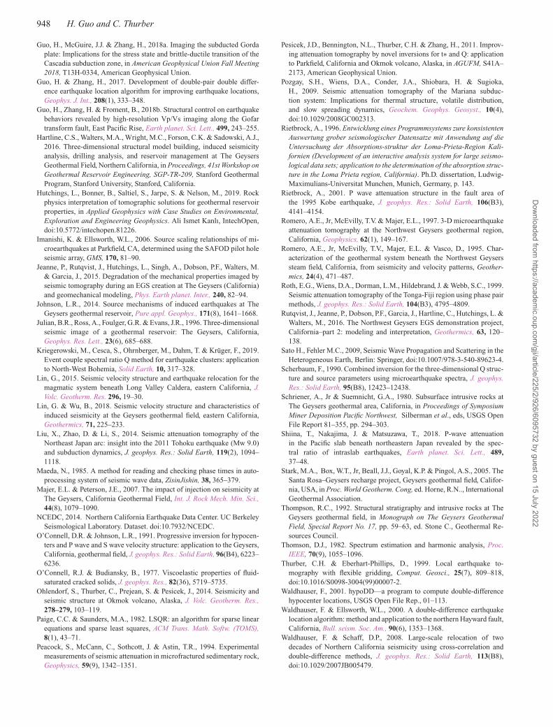
948 H. Guo and C. Thurber
Guo, H., McGuire, J.J. & Zhang, H., 2018a. Imaging the subducted Gordaplate: Implications for the stress state and brittle-ductile transition of theCascadia subduction zone, in American Geophysical Union Fall Meeting2018, T13H-0334, American Geophysical Union.
Guo, H. & Zhang, H., 2017. Development of double-pair double differ-ence earthquake location algorithm for improving earthquake locations,Geophys. J. Int., 208(1), 333–348.
Guo, H., Zhang, H. & Froment, B., 2018b. Structural control on earthquakebehaviors revealed by high-resolution Vp/Vs imaging along the Gofartransform fault, East Pacific Rise, Earth planet. Sci. Lett., 499, 243–255.
Hartline, C.S., Walters, M.A., Wright, M.C., Forson, C.K. & Sadowski, A.J.,2016. Three-dimensional structural model building, induced seismicityanalysis, drilling analysis, and reservoir management at The GeysersGeothermal Field, Northern California, in Proceedings, 41st Workshop onGeothermal Reservoir Engineering, SGP-TR-209, Stanford GeothermalProgram, Stanford University, Stanford, California.
Hutchings, L., Bonner, B., Saltiel, S., Jarpe, S. & Nelson, M., 2019. Rockphysics interpretation of tomographic solutions for geothermal reservoirproperties, in Applied Geophysics with Case Studies on Environmental,Exploration and Engineering Geophysics. Ali Ismet Kanlı, IntechOpen,doi:10.5772/intechopen.81226.
Imanishi, K. & Ellsworth, W.L., 2006. Source scaling relationships of mi-croearthquakes at Parkfield, CA, determined using the SAFOD pilot holeseismic array, GMS, 170, 81–90.
Jeanne, P., Rutqvist, J., Hutchings, L., Singh, A., Dobson, P.F., Walters, M.& Garcia, J., 2015. Degradation of the mechanical properties imaged byseismic tomography during an EGS creation at The Geysers (California)and geomechanical modeling, Phys. Earth planet. Inter., 240, 82–94.
Johnson, L.R., 2014. Source mechanisms of induced earthquakes at TheGeysers geothermal reservoir, Pure appl. Geophys., 171(8), 1641–1668.
Julian, B.R., Ross, A., Foulger, G.R. & Evans, J.R., 1996. Three-dimensionalseismic image of a geothermal reservoir: The Geysers, California,Geophys. Res. Lett., 23(6), 685–688.
Kriegerowski, M., Cesca, S., Ohrnberger, M., Dahm, T. & Kruger, F., 2019.Event couple spectral ratio Q method for earthquake clusters: applicationto North-West Bohemia, Solid Earth, 10, 317–328.
Lin, G., 2015. Seismic velocity structure and earthquake relocation for themagmatic system beneath Long Valley Caldera, eastern California, J.Volc. Geotherm. Res. 296, 19–30.
Lin, G. & Wu, B., 2018. Seismic velocity structure and characteristics ofinduced seismicity at the Geysers geothermal field, eastern California,Geothermics, 71, 225–233.
Liu, X., Zhao, D. & Li, S., 2014. Seismic attenuation tomography of theNortheast Japan arc: insight into the 2011 Tohoku earthquake (Mw 9.0)and subduction dynamics, J. geophys. Res.: Solid Earth, 119(2), 1094–1118.
Maeda, N., 1985. A method for reading and checking phase times in auto-processing system of seismic wave data, ZisinJishin, 38, 365–379.
Majer, E.L. & Peterson, J.E., 2007. The impact of injection on seismicity atThe Geysers, California Geothermal Field, Int. J. Rock Mech. Min. Sci.,44(8), 1079–1090.
NCEDC, 2014. Northern California Earthquake Data Center. UC BerkeleySeismological Laboratory. Dataset. doi:10.7932/NCEDC.
O’Connell, D.R. & Johnson, L.R., 1991. Progressive inversion for hypocen-ters and P wave and S wave velocity structure: application to the Geysers,California, geothermal field, J. geophys. Res.: Solid Earth, 96(B4), 6223–6236.
O’Connell, R.J. & Budiansky, B., 1977. Viscoelastic properties of fluid-saturated cracked solids, J. geophys. Res., 82(36), 5719–5735.
Ohlendorf, S., Thurber, C., Prejean, S. & Pesicek, J., 2014. Seismicity andseismic structure at Okmok volcano, Alaska, J. Volc. Geotherm. Res.,278–279, 103–119.
Paige, C.C. & Saunders, M.A., 1982. LSQR: an algorithm for sparse linearequations and sparse least squares, ACM Trans. Math. Softw. (TOMS),8(1), 43–71.
Peacock, S., McCann, C., Sothcott, J. & Astin, T.R., 1994. Experimentalmeasurements of seismic attenuation in microfractured sedimentary rock,Geophysics, 59(9), 1342–1351.
Pesicek, J.D., Bennington, N.L., Thurber, C.H. & Zhang, H., 2011. Improv-ing attenuation tomography by novel inversions for t∗ and Q: applicationto Parkfield, California and Okmok volcano, Alaska, in AGUFM, S41A–2173, American Geophysical Union.
Pozgay, S.H., Wiens, D.A., Conder, J.A., Shiobara, H. & Sugioka,H., 2009. Seismic attenuation tomography of the Mariana subduc-tion system: Implications for thermal structure, volatile distribution,and slow spreading dynamics, Geochem. Geophys. Geosyst., 10(4),doi:10.1029/2008GC002313.
Rietbrock, A., 1996. Entwicklung eines Programmsystems zure konsistentenAuswertung grober seismologischer Datensatze mit Anwendung auf dieUntersuchung der Absorptions-struktur der Loma-Prieta-Region Kali-fornien (Development of an interactive analysis system for large seismo-logical data sets; application to the determination of the absorption struc-ture in the Loma Prieta region, California). Ph.D. dissertation, Ludwig-Maximulians-Universitat Munchen, Munich, Germany, p. 143.
Rietbrock, A., 2001. P wave attenuation structure in the fault area ofthe 1995 Kobe earthquake, J. geophys. Res.: Solid Earth, 106(B3),4141–4154.
Romero, A.E., Jr, McEvilly, T.V. & Majer, E.L., 1997. 3-D microearthquakeattenuation tomography at the Northwest Geysers geothermal region,California, Geophysics, 62(1), 149–167.
Romero, A.E., Jr, McEvilly, T.V., Majer, E.L. & Vasco, D., 1995. Char-acterization of the geothermal system beneath the Northwest Geyserssteam field, California, from seismicity and velocity patterns, Geother-mics, 24(4), 471–487.
Roth, E.G., Wiens, D.A., Dorman, L.M., Hildebrand, J. & Webb, S.C., 1999.Seismic attenuation tomography of the Tonga-Fiji region using phase pairmethods, J. geophys. Res.: Solid Earth, 104(B3), 4795–4809.
Rutqvist, J., Jeanne, P., Dobson, P.F., Garcia, J., Hartline, C., Hutchings, L. &Walters, M., 2016. The Northwest Geysers EGS demonstration project,California–part 2: modeling and interpretation, Geothermics, 63, 120–138.
Sato H., Fehler M.C., 2009, Seismic Wave Propagation and Scattering in theHeterogeneous Earth, Berlin: Springer, doi:10.1007/978-3-540-89623-4.
Scherbaum, F., 1990. Combined inversion for the three-dimensional Q struc-ture and source parameters using microearthquake spectra, J. geophys.Res.: Solid Earth, 95(B8), 12423–12438.
Schriener, A., Jr & Suemnicht, G.A., 1980. Subsurface intrusive rocks atThe Geysers geothermal area, California, in Proceedings of SymposiumMiner Deposition Pacific Northwest, Silberman et al., eds, USGS OpenFile Report 81–355, pp. 294–303.
Shiina, T., Nakajima, J. & Matsuzawa, T., 2018. P-wave attenuationin the Pacific slab beneath northeastern Japan revealed by the spec-tral ratio of intraslab earthquakes, Earth planet. Sci. Lett., 489,37–48.
Stark, M.A., Box, W.T., Jr, Beall, J.J., Goyal, K.P. & Pingol, A.S., 2005. TheSanta Rosa–Geysers recharge project, Geysers geothermal field, Califor-nia, USA, in Proc. World Geotherm. Cong, ed. Horne, R.N.., InternationalGeothermal Association.
Thompson, R.C., 1992. Structural stratigraphy and intrusive rocks at TheGeysers geothermal field, in Monograph on The Geysers GeothermalField, Special Report No. 17, pp. 59–63, ed. Stone C., Geothermal Re-sources Council.
Thomson, D.J., 1982. Spectrum estimation and harmonic analysis, Proc.IEEE, 70(9), 1055–1096.
Thurber, C.H. & Eberhart-Phillips, D., 1999. Local earthquake to-mography with flexible gridding, Comput. Geosci., 25(7), 809–818,doi:10.1016/S0098-3004(99)00007-2.
Waldhauser, F., 2001. hypoDD—a program to compute double-differencehypocenter locations, USGS Open File Rep., 01–113.
Waldhauser, F. & Ellsworth, W.L., 2000. A double-difference earthquakelocation algorithm: method and application to the northern Hayward fault,California, Bull. seism. Soc. Am., 90(6), 1353–1368.
Waldhauser, F. & Schaff, D.P., 2008. Large-scale relocation of twodecades of Northern California seismicity using cross-correlation anddouble-difference methods, J. geophys. Res.: Solid Earth, 113(B8),doi:10.1029/2007JB005479.
Dow
nloaded from https://academ
ic.oup.com/gji/article/225/2/926/6095732 by guest on 15 July 2022
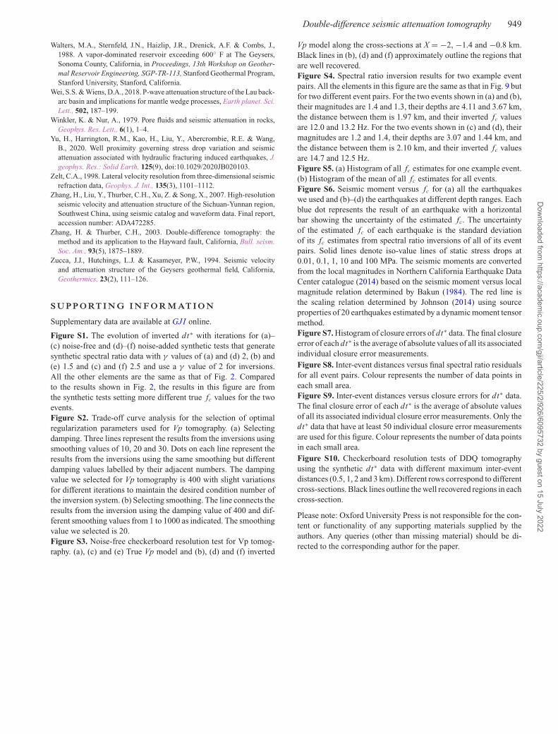
Double-difference seismic attenuation tomography 949
Walters, M.A., Sternfeld, J.N., Haizlip, J.R., Drenick, A.F. & Combs, J.,1988. A vapor-dominated reservoir exceeding 600◦ F at The Geysers,Sonoma County, California, in Proceedings, 13th Workshop on Geother-mal Reservoir Engineering, SGP-TR-113, Stanford Geothermal Program,Stanford University, Stanford, California.
Wei, S.S. & Wiens, D.A., 2018. P-wave attenuation structure of the Lau back-arc basin and implications for mantle wedge processes, Earth planet. Sci.Lett., 502, 187–199.
Winkler, K. & Nur, A., 1979. Pore fluids and seismic attenuation in rocks,Geophys. Res. Lett., 6(1), 1–4.
Yu, H., Harrington, R.M., Kao, H., Liu, Y., Abercrombie, R.E. & Wang,B., 2020. Well proximity governing stress drop variation and seismicattenuation associated with hydraulic fracturing induced earthquakes, J.geophys. Res.: Solid Earth, 125(9), doi:10.1029/2020JB020103.
Zelt, C.A., 1998. Lateral velocity resolution from three-dimensional seismicrefraction data, Geophys. J. Int., 135(3), 1101–1112.
Zhang, H., Liu, Y., Thurber, C.H., Xu, Z. & Song, X., 2007. High-resolutionseismic velocity and attenuation structure of the Sichuan-Yunnan region,Southwest China, using seismic catalog and waveform data. Final report,accession number: ADA472285.
Zhang, H. & Thurber, C.H., 2003. Double-difference tomography: themethod and its application to the Hayward fault, California, Bull. seism.Soc. Am., 93(5), 1875–1889.
Zucca, J.J., Hutchings, L.J. & Kasameyer, P.W., 1994. Seismic velocityand attenuation structure of the Geysers geothermal field, California,Geothermics, 23(2), 111–126.
S U P P O RT I N G I N F O R M AT I O N
Supplementary data are available at GJI online.
Figure S1. The evolution of inverted dt∗ with iterations for (a)–(c) noise-free and (d)–(f) noise-added synthetic tests that generatesynthetic spectral ratio data with γ values of (a) and (d) 2, (b) and(e) 1.5 and (c) and (f) 2.5 and use a γ value of 2 for inversions.All the other elements are the same as that of Fig. 2. Comparedto the results shown in Fig. 2, the results in this figure are fromthe synthetic tests setting more different true fc values for the twoevents.Figure S2. Trade-off curve analysis for the selection of optimalregularization parameters used for Vp tomography. (a) Selectingdamping. Three lines represent the results from the inversions usingsmoothing values of 10, 20 and 30. Dots on each line represent theresults from the inversions using the same smoothing but differentdamping values labelled by their adjacent numbers. The dampingvalue we selected for Vp tomography is 400 with slight variationsfor different iterations to maintain the desired condition number ofthe inversion system. (b) Selecting smoothing. The line connects theresults from the inversion using the damping value of 400 and dif-ferent smoothing values from 1 to 1000 as indicated. The smoothingvalue we selected is 20.Figure S3. Noise-free checkerboard resolution test for Vp tomog-raphy. (a), (c) and (e) True Vp model and (b), (d) and (f) inverted
Vp model along the cross-sections at X = −2, −1.4 and −0.8 km.Black lines in (b), (d) and (f) approximately outline the regions thatare well recovered.Figure S4. Spectral ratio inversion results for two example eventpairs. All the elements in this figure are the same as that in Fig. 9 butfor two different event pairs. For the two events shown in (a) and (b),their magnitudes are 1.4 and 1.3, their depths are 4.11 and 3.67 km,the distance between them is 1.97 km, and their inverted fc valuesare 12.0 and 13.2 Hz. For the two events shown in (c) and (d), theirmagnitudes are 1.2 and 1.4, their depths are 3.07 and 1.44 km, andthe distance between them is 2.10 km, and their inverted fc valuesare 14.7 and 12.5 Hz.Figure S5. (a) Histogram of all fc estimates for one example event.(b) Histogram of the mean of all fc estimates for all events.Figure S6. Seismic moment versus fc for (a) all the earthquakeswe used and (b)–(d) the earthquakes at different depth ranges. Eachblue dot represents the result of an earthquake with a horizontalbar showing the uncertainty of the estimated fc. The uncertaintyof the estimated fc of each earthquake is the standard deviationof its fc estimates from spectral ratio inversions of all of its eventpairs. Solid lines denote iso-value lines of static stress drops at0.01, 0.1, 1, 10 and 100 MPa. The seismic moments are convertedfrom the local magnitudes in Northern California Earthquake DataCenter catalogue (2014) based on the seismic moment versus localmagnitude relation determined by Bakun (1984). The red line isthe scaling relation determined by Johnson (2014) using sourceproperties of 20 earthquakes estimated by a dynamic moment tensormethod.Figure S7. Histogram of closure errors of dt∗ data. The final closureerror of each dt∗ is the average of absolute values of all its associatedindividual closure error measurements.Figure S8. Inter-event distances versus final spectral ratio residualsfor all event pairs. Colour represents the number of data points ineach small area.Figure S9. Inter-event distances versus closure errors for dt∗ data.The final closure error of each dt∗ is the average of absolute valuesof all its associated individual closure error measurements. Only thedt∗ data that have at least 50 individual closure error measurementsare used for this figure. Colour represents the number of data pointsin each small area.Figure S10. Checkerboard resolution tests of DDQ tomographyusing the synthetic dt∗ data with different maximum inter-eventdistances (0.5, 1, 2 and 3 km). Different rows correspond to differentcross-sections. Black lines outline the well recovered regions in eachcross-section.
Please note: Oxford University Press is not responsible for the con-tent or functionality of any supporting materials supplied by theauthors. Any queries (other than missing material) should be di-rected to the corresponding author for the paper.
Dow
nloaded from https://academ
ic.oup.com/gji/article/225/2/926/6095732 by guest on 15 July 2022
Related Documents