Double Averaged Turbulence Modelling in Eulerian Multi ...

Jul-04 Dresden, Germany, 2004 1 ANSYS CFX

Double Averaged Turbulence Modelling in Eulerian Multi-

Phase Flows

Alan Burns1, Thomas Frank1, Ian Hamill1 and Jun-Mei Shi2.1ANSYS CFX and 2FZ-Rossendorf


Physics Of Bubbly Flow


Multi-Phase Turbulence Phenomena

• Continuous Phase Effects On Dispersed Phase Turbulence.– Simplest model for dilute

dispersed phase Reynolds stresses:

• Turbulent Dispersion.– Migration of dispersed

phase from regions of high to low void fraction.

– Continuous phase eddies capture dispersed phase particles by action of interfacial forces.

cd uCu ′=′ jcicjdid uuCuu ′′=′′ 2

νβσ

νν tc

td =2

1

C=νβσ


Multi-Phase Turbulence Phenomena

• Dispersed Phase Effects On Continuous Phase

Turbulence.

• Turbulence Enhancement

– Due to shear production in wakes behind particles.

• Turbulence Reduction

– Due to transfer of turbulence kinetic energy to dispersed phase kinetic energy by action of interfacial forces.


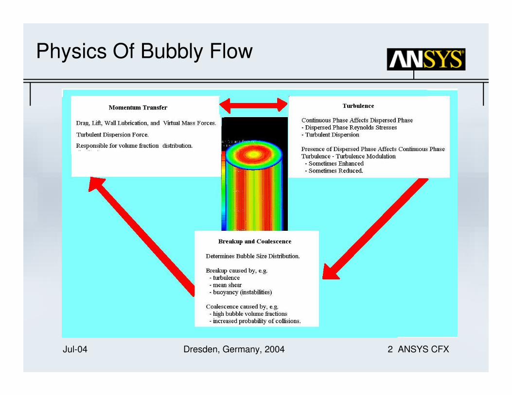
Averaging Procedures

• First Average = Phase Average

• Phase indicator function:• χα(x,t) = 1 if phase α is present, = 0, otherwise.

• Use ensemble-, time- or space-averaging to

define phase-averaged variables:

– ‘Volume Fraction’:

– Material Density

– Phase Averaged Transport Variable:

• Essentially Mass-Weighted Average

αα χ=r

ααα ρχρ r/=

ααα ρρχ /Φ=Φ


Averaging Procedures:

• Phase averaged Momentum and Continuity.

• Mαk = interfacial forces

• = Reynolds Stress like terms

• Phase induced turbulence, or full turbulence?

• Some researchers assume this represents full

turbulence, e.g. Kashiwa et al.

• We assume it represents phase-induced turbulence.

( ) ( )( )( ) kk

k

t

ikikki

i

k MBrx

PrUUr

xUr

tαααααααααααα ττρρ ++

∂

∂−=+−

∂

∂+

∂

∂

( ) ( ) 0=∂

∂+

∂

∂i

i

Urx

rt

ααααα ρρ

αααα ρτ ji

t

ik uu ′′−=


Averaging Procedures:

• Models for Phase-Induced Turbulence.

• Sato: Algebraic Eddy Viscosity:

• Kataoka and Serizawa (1989) derived exact transport

equations for kpi andε pi.

• Term identified for enhanced turbulence production:

• Exact once the terms for interfacial forces are closed.

∂

∂−

∂

∂+

∂

∂+−=

i

iij

i

j

j

ipitijpipiij

x

U

x

U

x

Uk δµδρτ

3

2,, dcpdcpit UUdrC −= ρµ µ,

( )αβαβα UUMP pik

rrr−⋅−=

,


Averaging Procedures

• Second Average = Time or Favre Average.

• Ensemble averaged phase equations are fully

space and time dependent.

• Hence, may apply a second time- average.

• Shear induced turbulence?

• Favre or Mass Weighted averaging is

favoured, as it leads to much fewer terms in

the averaged equations.


Favre Averaging

• Favre averaging of phase-averaged variables

is defined as follows:

• For constant density phases, reduces to a

volume fraction weighted average:

• Favre-averaged and time-averaged quantities

are related as follows:

αααα φ rr /~

=Φ

αααααα ρφρ rr /~

=Φ

ααααα φ rr /~

′′+Φ=Φ


Favre Averaging

• Time- and Favre- averaged velocities are related by:

• is fundamental to turbulent dispersion, as it

describes how phasic volume fractions are spread out by velocity fluctuations.

• Eddy-viscosity type turbulence models, employ eddy

diffusivity hypothesis (EDH):

• Turbulent Prandtl number is typically of order unity.

ααα uUUrrr

′′+=~

αααα ruru /rr′′=′′

α

α

ααα

σ

νrur

r

t ∇−=′′r

ααurr′′


Favre Averaging

• Time Averaged Continuity Equation

– Includes volume fraction-velocity correlation term.

– Yields additional diffusion term, if we employ the eddy diffusivity hypothesis.

• Favre Averaged Continuity Equation

– No extra terms.

– A mathematical simplification, not a physical one.

( ) ( )( ) 0=′′+∂

∂+

∂

∂ii

i

urrUx

rt

ααααααα ρρ

( ) ( ) 0~

=∂

∂+

∂

∂ααααα ρρ rU

xr

ti

i


Turbulent Dispersion Force

• Assume caused by interaction between turbulent eddies and inter-phase forces.

• Model using time average of fluctuating part of interphase momentum force.

• Restrict attention to drag force, assumed proportional to slip velocity and interfacial area density Aαβ.

• Assume Dαβ approximately constant as far as averaging procedure is concerned.

( ) ( )αβαβαβαβαβα UUADUUCMrrrrr

−=−=


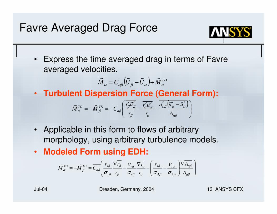
Favre Averaged Drag Force

• Express the time averaged drag in terms of Favreaveraged velocities.

• Turbulent Dispersion Force (General Form):

• Applicable in this form to flows of arbitrary morphology, using arbitrary turbulence models.

• Modeled Form using EDH:

( ) TDMUUCM ααβαβα

rr+−=

~~

( )

′−′′−

′′−

′′−=−=

αβ

αβαβ

α

αα

β

ββαββα

A

uua

r

ur

r

urCMM

TDTD

rrrrrr

∇

−−

∇−

∇=−=

αβ

αβ

α

α

β

β

α

α

α

α

β

β

β

β

αββασ

ν

σ

ν

σ

ν

σ

ν

A

A

r

r

r

rCMM

A

t

A

t

r

t

r

tTDTDrr


Polydispersed Multi-Phase Flow

• Algebraic form of area density is known:

• Hence, area density-velocity correlations may be expressed in terms of volume fraction-velocity correlations:

• General Form:

• Eddy Diffusivity Hypothesis (EDH):

β

β

αβd

rA

6=

′−

′′=−=

β

αβ

α

αααββα

r

ur

r

urCMM

TDTD

rrrr

∇−

∇=−=

α

α

β

β

α

ααββα

σ

ν

r

r

r

rCMM

r

tTDTDrr


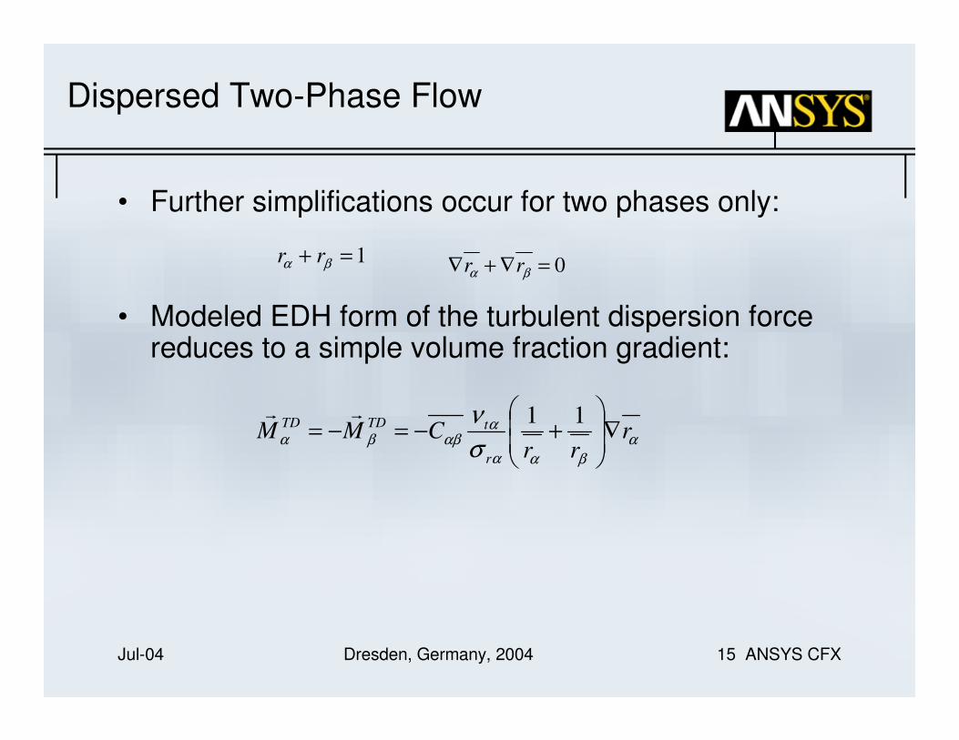
Dispersed Two-Phase Flow

• Further simplifications occur for two phases only:

• Modeled EDH form of the turbulent dispersion force reduces to a simple volume fraction gradient:

1=+ βα rr0=∇+∇ βα rr

α

βαα

ααββα

σ

νr

rrCMM

r

tTDTD ∇

+−=−=

11rr


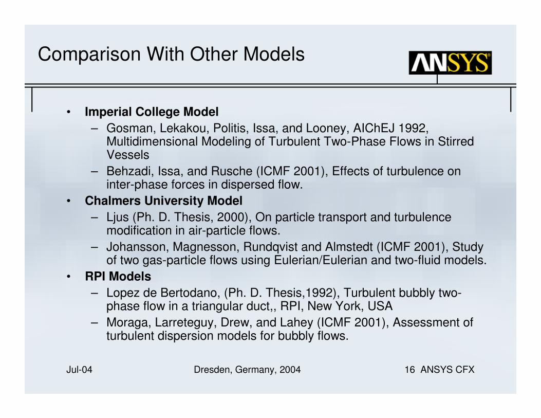
Comparison With Other Models

• Imperial College Model

– Gosman, Lekakou, Politis, Issa, and Looney, AIChEJ 1992, Multidimensional Modeling of Turbulent Two-Phase Flows in Stirred Vessels

– Behzadi, Issa, and Rusche (ICMF 2001), Effects of turbulence on inter-phase forces in dispersed flow.

• Chalmers University Model

– Ljus (Ph. D. Thesis, 2000), On particle transport and turbulence modification in air-particle flows.

– Johansson, Magnesson, Rundqvist and Almstedt (ICMF 2001), Study of two gas-particle flows using Eulerian/Eulerian and two-fluid models.

• RPI Models

– Lopez de Bertodano, (Ph. D. Thesis,1992), Turbulent bubbly two-phase flow in a triangular duct,, RPI, New York, USA

– Moraga, Larreteguy, Drew, and Lahey (ICMF 2001), Assessment of turbulent dispersion models for bubbly flows.


Imperial College Model

• Idea of modeling turbulence dispersion force by Favreaveraging drag term was first proposed by Gosman et al (1992).

• Behzadi et al (ICMF 2001) also consider lift and virtual mass forces, but found them insignificant.

• Equivalent to our model in the dilute limit.

• Hence, validation reported by Gosman et al valid for FAD model

0→βr


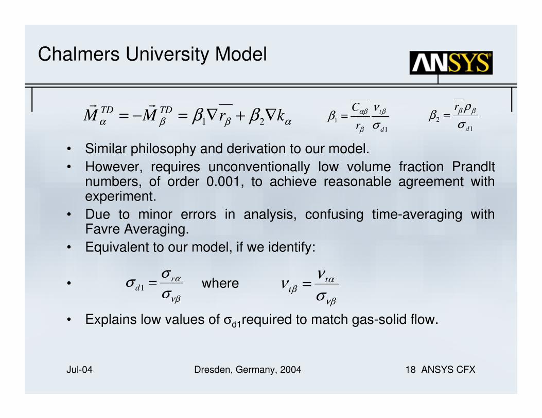
Chalmers University Model

• Similar philosophy and derivation to our model.

• However, requires unconventionally low volume fraction Prandltnumbers, of order 0.001, to achieve reasonable agreement with experiment.

• Due to minor errors in analysis, confusing time-averaging with Favre Averaging.

• Equivalent to our model, if we identify:

• where

• Explains low values of σd1required to match gas-solid flow.

αββα ββ krMM TDTD ∇+∇=−=21

rr

1

1

d

t

r

C

σ

νβ β

β

αβ=1

2

d

r

σ

ρβ ββ=

νβ

α

σ

σσ r

d =1

νβ

αβ

σ

νν t

t =


RPI Models: Lopez de Bertodano

• CTD is a non-dimensional empirical constant. – CTD = 0.1 to 0.5 gave reasonable results for medium sized

bubbles in ellipsoidal particle regime (Lopez de Bertodano et al

1994a, 1994b).

• However, flow regimes involving small bubbles or small solid particles were found to require very different values of CTD, up to 500.

• Revised by Lopez de Bertodano (1999).– Proposed that CTD be expressed as a function of turbulent

Stokes number as follows:

αααβα ρ rkCMM TD

TDTD ∇−=−=rr

)1(

14/1

StStCCTD

+= µ


RPI Models: Lopez de Bertodano

• Compare with Favre Averaged Drag (FAD) model for dispersed 2-phase flow employing EVH:

• Substitute Eddy Viscosity Formula

• Equivalent to a Lopez de Bertodano model with variable empirical constant:

• Strong function of Stokes number, as expected.

α

βαα

ααββα

σ

νr

rrCMM

r

tTDTD ∇

+−=−=

11rr

ααµα εν /2kCt =

+=

+= 1

1

41.0

11

α

β

α

µ

βαα

α

α

αβ

α

µ

σερσ r

r

St

C

rr

kCCC

rr

TD


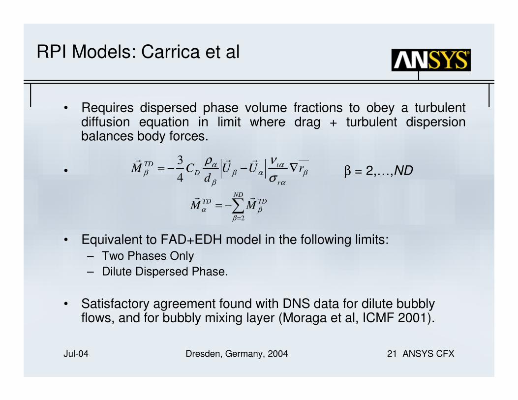
RPI Models: Carrica et al

• Requires dispersed phase volume fractions to obey a turbulent diffusion equation in limit where drag + turbulent dispersion balances body forces.

• β = 2,…,ND

• Equivalent to FAD+EDH model in the following limits:

– Two Phases Only

– Dilute Dispersed Phase.

• Satisfactory agreement found with DNS data for dilute bubbly flows, and for bubbly mixing layer (Moraga et al, ICMF 2001).

β

α

ααβ

β

αβ

σ

νρrUU

dCM

r

tD

TD ∇−−=rrr

4

3

∑=

−=ND

TDTDMM

2ββα

rr


Validation: Bubbly Flow in Vertical Pipe

• Uses Grace Drag Law

• SST turbulence model + Sato eddy viscosity.

• Compares FAD with RPI = constant

coefficient Lopez de Bertpdano model.


Liquid-Solid Flow in Mixing Vessel

• Wen Yu drag correlation for dense solids.

• SST turbulence + Sato eddy viscosity.

• Three solid lines are minimum, average and maximum values of CFD results, within region ±5mm from the data point.

• Dimension representative of size of conductivity probe.


Liquid-Solid Flow in Mixing Vessel

• Particle volume fractions underpredicted, though

correct trends are predicted.

• Similar results for 710 micron particles.


Turbulence Modulation

• Turbulence Enhancement.

• Due to turbulence production in wakes behind particles.

• Averaged out by first averaging procedure (phase averaging).

• Hence, must include in first averaged equations.


Turbulence Enhancement: Simple Models

• Sato: Treat particle-induced

and shear-induced turbulence separately.

• Algebraic Eddy Viscosity model for phase-induced turbulence:

• Modifed k-εεεε Models

• Lump particle-induced and shear-induced turbulence together.

• Add additional production terms to shear-induced k-eequations, e.g. Lee at al

dcpdcpit UUdrC −= ρµ µ,

( )2

αβαβα UUCPk

rr−=

α

α

αεα

εkPC

kP

1=

α

ααµα

ερµ

2

,,

kC sisit =

pitsitt ,, ααα µµµ +=

α

ααµα

ερµ

2k

Ct =


Turbulence Reduction

• Energy transferred from turbulent eddies to particles by acceleration of particles due to drag.

• Turbulence-drag interaction, like dispersion.

• Interaction with shear-induced turbulence, so

appears as additional source terms in 2nd averaged k-equation

ααα uMSk′⋅=rr

βββ uMSk′⋅=rr


Turbulence Reduction: Simple Model

• Chen-Wood: Consider drag only, and treat Cαβ as constant in averaging procedure:

• = velocity covariance

• Sum of sources is negative

• Hence, can only model turbulence reduction.

• Requires model for velocity covariance:

• Chen-Wood:

( ) ( ) ( )βαβαββββααβββααββ kkCuuuuCuUUCSk 2−=′′−′′=′⋅−=rrrrrrr

( ) ( ) ( )ααβαβααβααβαββαβα kkCuuuuCuUUCSk 2−=′′−′′=′⋅−=rrrrrrr

βααβ uuk ′′=rr

( ) 02

≤′−′−=+ βααββα uuCSS kk

rr

cd uCu ′=′ jcicjdic uuCuu ′′=′′


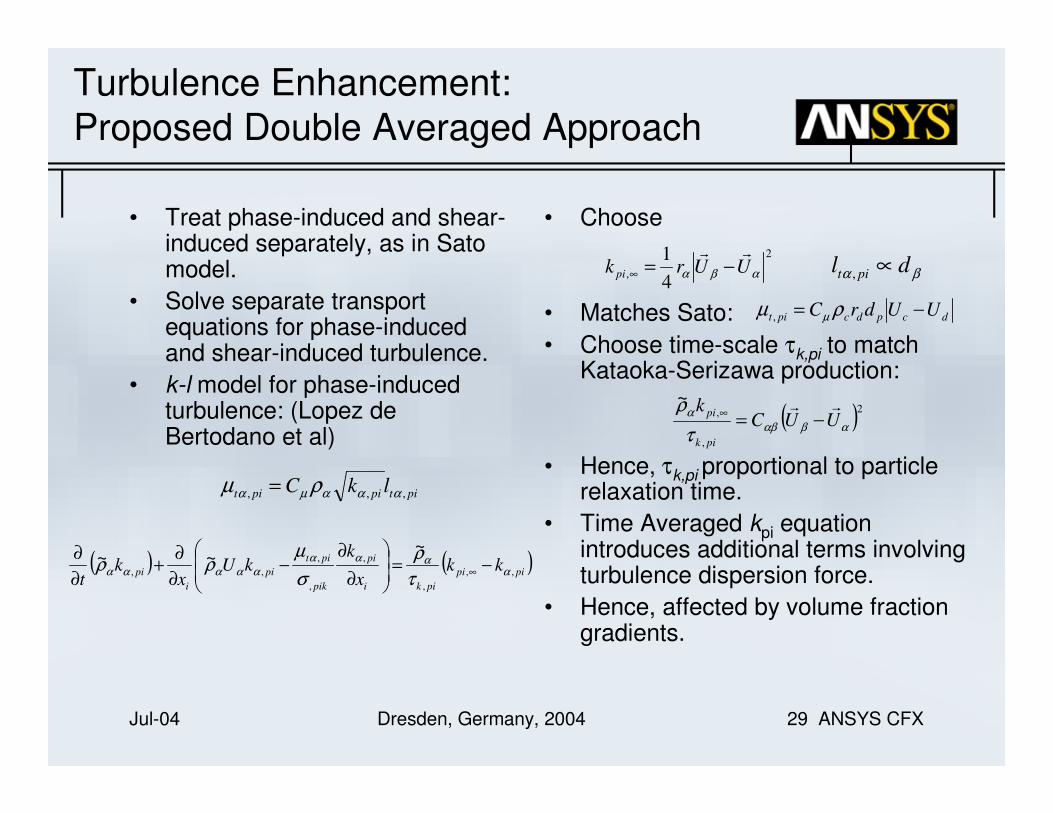
Turbulence Enhancement:

Proposed Double Averaged Approach

• Treat phase-induced and shear-induced separately, as in Sato model.

• Solve separate transport equations for phase-induced and shear-induced turbulence.

• k-l model for phase-induced turbulence: (Lopez de Bertodano et al)

• Choose

• Matches Sato:

• Choose time-scale τk,pi to match Kataoka-Serizawa production:

• Hence, τk,pi proportional to particle relaxation time.

• Time Averaged kpi equation introduces additional terms involving turbulence dispersion force.

• Hence, affected by volume fraction gradients.

( ) ( )pipi

piki

pi

pik

pit

pi

i

pi kkx

kkU

xk

t,,

,

,

,

,

,,

~~~

αααα

ααααατ

ρ

σ

µρρ −=

∂

∂−

∂

∂+

∂

∂∞

pitpipit lkC,,, αααµα ρµ =

2

,4

1αβα UUrk pi

rr−=∞ βα dl pit ∝

,

( )2

,

,

~

αβαβ

α

τ

ρUUC

k

pik

pirr

−=∞

dcpdcpit UUdrC −= ρµ µ,


Turbulence Reduction:

Proposed Double Average Approach

• As for Chen-Wood, but take area density fluctuations into account in averaging procedure.

• Hence, additional source terms in shear-induced k-equation:

• + additional terms

• Additional terms proportional to

• Hence, also affected by volume fraction gradients.

• Consider better models for velocity covariance, e.g. transport equation.

( ) ( )ααβαβαββαβαβα kkCuUUADSk 2−=′⋅−=rrr

( ) ααβαβσ

µrUUC

r

t ∇⋅−~~


Conclusions

• Double Averaging Approach yields a natural model for turbulence dispersion, with wide degree of universality.

• Implemented as default model for turbulence dispersion in CFX-5.7 (2004).

• Also produces potentially fruitful approaches to turbulence modulation.

• Topics for further investigation:– How is the model affected by taking into account non-linear

dependence of drag on slip velocity?

– How is the model affected by taking into account volume fraction dependence of the drag coefficient?

– second order closure models.

– separated flows.

Double Averaged Turbulence Modelling in Eulerian Multi ...

Documents