165 DOMESTIC SAVING AND INVESTMENT REVISED: CAN THE FELDSTEIN-HORIOKA EQUATION BE USED FOR POLICY ANALYSIS? Adolfo Sachsida Mário Jorge Cardoso de Mendonça Originally published by Ipea in February 2006 as number 1158 of the series Texto para Discussão.

Welcome message from author
This document is posted to help you gain knowledge. Please leave a comment to let me know what you think about it! Share it to your friends and learn new things together.
Transcript

165
DOMESTIC SAVING AND INVESTMENT REVISED: CAN THE FELDSTEIN-HORIOKA EQUATION BE USED FOR POLICY ANALYSIS?
Adolfo SachsidaMário Jorge Cardoso de Mendonça
Originally published by Ipea in February 2006 as number 1158 of the series Texto para Discussão.


DISCUSSION PAPER
165B r a s í l i a , J a n u a r y 2 0 1 5
Originally published by Ipea in February 2006 as number 1158 of the series Texto para Discussão.
DOMESTIC SAVING AND INVESTMENT REVISED: CAN THE FELDSTEIN-HORIOKA EQUATION BE USED FOR POLICY ANALYSIS?
Adolfo Sachsida1
Mário Jorge Cardoso de Mendonça2
1. From Universidade Católica de Brasília. E-mail: <[email protected]>.2. From Instituto de Pesquisa Econômica Aplicada. E-mail: <[email protected]>.

DISCUSSION PAPER
A publication to disseminate the findings of research
directly or indirectly conducted by the Institute for
Applied Economic Research (Ipea). Due to their
relevance, they provide information to specialists and
encourage contributions.
© Institute for Applied Economic Research – ipea 2015
Discussion paper / Institute for Applied Economic
Research.- Brasília : Rio de Janeiro : Ipea, 1990-
ISSN 1415-4765
1. Brazil. 2. Economic Aspects. 3. Social Aspects.
I. Institute for Applied Economic Research.
CDD 330.908
The authors are exclusively and entirely responsible for the
opinions expressed in this volume. These do not necessarily
reflect the views of the Institute for Applied Economic
Research or of the Secretariat of Strategic Affairs of the
Presidency of the Republic.
Reproduction of this text and the data it contains is
allowed as long as the source is cited. Reproductions for
commercial purposes are prohibited.
Federal Government of Brazil
Secretariat of Strategic Affairs of the Presidency of the Republic Minister Roberto Mangabeira Unger
A public foundation affiliated to the Secretariat of Strategic Affairs of the Presidency of the Republic, Ipea provides technical and institutional support to government actions – enabling the formulation of numerous public policies and programs for Brazilian development – and makes research and studies conducted by its staff available to society.
PresidentSergei Suarez Dillon Soares
Director of Institutional DevelopmentLuiz Cezar Loureiro de Azeredo
Director of Studies and Policies of the State,Institutions and DemocracyDaniel Ricardo de Castro Cerqueira
Director of Macroeconomic Studies and PoliciesCláudio Hamilton Matos dos Santos
Director of Regional, Urban and EnvironmentalStudies and PoliciesRogério Boueri Miranda
Director of Sectoral Studies and Policies,Innovation, Regulation and InfrastructureFernanda De Negri
Director of Social Studies and Policies, DeputyCarlos Henrique Leite Corseuil
Director of International Studies, Political and Economic RelationsRenato Coelho Baumann das Neves
Chief of StaffRuy Silva Pessoa
Chief Press and Communications OfficerJoão Cláudio Garcia Rodrigues Lima
URL: http://www.ipea.gov.brOmbudsman: http://www.ipea.gov.br/ouvidoria
DISCUSSION PAPER
A publication to disseminate the findings of research
directly or indirectly conducted by the Institute for
Applied Economic Research (Ipea). Due to their
relevance, they provide information to specialists and
encourage contributions.
© Institute for Applied Economic Research – ipea 2015
Discussion paper / Institute for Applied Economic
Research.- Brasília : Rio de Janeiro : Ipea, 1990-
ISSN 1415-4765
1. Brazil. 2. Economic Aspects. 3. Social Aspects.
I. Institute for Applied Economic Research.
CDD 330.908
The authors are exclusively and entirely responsible for the
opinions expressed in this volume. These do not necessarily
reflect the views of the Institute for Applied Economic
Research or of the Secretariat of Strategic Affairs of the
Presidency of the Republic.
Reproduction of this text and the data it contains is
allowed as long as the source is cited. Reproductions for
commercial purposes are prohibited.
JEL: F21; C22.
SUMMARY
SINOPSE
ABSTRACT
1 INTRODUCTION 1
2 THE FH REGRESSION AND THE DIFFERENT CONCEPTS OF EXOGENEITY 1
3 ARE INVESTMENT AND SAVING SERIES CO-INTEGRATED? 4
4 ESTIMATING THE FH EQUATION FOR BRAZIL 7
5 APPLYING EXOGENEITY TESTS FOR SAVING ON THE FH EQUATION 9
6 STRUCTURAL ANALYSIS FOR INVESTMENT AND SAVING 13
7 FINAL REMARKS 16
APPENDIX 17
BIBLIOGRAPHY 21


SINOPSECom base na relação entre investimento e poupança doméstica que deriva da equaçãode Feldstein-Horioka (FH), este estudo objetiva, a partir da aplicação de testes deexogeneidade, verificar de que maneira esta equação pode ser usada comoinstrumento na formulação de política econômica no Brasil. Numa etapa posterior,utilizam-se os resultados do teste de exogeneidade fraca para identificar um VARestrutural (SVAR) e obter as funções de impulso resposta (IRFs) que derivam domodelo identificado. Quanto aos resultados referentes aos testes de exogeneidadetemos que: a) a elasticidade da poupança doméstica estimada de acordo commetodologia apropriada acena na direção de uma alta mobilidade de capital para oBrasil; b) a poupança doméstica é fracamente exógena na equação FH; c) a poupançadoméstica não é fortemente exógena na equação FH, o que significa dizer que não sepode projetar o investimento com base no valor condicionado da poupançadoméstica a partir da equação FH; d) mostrou-se ainda que poupança doméstica ésuperexógena na equação FH, o que quer dizer que a crítica de Lucas não se aplica nocaso da equação FH; e e) os resultados advindos das funções de impulso-respostamostraram que o investimento é sensível a uma inovação contemporânea napoupança doméstica e que o efeito positivo permanece longo tempo. No que se refereà poupança doméstica, a resposta desta a um choque não esperado do investimentotem uma descrição um pouco mais complicada. Inicialmente a poupança domésticasofre uma ligeira queda. A seguir, este efeito se aprofunda. Numa etapa posterior oquadro se reverte, passando a poupança doméstica a sentir um efeito positivo dessechoque.
ABSTRACTBased on the relation between investment and domestic saving proposed by Feldsteinand Horioka (1980) to verify capital mobility, this study performs some exogeneitytests in order to determine the capacity of the FH equation of supporting andimplementing economic policies in Brazil. We then use the result of weak exogeneitytest to identify a structural vector autoregressive (SVAR) involving investment andsaving in order to evaluate the effect of exogenous shocks through impulse responsefunctions (IRFs) on both variables. The main findings of this paper are: a) theelasticity of domestic saving estimated using appropriate methods points out to highcapital mobility for Brazil; b) domestic saving is weakly exogenous in the FHequation; c) domestic saving is not strongly exogenous, therefore this equation shouldnot be used to make forecasts for the Brazilian economy; d) superexogeneity isaccepted for domestic saving, meaning that Lucas’ criticism does not apply; and e)the IRFs showed that investment is sensitive to contemporaneous innovation onsaving and this effect lasts for a long time. Regarding to domestic saving, the responseof this variable to a non-expected shock on investment has a more is more complicatedescription. Initially domestic saving goes down. After some lags this movementchanges and domestic saving begins to react positively to the shock.

1
1 INTRODUCTIONThe correlation between domestic saving and investment is one of the mostinteresting issues appearing in economics. Academics and policy makers frequentlyformulate questions regarding their temporal precedence and the relationshipbetween them. Feldstein and Horioka (1980) interpret this correlation as a sign ofcapital mobility. The basic idea is that in a closed economy and in a low capitalmobility scenario, internal saving finances all investment. On the other hand, in anopen economy, domestic saving would be used to obtain better returns in the world,and would not necessarily be used to finance domestic investment. Thus, a strongcorrelation between domestic saving and investment would be a sign of low capitalmobility. However, a weak correlation would indicate high capital mobility.1
This article attempts to verify the robustness of the Feldstein-Horioka (FH)equation in exogeneity tests for the Brazilian economy during the period 1947-2004.First, Section 2 presents the FH equation, introducing the different kinds ofexogeneity, and comments on the importance of these tests for economic policy. InSection 3, we perform an analysis in order to verify whether the investment andsaving series are co-integrated. Before performing the Johansen-Joselius procedure todetect co-integration, we apply the Augmented Dickey Fuller (ADF) test in order toverify whether these series follow a nonstationary process. The results of the unit rootand co-integration tests show that the investment and saving series are not stationary,and there is no long-run relationship between them. In order to verify whether therelation between investment and saving derived from FH equation is spurious or notin the sense of Granger and Newbold (1974), we estimated in Section 4 the FHequation based on three distinct methods proposed by Hamilton (1993). All theresults show that the correlation between investment and saving is not spurious. InSection 5 the exogeneity tests of weak, strong and super exogeneity are undertaken.Then, in Section 6 we use the exogeneity test results to identify a structural dynamicmodel associated with investment and saving. Using a vector autoregressive (SVAR)we evaluate the effect of the exogenous shocks by impulse response functions (IRFs)on both these variables. Final comments are reserved for Section 7.
2 THE FH REGRESSION AND THE DIFFERENT CONCEPTS OF EXOGENEITY
In a cross-section of 21 OECD countries, Feldstein and Horioka (1980) estimatedthe relation between the gross investment rate2 (INVEST) and the domestic savingrate3 (SAVING), obtaining the following equation.
SAVINGINVEST)074.0()018.0(
887.0035.0 += (1)
1. More details on the Feldstein-Horioka test can be obtained in Baxter and Crucini (1993) and Bayoumi (1990).
2. The ratio between investment and Gross Domestic Product (GDP). Investment is the gross capital formation by thepublic and private sectors, excluding inventories.
3. The ratio between gross domestic saving and GDP.
2
The authors interpreted the high value of the estimated domestic savingparameter as evidence of low capital mobility across countries. The basic idea is thatin a country with a low degree of capital mobility, such as a closed economy, alldomestic saving is used to finance domestic investment. Some authors4 do notconsider this correlation as being a sign of capital mobility. For instance, Sachsidaand Abi-Ramia (2000) state that this test does not reflect capital mobility in the realworld economy, reflecting only the variability between external and domestic saving.
In spite of the criticism, the equation proposed by FH continues to be estimatedfor several countries in an attempt to reproduce a stylized fact for the economy,5 andis also used to help formulate economic policies based on the following: a) to makeinferences regarding the elasticity of domestic saving; b) to forecast investmentconditional to domestic saving; and c) to test whether the relationship in (1) isstructurally invariant. Three types of exogeneity tests correspond to these objectives,namely, weak, strong and super exogeneity tests.
The modern treatment of this subject extends and develops the CowlesCommission approach. The classic reference here is the article by Engle, Hendry andRichard (1983), hereinafter referred to as EHR. The basic elements in the EHRtreatment are explained in terms of a bivariate data generated process (DGP). Let usconsider a simple regression model
1β εt t ty x= + (2)
where the variables ),( tt xy have a bivariate normal distribution2 2(µ ,µ ,σ ,σ ,σ )y x y x yx . The conditional distribution of ty given tx , is
2|, ~ (α β ,σ )t t ty x IN x+ . The joint distribution of ty and tx , may be written as
)()|(),( ttttt xhxygxyf = , where g involves the parameter θ , and h is the
marginal distribution of tx . The evolution of tx may be represented by a regression,
such that ttt uzx +=ϕ , which is known as the marginal equation. Based on thesetwo distributions, EHR proposed three definitions of exogeneity: weak, strong andsuper exogeneity.
A variable is said to be weakly exogenous if the inference conditional on tx does
not involve a loss of information. If the variable tx is weakly exogenous and is not
Granger caused by ty , tx is said to be strongly exogenous. Finally, if tx is weaklyexogenous, and the parameters in g remain structurally invariant to changes in the
marginal distribution of tx , then tx is said to be super exogenous.
The remainder of this section is dedicated to shedding more economic light onthe importance placed on exogeneity. With regard to weak exogeneity, this propertydoes not have a direct economic interpretation. In the absence of weak exogeneity theestimation of a single equation model would be affected by endogeneity bias,
4. Sachsida and Abi-Ramia (2000); Coakley, Kulasi and Smith (1996); Baxter and Crucini (1993) and Bayoumi (1990).
5. Hussein (1998) and Mamingi (1997).

3
meaning that the OLS estimator is biased. Thus, if saving was not weakly exogenouswith regard to the FH equation, it would not be correct to use this equation toestimate the relation between investment and domestic saving. Furthermore, itspresence is necessary for both the occurrence of super as well as strong exogeneity.Thus, the appeal of testing for weak exogeneity resides in the fact that without thisproperty the variable would have neither strong nor super exogeneity properties.
The strong exogeneity property suggests the capacity of the model to be used inforecasts. Thus, in the presence of strong exogeneity, the FH equation may be usedto make forecasts regarding future rates of investment, given certain domestic savingrates. With regard to the super exogeneity property, it allows the FH equationparameters to be used to simulate the effects of different policies. This means that, inthe presence of super exogeneity, the Lucas criticism does hold. Hence, due to thefact that the rate of domestic saving is super exogenous in relation to the rate ofinvestment, it is concluded that structural breaks in the domestic saving series did notalter the parameter of this variable in the FH equation. Therefore, policies aimed atincreasing the rate of domestic saving (or reducing it) will not be successful inchanging the parameter of this variable in the FH equation.
The consequence of super exogeneity is that the adoption of a new economicpolicy aimed at increasing (or decreasing) the share of domestic saving will not besuccessful. Thus, when the rate of domestic saving increases (decreases), the rate ofinvestment increases (decreases) at the value of the parameter β, meaning that breaksin the domestic saving series are not able to alter the FH coefficient. This way, theadoption of a new economic policy aimed at increasing the share of domestic savingthat is invested, by way of mechanisms that alter the saving series, will probably notbe successful.
A second economic interpretation of super exogeneity is that which assumes thecoefficient of saving in FH equation as expressing the degree of capital mobility,which did not change over the years, for if it had, the β parameter would not havebeen the same for the entire series. By definition, super exogeneity implies structuralinvariance. Thus, if the variable were super exogenous, this would mean that itsparameter would not change over time. So, assuming that β expresses the degree ofcapital mobility, it nevertheless remained constant over the entire period. Thus, bydefinition, if the rate of domestic saving was super exogenous, this would mean thatthe degree of capital mobility would not change over time. This result is curious, tosay the least, for it means that technological innovations were not able to influencecapital mobility.
In spite of not being very intuitive, this last result is not new in the literature, forTesar and Werner (1995), and Bekaert (1995), in financial integration studies, foundthat the volatility of financial assets is not related to any financial integrationmeasure, and does not increase as a result of financial liberalization. Thus, if weconsider volatility as a measurement of capital mobility, these studies suggest thatcapital mobility is not affected by technological innovation (which could beunderstood here as liberalization or greater integration).
4
3 ARE INVESTMENT AND SAVING SERIES CO-INTEGRATED?One important problem in applying the original EHR framework is that is commonto find in literature macroeconomic time series that are nonstationary processes withunit root [Nelson and Plosser (1982)]. Many consequences arise from this. Ingeneral, we can no longer use the standard asymptotic theory. To be more specific,two important facts may arise as a consequence of the presence of the unit root. First,the object equation (2), henceforth the conditional equation, may reflect the long runrelationship between variables. In this case, it is said that the series are co-integratedand thus the conditional equation only serves to identify what happens in the longrun. Second, when two series have unit roots and are not co-integration, theconditional equation (2) may possibly be spurious. As Montiel (1994) points out, thecorrelation between investment and saving could be caused by the state of businesscycle, i.e., both S/Y and I/Y could be functions of a third variable Y/W. In particularboth S/Y and I/Y are said to be procyclical. Yet one can imagine that governmentcould respond to current account deficits (increases I/Y in relation to S/Y) bycontracting fiscal policy to achieve an account target. Taking national (domestic)saving as the sum of private and public saving, this making national savingendogenous through its public component. In this case Hamilton (1993) definessome procedures in order to avoid spurious regression.
The unit tests can be used to check the order of integration of the variables. Theestimation is performed using annual data between 1947 and 2004. The data used toestimate the FH regression for Brazil was obtained from the IBGE (Brazilian Instituteof Geography and Statistics). Using the ADF test,6 Table 1 investigates whether theinvestment and saving series have two unit roots. For each series, the first and secondlines test the null for a single unit root. The unit root tests are done includingconstant and constant + time trends. The statistics of the time trend are reported.The lag order was chosen in order to eliminate misspecification (absence ofnormality, autocorrelation, heteroskedasticity etc). The third line presents the resultof tests for a second unit root, i.e., for a unit root test in the first difference allowingfor the alternative that the series is stationary in first differences. According to theresults of Table 1, the tests do not reject the null of nonstationarity for investmentand saving in the level, but reject the null for the series in differences.
Although the ADF test shows that there was no significant evidence against theunit root hypothesis for the series in the level, the tests are not quite confidentregarding the presence of time trend in the series. In fact, these tests do not concernthe joint hypothesis involving trend and unit root. To ascertain whether a linear timetrend is present for both series we introduced two procedures. First, following Stock
6. The Phillips-Perron and other tests like the KPSS test [Kwiatkowsky et al. (1992)] can also be used. The advantage ofthe PP test is that it is more general than the ADF test because it allows for fairly mild assumptions concerning thedistributions of the errors. The usual unit root tests are very sensible to the presence of atypical values in the sample[Frances and Haldrup (1994)]. The presence of atypical values has influence on the power of the test. In this case we canapply the KPSS test. The KPSS test inverts the null hypothesis testing the absence of unit root. The rejection of the null ofstationarity hypothesis has an even stronger significance when atypical values are present. We applied the PP and KPSStests and the results do not reject the null of nonstationarity. For economy we did not include these results in the text.They can be obtained from the authors by request.

5
and Watson (1987) each series was regressed against a constant, time and three of itslags. Second, we used the ADF test based on the OLS F statistic to test the joint nullhypothesis that β 0= and ρ 1= in the following equation
α β (ρ 1) εt t ty t y∆ = + + − ∆ + (3)
TABLE 1ADF TEST—1947-2004[H0: the series has an unit root]
Variable Equation model(1)
Lags(2)
t-ADF(3)
Critical values 1/5 %(4)
Trendb
(5)
INVEST Constant + Trend 1 –2.934 –4.128–3.490
0.0017(0.145)
INVEST Constant 4 –1.528 –3.557–2.917
-
DINVEST a
Constant 2 –5.986 –3.555–2.916
-
SAVING Constant + Trend 2 –2.177 –4.131–3.493
0.001(0.500)
SAVING Constant 4 –1.524 –3.557–2.917
-
DSAVING a
Constant 3 –6.145 –3.557–2.917
-
a The operator D means the first difference of the variable.
b t-statistic and P-value on the time trend.
Note: The series are transformed to logs.
The results of these two methodologies are shown in Table 2. The F test doesnot reject the null of β 0= and ρ 1= which means that both series follow a unit rootprocess without time trend and the test based on Stock and Watson (1987) does notfind significance for time trend.
In view of the long period of our sample one may claim that the series may besubject to structural change possibly due to the modification of the economicenvironment along this period. According to Perron (1989) the presence of one ormore structural changes could affect the validity of conclusion that the variables arenot stationary. A difficulty with the conventional unit root test, given a structuralbreak, is that the critical values are too small in absolute terms, which leads to thefrequent rejection of the hypothesis of the unit roots.7 Although, as one can see, sinceour unit root test does not reject the hypothesis of nonstationarity, there is no needto apply a specified method to check for a unit root in presence of structural change.In the following section we will study structural change using parameter stability testsfor the estimated VAR which is requested before implementing co-integrationanalysis.
7. Zivot and Andrews (1992) developed a rigorous methodology to address the problem of structural change based onan earlier study by Perron (1989).
6
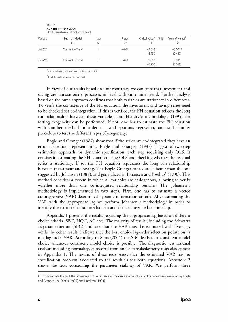
TABLE 2ADF TEST—1947-2004[H0: the series has an unit root and no trend]
Variable Equation Model(1)
Lags(2)
F-stat(3)
Critical valuesa 1/5 %
(4)Trend (P-value) b
(5)
INVEST Constant + Trend 1 –4.64 –9.312–6.730
–0.0017(0.447)
SAVING Constant + Trend 2 –4.61 –9.312–6.730
0.001(0.556)
a Critical values for ADF test based on the OLS F statistic.
b t-statistic and P-value on the time trend.
In view of our results based on unit root tests, we can state that investment andsaving are nonstationary processes in level without a time trend. Further analysisbased on the same approach confirms that both variables are stationary in differences.To verify the consistence of the FH equation, the investment and saving series needto be checked for co-integration. If this is verified, the FH equation reflects the longrun relationship between these variables, and Hendry`s methodology (1995) fortesting exogeneity can be performed. If not, one has to estimate the FH equationwith another method in order to avoid spurious regression, and still anotherprocedure to test the different types of exogeneity.
Engle and Granger (1987) show that if the series are co-integrated they have anerror correction representation. Engle and Granger (1987) suggest a two-stepestimation approach for dynamic specification, each step requiring only OLS. Itconsists in estimating the FH equation using OLS and checking whether the residualseries is stationary. If so, the FH equation represents the long run relationshipbetween investment and saving. The Engle-Granger procedure is better than the onesuggested by Johansen (1988), and generalized in Johansen and Joselius8 (1990). Thismethod considers a system in which all variables are endogenous, allowing to verifywhether more than one co-integrated relationship remains. The Johansen`smethodology is implemented in two steps. First, one has to estimate a vectorautoregressive (VAR) determined by some information criteria. After estimating theVAR with the appropriate lag we perform Johansen`s methodology in order toidentify the error correction mechanism and the co-integrated relationship.
Appendix 1 presents the results regarding the appropriate lag based on differentchoice criteria (SBC, HQC, AC etc). The majority of results, including the SchwartzBayesian criterion (SBC), indicate that the VAR must be estimated with five lags,while the other results indicate that the best choice lag-order selection points out aone lag-order VAR. According to Sims (2005) the SBC leads to a consistent modelchoice whenever consistent model choice is possible. The diagnostic test residualanalysis including normality, autocorrelation and heteroskedasticity tests also appearin Appendix 1. The results of these tests stress that the estimated VAR has nospecification problem associated to the residuals for both equations. Appendix 2shows the tests concerning the parameter stability of VAR. We perform three
8. For more details about the advantages of Johansen and Joselius`s methodology to the procedure developed by Engleand Granger, see Enders (1995) and Hamilton (1993).

7
different tests for each VAR equation; the recursive residuals, the CUNSUM ofsquares test, and the N-step forecast test. Neither shows a serious stability problem.In practice, this means that there is no need to use in estimations some specificprocedure that considers structural change. Finally, the results of co-integration testsbased on the Johansen-Joselius procedure are listed in Table 3.
TABLE 3JOHANSEN-JUSELIUS COINTEGRATION RANK TESTS
Lag
Order
Ho:
rank
ML
Statistic
Trace
Statistic
ML
1%
ML
5%
Trace
1%
Trace
5%
5 p <= 0
p <= 1
15.47
3.17
18.64
3.17
18.63
6.55
14.07
3.76
20.04
6.64
15.41
3.76
Notes: ML = Max-Lambda. Critical values are based on Osterwald-Lenum tabulated values.
Neither the ML test nor the Trace test shows any evidence of co-integration.This means that one cannot observe any long-run relationship between investmentand saving. Because both investment and saving are nonstationary series with unitroot, the standard asymptotic theory does not apply. In this case, in accordance toGranger and Newbold (1974), the FH equation may suggest the absence of anyconsistent relationship between these variables. Thus, one cannot pose anythingrelated to the FH equation without further investigation. Furthermore, one cannotperform any exogeneity test without first resolving this question.
4 ESTIMATING THE FH EQUATION FOR BRAZILAs Hamilton (1993) points out there are three ways in which the problems associatedto spurious regression can be avoided. The first is to include lagged values of both thedependent and independent variables in the regression. According to Hamilton(1993), it can be shown that OLS regression of the equation (3) yields consistentestimation.9 In this study we denote equation (3) by the augmented FH (AFH)equation.
1 21 1
α β φ ( ) φ ( ) εT T
t t i t i ti i
INVEST SAVING i SAVING i INVEST− −= =
= + + + +∑ ∑ (3)
The second approach differentiates the data before estimating the relation, as in:
α βt t tINVEST SAVING u∆ = + ∆ + (4)
Clearly, since the regressors and error term are I(0) in (4), under the nullhypothesis the parameters of the regression based on (4) converge to Gaussianvariables. Any t or F test based on regression (4) has the usual limiting Gaussian or
9. However a F-test of the joint null hypothesis that β , s̀1φ and s̀2φ are zero has a
nonstandard distribution.

8
Chi2 distribution. A third approach is to estimate FH equation with the Cochrane-Orcutt adjustment for first-order serial autocorrelation of the residuals. Blough(1992) showed that the Cochrane-Orcutt GLS regression is thus equivalent to thedifferentiated equation (3). It is important to pose that, according to Hamilton(1993), if the data are really stationary, then differencing the data can result in amisspecified regression. Table 4 shows the results of the FH equation estimated witheach one of these methodologies, in columns (2)-(4).
The results appearing in Table 4 show that although investment and saving arenot co-integrated variables, the FH equation is not spurious. The elasticity of savingin the FH regression is significant for the method applied. The results appearing incolumns (2)-(4) converge their results. The saving elasticity coefficients estimatedwith the three methods are very similar. Table 4 also shows in column (1) the resultsrelated to the FH equation estimated without correction.
Comparing the elasticity of saving estimated without correction to the oneestimated using appropriate methods, one can see that if we do not consider the biasthe idea regarding the relationship between investment and saving would becompletely wrong. If one interprets the saving coefficient related to capital mobility,the biased elasticity is associated to low mobility of capital and the elasticity estimatedby the appropriate estimators points to high capital mobility. This indicates thepossibility of using this equation in formulating economic policy. It is now necessaryto perform the exogeneity test. This will be done in the next section.
TABLE 4ESTIMATED REGRESSIONS FOR THE FH EQUATION
Method =
Estimator =
Dep. Variable =
OLS
INVEST
(1)
Method 1
OLS
INVEST a
(2)
Method 2
OLS
DINVEST(3)
Method 3
C.-Orcutt GLS
INVEST(4)
Ind. Variables Coeff. P-value Coeff. P-value Coeff. P-value Coeff. P-value
Constant
SAVINGDSAVINGINVEST_1INVEST_2SAVING_1SAVING_2AR
L1
L2
L3
Normalityb
0.654
0.784
-
-
-
-
-
-
-
-
-
0.026
(0.020)
(0.000)
-
-
-
-
-
-
-
-
-
0.986
0.527
0.363
-
0.872
–0.321
–0.123
–0.022
-
-
-
-
2.02
(0.046)
(0.003)
(0.000)
(0.095)
0.402
0.866
-
-
-
-
0.3635
0.008
-
0.352
-
-
-
-
-
-
-
-
0.346
(0.000)
-
(0.000)
-
-
-
-
-
-
-
-
0.840
0.058
0.371
0.352
-
-
-
-
-
0.879
–0.153
0.111
-
(0.000)
(0.000)
-
-
-
-
-
-
(0.000)
(0.463)
(0.419)
-
Notes: D = first difference, _1: first lag of the variable, AR = autoregressive error term regression, L1 = first lag of the error term. P-value in parenthesis.INVEST and SAVING in log.a The OLS regression was estimated using five lags. For economy we present the results up to lag two.
b The Jarque-Bera statistic has a distribution with two degrees of freedom under the null hypothesis of normally distributed errors.

9
5 APPLYING EXOGENEITY TESTS FOR SAVING ON THE FH EQUATION
In the last section, based on a rigorous methodology regarding the nonstationaryprocess for investment and saving for the Brazilian economy, we reached thefollowing conclusions: a) the investment and domestic saving series are I(1); b) theyare not co-integrated; and c) the FH equation is not spurious. Hendry (1995)developed an interesting analysis to perform exogeneity considering the existence of aunit root and cointegration. In view of (c), we cannot apply the Hendry analysisdirectly. In order to perform the exogeneity test in the present context, we use thefollowing system of equations involving the variables SAVING and INVEST asfollows:
α β ,tINVEST SAVING u∆ = + ∆ + (5.1)
1 2 11
λ ( ) λ ( ) ε ,T T
t t i t i ti i
SAVING i INVEST i SAVING− −=
∆ = ∆ + ∆ +∑ ∑ (5.2)
1 2 21 1
( ) ( ) ε ,T T
t t i t i ti i
INVEST i SAVING i INVEST− −= =
∆ = φ ∆ + φ ∆ +∑ ∑ (5.3)
Based on 5.1, 5.2 and5.3, the following proposition can be placed:
a) equation 5.1 represents the correct form of estimating the FH equationaccording to the methods of differences proposed in Section 4;
b) equation 5.2 and 5.3 are the marginal processes;
c) 1λ ( ) 0i ≠ and 1( ) 0iφ = determine the failures of the Granger-causality ofSAVING on INVEST; and
d) The condition that 1 2σ(ε ,ε ) 0t t ≠ determines the presence ofcontemporaneity, where 1 2σ(ε ,ε )t t is the correlation between 1ε t and 2ε t .
In view of the commentaries posed in last section, the conditional equation mustbe placed on differences in order to be correctly specified. Due to the presence of unitroot, the Granger causality test on a VAR in levels is biased10 which means that wehave to apply this test in VAR on differences represented by equations 5.2 and 5.3.Lastly, contemporaneity will continue to be tested as it appears in item (c) using theresiduals of a VAR on differences.
10 As Sims, Stock and Watson point out the asymptotic distribution of causality tests are sensitive to unit root and timetrends in the series. The analysis of causality between investment and savings will be performed in Section 5.2.

10
5.1 WEAK EXOGENEITY AND CONTEMPORANEITY
In models of only one equation, if the variables on the right side are not exogenous,then the coefficient estimated is biased. Thus, in a model of one equation, it isnecessary to warrant that the right-side variables are exogenous. The statistical testthat verifies this condition is the test of weak exogeneity. In order to test weakexogeneity for the variable saving in conditional equation (5.1) we use the LM testdeveloped by Engle (1984) and the Durbin-Wu-Hauman test [Durbin (1953), Wu(1973) and Hausman (1978)]. In order to perform the Engle test the error ofconditional equation (5.1) is included in the equation (5.2). If the error ofconditional equation is not statistically significant in this marginal process for saving,then this means that domestic saving is weakly exogenous in the FH equation. Table5 shows the results of this test. As one can see, the coefficient of the error of theconditional equation in the marginal is not significant.
The Durbin-Wu-Hauman test is done using the estimated results of equation(5.1) obtained by ordinary least squares (OLS) and an instrumental variable (IV).The null hypothesis states that an (OLS) estimator of the same equation would yieldconsistent estimates: that is, any endogeneity among the regressors would not havedeleterious effects on OLS estimates.11 A rejection of the null indicates thatendogenous regressors' effects on the estimates are meaningful, and IV techniques arerequired. We also evaluated another test statistic to check for endogeneity in the Wu-Hausman [Wu (1973), Hausman (1978)]12 In this case, a rejection of the nullindicates that the instrumental variable estimator should be employed. The resultsappear on the right side of Table 5. Based on the results of these two tests weconclude for the weak exogeneity of domestic saving in the FH equation.
TABLE 5WEAK EXOGENEITY TESTS
1 The LM test
Statistical significance of error of conditional equation (5.1)
in the marginal equation (5.2):
Coeff (P-value) = -0.154 (0.443)
2 The Durbin-Wu-Hauman test.
H0: Regressor is exogenous
Chi-sq[1] (P-value) = 0.0137 (0.9070)
3 The Wu-Hauman test
H0: Regressor is exogenous
F[1,52] (P-value) = 0.0129 (0.9099)
Note: P-value in parenthesis. We use the lags of the differences of variables SAVING and INVEST as instruments.
The contemporaneity test proposed by Engle (1984) consists of verifying thecorrelation between the errors of equation (5.2) with the errors of the conditionalequation (5.1). This test is based on the coefficient estimated by the OLS regression
11. Under the null, it is Chi-squared distributed with m degrees of freedom, where m is the number of regressorsspecified as endogenous in the original IV regression.
12. It can be showed that this test could be calculated straightforwardly through the use of auxiliary regressions. The teststatistic, under the null, is distributed F(m,N-k), where m is the number of regressors specified as endogenous in theoriginal instrumental variable regression.
11
between the residuals of equation (5.1) and (5.2). Under the null there is nocontemporaneity. We performed the regression and the t test showed that we couldnot reject the null hypothesis that the correlation is 0. Then, we verified that there isno contemporaneity according to this test.
5.2 STRONG EXOGENEITY
If domestic saving is strongly exogenous in the FH equation, this means that thisequation can be used to make forecasts. But if the independent variable is notstrongly exogenous, then the FH equation cannot be used to make forecasts. Thestrong exogeneity of SAVING property in the FH equation is comprised of tworequisites: a) SAVING is weak exogeneity; and b) INVEST does not cause SAVINGin the Granger sense. Requisite a was demonstrated in Subsection 5.1. Thus, fordomestic saving to be strongly exogenous and for the FH equation to be used tomake forecasts, we only need to demonstrate requisite b.
It may be useful to point out that the Granger causality test is not a test that isused to verify causality with respect to established temporal precedence. In theGranger causality test, four alternatives are possible: 1) SAVING Granger causesINVEST, but the contrary is not true; 2) INVEST Granger causes SAVING, but thecontrary is not true; 3) SAVING Granger causes INVEST and the contrary is true;and 4) SAVING not Granger causes INVEST and INVEST not Granger causesSAVING. To accept the strong exogeneity of SAVING it is necessary to obtain thealternative 1.
The operational form of the Granger causality test related to the integratedvariables I(1) is to test the hypothesis in item (b) of Section 3. In view of the presenceof unit root the Granger test on a VAR in level is based [Hamilton (1993)]. Then, inorder to apply the Granger test in this context of both the variable being I(1) and notco-integrated we have to use the first to estimate a VAR on difference and use theGranger causality methodology. The majority of information criteria indicate fourlags for the VAR on difference. The Granger causality test is shown in Table 6. Theresults show that investment Granger causes domestic saving, but that the contrary isnot true (alternative 2). Thus, the FH equation cannot be used to make forecastsregarding the Brazilian economy. In the next section, the robustness of the FHequation with regard to policy changes will be verified.
TABLE 6GRANGER CAUSALITY TEST
Equation Excluded Chi2 Lags Prob > chi2
DSAVING DINVEST 20.333 4 0.000
DSAVING All 20.333 4 0.000
DINVEST DSAVING 5.630 4 0.228
DINVEST All 5.630 4 0.228

12
5.3 SUPEREXOGENEITY
The superexogeneity test allows an econometric model to escape from the Lucascriticism.13 Lucas (1976) argued that, under a rational expectation hypothesis,econometric models could not be used to formulate economic policy because, whenthe policy maker changes the policy, the agents change their behavior. Consequently,the parameter found before the political change would not be the same after thechange. However, in an article on the consumption function in the United Kingdom,Davidson et al. (1978) presented conditions under which Lucas’ criticism does notapply. The variables that satisfied these conditions were labeled super exogenous.Whenever a variable is super exogenous, policy makers can use it to formulateeconomic policies. In this section, we propose two tests in order to verifysuperexogeneity. First, we employed the testing framework suggested by Engle andHendry (1993). To implement this methodology, a marginal model for saving mustbe proposed. We implement the Engle and Hendry (EH) test using the equation (6)as the marginal stochastic process for domestic saving.
1
α
p
t j t j tj
saving savingϕ ν−=
= + +∑ (6)
The idea of the EH test is to include the squared residuals of the marginalequation (6) and its lags in the conditional equation represented by the FH or AFHequation. If the squared residuals of the marginal equation and its lags were notstatistically significant in the conditional equation, then this would indicate theacceptance of superexogeneity. Table 7 displays the results of the EH test applied forboth the FH and AFH equations. The results show that one cannot find evidence toreject the hypothesis that domestic saving is superexogenous in the FH or AFHequations.
For the second test of superexogeneity we will apply the approach proposed byCharemza-Király [CK test (1990)]. The idea of this test is to estimate a regressionwhere the forecast error of the conditional equation is the dependent variable. Thefirst difference of domestic saving and its lags are the independent variables. Toaccept superexogeneity, the independent variables should not be statisticallysignificant. This test has an advantage in relation to other superexogeneity tests, for itdoes not need a marginal equation. Table 7 shows the results of this test. As one cansee, the difference of domestic saving and its lags are not statistically significant in theregression where the forecast error of the conditional equation is the dependentvariable. Thus, the CK test accepts that saving is superexogenous in the FH equation.In summary, both tests we performed in this section did not reject superexogeneityhypothesis.
13. A discussion of the empirical relevance of the Lucas criticism was put forth by Ericson and Irons (1995).

13
TABLE 7SUPEREXOGENEITY TESTS
1 Engle and Hendry (EH) test
Statistical significance of error and its lags of the marginal
process for saving (7) in the conditional equation:
FH equation (4)
F test (Prob > F) = –1.28 (0.291)
AFH equation (3):
F test (Prob > F) = 1.27 (0.299)
2 Charemza-Király test
Statistical significance of the first difference of domestic saving and
its lags error in forecast error (FE) of the conditional equation
FE of FH equation (4)
F test (Prob > F) = –0.44 (0.778)
FE of AFH equation (4):
F test (Prob > F) = 0.02 (0.998)
Note: Instruments: lags of investment and saving. The F-test of the first stage rejects the null hypothesis that the instruments are weak.
6 STRUCTURAL ANALYSIS FOR INVESTMENT AND SAVINGIn order to explore the usefulness of the exogeneity tests performed in this study, inthis section we consider a structural model consisting of investment and domesticsaving. The question posed is the extent to which the investment affects saving andvice-versa. In this context we have two hypothesis of interest. First, can domesticsaving be considered an exogenous variable in for the purpose of investmentmodeling. In other words, the OLS regression yields consistent estimation of thestructural parameters. The second hypothesis is a considerably stronger conjectureabout the lack of feedback from investment to domestic saving. We resume these twoconjectures in the following way. Does domestic saving exert any influence, eitherdirectly (contemporaneously) or indirectly (with a lag) on investment? Unfortunatelyin the absence of prior restriction derived from theory, neither of these twohypotheseses can be tested [Jacobs, Leamer and Ward (1979)].
To make these points more clear we consider the following structural modelinvolving invest and saving,14
1 11 1 12 1 1α β β β εt t t t tinvest saving invest saving− −= + + + + (7)
2 21 1 22 1 2α δ β β εt t t t tsaving invest invest saving− −= + + + + (8)
where 1ε t and 2ε t are independent, serially uncorrelated random variables with zeromean and constant variance. The reduced form of this structural system is given by
[ ] 1
21t t t
uinvest invest
usaving saving −
= Π +
14. For simplification we work with just one lag.

14
where Π is the matrix
11 21 12 221
11 21 12 22
β ββ β ββ(1 βγ)
γβ β γβ β
− + + Π = − + + (9)
and
1 11
2 2
ε1 β(1 βγ)
εγ 1t t
u
u− = −
(10)
According to [Jacobs, Leamer and Ward (1979)] the assumption of exogeneity isunder-identifying or just-identifying and hence is not testable, but a set of over-identifying restriction on the parameter space can be tested [Cooley and LeRoy(1985)]. Therefore if the hypothesis of exogeneity is included with sufficient numberof other restriction (sufficient to over-identifying the model), a joint test ofexogeneity can be conducted [Wu (1973) and Hausman (1978)]. In section 5.1 theLM test and the Durbin-Wu-Hauman test do not reject the hypothesis that domesticsaving is exogenous in the FH equation. We observe the same diagnostic when weperform these tests for the equation (7). Based on this point we propose to include inthe structural dynamic generating process for investment and saving expressed by (6)-(7) the constraint that β 0= . Taking this point into consideration, the system (7)-(8)can be rewritten as
1 11 1 12 1 1α β β β εt t t t tinvest saving invest saving− −= + + + + (7)
2 21 1 22 1 2α β β εt t t tsaving invest saving− −= + + + (8’)
It is important to note that Granger causality does not guarantee neither of thehypothesis posed in the beginning of this section. To see this, in order thatinvestment does not cause saving in Granger sense we must have 11 12γβ β 0+ = . But,in order the disturbance in the equation (7) is never transmitted to (8) the followingjoint restriction that 21β β 0= = must be satisfied.
The dynamic structural generating process expressed by (7)-(8’) can be used tohelp us evaluate economic performance. Our objective is to verify the effect of theexogenous shock of saving on investment, and vice-versa, using the impulse responsefunctions (IRFs). The advantage of this instrument is that it is immune to Lucas’critique because it considers only the effects of new non-expected information. Forinstance a shock to saving or investment in a country could replicate that of shocks toworld economy related to these variables.
The implementation of the dynamic structural analysis may initially be done bynoting that the stochastic process modeled by (7)-(8’) may be viewed as structuralvector autoregressive (SVAR) with the restriction that the investment does not affect

15
saving contemporaneously. This restriction derives from the weak exogeneity test. Itmust be said that weak exogeneity for saving derived from section 5.1 does notguarantee that this identification is the only one [Cooley and LeRoy (1985)], [Jacobs,Leamer and Ward (1979)]. But this one is consistent to the theory and it also appearsmore plausible for us taking the tests of weak and strong exogeneity in consideration.Taking ),( savinginvestyt = , the system (7)-(8) can be cast in the following way,
0 1 1 1... µt t t p tA y a A y A y− −= + + + + (9)
whereµ ~ (0, )t N I . The restrictions appearing in (7)-(8) imply that the element (2,1)of matrix 0A is are zero.15 Unfortunately the SVAR cannot be estimated directly.This can be done using a reduced form VAR such that,
1 1 ... ωt t p t p ty b B y B y− −= + + + + (10)
with:
ω ~ (0, )t N Σ and ''`(ω ω ) 0,t sE t s= ∀ ≠
The relation between models (8) and (9) is based on the following identitiesaAb 1
0−= , ii AAB 1
0−= and 1
0ω µt tA−= . We can retrieve the SVAR from the reduced
form VAR using the following relation: 1 , 1 ' 1 1 '0 0 0 0(ε ε )( ) ( )t tA E A A A− − − −Σ = = . Without
additional restrictions, we cannot recover the structural form because Σ does nothave enough estimated coefficients to recover an unrestricted 0A matrix.16 We callattention to an important point related to economic analysis which is that thereduced form VAR does not allow for the identification of the effects of exogenousindependent shocks to the variables because the VAR reduced form residuals arecontemporaneously correlated (the Σ matrix is not diagonal).17
The usual procedure used to estimate VAR is a special case of seeminglyunrelated regression (SURE) in which the explanatory variables are identical in allequations. In general SURE, the error covariance matrix is not diagonal, thus theestimation must be done using GLS (generalized least square) methodology.18 In ourcase 0A is just identified and one can retrieve structural parameters of 0A from Σdirectly because the number of equations and variables is the same. The case we
15. We also impose for normalization that the elements of the principal diagonal of 0A are equal to 1.
16. In our case, matrix 0A is just identified because we imposed the constraint that the element (2,1) of 0A is zero.This means that 0A is upper superior. Because the VAR is composed by only two variables, the identification can bedone necessarily in this triangular faction.
17. That is, the reduced form residuals (νt) can be interpreted as the result of linear combinations of exogenous shocksthat are not contemporaneously (in the same instant of time) correlated. It is not possible to distinguish which exogenousshocks affect the residual of each reduced form equation.
18. This point implies that in VAR we have got a striking result in which (GLS) and (LS) least square generate the sameresult.
16
examine in this study links just-identified SVAR to constraint in lag, and it is notdifficult to solve. This can be done estimating the reduced form VAR,19 whichenables us to retrieve the matrix 0A using the methodology described below. Becausewe impose the constraint that elements of the principal diagonal of 0A are equal toone, only the element (1,2) of this matrix has to be estimate.
Appendix C displays the structural IRFs. According to the results one canobserve that a non-expected temporary shock in saving implies a positive effect oninvestment and the effect of this shock lasts for a long time. Concerning to domesticsaving, the response of this variable to a non-expected shock on investment has amore complicated description. At the beginning, the domestic saving reactsnegatively and this effect remains for about six years. After it, the effect of theinnovation on investment changes and domestic saving begins to react positively tothe shock.
7 FINAL REMARKSIn this section we will interpret the results obtained in this study. First, we analysethe results of the exogeneity tests derived from the FH equation in order todetermine how this instrument can be used in economic policy analyses. Accordingto Favero (2001), these three concepts of exogeneity are useful in defining the validityof the reduction from the data-congruent reduced form and the adopted structuralequation. The exogeneity tests showed evidence that saving is weak and superexogenous but not strong exogenous in the FH equation. Concerning the weakexogeneity, this means that if the objective is to infer the parameter associate tosaving, β , the reduced form expressed by the FH or the AFH equation can in fact beused to obtain the parameter of interest. On the other hand, if the objective of theanalysis is dynamic simulation, then one cannot use the FH to make forecasts inorder to predict future behavior of investment conditioned by the anticipated valueof saving. As Favero (2001) points out, it is possible to admit a situation as the onewe observed, where saving do not cause investment in the Granger sense, but isweakly exogenous because Granger-causality is independent from the choice of theparameters of interest. The superexogeneity test showed that the FH equation it isnot subject to Lucas’ criticism. Thus, one can use the FH equation in econometricpolicy evaluation. Second, comparing the elasticity of saving estimated usingappropriate methods, one can see that this coefficient points out to high capitalmobility.
Finally, the IRFs derived from the SVAR showed that investment is sensitive tocontemporaneous innovation on saving and the major positive impact lasts for someyears. The effect of an innovation of investment on saving is more complicated.Initially domestic saving goes down. After some lags this movement changes anddomestic saving begins to react positively to the shock.
19. The Bayesian Schartz criterium indicates lag length equal to five.

17
APPENDIX A
TABLE A1INFORMATION CRITERION
Inf. Crit. = LR
5
FPE
5
AIC
5
HQIC
1
SBIC
1
Notes: LR = , FPE = Forecast Predictor Error, AIC = Akaike Information Criterion HQIC = Hanna-Quin Criterion, SBIC = Scharwz Criterion.
TABLE A2RESIDUAL DIAGNOSTIC FOR VAR
AR 1-2
F-statistics
Xi^2a
F-statistics
Portmanteau ARCHb
F-statistic
Normalityc
Chi^2
INVEST 0.507
(0.605)
1.8209
(0.108)
0.258
_
2.183
(0.147)
2.17
(0.34)
SAVING 0.520
(0.598)
1.802
(0.119)
0.281
_
2.083
(0.156)
2.61
(0.27)
SYSTEM 1.426
(0.199)
3.29
(0.50)
7.860
_
_
_
2.827
(0.30)
Notes: AR1-2 Lagrange Multiplier test for order 1-2 autocorrelation, H0=white noise.a Homoscedasticity vs residual heteroscedasticity.
b Constant variance vs residual ARCH.
c The Jarque-Bera statistic has a distribution with two degrees of freedom under the null hypothesis of normally distributed errors. The H0 hypothesis is
normality.
APPENDIX B
STABILITY TESTS FOR VAR
GRAPH 1RECURSIVE RESIDUALS: INVESTMENT
–0.4
–0.3
–0.2
–0.1
0
0.1
0.2
0.3
0.4
65 70 75 80 85 90 95 00
R ec urs ive R es iduals ± 2 S .E .

18
GRAPH 2RECURSIVE RESIDUALS: SAVING
-0.6
-0.4
-0.2
0
0.2
0.4
0.6
65 70 75 80 85 90 95 00
Recursive Residuals ± 2 S.E.
GRAPH 3CUSUM OF SQUARES TEST: INVESTMENT
- 0 .4
0 .0
0 .4
0 .8
1 .2
1 .6
6 5 7 0 7 5 8 0 8 5 9 0 9 5 0 0
C U S U M o f S q u a r e s 5 % S ig n if ic a n c e
GRAPH 4CUSUM OF SQUARES TEST: SAVING
-0 .4
0 .0
0 .4
0 .8
1 .2
1 .6
6 5 7 0 7 5 8 0 8 5 9 0 9 5 0 0
C U S U M o f S q u a re s 5 % S ig n if ic a n c e

19
GRAPH 5N STEP FORECAST TEST: INVESTMENT
0.00
0.05
0.10
0.15–0.4
–0.2
0
0.2
0.4
65 70 75 80 85 90 95 00
N -S tep Probability R ecurs ive R esiduals
GRAPH 6N STEP FORECAST TEST: SAVING
0.00
0.05
0.10
0.15 –0.8
–0.4
0
0.4
0.8
65 70 75 80 85 90 95 00
N -S tep P robability R ec urs ive R es iduals

20
APPENDIX C
IRFs-STRUCTURAL VAR
-.04
.00
.04
.08
1 2 3 4 5 6 7 8 9 10
Response of INVEST to INVEST
-.04
.00
.04
.08
1 2 3 4 5 6 7 8 9 10
Response of INVEST to SAVING
-.12
-.08
-.04
.00
.04
.08
.12
1 2 3 4 5 6 7 8 9 10
Response of SAVING to INVEST
-.12
-.08
-.04
.00
.04
.08
.12
1 2 3 4 5 6 7 8 9 10
Response of SAVING to SAVING
Response to Structural One S.D. Innovations ± 2 S.E.
21
BIBLIOGRAPHYBAXTER, M., CRUCINI, M. Explaining saving-investment correlations. The American
Economic Review, v. 83, n. 3, p. 416-436, 1993.
BAYOUMI, T. Saving-investment correlations: immobile capital, government policy orendogenous behavior. IMF Staff Papers, v. 37, p. 360-387, 1990.
BAYOUMI, T., MacDONALD, R. Consumption, income, and international capital marketintegration. Staff Papers, v. 42, n. 3, p. 552-576, Sep. 1995.
BEKAERT, G. Market integration and investment barriers in emerging equity markets.World Bank Economic Review, v. 9, n. 1, p. 75-107, 1995.
BLOUGH, S. Spurious regression with AR(1) correction and unit root pretest. John HopkinsUniversity, 1992 (Mimeo).
CHAREMZA, W. W., KIRÁLY, J. Plans and exogeneity: the genetic-teoleological disputerevised. Oxford Economic Papers, v. 42, p. 562-573, 1990.
COAKLEY, J., KULASI, F., SMITH, R. Current account solvency and the Feldstein-Horioka puzzle. Economic Journal, v. 106, n. 436, p. 620-627, 1996.
COOLEY, F. T., LeROY, S. F. Atheoretical macroeconometrics: a critique. Journal ofMonetary Economics, v. 16, p. 283-308, 1985.
DAVIDSON, J. et al. Econometric modeling of the aggregate time-series relationshipbetween consumer’s expenditure and income in the United Kingdom. The EconomicJournal, v. 88, n. 352, p. 661-692, 1978.
DOOLEY, M., FRANKEL, J. MATHIESON, D. J. International capital mobility: what dosaving-investment correlations tell us? Staff Papers, v. 34, n. 3, p. 503-531, 1987.
DOORNIK, J., HENDRY, D. Empirical econometric modeling: using PcGive for widows.International Thomson Business Press, 1996.
DURBIN, J. Errors in variables. Review of the International Statistical Institute, v. 22, p. 23-32, 1954.
ENDERS, W. Applied econometric time series. 1st ed. John Wiley and Sons, 1995.
ENGLE, R. F. A general approach to Lagrange multiplier model diagnostics. Journal ofEconometrics, v. 20, n. 1, p. 83-104, 1982.
ENGLE, R. F. Wald, likelihood ratio and Lagrange multiplier tests in econometrics. In:GRILICHES, Z., INTRILIGATOR, M. D. (eds.). Handbook of Econometrics.Amsterdam: North-Holland Publishing Co., v. 2, 1984.
ENGLE, R. F., HENDRY, D. F. Testing super exogeneity and invariance in regressionmodels. Journal of Econometrics, v. 56, p. 119-139, 1993.
ENGLE, R. F., HENDRY, D. F., RICHARD, J. F. Exogeneity. Econometrica, v. 51, p. 277-304, 1983.
ENGLE, R. F., GRANGER, C. W. J. Co-integration and error correction: representation,estimation and testing. Econometrica, v. 55, p. 251-276, 1987.
22
ENGLE, R. F., YOO, B. S. Forecasting and testing in co-integrated systems. Journal ofEconometrics, v. 35, p. 143-159, 1987.
ERICSON, N. R., IRONS, J. S. The Lucas critique in practice: theory withoutmeasurement. Presented at the World Congress of the Econometric Society. Tokyo, Japan,1995.
FAVERO, C. A. Applied macroeconometrics. Oxford University Press, 2001.
FRANCES, P. H., HALDRUP, N. The effects of additive outliers on tests for unit roots andcointegration. Journal of Business and Economic Statistics, v. 12, n. 4, p. 471-478, 1994.
FELDSTEIN, M., HORIOKA, C. Domestic saving and international capital flows. TheEconomic Journal, v. 90, n. 358, p. 314-329, 1980.
GEWEKE, J. Inference and causality in economic time series. Handbook of Econometrics,v. 2, 1984.
GRANGER, C. W. J., NEWBOLD, P. Spurious regressions in econometrics. Journal ofEconometrics, v. 2, n. 111-120, 1974.
HAMILTON, J. Time series analyses. Princeton University, 1993.
HAUSMAN, J. A. Especification tests in econometrics. Econometrica, v. 46, p. 1.251-1.271,1978.
HENDRY, D. F. On the interactions of unit roots and exogeneity. Econometric Reviews,v. 14, n. 4, p. 383-419, 1995.
HENDRY, D.F. and ERICSSON, N. R. Modeling the demand for narrow money in theUnited Kingdom and the United States. European Economic Review, v. 81, n. 1, p. 8-38, 1991.
HENDRY, D. F., MUELLBAUER, J. H., MURPHY, A. The econometrics of DHSY. In:HEY, J. D., WINCH, O. (eds.). A Century of Economics: 100 years of the RoyalEconomic Society and the Economic Journal. Oxford: Basil Blackwell, 1990.
HURN, A. S. Testing super exogeneity: the demand for broad money in the U.K. OxfordBulletin of Economic and Statistics, v. 54, n. 4, p. 543-556, 1992.
HUSSEIN, K. A. International capital mobility in OECD countries: the Feldstein-Horiokapuzzle revisited. Economic Letters, v. 59, n. 2, p. 237-242, 1998.
JACOBS, R. L., LEAMER, E. E., WARD, M. P. Difficulties with testing for causation.Economic Inquiry, p. 401-413, 1979.
JOHANSEN, S. Statistical analysis of cointegrated vectors. Journal of Economic Dynamicsand Control, v. 12, p. 231-254, 1988.
JOHANSEN, S., JOSELIUS, K. Maximum likelihood estimation and inference oncointegration — with application on the demand of money. Oxford Bulletin of Economicand Statistic, v. 52, p. 169-210, 1990.
KWIATKOWSKY, D. et al. Testing the null hypothesis of stationarity against the alternativeof a unit root: how sure are we that economic time series have a unit root? Journal ofEconometrics, v. 24, p.159-178, 1992.
23
LUCAS Jr., R. E. Econometric policy evaluation: a critique. In: BRUNNER, K.,MELTZER, A. H. (eds.). The phillips curve and labor markets, Carnegie-Rochesterconference series on public policy, v. 1, Journal of Monetary Economics, supplementaryissue, p. 19-46, 1976.
MAMINGI, N. Saving-investment correlations and capital mobility: the experience ofdeveloping countries. Journal of Policy Modeling, v. 19, n. 6, p. 605-626, 1997.
MONTIEL, J. P. Capital mobility in developing countries: some measurements issues andempirical estimates. The World Bank Economic Review, v. 8, n. 3, p. 311-330, 1994.
NELSON, C. R., PLOSSER, C. Trends and random walks in macroeconomic time series:some evidence and implications. Journal of Monetary Economics, v. 10, p. 139-162,1982.
PERRON, P. The great crash, the oil shock and the unit root hypothesis. Econometrica,v. 57, p. 1.361-1.402, 1989.
SACHSIDA, A., ABI-RAMIA, C. M. The Feldstein-Horioka puzzle revisited. EconomicsLetters, v. 68, p. 85-88, 2000.
STOCK, J. H., WATSON, M. W. Interpreting the evidence on money-income causality.NBER, 1987 (Working Paper 2.228).
TESAR, L., WERNER, I. M. U.S. equity investment in emerging stock markets. WorldBank Economic Review, v. 9, n. 1, p. 109-129, 1995.
WU, D. Alternative tests of independence between stochastic regressors and disturbances.Econometrica, v. 41, n. 733-750, 1973.
ZIVOT, E., ANDREWS, D. W. K. Further evidence on great crash, the oil-price shock, andthe unit root hyphotesis. Journal of Business and Economic Statistics, v. 10, n. 3, p. 251-270, 1992.
Ipea – Institute for Applied Economic Research
PUBLISHING DEPARTMENT
CoordinationCláudio Passos de Oliveira
SupervisionEverson da Silva MouraReginaldo da Silva Domingos
TypesettingBernar José VieiraCristiano Ferreira de AraújoDaniella Silva NogueiraDanilo Leite de Macedo TavaresDiego André Souza SantosJeovah Herculano Szervinsk JuniorLeonardo Hideki Higa
Cover designLuís Cláudio Cardoso da Silva
Graphic designRenato Rodrigues Buenos
The manuscripts in languages other than Portuguese published herein have not been proofread.
Ipea Bookstore
SBS – Quadra 1 − Bloco J − Ed. BNDES, Térreo 70076-900 − Brasília – DFBrazilTel.: + 55 (61) 3315 5336E-mail: [email protected]


Composed in Adobe Garamond 11/13.2 (text)Frutiger 47 (headings, graphs and tables)
Brasília – DF – Brazil


Ipea’s missionEnhance public policies that are essential to Brazilian development by producing and disseminating knowledge and by advising the state in its strategic decisions.
Related Documents


