DOMESTIC AND GLOBAL SOURCING

Domestic and Global Sourcing

Wenli Cheng and Dingsheng Zhang

Department of Economics,

Monash University, Australia

May 2005

Abstract: This paper develops a general equilibrium Ricardian model with transaction

costs to investigate the determinants of the firm’s sourcing decision. It derives conditions

under which different sourcing choices and corresponding trade patterns occur in general

equilibrium. These conditions suggest that, inter alia, the choice between vertical

integration and specialisation depends on the relative internal transaction costs associated

with vertical integration and external transaction costs associated with international

outsourcing; and that the equilibrium sourcing structures and trade patterns are consistent

with a refined theory of comparative advantage that incorporates the effects of transaction

costs in international trade.

Key words: endogenous sourcing decisions, transaction costs, Ricardian model

JEL classification: L2, F19

1

1. Introduction

In relation to sourcing an intermediate good, a final good producing firm makes two

choices. First, it chooses an ownership structure, i.e., whether or not to vertically

integrate into the production of the intermediate good. Second, it chooses the production

location of the intermediate good, i.e., whether the intermediate good should be produced

in the firm’s home country or a foreign country or both. The combination of the two

choices can result in 6 different decision outcomes:

(i) Domestic integration: the firm vertically integrates and produces the

intermediate good in its home country.

(ii) Foreign direct investment (FDI): the firm vertically integrates, and makes the

intermediate good in a foreign country through FDI.

(iii) Domestic integration and FDI combined: the firm vertically integrates and

produces the intermediate good both in the home country and in the foreign

country through FDI. This decision may in part be due to the fact that the

foreign country is too small to meet all of the firm’s demand for the

intermediate good.

(iv) Domestic outsourcing: the firm does not vertically integrate, and buys the

intermediate good from a specialised producer in the home country.

(v) Global outsourcing: the firm does not vertically integrate, and buys the

intermediate good from a specialised producer in a foreign country.

(vi) Domestic and global outsourcing combined: the firm does not vertically

integrate, and buys the intermediate good from both home country and foreign

country. This decision may in part be due to the fact that the foreign country

is too small to meet all of the firm’s demand for the intermediate good.

There is substantial evidence that both domestic and global outsourcing (which involve

the last three decision outcomes above) have become increasingly widespread in recent

decades. For instance, Abraham and Taylor (1996) documented rising subcontracting in

13 US industries. Feenstra (1998) showed that by a variety of measures, global

2

outsourcing has increased significantly since the 1970s in many OECD countries.

Hummels, Ishii, and Yi (2001), reported that international trade has grown faster in

components than in final goods. They also found that outsourcing accounted for 22% of

US exports in 1997, and for 30% of the growth in the US export share of merchandise

GDP between 1962 and 1997. In addition, citing data from the Bureau of Economic

Analysis, Antràs and Helpman (2004) suggested that the growth of foreign outsourcing

by US firms might have outpaced the growth of their foreign intra-firm sourcing.

What’s driving the growth in out-sourcing? How does a firm make its sourcing

decisions? What trade-offs are involved? How would firms’ sourcing decisions interact

with consumer choices and how would the interactions affect consumption, production

and trade patterns in equilibrium? These questions have attracted some attention in the

literature. For instance, following the seminal paper by Coase (1937), a large literature

has emerged that studies a firm’s make-or-buy decision, examples of this literature

include Williamson (1975, 1985), Grossman and Hart (1986), Yang and Ng (1995), and

Grossman and Helpman (2002). These studies focus on how asset specificity, transaction

costs, and incomplete contracts may affect a firm’s decision of whether to produce an

input in-house or to purchase it from the market, but do not consider the production

location of the input, therefore do not shed light on the impact of sourcing decisions on

international trade. Another stream of literature, in contrast, takes a firm’s decision to

outsource as given and examines the firm’s decision of where to outsource. For instance,

Gross and Helpman (2005) studied the determinants of the location of outsourcing

activities in a general equilibrium trade model. Still another stream of literature takes as

given a firm’s decision to outsource overseas, and examines how this may impact on

trade patterns and factor prices. Some examples of this literature are Deardorff (2001)

and Kohler (2001).

While the literature cited above provides insights into various aspects of outsourcing, it

does not simultaneously endogenise a firm’s decision to outsource and the location of

sourcing. As a result, it does not capture the impact of firms’ sourcing decisions and

equilibrium patterns of production organization and trade flows. Recognising this gap,

3

Antràs and Helpman (2004) proposed a framework in which firms make endogenous

organisational decisions. Specifically, they developed a North-South model of

international trade, in which firms decide whether to integrate into the production of

intermediate inputs or outsource them, and from which country to source the inputs.

Their model shows that in equilibrium firms with different productivity levels choose

different ownership structure and locations of input production.

Similar to Antràs and Helpman (2004), we develop a model that endogenises both a final-

good producer’s decision whether to outsource and where to source its input. However

our model differs from Antràs and Helpman (2004) in three significant ways.

Firstly, we adopt the familiar Ricardian model of comparative advantage whereas Antràs

and Helpman develop a North-South model of trade with differentiated final product

varieties.

Secondly, Antràs and Helpman assume that only the North knows how to produce the

final good, therefore in their model, the existence of international trade is exogenously

given -otherwise consumers in the South cannot consume the final good. Moreover, the

pattern of trade flow is also exogenously given - the North exports final products in

exchange of intermediate goods, or produces intermediate goods in the South, pays wages

to the South which are used to buy final products from the North. In contrast, our model

endogenises both the existence and the pattern of trade or investment. Depending on

values of parameters (such as transaction costs in international trade, degree of

comparative advantage, and production technology), autarky or international trade may

occur in equilibrium. Similarly different parameter values would lead to different

patterns of trade between the two countries. Either country may produce the final

product, and/or the intermediate good in equilibrium.

Thirdly, we emphasise different trade-offs in a firm’s sourcing decision. In choosing

between domestic and foreign production of input, our model assumes that a final-good

producer trades off the benefit of low transport costs against the benefit from technical

4

comparative advantage. In choosing between vertical integration and outsourcing, the

final-good producer is assumed to trade off the benefit of lower transaction cost involved

in hiring labour and internal control against economies from specialisation. In

comparison, Antràs and Helpman’s model focuses on the trade-off between benefits of

lower variable costs in the South against the benefit of lower fixed costs in the North, and

between the benefits of ownership advantage against better incentive for independent

supplier.

We present our model in Section 2 and describe the equilibrium in Section 3. In Section

4, we discuss the conditions under which different patterns of production organization,

and trade patterns occur in general equilibrium. We summarise the paper and discuss

possible extension of the model in Section 5.

2. The Model

Consider a world economy with two countries, country one (the home country) and

country two (the foreign country). Country i has a labor force of Mi, (i = 1, 2). Migration

between the two countries is assumed to be prohibitively expensive. There is a final

consumption good Y which can be produced in either country and is produced using

labor and an intermediate good X. The intermediate good X can be produced in either

country and is produced using only labor.

2.1. Consumer decision

Consumers in both countries have the same preferences. A representative consumer is

endowed with one unit of labor. The consumer receives a wage from employment and

uses the wage to buy the consumption good Y. Good Y can be bought from either the

domestic market or the foreign market. It is assumed that there is no transaction costs if

the consumer buys domestically, but if he/she chooses to buy imports, a transaction cost

will be incurred. The decision problem for a representative consumer in country i is

5

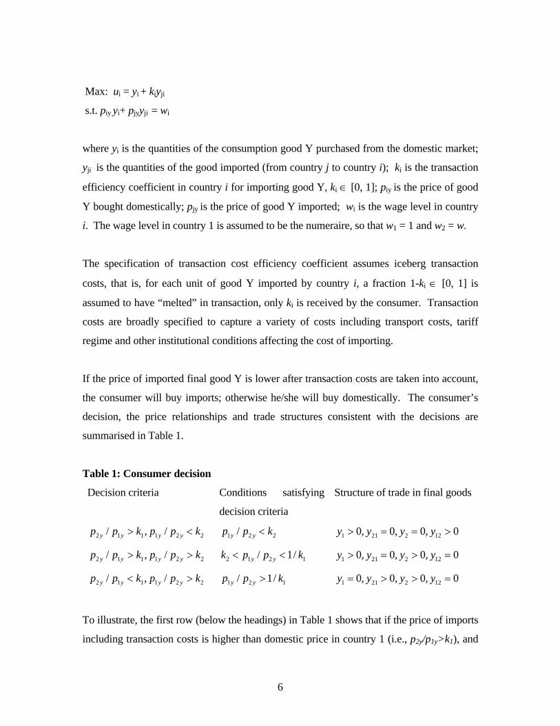
Max: ui = yi + kiyji

s.t. piy yi+ pjyyji = wi

where yi is the quantities of the consumption good Y purchased from the domestic market;

yji is the quantities of the good imported (from country j to country i); ki is the transaction

efficiency coefficient in country i for importing good Y, ki ∈ [0, 1]; piy is the price of good

Y bought domestically; pjy is the price of good Y imported; wi is the wage level in country

i. The wage level in country 1 is assumed to be the numeraire, so that w1 = 1 and w2 = w.

The specification of transaction cost efficiency coefficient assumes iceberg transaction

costs, that is, for each unit of good Y imported by country i, a fraction 1-ki ∈ [0, 1] is

assumed to have “melted” in transaction, only ki is received by the consumer. Transaction

costs are broadly specified to capture a variety of costs including transport costs, tariff

regime and other institutional conditions affecting the cost of importing.

If the price of imported final good Y is lower after transaction costs are taken into account,

the consumer will buy imports; otherwise he/she will buy domestically. The consumer’s

decision, the price relationships and trade structures consistent with the decisions are

summarised in Table 1.

Table 1: Consumer decision

Decision criteria Conditions satisfying

decision criteria

Structure of trade in final goods

2 1 1 1 2/ , /y y y yp p k p p k> < 2 2 1 2/y yp p k< 1 21 2 120, 0, 0, 0y y y y> = = >

2 1 1 1 2/ , /y y y yp p k p p k> > 2 1 2 1 2/ 1/y yk p p k< < 1 21 2 120, 0, 0, 0y y y y> = > =

2 1 1 1 2/ , /y y y yp p k p p k< > 2 1 1 2/ 1/y yp p k> 1 21 2 120, 0, 0, 0y y y y= > > =

To illustrate, the first row (below the headings) in Table 1 shows that if the price of imports

including transaction costs is higher than domestic price in country 1 (i.e., p2y/p1y>k1), and

6

if the price of imports including transaction costs is lower than domestic price in country 2

(i.e., p1y/p2y<k2), then the relative price would satisfy the condition that p1y/p2y<k2. Under

this condition, consumers in country 1 will buy domestically (y1>0, y21 = 0), and consumers

in country 2 will buy imports (y2=0, y12 > 0).

Similarly the second row shows the situation where consumers in both countries choose to

buy domestically, and the third row shows the situation where consumers in country 1 buy

imports and those in country 2 buy domestically.

2.2. Firm decision

2.2.1 Production of the final good

A final-good producing firm makes two decisions: whether to vertically integrate into the

production of intermediate good X, and where to source good X.

If the firm chooses to vertically integrate, it can produce the intermediate good X either in

its home country or overseas, or both. If it chooses to produce overseas, an internal

transaction cost will be incurred. The internal transaction cost includes the transport cost

and other cost associated with intra-firm importation of intermediate goods. The

production function of good Y for the representative vertically integrated firm in country i

is:

yi = aiy(xiv+tivxjiv)β Liy1-β

where aiy is the productivity coefficient in country i which captures the productivity

difference in producing good Y between the two countries; xiv is the quantity of

intermediate good X produced domestically and xjiv is that produced overseas by the

vertically integrated firm in country i; tiv (tiv <1) is the internal transaction efficiency

7

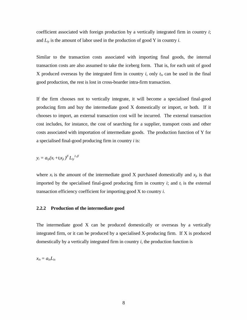
coefficient associated with foreign production by a vertically integrated firm in country i;

and Liy is the amount of labor used in the production of good Y in country i.

Similar to the transaction costs associated with importing final goods, the internal

transaction costs are also assumed to take the iceberg form. That is, for each unit of good

X produced overseas by the integrated firm in country i, only tiv can be used in the final

good production, the rest is lost in cross-boarder intra-firm transaction.

If the firm chooses not to vertically integrate, it will become a specialised final-good

producing firm and buy the intermediate good X domestically or import, or both. If it

chooses to import, an external transaction cost will be incurred. The external transaction

cost includes, for instance, the cost of searching for a supplier, transport costs and other

costs associated with importation of intermediate goods. The production function of Y for

a specialised final-good producing firm in country i is:

yi = aiy(xi +tixji )β Liy

1-β

where xi is the amount of the intermediate good X purchased domestically and xji is that

imported by the specialised final-good producing firm in country i; and ti is the external

transaction efficiency coefficient for importing good X to country i.

2.2.2 Production of the intermediate good

The intermediate good X can be produced domestically or overseas by a vertically

integrated firm, or it can be produced by a specialised X-producing firm. If X is produced

domestically by a vertically integrated firm in country i, the production function is

xiv = aixLix

8

where aix is the labor productivity coefficient for a vertically integrated firm in country i

producing domestically; and Lix is the amount of labor in country i used in the production

of X.

If X is produced by a specialised X-producing firm in country i, the production function is

xi = bixLix

where bix is the labor productivity coefficient for a specialised X-producing firm in country

i.

If X is produced overseas by the vertically integrated firm, the production function is

xjiv = bjxLjx

where bjx is the labor productivity coefficient for a specialised firm in country j. This

specification assumes that if a vertically integrated firm sets up an input plant overseas, the

plant will have the same productivity as a local specialised X-producing firm.

Due to economies of specialisation, labor productivity in X production by a specialised

firm is assumed to be higher than that in a vertically integrated firm, i.e., aix<bix.

In deciding whether to vertically integrate and where to source the intermediate good X, a

Y-producing firm compares the unit costs of producing Y associated with different

structural forms of production. If a Y-producing firm in country i vertically integrates and

produces X domestically, the unit cost function for good Y can be obtained by solving the

cost minimisation problem:

min ( )i ix iyw L L+

1. . 1,iy iv iy iv ix ixs t a x L x a Lβ β− = =

9

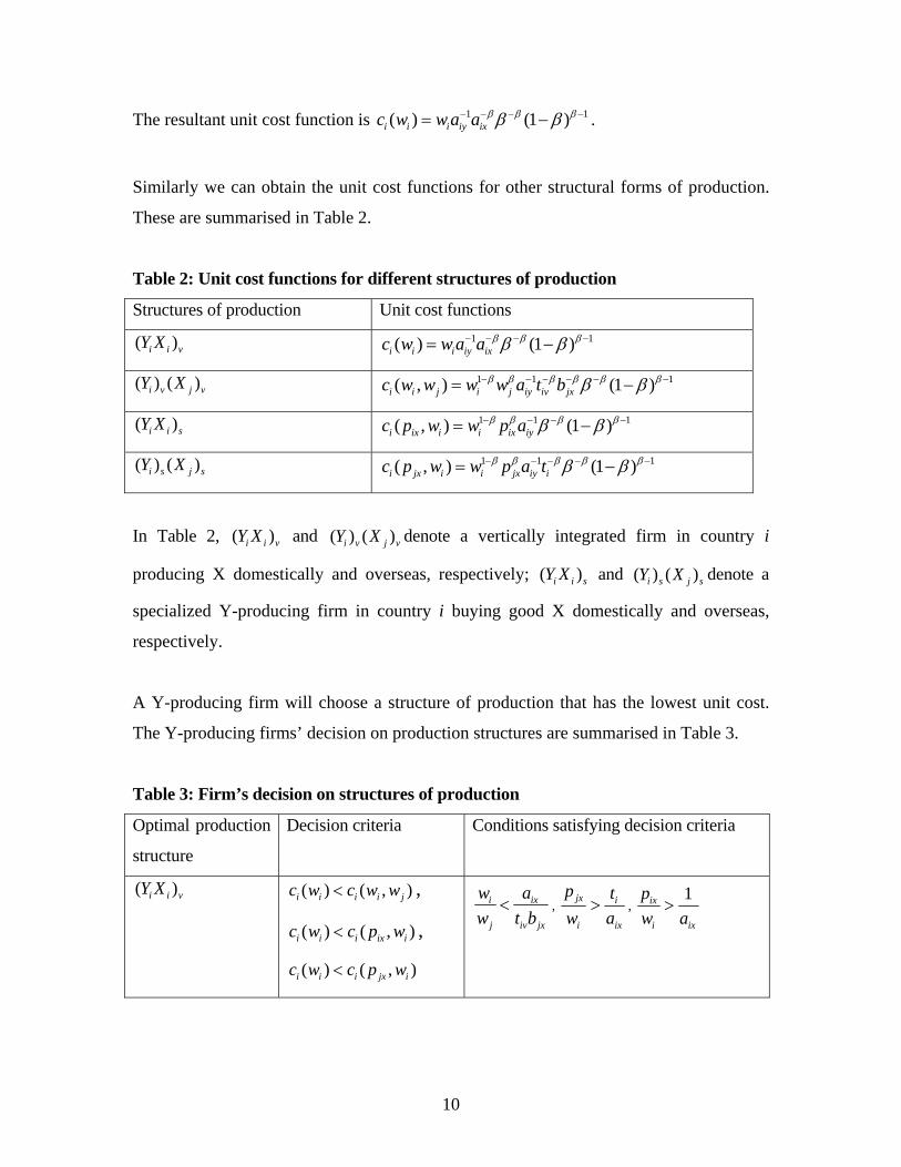
The resultant unit cost function is 1 1( ) (1 )i i i iy ixc w w a a β β ββ β− − − −= − .

Similarly we can obtain the unit cost functions for other structural forms of production.

These are summarised in Table 2.

Table 2: Unit cost functions for different structures of production

Structures of production Unit cost functions

( )i i vY X 1 1( ) (1 )i i i iy ixc w w a a β β ββ β− − − −= −

( ) ( )i v j vY X 1 1( , ) (1 )i i j i j iy iv jxc w w w w a t b 1β β β β β ββ β− − − − − −= −

( )i i sY X 1 1( , ) (1 )i ix i i ix iyc p w w p a 1β β ββ β β− − − −= −

( ) ( )i s j sY X 1 1( , ) (1 )i jx i i jx iy ic p w w p a tβ β β β ββ β 1− − − − −= −

In Table 2, and ( ) denote a vertically integrated firm in country i

producing X domestically and overseas, respectively; and ( ) denote a

specialized Y-producing firm in country i buying good X domestically and overseas,

respectively.

( )i i vY X ( )i v j vY X

( )i i sY X ( )i s j sY X

A Y-producing firm will choose a structure of production that has the lowest unit cost.

The Y-producing firms’ decision on production structures are summarised in Table 3.

Table 3: Firm’s decision on structures of production

Optimal production

structure

Decision criteria Conditions satisfying decision criteria

( )i i vY X ( ) ( , )i i i i jc w c w w< ,

( ) ( , )i i i ix ic w c p w< ,

( ) ( , )i i i jx ic w c p w<

i ix

j iv jx

w aw t b

< , jx i

i i

p tw a

>x

, 1ix

i ix

pw a

>

10

( ) ( )i v j vY X ( , ) ( )i i j i ic w w c w< ,

( , ) ( , )i i j i ix ic w w c p w< ,

( , ) ( , )i i j i jx ic w w c p w<

i ix

j iv j

w aw t b

>x

, jx i

j iv jx

p tw t b

> , 1ix

j iv jx

pw t b

>

( ) ( )i i v j vY X X ( , ) ( )i i j i ic w w c w= ,

( , ) ( , )i i j i ix ic w w c p w< ,

( , ) ( , )i i j i jx ic w w c p w<

i ix

j iv jx

w aw t b

= , jx i

j iv j

p tw t b

>x

, 1ix

j iv jx

pw t b

>

( )i i sY X ( , ) (i ix i i ic p w c w< ) ,

( , ) ( , )i ix i i i jc p w c w w< ,

( , ) ( , )i ix i i jx ic p w c p w<

1ix

jx i

pp t

< , 1ix

j iv jx

pw t b

< , 1ix

i ix

pw a

<

( ) ( )i s j sY X ( , ) (i jx i i ic p w c w< )

)

,

( , ) ( ,i jx i i i jc p w c w w< ,

( , ) ( ,i jx i i ix ic p w c p w )<

jx i

j iv jx

p tw t b

< , jx i

i i

p tw a

<x

, jx

iix

pt

p<

( ) ( )i i s j sY X X ( , ) (i jx i i ic p w c w< )

)

,

( , ) ( ,i jx i i i jc p w c w w< ,

( , ) ( ,i jx i i ix ic p w c p w )=

jx i

j iv jx

p tw t b

< , jx i

i i

p tw a

<x

, jx

iix

pt

p=

Compared to Table 2, Table 3 includes two additional production structures: structure

denotes a vertically integrated firm produces X both domestically and

overseas, and structure denotes a specialised firm buys X both domestically

and overseas. The first structure is chosen when the costs of producing domestically and

overseas are the same, and the second structure chosen when the costs of buying

domestically and overseas are the same.

( ) ( )i i v j vY X X

( ) ( )i i s j sY X X

2.3. Possible trade structures

11

Combining consumer decisions and firm decisions in both countries (see Table 1 and

Table 3 above), we can identify a set of trade structures that can occur in equilibrium and

corresponding conditions that satisfy the optimisation of both consumer and firm

decisions. These are summarised in Table 4.

Table 4: Trade structures and corresponding conditions

Conditions for

optimal consumption

pattern

Conditions for optimal production structure Trade structure

11

2 1 2

x

v x

aww t b

> , 2 1

2 1 2

x

v x

p tw t b

> , 1

2 1 2

1x

v x

pw t b

> 1 2( ) ( )v vY X

11

2 1 2

x

v x

aww t b

= , 2 1

2 1 2

x

v x

p tw t b

> , 1

2 1 2

1x

v x

pw t b

> 1 1 2( ) (v vY X X )

2 1

2 1 2

x

v x

p tw t b

< , 2 1

1 1

x

x

p tw a

< , 21

1

x

x

p tp

< 1 2( ) ( )s sY X

12

2

y

y

pk

p<

2 1

2 1 2

x

v x

p tw t b

< , 2 1

1 1

x

x

p tw a

< , 21

1

x

x

p tp

= 1 1 1( ) ( )s sY X X

11

2 1 2

x

v x

aww t b

< , 2 1

1 1

x

x

p tw a

> , 1

1 1

1x

x

pw a

>

22

1 2 1

x

v x

aww t b

< , 2

2 2

1x

x

pw a

> , 1 2

2 2

x

x

p tw a

>1 1 2 2( ) ( )v vY X Y X

11

2 1 2

x

v x

aww t b

< , 2 1

1 1

x

x

p tw a

> , 1

1 1

1x

x

pw a

>

12

2

x

x

p tp

> , 2

2 2

1x

x

pw a

< , 2

1 2 1

1x

v x

pw t b

<

1 1 2 2( ) ( )v sY X Y X

12

2 1

1y

y

pk

p k< <

11

2

x

x

p tp

< , 1

2 1 2

1x

v x

pw t b

< , 1

1 1

1x

x

pw a

<

22

1 2 1

x

v x

aww t b

< , 2

2 2

1x

x

pw a

> , 1 2

2 2

x

x

p tw a

>1 1 2 2( ) ( )s vY X Y X

12

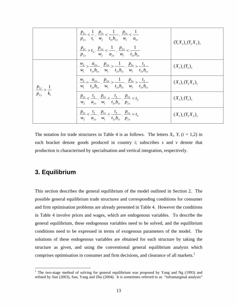
1

2 1

1x

x

pp t

< , 1

2 1 2

1x

v x

pw t b

< , 1

1 1

1x

x

pw a

<

12

2

x

x

p tp

> , 2

2 2

1x

x

pw a

< , 2

1 2 1

1x

v x

pw t b

<1 1 2 2( ) ( )s sY X Y X

22

1 2 1

x

v x

aww t b

> , 2

1 2 1

1x

v x

pw t b

> , 1 2

1 2 1

x

v x

p tw t b

> 1 2( ) ( )v vX Y

22

1 2 1

x

v x

aww t b

= , 2

1 2 1

1x

v x

pw t b

> , 1 2

1 2 1

x

v x

p tw t b

> 1 2 2( ) ( )v vX Y X

1 2

2 2

x

x

p tw a

< , 1 2

1 2 1

x

v x

p tw t b

< , 12

2

x

x

p tp

< 1 2( ) ( )s sX Y

1

2 1

1y

y

pp k

>

1 2

2 2

x

x

p tw a

< , 1 2

1 2 1

x

v x

p tw t b

< , 12

2

x

x

p tp

= 1 2 2( ) ( )s sX Y X

The notation for trade structures in Table 4 is as follows. The letters Xi, Yi (i = 1,2) in

each bracket denote goods produced in country i; subscribes s and v denote that

production is characterised by specialisation and vertical integration, respectively.

3. Equilibrium

This section describes the general equilibrium of the model outlined in Section 2. The

possible general equilibrium trade structures and corresponding conditions for consumer

and firm optimisation problems are already presented in Table 4. However the conditions

in Table 4 involve prices and wages, which are endogenous variables. To describe the

general equilibrium, these endogenous variables need to be solved, and the equilibrium

conditions need to be expressed in terms of exogenous parameters of the model. The

solutions of these endogenous variables are obtained for each structure by taking the

structure as given, and using the conventional general equilibrium analysis which

comprises optimisation in consumer and firm decisions, and clearance of all markets.1

1 The two-stage method of solving for general equilibrium was proposed by Yang and Ng (1993) and refined by Sun (2003), Sun, Yang and Zhu (2004). It is sometimes referred to as “inframarginal analysis”

13

To illustrate, consider structure 1 2( ) ( )s sY X . In this structure, firms in country 1 specialise

in producing good Y, they import the intermediate good X from specialised X-producers

in country 2, and export the final good Y.

First we look at consumer decision. Given this structure, a representative consumer in

country 2 buys good Y domestically, i.e., y21 = 0, thus the consumer decision problem

simplifies to

Max: 1 1u y=

s.t. 1 1 1yp y w=

Solving this problem gives us the demand function for good Y in country 1, which is

11

1

d

y

wyp

=

In contrast, a representative consumer in country 2 only buys imports, i.e., y2=0, thus the

consumer decision problem simplifies to

Max: 2 2 1u k y= 2

s.t. 1 12 2yp y w=

Solving this problems gives us the demand function for good Y in country 2, which is

212

1

d

y

wyp

=

as the method comprises an “infra-marginal” stage of identifying economic structures and corresponding conditions using the Kuhn-Tucker conditions of consumer and firm optimisation problems, as well as the standard stage of marginal analysis which solves for the equilibrium prices and quantities for each economic structure.

14

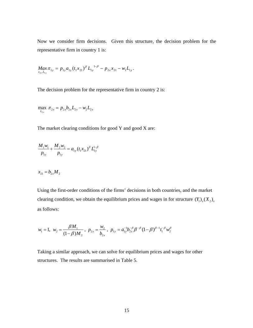
Now we consider firm decisions. Given this structure, the decision problem for the

representative firm in country 1 is:

yxyyyyLxLwxpLxtapMax

y11212

11211111,

)(121

−−= −ββπ .

The decision problem for the representative firm in country 2 is:

22 2 2 2 2max

xx x x xL 2xp b L w Lπ = −

The market clearing conditions for good Y and good X are:

11 1 2 21 1 21 1

1 1

( )y yy y

M w M w a t x Lp p

β β−+ =

21 2 2xx b M=

Using the first-order conditions of the firms’ decisions in both countries, and the market

clearing condition, we obtain the equilibrium prices and wages in for structure 1 2( ) ( )s sY X

as follows:

1 1,w = 12

2(1 )Mw

Mββ

=−

, 22

2x

x

wpb

= , 1 11 1 2 1(1 )y y x 2p a b t wβ β β ββ β− − − − −= − β

Taking a similar approach, we can solve for equilibrium prices and wages for other

structures. The results are summarised in Table 5.

15

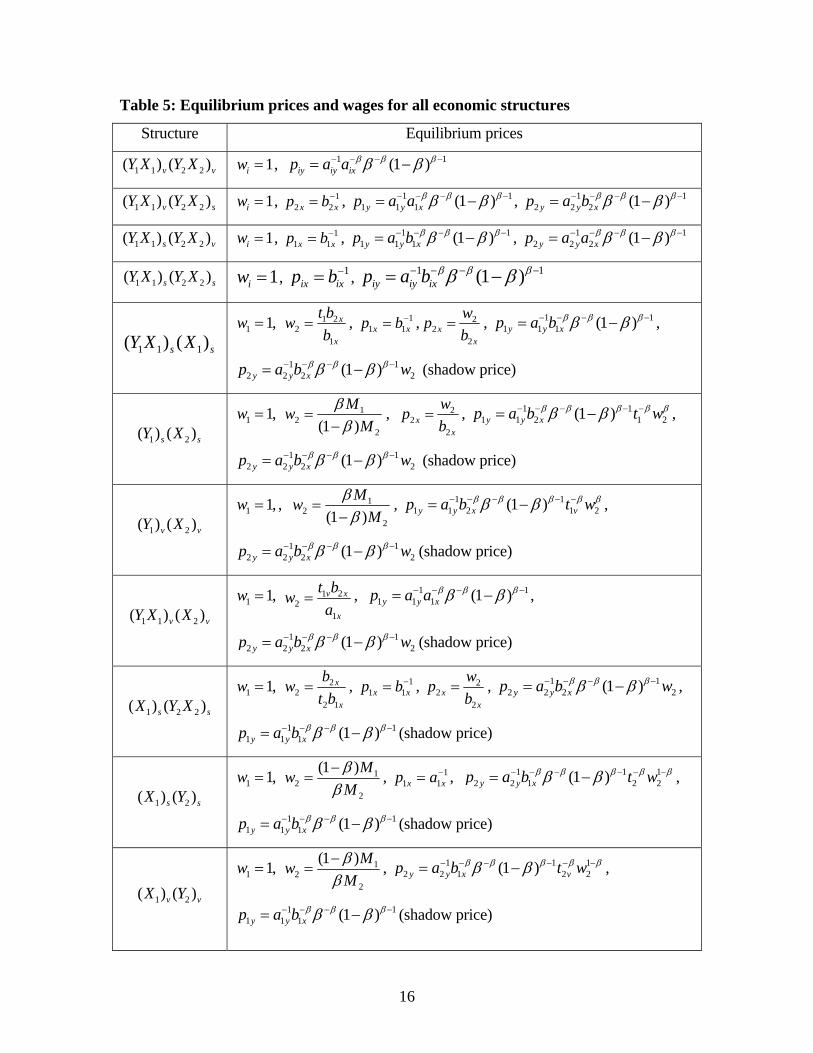
Table 5: Equilibrium prices and wages for all economic structures

Structure Equilibrium prices

1 1 2 2( ) (v vY X Y X ) 1iw = , 1 1(1 )iy iy ixp a a β β ββ β− − − −= −

1 1 2 2( ) (v sY X Y X ) 1iw = , 12 2x xp b−= , 1 1

1 1 1 (1 )y y xp a a β β ββ β− − − −= − , 1 12 2 2 (1 )y y xp a b β β ββ β− − − −= −

1 1 2 2( ) ( )s vY X Y X 1iw = , 11 1x xp b−= , 1 1

1 1 1 (1 )y y xp a b β β ββ β− − − −= − , 1 12 2 2 (1 )y y xp a a β β ββ β− − − −= −

1 1 2 2( ) ( )s sY X Y X 1iw = , 1ix ixp b−= , 1 1(1 )iy iy ixp a b β β ββ β− − − −= −

1 1 1( ) ( )s sY X X 1 1,w = 1 2

21

x

x

t bwb

= , 11 1x xp b−= , 2

22

xx

wpb

= , 1 11 1 1 (1 )y y xp a b β β ββ β− − − −= − ,

12 2 2 (1 )y y x

12p a b wβ β ββ β− − − −= − (shadow price)

1 2( ) ( )s sY X 1 1,w = 1

22(1 )

MwM

ββ

=−

, 22

2x

x

wpb

= , 1 11 1 2 1(1 )y y x 2p a b t wβ β β ββ β− − − − −= − β

12

,

12 2 2 (1 )y y xp a b wβ β ββ β− − − −= − (shadow price)

1 2( ) ( )v vY X 1 1,w = , 1

22(1 )

MwM

ββ

=−

, 1 11 1 2 1(1 )y y x v 2p a b t wβ β β ββ β− − − − −= − β

12

,

12 2 2 (1 )y y xp a b wβ β ββ β− − − −= − (shadow price)

1 1 2( ) (v vY X X ) 1 1,w = 1 2

21

v x

x

t bwa

= , 1 11 1 1 (1 )y y xp a a β β ββ β− − − −= − ,

12 2 2 (1 )y y x

12p a b wβ β ββ β− − − −= − (shadow price)

1 2 2( ) ( )s sX Y X 1 1,w = 2

22 1

x

x

bwt b

= , 11 1x xp b−= , 2

22

xx

wpb

= , 1 12 2 2 (1 )y y x 2p a b wβ β ββ β− − − −= − ,

11 1 1 (1 )y y xp a b β β ββ β− − − −= − 1 (shadow price)

1 2( ) ( )s sX Y 1 1,w = 1

22

(1 )MwMβ

β−

= , 11 1x xp a−= , 1 1

2 2 1 2 2(1 )y y x1p a b t wβ β β ββ β β− − − − − −= − ,

11 1 1 (1 )y y xp a b β β ββ β− − − −= − 1 (shadow price)

1 2( ) ( )v vX Y 1 1,w = 1

22

(1 )MwMβ

β−

= , 1 12 2 1 2 2(1 )y y x v

1p a b t wβ β β ββ β β− − − − − −= − ,

11 1 1 (1 )y y xp a b β β ββ β− − − −= − 1 (shadow price)

16

1 2 2( ) ( )v vX Y X 1 1,w = 2

22 1

x

v x

awt b

= , 1 12 2 2 (1 )y y x 2p a a wβ β ββ β− − − −= − ,

11 1 1 (1 )y y xp a b β β ββ β− − − −= − 1 (shadow price)

In some of the structures where good Y is not produced domestically in one country,

there is no actual domestic price for Y in that country. We have calculated a “shadow”

domestic price of Y for that structure, which is the price that would be if Y were to be

produced domestically.2 The shadow prices are information required for consumer

decisions as to whether to buy domestically or abroad (refer to Table 1).

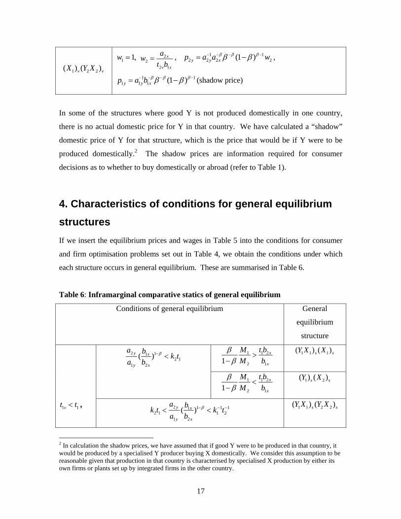
4. Characteristics of conditions for general equilibrium structures If we insert the equilibrium prices and wages in Table 5 into the conditions for consumer

and firm optimisation problems set out in Table 4, we obtain the conditions under which

each structure occurs in general equilibrium. These are summarised in Table 6.

Table 6: Inframarginal comparative statics of general equilibrium

Conditions of general equilibrium General

equilibrium

structure

1 21

2 11x

x

t bMM b

ββ

>−

1 1 1( ) ( )s sY X X 2 112 1

1 2

( )y x

y x

a b k ta b

β− <

1 21

2 11x

x

t bMM b

ββ

<−

1 2( ) ( )s sY X

1 1vt t< , 2 1k t 2 1 1 11

1 21 2

( )y x

y x

a b k ta b

β− − −< <)

1 1 2 2( ) (s sY X Y X

2 In calculation the shadow prices, we have assumed that if good Y were to be produced in that country, it would be produced by a specialised Y producer buying X domestically. We consider this assumption to be reasonable given that production in that country is characterised by specialised X production by either its own firms or plants set up by integrated firms in the other country.

17

21

2 2 1

1 x

x

bMM t b

ββ−

> 1 2( ) ( )s sX Y 2 2vt t< 2 1 111 2

1 2

( )y x

y x

a b k ta b

β− −> 1−

21

2 2 1

1 x

x

bMM t b

ββ−

< 1 2 2( ) ( )s sX Y X

1 21

2 11v x

x

t bMM a

ββ

>−

1 1 2( ) (v vY X X ) 2 112 1

1 2

( )y xv

y x

a a k ta b

β− <

1 21

2 11v x

x

t bMM a

ββ

<−

1 2( ) ( )v vY X

2 1vk t 2 1 1 111 2

1 2

( )y xv

y x

a a k ta b

β− − −< <)

1 1 2 2( ) (s sY X Y X

21

2 2 1

1 x

v x

aMM t b

ββ−

< 1 2 2( ) ( )v vX Y X

1 1vt t> ,

2 2vt t> 2 1 111 2

1 2

( )y xv

y x

a a k ta b

β− −> 1−

21

2 2 1

1 x

v x

aMM t b

ββ−

> 1 2( ) ( )v vX Y

21 21

2 1 11x

x

t bMM t b

ββ

>−

1 1 2( ) ( )s sY X X 2 112 1

1 2

( )y x

y x

a b k ta a

β− <

21 21

2 1 11x

x

t bMM t b

ββ

<−

1 2( ) ( )s sY X

2 1k t 2 1 1 111 2

1 2

( )y xv

y x

a b k ta a

β− − −< <)

1 1 2 2( ) (s sY X Y X

21

2 2 1

1 x

v x

aMM t b

ββ−

< 1 2 2( ) ( )v vX Y X

1 1vt t< ,

2 2vt t>

2 1 111 2

1 2

( )y xv

y x

a b k ta a

β− −> 1−

21

2 2 1

1 x

v x

aMM t b

ββ−

> 1 2( ) ( )v vX Y

1 21

2 11v x

x

t bMM a

ββ

>−

1 1 2( ) (v vY X X ) 2 112 1

1 2

( )y xv

y x

a a k ta b

β− <

1 21

2 11v x

x

t bMM a

ββ

<−

1 2( ) ( )s sY X

1 1vt t> , 2 1vk t 2 1 1 11

1 21 2

( )y x

y x

a a k ta b

β− − −< <)

1 1 2 2( ) (s sY X Y X

18

2 21

2 12 1

1 x

x

t bMM t b

ββ−

> 1 2( ) ( )s sX Y 2 2vt t< 2 1 111 2

1 2

( )y x

y x

a a k ta b

β− −> 1−

2 21

2 12 1

1 x

x

t bMM t b

ββ−

< 1 2 2( ) ( )s sX Y X

Note that the conditions of general equilibrium in effect partition the fifteenth dimension

parameter space ( M, ,ix iy ixa a b 1, M2, β, t1, t2, t1v, t2v, k1, k2) into subsets. Within each

parameter subset, a specific economic structure emerges as the general equilibrium

structure. For instance, the first row of Table 6 means that within the subset defined by

, , 1 1vt t< 2 2vt t< 2 112 1

1 2

( )y x

y x

a b k ta b

β− < and 1 21

2 11x

x

t bMM b

ββ

>−

, the structure 1 1 1( ) ( )s sY X X will

emerge as the general equilibrium structure.

It can be seen from Table 6 that 9 different economic structures each with different

consumption, production and trade patterns can emerge in general equilibrium, these

structures are:

(1) the autarky structure 1 1 2 2( ) ( )s sY X Y X , in which both countries produce both good

X and good Y in specialised firms; there is no international trade. Note that

vertical integration cannot be a general equilibrium autarky structure because we

assume the productivity of X in a specialised firm is higher than an integrated

firm, and that there is zero domestic transaction cost in trading good X in the

domestic market or internal control cost in producing X domestically. In other

words, there is no trade-off between economies of specialisation and low

transaction costs, thus specialisation will be the dominant choice that occurs in

equilibrium with no international trade.

(2) The global outsourcing structures 1 2( ) ( )s sY X and 1 2( ) ( )s sX Y , in which firms in

country 1 and country 2, respectively, specialise in producing Y and outsource the

intermediate good X globally.

19

(3) The FDI structures and1 2( ) ( )vY X v v1 2( ) ( )vX Y , in which firms in country 1 and

country, respectively, vertically integrate into X production and set up overseas

plants to produce good X.

(4) The mixed specialised structures 1 1 1( ) ( )s sY X X and 1 2 2( ) ( )s sX Y X , in which firms in

country 1 and country 2, respectively, specialise in producing Y and outsource

good X both domestically and globally.

(5) The missed vertical structures and1 1 2( ) (v vY X X ) v1 2 2( ) ( )vX Y X , in which firms in

country 1 and country 2, respectively, vertically integrate into X production and

produce good X both domestically and overseas.

Which structure will occur in general equilibrium depends on which subsets the parameters

fall into. Each parameter subset is defined in terms of technological comparative

advantage in producing goods Y and X between the two countries ( 2 1 1 1

1 2 2 2

, , ,y x x x

y x x

a b a ba b b a x

),

intensity of intermediate good X used in the production of good ( β ), transaction

efficiency associated with international trade in good Y (k1, k2), internal transaction

efficiency associated with producing X overseas by a vertically integrated firm (t1v, t2v),

external transaction efficiency associated with importing good X (t1, t2), and relative

population size ( 1

2

MM

).

The interactions of the parameters are complex, however, some general conclusions can

be drawn from the results presented in Table 6. The first conclusion is the general

statement that the general equilibrium structure is determined by the interaction of

parameters, specifically, we have

Proposition 1 Depending on the values of parameters, different economic structures can

occur in general equilibrium. The general equilibrium structure may involve autarky

where there is international trade in neither final goods nor intermediate goods; or

20

specialised final good producers engaging in global outsourcing or both domestic and

global outsourcing of intermediate good; or vertically integrated producers engaging in

global production (through FDI) or both of domestic and global production of

intermediate good.

Note that in Table 6 the first column compares the internal transaction efficiency of a

vertically integrated firm and the external transaction efficiency of a specialised firm. It

is clear from Table 6 that when internal transaction efficiency is lower than external

transaction efficiency in a country (tiv<ti), firms in that country do not choose vertical

integration in general equilibrium. For instance, the first block of 5 structures in Table 6

are all characterised by firms in country 1 being specialised producers of X and or Y.

Thus we have

Proposition 2 The choice between vertical integration and specialised production of

final goods depends on the relative size of the internal transaction efficiency associated

with vertical integration and external transaction efficiency associated with specialised

production. Ceteris paribus, an increase in external transaction efficiency increases the

likelihood that specialised production of final goods occurs in general equilibrium.

It should be noted that our model assumes zero transaction costs in domestic trading, that

is the domestic transactions efficiency of good X is one. Thus the trade-off between

vertical integration and specialisation characterised in proposition 2 is more precisely the

trade-off between vertically integration with production of good X overseas, and the

specialisation with good X imported.3 Nevertheless, Proposition 2 still captures the idea

put forward by Cheung (1983) that the boundary of the firm is determined by the relative

transaction efficiency in trading intermediate goods (external transaction efficiency in our

model) and the transaction cost of hiring labor to produce the intermediate goods

internally (internal transaction efficiency in our model).

3 If we introduce transaction costs in domestic trade and production in both countries, the definition of parameter subsets will be more complex as there will be four additional parameters. However the general conclusions of the model will be the same except that 3 additional autarky structures may emerge which are characterised by at least one country vertically integrating into X production.

21

The second column of Table 6 describes each country’s comparative advantage in

relation to the two goods X and Y, taking into account different types of transaction

costs. Notice that due to positive transaction costs, international trade does not always

occur in equilibrium. However if international trade does occur in equilibrium, the

direction of trade flow in our model is consistent with Ricardo’s theory of comparative

advantage, which predicts that a country will export the good it has comparative

advantage in producing. For instance, the first cell of column 2 indicates that country 2

has comparative advantage in good X, the corresponding equilibrium structures are

characterised by country 2 exporting good X. Thus we have

Proposition 3 If the extent of comparative advantage is not sufficient to outweigh the

transaction costs associated with international trade, the general equilibrium structure

will be autarky. If comparative advantage is sufficiently large such that international

trade occurs in equilibrium, then the direction of trade flow will be such that each

trading country exports the good that it has a comparative advantage in producing.

Proposition 3 highlights a distinct feature of our model, which is its ability to endogenize

the emergence of international trade as well as the consumption and trade pattern and

production organisations.

Finally, the third column of Table 6 is a measure of the relative production capacity of

the intermediate good between the two countries. The relative production capacity is

determined by the relative size of the labor force, relative productivity in X production

and the intensity of X used in the production of Y. From the results in Table 6, we get

Proposition 4 If the production capacities of the intermediate good in the two countries

are balanced, complete international specialisation (i.e., each country producing only

one good) may occur in equilibrium. If the production capacities are out of balance, the

country with a larger capacity will produce both goods in equilibrium and the

22

equilibrium structure will involve the larger country either outsourcing both domestically

and abroad, or producing the intermediate good both domestically and overseas.

5. Conclusion

In this paper we have developed a general equilibrium model of domestic and global

sourcing. The model adapts the traditional Ricardian model of international trade to

analyse production and trade in intermediate goods, and introduces three types of

transaction costs to the model: the transaction costs associated with international trade in

final goods, the external transaction costs associated with international outsourcing of

intermediate goods, and the internal transaction costs associated with overseas production

of intermediate goods by vertically integrated firms. Our model endogenises the

decision as to whether or not to vertically integrate and the location of intermediate good

production. It also endogenises the emergence of international trade in equilibrium.

The main conclusions of our model are summarised in four propositions. In summary

form, our model suggests that (1) depending on parameter values, different equilibrium

structures may occur in general equilibrium; (2) the choice between vertical integration

and specialisation depends on the comparison or relative sizes of external transaction

costs of outsourcing and internal transaction costs of production; (3) international trade

will occur in equilibrium if the extent of comparative advantage outweighs the

transaction costs of international trade. The direction of trade flow will be such that each

country exports the good it has comparative advantage in; and (4) complete international

specialisation is possible if the production capacities of the trading countries are

balanced; otherwise the country with a larger capacity will produce both goods

domestically.

Despite the relative simplicity in the logical structure of our model, the model is able to

derive a rich set of conclusions. This suggests to us that the underlying structure of the

traditional Ricardian model is a powerful tool for analyzing a wide range of issues in

23

international trade. For instance, our model can be extended to include different types of

labor to analyze the impact of international outsourcing on wage dispersion between

skilled and unskilled labor. A further extension is to introduce the difference in labor

market institutions to the model and investigate how labor market institutions interact

with international trade to affect wages for skilled and unskilled labor.

References Abraham, Katharine G., and Susan K. Taylor (1996), “Firm’s use of outside contractors,

theory and evidence”, Journal of Labor Economics, 14, 394-424.

Antras, Pol and Helpman, Elhana (2004), “Global Sourcing”, Journal of Political

Economy, 112(3), 552-580.

Cheung, Steven (1983), “The Contractual Nature of the Firm”, The Journal of Law and

Economics, 1, 1-21.

Coase, Ronald (1937), “The Nature of the Firm”, Economica, 4, 386-405.

Deardorff, Alan V. (2001), “Fragmentation in simple trade models”, North American

Journal of Economics and Finance, 12, 121-137.

Feenstra, Robert C. (1998), “ Integration of Trade and Disintegration of Production in the

Global Economy”, Journal of Economic Perspectives, 12 (4), 31-50.

Grossman, Gene M; Helpman, Elhanan (2002), “Integration versus Outsourcing in

Industry Equilibrium”, The Quarterly Journal of Economics, 117 (1), 85-120.

Grossman, Gene M; Helpman, Elhanan (2005), “Outsourcing in a Global Economy”,

Review of Economic Studies, 72(1), 135-159.

24

Grossman, Sanford and Hart, Oliver (1986), “The Costs and Benefits of Ownership: A

Theory of Vertical and Lateral Integration”, Journal of Political Economy, 94, 691-719.

Hummels, David, Jun Ishii, and Kei-Mu Yi (2001), “The nature and growth of vertical

specialization in world trade”, Journal of International Economics, 54, 75-96.

Kohler, Wilhelm (2001), “A specific-factors view on outsourcing”, North American

Journal of Economics and Finance, 12, 31-53.

Sun, Guang-Zhen (2003), “Identification of Equilibrium Structures of Endogenous

Specialisation: A Unified Approach Exemplified,” in Yew-Kwang Ng, He-Ling Shi, and

Guang-Zhen Sun, eds., The Economics of e-Commerce and Networking Decisions:

Applications and Extensions of Inframarginal Analysis. London: Palgrave Macmillan, pp.

195-213.

Sun, Guang-Zhen; Yang, Xiaokai and Zhou, L. (2004), “General Equilibria in Large

Economies with Endogenous Structure of the Division of Labor.” Journal of Economic

Behavior and Organization, 55(2), 237-256.

Williamson, Oliver E. (1975), Markets and Hierarchies: Analysis and Antitrust

Implications, New York, NY: Free Press.

Williamson, Oliver E (1985), The Economic Institutions of Capitalism, New York, NY:

Free Press.

Yang, Xiaokai and Yew-Kwang Ng (1993), Specialisation and Economic Organisation,

a New Classical Microeconomic Framework, Amsterdam: North-Holland.

Yang, Xiaokai and Yew-Kwang Ng (1995), “Theory of the firm and structure of residual

rights”, Journal of Economic Behavior and Organisation, 26, 107-128.

25