Moment estimation in discrete shifting level model applied to fast array-CGH segmentation A. Gandolfi* Dipartimento di Matematica U. Dini, Università di Firenze, Viale Morgagni 67/A, 50134 Florence, Italy M. Benelli Dipartimento di Matematica U. Dini, Università di Firenze, Viale Morgagni 67/A, 50134 Florence, Italy and Center for the Study of Complex Dynamics (CSDC), University of Florence, Florence, Italy A. Magi Dipartimento di Matematica U. Dini, Università di Firenze, Viale Morgagni 67/A, 50134 Florence, Italy and Diagnostic Genetic Unit, Careggi University Hospital, 50134 Florence, Italy S. Chiti Dipartimento di Matematica U. Dini, Università di Firenze, Viale Morgagni 67/A, 50134 Florence, Italy We develop a mathematical theory needed for moment estimation of the parameters in a general shifting level process (SLP) treating, in particular, the finite state space case geometric finite normal (GFN) SLP. For the SLP, we give expressions for the moment estimators together with asymptotic (co)variances, following, completing, and correcting CLINE (Journal of Applied Probability 20, 1983, 322–337); formulae are then made more explicit for the GFN-SLP. To illustrate the potential uses, we then apply the moment estimation method to a GFN-SLP model of array comparative genomic hybridization data. We obtain encouraging results in the sense that a segmentation based on the estimated parameters turns out to be faster than with other currently available methods, while being comparable in terms of sensitivity and specificity. Keywords and Phrases: shifting level process, moment estimator, array-CGH, finite state space, segmentation, confidence intervals, DNA, microarray. 1 Introduction We develop here a mathematical theory related to moment estimations of the param- eters in a shifting level process (SLP) or shifting level model (Chernoff and Zacks, *gandolfi@math.unifi.it © 2013 The Authors. Statistica Neerlandica © 2013 VVS. Published by Wiley Publishing, 9600 Garsington Road, Oxford OX4 2DQ, UK and 350 Main Street, Malden, MA 02148, USA. Statistica Neerlandica (2013) Vol. 67, nr. 3, pp. 227–262 doi:10.1111/stan.12005 227 brought to you by CORE View metadata, citation and similar papers at core.ac.uk provided by Florence Research

Welcome message from author
This document is posted to help you gain knowledge. Please leave a comment to let me know what you think about it! Share it to your friends and learn new things together.
Transcript

Moment estimation in discrete shifting levelmodel applied to fast array-CGH segmentation
A. Gandolfi*
Dipartimento di Matematica U. Dini, Università di Firenze, Viale Morgagni67/A, 50134 Florence, Italy
M. Benelli
Dipartimento di Matematica U. Dini, Università di Firenze, Viale Morgagni67/A, 50134 Florence, Italy and Center for the Study of Complex
Dynamics (CSDC), University of Florence, Florence, Italy
A. Magi
Dipartimento di Matematica U. Dini, Università di Firenze, Viale Morgagni67/A, 50134 Florence, Italy and Diagnostic Genetic Unit, Careggi
University Hospital, 50134 Florence, Italy
S. Chiti
Dipartimento di Matematica U. Dini, Università di Firenze, Viale Morgagni67/A, 50134 Florence, Italy
We develop a mathematical theory needed for moment estimation ofthe parameters in a general shifting level process (SLP) treating, inparticular, the finite state space case geometric finite normal (GFN)SLP. For the SLP, we give expressions for the moment estimatorstogether with asymptotic (co)variances, following, completing, andcorrecting CLINE (Journal of Applied Probability 20, 1983, 322–337);formulae are then made more explicit for the GFN-SLP. To illustratethe potential uses, we then apply the moment estimation method to aGFN-SLP model of array comparative genomic hybridization data. Weobtain encouraging results in the sense that a segmentation based onthe estimated parameters turns out to be faster than with other currentlyavailable methods, while being comparable in terms of sensitivity andspecificity.
Keywords and Phrases: shifting level process, moment estimator,array-CGH, finite state space, segmentation, confidence intervals,DNA, microarray.
1 Introduction
We develop here a mathematical theory related to moment estimations of the param-eters in a shifting level process (SLP) or shifting level model (Chernoff and Zacks,
*[email protected]© 2013 The Authors. Statistica Neerlandica © 2013 VVS.Published by Wiley Publishing, 9600 Garsington Road, Oxford OX4 2DQ, UK and 350 Main Street, Malden, MA 02148, USA.
Statistica Neerlandica (2013) Vol. 67, nr. 3, pp. 227–262doi:10.1111/stan.12005
227
brought to you by COREView metadata, citation and similar papers at core.ac.uk
provided by Florence Research

1964; Salas and Boes, 1980). In the a mathematical paper on such moment estima-tion, CLINE (1983) considered a general SLP Y ¼ Yaf g1a¼1, constructed as a concate-nation of segments of random length, randomly selected from a family of processes(all of the mechanisms describing such randomness being identified as the underlyingprocesses), and derives, under very general conditions, asymptotic properties of theempirical moments
1aS fa ¼ 1
a
Xai¼1
f Yi;Yiþ1 . . . ;Yiþkð Þ
with f : Xkþ1 ! RP . In particular, CLINE (1983) managed to derive, under suitablebut very general conditions, a law of large numbers and a central limit theorem(CLT) for 1
aSfa as functions of the moments of the underlying processes. In Section 2
and Appendix A, we recall Cline’s main results, obtaining then more explicit andreadable formulae when f is a polynomial (which amounts to all what is neededin our intended main application) and correcting two mistakes in Cline’s paper(Appendix B).CLINE (1983) then specialized to an SLP with geometrically distributed segment
lengths and other underlying processes being normal (a geometric normal normal orGNN-SLP), and provides, without showing the very long calculations, explicit formu-lae for asymptotic moments and their (co)variances.Here, instead, we specialize in a different direction, namely to a geometric finite
normal shifting level process or GFN-SLP, in which segment lengths are still geomet-rically distributed and errors are normally distributed, but the state space is finite. Forsuch case, we obtain more explicit formulae in Section 3 for the asymptotics of theempirical moments. Detailed calculations are demonstrated in the Appendix, wherewe also correct two errors in Cline’s paper. In particular, we manage to invert theasymptotic expressions in Lemma 2 for the first moments and 2-autocovariancesand 3-autocovariances as functions of the model parameters. This allows to explicitlydetermine moment estimators and their asymptotic (co)variances. These are the mainresults of this paper.To illustrate the potential applications of the moment estimations in the GFN-SLP,
we consider the segmentation problem in array comparative genomic hybridization(array-CGH) data.Array-CGH (OOSTLANDER, MEIJER and YLSTRA (2004)) is a microarray tech-
nique that allows detection and mapping of genomic alterations (see CARTER
(2007)). Test and reference DNA are differently fluorescent labeled, arrays of clonesare accurately spotted (following human genome) onto glass slides, and then themixed fluorescent DNA is hybridized to the array. The resulting fluorescent ratio isthen measured, clone by clone, with measurements affected by a non-negligible noise;currently, one array can contain up to 106 probes, each of the order of 20–100monomers(LIU (2007)). A function (the log base 2) of the fluorescent ratio is then plotted asfunction of the clone number, giving a discrete time jump process. In the
228 A. Gandolfi et al.
© 2013 The Authors. Statistica Neerlandica © 2013 VVS.

subsequent array-CGH analysis, one needs to detect the breakpoints where thereis DNA copy-number variations (CNVs) and then identify for each connected region thecopy number, calling neutral for the physiological two copies, loss for less, and gain formorecopies. The task is complicated by the high level of noise in the measurement process,which confuses short segments with CNV with a noisy but physiologically normal tract.After several segmentation methods have been devised (HUPE et al. 2004; PICARD
et al. 2005; OLSHEN et al. 2004; MYERS et al. 2004), in MAGI et al. (2010), the GNNversion of the SLP (GNN-SLP) has been successfully used to model and analyzearray-CGH data. In the approach of MAGI et al. (2010), array-CGH data aremodeled by a GNN-SLP, and the analysis consists of assigning a preliminarysegmentation and then carrying out an iterative approach similar to the pseudo-expectation–maximization algorithm for hidden Markov models (HMMs) FORTIN
and KEHAGIAS (2006): a partly iterative estimation of number of states and modelparameters (FORNEY (1973)) is performed in the E step and, finally, the best seg-mentation is obtained in the M step by using the Viterbi algorithm. The E and Msteps are repeated until an identical result is obtained. The algorithm is approximatelyquadratic in the number of probes, and, although it is not yet the case, this might turnout to be a critical issue as the number of probes is dramatically increasing withtechnological advances.We follow here a similar approach, which is presented in Section 5. However, we
start in Section 4 by noticing that the state space of the SLP is not arbitrary, as itreflects the possible values of (the log of) the fluorescent ratio of DNA copy numberagainst normal; such ratio can only be 0,1/2,1,3/2,. . ., with some noise due to thecolor reading mechanism, and occasional minor alterations due to genetic reasons.Notice that level 1 reflects normality. By these remarks, the state space of theSLP contains only few rather well-determined values, which can be separatelydetermined at the start of the analysis, possibly using previous genetic informa-tion; to avoid missing unusual values, it is also possible to include extra states(as long as this does not burden running time, this has no lasting effect asprobabilities estimations permit to identify irrelevant states). We are thenmodeling the array-CGH data as an SLP with geometric waiting time (G)between switches, a finite distribution (F) over the previously identified states,and a normal independent noise (N) with constant variance. This amounts to aGFN-SLP, as described in Section 4.In Section 5, we describe how to apply our method to the segmentation problem
in array-CGH. Starting from the fixed set of possible states, we obtain the modelparameters by using the moment estimators, and then we can apply just one step ofthe Viterbi algorithm to obtain a segmentation. The detailed theory of momentestimation, which we develop in this paper, would allow also to determine confidenceintervals (CI): we only give one example in Section 5, as the evaluation of the error inasymptotic approximation requires more investigation.We then report the results of systematic comparisons of the segmentation based on
moment estimation with some other currently used segmentation methods. Tests are
GFN-SLP moment estimation 229
© 2013 The Authors. Statistica Neerlandica © 2013 VVS.

performed using synthetic chromosomes generated by LAI et al. (2005). In Section 6,we compare the receiver operating characteristic (ROC) curves generated by ourmethod (with several different choices for the initial state) with those of othermethods, and find that they are comparable.In Section 7, we compare the execution times, revealing that the moment segmen-
tation is faster than the other methods.The results on the proposed method are thus extremely encouraging, in particular
because the rapid growth of microarray size and resolution requires segmentationalgorithms with high computational performance.An additional issue, raised by an anonymous reviewer of the manuscript, concerns
the normality assumption for the noise. In this work, the normality is assumed as itappears to be a good approximation for normalized read counts data; see YOON
et al. (2009); on the other hand, it is conceivable that other distributions could bemore adequate. As the crucial mathematical step in our procedure is Lemma 2, whichshows that the map from parameters to statistics is continuously invertible, it wouldbe interesting to find general conditions for the noise distribution under which suchinvertibility is ensured.
2 Results for general SLP
In this section, we recall the definition of SLP together with some results from CLINE
(1983); we then write some general expressions of useful moments.Let X;Xð Þ, Λ;Lð Þ, and N;Nð Þ be measurable spaces, with N= {1, 2, 3 . . .}, and let
Ω;F ; Pð Þ be the underlying probability space.
Definition 1. If X lð Þj
n o1
j¼1; l 2 Λ
� �is a family of stochastic processes on Ω;F ; Pð Þ
with elements in X, and Nn;Λnf g1n¼1 is a stochastic process in Ω;F ; Pð Þ with elementsin N�Λ, then the process
Yaf g1a¼1 ¼ X Λ1ð Þ1 ;X Λ1ð Þ
2 ; . . . ;X Λ1ð ÞN1
;X Λ2ð Þ1 ; . . . ;X Λ2ð Þ
N2;X Λ3ð Þ
1 ; . . .n o
¼ X Λnð Þj
n oNn
j¼1
� �1
n¼1
(1)
is called a Shifting Level Process or SLP with epochs ‘shift’ Tnf g1n¼1 ¼N1 þ . . .þNnf g1n¼1, levels Λnf g1n¼1, and underlying process X lð Þ
j
n o1
j¼1; l 2 Λ.
See CLINE (1983) for comments on the definition. The SLP generally depends onthe parameters in the distributions of the Xj’s and Nn;Λnf g1n¼1 , which can beestimated through the observable process Yaf g1a¼1 . Notice that for all a2ℕ, the
random variable Ya takes value in X, so that if f : Xkþ1 ! R, the sample moments are
1aS fa ¼ 1
a
Xai¼1
f Yi;Yiþ1; . . . ;Yiþkð Þ: (2)
230 A. Gandolfi et al.
© 2013 The Authors. Statistica Neerlandica © 2013 VVS.

As mentioned in CLINE (1983), we only consider real-valued sample moments asthe results are easily extended to vector-valued or continuous functions of the samplemoments. The main estimation results will be expressed in terms of the auxiliary,unobservable random variables
Rfn ¼
XTn
i¼Tn�1þ1
f Yi; . . . ;Yiþkð Þ ¼XNn
j¼1
f X Λnð Þj ;X
Ljþ1ð ÞIjþ1
; . . . ;XLjþkð Þ
Ijþk
� �
where
Lj ¼ Λmj
Ij ¼ j � Tmj � Tn
� �and mj satisfies
Tmj � Tn
� �< j ≤ Tmjþ1 � Tn
� �:
For instance, if f : X3 ! R, then
Rfn ¼
XNn�2
j¼1
f X Λnð Þj ;X Λnð Þ
jþ1 ;X Λnð Þjþ2
� þ f X Λnð Þ
Nn�1;X Λnð Þ
Nn;X Λnþ1ð Þ
1
� þf X Λnð Þ
Nn;X Λnþ1ð Þ
1 ;X LNnþ2ð ÞINnþ2
� :
(3)
For later convenience, we indicate
f nð Þj ¼ f X Λnð Þ
j ;XLjþ1ð Þ
Ijþ1; . . . ;X
Ljþkð ÞIjþk
� �
and
Ufn ¼
Xnj¼1
R fj :
CLINE (1983) presented some general sufficient conditions for the law of largenumbers and the CLT for 1
aSfa . We recall here Corollaries 2.1 and 3.1 only, as they
are enough to deal with the discrete version used in the applications discussed later.It is these results that are used by Cline in the second part of his paper, where thereare some errors corrected in Appendix B:
Proposition 1. (Corollary 2.3 in CLINE (1983)). Let Yaf g ¼ X Λnð Þj
n oNn
j¼1
� �be an SLP
such that
1. {Nn, Λn} is a sequence of random elements in N�Λ with P[Λn=Λm] = 0, n 6¼m.
GFN-SLP moment estimation 231
© 2013 The Authors. Statistica Neerlandica © 2013 VVS.

2. X lð Þj
n o, l 2 Λ is a family of independent stochastic processes and independent
of {Nn, Λn}.
Let f : Xkþ1 ! R and define Rfn and Sf
a as before.
1. If {Nn, Λn} is stationary, ergodic and E[Nn] = �<1, E Rfn
� ¼ �θ < 1, then1=að ÞS f
a ! θ a.s.2. If {Nn, Λn} is l-dependent and E[Nn]! �, E R f
n
�! �θ , E R fj jn
h i! �z , and
V R fn
�≤Knb, V R fj j
n
h i≤Knb, V[Nn]≤Kn
b, b< 1, then 1=að ÞS fa ! θ a.s.
Proposition 2. (Corollary 3.1 in CLINE (1983)). Let Yaf g ¼ X Λnð Þj
n oNn
j¼1
� �be an SLP
and f : Xkþ1 ! R be such that:
1. {Nn,Λn} is a strictly stationary, #-mixing of random elements in N�Λ with P[Λn=Λm] = 0 for n 6¼m and
X1j¼1
# jð Þ1=2 < 1.
2. X lð Þj
n o, l2Λ is a family of independent stochastic processes and independent
of {Nn,Λn}3. V Rf
n
�< 1, V[Nn]<1, V R f�θj j
n
h i< 1.
If
� ¼ E Nn½ �;�θ ¼ E Rf
n
�;
�wj ¼ Cov Rfn � θNn;R
fnþj � θNnþj
h i; j≥0
then
ffiffiffia
p 1aSfa � θ
� �! N 0; g2
� �in distribution; (4)
where
g2 ¼ w0 þ 2X1j¼1
wj : (5)
The preceding two results express the asymptotic values of the sample moments interms of the moments of Nn andRf
n. In turn, CLINE (1983) provided in Section 4 some
formulae without derivation for the moments ofRfn in terms of the moments ofNn and
f X Λnð Þ1 ; . . .
� , provided that enough moments of f exist, but these are not directly
computable in explicit examples as the moments of f require some careful directcomputation depending on their different arguments. We give here some more
232 A. Gandolfi et al.
© 2013 The Authors. Statistica Neerlandica © 2013 VVS.

explicit and directly computable formulae for the moments ofRfn, for polynomial f, in
terms of the moments of Nn and the join moments of the X Λnð Þi ’s. This makes the
derivation and verification of explicit expression much easier.We now derive various formulae under the following hypothesis:
1. X lð Þj
n o, l 2 Λ, is a family of independent stochastic processes, each of which is
a sequence of exchangeable random elements of X.2. {Nn} and {Λn} are sequences of i.i.d. random elements of N and Λ, respec-
tively, and are independent of each other and of X lð Þj
n o.
The limit theorems require computing the moments of Rfn. We compute them for
f x1 . . . ; xrð Þð Þ ¼Yr
l¼1xhll in terms of the moments of Nn and of those of X lð Þ
j
n o:
1. ai ¼ E Nin
�,
2. bi lð Þ ¼ E X lð Þj
� i �, and
3. mi=E[li];
the last expression is not used in the first results below. Note that bi(l) arerandom variables, and actually, the formulae are functions of the expected valuesof products of the bi(l)’s. Later, when we consider X lð Þ
j
n oto be normally distrib-
uted, we can substitute such expected values by formulae depending only on themoments of {Λn}.We start with f : X ! R, that is, f(x) = xh. At the price of additional complications
in the formulae, we could deal with any analytic f, but we avoid such details here asthey are not needed in the main applications below. Let
Sk;r ¼ f k1; . . . ; kr; s1; . . . ; srð Þ : ki 2 N; si 2 N; 1≤ k1 < k2 < . . . < kr≤ k;Xri¼1
kisi ¼ kg:
and
Sk;r;Nn ¼ f k1; . . . ; kr; s1; . . . ; srð Þ 2 Sk;r : s ¼Xri¼1
si ≤Nng:
Then we have the following:
Theorem 1.
E Rxhn
� k �¼Xkr¼1
Xk1;...;kr;s1;...;srð Þ2Sk;r;Nn
k!k1!ð Þs1 �...� kr!ð Þsrð Þ s1!�...�sr!ð Þ
�E bs1k1h � . . . � bsrkrh
h ias þ
Xs�1
m¼1
as�m �1ð ÞmX
1≤i1<...<im≤ s�1
Ymj¼1
ij
!:
GFN-SLP moment estimation 233
© 2013 The Authors. Statistica Neerlandica © 2013 VVS.

Proof
E Rxhn
� k �¼ E
XNn
i¼1
X lð Þi
� h !k24
35
¼ E
"Xkr¼1
Xk1;...;kr;s1;...;srð Þ2Sk;r
k!k1!ð Þs1 � . . . � kr!ð Þsrð Þ s1!� . . . �sr!ð ÞX
i1;...;is2 1;...;Nnf g; diffferentX1 lð Þ
i
� hk1 � . . . � X lð Þis1
� hk1X lð Þ
is1þ1
� hk2
� . . . � X lð Þis1þs2
� hk2 � . . . � X lð Þis1þs2þ...sr�1þ1
� hkr � . . . � X lð Þis
� hkr#
¼Xkr¼1
Xk1;...;kr;s1;...;srð Þ2Sk;r
k!k1!ð Þs1 � . . . � kr!ð Þsrð Þ s1!� . . . �sr!ð Þ
�E bs1k1h� . . . �bsrkrhh i
E Nn Nn � 1ð Þ� . . . � Nn � sþ 1ð Þ½ �
¼Xkr¼1
Xk1;...;kr;s1;...;srð Þ2Sk;r;Nn
k!k1!ð Þs1 � . . . � kr!ð Þsrð Þ s1!� . . . �sr!ð Þ
�E bs1k1h� . . . �bsrkrhh i
as þXs�1
m¼1
as�m �1ð ÞmX
1≤ i1<...<im ≤ s�1
Ymj¼1
ij
!
where the third equality holds as the Xli ’s are conditionally independent given l, the
number of i1, . . ., is2 {1, . . .,Nn}, different from each other, is Nn(Nn� 1) � . . . � (Nn�s+1), and the variables Nn’s are also independent. The last equality holds asNn(Nn� 1) � . . . � (Nn� s+ 1) = 0 for s>Nn. □
For the GNN model considered in CLINE (1983), ai is the ith moment of a geomet-ric random variable with parameter p, bi(l) is the ith moment of a N(l, (1�r)s2)distribution, and l is itself N(m, rs2) with ith moment mi. The four parameters ofthe model, r, s, m, and p, satisfy
rs2 ¼ m2 � m211� rð Þs2 ¼ E b2 lð Þ½ � � E b1 lð Þ½ �ð Þ2m ¼ m1p ¼ a�1
8>><>>:
from which we obtain their expression in terms of the moments b1, b2, m1, m2, and a:
s2 ¼ E b2 lð Þ½ � � E b1 lð Þ½ �ð Þ2 þ m2 � m21
r ¼ m2 � m21E b2 lð Þ½ � � E b1 lð Þ½ �ð Þ2 þ m2 � m21m ¼ m1
p ¼ a�1
:
8>>>><>>>>:
Then with the preceding formulae, it is easy to recompute (see Cline (1983) p. 334)for the function f(x) = x
234 A. Gandolfi et al.
© 2013 The Authors. Statistica Neerlandica © 2013 VVS.
E Rxn
� ¼ E b1 lð Þ½ �a1 ¼ E l½ � 1p¼ 1
pm
V Rxn � mNn
� ¼ E Rxn � mNn
� �2h i¼ E Rx
n
� �2h i� 2mE NnRx
n
�þ m2E Nnð Þ2h i
¼ E½ b2 lð Þð �a1 þ E b1 lð Þð Þ2h i
a2 � a1ð Þ � 2ma2E b1 lð Þ½ � þ m2a2
¼ E l2 þ 1� rð Þs2 �a1 þ E l2
�a2 � a1ð Þ � 2ma2E l½ � þ m2a2
¼ 1� rð Þs2
pþ m2 þ rs2� � 2� p
p2� m2
2� pp2
¼ 1ps2 þ 2
1� pp2
rs2;
and for f(x) = x2 (denoted by f0 in CLINE (1983))
E Rx2n
h i¼ 1
ps2 þ m2� �
V Rx2n � s2 þ m2
� �Nn
h i¼ E Rx2
n
� 2 �� 2 s2 þ m2� �
E NnRx2n
h iþ s2 þ m2� �2
E Nnð Þ2h i
¼ m2 þ 1� rð Þs2� �2a21 � 2 s2 þ m2
� �a2 m2 þ 1� rð Þs2� �þ a2 s2 þ m2
� �2¼ 1
p2s4 þ 4m2s2� �þ 2
1� pp2
2r2s4 þ 4rm2s2� �
:
3 The GFN-SLP model
We now specialize to another particular SLP: the geometric finite normal or GFN-
SLP. In the GFN-SLP, {Nn}� i.i.d. geometric (p); given l, X lf gn
n o� i.i.d. N(l,t2);
and {Λn}� i.i.d. with a finite distribution on {b1, . . .,bT} with parametersp={p1, . . .,pT}; all processes being independent. To avoid trivialities and simplifythe later formulae, we assume T> 1 and p< 1, which is to say, that {Yi} is notindependent. The GFN-SLP is simple enough that Propositions 1 and 2 apply. Inparticular, ai’s, bi’s, and mi’s can be explicitly written in terms of the parameters ofthe model. In fact, we have a1 = 1/p, a2 ¼ 2�p
p2 ,
bi lð Þ ¼Xbi=2cj¼0
rj ið Þli�2jt2j;
the ith moment of a normal (l, t2) distribution, for which there exist explicitexpressions for the rj(i); and, finally, mi= mi(p1, . . .,pT) is the ith moment of the finitedistribution of the {Λn}’s.We now intend to estimate the T+1 parameters p1, . . ., pT� 1, p and t2; for conve-
nience, we consider the T+2 parameters p, p, and t2 subject to the constraintP
i pi=1.The statistics used will be sample moments of the form given in (2) for the functionsf(x) =xi, f1(x1,x2) =x1 � x2, and f2(x1,x2,x3) =x1 � x2 � x3. More precisely, we use
GFN-SLP moment estimation 235
© 2013 The Authors. Statistica Neerlandica © 2013 VVS.

mi ¼ 1nSxin ; i ¼ 1; . . . ;T � 1
mf1 ¼1nSx1�x2n
mf2 ¼1nSx1�x3n :
(6)
The next lemma computes the asymptotics of the statistics in terms of the modelparameters, together with the asymptotic variances. Then the subsequent lemmashows how to explicitly invert such asymptotics to retrieve the model parameters;the final theorem gives the explicit form of the parameter estimators with theirasymptotic variance.
Lemma 1. If Yaf g ¼ X Λnð Þj
n oNn
j¼1
� �is a GFN-SLM, then for all i=1, . . .,T� 1
mi ¼ 1nSxin ! mi :¼
Xbi=2cj¼0
rj ið Þmi�2jt2j a:s: (7)
and
ffiffiffin
p 1nSxin �mi
� �! N 0; g2i
� �in distribution;
where
g2i ¼1a1
E Rxin
� 2 �� a2m2
i
�¼ 1
a1a2 � a1ð ÞE b2i lð Þ �þ a1m2i � a2m2
i
�:
Moreover,
mf1 ¼1nSf1n ! mf1 :¼
1a1
a1 � 1ð Þm2 þ m21 � ¼ 1
a1a1 � 1ð Þ m2 � t2
� �þm21
�a:s:
and
ffiffiffin
p 1nS f 1n �mf1
� �! N 0; g2f1
� in distribution;
where
g2f1 ¼1a1
(a2 � 2a1 þ 1ð Þm4 þ 2a2 � 7a1 � 2pþ 6þ a2
a21
� �t4
þ 2a1 � a2 � 1þ a2a21
� �m2
2 þ 12a1 � 4a2 þ 2p� 8� 2a2a21
� �m2t2
þ a2a21
� 4
� �m4
1 þ 4 a1 � 1ð Þm1m3 þ 2 4� 2a1 � a2a21
� �m2m
21
�2 4a1 þ p� 4� a2a21
� �m2
1t2
�:
236 A. Gandolfi et al.
© 2013 The Authors. Statistica Neerlandica © 2013 VVS.
Finally,
mf 2 ¼1nSf2n ! mf2 :¼
1a1
a1 � 2þ pð Þm2 þ 2� pð Þm21 �
¼ 1a1
a1 � 2þ pð Þ m2 � t2� �þ 2� pð Þm2
1
�a:s:
and ffiffiffin
p 1nSf2n �mf2
� �! N 0; g2f2
� in distribution;
where
g2f2 ¼1a1
(a2 � 4a1 þ 4� pð Þm4
þ 2a2 � 11a1 � 2 p3 � 5p2 þ 9p� 8� �þ 2� pð Þ2 a2
a21þ 2p 2� pð Þ 1
a1
�t4
þ 4a1 � a2 þ 2p2 � 3p� 4þ 2p 2� pð Þ 1a1
þ 2� pð Þ2 a2a21
�m2
2
þ2 10a1 � 2a2 þ p3 � 6p2 þ 12p� 12� 2p 2� pð Þ 1a1
� 2� pð Þ2 a2a21
�m2t2
þ 2 p2 þ 4p� 8� �þ 2p 2� pð Þ 1
a1þ 2� pð Þ2 a2
a21
�m4
1 þ 8 a1 þ p� 2½ �m1m3
�2 4a1 þ 2 p2 þ 3p� 8� �þ 2p 2� pð Þ 1
a1þ 2� pð Þ2 a2
a21
�m2m
21
�2 8a1 þ p3 � 6p2 þ 12p� 12� 2p 2� pð Þ 1a1
� 2� pð Þ2 a2a21
�m2
1t2g:
Notice that, by the definition in (7), the vectors {m1, . . .,mT� 1} and {m1, . . ., mT� 1}are linked by a linear transformation. We actually use the vectorsm={1,m1, . . .,mT� 1}and m={1,m1, . . .,mT� 1}, which are related by
m ¼ Ut2 �mwith Ut2 a T�T lower triangular matrix depending on t2 of the form
Ut2 ¼1 0 0 0 . . .0 1 0 0 . . .t2 0 1 0 . . .. . .
2664
3775:
More explicitly, one obtains from (7)
mi ¼Xi‘¼0
I ‘¼i mod2ð Þri�‘2ið Þti�‘m‘ ¼
Xi‘¼0
Ut2 i; ‘½ �m‘ (8)
for i=1, . . .,T� 1, where IA indicates the indicator function of A. The matrixUt2 canbe inverted, and the explicit inverse relations we will use in the following asymptotictheory are
GFN-SLP moment estimation 237
© 2013 The Authors. Statistica Neerlandica © 2013 VVS.

m1 ¼ m1
m2 ¼ m2 � t2
m3 ¼ m3 � 3m1t2
m4 ¼ m4 � 6m2t2 þ 3t4:
Proof. The a.s. convergence of mi , for i=1, . . .,T� 1, mf 1 , and mf2 follows fromProposition 1. It is only needed to compute an explicit expression for θxi , which iseasily obtained from Theorem 1 with k=1: for all i=1, . . .,T� 1
θxi ¼ E Rxin
h i=E Nn½ � ¼ E bi lð Þ½ �
¼ EXbi=2cj¼0
rj ið Þli�2jt2j !
¼Xi=2j¼0
rj ið Þmi�2jt2j
!¼ mi:
The corresponding expressions for θf1 and θf2 can be computed from the formulaefor generic moments of functions f : X2 ! R and f : X3 ! R (see Appendix A),respectively. Using the relationship between m and m, we obtain
θf1 ¼ E Rf1n
�=E Nn½ � ¼ 1
a1a1 � 1ð ÞE b21 lð Þ �þ E b1 lð Þ½ �ð Þ2
h i
¼ 1a1
a1 � 1ð ÞE l2 �þ E l½ �ð Þ2
h i¼ 1
a1a1 � 1ð Þm2 þ m2
1
�¼ 1
a1a1 � 1ð Þ m2 � t2
� �þm21
�θf2 ¼ E Rf2
n
�=E Nn½ �
¼ 1a1
a1 � 2� pð ÞE b21 lð Þ �þ 1� pð Þ E b1 lð Þ½ �ð Þ2 þ p E b1 lð Þ½ �ð Þ2 þ 1� pð Þ E b1 lð Þ½ �ð Þ2h i
¼ 1a1
a1 � 2þ pð ÞE l2 �þ 2� pð Þ E l½ �ð Þ2
h i¼ 1
a1a1 � 2þ pð Þm2 þ 2� pð Þm2
1
�¼ 1
a1a1 � 2þ pð Þ m2 � t2
� �þ 2� pð Þm21
�:
The convergence in distribution of mi, for i=1, . . .,T� 1, mf1, and mf2 follows fromProposition 2, which also tells us how to calculate the variance of normal asymp-totic distribution.
238 A. Gandolfi et al.
© 2013 The Authors. Statistica Neerlandica © 2013 VVS.

The asymptotic variances mi’s can be computed from Theorem 1:
g2i ¼ w0 ¼V Rxi
n � θxiNn
h iE Nn½ �
¼ 1a1
E Rxin � θxiNn
� 2 �� E Rxi
n � θxiNn
h i� 2 �
¼ 1a1
E Rxin � θxiNn
� 2 � �
¼ 1a1
E Rxin
� 2 �þ θ2xiE N2
n
�� 2θxiE NnRxin
h i �
¼ 1a1
E Rxin
� 2 �þ a2m2
i � 2mia2E bi lð Þ½ � �
¼ 1a1
E Rxin
� 2 �� a2m2
i
�
¼ 1a1
a2 � a1ð ÞE b2i lð Þ �þ a1E b2i lð Þ½ � � a2m2i
�¼ 1
a1a2 � a1ð ÞE b2i lð Þ �þ a1m2i � a2m2
i
�:
The asymptotic variances g2f1 and g2f2 require long calculations, which are sketched inAppendix A. □
By the definition of the mi’s, m=V � p with V the Vandermonde matrix
V ¼1 1 1 . . .b1 b2 b3 . . .b21 b22 b23 . . .. . .
2664
3775 (9)
of size T�T. For vectors a and b, let (a,b) represent the concatenated vector. Then wecan invert first moments and 2-autocovariances and 3-autocovariances as functions ofthe model parameters:
Lemma 2. The RTþ2 ! RTþ2 map
p; p; t2� �! m; mf1 ;mf2
� �;
is invertible, and its inverse is given by the continuous functions:
p ¼ 1�mf2 �m21
mf1 �m21
(10)
t2 ¼ m2 �m21 �
mf1 �m21
� �2mf2 �m2
1
(11)
GFN-SLP moment estimation 239
© 2013 The Authors. Statistica Neerlandica © 2013 VVS.

p ¼ V�1U�1t2 m;mf1 ;mf2ð Þ�m: (12)
Proof The first two equalities are obtained by solving the system
mf1 ¼1a1
a1 � 1ð Þm2 þ m21
�mf2 ¼
1a1
a1 � 2þ pð Þm2 þ 2� pð Þm21
�8><>:
or, expressing the moments mi through sample moments mi,
mf1 ¼1a1
a1 � 1ð Þ m2 � t2� �þm2
1
�mf2 ¼
1a1
a1 � 2þ pð Þ m2 � t2� �þ 2� pð Þm2
1
�8><>:
with respect to the variable p and t2. Such inverses are continuous in the parameterrange of the model because mfi �m2
1 ¼ 1� pð Þi m2 � m21
� � 6¼ 0 for i=1, 2 being p 6¼ 1by hypothesis and the states variance different from zero by the model (otherwise, wewould have only one level).The vector p is obtained inverting the systemm ¼ Ut2m ¼ Ut2Vp. Such inverse exists
because U is a lower triangular matrix with all ones on the diagonal and V is aVandermonde matrix with elements bi 6¼ bj if i 6¼ j, for i, j= 1, . . .,T� 1, and it iscontinuous in the model parameters. □
The next theorem is the main result of our paper and gives the moment estimationof the model parameters:
Theorem 2. If Yaf g ¼ X Λnð Þj
n oNn
j¼1
� �is a GFN-SLM, then
pn ¼ 1� mf2 � m21
mf1 � m21
! p a:s: (13)
and ffiffiffin
ppn � pð Þ ! N 0; g2p
� �in distribution;
where
g2p ¼ JFC m1;...;mT�1ð ÞJtF 1; 1ð Þ
with
JF ¼
2m1 mf1 �mf2
� �mf1 �m2
1
� �2 0mf2 �m2
1
mf1 �m21
� �2 � 1mf1 �m2
1
� 2m1 mf1 �mf2
� �2mf2 �m2
1
� �2 1 � 2 mf1 �m21
� �mf2 �m2
1
mf1 �m21
� �2mf2 �m2
1
� �2
266664
377775:
and C m1;...;mT�1ð Þ explicitly calculable:
240 A. Gandolfi et al.
© 2013 The Authors. Statistica Neerlandica © 2013 VVS.

C m1;...;mT�1ð Þ t; rð Þ ¼ 1a1
a2 � a1ð ÞE bt lð Þbr lð Þ½ � þ a1mtþr � a2mtmrf g;
t2n ¼ m2 � m21 �
mf1 � m21
� �2mf2 � m2
1
! t2 a:s: (14)
and ffiffiffin
pt2n � t2�
! N 0; g2t2� �
in distribution;
whereg2t2 ¼ JFC m1;...; mT�1ð ÞJt
F 2; 2ð Þwith JF and C m1;...; mT�1ð Þ as above; finally,
pn ¼ V�1Ut2�1�mn ! p a:s: (15)
where mn ¼ 1; m1; . . . ; mT�1f g; and for t ¼ 1; . . . ;T
ffiffiffin
ppt � ptð Þ ! N 0; g2pt
� in distribution;
where
g2pt ¼ JGC m1;...;mT�1ð ÞJtG t; tð Þ
with C m1...;mT�1ð Þ as above and JG explicitly calculable in terms of the moments of thenormal distribution, as indicated in the proof.
Proof The a.e. convergences are simply a consequence of the a.e. convergence ofmn; mf1 ; mf2
� �to m; mf1 ;mf2
� �and the continuity of the functions in the previous Lemma.
By Lemma 1, we know the asymptotics of the statistics mn, mf1, and mf2 so that theasymptotic variances of the present theorem follow from a multidimensional deltamethod as follows. We evaluate all functions in the asymptotic values mn, mf1 , andmf2 of mn, mf1 , and mf2 .
In order to derive the asymptotic variances of p and t2, we consider the function
F : R4 ! R2
m1; m2; mf1 ; mf2
� �↦ pn ¼ 1� mf2 � m2
1
mf1 � m21
; p2n ¼ m2 � m2
1 �mf1 � m2
1
� �2mf2 � m2
1
!
whose Jacobian calculated in the asymptotic value of the vector m1; m2; mf 1 ; mf 2Þ�
isgiven by
JF ¼
2m1 mf1 �mf2
� �mf1 �m2
1
� �2 0mf2 �m2
1
mf1 �m21
� �2 � 1mf1 �m2
1
� 2m1 mf1 �mf2
� �2mf2 �m2
1
� �2 1 � 2 mf1 �m21
� �mf2 �m2
1
mf1 �m21
� �2mf2 �m2
1
� �2
266664
377775:
GFN-SLP moment estimation 241
© 2013 The Authors. Statistica Neerlandica © 2013 VVS.

If we denote with C m1;m2;mf1 ;mf2ð Þ the covariance matrix of the vectorm1; m2; mf1 ; mf2
� �, we have
C m1;m2;m f1 ;m f2ð Þ 1; 1ð Þ ¼ g21C m1;m2;m f1 ;m f2ð Þ 2; 2ð Þ ¼ g22C m1;m2;m f1 ;m f2ð Þ 3; 3ð Þ ¼ g2f1C m1;m2;m f1 ;m f2ð Þ 4; 4ð Þ ¼ g2f2
with the expression of the variances given in Lemma 1.The off-diagonal terms are explicitly computed in Appendix A.Using the multidimensional delta method, the variances of pand t2 are the diagonal
terms of the matrix JFCðm1m2mf1mf2
ÞJtF, that is
g2p ¼ 4m21 mf1 �mf2
� �2mf1 �m2
1
� �4 g21 þ4m1 mf1 �mf2
� �mf2 �m2
1
� �mf1 �m2
1
� �4 Cov m1; mf1
�
� 4m1 mf1 �mf2
� �mf1 �m2
1
� �3 Cov m1; mf2
�þ mf2 �m21
� �2mf1 �m2
1
� �4 g2f1� 2 mf2 �m2
1
� �mf1 �m2
1
� �3 Cov mf1 ; mf2
�þ 1
mf1 �m21
� �2 g2f2g2t2 ¼
4m21 mf1 �mf2
� �4mf2 �m2
1
� �4 g21 �4m1 mf1 �mf2
� �2mf2 �m2
1
� �2 Cov m1; m2½ �
þ 8m1 mf1 �mf2
� �2mf1 �m2
1
� �mf2 �m2
1
� �3 Cov m1; mf1
�
� 4m1 mf1 �mf2
� �2mf1 �m2
1
� �2mf2 �m2
1
� �4 Cov m1; mf2
�
þg22 �4 mf1 �m2
1
� �mf2 �m2
1
� � Cov m2; mf1
�þ 2 mf1 �m21
� �2mf2 �m2
1
� �2 Cov m2; mf2
�
þ 4 mf1 �m21
� �2mf2 �m2
1
� �2 g2f1 �4 mf1 �m2
1
� �3mf2 �m2
1
� �3 Cov mf1 ; mf2
�þ 4 mf1 �m21
� �4mf2 �m2
1
� �4 g2f2 :
For the variances vector g2p, we have to consider the function
G : RT�1 ! RT
m1; . . . ; mT�1ð Þ ↦ p¼ V�1U�1
t2m:
If we denote with JG the Jacobianmatrix of the functionG evaluated in (m1, . . .,mT� 1)and with C m1;...;mT�1ð Þ the variance–covariance matrix of the vector m1; . . . ; mT�1ð Þ ,
242 A. Gandolfi et al.
© 2013 The Authors. Statistica Neerlandica © 2013 VVS.
then the main diagonal of the matrix JGC m1;...;mT�1ð ÞJtG consists of the variances g2pt ,for t=1, . . .,T� 1.
Notice that for t=1, . . .,T� 1 we haveC m1;...;;mT�1ð Þ t; tð Þ ¼ g2t , whose expression isgiven in Lemma 1, whereas for t, r=1, . . .,T� 1 with t 6¼ r, we have
C m1...;mT�1ð Þ t; rð Þ ¼ Cov mt; mr½ �¼ 1
a1a2 � a1ð ÞE bt lð Þbr lð Þ½ � þ a1mtþr � a2mtmrf g:
□
We end this section by observing that the variances given by the previous theoremallow us to obtain CIs for segmentation parameters. Denoting by a the confidencelevel and considering the normal asymptotic distribution of estimators, we can derivethe following CIs for p, t2, and p, respectively:
pn � za=2
ffiffiffiffiffig2pn
r; pn þ za=2
ffiffiffiffiffig2pn
r !
t2n � za=2
ffiffiffiffiffiffig2t2n
s; t2n þ za=2
ffiffiffiffiffiffig2t2n
s0@
1A
pi � za=2
ffiffiffiffiffig2pin
s; pi þ za=2
ffiffiffiffiffig2pin
s0@
1A i ¼ 1; . . . ;T :
4 A discrete model for array-CGH data
Array-CGH is a microarray technology that allows one to detect and map geno-mic alterations. The goal of array-CGH analysis is to identify the boundaries ofthe regions where the number of DNA copies changes and then to label eachregion as loss, neutral, or gain. The genomic profile obtained from an array-CGH experiment can be considered as a signal made of noisy segments with dif-ferent lengths and with mean levels that shift their values according to the DNAcopy number.In the mathematical model of MAGI et al. (2010), this signal has been considered as
generated by the sum of two processes: a biological process due to a real variation ofthe number of DNA copies and a white noise process that mimics experimental error.We thus consider sequential observations Y= (Y1, . . .,YN) to be realizations of thesum of two independent stochastic processes:
Yi ¼ Λi þ ei
where ei is normally distributed white noise with variance t2, ei � N 0; s2e� �
, and Λi isthe unobserved mean level.
GFN-SLP moment estimation 243
© 2013 The Authors. Statistica Neerlandica © 2013 VVS.
In MAGI et al. (2010), the Λi’s have been taken to be normally distributed with thevalues taken in a specific sample estimated during the statistical analysis; however, wemake here the additional observation that these values are not arbitrary, as theyreflect the possible values of (the log of) the fluorescent ratio of DNA copy numberagainst absence of aberration. For deleted regions, the normalized log2-ratio islog2(1/2) =�1, whereas for amplified regions, the normalized log2-ratio is log2(3/2) = 0.5849 or log2(4/2) = 1 for four copies amplification. The value 0 corre-sponds to no aberrations. Hence, the possible states of Λi can be determined atthe start of the analysis and chosen to be taken from a finite distribution onb= {b1, . . .,bT} with parameters p= {p1, . . .,pT}. To avoid missing unusual values,one can, as we actually do, insert additional values of the bj’s with probability 0: this willbe recognized during the analysis and thus such states can be later removed. We thenbelieve that, as long as the relevant biologically justified values are considered, simplevariations in the choice of the vector b are not likely to alter the statistical analysis weare going to perform; we verified such claim with a systematic investigation of thesynthetic Lai et al. data set by using different choices of the state vector b (Section 6).
Then we consider the process X lð Þi
n o, whose elements are given by
X lð Þi ¼ lþ ei;
which corresponds to the process {Yi}, with the fixed value Λi= l. The randomvariables X lð Þ
i are i.i.d., and as the stochastic processes Λi and ei are independent,we obtain that E[Yi] =E[Λi] = m1, Var[Yi] =V[Λi] + t2, and consequently
E X lð Þi
h i¼ l
V X lð Þi
h i¼ t2;
therefore,
X lð Þi � N l; t2
� �:
Sequences of observations of given lengths with the same mean correspond tochromosomal aberrations, and their lengths Ni’s have been taken in MAGI et al.(2010) to be i.i.d. geometrically distributed stochastic process Ni � G pð Þ, withmean p, independent from the Λj’s and ej’s. As pointed out by an anonymousreferee, this might not be a very appropriate model in a number of cases inwhich high amplitude gains are often of small genomic size: in such a case,the Ni’s would no longer be identically distributed and the parameter p shoulddepend on Λi. However, this is not case in various other situations, includingprimarily cancer genomic analysis (Bayani et al. (2007)). In addition to this,the assumption of constant p simplifies the mathematical analysis while produc-ing very good results in terms of segmentation (Section 6). For these reasons,we stick to the assumption that the Ni’s are i.i.d. with Ni � G pð Þ. A more general
244 A. Gandolfi et al.
© 2013 The Authors. Statistica Neerlandica © 2013 VVS.

method of moments than the one described here could very likely be able todeal with varying p’s, but this requires extensions of the mathematical results,and we are currently investigating such possibility.With the assumptions made so far, the data originated by an array-CGH experi-
ment can be described through the GFN-SLP with
Nif g � G pð Þ i:i:d:
Λif g � F p1; . . . ; pTð Þ i:i:d:
X lð Þi
n o� N l; t2ð Þ i:i:d:
where the processes are mutually independent.
5 GFN-SLP analysis and segmentation of array-CGH data
From the results of the previous sections, we have an algorithm to estimate theparameter vector {p,p,t2} = {p,p1, . . .,pT,t
2} of the aforementioned model onceassigned the state vector {b1, . . .,bT}. The main difference with existing estimationmethods is that we can estimate all the parameters {p,p1, . . .,pT,t
2} in one step,whereas most methods require assigning some of the parameters and often neediterative steps. For this reason, our method is likely to be faster than any othercurrently available algorithm (Section 7).Collecting formulae for reader’s convenience, the method consists of evaluating
mi ¼ 1nSxin ; i ¼ 1; . . . ;T � 1
mf1 ¼1nSx1�x2n
mf2 ¼1nSx1�x3n :
as in (6) and mn ¼ 1; m1; . . . ; mT�1f g from the data. Then the GFN-SLP parameterestimators based on the method of moments are
p ¼ 1� mf2 � m21
mf1�m21
from (13),
t2¼ m2 � m21 �
mf1 � m21
� �2mf2 �m2
1
from (14) and
p ¼ V�1Ut2�1�mn
from (15) with Ut2 from (8) and V from (9).
GFN-SLP moment estimation 245
© 2013 The Authors. Statistica Neerlandica © 2013 VVS.

Once the parameter estimation is performed, the segmentation can be completed bysome of the existing methods. In the following simulations, we apply once a Viterbialgorithm based on the HMM representation of the GFN-SLM. Following SALAS
AND BOES (1980),
Λi ¼ 1� zi�1ð ÞΛi�1 þ zi�1 m1 þ dið Þ;where
• z1, z2, . . . are i.i.d. random variables taking the values 0, 1 with probabilities Pp
[zi=1] = p and Pp[zi=0] = 1� p.• d1, d2, . . . are i.i.d. random variables with finite distribution F(p1, . . .,pT),
which is a one-step Markov chain with initial distribution p={p1, . . .,pT}, andtransition matrix is P ¼ Pij
� �Ti;j¼1 given by
Pij ¼ P Λt ¼ bjjΛt�1 ¼ bi � ¼ 1� pð Þ þ ppj i ¼ j
ppj i 6¼ j
�(16)
and emission matrix is E ¼ Ebkyj
� �, with
Ebkyj ¼ P Yt ¼ yjjΛt ¼ lk � ¼ e�
yj�bkð Þ22t2ffiffiffiffiffiffiffiffiffiffi
2pt2p : (17)
Some tests have been performed, and results are presented below. All figures showthe segmentations (black lines) over the observed log 2-ratio (light gray point). X axisruns along the entire genome, according to the physical mapping.The first test has been performed on the data set V22711-4Q provided by the
Diagnostic Genetic Unit, Careggi Hospital, University of Firenze, consisting ofapproximately 44 000 clones and a very noisy signal. Tomitigate noise, we used thewavesaCGH correction or WACA algorithm (Lepretre et al., 2010) to de-wave the signal.The state vector we gave as input contains values that are equispaced and symmet-
ric around the origin: {�2.1,� 1.8,� 1.5,� 1.2,� 0.9.� 0.6,� 0.3, 0, 0.3, 0.6, 0.9, 1.2,1.5, 1.8, 2.1}. This certainly contains extra states, but it is likely to contain all states ofinterest. Parameters were subsequently estimated at
p ¼ 0:02830132
t2 ¼ 0:04843138
p1; . . . ; ; p15f g ¼ f0; 0; 0:0003295399; 0:0003663509; 0; 0:0111484618;0:3862741556; 0:2337560497; 0:3038405335; 0:0626967030;
0; 0:0010005048; 0:0005817476; 0; 0g;and the resulting segmentation is shown in Figure 1. Notice that many stateshave been indicated to have negligible probability. With a cutoff at 1%, only fivestates remain.
246 A. Gandolfi et al.
© 2013 The Authors. Statistica Neerlandica © 2013 VVS.

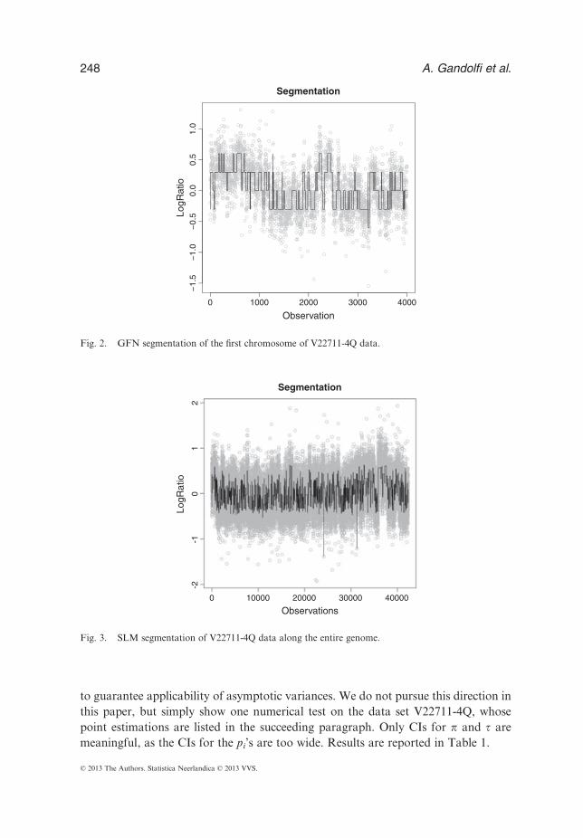
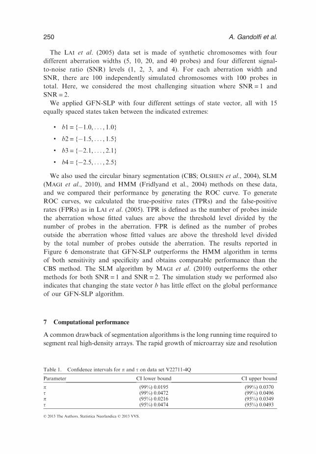
In particular, we can focus on the first chromosome, made of about 4000 clones, tosee better what happens in detail (Figure 2).The same data, analyzed with the SLM algorithm (see Magi et al. (2010)),
freely available on R environment, produce the segmentation shown in Figure 3;and highlighting the first chromosome as before, we obtain the segmentation inFigure 4.The second test has been performed on the genomic profile of chromosome 7 in
sample GBM29 of the BREDEL et al. (2005) data set; the results are plotted in Figure 5together with the SLM segmentation. Figure 5b shows that GFN-SLP is not able tocorrectly estimate the value of the state at the extremes. However, the principal aim ofa segmentation method is to predict the breakpoints of each segment. In fact, the fineestimation of the level of each state may be assessed by the usage of array-CGHcalling methods, such as FastCall (BENELLI et al., 2010) or CGHcall (VAN DE WIEL
et al., 2007).A comparison with other segmentations of the same data set appears in MAGI
et al. (2010).Numerical tests seem to indicate that our estimation method is quite sensitive, as
it identifies even small CNV regions, which are overlooked by other methods. Themain reason is the size of the estimated p, which is generally larger than othervalues usually adopted. Nonetheless, our method is able to identify large deletionsor amplifications.The asymptotic results of Theorem 2 allow, in principle, to write CIs for the
parameters. This is a relevant difference with other estimation methods, but itsapplication requires some accurate estimates on the sample size in order to be able
-2-1
01
2
0 10000 20000 30000 40000
Observations
LogR
atio
Segmentation
Fig. 1. GFN segmentation of V22711-4Q data along the entire genome.
GFN-SLP moment estimation 247
© 2013 The Authors. Statistica Neerlandica © 2013 VVS.
to guarantee applicability of asymptotic variances. We do not pursue this direction inthis paper, but simply show one numerical test on the data set V22711-4Q, whosepoint estimations are listed in the succeeding paragraph. Only CIs for p and t aremeaningful, as the CIs for the pi’s are too wide. Results are reported in Table 1.
-2-1
01
2
0 10000 20000 30000 40000
Observations
LogR
atio
Segmentation
Fig. 3. SLM segmentation of V22711-4Q data along the entire genome.
0 1000 2000 3000 4000
−1.
5−
1.0
−0.
50.
00.
51.
0
Segmentation
Observation
LogR
atio
Fig. 2. GFN segmentation of the first chromosome of V22711-4Q data.
248 A. Gandolfi et al.
© 2013 The Authors. Statistica Neerlandica © 2013 VVS.

6 Comparison with state-of-the-art algorithms
To estimate the accuracy of the GFN-SLP algorithm in identifying the aberrations atthe boundaries, we applied our algorithm on the synthetic chromosomes generated byLAI et al. (2005) (the data are freely available for download at http://www.chip.org/~ppark/Supplements/Bioinformatics05b.html).
0 50 100 150 200
−2
02
4
Segmentation
Observations
LogR
atio
(a) SLM segmentation
0 50 100 150 200
−2
02
4
Segmentation
Observations
LogR
atio
(b) GFN segmentation
Fig. 5. Comparison between the SLM and GFN segmentations on genomic profile of chromosome 7 insample GBM29 of BREDEL et al. (2005) data set.
0 1000 2000 3000 4000
−1.
5−
1.0
−0.
50.
00.
51.
0
Segmentation
Observation
LogR
atio
Fig. 4. SLM segmentation of the first chromosome of V22711-4Q data.
GFN-SLP moment estimation 249
© 2013 The Authors. Statistica Neerlandica © 2013 VVS.
The LAI et al. (2005) data set is made of synthetic chromosomes with fourdifferent aberration widths (5, 10, 20, and 40 probes) and four different signal-to-noise ratio (SNR) levels (1, 2, 3, and 4). For each aberration width andSNR, there are 100 independently simulated chromosomes with 100 probes intotal. Here, we considered the most challenging situation where SNR= 1 andSNR=2.We applied GFN-SLP with four different settings of state vector, all with 15
equally spaced states taken between the indicated extremes:
• b1= {�1.0, . . . , 1.0}
• b2= {�1.5, . . . , 1.5}
• b3= {�2.1, . . . , 2.1}
• b4= {�2.5, . . . , 2.5}
We also used the circular binary segmentation (CBS; OLSHEN et al., 2004), SLM(MAGI et al., 2010), and HMM (Fridlyand et al., 2004) methods on these data,and we compared their performance by generating the ROC curve. To generateROC curves, we calculated the true-positive rates (TPRs) and the false-positiverates (FPRs) as in LAI et al. (2005). TPR is defined as the number of probes insidethe aberration whose fitted values are above the threshold level divided by thenumber of probes in the aberration. FPR is defined as the number of probesoutside the aberration whose fitted values are above the threshold level dividedby the total number of probes outside the aberration. The results reported inFigure 6 demonstrate that GFN-SLP outperforms the HMM algorithm in termsof both sensitivity and specificity and obtains comparable performance than theCBS method. The SLM algorithm by MAGI et al. (2010) outperforms the othermethods for both SNR=1 and SNR=2. The simulation study we performed alsoindicates that changing the state vector b has little effect on the global performanceof our GFN-SLP algorithm.
7 Computational performance
A common drawback of segmentation algorithms is the long running time required tosegment real high-density arrays. The rapid growth of microarray size and resolution
Table 1. Confidence intervals for p and t on data set V22711-4Q
Parameter CI lower bound CI upper bound
p (99%) 0.0195 (99%) 0.0370t (99%) 0.0472 (99%) 0.0496p (95%) 0.0216 (95%) 0.0349t (95%) 0.0474 (95%) 0.0493
250 A. Gandolfi et al.
© 2013 The Authors. Statistica Neerlandica © 2013 VVS.

requires segmentation algorithms with high computational performance. For thisreason, we have tested the speed of GFN-SLP algorithm through an extensiveexperimentation on synthetic chromosomes and have compared its performance withrespect to that of the other three methods. To this end, we generated syntheticchromosomes with different numbers of alterations (from 1 to 10) and differentSNR (from 1 to 4).We have tested the computational performances of the three algorithms on
chromosomes with sizes from 500 to 32,000 clones (and with aberration width fixedto 30 clones).
0.0 0.2 0.4 0.6 0.8 1.0
0.0
0.2
0.4
0.6
0.8
1.0
FPR
TP
R
SNR=1
GFN b1GFN b2GFN b3GFN b4SLMCBSHMM
GFN b1 GFN b2 GFN b3 GFN b4 SLM CBS HMM
SNR=1
AU
C0.
00.
20.
40.
60.
8
0.72 0.73 0.72 0.7 0.85 0.72 0.63
0.0 0.2 0.4 0.6 0.8 1.0
0.0
0.2
0.4
0.6
0.8
1.0
FPR
TP
R
SNR=2
GFN b1GFN b2GFN b3GFN b4SLMCBSHMM
GFN b1 GFN b2 GFN b3 GFN b4 SLM CBS HMM
SNR=2
AU
C0.
00.
20.
40.
60.
8
0.93 0.93 0.92 0.92 0.96 0.92 0.9
Fig. 6. ROC curves and area under the curve bar plot for GFN, CBS, SLM, and HMM on the syntheticchromosomes of LAI et al. (2005) data set.
GFN-SLP moment estimation 251
© 2013 The Authors. Statistica Neerlandica © 2013 VVS.
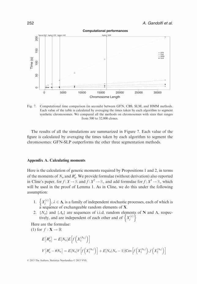
The results of all the simulations are summarized in Figure 7. Each value of thefigure is calculated by averaging the times taken by each algorithm to segment thechromosomes: GFN-SLP outperforms the other three segmentation methods.
Appendix A. Calculating moments
Here is the calculation of generic moments required by Propositions 1 and 2, in termsof the moments of Nn andRf
n. We provide formulae (without derivation) also reportedin Cline’s paper, for f :X!ℝ and f :X2!ℝ, and add formulae for f :X3!ℝ, whichwill be used in the proof of Lemma 1. As in Cline, we do this under the followingassumption:
1. X lð Þj
n o, l 2 Λ, is a family of independent stochastic processes, each of which is
a sequence of exchangeable random elements of X.2. {Nn} and {Λn} are sequences of i.i.d. random elements of N and Λ, respec-
tively, and are independent of each other and of X lð Þj
n oHere are the formulae:(1) for f : X ! R
E Rfn
� ¼ E Nn½ �E f X Λnð Þ1
� h i
V Rfn � θNn
� ¼ E Nn½ �V f X Λnð Þ1
� h iþ E Nn Nn � 1ð Þ½ �Cov f X Λnð Þ
1
� ; f X Λnð Þ
2
� h i
0 5000 10000 15000 20000 25000 30000
050
100
150
200
Computational performances
Chromosome Length
Tim
e (s
)
GFNCBSHMMSLM
Agilent 44KAgilent 22KTypical BAC Agilent 180K
Fig. 7. Computational time comparison (in seconds) between GFN, CBS, SLM, and HMM methods.Each value of the table is calculated by averaging the times taken by each algorithm to segmentsynthetic chromosomes. We compared all the methods on chromosomes with sizes that ranges
from 500 to 32,000 clones.
252 A. Gandolfi et al.
© 2013 The Authors. Statistica Neerlandica © 2013 VVS.

We observe that in this case the autocovariances between Rf�θi are all zero.
(2) for f : X2 ! R:
E Rfn
� ¼ E Nn � 1½ �E f X Λnð Þ1 ;X Λnð Þ
2
� h iþ E f X Λnð Þ
1 ;X Λnþ1ð Þ1
� h i:
V Rfn � θNn
� ¼ E Nn � 1½ �V f X Λnð Þ1 ;X Λnð Þ
2
� h iþ2E Nn � 2ð Þþ
�Cov f X Λnð Þ
1 ;X Λnð Þ2
� ; f X Λnð Þ
2 ;X Λnð Þ3
� h i
þE Nn � 2ð Þþ Nn � 3ð Þþ �
Cov f X Λnð Þ1 ;X Λnð Þ
2
� ; f X Λnð Þ
3 ;X Λnð Þ4
� h iþV f X Λnð Þ
1 ;X Λnþ1ð Þ1
� h iþ2P Nn > 1½ �Cov f X Λnð Þ
1 ;X Λnð Þ2
� ; f X Λnð Þ
2 ;X Λnþ1ð Þ1
� h i
þ2E Nn � 2ð Þþ �
Cov f X Λnð Þ1 ;X Λnð Þ
2
� ; f X Λnð Þ
3 ;X Λnþ1ð Þ1
� h i
þV Nn½ � E f X Λnð Þ1 ;X Λnð Þ
2
� � θ
h i� 2:
The autocovariances betweenRf�θi are all zero, except whenRf�θ
i are consecutiveelements of the process.
Cov Rf�θn ;Rf�θ
nþ1
h i¼ P Nnþ1 ¼ 1½ �Cov f X Λnð Þ
1 ;X Λnþ1ð Þ1
� ; f X Λnþ1ð Þ
1 ;X Λnþ2ð Þ1
� h i
þP Nnþ1 > 1½ �Cov f X Λnð Þ1 ;X Λnþ1ð Þ
1
� ; f X Λnþ1ð Þ
1 ;X Λnþ1ð Þ2
� h i
þE Nnþ1 � 2ð Þþ �
Cov f X Λnð Þ1 ;X Λnþ1ð Þ
1
� ; f X Λnþ1ð Þ
2 ;X Λnþ1ð Þ3
� h i
þP Nnþ1 > 1½ �Cov f X Λnð Þ1 ;X Λnþ1ð Þ
1
� ; f X Λnþ1ð Þ
2 ;X Λnþ2ð Þ1
� h i(3) for f : X3 ! R
E Rfn
� ¼ E Nn � 2ð Þþ �
E f X Λnð Þ1 ;X Λnð Þ
2 ;X Λnð Þ3
� h iþP Nn > 1½ �E f X Λnð Þ
1 ;X Λnð Þ2 ;X Λnþ1ð Þ
1
� h iþP Nnþ1 ¼ 1½ �E f X Λnð Þ
1 ;X Λnþ1ð Þ1 ;X Λnþ2ð Þ
1
� h iþP Nnþ1 > 1½ �E f X Λnð Þ
1 ;X Λnþ1ð Þ1 ;X Λnþ1ð Þ
2
� h i
GFN-SLP moment estimation 253
© 2013 The Authors. Statistica Neerlandica © 2013 VVS.

V Rf�θn
� ¼ E Nn � 2ð Þþ �
V f X Λnð Þ1 ;X Λnð Þ
2 ;X Λnð Þ3
� h i
þ2E Nn � 3ð Þþ �
Cov f X Λnð Þ1 ;X Λnð Þ
2 ;X Λnð Þ3
� ; f X Λnð Þ
2 ;X Λnð Þ3 ;X Λnð Þ
4
� h i
þ2E Nn � 4ð Þþ �
Cov f X Λnð Þ1 ;X Λnð Þ
2 ;X Λnð Þ3
� ; f X Λnð Þ
3 ;X Λnð Þ4 ;X Λnð Þ
5
� h i
þ2E Nn � 4ð Þþ �
E Nn � 5ð Þþ �
Cov f X Λnð Þ1 ;X Λnð Þ
2 ;X Λnð Þ3
� ; f X Λnð Þ
4 ;X Λnð Þ5 ;X Λnð Þ
6
� h i
þP Nn > 1½ �V f X Λnð Þ1 ;X Λnð Þ
2 ;X Λnþ1ð Þ1
� h i
þP Nnþ1 ¼ 1½ �V f X Λnð Þ1 ;X Λnþ1ð Þ
1 ;X Λnþ2ð Þ1
� h i
þP Nnþ1 > 1½ �V f X Λnð Þ1 ;X Λnþ1ð Þ
1 ;X Λnþ1ð Þ2
� h i
þ2P Nn > 2½ �Cov f X Λnð Þ1 ;X Λnð Þ
2 ;X Λnð Þ3
� ; f X Λnð Þ
2 ;X Λnð Þ3 ;X Λnþ1ð Þ
1
� h i
þ2P Nn > 3½ �Cov f X Λnð Þ1 ;X Λnð Þ
2 ;X Λnð Þ3
� ; f X Λnð Þ
3 ;X Λnð Þ4 ;X Λnþ1ð Þ
1
� h i
þ2E Nn � 4ð Þþ �
Cov f X Λnð Þ1 ;X Λnð Þ
2 ;X Λnð Þ3
� ; f X Λnð Þ
4 ;X Λnð Þ5 ;X Λnþ1ð Þ
1
� h i
þ2P Nnþ1 ¼ 1½ �P Nn > 2½ �Cov f X Λnð Þ1 ;X Λnð Þ
2 ;X Λnð Þ3
� ; f X Λnð Þ
3 ;X Λnþ1ð Þ1 ;X Λnþ2ð Þ
1
� h i
þ2P Nnþ1 ¼ 1½ �E Nn � 3ð Þþ �
Cov f X Λnð Þ1 ;X Λnð Þ
2 ;X Λnð Þ3
� ; f X Λnð Þ
4 ;X Λnþ1ð Þ1 ;X Λnþ2ð Þ
1
� h i
þ2P Nnþ1 > 1½ �P Nn > 2½ �Cov f X Λnð Þ1 ;X Λnð Þ
2 ;X Λnð Þ3
� ; f X Λnð Þ
3 ;X Λnþ1ð Þ1 ;X Λnþ1ð Þ
2
� h i
þ2P Nnþ1 > 1½ �E Nn � 3ð Þþ �
Cov f X Λnð Þ1 ;X Λnð Þ
2 ;X Λnð Þ3
� ; f X Λnð Þ
4 ;X Λnþ1ð Þ1 ;X Λnþ1ð Þ
2
� h i
þ2P Nnþ1 ¼ 1½ �P Nn > 1½ �Cov f X Λnð Þ1 ;X Λnð Þ
2 ;X Λnþ1ð Þ1
� ; f X Λnð Þ
2 ;X Λnþ1ð Þ1 ;X Λnþ2ð Þ
1
� h i
þ2P Nnþ1 > 1½ �P Nn > 1½ �Cov f X Λnð Þ1 ;X Λnð Þ
2 ;X Λnþ1ð Þ1
� ; f X Λnð Þ
2 ;X Λnþ1ð Þ1 ;X Λnþ1ð Þ
2
� h i
þV Nn½ � E f X Λnð Þ1 ;X Λnð Þ
2 ;X Λnð Þ3
� h i� θ
n o2
�2θP Nn ¼ 1½ �nE f X Λnð Þ
1 ;X Λnð Þ2 ;X Λnð Þ
3
� h i� E f X Λnð Þ
1 ;X Λnð Þ2 ;X Λnþ1ð Þ
1
� h ioþP Nn ¼ 1½ �P Nn > 1½ � E f X Λnð Þ
1 ;X Λnþ1ð Þ1 ;X Λnþ2ð Þ
1
� h i� E f X Λnð Þ
1 ;X Λnþ1ð Þ1 ;X Λnþ1ð Þ
2
� h i�n 2
� E f X Λnð Þ1 ;X Λnð Þ
2 ;X Λnð Þ3
� h i� E f X Λnð Þ
1 ;X Λnð Þ2 ;X Λnþ1ð Þ
1
� h i� 2oþ2P Nn ¼ 1½ � E f X Λnð Þ
1 ;X Λnð Þ2 ;X Λnð Þ
3
� h i� E f X Λnð Þ
1 ;X Λnð Þ2 ;X Λnþ1ð Þ
1
� h in o
� P Nn ¼ 1½ �E f X Λnð Þ1 ;X Λnþ1ð Þ
1 ;X Λnþ2ð Þ1
� h iþ P Nn > 1½ �E f X Λnð Þ
1 ;X Λnþ1ð Þ1 ;X Λnþ1ð Þ
2
� h in o:
In this case, there are two non-zero covariances:
254 A. Gandolfi et al.
© 2013 The Authors. Statistica Neerlandica © 2013 VVS.

Cov Rf�θn ;Rf�θ
nþ1
h i¼
¼ P Nn > 1½ �P Nnþ1 > 2½ �Cov f X Λnð Þ1 ;X Λnð Þ
2 ;X Λnþ1ð Þ1
� ; f X Λnþ1ð Þ
1 ;X Λnþ1ð Þ2 ;X Λnþ1ð Þ
3
� h iþ P Nn > 1½ �E Nn � 3ð Þþ
�Cov f X Λnð Þ
1 ;X Λnð Þ2 ;X Λnþ1ð Þ
1
� ; f X Λnþ1ð Þ
2 ;X Λnþ1ð Þ3 ;X Λnþ1ð Þ
4
� h i
þP Nn > 1½ �P Nnþ1 ¼ 2½ �Cov f X Λnð Þ1 ;X Λnð Þ
2 ;X Λnþ1ð Þ1
� ; f X Λnþ1ð Þ
1 ;X Λnþ1ð Þ2 ;X Λnþ2ð Þ
1
� h i
þP Nn > 1½ �P Nnþ1 > 2½ �Cov f X Λnð Þ1 ;X Λnð Þ
2 ;X Λnþ1ð Þ1
� ; f X Λnþ1ð Þ
2 ;X Λnþ1ð Þ3 ;X Λnþ2ð Þ
1
� h i
þP Nn > 1½ �P Nnþ1 ¼ 1½ �P Nnþ2 ¼ 1½ �Cov f X Λnð Þ1 ;X Λnð Þ
2 ;X Λnþ1ð Þ1
� ; f X Λnþ1ð Þ
1 ;X Λnþ2ð Þ1 ;X Λnþ3ð Þ
1
� h i
þP Nn > 1½ �P Nnþ1 > 1½ �P Nnþ2 ¼ 1½ �Cov f X Λnð Þ1 ;X Λnð Þ
2 ;X Λnþ1ð Þ1
� ; f X Λnþ1ð Þ
2 ;X Λnþ2ð Þ1 ;X Λnþ3ð Þ
1
� h iþP Nn > 1½ �P Nnþ1 ¼ 1½ �P Nnþ2 > 1½ �Cov f X Λnð Þ
1 ;X Λnð Þ2 ;X Λnþ1ð Þ
1
� ; f X Λnþ1ð Þ
1 ;X Λnþ2ð Þ1 ;X Λnþ2ð Þ
2
� h iþP Nn > 1½ �P Nnþ1 > 1½ �P Nnþ2 > 1½ �Cov f X Λnð Þ
1 ;X Λnð Þ2 ;X Λnþ1ð Þ
1
� ; f X Λnþ1ð Þ
2 ;X Λnþ2ð Þ1 ;X Λnþ2ð Þ
2
� h iþP Nnþ1 > 2½ �Cov f X Λnð Þ
1 ;X Λnþ1ð Þ1 ;X Λnþ1ð Þ
2
� ; f X Λnþ1ð Þ
1 ;X Λnþ1ð Þ2 ;X Λnþ1ð Þ
3
� h iþP Nnþ1 > 3½ �Cov f X Λnð Þ
1 ;X Λnþ1ð Þ1 ;X Λnþ1ð Þ
2
� ; f X Λnþ1ð Þ
2 ;X Λnþ1ð Þ3 ;X Λnþ1ð Þ
4
� h iþE Nn � 4ð Þþ �
Cov f X Λnð Þ1 ;X Λnþ1ð Þ
1 ;X Λnþ1ð Þ2
� ; f X Λnþ1ð Þ
3 ;X Λnþ1ð Þ4 ;X Λnþ1ð Þ
5
� h iþP Nnþ1 ¼ 2½ �Cov f X Λnð Þ
1 ;X Λnþ1ð Þ1 ;X Λnþ1ð Þ
2
� ; f X Λnþ1ð Þ
1 ;X Λnþ1ð Þ2 ;X Λnþ2ð Þ
1
� h iþP Nnþ1 ¼ 3½ �Cov f X Λnð Þ
1 ;X Λnþ1ð Þ1 ;X Λnþ1ð Þ
2
� ; f X Λnþ1ð Þ
2 ;X Λnþ1ð Þ3 ;X Λnþ2ð Þ
1
� h iþP Nnþ1 > 3½ �Cov f X Λnð Þ
1 ;X Λnþ1ð Þ1 ;X Λnþ1ð Þ
2
� ; f X Λnþ1ð Þ
3 ;X Λnþ1ð Þ4 ;X Λnþ2ð Þ
1
� h iþP Nnþ1 ¼ 1½ �P Nnþ2 ¼ 1½ �Cov f X Λnð Þ
1 ;X Λnþ1ð Þ1 ;X Λnþ2ð Þ
1
� ; f X Λnþ1ð Þ
1 ;X Λnþ2ð Þ1 ;X Λnþ3ð Þ
1
� h iþP Nnþ1 ¼ 2½ �P Nnþ2 ¼ 1½ �Cov f X1ð Λnð Þ;X Λnþ1ð Þ
1 ;X Λnþ1ð Þ2 ; f X Λnþ1ð Þ
2 ;X Λnþ2ð Þ1 ;X Λnþ3ð Þ
1
� h iþP Nnþ1 > 2½ �P Nnþ2 ¼ 1½ �Cov f X Λnð Þ
1 ;X Λnþ1ð Þ1 ;X Λnþ1ð Þ
2
� ; f X Λnþ1ð Þ
3 ;X Λnþ2ð Þ1 ;X Λnþ3ð Þ
1
� h iþP Nnþ1 ¼ 1½ �P Nnþ2 > 1½ �Cov f X Λnð Þ
1 ;X Λnþ1ð Þ1 ;X Λnþ2ð Þ
1
� ; f X Λnþ1ð Þ
1 ;X Λnþ2ð Þ1 ;X Λnþ2ð Þ
2
� h iþP Nnþ1 ¼ 2½ �P Nnþ2 > 1½ �Cov f X Λnð Þ
1 ;X Λnþ1ð Þ1 ;X Λnþ1ð Þ
2
� ; f X Λnþ1ð Þ
2 ;X Λnþ2ð Þ1 ;X Λnþ2ð Þ
2
� h iþP Nnþ1 > 2½ �P Nnþ2 > 1½ �Cov f X Λnð Þ
1 ;X Λnþ1ð Þ1 ;X Λnþ1ð Þ
2
� ; f X Λnþ1ð Þ
3 ;X Λnþ2ð Þ1 ;X Λnþ2ð Þ
2
� h iþθP Nn ¼ 1½ � E f X Λnð Þ
1 ;X Λnþ1ð Þ1 ;X Λnþ1ð Þ
2
� h i� E f X Λnð Þ
1 ;X Λnþ1ð Þ1 ;X Λnþ2ð Þ
1
� h in oþ P Nn ¼ 1½ �E f X Λnð Þ
1 ;X Λnþ1ð Þ1 ;X Λnþ2ð Þ
1
� h iþ P Nn > 1½ �E f X Λnð Þ
1 ;X Λnþ1ð Þ1 ;X Λnþ1ð Þ
2
� h in o2
�E f X Λnð Þ1 ;X Λnþ1ð Þ
1 ;X Λnþ1ð Þ2
� h i� P Nn ¼ 1½ �E f X Λnð Þ
1 ;X Λnþ1ð Þ1 ;X Λnþ2ð Þ
1
� h iþ P Nn > 1½ �E f X Λnð Þ
1 ;X Λnþ1ð Þ1 ;X Λnþ1ð Þ
2
� h in o
GFN-SLP moment estimation 255
© 2013 The Authors. Statistica Neerlandica © 2013 VVS.

Cov Rf�θn ;Rf�θ
nþ2
� ¼ P Nnþ1 ¼ 1½ �P Nnþ2 > 2½ �
�Cov f X Λnð Þ1 ;X Λnþ1ð Þ
1 ;X Λnþ2ð Þ1
� ; f X Λnþ2ð Þ
1 ;X Λnþ2ð Þ2 ;X Λnþ2ð Þ
3
� h iþ P Nnþ1 ¼ 1½ �E Nnþ2 � 3ð Þþ
��Cov f X Λnð Þ
1 ;X Λnþ1ð Þ1 ;X Λnþ2ð Þ
1
� ; f X Λnþ2ð Þ
2 ;X Λnþ2ð Þ3 ;X Λnþ2ð Þ
4
� h iþ P Nnþ1 ¼ 1½ �P Nnþ2 ¼ 2½ �
�Cov f X Λnð Þ1 ;X Λnþ1ð Þ
1 ;X Λnþ2ð Þ1
� ; f X Λnþ2ð Þ
1 ;X Λnþ2ð Þ2 ;X Λnþ3ð Þ
1
� h iþ P Nnþ1 ¼ 1½ �P Nnþ2 > 2½ �
�Cov f X Λnð Þ1 ;X Λnþ1ð Þ
1 ;X Λnþ2ð Þ1
� ; f X Λnþ2ð Þ
2 ;X Λnþ2ð Þ3 ;X Λnþ3ð Þ
1
� h iþP Nnþ1 ¼ 1½ �P Nnþ2 ¼ 1½ �P Nnþ3 ¼ 1½ �
�Cov f X Λnð Þ1 ;X Λnþ1ð Þ
1 ;X Λnþ2ð Þ1
� ; f X Λnþ2ð Þ
1 ;X Λnþ3ð Þ1 ;X Λnþ4ð Þ
1
� h iþP Nnþ1 ¼ 1½ �P Nnþ2 ¼ 1½ �P Nnþ3 > 1½ �
�Cov f X Λnð Þ1 ;X Λnþ1ð Þ
1 ;X Λnþ2ð Þ1
� ; f X Λnþ2ð Þ
1 ;X Λnþ3ð Þ1 ;X Λnþ3ð Þ
2
� h iþP Nnþ1 ¼ 1½ �P Nnþ2 > 1½ �P Nnþ3 ¼ 1½ �
�Cov f X Λnð Þ1 ;X Λnþ1ð Þ
1 ;X Λnþ2ð Þ1
� ; f X Λnþ2ð Þ
2 ;X Λnþ3ð Þ1 ;X Λnþ4ð Þ
1
� h iþP Nnþ1 ¼ 1½ �P Nnþ2 > 1½ �P Nnþ3 > 1½ �
�Cov f X Λnð Þ1 ;X Λnþ1ð Þ
1 ;X Λnþ2ð Þ1
� ; f X Λnþ2ð Þ
2 ;X Λnþ3ð Þ1 ;X Λnþ3ð Þ
2
� h i:
The preceding formulae can be used to compute the asymptotic variances g2f1 and g2f2
in Lemma 1; here is a sketchy derivation:
g2f1 ¼ w0 þ 2w1
¼ 1a1
V Rf1n � θf1Nn
�þ 2Cov Rf1n � θf1Nn;R
f1nþ1 � θf1Nnþ1
h in o
¼ 1a1
(a2 � 2a1 þ 1ð Þm4 þ 2a2 � 7a1 � 2pþ 6þ a2
a21
� �t4
þ 2a1 � a2 � 1þ a2a21
� �m2
2 þ 2 6a1 � 2a2 þ p� 4� a2a21
� �m2t2 þ a2
a21� 2
� �m4
1
þ2 a1 � 1ð Þm1m3 þ 2 2� a1 � a2a21
� �m2m
21 þ 2 �2a1 þ 2� pþ a2
a21
� �m2
1t2
þ2
"�m4
1 þ a1 � 1ð Þm1m3 þ 2� a1ð Þm2m21 þ 2 1� a1ð Þm2
1t2
#)
¼ 1a1
(a2 � 2a1 þ 1ð Þm4 þ 2a2 � 7a1 � 2pþ 6þ a2
a21
� �t4 þ 2a1 � a2 � 1þ a2
a21
� �m2
2
þ 12a1 � 4a2 þ 2p� 8� 2a2a21
� �m2t2 þ a2
a21� 4
� �m4
1 þ 4 a1 � 1ð Þm1m3
þ2 4� 2a1 � a2a21
� �m2m
21 � 2 4a1 þ p� 4� a2
a21
� �m2
1t2
);
256 A. Gandolfi et al.
© 2013 The Authors. Statistica Neerlandica © 2013 VVS.

g2f2 ¼ w0 þ 2w1 þ 2w2
¼ 1a1
V Rf2n � θf2Nn
�þ 2 Cov Rf2n � θf2Nn;R
f2nþ1 � θf2Nnþ1
h iþ 2Cov Rf2
n � θf2Nn;Rf2nþ2 � θf2Nnþ2
h in o
¼ 1a1
na2 � 4a1 þ 4� pð Þm4 þ
h2a2 � 11a1 � 2 p3 � 5p2 þ 9p� 8
� �þ 2p 2� pð Þ 1a1
þ 2� pð Þ2 a2a21
it4
þh4a1 � a2 þ 2p2 � 3p� 4þ 2p 2� pð Þ 1
a1þ 2� pð Þ2 a2
a21
im2
2
þh20a1 � 4a2 þ 2 p3 � 6p2 þ 12p� 12
� �� 4p 2� pð Þ 1a1
� 2 2� pð Þ2 a2a21
im2t2
þh4 p� 2ð Þ þ 2p 2� pð Þ 1
a1þ 2� pð Þ2 a2
a21
im4
1 þ 4 a1 þ p� 2ð Þm1m3
þh� 4a1 � 2 p� 2ð Þ pþ 4ð Þ � 4p 2� pð Þ 1
a1� 2 2� pð Þ2 a2
a21
im2m
21
þh� 8a1 þ 2 2� pð Þ p2 � 3pþ 3
� �þ 4p 2� pð Þ 1a1
þ 2 2� pð Þ2 a2a21
im2
1t2
þ2h� 4 1� pð Þm4
1 þ a1 2� pð Þ � 2� pð Þ2h i
m1m3 þ a1 p� 2ð Þ þ p2 � 8pþ 8 �
m2m21
þ2 a1 p� 2ð Þ þ p2 � 3pþ 3 �
m21t
2i
þ 2hp p� 2ð Þm4
1 þ ½pa1 þ p p� 2ð Þ�m1m3
þ �pa1 þ 2p 2� pð Þ½ �m2m21 þ �2pa1 þ p 3� pð Þ½ �m2
1t2io
¼ 1a1
na2 � 4a1 þ 4� pð Þm4 þ
þh2a2 � 11a1 � 2 p3 � 5p2 þ 9p� 8
� �þ 2� pð Þ2 a2a21
þ 2p 2� pð Þ 1a1
it4
þh4a1 � a2 þ 2p2 � 3p� 4þ 2p 2� pð Þ 1
a1þ 2� pð Þ2 a2
a21
im2
2
þ2h10a1 � 2a2 þ p3 � 6p2 þ 12p� 12� 2p 2� pð Þ 1
a1� 2� pð Þ2 a2
a21
im2t2
þh2 p2 þ 4p� 8� �þ 2p 2� pð Þ 1
a1þ 2� pð Þ2 a2
a21
im4
1 þ 8 a1 þ p� 2½ �m1m3
�2h4a1 þ 2 p2 þ 3p� 8
� �þ 2p 2� pð Þ 1a1
þ 2� pð Þ2 a2a21
im2m
21
�2h8a1 þ p3 � 6p2 þ 12p� 12� 2p 2� pð Þ 1
a1� 2� pð Þ2 a2
a21
im2
1t2o:
Finally, we compute the explicit expression of the off-diagonal terms ofC m1;m2;mf1 ;mf2ð Þ.
C m1;m2;mf1 ;mf2ð Þ 1; 2ð Þ ¼ C m1;m2;mf1 ;mf2ð Þ 2; 1ð Þ ¼ Cov m1; m2½ �¼ 1
a1Cov Rx
n � θxNn;Rx2n � θx2Nn
h i¼ 1
a1a2m3 � a2m1m2 þ 2m1t2 a1 � a2ð Þ� �
GFN-SLP moment estimation 257
© 2013 The Authors. Statistica Neerlandica © 2013 VVS.

C m1;m2;mf1 ;mf2ð Þ 1; 3ð Þ ¼ C m1;m2;mf1 ;mf2ð Þ 3; 1ð Þ ¼ Cov m1; mf1
�¼ 1
a1
nCov Rx
n � θxNn;Rf1n � θf1Nn
�þ Cov Rxnþ1 � θxNnþ1;R
f1n � θf1Nn
�o
¼ 1a1
nha2 � a1ð Þm3 � a1m3
1 þ 2a1 � a2ð Þm1m2
þ 3a1 � 2a2 � 1ð Þm1t2� þ ½�a1m31 þ a1m1m2 þ 1� a1ð Þm1t2
io¼ 1
a1
na2 � a1ð Þm3 � 2a1m3
1 þ 3a1 � a2ð Þm1m2 þ 2 a1 � a2ð Þm1t2o
C m1;m2;mf1 ;mf2ð Þ 2; 3ð Þ ¼ C m1;m2;mf1 ;mf2ð Þ 3; 2ð Þ ¼ Cov m2; mf1
� ¼ 1a1
nCov Rx2
n � θx2Nn;Rf1n � θf1Nn
h iþCov Rx2
nþ1 � θx2Nnþ1;Rf1n � θf1Nn
h io¼ 1
a1
nha2 � a1ð Þm4 þ 2 a2 � 3a1 þ 2ð Þt4 þ a1 � a2ð Þm2
2
þ4 2a1 � a2 � 1ð Þm2t2 þ a1m1m3 � a1m2m21 þ 2 1� a1ð Þm2
1t2i
þhaim1m3 � a1m2m
21 þ 2 1� a1ð Þm2
1t2io
¼ 1a1
na2 � a1ð Þm4 þ 2 a2 � 3a1 þ 2ð Þt4 þ a1 � a2ð Þm2
2
þ4 2a1 � a2 � 1ð Þm2t2 þ 2a1m1m3 � 2a1m2m21 þ 4 1� a1ð Þm2
1t2o
C m1;m2;mf1 ;mf2ð Þ 1; 4ð Þ ¼ C m1;m2;mf1 ;mf2ð Þ 4; 1ð Þ ¼ Cov m1; mf2
�¼ 1
a1
nCov Rx
n � θxNn;Rf2n � θf2Nn
�þ Cov Rxnþ1 � θxNnþ1;R
f2n � θf2Nn
�þCov Rx
nþ2 � θxNnþ2;Rf2n � θf2Nn
�o¼ 1
a1
nha2 � 2a1 þ pð Þm3 � 2a1 � pð Þm3
1 þ 4a1 � a2 � 2pð Þm1m2
þ2 2a1 � a2 � 1ð Þm1t2iþhpa1 � 2a1 þ pð Þm3
1
þ 2a1 � pa1 � pð Þm1m2 þ pa1 � 2a1 þ 2� pð Þm1t2i
þh� pa1m3
1 þ pa1m1m2 þ p 1� a1ð Þm1t2io
¼ 1a1
na2 � 2a1 þ pð Þm3 � 4a1 � 2pð Þm3
1 þ 6a1 � a2 � 3pð Þm1m2
þ2 a1 � a2ð Þm1t2o
C m1;m2;mf1 ;mf2ð Þ 2; 4ð Þ ¼ C m1;m2;mf1 ;mf2ð Þ 4; 2ð Þ ¼ Cov m2; mf2
�¼ 1
a1
nCov Rx2
n � θx2Nn;Rf2n � θf2Nn
h iþ Cov Rx2
nþ1 � θx2Nnþ1;Rf2n � θf2Nn
h iþCov Rx2
nþ2 � θx2Nnþ2;Rf2n � θf2Nn
h io¼ 1
a1
nha2 � 2a1 þ pð Þm4 þ 2 a2 � 4a1 � pþ 4ð Þt4 þ 2a1 � a2 � pð Þm2
2
þ4 3a1 � a2 � 2ð Þm2t2 þ 2a1 � pð Þm1m3 þ p� 2a1ð Þm2m21
þ4 1� a1ð Þm21t
2iþh2a1 � pa1 � pð Þm1m3 þ pa1 � 2a1 þ pð Þm2m
21
þ2 pa1 � 2a1 � pþ 2ð Þm21t
2i
þhpa1m1m3 � pa1m2m
21 þ 2p 1� a1ð Þm2
1t2io
¼ 1a1
na2 � 2a1 þ pð Þm4 þ 2 a2 � 4a1 � pþ 4ð Þt4 þ 2a1 � a2 � pð Þm2
2
þ4 3a1 � a2 � 2ð Þm2t2 þ 2 2a1 � pð Þm1m3 þ 2 p� 2a1ð Þm2m21
þ8 1� a1ð Þm21t
2o
258 A. Gandolfi et al.
© 2013 The Authors. Statistica Neerlandica © 2013 VVS.
C m1;m2;mf1 ;mf2ð Þ 3; 4ð Þ ¼ C m1;m2;mf1 ;mf2ð Þ 4; 3ð Þ ¼ Cov mf1 ; mf2
�
¼ 1a1
(Cov Rf1
n � θf1Nn;Rf2n � θf2Nn
�þ Cov Rf1nþ1 � θf1Nnþ1;R
f2n � θf2Nn
h i
þCov Rf1nþ2 � θf1Nnþ2;R
f2n � θf2Nn
h i
þCov Rf1n�1 � θf1Nn�1;R
f2n � θf2Nn
h i)
¼ 1a1
nha2 � 3a1 þ 2ð Þm4
þ 2a2 � 10a1 þ 2p2 � 8pþ 12þ p1a1
þ 2� pð Þ a2a21
� �t4
þ 3a1 � a2 � 2p� 2þ p1a1
þ 2� pð Þ a2a21
� �m2
2
þ2 8a1 � 2a2 � p2 þ 5p� 8� p1a1
� 2� pð Þ a2a21
� �m2t2
þ p� 4þ p1a1
þ 2� pð Þ a2a21
� �m4
1 þ 3a1 þ p� 4ð Þm1m3
þ 8� 3a1 � 2p1a1
þ 2 p� 2ð Þ a2a21
� �m2m
21
þ2 �3a1 þ p2 � 4pþ 4þ p1a1
þ 2� pð Þ a2a21
� �m2
1t2i
þhp� 2ð Þm4
1 þ a1 � 1ð Þ 2� pð Þm1m3 þ 2� pð Þ 2� a1ð Þm2m21
þ 2a1 p� 2ð Þ þ 5� 3p½ �m21t
2i
þh� pm4
1 þ p a1 � 1ð Þm1m3 þ p 2� a1ð Þm2m21 þ 2p 1� a1ð Þm2
1t2i
þhp� 2ð Þm4
1 þ a1 þ p� 2ð Þm1m3 � a1 þ 2p� 4ð Þm2m21
þ �2a1 � pþ 3ð Þm21t
2io
¼ 1a1
(a2 � 3a1 þ 2ð Þm4
þ 2a2 � 10a1 þ 2p2 � 8pþ 12þ p1a1
þ 2� pð Þ a2a21
�t4
þ 3a1 � a2 � 2p� 2þ p1a1
þ 2� pð Þ a2a21
�m2
2
þ2 8a1 � 2a2 � p2 þ 5p� 8� p1a1
� 2� pð Þ a2a21
�m2t2
þ 2p� 8þ p1a1
þ 2� pð Þ a2a21
�m4
1
þ2 3a1 þ p� 4ð Þm1m3 � 2 3a1 þ p� 8þ p1a1
þ 2� pð Þ a2a21
�m2m
21
þ2 �6a1 þ p2 � 5pþ 8þ p1a1
þ 2� pð Þ a2a21
�m2
1t2
):
GFN-SLP moment estimation 259
© 2013 The Authors. Statistica Neerlandica © 2013 VVS.

Appendix B. Correcting Cline’s error
CLINE’s paper (1983) assumes normality of the level distribution and thus derivesformulae under that assumption. Such formulae can be derived by those computedhere, in particular from those expressed only in terms of p, which appears also inCLINE (1983), t, appearing in CLINE (1983) with a different parametrization, andmi’s, which are the moments of the level distribution and can thus be derived in termsof Cline’s parameters. The needed parameter change is thus
p ¼ pt2 ¼ 1� rð Þs2
m1 ¼ m1 ¼ mm2 ¼ m2 þ t2 ¼ m2 þ s2
m3 ¼ m3 þ 3m1t2 ¼ m3 þ 3ms2
m4 ¼ m4 þ 6m2t2 þ 3t4 ¼ m4 þ 6m2s2 þ 3s4:
We thus checked all of Cline’s expressions, finding two errors, which we report tomake Cline’s formulae directly usable.The first error concernsCov Rx
n � θxNn;Rf1n � θf1Nn
�, and it is simply a typo because
the subsequent formulae use the correct expression:
Cov Rxn � θxNn;Rf1
n � θf1Nn
� ¼ a2 � a1ð Þm3 � a1m31 þ 2a1 � a2ð Þm1m2
þ 3a1 � 2a2 � 1ð Þm1t2
¼ 1p
2� pð Þ þ r1� pð Þ 4� pð Þ
p
�ms2
where the first equality follows from the GFN model , whereas the second is the onewith GNN parameters.Instead, the second error is not directly comparable with one of our asymptotic
value as it appears in calculation of asymptotic distribution of the secondautocovariances present in Cline but not in our model. However, it can be retrievedby calculating the asymptotic variance of the autocovariance g2, as it is denoted inCline paper, through a multidimensional delta method characterized by the followingelements: the function
g2 : R2 ! Rm1; mf2
� �↦ g2 ¼ mf2 � m2
1
whose gradient is rg2 m1; ;mf2
� � ¼ �2m1; 1ð Þ and the variance–covariance matrix
C m1;;mf2ð Þ ¼g21 Cov m1; ; mf2
�Cov m1; ; mf2
�g2f2
�:
where all elements are already known. Then it follows that
260 A. Gandolfi et al.
© 2013 The Authors. Statistica Neerlandica © 2013 VVS.

V g2½ � ¼ 1nrg2C m1;;mf2ð Þrgt2 ¼
s4
n1þ 1� pð Þ4 2r� 5r2
� �þ 41� pð Þ2
pr2
" #
where the second equality is obtained by replacing the GFN-SLM parameters withthe GNN-SLM ones.We finally verify that the formula in CLINE (1983) is incorrect. This can be easily
observed in the case p=1; this is a perfectly acceptable range of parameters for theGNN-SLM model, whereas our derivation, albeit carried out on the assumption thatp< 1, does not actually depend on that assumption for V[g1] and V[g2]. In such case,the Xi’s are independent, and thus, there should be no difference between the twoautocovariances defined by Cline, g1 and g2. As a consequence, the asymptotic distri-butions of g1 and g2 should be the same, and in particular, the two asymptotic vari-ances should be the same, that is, V[g1] =V[g2]. We report in the following the twoexpressions as they appear in Cline:
V g1½ � ¼ s4
n1þ 2r� 3r2
� �1� pð Þ2 þ 2 1� pð Þ 2� pð Þ
pr2
�
V g2½ � ¼ s4
n1þ 2r� 5r2
� �1� pð Þ4 þ 2r2
1� pð Þ2 þ 2� pð Þ2 � 1� pð Þ4p 2� pð Þ
" #( )
If we evaluate the latter expression for p=1, we obtain thatV g2½ � ¼ 1þ 2r2ð Þs4n , in-stead of the value V g1½ � ¼ s4
n , which coincides with that of the variance V[g2] that wehave calculated earlier.
REFERENCES
BAYANI, J., S. SELVARAJAH, G. MAIRE, B. VUKOVIC, K. AL-ROMAIH, M. ZIELENSKA andJ. A. SQUIRE (2007), Genomic mechanisms and measurement of structural and numericalinstability in cancer cells, Seminars in Cancer Biology 17, 5–18
BENELLI, M., G. MARSEGLIA, G. NANNETTI, R. PARAVIDINO, F. ZARA, F. D. BRICARELLI,F. TORRICELLI and A. MAGI (2010), A very fast and accurate method for calling aberrationsin array-CGH data, Biostatistics 11, 515–518
BREDEL, M., C. BREDEL, D. JURIC, G. R. HARSH, H. VOGEL, L. D. RECHT and B. I. SIKIC(2005), High-resolution genomic-wide mapping of genetic alterations in human glial braintumors, Cancer Research 65, 4088–4096.
CARTER N. P. (2007), Methods and strategies for analyzing copy number variation using DNAmicroarrays, Nature Genetics 39, S16–S21.
CHERNOFF, H. and S. ZACKS (1964), Estimating the current mean of a normal distributionwhich is subjected to change in time. The Annals of Mathematical Statistics 35, 999–1018.
CLINE, D. B. H. (1983), Limit theorems for the shifting level process, Journal of Appliedprobability 20, 322–337.
FORNEY, G. D. (1973), The Viterbi algorithm, Proceedings of the IEEE 61, 268–278.FORTIN, V. and A. KEHAGIAS (2006), Time series segmentation with shifting means hiddenMarkov models. Nonlinear Processes in Geophysics 13, 135–163.
FRIDLYAND, J., A. M. SNIJDERS, D. PINKEL, D. G. A. ALBERTSON and A. N. JAIN (2004),HiddenMarkov models approach to the analysis of array-CGH data, Journal of MultivariateAnalysis 90, 132–153.
GFN-SLP moment estimation 261
© 2013 The Authors. Statistica Neerlandica © 2013 VVS.

HUPE P., N. STRANSKY, J. P. THIERY, F. RADVANYI and E. BARILLOT (2004), Analysis ofarray CGH data: from signal ratio to gain and loss of DNA regions, Bioinformatics 20,3413–3422.
LAI, W. R. R., M. D. D. JOHNSON, R. KUCHERLAPATI and P. J. J. PARK (2005), Compara-tive analysis of algorithms for identifying amplifications and deletions in array-CGH data,Bioinformatics 21, 3763–3770.
LEPRETRE, F., C. VILLENET, S. QUIEF, O. NIBOUREL, C. JACQUEMIN, X. TROUSSARD,F. JARDIN, F. GIBSON, J. P. KERCKAERT, C. ROUMIER and M. FIGEAC (2010), WavedaCGH: to smooth or not to smooth, Nucleic Acids Research 38, e94.
LIU, X. S. (2007), Getting started in tiling microarray analysis, PLoS Computational Biology3, e183, 1842–1844.
MAGI, A., M. BENELLI, G. MARSEGLIA, G. NANNETTI, M. R. SCORDO and F. TORRICELLI(2010), A shifting level model algorithm that identifies aberrations in array-CGH data.Biostatistics 11(2), 265.
MYERS C. L., M. J. DUNHAM, S. Y. KUNG and O. G. TROYANSKAYA (2004), Accurate detec-tion of aneuploidies in array CGH and gene expression microarray data, Bioinformatics 20,3533–3543.
OLSHEN, A. B., E. S. VENKATRAMAN, R. LUCITO and M. WIGLER (2004), Circularbinary segmentation for the analysis of array-based DNA copy number data, Biostatistics5, 557–72.
OOSTLANDER, A. E., G. A. MEIJER and B. YLSTRA (2004), Microarray-based comparativegenomic hybridization and its applications in human genetics, Clinical Genetics 66, 488–495.
PICARD, F., S. ROBIN, M. LAVIELLE, C. VAISSE and J.-J. DAUDIN (2005), A statisticalapproach for array CGH data analysis, BMC Bioinformatics 6, 1–14.
SALAS, J. D. and D. C. BOES (1980), Shifting level modelling of hydrologic time series,Advances in Water Resources 3, 59–63.
VAN DE WIEL, M., I. K. KIM, S. J. VOSSE, W. N. VAN WIERINGEN, S. M. WILTING andB. YLSTRA (2007), CGHcall: calling aberrations for array CGH tumor profiles, Bioinformatics7, 892–894.
YOON, S., Z. XUAN, V. MAKAROV, K. YE and J. SEBAT (2009), Sensitive and accurate detec-tion of copy number variants using read depth of coverage, Genome Research 19, 1586–1592.
Received: 30 January 2011. Revised: 31 January 2013.
262 A. Gandolfi et al.
© 2013 The Authors. Statistica Neerlandica © 2013 VVS.
Related Documents