Does Proximity Matter? Distance Dependence of Adolescent Friendships

Page 1

D

Pa

b

c

d

a

KANGD

1

tt1ecicgcaM

s

Th

0d

Social Networks 34 (2012) 18– 31

Contents lists available at ScienceDirect

Social Networks

jo ur nal homep ag e: www.elsev ier .com/ locate /socnet

oes proximity matter? Distance dependence of adolescent friendships

aulina Preciadoa,∗, Tom A.B. Snijdersb, William J. Burkc, Håkan Stattind, Margaret Kerrd

University of Oxford, Department of Statistics, 1 South Parks Road, Oxford OX1 3TG, United KingdomUniversity of Oxford and University of Groningen, Nuffield College, New Road, Oxford OX1 1NF, United KingdomRadboud Universiteit Nijmegen, Montessorilaan 3, 6525 HR Nijmegen, The NetherlandsUniversity of Örebro, Fakultetsgatan 1, 701 82 Örebro, Sweden

r t i c l e i n f o

eywords:dolescent friendshipetwork dynamicseographic proximityistance

a b s t r a c t

Geographic proximity is a determinant factor of friendship. Friendship datasets that include detailedgeographic information are scarce, and when this information is available, the dependence of friendshipon distance is often modelled by pre-specified parametric functions or derived from theory withoutfurther empirical assessment. This paper aims to give a detailed representation of the association betweendistance and the likelihood of friendship existence and friendship dynamics, and how this is modified bya few basic social and individual factors. The data employed is a three-wave network of 336 adolescentsliving in a small Swedish town, for whom information has been collected on their household locations.The analysis is a three-step process that combines (1) nonparametric logistic regressions to unravel theoverall functional form of the dependence of friendship on distance, without assuming it has a particularstrength or shape; (2) parametric logistic regressions to construct suitable transformations of distancethat can be employed in (3) stochastic models for longitudinal network data, to assess how distance,

individual covariates, and network structure shape adolescent friendship dynamics. It was found thatthe log-odds of friendship existence and friendship dynamics decrease smoothly with the logarithm ofdistance. For adolescents in different schools the dependence is linear, and stronger than for adolescentsin the same school. Living nearby accounts, in this dataset, for an aspect of friendship dynamics thatis not explicitly modelled by network structure or by individual covariates. In particular, the estimateddistance effect is not correlated with reciprocity or transitivity effects.

. Introduction

Homophily is a major characteristic of friendship: individualsend to become and remain friends with others that are similaro them (e.g., Lazarsfeld and Merton, 1954; Cohen, 1997; Kandel,978; McPherson et al., 2001). Geographic proximity is one of thessential causes of homophily because people that are spatiallylose are more likely to meet and interact, and because geograph-cally bounded organizations, such as neighbourhoods or schools,ongregate individuals who are similar in characteristics like reli-ion, ethnicity, income, etc. Hence, spatial propinquity fosters thereation and maintenance of relationships between people thatre alike (Lieberson, 1980; Feld, 1982; Blau and Schwartz, 1984;

cPherson et al., 2001).The literature argues that the probability, contact frequency, and

trength of social ties decline with distance. Wellman (1996) found

∗ Corresponding author. Tel.: +44 1865272860.E-mail addresses: [email protected] (P. Preciado),

[email protected] (T.A.B. Snijders), [email protected] (W.J. Burk),[email protected] (H. Stattin), [email protected] (M. Kerr).

378-8733/$ – see front matter © 2011 Elsevier B.V. All rights reserved.oi:10.1016/j.socnet.2011.01.002

© 2011 Elsevier B.V. All rights reserved.

that most types of relationships, especially those characterised byfrequent interactions, occur more often within one mile of an indi-vidual’s home than farther away. In agreement, Carrasco et al.(2008) state that after accounting for gender, age, income, use ofcommunication technologies and degree of closeness in a relation-ship, individuals have to be more proactive in seeking opportunitiesfor socialising with those who live more than 35 km away than withthose living closer by.

Moreover, the development of modern transportation and com-munication technologies has not destroyed, but transformed anddiversified, the effect that geographic proximity has on socialrelations (Dijst, 2006). Real friendships grow through tangibleinteractions, which are less expensive at shorter distances (Butts,2002). Residential proximity is amongst the strongest predictorsof how often friends get together to socialise (Verbrugge, 1983;Tsai, 2006), and relationships solely based on non face-to-face con-tacts (such as e-mail or telephone) usually originate and developon pre-existing, tangible ties (Carley and Wendt, 1991).

While the general agreement is that the likelihood of social rela-tionships decreases with distance, little is known about the relevantfeatures of this falloff and how it changes in time and by other spa-tial and social factors. This is partially because longitudinal network

Page 2

l Netw

d(mt

tHstRvc

geBftmio(f

amapau

dmFmsairyia

Swrs

idmb

wtfiasl

wie

P. Preciado et al. / Socia

ata that includes the exact location of the actors is rather scarceparticularly if the actors are human individuals), and also because

ost network studies are spatially constrained, so geographic dis-ances might not play a major role (Butts, 2002).

Many social institutions are organised in space, implying thatheir effects on relationships might be correlated with distance.ence, accounting for spatial arrangements and distances amongst

ocial actors is important when analysing social processes, insti-utions and contexts, as argued by White (1992) and Pattison andobins (2002). When the distance dependence of friendship is rele-ant, a misspecification of its functional form may lead to erroneousonclusions about other, spatially bounded social factors.

Some relevant studies have focused on the influence of geo-raphic proximity on social relationships in more detail, usuallymploying an exponential or a power-law (e.g. Latané et al., 1995;utts, 2002; Liben-Nowell et al., 2005; Daraganova et al., submitted

or publication). In particular, Latané et al. (1995) conclude thathe average number of interactions people find noteworthy or

emorable, is proportional to the inverse of the distance at whichndividuals live, and argue that this is in accordance with the the-ry of social impact (Latané, 1981), which states that social impactin the form of spending time with, being influenced by, etc.) is aunction of the inverse square of distance.1

In many of these works, however, the functional form of thessociation between distance and social relationships is eitherodelled by pre-specified parametric functions, or by rough

pproximations. Further, they often assume that the ties betweenairs of actors are independent, so even when pertinent individualnd social characteristics are accounted for, network structure issually not considered.

This paper aims to give a detailed representation of the depen-ence of friendship on distance, and how this dependence isodified by a few basic individual characteristics and social factors.

irst, we find the functional form of the effect of distance withoutaking any assumptions about its relevant features. Next, we con-

truct parametric estimates of this effect to assess how its strengthnd shape change in time and in the presence of basic similarity andnstitutional proximity measurements. Finally, we employ theseesults in parametric models for longitudinal social network anal-sis, to study how the association between friendship and distances modified when the interdependent nature of the relationships,nd the structural characteristics of a network are considered.

We employ an age-defined cohort of adolescents living in a smallwedish town for whom there is information on the distance athich they live. The study design is such (see Section 3), that it is

easonable to assume the dataset represents practically all friend-hips with frequent contacts for adolescents of this age in the town.

The first aim of this article is data-analytic and methodologicaln nature. A second aim is to get substantive insights about theistance dependence of adolescent friendship. In this respect theodel tests a number of hypotheses, indicated by H1–H5 below,

ased on the following theoretical considerations and expectations.In general, we expect for the likelihood of friendship to decrease

ith distance (H1), because proximity between households leadso increasing opportunities, and decreasing costs of various kinds,or meeting and interaction (Zipf, 1949; Verbrugge, 1983). Attend-ng the same school also yields meeting opportunities, with the

dded component that in school the adolescents are together for aignificant part of the day, which is not necessarily the case if theyive close by. Schools as well as neighbourhoods (short distances)

1 It is assumed that people are evenly distributed in space, so the number of peopleho live at a certain distance r from the centre (where the focal actor lives), increases

n proportion to this radius. Hence, if social impact is proportional to 1/r2 then thexpected number of memorable social interactions should be proportional to 1/r.

orks 34 (2012) 18– 31 19

yield foci for social contacts (Feld, 1981). Hence, we hypothesizethat the effect of living nearby on the likelihood of friendship willbe weaker if the adolescents go to the same schools (H2). Also, asadolescents grow older they become less dependent on their par-ents (Steinberg and Silveberg, 1986) and will have more resourcesto explore spaces further away from home, so the distance depen-dence of friendships should become weaker as they age (H3). Inaddition, we expect that estimated effects of distance on friendshipwill become weaker when tendencies towards transitivity and reci-procity (which may be expected to be important, cf., e.g., Hallinan,1974) are considered, because their effects might be correlated(H4). Finally, we expect the dependence of friendship creation ondistance to be stronger than that of friendship maintenance (H5), asin the latter the distance-related cost or effort necessary to establisha friendship has already been overcome (Zipf, 1949).

This study can hopefully serve a dual purpose. On the one hand,the results, although based on a data set from one town, may havesome degree of generalisability to other places and can thus pro-vide insight in the ways in which a meaningful geographic contextinfluences friendships between adolescents. On the other hand, themethodological approach may serve as a point of departure forother studies of distance dependence.

2. Methodology

We consider longitudinal social network data that consists ofrepeated observations of a set of n actors (or nodes) and therelationships between them (or ties), along with the geographiclocation of the actors and other individual or pairwise attributes.Ties are regarded as binary (i.e., existent or non-existent) and it isassumed that the locations of the actors are constant in time.

To assess the effect of geographic proximity on the probabilityof friendship we would ideally employ a fully flexible model fordistance together with network dependence; but a method com-bining these in a single analysis is yet unavailable. Therefore, wefollow a three-step process. First, using logistic Generalized Addi-tive Models (“GAM”; Hastie and Tibshirani, 1986), a descriptiveapproach is elaborated in which the network dependence is ignoredand the n(n − 1) binary tie variables are treated as if they wereindependent, but allowing complete generality in the functionalform. This yields a detailed description of the relevant featuresof the effect of spatial distance on friendship. Second, the effectsobtained are approximated by parsimonious parametric functions,using standard logistic regressions. This produces a small numberof transformations of distance for which a linear combination givesa close representation of the effect of distance on the log-oddsof friendship, under the assumption of tie independence. We dothis in both a static (existence of friendships) and a dynamic (cre-ation and maintenance of friendships) perspective. Finally, thesetransformations of distance are used in Stochastic Actor-OrientedModels (“SAOM”; Snijders, 2001) for network dynamics, a para-metric framework that allows analysing the distance effect onfriendship while fully taking into account network dependencies.The third step is carried out only for the dynamic case, because thenumber of analyses presented is already quite large, and becausethe static instance is covered by Daraganova et al. (submitted forpublication).

2.1. Generalized Additive Models

Generalized Additive Models were formulated by Hastie and

Tibshirani (1986) as an extension to Generalized Linear Mod-els (GLM) that allow the inclusion of smooth functions of theexplanatory variables along with the standard parametric compo-nents. They are particularly useful when the functional form of the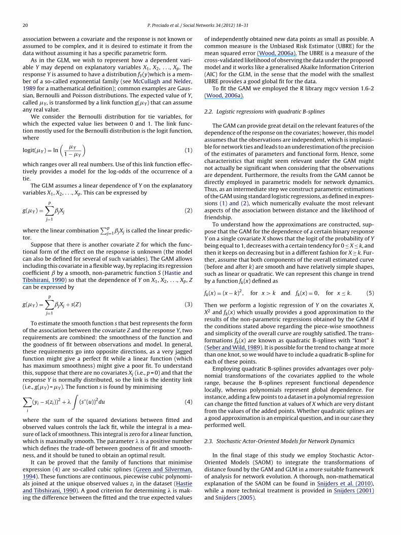

Page 3

2 l Netw

aad

arb1sca

wtw

l

wtt

v

g

wt

tcicTc

g

orttfhtr(

∑

woswwn

e1aai

0 P. Preciado et al. / Socia

ssociation between a covariate and the response is not known orssumed to be complex, and it is desired to estimate it from theata without assuming it has a specific parametric form.

As in the GLM, we wish to represent how a dependent vari-ble Y may depend on explanatory variables X1, X2, . . ., Xp. Theesponse Y is assumed to have a distribution fY(y)which is a mem-er of a so-called exponential family (see McCullagh and Nelder,989 for a mathematical definition); common examples are Gaus-ian, Bernoulli and Poisson distributions. The expected value of Y,alled �Y, is transformed by a link function g(�Y) that can assumeny real value.

We consider the Bernoulli distribution for tie variables, forhich the expected value lies between 0 and 1. The link func-

ion mostly used for the Bernoulli distribution is the logit function,here

ogit(�Y ) = ln(

�Y

1 − �Y

)(1)

hich ranges over all real numbers. Use of this link function effec-ively provides a model for the log-odds of the occurrence of aie.

The GLM assumes a linear dependence of Y on the explanatoryariables X1, X2, . . ., Xp. This can be expressed by

(�Y ) =p∑

j=1

ˇjXj (2)

here the linear combination∑p

j=1ˇjXj is called the linear predic-or.

Suppose that there is another covariate Z for which the func-ional form of the effect on the response is unknown (the modelan also be defined for several of such variables). The GAM allowsncluding this covariate in a flexible way, by replacing its regressionoefficient by a smooth, non-parametric function S (Hastie andibshirani, 1990) so that the dependence of Y on X1, X2, . . ., Xp, Zan be expressed by

(�Y ) =p∑

j=1

ˇjXj + s(Z) (3)

To estimate the smooth function s that best represents the formf the association between the covariate Z and the response Y, twoequirements are combined: the smoothness of the function andhe goodness of fit between observations and model. In general,hese requirements go into opposite directions, as a very jaggedunction might give a perfect fit while a linear function (whichas maximum smoothness) might give a poor fit. To understandhis, suppose that there are no covariates Xj (i.e., p = 0) and that theesponse Y is normally distributed, so the link is the identity linki.e., g(�Y) = �Y). The function s is found by minimising

i

(yi − s(zi))2 + �

∫(s′′(u))2du (4)

here the sum of the squared deviations between fitted andbserved values controls the lack fit, while the integral is a mea-ure of lack of smoothness. This integral is zero for a linear function,hich is maximally smooth. The parameter � is a positive numberhich defines the trade-off between goodness of fit and smooth-ess, and it should be tuned to obtain an optimal result.

It can be proved that the family of functions that minimisexpression (4) are so-called cubic splines (Green and Silverman,

994). These functions are continuous, piecewise cubic polynomi-ls joined at the unique observed values zi in the dataset (Hastiend Tibshirani, 1990). A good criterion for determining � is mak-ng the difference between the fitted and the true expected values

orks 34 (2012) 18– 31

of independently obtained new data points as small as possible. Acommon measure is the Unbiased Risk Estimator (UBRE) for themean squared error (Wood, 2006a). The UBRE is a measure of thecross-validated likelihood of observing the data under the proposedmodel and it works like a generalised Akaike Information Criterion(AIC) for the GLM, in the sense that the model with the smallestUBRE provides a good global fit for the data.

To fit the GAM we employed the R library mgcv version 1.6-2(Wood, 2006a).

2.2. Logistic regressions with quadratic B-splines

The GAM can provide great detail on the relevant features of thedependence of the response on the covariates; however, this modelassumes that the observations are independent, which is implausi-ble for network ties and leads to an underestimation of the precisionof the estimates of parameters and functional form. Hence, somecharacteristics that might seem relevant under the GAM mightnot actually be significant when considering that the observationsare dependent. Furthermore, the results from the GAM cannot bedirectly employed in parametric models for network dynamics.Thus, as an intermediate step we construct parametric estimationsof the GAM using standard logistic regressions, as defined in expres-sions (1) and (2), which numerically evaluate the most relevantaspects of the association between distance and the likelihood offriendship.

To understand how the approximations are constructed, sup-pose that the GAM for the dependence of a certain binary responseY on a single covariate X shows that the logit of the probability of Ybeing equal to 1, decreases with a certain tendency for 0 ≤ X ≤ k, andthen it keeps on decreasing but in a different fashion for X ≥ k. Fur-ther, assume that both components of the overall estimated curve(before and after k) are smooth and have relatively simple shapes,such as linear or quadratic. We can represent this change in trendby a function fk(x) defined as

fk(x) = (x − k)2, for x > k and fk(x) = 0, for x ≤ k. (5)

Then we perform a logistic regression of Y on the covariates X,X2 and fk(x) which usually provides a good approximation to theresults of the non-parametric regressions obtained by the GAM ifthe conditions stated above regarding the piece-wise smoothnessand simplicity of the overall curve are roughly satisfied. The trans-formations fk(x) are known as quadratic B-splines with “knot” k(Seber and Wild, 1989). It is possible for the trend to change at morethan one knot, so we would have to include a quadratic B-spline foreach of these points.

Employing quadratic B-splines provides advantages over poly-nomial transformations of the covariates applied to the wholerange, because the B-splines represent functional dependencelocally, whereas polynomials represent global dependence. Forinstance, adding a few points to a dataset in a polynomial regressioncan change the fitted function at values of X which are very distantfrom the values of the added points. Whether quadratic splines area good approximation is an empirical question, and in our case theyperformed well.

2.3. Stochastic Actor-Oriented Models for Network Dynamics

In the final stage of this study we employ Stochastic Actor-Oriented Models (SAOM) to integrate the transformations ofdistance found by the GAM and GLM in a more suitable framework

of analysis for network evolution. A thorough, non-mathematicalexplanation of the SAOM can be found in Snijders et al. (2010),while a more technical treatment is provided in Snijders (2001)and Snijders (2005).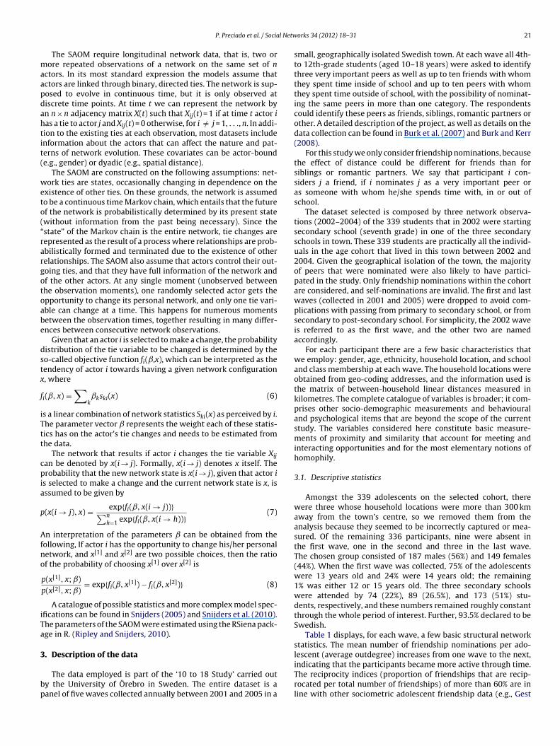

Page 4

l Netw

maapdahtit(

weto(“rargotoabe

dstx

f

iTtt

cpia

p

Afno

iTa

3

bp

P. Preciado et al. / Socia

The SAOM require longitudinal network data, that is, two orore repeated observations of a network on the same set of n

ctors. In its most standard expression the models assume thatctors are linked through binary, directed ties. The network is sup-osed to evolve in continuous time, but it is only observed atiscrete time points. At time t we can represent the network byn n × n adjacency matrix X(t) such that Xij(t) = 1 if at time t actor ias a tie to actor j and Xij(t) = 0 otherwise, for i /= j = 1, . . ., n. In addi-ion to the existing ties at each observation, most datasets includenformation about the actors that can affect the nature and pat-erns of network evolution. These covariates can be actor-bounde.g., gender) or dyadic (e.g., spatial distance).

The SAOM are constructed on the following assumptions: net-ork ties are states, occasionally changing in dependence on the

xistence of other ties. On these grounds, the network is assumedo be a continuous time Markov chain, which entails that the futuref the network is probabilistically determined by its present statewithout information from the past being necessary). Since thestate” of the Markov chain is the entire network, tie changes areepresented as the result of a process where relationships are prob-bilistically formed and terminated due to the existence of otherelationships. The SAOM also assume that actors control their out-oing ties, and that they have full information of the network andf the other actors. At any single moment (unobserved betweenhe observation moments), one randomly selected actor gets thepportunity to change its personal network, and only one tie vari-ble can change at a time. This happens for numerous momentsetween the observation times, together resulting in many differ-nces between consecutive network observations.

Given that an actor i is selected to make a change, the probabilityistribution of the tie variable to be changed is determined by theo-called objective function fi(ˇ,x), which can be interpreted as theendency of actor i towards having a given network configuration, where

i(ˇ, x) =∑

kˇkski(x) (6)

s a linear combination of network statistics Ski(x) as perceived by i.he parameter vector represents the weight each of these statis-ics has on the actor’s tie changes and needs to be estimated fromhe data.

The network that results if actor i changes the tie variable Xijan be denoted by x(i → j). Formally, x(i → j) denotes x itself. Therobability that the new network state is x(i → j), given that actor i

s selected to make a change and the current network state is x, isssumed to be given by

(x(i → j), x) = exp{fi(ˇ, x(i → j))}∑nh=1 exp{fi(ˇ, x(i → h))}

(7)

n interpretation of the parameters can be obtained from theollowing, If actor i has the opportunity to change his/her personaletwork, and x[1] and x[2] are two possible choices, then the ratiof the probability of choosing x[1] over x[2] is

p(x[1], x; ˇ)p(x[2], x; ˇ)

= exp{fi(ˇ, x[1]) − fi(ˇ, x[2])} (8)

A catalogue of possible statistics and more complex model spec-fications can be found in Snijders (2005) and Snijders et al. (2010).he parameters of the SAOM were estimated using the RSiena pack-ge in R. (Ripley and Snijders, 2010).

. Description of the data

The data employed is part of the ‘10 to 18 Study’ carried outy the University of Örebro in Sweden. The entire dataset is aanel of five waves collected annually between 2001 and 2005 in a

orks 34 (2012) 18– 31 21

small, geographically isolated Swedish town. At each wave all 4th-to 12th-grade students (aged 10–18 years) were asked to identifythree very important peers as well as up to ten friends with whomthey spent time inside of school and up to ten peers with whomthey spent time outside of school, with the possibility of nominat-ing the same peers in more than one category. The respondentscould identify these peers as friends, siblings, romantic partners orother. A detailed description of the project, as well as details on thedata collection can be found in Burk et al. (2007) and Burk and Kerr(2008).

For this study we only consider friendship nominations, becausethe effect of distance could be different for friends than forsiblings or romantic partners. We say that participant i con-siders j a friend, if i nominates j as a very important peer oras someone with whom he/she spends time with, in or out ofschool.

The dataset selected is composed by three network observa-tions (2002–2004) of the 339 students that in 2002 were startingsecondary school (seventh grade) in one of the three secondaryschools in town. These 339 students are practically all the individ-uals in the age cohort that lived in this town between 2002 and2004. Given the geographical isolation of the town, the majorityof peers that were nominated were also likely to have partici-pated in the study. Only friendship nominations within the cohortare considered, and self-nominations are invalid. The first and lastwaves (collected in 2001 and 2005) were dropped to avoid com-plications with passing from primary to secondary school, or fromsecondary to post-secondary school. For simplicity, the 2002 waveis referred to as the first wave, and the other two are namedaccordingly.

For each participant there are a few basic characteristics thatwe employ: gender, age, ethnicity, household location, and schooland class membership at each wave. The household locations wereobtained from geo-coding addresses, and the information used isthe matrix of between-household linear distances measured inkilometres. The complete catalogue of variables is broader; it com-prises other socio-demographic measurements and behaviouraland psychological items that are beyond the scope of the currentstudy. The variables considered here constitute basic measure-ments of proximity and similarity that account for meeting andinteracting opportunities and for the most elementary notions ofhomophily.

3.1. Descriptive statistics

Amongst the 339 adolescents on the selected cohort, therewere three whose household locations were more than 300 kmaway from the town’s centre, so we removed them from theanalysis because they seemed to be incorrectly captured or mea-sured. Of the remaining 336 participants, nine were absent inthe first wave, one in the second and three in the last wave.The chosen group consisted of 187 males (56%) and 149 females(44%). When the first wave was collected, 75% of the adolescentswere 13 years old and 24% were 14 years old; the remaining1% was either 12 or 15 years old. The three secondary schoolswere attended by 74 (22%), 89 (26.5%), and 173 (51%) stu-dents, respectively, and these numbers remained roughly constantthrough the whole period of interest. Further, 93.5% declared to beSwedish.

Table 1 displays, for each wave, a few basic structural networkstatistics. The mean number of friendship nominations per ado-lescent (average outdegree) increases from one wave to the next,

indicating that the participants became more active through time.The reciprocity indices (proportion of friendships that are recip-rocated per total number of friendships) of more than 60% are inline with other sociometric adolescent friendship data (e.g., Gest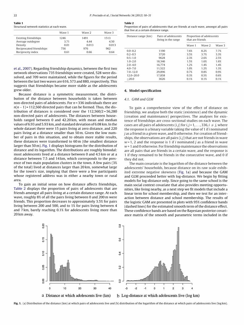

Page 5

22 P. Preciado et al. / Social Networks 34 (2012) 18– 31

Table 1Structural network statistics at each wave.

Wave 1 Wave 2 Wave 3

Existing friendships 1246 1491 1513Average outdegree 3.71 4.44 4.50Density 0.01 0.013 0.013Reciprocated friendships 756 976 962

ensbsg

bnntnhvwpbtldmdeofwa

Tfwfla2

Table 2Proportion of pairs of adolescents that are friends at each wave, amongst all pairsthat live at a certain distance range.

Distance range (km) Pairs of adolescentsliving in the range

Proportion of adolescentsthat are friends

Wave 1 Wave 2 Wave 3

0.0–0.2 1190 7.6% 8.2% 7.7%0.2–0.5 3720 3.5% 3.7% 3.3%0.5–1.0 9628 2.3% 2.6% 2.5%1.0–2.0 18,346 1.5% 1.6% 1.6%2.0–4.0 16,774 1.2% 1.4% 1.4%4.0–7.0 11,522 1.0% 1.2% 1.3%7.0–12.0 29,896 0.7% 0.8% 0.9%

the logistic GAM are presented in plots with 95% confidence bands

F

Reciprocity index 0.61 0.66 0.64

t al., 2007). Regarding friendship dynamics, between the first twoetwork observations 735 friendships were created, 528 were dis-olved, and 709 were maintained, while the figures for the periodetween the last two waves are 616, 573 and 880, respectively. Thisuggests that friendships became more stable as the adolescentsrew older.

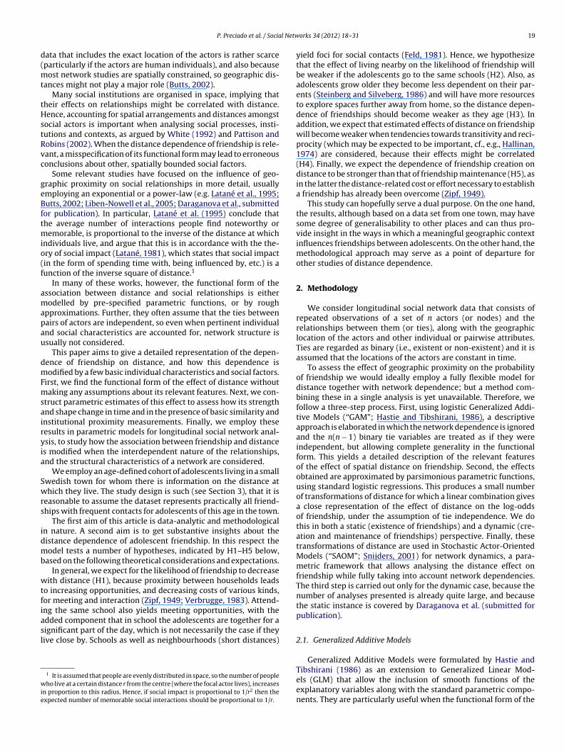
Because distance is a symmetric measurement, the distri-ution of the distance between households is taken betweenon-directed pairs of adolescents. For n = 336 individuals there are(n − 1) = 112,560 directed pairs that can be formed. Thus, the dis-ribution of distances is considered over the 112,560/2 = 56,280on-directed pairs of adolescents. The distances between house-olds ranged between 0 and 42.20 km, with mean and medianalues of 6.93 and 5.93 km, and standard deviation of 6.08 km. In thehole dataset there were 15 pairs living at zero distance, and 220airs living at a distance smaller than 50 m. Given the low num-er of pairs in this situation, and to obtain more stable results,hese distances were transformed to 60 m (the smallest distancearger than 50 m). Fig. 1 displays histograms for the distribution ofistance and its logarithm. The distributions are roughly bimodal:ost adolescents lived at a distance between 0 and 4.5 km or at a

istance between 7.5 and 14 km, which corresponds to the pres-nce of two main population clusters in the town. A few pairs (3%f the total) lived at distances larger than 20 km, somewhat largeor the town’s size, implying that there were a few participantshose registered address was in either a nearby town or rural

rea.To gain an initial sense on how distance affects friendships,

able 2 displays the proportion of pairs of adolescents that areriends amongst all pairs living at a certain distance range. At eachave, roughly 8% of all the pairs living between 0 and 200 m were

riends. This proportion decreases to approximately 3.5% for pairs

iving between 200 and 500, and to 1% for pairs living between 4nd 7 km, barely reaching 0.1% for adolescents living more than0 km away.

ig. 1. (a) Distribution of the distance (km) at which pairs of adolescents live and (b) distr

12.0–20.0 17,858 0.3% 0.5% 0.6%≥20.0 3626 0.1% 0.1% 0.1%

4. Model specification

4.1. GAM and GLM

To gain a comprehensive view of the effect of distance onfriendship, we analyse both the static (existence) and the dynamic(creation and maintenance) perspectives. The analyses for exis-tence of friendships are cross-sectional studies on each wave. Thecases are all pairs of adolescents (i, j) for i, j = 1, . . ., 336, i /= j, wherethe response is a binary variable taking the value of 1 if i nominatedj as a friend in a given wave, and 0 otherwise. For creation of friend-ships, the observations are all pairs (i, j) that are not friends in wavew = 1, 2 and the response is 1 if i nominated j as a friend in wavew + 1 and 0 otherwise. For friendship maintenance the observationsare all pairs that are friends in a certain wave, and the response is1 if they remained to be friends in the consecutive wave, and 0 ifthey did not.

The main covariate is the logarithm of the distance between theadolescents’ households, because distance on its raw scale exhib-ited extreme negative skewness (Fig. 1a) and because the GAMand GLM proceeded better with log-distance. We begin by fittingmodels for log-distance only. Since going to the same school is themain social context covariate that also provides meeting opportu-nities, like living nearby, as a next step we fit models that include alinear term for school membership, and then we test for an inter-action between distance and school membership. The results of

(dashed lines) for the estimated smooth term of the distance effect.These confidence bands are based on the Bayesian posterior covari-ance matrix of the smooth and parametric terms included in the

ibution of the logarithm of the distance at which pairs of adolescents live (log km).

Page 6

P. Preciado et al. / Social Networks 34 (2012) 18– 31 23

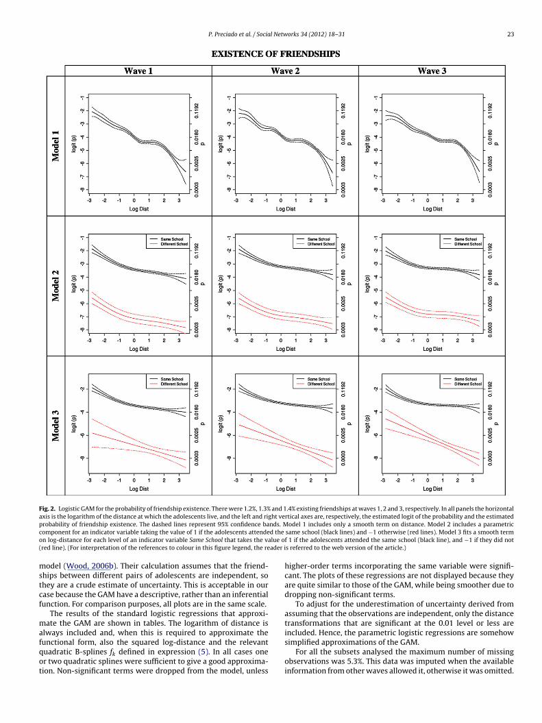
Fig. 2. Logistic GAM for the probability of friendship existence. There were 1.2%, 1.3% and 1.4% existing friendships at waves 1, 2 and 3, respectively. In all panels the horizontalaxis is the logarithm of the distance at which the adolescents live, and the left and right vertical axes are, respectively, the estimated logit of the probability and the estimatedprobability of friendship existence. The dashed lines represent 95% confidence bands. Model 1 includes only a smooth term on distance. Model 2 includes a parametricc d the

o lue o( ader i

mstcf

mafqot

omponent for an indicator variable taking the value of 1 if the adolescents attenden log-distance for each level of an indicator variable Same School that takes the vared line). (For interpretation of the references to colour in this figure legend, the re

odel (Wood, 2006b). Their calculation assumes that the friend-hips between different pairs of adolescents are independent, sohey are a crude estimate of uncertainty. This is acceptable in ourase because the GAM have a descriptive, rather than an inferentialunction. For comparison purposes, all plots are in the same scale.

The results of the standard logistic regressions that approxi-ate the GAM are shown in tables. The logarithm of distance is

lways included and, when this is required to approximate the

unctional form, also the squared log-distance and the relevantuadratic B-splines fk defined in expression (5). In all cases oner two quadratic splines were sufficient to give a good approxima-ion. Non-significant terms were dropped from the model, unless

same school (black lines) and −1 otherwise (red lines). Model 3 fits a smooth termf 1 if the adolescents attended the same school (black line), and −1 if they did nots referred to the web version of the article.)

higher-order terms incorporating the same variable were signifi-cant. The plots of these regressions are not displayed because theyare quite similar to those of the GAM, while being smoother due todropping non-significant terms.

To adjust for the underestimation of uncertainty derived fromassuming that the observations are independent, only the distancetransformations that are significant at the 0.01 level or less areincluded. Hence, the parametric logistic regressions are somehow

simplified approximations of the GAM.

For all the subsets analysed the maximum number of missingobservations was 5.3%. This data was imputed when the availableinformation from other waves allowed it, otherwise it was omitted.

Page 7

24 P. Preciado et al. / Social Networks 34 (2012) 18– 31

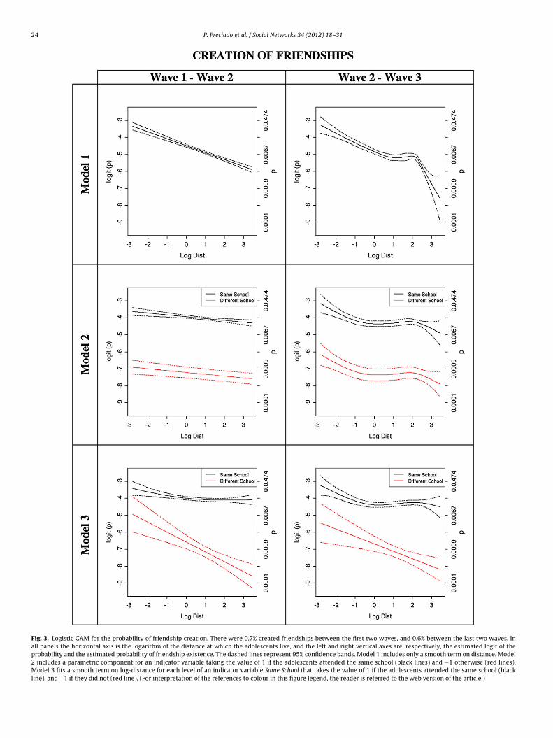
Fig. 3. Logistic GAM for the probability of friendship creation. There were 0.7% created friendships between the first two waves, and 0.6% between the last two waves. Inall panels the horizontal axis is the logarithm of the distance at which the adolescents live, and the left and right vertical axes are, respectively, the estimated logit of theprobability and the estimated probability of friendship existence. The dashed lines represent 95% confidence bands. Model 1 includes only a smooth term on distance. Model2 includes a parametric component for an indicator variable taking the value of 1 if the adolescents attended the same school (black lines) and −1 otherwise (red lines).Model 3 fits a smooth term on log-distance for each level of an indicator variable Same School that takes the value of 1 if the adolescents attended the same school (blackline), and −1 if they did not (red line). (For interpretation of the references to colour in this figure legend, the reader is referred to the web version of the article.)

Page 8

P. Preciado et al. / Social Networks 34 (2012) 18– 31 25

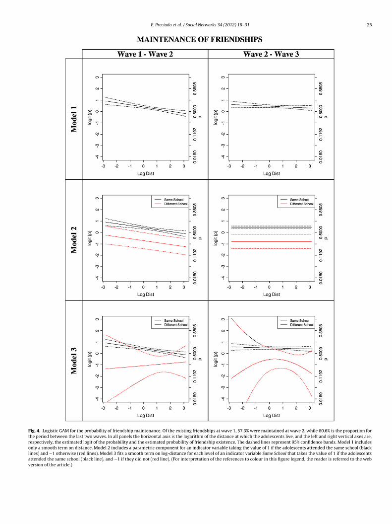
Fig. 4. Logistic GAM for the probability of friendship maintenance. Of the existing friendships at wave 1, 57.3% were maintained at wave 2, while 60.6% is the proportion forthe period between the last two waves. In all panels the horizontal axis is the logarithm of the distance at which the adolescents live, and the left and right vertical axes are,respectively, the estimated logit of the probability and the estimated probability of friendship existence. The dashed lines represent 95% confidence bands. Model 1 includesonly a smooth term on distance. Model 2 includes a parametric component for an indicator variable taking the value of 1 if the adolescents attended the same school (blacklines) and −1 otherwise (red lines). Model 3 fits a smooth term on log-distance for each level of an indicator variable Same School that takes the value of 1 if the adolescentsattended the same school (black line), and −1 if they did not (red line). (For interpretation of the references to colour in this figure legend, the reader is referred to the webversion of the article.)

Page 9

26 P. Preciado et al. / Social Networks 34 (2012) 18– 31

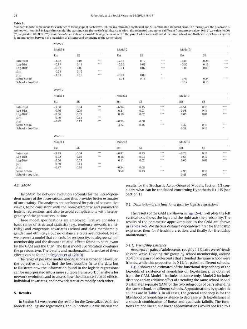
Table 3Standard logistic regressions for existence of friendships at each wave. Est. means estimated coefficient and SE is estimated standard error. The terms fk are the quadratic B-splines with knot in k in logarithmic scale. The stars indicate the level of significance at which the estimated parameter is different from zero: p-value < 0.01 (*), p-value < 0.001(**) or p-value < 0.0001 (***). Same School is an indicator variable taking the value of 1 if the pair of adolescents attended the same school and 0 otherwise. School × Log-Distis an interaction between the logarithm of distance and belonging to the same school.

Wave 1

Model 1 Model 2 Model 3

Est SE Est SE Est SE

Intercept −4.02 0.05 *** −7.15 0.17 *** −6.89 0.24 ***Log-Dist −0.87 0.11 *** −0.26 0.03 *** −0.50 0.13 ***Log-Dist2 −0.07 0.05 0.11 0.02 *** 0.06 0.01 ***f0.00 0.58 0.15 ***f1.00 −1.03 0.19 *** −0.24 0.09 *Same School 3.71 0.16 *** 3.49 0.24 ***School × Log-Dist 0.17 0.13

Wave 2

Model 1 Model 2 Model 3

Est SE Est SE Est SE

Intercept −3.90 0.04 *** −6.94 0.15 *** −6.51 0.19 ***Log-Dist −0.76 0.09 *** −0.21 0.03 *** −0.58 0.11 ***Log-Dist2 −0.06 0.05 0.10 0.02 *** 0.05 0.01 ***f0.00 0.49 0.13 ***f1.00 −0.87 0.17 *** −0.22 0.08 *Same School 3.72 0.15 *** 3.32 0.19 ***School × Log-Dist 0.31 0.11 *

Wave 3

Model 1 Model 2 Model 3

Est SE Est SE Est SE

Intercept −3.89 0.04 *** −6.81 0.13 *** −6.23 0.16 ***Log-Dist −0.72 0.10 *** −0.16 0.03 *** −0.65 0.10 ***Log-Dist2 −0.06 0.05 0.11 0.02 *** 0.06 0.01 ***f0.00 0.49 0.13 ***

.24

.50

4

dowlg

btgwmbte

ttcni

5

M

f1.00 −0.87 0.16 *** −0Same School 3School × Log-Dist

.2. SAOM

The SAOM for network evolution accounts for the interdepen-ent nature of the observations, and thus provides better estimatesf uncertainty. The analyses are performed for pairs of consecutiveaves, to be consistent with the non-parametric and parametric

ogistic regressions, and also to avoid complications with hetero-eneity of the parameters in time.

Three model specifications are employed. First we consider aasic range of structural statistics (e.g., tendency towards transi-ivity) and exogenous covariates (school and class membership,ender and ethnicity), but no distance effects are included. Next,e present a model that controls for reciprocity, outdegree, schoolembership and the distance related-effects found to be relevant

y the GAM and the GLM. The final model specification combineshe previous two. The details and mathematical formulae of theseffects can be found in Snijders et al. (2010).

The range of possible model specifications is broader. However,he objective is not to find the best possible fit to the data buto illustrate how the information found in the logistic regressionsan be incorporated into a more suitable framework of analysis foretwork evolution, and to assess how the distance-related effects,

ndividual covariates, and network statistics modify each other.

. Results

In Section 5.1 we present the results for the Generalized Additiveodels and logistic regressions, and in Section 5.2 we discuss the

0.08 *0.13 *** 2.95 0.16 ***

0.43 0.09 ***

results for the Stochastic Actor-Oriented Models. Section 5.3 con-siders what can be concluded concerning Hypothesis H1–H5 (seeSection 1).

5.1. Description of the functional form by logistic regressions

The results of the GAM are shown in Figs. 2–4. In all plots the leftvertical axis shows the logit and the right axis the probability. Theresults of the parametric approximations to the GAM are shownin Tables 3–5. We discuss distance dependence first for friendshipexistence, then for friendship creation, and finally for friendshipmaintenance.

5.1.1. Friendship existenceAmongst all pairs of adolescents, roughly 1.3% pairs were friends

at each wave. Dividing the group by school membership, around3.5% of the pairs of adolescents that attended the same school werefriends, while this proportion is 0.1% for pairs in different schools.

Fig. 2 shows the estimates of the functional dependency of thelog-odds of existence of friendship on log-distance, as obtainedfrom the GAM. Model 1 includes distance only. Model 2 includesdistance and an additive effect of attending the same school. Model3 estimates separate GAM for the two subgroups of pairs attendingthe same school, or different schools. Approximations by quadratic

splines are in Table 3. In all cases, the general tendency is for thelikelihood of friendship existence to decrease with log-distance ina smooth combination of linear and quadratic falloffs. The func-tions are not linear, but linear approximations would not lead to a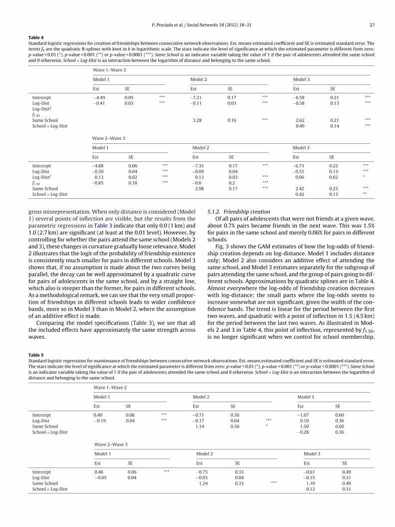

Page 10

P. Preciado et al. / Social Networks 34 (2012) 18– 31 27

Table 4Standard logistic regressions for creation of friendships between consecutive network observations. Est. means estimated coefficient and SE is estimated standard error. Theterms fk are the quadratic B-splines with knot in k in logarithmic scale. The stars indicate the level of significance at which the estimated parameter is different from zero:p-value < 0.01 (*), p-value < 0.001 (**) or p-value < 0.0001 (***). Same School is an indicator variable taking the value of 1 if the pair of adolescents attended the same schooland 0 otherwise. School × Log-Dist is an interaction between the logarithm of distance and belonging to the same school.

Wave 1–Wave 2

Model 1 Model 2 Model 3

Est SE Est SE Est SE

Intercept −4.49 0.05 *** −7.21 0.17 *** −6.58 0.21 ***Log-Dist −0.41 0.03 *** −0.11 0.03 *** −0.58 0.13 ***Log-Dist2

f1.50

Same School 3.28 0.16 *** 2.62 0.21 ***School × Log-Dist 0.49 0.14 ***

Wave 2–Wave 3

Model 1 Model 2 Model 3

Est SE Est SE Est SE

Intercept −4.88 0.06 *** −7.35 0.17 *** −6.73 0.22 ***Log-Dist −0.30 0.04 *** −0.09 0.04 −0.55 0.13 ***Log-Dist2 0.13 0.02 *** 0.13 0.03 *** 0.06 0.02 *

.6

.98

g1p1ca2ispfwAtbo

tw

TSTid

f1.50 −0.85 0.18 *** −0Same School 2School × Log-Dist

ross misrepresentation. When only distance is considered (Model) several points of inflection are visible, but the results from thearametric regressions in Table 3 indicate that only 0.0 (1 km) and.0 (2.7 km) are significant (at least at the 0.01 level). However, byontrolling for whether the pairs attend the same school (Models 2nd 3), these changes in curvature gradually loose relevance. Model

illustrates that the logit of the probability of friendship existences consistently much smaller for pairs in different schools. Model 3hows that, if no assumption is made about the two curves beingarallel, the decay can be well approximated by a quadratic curveor pairs of adolescents in the same school, and by a straight line,hich also is steeper than the former, for pairs in different schools.s a methodological remark, we can see that the very small propor-

ion of friendships in different schools leads to wider confidenceands, more so in Model 3 than in Model 2, where the assumption

f an additive effect is made.

Comparing the model specifications (Table 3), we see that allhe included effects have approximately the same strength acrossaves.

able 5tandard logistic regressions for maintenance of friendships between consecutive networhe stars indicate the level of significance at which the estimated parameter is different frs an indicator variable taking the value of 1 if the pair of adolescents attended the same sistance and belonging to the same school.

Wave 1–Wave 2

Model 1 Model 2

Est SE Est

Intercept 0.40 0.06 *** −0.71

Log-Dist −0.19 0.04 *** −0.17

Same School 1.14

School × Log-Dist

Wave 2–Wave 3

Model 1 Mode

Est SE Est

Intercept 0.46 0.06 *** −0.75Log-Dist −0.05 0.04 −0.03Same School 1.24School × Log-Dist

0.2 ***0.17 *** 2.42 0.23 ***

0.42 0.13 **

5.1.2. Friendship creationOf all pairs of adolescents that were not friends at a given wave,

about 0.7% pairs became friends in the next wave. This was 1.5%for pairs in the same school and merely 0.06% for pairs in differentschools.

Fig. 3 shows the GAM estimates of how the log-odds of friend-ship creation depends on log-distance. Model 1 includes distanceonly; Model 2 also considers an additive effect of attending thesame school, and Model 3 estimates separately for the subgroup ofpairs attending the same school, and the group of pairs going to dif-ferent schools. Approximations by quadratic splines are in Table 4.Almost everywhere the log-odds of friendship creation decreaseswith log-distance; the small parts where the log-odds seems toincrease somewhat are not significant, given the width of the con-fidence bands. The trend is linear for the period between the first

two waves, and quadratic with a point of inflection in 1.5 (4.5 km)for the period between the last two waves. As illustrated in Mod-els 2 and 3 in Table 4, this point of inflection, represented by f1.50,is no longer significant when we control for school membership.

k observations. Est. means estimated coefficient and SE is estimated standard error.om zero: p-value < 0.01 (*), p-value < 0.001 (**) or p-value < 0.0001 (***). Same Schoolchool and 0 otherwise. School × Log-Dist is an interaction between the logarithm of

Model 3

SE Est SE

0.36 −1.07 0.600.04 *** 0.10 0.360.36 * 1.50 0.60

−0.28 0.36

l 2 Model 3

SE Est SE

0.33 −0.61 0.49 0.04 −0.15 0.31

0.33 *** 1.10 0.490.12 0.31

Page 11

2 l Networks 34 (2012) 18– 31

Mawbstptp

5

wpf

f1atgamstBaaite(M

5d

dac

tlmBaTraAies

ncctwe

bt

nce

betw

een

hou

seh

old

s

on

frie

nd

ship

dyn

amic

s,

for

pai

rs

of

con

secu

tive

net

wor

k

obse

rvat

ion

s.

Est.

mea

ns

esti

mat

ed

coef

fici

ent

and

SE

is

its

stan

dar

d

erro

r.

The

star

s

ind

icat

e

the

leve

l of s

ign

ifica

nce

amet

er

is

dif

fere

nt

from

zero

:

p-va

lue

<

0.05

(*),

p-va

lue

<

0.01

(**)

, p-v

alu

e

<

0.00

1

(***

).

Wav

e

1–W

ave

2

Wav

e

2–W

ave

3

Mod

el

1

Mod

el

2

Mod

el

3

Mod

el

1

Mod

el

2

Mod

el

3

Est

SE

Est

SE

Est

SE

Est

SE

Est

SE

Est

SE

21.8

3

1.77

10.1

5

0.51

21.4

4

1.75

17.4

0

1.22

8.51

0.41

17.0

0

1.20

−1.9

9

0.27

***

−3.4

9

0.08

***

−2.4

2 0.

25

***

−2.2

2

0.19

***

−3.3

8

0.07

***

−2.5

7

0.27

***

2.42

0.10

***

2.92

0.07

***

2.43

0.10

***

2.26

0.11

***

2.66

0.07

***

2.28

0.10

***

0.70

0.03

***

0.68

0.03

***

0.62

0.03

***

0.61

0.03

***

−0.5

7

0.06

***

−0.5

7

0.06

***

−0.5

1

0.06

***

−0.5

2

0.06

***

−0.7

4

0.10

***

−0.6

6

0.09

***

−0.7

0

0.08

***

−0.6

2

0.09

***

−0.3

2

0.06

***

−0.2

5

0.06

***

−0.1

5

0.04

***

−0.1

1

0.05

*0.

26

0.04

***

0.27

0.04

***

0.33

0.03

***

0.34

0.04

***

0.57

0.11

***

0.59

0.11

***

0.22

0.09

*

0.22

0.12

0.34

0.05

***

0.37

0.05

***

0.57

0.06

***

0.59

0.05

***

0.73

0.06

***

0.94

0.06

***

0.75

0.07

***

0.62

0.05

***

0.86

0.05

***

0.65

0.06

***

−0.2

3

0.05

***

−0.2

9

0.05

***

−0.2

5

0.05

***

−0.2

9

0.05

***

0.00

0.01

0.00

0.01

0.01

0.01

0.02

0.01

0.15

0.04

***

0.19

0.04

***

0.18

0.04

***

0.20

0.05

***

8 P. Preciado et al. / Socia

odel 2 shows that the likelihood of friendship creation is system-tically smaller for pairs of adolescents in different schools. Whene allow a difference in shape of the distance effect by school mem-

ership as in Model 3, the distance dependence for pairs in the samechool is approximately quadratic, mildly decreasing at small dis-ances but levelling off for distances larger than 1 km; while forairs in different schools it is approximately linear, and strongerhan for pairs in the same school. This pattern is seen at botheriods.

.1.3. Friendship maintenanceAmongst the pairs of adolescents that were friends at a given

ave, approximately 59% remained friends in the next wave. Theseroportions were 61% for adolescents in the same school and 30%or adolescents in different schools.

Fig. 4 presents the GAM estimates of how the log-odds ofriendship maintenance depends on log-distance. Here also, Model

includes distance only, Model 2 adds an additive effect ofttending the same school, and Model 3 presents estimates forhe pairs attending the same school and separately for the pairsoing to different schools. Approximations by quadratic splinesre in Table 5. Fig. 4 shows that the log-odds of friendshipaintenance decreases linearly with log-distance in all model

pecifications for the period between the first two waves, andhat there is no dependence on distance for the second period.elonging to different schools decreases significantly the prob-bility of friendship maintenance (Model 2). Note that whenn interaction between school membership and log-distance isncluded (Model 3), all terms become insignificant. This is becausehere are very few cases for friendship maintenance in differ-nt schools and the estimations are unreliable for this groupFig. 4, bottom row). Hence Model 2 here is more meaningful than

odel 3.

.2. Assessing the effect of geographic proximity on friendshipynamics

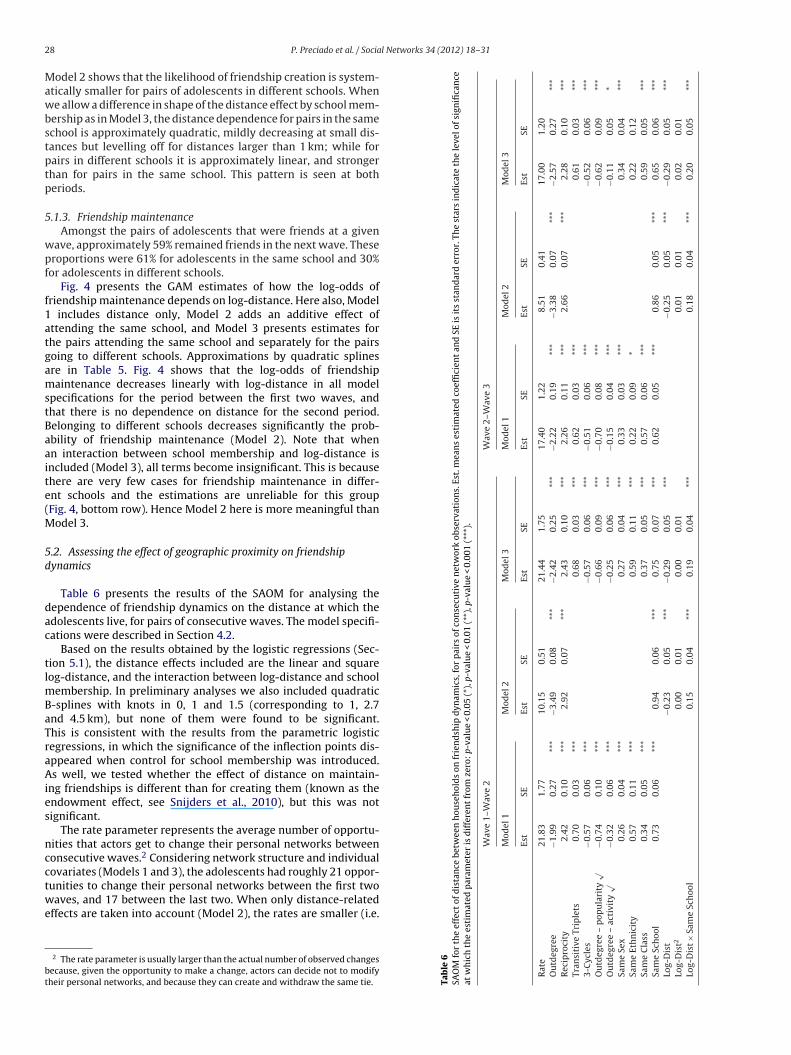
Table 6 presents the results of the SAOM for analysing theependence of friendship dynamics on the distance at which thedolescents live, for pairs of consecutive waves. The model specifi-ations were described in Section 4.2.

Based on the results obtained by the logistic regressions (Sec-ion 5.1), the distance effects included are the linear and squareog-distance, and the interaction between log-distance and school

embership. In preliminary analyses we also included quadratic-splines with knots in 0, 1 and 1.5 (corresponding to 1, 2.7nd 4.5 km), but none of them were found to be significant.his is consistent with the results from the parametric logisticegressions, in which the significance of the inflection points dis-ppeared when control for school membership was introduced.s well, we tested whether the effect of distance on maintain-

ng friendships is different than for creating them (known as thendowment effect, see Snijders et al., 2010), but this was notignificant.

The rate parameter represents the average number of opportu-ities that actors get to change their personal networks betweenonsecutive waves.2 Considering network structure and individualovariates (Models 1 and 3), the adolescents had roughly 21 oppor-

unities to change their personal networks between the first twoaves, and 17 between the last two. When only distance-related

ffects are taken into account (Model 2), the rates are smaller (i.e.

2 The rate parameter is usually larger than the actual number of observed changesecause, given the opportunity to make a change, actors can decide not to modifyheir personal networks, and because they can create and withdraw the same tie. Ta

ble

6SA

OM

for

the

effe

ct

of

dis

taat

wh

ich

the

esti

mat

ed

par

Rat

e

Ou

tdeg

ree

Rec

ipro

city

Tran

siti

ve

Trip

lets

3-C

ycle

s

Ou

tdeg

ree

–

pop

ula

rity

√O

utd

egre

e

–

acti

vity

√Sa

me

Sex

Sam

e

Eth

nic

ity

Sam

e

Cla

ss

Sam

e

Sch

ool

Log-

Dis

tLo

g-D

ist2

Log-

Dis

t ×Sa

me

Sch

ool

Page 12

l Netw

1ttpa

ntn(3tsinntht

tpGiccfstsTawes

oralttfpjssfhts

tcdaids

eanfaa

P. Preciado et al. / Socia

0 and 8.5), which happens because between consecutive waveshere are fewer changes in terms of the few, distance-related effectshan in terms of a wider range of statistics. The difference betweeneriods suggests the friendships are slightly more stable when thedolescents grow older.

All model specifications confirm a few known aspects of theature of adolescent friendships. There is a strong tendencyowards reciprocity (the reciprocity parameter is positive and sig-ificant), and evidence for transitive closure and local hierarchybecause the transitive triplets parameter is positive, while the-cycle parameter is negative). As well, the adolescents favour rela-ionships in their same class and school, and with others of theame gender. The preference for friendships of the same ethnicitys important in the first period but irrelevant in the second. Theegative outdegree-popularity effect shows that adolescents thatominate many friends are less likely to be chosen as friends, whilehe negative outdegree-activity effect reflects that adolescents withigher outdegrees at a given moment are less likely to create newies subsequently.

The reading of the log-distance effects can be done from eitherhe second or third model specifications, because the estimatedarameters are rather similar. In contrast to the GAM and theLM results, the quadratic effect of distance is not significant. To

nterpret the numerical values of the parameters, it should beonsidered that attending the same school is represented by aentred dummy variable. Due to the centring, its values are 0.6or attending the same school and −0.4 for attending differentchools. Ignoring the non-significant and small quadratic term,he resulting effect of log-distance for those attending the samechool is −0.18, and for those attending different schools −0.37.he numbers are practically the same for both periods. These neg-tive coefficients imply that the adolescents favour relationshipsith others that live close to them, while the magnitude of this

ffect is about twice as large if the adolescents go to differentchools.

To further interpret the numerical value of the estimatebtained for the effect of distance, we can calculate the probabilityatio of an adolescent i choosing to create a friendship with onedolescent j that lives at a log-distance d from i, over another ado-escent h that lives at d + ln(2), if j and h are equal with respecto i in all the other characteristics. Succinctly formulated, this ishe effect of doubling the distance between the households onriendship creation. Using expression (8) we obtain that, at botheriods, the probability of choosing to create a friendship with

is 1.13 times larger than with h if i, j and h go to the samechool, and 1.30 times larger if neither j nor h attend the samechool as i. Within the town, distances can be much more than aactor of 2 apart. Hence, the effect of geographic proximity betweenouseholds is strong and relevant when the adolescents do not goo the same school, but rather small when they do attend the samechool.

A comparison between Models 1 and 3 shows that most ofhe estimated parameters of the structural characteristics andovariates are not importantly modified by the inclusion of theistance-related effects. Thus, the proximity between householdsccounts for a different aspect of the friendship dynamics, whichs most remarkable for the triadic effects, entailing that geographicistance has a different dimension than social distance (at least forocial configurations of three actors).

Analogously, a parallel assessment of the second and third mod-ls shows that the estimated reciprocity and same school effectsre attenuated when including other structural characteristics and

otions of similarity between individuals. The parameter estimates

or the log-distance effects are nearly the same in Models 2 and 3t both periods, confirming that the distance between-householdsccounts for an aspect of friendship dynamics that cannot be

orks 34 (2012) 18– 31 29

explained by other basic individual characteristics and measuresof network structure.

5.3. The results in the light of initial expectations

At the end of Section 1 five hypotheses, H1–H5, were presented.We discuss these in turn.

We found clear evidence for a negative effect of distance on theexistence of friendship ties (Fig. 2) and on the creation of friendshipties (Fig. 3); for maintenance of friendship (Fig. 4), there was aneffect only in the first period of the study (mainly 13 going to 14years) but not in the second period (14 going to 15). In the dynamicmodel (SAOM) for friendship too (Table 6), there was an evidentdistance effect. This supports hypothesis H1, with the exceptionof the case of friendship maintenance for the age range of middleadolescence (14 to 15 years).

Going to the same school likewise had a strong effect on friend-ship, and this interacted with distance as expected according tohypothesis H2: for those going to different schools, living nearby ismore important than for those going to the same school. Fig. 2,Model 3, shows this for friendship existence, with a differencein slopes mainly for distances larger than 1 km. Fig. 3, Model 3,shows this for creation of new friendships. For maintenance offriendships the effect is not significant, which may be due tothe low number of friendships in different schools. The dynamicmodel also supported this interaction hypothesis (Table 6, Models 2and 3).

For those attending the same school, distances have an effectmainly below 350 m (log-distance less than −1; Figs. 2 and 3, Model3). For larger distances the slope of the logit becomes negligible,and practically null after 1 km (log-distances larger than 0). Thisplateau suggests that having an institutional setting, in which theadolescents spend a significant part of the day, provides meetingopportunities and a social focus (Feld, 1981) comparable to liv-ing nearby. In this context, it would be interesting to assess if thesame phenomenon occurs for other institutional settings, such asorganised activities.

The findings with respect to the expected attenuation ofdistance effects as adolescents get older were ambiguous. The non-linear nature of the effect of distance make it more difficult to evenformulate this as an unequivocal hypothesis for a given parameter,but it can be visually assessed by comparing the results for Waves1–2 to those for Waves 2–3. Figs. 2 and 3 suggest that over thislimited age range there is little change in the effect of distance onexistence or on creation of friendship ties. Table 5 (Models 1–2)shows evidence that distance is less important for maintenance offriendships in the 14–15 years age range than in the 13–14 agerange. The SAOM results gave no support for decreasing impor-tance of distance when adolescents get older. Together, this is avery partial confirmation of hypothesis H3.

The expectation that accounting for network dependencies,such as transitive closure, would decrease the estimated effectsof distance (H4), was not supported at all, as can be seen fromTable 6 when comparing Models 2 and 3. The correlations betweenthe parameter estimates for the distance effect and the parametereffects for structural network effects in the SAOM all were less inabsolute value than 0.2. The distance effect was correlated withthe effect of going to the same school, and taking distance intoaccount reduced the effect of attending the same school by aboutone quarter of its initial value.

As expected, the effect of distance on friendship creation was

clearly stronger than on friendship maintenance, as can be seenfrom comparing Figs. 3 and 4. Unfortunately, we were not able toobtain converging parameter estimates when trying to test this inthe SAOM.

Page 13

3 l Netw

6

oepd

iMfocdoTmrfdcF

etftwiseaot

l

wtrtspiviu

deldjw(iTmemc

otdic

0 P. Preciado et al. / Socia

. Discussion

The objective of this paper was to give an accurate descriptionf the functional form of the distance dependence of friendshipxistence, creation, and maintenance. In addition, we aimed atroposing a methodology that can be employed when studying theistance dependence of network dynamics.

We analysed a three-wave network of 336 adolescents liv-ng in a small Swedish town. First, we used Generalized Additive

odels (GAM; Hastie and Tibshirani, 1986) to assess the relevanteatures of the association between distance and friendship, with-ut making rigid assumptions about its parametric form. Next, weonstructed parametric approximations of these results using stan-ard logistic regressions. A first model only considered the effectf log-distance between households on the log-odds of friendship.hen we assessed how the strength and shape of this effect wereodified by school membership. Finally, we employed the logistic

egression results in estimating stochastic actor-oriented modelsor network evolution (SAOM; Snijders, 2001), to compare howistance affects the dynamic of friendship when basic individualovariates and network structural characteristics are considered.ive hypotheses were formulated and tested.

A general descriptive result is that, as expected, there was a clearffect of distance on the existence and creation of friendships, andhis could be represented very well by modelling the log-odds ofriendship existence, and of friendship creation, as a smooth func-ion of the logarithm of distance; a linear function of log-distanceas in all cases at least a quite reasonable approximation, and

n some cases the best representation. When in a logistic regres-ion the estimated probabilities are small (such as for creation andxistence of friendships), the logit is well approximated by the log-rithm. If for these cases the log-odds of friendship depends linearlyn log-distance, we obtain a power-law dependence of probabili-ies on distance, because

ogit(p) = ˇ0 + ˇ1 log(dist) ⇒ p ≈ ˛0 distˇ1 (9)

here ˛0 = exp(ˇ0). Hence, the probability of friendship is propor-ional to distˇ1 . We obtained estimated values of ˇ1 roughly in theange between –0.7 and –0.2. The proportionality to inverse dis-ance (ˇ1 = −1) or inverse distance squared (ˇ1 = −2), proposed byome authors (e.g., Latané et al., 1995; Butts, 2002) is not at all sup-orted by our results. We think that, when probability of friendship

s approximately proportional to a power of distance, the precisealue of this power will depend on various aspects of the context,ncluding the range of distances under consideration, in our casep to 20 km; at larger distances different processes will play a role.

The results from the GAM and logistic regression analysis areescriptive of distance dependence of friendship and were gen-rally supportive of our hypotheses (Section 5.3): friendships getess probable as distances increase; the importance of living nearbyecreases when there are other social foci such as in our case the

oint attendance of a school; the importance of distance may geteaker as adolescents get older, but in our restricted age range

13–15 years mainly) this was supported only weakly; and distances more important for creating than for maintaining friendships.hese results, although obtained here for one specific case of aedium-sized town in Sweden, are qualitatively in line with gen-

ral considerations, and we think that they will retain their validityore widely for the probability of real friendships amongst adoles-

ents in geographically bounded regions.The smooth dependence of the log-odds of friendship creation

n log-distance led us to using logarithmically transformed dis-

ance in a more encompassing network model (SAOM) of friendshipynamics, also representing network dependencies. The irregular-

ties in the dependence of friendship on log-distance, presumablyonnected to the spatial layout of the town, already were smoothed

orks 34 (2012) 18– 31

out when controlling for attending the same school (as shown bythe differences between Models 1 and 2 in Figs. 2–4) and werefurther reduced in the SAOM, where only a linear effect of log-distance was significant. Thus, the non-parametric GAM analysiswas a useful first step to suggest a transformation of distance inthe parametric SAOM approach. In our case, the use of distance inthe SAOM led to different estimates for effects of other foci such asschool, but not to important differences in parameter estimates fortriadic or degree-related structural effects.

It is debatable that the distance between households “as thecrow flies” is the best way to account for real geographic prox-imity and accessibility. These aspects will usually depend on theavailability of transportation and communication technologies, thepopulation density, level of urbanisation, and the town’s topology.In this sense, we cannot expect our findings to extend to cities ortowns with very different characteristics to the one studied. Never-theless, by using the shortest spatial distance between householdswe still found important and well-interpretable results. This sug-gests that indeed the geographic proximity between social actorsis relevant for friendship networks that are relatively constrainedin space, although more detailed measurements of the constraintsand possibilities offered by distance may be useful to capture fur-ther important features of the effects of space and distance on socialrelationships.

Acknowledgements

We thank Ruth Ripley, Rasmus Lechedahl Petersen and JamesReeve for their support and advice.

References

Blau, P.M., Schwartz, J.E., 1984. Crosscutting Social Circles: Testing A MacrostructuralTheory of Intergroup Relations. Academic Press, Orlando, FL.

Burk, W.J., Kerr, M., 2008. The co-evolution of early adolescent friendship networks,school involvement, and delinquent behaviors. Revue Franc aise de Sociologie,499–522.

Burk, W.J., Steglich, C.E.G., Snijders, T.A.B., 2007. Beyond dyadic interdependence:actor-oriented models for co-evolving social networks and individual behaviors.International Journal of Behavioral Development 31, 397–404.

Butts, C.T., 2002. Spatial models of large-scale interpersonal networks. DoctoralDissertation. Carnegie Mellon University.

Carley, K.M., Wendt, K., 1991. Electronic mail and scientific communication: a studyof the Soar Extended Research Group. Knowledge: Creation, Diffusion, Utiliza-tion 12, 406–440.

Carrasco, J.A., Hogan, B., Wellman, B., Miller, E.J., 2008. Agency in social activityinteractions: the role of social networks in time and space. Tijdschrift vooreconomische en sociale geografie 99, 562–583.

Cohen, J., 1997. Sources of peer group homogeneity. Sociological Education 50,227–241.

Daraganova, G., Pattison, P., Mitchell, B., Anthea, B., Watts, M., Baum, S. Networksand geography: modelling community network structures as the outcome ofboth spatial and network processes. Social Networks, submitted for publication,doi:10.1016/j.socnet.2010.12.001.

Dijst, M., 2006. ICT and Social Networks: towards a situational perspective on theinteraction between corporeal and connected presence. In: 11th InternationalConference on Travel Behaviour Research , Kyoto, August 16–20, 2006.

Feld, S.L., 1981. The focused organization of social ties. American Journal of Sociology86, 1015–1035.

Feld, S.L., 1982. Social structural determinants of similarity among associates. Amer-ican Sociological Review 47, 797–801.

Gest, S.D., Davidson, A.J., Rulison, K.L., Moody, J., Welsh, J.A., 2007. Features of groupsand status hierarchies in girls’ and boys’ early adolescent peer networks. NewDirections for Child and Adolescent Development 118, 43–59.

Green, P.J., Silverman, B.W., 1994. Nonparametric Regression and Generalized LinearModels: A Roughness Penalty Approach. Chapman & Hall, London.

Hallinan, M.T., 1974. A structural model of sentiment relations. The American Journalof Sociology 80, 364–378.

Hastie, T., Tibshirani, R., 1986. Generalized additive models (with discussion). Sta-tistical Science 1, 297–318.

Hastie, T., Tibshirani, R., 1990. Generalized Additive Models. Chapman & Hall, New

York.

Kandel, D.B., 1978. Homophily, selection, and socialization in adolescent friendships.American Journal of Sociology 84, 427–436.

Latané, B., 1981. The psychology of social impact. American Psychologist 36,343–356.

Page 14

l Netw

L

L

L

L

M

M

P

R

S

S

P. Preciado et al. / Socia

atané, B., Liu, J.H., Nowak, A., Bonevento, M., Zheng, L., 1995. Distance matters:physical space and social impact. Personality and Social Psychology Bulletin 21,795–805.

azarsfeld, P., Merton, R.K., 1954. Friendship as a social process: a substantive andmethodological analysis. In: Freedom and Control in Modern Society. Van Nos-trand, New York, pp. 18–66.

iben-Nowell, D., Novak, J., Kumar, R., Raghavan, P., Tomkins, A., 2005. Geographicrouting in social networks. Proceedings of the National Academy of Sciences ofthe United States of America 102, 11623–11628.

ieberson, S., 1980. A Piece of the Pie: Blacks and White Immigrants Since 1880.Univ. of California Press, Berkeley.

cCullagh, P., Nelder, J.A., 1989. Generalized Linear Models, 2nd ed. Chapman &Hall/CRC, Boca Raton, FL.

cPherson, M., Smith-Lovin, L., Cook, J.M., 2001. Birds of a feather: homophily insocial networks. Annual Review of Sociology 27, 415–444.

attison, P., Robins, G., 2002. Neighborhood-based models for social networks. Soci-ological Methodology 32 (1), 301–337.

ipley, R.M., Snijders, T.A.B., 2010. Manual for SIENA Version 4. 0. University ofOxford, Department of Statistics; Nuffield College, Oxford.

eber, G.A.F., Wild, C.J., 1989. Nonlinear Regression. John Wiley & Sons, New York,NY.

nijders, T.A.B., 2001. The statistical evaluation of social network dynamics. In:Sobel, M., Becker, M. (Eds.), Sociological Methodology. Basil Blackwell, Bostonand London, pp. 361–395.

orks 34 (2012) 18– 31 31

Snijders, T.A.B., 2005. Models for longitudinal network data. In: Carrington, P.J.,Scott, J., Wasserman, S. (Eds.), Models and Methods in Social Network Analysis.Cambridge University Press, New York, pp. 215–247.

Snijders, T.A.B., van de Bunt, G.G., Steglich, C.E.G., 2010. Introduction to stochasticactor-based models for network dynamics. Social Networks 32, 44–60.

Steinberg, L., Silveberg, S.B., 1986. The vicissitudes of autonomy in early adolescence.Child Development 57 (4), 841–851.

Tsai, M.C., 2006. Sociable resources and close relationships: intimate relativesand friends in Taiwan. Journal of Social and Personal Relationships 23,151–169.

Verbrugge, L.M., 1983. A research note on adult friendship contact: a dyadic per-spective. Social Forces 62, 78–83.

Wellman, B., 1996. An electronic group is virtually a social network. In: Kiesler, S.,Hillsdale, N.J. (Eds.), Research Milestones on the Information Highway. LawrenceErlbaum Associates, Inc., Hillsdale, NJ.

White, H.C., 1992. Identity and Control: How Social Formations Emerge. PrincetonUniversity Press, Princeton, NJ.

Wood, S.N., 2006a. Generalized Additive Models: An Introduction with R. Chapman& Hall/CRC, Boca Raton, FL.

Wood, S.N., 2006b. On confidence intervals for generalized additive models basedon penalized regression splines. Australian & New Zealand Journal of Statistics48, 445–464.

Zipf, G.K., 1949. Human Behavior and the Principle of Least Effort. Addison Wesley,Menlo Park, CA.