Does Income Growth Relocate Ecological Footprint?

Does Income Growth Relocate Ecological

Footprint?

Ahmet Atıl Aşıcı*

Sevil Acar**

(June 2015)

Abstract

The aim of this paper is to investigate whether countries tend

to relocate their ecological footprint as they grow richer. The

analysis is carried out for a panel of 116 countries by

employing the production and import components of the

Ecological Footprint data of the Global Footprint Network for

the period 2004-2008. With few exceptions, the existing

Environmental Kuznets Curve (EKC) literature concentrates only

on the income-environmental degradation nexus in the home

country and neglects the negative consequences of home

consumption spilled out. Controlling for the effects of

openness to trade, biological capacity, population density,

industry share and energy per capita as well as stringency of

environmental regulation and environmental regulation

1

enforcement, we detect an EKC-type relationship only between

per capita income and footprint of domestic production. Within

the income range, import footprint is found to be monotonically

increasing with income. Moreover, we find that domestic

environmental regulations do not influence country decisions to

import environmentally harmful products from abroad; but they

do affect domestic production characteristics. Hence, our

findings indicate the importance of environmental regulations

and provide support for the “Pollution Haven” and “Race-to-the-

Bottom” hypotheses.

Keywords: Ecological footprint, Economic growth, Environmental

Kuznets Curve, Environmental Regulation

JEL codes: Q01, Q56, Q57

* Corresponding Author. Assoc. Prof., Istanbul Technical University, Department of Management Engineering. Address: Istanbul Technical University, Faculty of Management

34367 Maçka, İstanbul, TURKEYE-mail: [email protected] Phone: +90 212 293 1300 / 2050 /203Fax: +90 212 224 8685

2

** Assoc. Prof., Istanbul Kemerburgaz University, Department ofEconomics.Address: Istanbul Kemerburgaz University, Department of Economics

Mahmutbey Dilmenler Cad. No: 26, Bağcılar, İstanbul, TURKEY

E-mail: [email protected]: +90 212 604 01 00 / 4064Fax: +90 212 445 92 55

1. Introduction

This paper intends to detect whether countries tend to export

negative environmental consequences of their consumption as

they grow richer, and uncover the factors that drive such

3

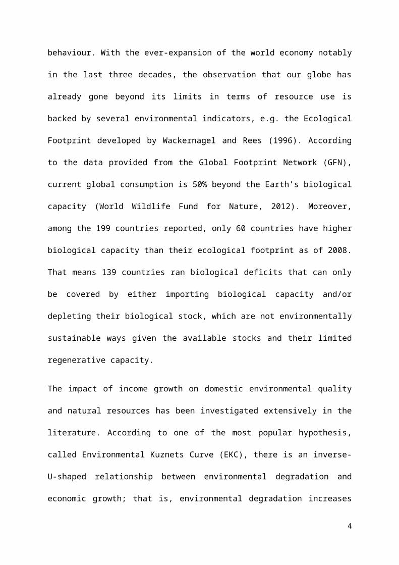
behaviour. With the ever-expansion of the world economy notably

in the last three decades, the observation that our globe has

already gone beyond its limits in terms of resource use is

backed by several environmental indicators, e.g. the Ecological

Footprint developed by Wackernagel and Rees (1996). According

to the data provided from the Global Footprint Network (GFN),

current global consumption is 50% beyond the Earth’s biological

capacity (World Wildlife Fund for Nature, 2012). Moreover,

among the 199 countries reported, only 60 countries have higher

biological capacity than their ecological footprint as of 2008.

That means 139 countries ran biological deficits that can only

be covered by either importing biological capacity and/or

depleting their biological stock, which are not environmentally

sustainable ways given the available stocks and their limited

regenerative capacity.

The impact of income growth on domestic environmental quality

and natural resources has been investigated extensively in the

literature. According to one of the most popular hypothesis,

called Environmental Kuznets Curve (EKC), there is an inverse-

U-shaped relationship between environmental degradation and

economic growth; that is, environmental degradation increases

4

as income increases up to an income threshold and starts to

fall. In the majority of the EKC studies, a one-dimensional

environmental quality indicator (such as CO2 emissions, waste,

etc.) has been employed and the effects of income on the

environment have been measured in the country where production

and consumption take place. Yet, it is clear that the effects

of economic activities on environmental quality are multi-

dimensional rather than one-dimensional. Moreover, in today’s

globalized world, locations of production and consumption have

been changing rapidly. This necessitates the measurement of

environmental degradation and natural resource exploitation not

only in the location where consumption takes place but also in

the production location given the fact that international trade

and capital flows make it possible to import rather than

produce domestically the goods which are ecologically

destructive (Peters et al., 2011; Weinzettel et al., 2013).

Previous EKC literature brings us to the discussion of whether

the EKC relationship is quasi-automatic or policy-induced

(Grossman et al. 1995; Van Alstine and Neumayer, 2010). Heavy

regulation at home may force companies to adopt cleaner

technologies at home and/or force dirty industries to migrate

5

abroad where regulations are laxer. Apart from these push

factors, it is also observed that many developing countries are

forced to lower their environmental standards in the aim to

gain international competitiveness and to attract foreign

direct investments which are perceived as essential for

sustaining economic growth. Therefore, it is plausible to think

that increasing environmental quality in a rich country could

be gained at the expense of degrading environmental quality

abroad. In other words, from a global perspective, an EKC-type

relationship at home does not necessarily imply that domestic

consumption patterns have been put back on an environmentally

sustainable path. By importing rather than producing those

goods causing environmental degradation, a society can simply

continue its “unsustainable” life-style (Schütz et al., 2004;

Mayer et al., 2005; Berlik et al., 2002).

In this paper, we deal with these two less frequently addressed

topics in the EKC literature. First, we focus on the

multidimensional property of environmental degradation and

natural resource use. Second, we distinguish between

environmental pressures created in the domestic economy versus

abroad. We employ the multi-dimensional Ecological Footprint

6

data to measure environmental quality and natural resource

depletion with a panel fixed-effects analysis to detect the

relationship between income and footprints that result from

domestic production and imports for 116 countries in the period

2004-2008 within the EKC framework. Ecological footprint data

enable to track the effect of income on domestic and foreign

biological capacities and hence provide a better understanding.

Moreover, as a multi-dimensional indicator, ecological

footprint might help us to portray a more general picture.

The outline of the paper is as follows. The following section

reviews the relevant literature. The third section describes

the data and the model used. In section four, we report the

regression results, and finally, section five concludes.

2. Background and Relevant Literature

The EKC hypothesis suggests that the effects of economic growth

or income on the environment are carried out through three

channels called the “scale”, “composition and “technology”

channels. The pioneering study by Grossman and Krueger (1991)

asserts that the negative scale effect (increasing consumption

due to increasing affluence) tend to prevail in the initial

7

stages of economic growth, but after a threshold level of

development it should be outweighed by the change in the

composition of production (shift toward cleaner sectors) and by

the change in technology employed (shift toward cleaner

technologies). Following this study, numerous studies have been

conducted in search of the existence of an EKC in different

countries using various environmental quality indicators. Yet

the empirical evidence is mixed; that is, it is not possible to

assume a unique curve for all types of environmental

degradation (see Dinda (2004) and Carson (2010) for a critical

survey of the recent EKC literature). Whether it exists or not,

the question which the majority of the EKC studies leave

unanswered is whether environmental pressure is decoupled from

income growth on the global scale or not.

In contrary to the bulk of the literature that focuses on

single pollution indicators to investigate the EKC hypothesis,

there are a limited number of studies that address the

consumption-based approach to the EKC. Among them, Bagliani et

al. (2008) utilize ecological footprint data for 141 countries

in 2001 and conduct Ordinary Least Squares and Weighted Least

Squares analysis on linear, quadratic and cubic functions, in

8

standard and logarithmic specifications, as well as a

nonparametric regression. Their results suggest that using

ecological footprint as a dependent variable does not reveal an

EKC-type relationship. Instead they find that environmental

pressure is intensified as income per capita increases. These

findings are supported by both York et al. (2004) and Caviglia

et al. (2009), who emphasize that ecological footprint rises

significantly with gross domestic product (GDP) per capita. Al-

mulali et al. (2015: 315) point out that the EKC “only occurs

in a stage of economic development in which technologies are

available that improve energy efficiency, energy saving and

renewable energy” in their panel analysis of 93 countries. Chen

et al. (2010), on the other hand, examine the relationship

between ecological footprint and social development level

rather than GDP per capita and fail to evidence an inverted U-

shaped relationship. Most of these studies do not make use of

relevant control variables such as industry share and

environmental regulation in search for this relationship where

as our analysis contributes to the literature by acknowledging

the importance of various factors other than income.

9

An increase in environmental quality after a certain level of

income (hence an EKC-type of turn) at home can easily be

achieved without altering the unsustainable consumption

patterns thanks to the increasing international trade and

capital flows. Andersson and Lindroth (2001) lists four

different ways of how trade may affect ecological footprint:

(a) positive allocative effect, which reduces ecological footprint

as trade enables specialization of countries on products which

are produced with a higher yield, (b) negative income effect,

which increases ecological footprint as trade helps countries

raise their income, and thereby, consumption, (c) negative rich-

country-illusion effect, which highlights the false impression in rich

countries that their lifestyle is sustainable which might be

formed thanks to the possibility of importing bio- and sink-

capacity from poorer countries, and (d) negative terms-of-trade

distortion effect, which hints to the tendency of poorer countries

to exploit natural resources beyond sustainable scales to

protect themselves from falling terms-of-trade during boost

periods in world demand.

The possibility of importing bio- and sink-capacity with rising

income also creates another illusion on the side of poor

10

countries that economic growth is the necessary condition for a

better environment (Nordström and Vaughan, 1999). This, at the

end, causes ecological footprint to climb up both in rich and

poor countries. Therefore, it is indispensable to consider the

effects of international trade when dealing with income-

environmental quality relationship a la EKC. This is where this

paper departs from others: analysing separately the effect of

income (after controlling for several factors) on ecological

footprints caused by domestic production and imports.

The positive effects unleashed by increasing income in richer

countries (through channels of composition, technology and

increasing sensitivity reflected in tightened regulations)

could help to clean up the domestic environment; but this does

not guarantee an overall reduction in environmental degradation

globally, if not an increase. There are several ways of

importing environmental burden of consumption in rich countries

that can be understood in the context of “unequal ecological

exchange” among countries (Andersson and Lindroth, 2001). One

explanation is that less developed countries extract natural

resources and export them to more developed ones so that the

latter externalize pollution and environmental costs by means

11

of importing resource-intensive goods or energy materials.

Schütz et al. (2004) describes how improvements in the motor-

car emission technology, possibly triggered by tightened

regulation in the EU countries, relocate polluting production

processes in the form of ecological rucksacks and how such

relocation increases pollution. They find that the pressure on

the environment due to “ecological rucksack” of the EU imports

from developing countries stood at 5 to 1: that is, one tonne

of imported raw materials resulted in 5 tonnes of erosion or

unused extraction material in the countries of origin, whereas

imports from newly industrializing countries in Europe carried

a burden of only 1.6 tonnes rucksack per tonne of raw materials

in the year 2000. Similarly, Peters et al. (2011) show that

Annex B countries of the Kyoto Protocol (countries with

emissions reduction obligations) have dislocated an increasing

share of their CO2 emissions to countries without obligations.

It is plausible to think that available biocapacity in the home

country will also affect the relationship between income and

production and import footprints. Given the level of income,

one could expect to observe a higher concern for environmental

degradation at home where pollution, congestion and resource

12

scarcity are more threatening (Bagliani et al., 2008; Wang et

al., 2013). Additionally, the effects of industry share and

energy use per capita could be controlled for in determining

the relocation of ecological footprint with respect to income.

In line with the EKC hypothesis, one would expect that a higher

share of industry in the economy causes increased environmental

impact and a shift from heavy-industries to services reverts

the impact in favour of the environment. Besides, there are

also arguments such that industrialization could improve

environmental quality if market forces drive industries to

become more efficient and to reduce not only resource use but

also waste (Mol, 1995; Ozler and Obach, 2009). The impact of

energy use, on the other hand, has been investigated by several

studies such as Atici (2009), which finds that higher energy

use in Central and Eastern Europe generates higher levels of

emissions due to the use of environmentally hazardous energy.

Similar results in the long run are evidenced for the case of

Iran in a study by Saboori and Soleymani (2011). On the other

hand, Caviglia et al. (2009) test the EKC hypothesis performing

a panel data analysis using the ecological footprint of

consumption and find that energy is largely responsible for the

13

lack of an EKC relationship. They find a statistically

significant EKC only when the energy component of the footprint

indicator is removed from the data.

The effect of environmental regulation on economic activity has

been a widely debated policy issue in previous literature.

Heyes (2000) argues that increase in the stringency of

regulations raises incentives for non-compliance, which then

entails the need to enforce them. Cheng and Lai (2012), on the

other hand, argues that a stricter enforcement policy adds to

the financial burden of polluting rms, which then leads thesefi

firms to exert higher political pressure (lobbying) to relax

the environmental standards, consequently creating more

environmental degradation. Some studies advocate that

international trade and foreign direct investment favour

countries with clearly defined environmental regulations. For

instance, analyzing a data set of 29,303 observations from 94

European Fortune Global 500 companies that operate across 77

countries, Rivera and Oh (2013: 243) find that multinational

firms are eager to choose to penetrate into countries with

clearer and stable regulations than their home countries during

the period 2001–2007. There is a vast literature on the link

14

between regulatory characteristics and location of production

investigating the so-called “Pollution Haven”, “Race-to-the-

Bottom” (Daly, 1993; Frankel and Rose, 2005), and “Gains-from-

Trade” (Eskeland and Harrison, 2002) hypotheses. While it is

intuitively plausible to think that environmental regulations

change trade patterns and production locations, empirical

evidence is mixed. Some studies find no link between stringency

of environmental regulation1 and trade in polluting industries

(see Tobey, 1990; Jaffe et al., 1995; and Janicke et al.,

1997). Al-mulali and Tang (2013) find no evidence in favour of

the pollution haven hypothesis in the Gulf Cooperation Council

countries owing to the fact that foreign direct investment to

these countries brings together advanced and eco-friendly

technologies, thereby reducing pollution levels. On the other

hand, Kearsley and Riddel (2010: 905) demonstrate “little

evidence that pollution havens play a significant role in

shaping the EKC”. Yet some others find evidence of the

pollution haven hypothesis (Mani and Wheeler, 1998; Lucas et

al. 1992; Birdsall and Wheeler, 1993). The arguments put

forward by those opposing the pollution haven hypothesis are1 Stringency of environmental regulation data is derived from the questionof “How would you assess the stringency of your country’s environmentalregulations?” included in the World Economic Forum’s Executive OpinionSurvey. See Table A1 for more detail.

15

based on (i) the finding that environmental compliance costs

are often minimal as a proportion of a firm’s total cost

(Tobey, 1990); (ii) the fact that investment climate in low

regulation countries is already unfavourable due to some

characteristics such as corruption, poor infrastructure and

institutional quality; (iii) international reputational

concerns of the firms (Cole, 2004). Levinson and Taylor (2008),

in a study covering Canada, Mexico and the United States, find

empirical support backing the observation that pollution

control expenditures have significant impacts on trade

patterns. On the other hand, in a sectoral study, Poelhekke and

Van der Ploeg, (2012) argue that the pollution haven and race-

to-the-bottom hypotheses are valid in conventional “dirty”

industries, whereas data supports the gains-from-trade

hypothesis in industries like telecommunication, automotive and

transportation. Enforcement of environmental regulations2 can

be argued to be as important as the stringency of environmental

regulations since having strict regulations on law books does

not guarantee effective implementation.

2 Enforcement of environmental regulation data is derived from the questionof “How would you assess the enforcement of environmental regulations inyour country?” included in the World Economic Forum’s Executive OpinionSurvey. See Table A1 for more detail.

16

Taking into account the considerations above, we augment the

standard quadratic EKC model with several control variables

such as trade openness, population density, industry share in

GDP, and energy use per capita. Moreover, in order to see the

effect of environmental regulations on production and import

footprints (hence location of footprint creation), we include

stringency and enforcement of environmental regulation

variables to the baseline model. The next section summarizes

the data and briefly describes the methodology employed.

3. Material and Methods

3.1. Data

In this study, we analyse the location of footprint creation

(home or abroad) using a global sample of 116 high, middle and

low-income countries covering the period 2004-2008.3 Ecological

footprint and biocapacity data are taken from the Global Footprint

Network’s 2012 Dataset (GFN, 2012), which contains data from

1961 to 2008. Yet, stringency and enforcement of environmental

3 The income classification is based on the information taken from http://data.worldbank.org/about/countryclassifications/a-short-history.

17

regulation data, which is taken from WEF’s Executive Opinion

Surveys (WEF, 2008), is only available by 2004.

“Ecological Footprint” of consumption is measured as the sum of

ecological footprint of production (domestic) and imports minus

that of exports. Footprint calculation method was developed by

Wackernagel and Rees (1996) and it shows the amount of the

productive geographical area required by human beings, adjusted

for productivity, in order to meet the natural resource needs

of various economic activities, which serve consumption at the

end. The unit of measurement is global hectares (gha), which

refer to hectares normalized with world average productivity

(Galli et al., 2007). Each component can also be broken down

across different land types such as; cropland, grazing land, fishing

grounds, forestland, carbon footprint, and built-up land. These are defined in

Galli et al. (2012: 100) as follows: (1) cropland for the provision of

plant-based food and fibre products; (2) grazing land and cropland for the provision

of animal-based food and other animal products; (3) fishing grounds (both marine

and inland) for the provision of fish-based food products; (4) forest areas for the

provision of timber and other forest products; (5) carbon uptake land for the

absorption of anthropogenic carbon dioxide emissions; and (6) built-up area

18

representing productivity lost due to the occupation of physical space for shelter and

other infrastructure.

Consumption footprint shows the renewable resources required to

support people’s consumption independently from geographical

location. If per capita consumption footprint exceeds per capita

biocapacity (that is, the biosphere’s capacity to meet the

consumption demand) on the global level, this means the

existing patterns of consumption in the world cannot be

sustained for long (GFN, 2010).4

For our purposes in this paper, we concentrate on production,

more specifically the effect of income on the location of

production which fuels consumption. As a typical consumption

basket of any individual comprises of both domestically

produced and foreign goods, consumption in a country requires

both domestic and foreign resources, which are translated into

the ecological footprint of production (efp) and that of import

(efm). Note that footprint of domestic production includes also

the footprint caused by the production of goods that are

exported, the so-called export footprint by GFN. Since our

4 As of 2008, an average world citizen has a consumption footprint of 2.7 gha, whereas available per capita biological capacity of the world is only 1.78 gha. It is straightforward to calculate the number of “earths” that can support this level of consumption, which is 1.52 (2.7/1.78) earths.

19

analysis concentrates on the location of production, we are not

interested whether domestically produced goods are consumed at

home or abroad.

In this study we use two dependent variables, which are;

i. Ecological footprint of production (efp),

ii. Ecological footprint of imports (efm).

All the other independent variables are extracted from the

World Development Indicators (WDI) database of the World Bank

(World Bank, 2013). Summary statistics of the variables are

displayed in Table 1 whereas their definitions are presented in

Table A1 in the appendix.

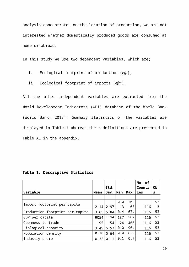
Table 1. Descriptive Statistics

Variable MeanStd.Dev. Min Max

No. ofCountries

Obs

Import footprint per capita 2.14 2.970.03

20.03 116

533

Production footprint per capita 3.65 5.84 0.47

67.39

116 533GDP per capita 9054 1194

6137 562

85116 53

3Openness to trade 95 54 24 460 116 533Biological capacity 3.49 6.57 0.0

290.54

116 533Population density 0.18

80.64 0.0

026.913

116 533Industry share 0.32 0.11 0.1

30.7

9116 53

320

Energy use per capita 2.46 2.65 0.01

16.87

116 533Stringency of environmental

regulation4.04 1.13 2.0

66.7

3116 53

3Enforcement of environmental regulations

3.83 1.03 1.83

6.34

116 533Note: See Table A1 for a detailed explanation and sources of all the

variables used in the analysis.

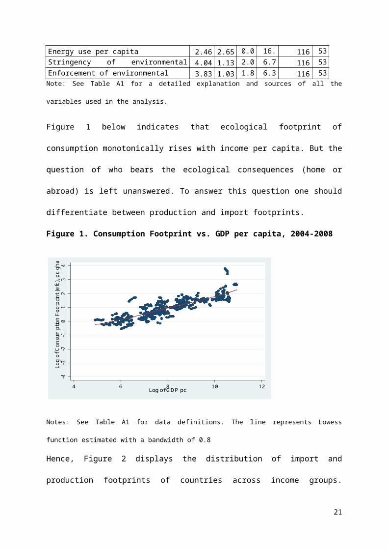
Figure 1 below indicates that ecological footprint of

consumption monotonically rises with income per capita. But the

question of who bears the ecological consequences (home or

abroad) is left unanswered. To answer this question one should

differentiate between production and import footprints.

Figure 1. Consumption Footprint vs. GDP per capita, 2004-2008

-10

12

34

-2-3

-4Lo

g of Con

sumption

Foo

tprin

t (efc), p

c gha

4 6 8 10 12Log of GDP pc

Notes: See Table A1 for data definitions. The line represents Lowess

function estimated with a bandwidth of 0.8

Hence, Figure 2 displays the distribution of import and

production footprints of countries across income groups.

21

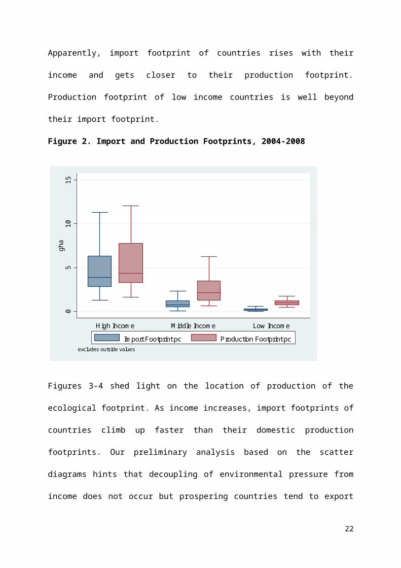
Apparently, import footprint of countries rises with their

income and gets closer to their production footprint.

Production footprint of low income countries is well beyond

their import footprint.

Figure 2. Import and Production Footprints, 2004-2008

05

1015

gha

High Incom e M iddle Incom e Low Incom e

excludes outside valuesIm port Footprint pc Production Footprint pc

Figures 3-4 shed light on the location of production of the

ecological footprint. As income increases, import footprints of

countries climb up faster than their domestic production

footprints. Our preliminary analysis based on the scatter

diagrams hints that decoupling of environmental pressure from

income does not occur but prospering countries tend to export

22

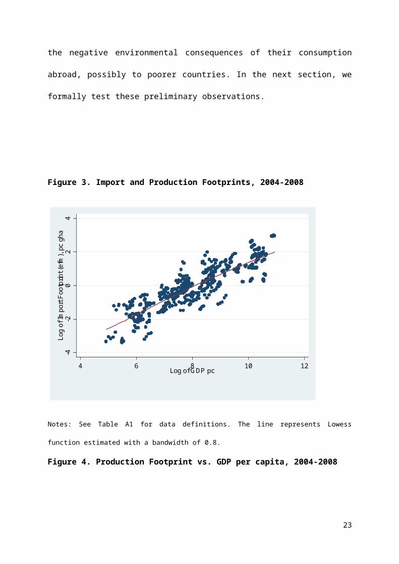
the negative environmental consequences of their consumption

abroad, possibly to poorer countries. In the next section, we

formally test these preliminary observations.

Figure 3. Import and Production Footprints, 2004-2008

-4-2

02

4Log of Im

port Footprint (efm), pc gha

4 6 8 10 12Log of G DP pc

Notes: See Table A1 for data definitions. The line represents Lowess

function estimated with a bandwidth of 0.8.

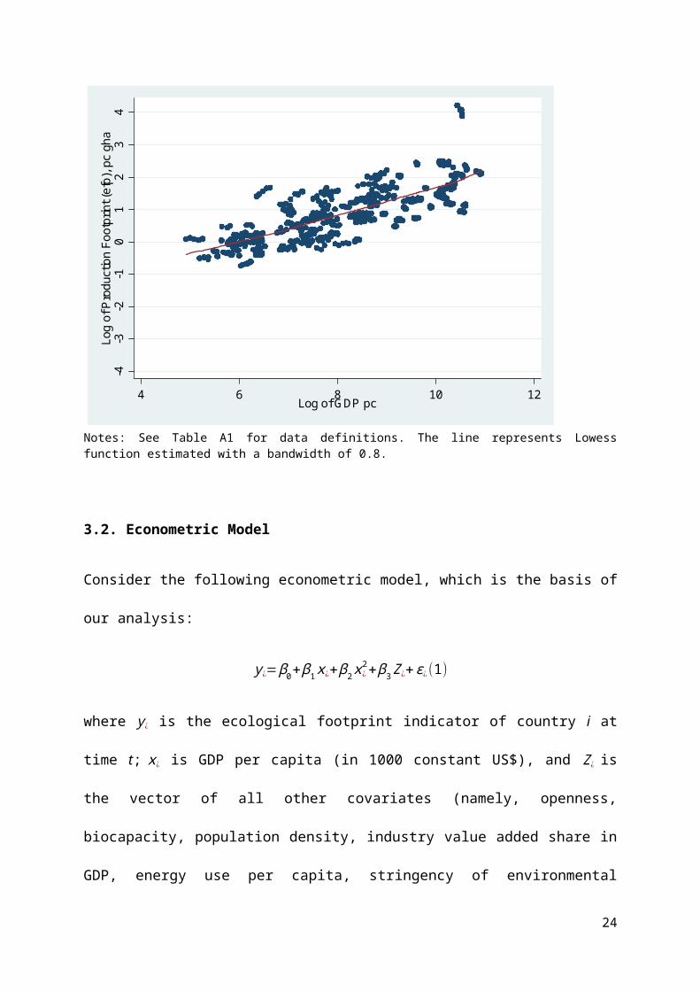
Figure 4. Production Footprint vs. GDP per capita, 2004-2008

23

-10

12

34

-2-3

-4Log of Production Footprint (efp), pc g

ha

4 6 8 10 12Log of G DP pc

Notes: See Table A1 for data definitions. The line represents Lowessfunction estimated with a bandwidth of 0.8.

3.2. Econometric Model

Consider the following econometric model, which is the basis of

our analysis:

y¿=β0+β1x¿+β2x¿2+β3Z¿+ε¿ (1)

where y¿ is the ecological footprint indicator of country i at

time t; x¿ is GDP per capita (in 1000 constant US$), and Z¿ is

the vector of all other covariates (namely, openness,

biocapacity, population density, industry value added share in

GDP, energy use per capita, stringency of environmental

24

regulation, and enforcement of environmental regulations)5 of

country i in year t. ε¿ is the error term, capturing all other

omitted factors with E(ε¿) = 0.

Equation 1 is estimated via the fixed effects panel data model

using the following dependent variables: production footprint

(efp) and import footprint (efm).

The possible outcomes can be listed as follows:

1. If β1> 0 and β2>0, there is a positive quadratic

relationship;

2. If β1> 0 and β2 is either insignificant or equal to zero,

there is a monotonically increasing relationship;

3. If β1< 0 and β2<0, there is a negative quadratic

relationship;

4. If β1< 0 and β2 is either insignificant or equal to zero,

there is a monotonically decreasing relationship;

5. If β1> 0 and β2< 0, there is an EKC-type (inverted U-type)

relationship;6

5 See Table 1 for the summary statistics and Table A1 for the description and units of both the dependent and independent variables employed in the analysis.6 The turning point for income per capita after which environmental quality improves is equal to−β1/2β2 .

25

6. If β1< 0 and β2> 0, there is a U-type relationship between

the relevant footprint indicator and income per capita.

In a panel data setting, one of the important issues that need

to be addressed is the problem of endogeneity between the

regressors and country specific effects. Due to the possible

correlation between the explanatory variables and the

individual effects in our model, we employ the fixed effects

model specification, which allows for endogeneity of all the

regressors with these country fixed effects (Baltagi, 2005:

19).

4. Results

Table 2 displays the regression results of the baseline and the

augmented (environmental regulation added) models. To begin

with, coefficients of per capita income and its square are all

significant and have the signs that confirm the EKC hypothesis.

As income per capita rises, footprint of import (efm) as well

as that of production (efp) first tend to increase. After a

certain threshold point for income, efp is expected to decrease.

That means the negative impact of economic growth on the

26

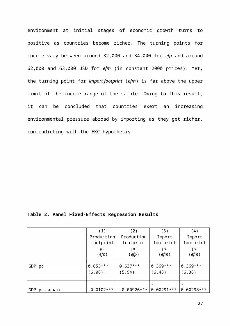
environment at initial stages of economic growth turns to

positive as countries become richer. The turning points for

income vary between around 32,000 and 34,000 for efp and around

62,000 and 63,000 USD for efm (in constant 2000 prices). Yet,

the turning point for import footprint (efm) is far above the upper

limit of the income range of the sample. Owing to this result,

it can be concluded that countries exert an increasing

environmental pressure abroad by importing as they get richer,

contradicting with the EKC hypothesis.

Table 2. Panel Fixed-Effects Regression Results

(1) (2) (3) (4)Productionfootprint

pc(efp)

Productionfootprint

pc(efp)

Importfootprint

pc(efm)

Importfootprint

pc(efm)

GDP pc 0.653*** 0.637*** 0.369*** 0.369***(6.08) (5.94) (6.48) (6.38)

GDP pc-square -0.0102*** -0.00926***-0.00291***

-0.00298***

27

(-6.15) (-5.45) (-3.31) (-3.26)

Openness -0.356 -0.171 0.447** 0.410**(-0.93) (-0.45) (2.20) (2.00)

Biocapacity 1.326*** 1.323*** -0.194* -0.194*(6.89) (6.97) (-1.90) (-1.90)

Population Density -3.20*** -3.67*** -0.369 -0.303(-3.05) (-3.52) (-0.66) (-0.54)

Industry 1.279 1.030 -0.211 -0.189(0.70) (0.57) (-0.22) (-0.20)

Enery Use pc -1.129*** -1.192*** 0.162*** 0.172***(-11.46) (-12.09) (3.10) (3.25)

Stringency of Env. Regulation 0.384** -0.0353

(2.35) (-0.40)

Enforcement of Env. Regulation -0.639*** 0.101

(-3.67) (1.08)

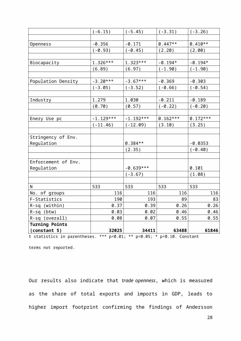
N 533 533 533 533No. of groups 116 116 116 116F-Statistics 190 193 89 83R-sq (within) 0.37 0.39 0.26 0.26R-sq (btw) 0.03 0.02 0.46 0.46R-sq (overall) 0.08 0.07 0.55 0.55Turning Points (constant $) 32025 34411 63488 61846t statistics in parentheses. *** p<0.01; ** p<0.05; * p<0.10. Constant

terms not reported.

Our results also indicate that trade openness, which is measured

as the share of total exports and imports in GDP, leads to

higher import footprint confirming the findings of Andersson

28

and Lindroth (2001). As expected, having higher biocapacity per

capita tends to increase footprint of production, whereas it

decreases import footprint since countries with abundant

biocapacity stocks can deplete their own resources and consume

their own biological stocks.

Denser population causes lower domestic production footprint.

It might be argued that, in densely populated regions, energy

is expected to be consumed more efficiently (thanks to e.g.

central heating and dense and highly connected transportation

networks which reduce the need for private transportation).

Another possible explanation is that, concentration of services

can be expected to be higher than manufacturing activity in

densely populated areas. Both effects may help to reduce

production footprint. Industry value added share in GDP, on the other

hand, appears to have no effect on efm or efp.

Higher energy use per capita induces lower production footprint and

higher import footprint. The latter result meets our

expectations in the sense that countries which are not

sufficiently endowed with energy resources need to import most

of their energy, which increases their import footprint.

29

Finally, we examine the implications of stringency of environmental

regulation and enforcement of environmental regulation on the footprint

creation location. The results indicate that footprint of

domestic production increases as regulation becomes more

stringent. On the other hand, as enforcement of regulations

becomes more rigorous, footprint of domestic production

decreases. Our findings are parallel to Heyes (2000), which

argues that incentives for non-compliance increase as

regulations become more stringent, which, in turn, creates the

necessity of stronger enforcement. Depending on the magnitudes

of estimated coefficients, one can see that negative

enforcement effect dominates positive stringency effect. Hence

we can conclude that environmental regulations do decrease

domestic production footprint. However, stringency or

enforcement of regulations has no significant effect on import

footprint. That is to say, domestic regulations do not

influence country decisions to import the environmentally

harmful products from abroad; but they do affect domestic

production characteristics. It is also noteworthy that income

turning points change significantly once environmental

regulation is accounted for. In the case of import footprint

30

threshold income drops from 63,488 USD down to around 61,846

USD, whereas in the case of production footprint, turning point

income per capita increases from 32,025 USD to 34,411 USD when

we include the stringency of environmental regulation and enforcement of

environmental regulation variables.

5. Conclusion and Discussion

Economic growth has been generally put forward as the key

panacea to environmental problems in the contemporary world

with reference to the improving environmental quality in some

countries thanks to higher access to cleaner technologies, more

efficient production systems and increased awareness of people

as they get richer. Rising awareness with income is also

expected to be translated into tightened environmental

regulation which helps to reduce the effect of income

generation on environment. The effect of GDP on environmental

quality after a certain level of income has been widely

investigated in the EKC literature. Yet, what the existing

studies fail to address is the question of who bears the

ecological consequences of affluence. Increased environmental

31

quality at home does not necessarily indicate a more

sustainable consumption pattern at home, since, thanks to

widening international trade, countries can choose to import

rather than produce domestically environmentally harmful

products. In this study, we aim to fill this gap in the

literature.

Controlling for country-fixed effects and several indicators

such as openness, biocapacity, etc., our results validate the

EKC hypothesis only for the relationship between income per

capita and ecological footprint of production. In the case of

footprint of imports, the estimated income turning points are

out of the income range of the sample. This supports our

hypothesis that as countries grow richer they tend to export

the ecological cost of their consumption to poorer economies.

We also investigate the implications of stringency and enforcement

of environmental regulation on the location of the environmental

pressure. The results reveal that more stringent regulation

leads to an increase in the footprint of domestic production.

Hence, stringer regulation seems to increase non-compliance and

aggravated the situation. However, if non-compliance behaviour

is to be avoided by tightened enforcement, domestic production

32

footprint decreases. On the other hand, this is not the case

for import footprint. We find that, domestic environmental

regulations do not bear any significant effect on footprint of

imports.

To sum up, given the diverging economic, environmental and

political characteristics of countries, economic growth in

itself is not sufficient to mitigate negative environmental

externalities. The significantly changed income turning points

show the importance of environmental regulation and its

enforcement along with economic growth. Our findings support

the view of Van Alstine and Neumayer (2010) that “grow now,

clean up later” message of standard EKC studies might be

misleading for developing and less developed countries given

the predictions that many countries will not reach EKC turning

points for decades to come. The finding that countries replace

domestic production of environmentally damaging goods by

imports as they get richer confirms our hypothesis that they

export the ecological cost of their consumption to poorer

economies. Hence, the answer to the question in the title of

this study is that income growth relocates ecological

footprint. Increasing volume of trade, in the absence of proper

33

institutional framework, would aggravate the situation under

the business-as-usual scenario. Reminding the latest report of

The Intergovernmental Panel on Climate Change (IPCC, 2013) on

the science of global warming, human activity and the

unquestioned fetishism of economic growth are to be blamed as

the primary causes of not only climate change, but also other

dimensions of environmental degradation that have been

scrutinized in the present study.

References

Al-mulali, U. and Tang, C.F. 2013. Investigating the validity

of pollution haven hypothesis in the gulf cooperation council

(GCC) countries. Energy Policy, 60: 813–819.

Al-mulali, U., Weng-Wai, C., Sheau-Ting, L., and Mohammed, A.H.

2015. Investigating the environmental Kuznets curve (EKC)

hypothesis by utilizing the ecological footprint as an

indicator of environmental degradation. Ecological Indicators,

48: 315–323

34

Andersen, R. 2008. Modern Methods for Robust Regression. Sage

University Paper Series on Quantitative Applications in the

Social Sciences, 07-152.

Andersson, J. O., Lindroth, M. 2001. Ecologically unsustainable

trade. Ecological Economics, Volume 37, Issue 1, 1 April 2001:

113-122.

Atici, C. 2009. Carbon Emissions in Central and Eastern Europe:

Environmental Kuznets Curve and Implications for Sustainable

Development. Sustainable Development, 17: 155–160.

Bagliani, M., Bravo, G., Dalmazzone, S. 2008. A consumption-

based approach to environmental Kuznets curves using the

ecological footprint indicator. Ecological Economics, 65(3):

650-661.

Baltagi, B. H., 2005. Econometric Analysis of Panel Data, 3rd

edition, John Wiley & Sons Ltd., West Sussex, England.

Berlik, M.M., Kittredge, D.B., Foster, D.R., 2002. The Illusion

of Preservation: A Global Environmental Argument for the Local

Production of Natural Resources. Harvard Forest Paper No. 26.

Harvard University, Petersham, MA.

35

Birdsall, N., Wheeler, D., 1993. Trade policy and industrial

pollution in Latin America: Where are the pollution havens?

Journal of Environment and Development 2 (1): 137–149.

Carson, R. T., 2010. The Environmental Kuznets Curve: Seeking

Empirical Regularity and Theoretical Structure. Review of

Environmental Economics and Policy, Association of

Environmental and Resource Economists, vol. 4(1): 3-23, Winter.

Caviglia-Harris J.L., Chambers D., Kahn J., 2009. Taking the

"U" out of Kuznets. Ecological Economics, 68 (4): 1149-1159.

Chen, D., Ma, X., Mu, H. and Li, P. 2010. The Inequality of

Natural Resources Consumption and Its Relationship with the

Social Development Level Based on the Ecological Footprint and

the HDI. Journal of Environmental Assessment Policy and

Management, 12 (1): 69–86.

Cheng, C. Lai, Y.B., 2012. Does a stricter enforcement policy

protect the environment? A political economy perspective.

Resource and Energy Economics, 34(4): 431-441.

Cole, M.A. 2004. Trade, the pollution haven hypothesis and

environmental Kuznets curve: examining the linkages. Ecological

Economics, 48 (1): 71–81.

36

Daly, H.E. 1993. The perils of free trade, Scientific American

Magazine, Vol. 269 No.5: 24–29.

Frankel, J. A. and Rose, A. K. 2005. Is Trade Good or Bad for

the Environment? Sorting Out the Causality. The Review of

Economics and Statistics, Vol. 87 No.1: 85-91.

Galli, A., Kitzes, J., Wermer, P., Wackernagel, M., Niccolucci,

V., Tiezzi, E., 2007. An exploration of the mathematics behind

the Ecological Footprint. International Journal of Ecodynamics

2 (4): 250–257.

Galli, A., Kitzes, J., Niccolucci, V., Wackernagel, M., Wada,

Y., and Marchettini, N. 2012. Assessing the global

environmental consequences of economic growth through the

Ecological Footprint: A focus on China and India. Ecological

Indicators, 17: 99–107.

Global Footprint Network, 2012. National Footprint Accounts,

2011 Edition. Available online at

http://www.footprintnetwork.org.

Global Footprint Network, 2010. Ecological Wealth of Nations,

Report published in April 2010 by Global Footprint Network,

Oakland, California, United States of America.

37

Grossman, G.M. and Krueger, A.B. 1991. Environmental Impacts of

North American Free Trade Agreement. NBER Working Paper Series

No: 3914.

Grossman, G. M., and Krueger, A. B. 1995. Economic Growth and

the Environment. Quarterly Journal of Economics, 110(2): 353-

377.

Gujarati, D. N., 1995. Basic Econometrics. Third Edition.

McGraw-Hill, Inc.

Heyes, A., 2000. Implementing environmental regulation:

enforcement and compliance. Journal of Regulatory Economics.,

17 (2):107–129.

Huber, P.J. 1973. Robust regression: Asymptotics, conjectures

and Monte Carlo. Annals of Statistics, 1: 799-821.

Intergovernmental Panel on Climate Change (IPCC). 2013.Climate

Change 2013: The Physical Science Basis. Working Group I

Contribution to the IPCC 5th Assessment Report - Changes to the

Underlying Scientific/Technical Assessment, (IPCC-XXVI/Doc.4),

27 September.

Jaffe, A.B., Peterson, S.R., Portney, P.R., Stavins, R.N. 1995.

Environmental regulation and the competitiveness of US38

manufacturing: what does the evidence tell us? Journal of

Economic Literature 33: 132– 163.

Janicke, M., Binder, M., Monch, H., 1997. ‘Dirty industries’:

patterns of change in industrial countries. Environmental and

Resource Economics, 9: 467– 491.

Kearsley, A. and Riddel, M. 2010. A further inquiry into the

Pollution Haven Hypothesis and the Environmental Kuznets Curve.

Ecological Economics, 69: 905–919

Lucas, R.E.B., Wheeler, D., Hettige, H., 1992. Economic

development, environmental regulation and the international

migration of toxic industrial pollution: 1960–88. In: Low, P.

(Ed.), International Trade and the Environment.World Bank

Discussion Paper No. 159.

Mani, M., Wheeler, D., 1998. In search of pollution havens?

Dirty industry in the world economy, 1960–1995. Journal of

Environment and Development 7 (3): 215– 247.

Mayer, A.L., Kauppi, P.E., Angelstam, P.K., Zhang, Y., Tikka,

P., 2005. Importing timber, exporting ecological impact.

Science 308: 359–360.

39

Mol, A. P. J. 1995. The Refinement of Production: Ecological

Modernization Theory and the Dutch Chemical Industry. Utrecht,

The Netherlands: Jan van Arkel/International Books.

Nordström, H., Vaughan, S. 1999. Trade and environment. In: WTO

Special Studies.

OECD, 2002. Indicators to Measure Decoupling of Environmental

Pressure from Economic Growth. Report on Sustainable

Development, 16 May, SG/SD(2002)1/FINAL.

Ozler, S. Ilgu, Obach, Brian, 2009. Capitalism, state economic

policy, and ecological footprint: an international comparative

analysis. Global Environmental Politics, 9: 79–108.

Peters, G.P., Minx, J.C., Weber, C.L., Edenhofer, O., 2011.

Growth in emission transfers via international trade from 1990

to 2008. Proceedings of the National Academy of Sciences of the

United States of America 108, 8903–8908.

Rivera, J. And Oh, C. H. 2013. Environmental Regulations and

Multinational Corporations’ Foreign Market Entry Investments.

The Policy Studies Journal, Vol. 41, No. 2.

Schütz, H., Moll, S., Bringezu, S., 2004. Globalisation and the

shifting environmental burden: material trade flows of the40

European Union. Wuppertal Papers No. 134e, Wuppertal Institute

für Klima, Wuppertal.

Saboori, B. and Soleymani, A. 2011. CO2 emissions, economic

growth and energy consumption in Iran: A co-integration

approach. International Journal of Environmental Sciences, Vol.

2, No. 1: 44-53.

Tobey, J., 1990. The effects of domestic environmental policies

on patterns of world trade: an empirical test. Kyklos 43 (2):

191– 209.

Van Alstine, James and Neumayer, Eric (2010) The environmental

Kuznets curve. in Gallagher, Kevin P., (ed.) Handbook on trade

and the environment. Edward Elgar, Cheltenham, UK: 49-59.

Wackernagel, M. and Rees, W.E., 1996. Our Ecological Footprint:

Reducing Human Impact on the Earth. New Society Publishers,

Gabriola Island.

Wang, Y., Kang, L., Wu, Xi., Xiao, Y. 2013. Estimating the

environmental Kuznets curve for ecological footprint at the

global level: A spatial econometric approach, Ecological

Indicators, 34(November): 15-21.

41

Weinzettel, J., Hertwich, E. A., Peters, G. P., Steen-Olsen,

K., Galli, A. 2013. Affluence drives the global displacement of

land use, Global Environmental Change 23: 433–438.

World Bank. 2013. World Development Indicators Online (WDI)

database (Accessed December 2013).

World Economic Forum. 2008. Executive Opinion Survey.

World Wildlife Fund for Nature, 2012. Türkiye’nin Ekolojik Ayak

İzi Raporu, WWF-Türkiye, İstanbul.

York, R., Rosa, E.A. and Dietz, T. 2004. The Ecological

Footprint Intensity of National Economies. Journal of

Industrial Ecology, 8(4): 139-154.

42

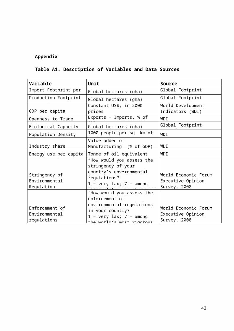
Appendix

Table A1. Description of Variables and Data Sources

Variable Unit SourceImport Footprint per capita

Global hectares (gha) Global Footprint Network, 2012Production Footprint

per capitaGlobal hectares (gha) Global Footprint

Network, 2012GDP per capita

Constant US$, in 2000 prices

World Development Indicators (WDI)

Openness to Trade Exports + Imports, % of GDP

WDIBiological Capacity Global hectares (gha) Global Footprint

Network, 2012Population Density 1000 people per sq. km of

land areaWDI

Industry shareValue added of Manufacturing (% of GDP) WDI

Energy use per capita Tonne of oil equivalent WDI

Stringency of Environmental Regulation

“How would you assess the stringency of your country’s environmental regulations?”1 = very lax; 7 = among the world’s most stringent

World Economic Forum Executive Opinion Survey, 2008

Enforcement of Environmental regulations

“How would you assess the enforcement of environmental regulations in your country?”1 = very lax; 7 = among the world’s most rigorous

World Economic Forum Executive Opinion Survey, 2008

43