This PDF is a selection from a published volume from the National Bureau of Economic Research Volume Title: Economic Aspects of Obesity Volume Author/Editor: Michael Grossman and Naci H. Mocan, editors Volume Publisher: University of Chicago Press Volume ISBN: 0-226-31009-4 ISBN13: 978-0-226-31009-1 Volume URL: http://www.nber.org/books/gros09-1 Conference Date: November 10-11, 2008 Publication Date: April 2011 Chapter Title: Does Health Insurance Make You Fat? Chapter Authors: Jay Bhattacharya, M. Kate Bundorf, Noemi Pace, Neeraj Sood Chapter URL: http://www.nber.org/chapters/c11825 Chapter pages in book: (35 - 64)

Welcome message from author
This document is posted to help you gain knowledge. Please leave a comment to let me know what you think about it! Share it to your friends and learn new things together.
Transcript
This PDF is a selection from a published volume from the National Bureau of Economic Research
Volume Title: Economic Aspects of Obesity
Volume Author/Editor: Michael Grossman and Naci H. Mocan, editors
Volume Publisher: University of Chicago Press
Volume ISBN: 0-226-31009-4ISBN13: 978-0-226-31009-1
Volume URL: http://www.nber.org/books/gros09-1
Conference Date: November 10-11, 2008
Publication Date: April 2011
Chapter Title: Does Health Insurance Make You Fat?
Chapter Authors: Jay Bhattacharya, M. Kate Bundorf, Noemi Pace, Neeraj Sood
Chapter URL: http://www.nber.org/chapters/c11825
Chapter pages in book: (35 - 64)
35
2Does Health Insurance Make You Fat?
Jay Bhattacharya, M. Kate Bundorf, Noemi Pace, and Neeraj Sood
2.1 Introduction
Adult obesity is a thorny problem. Several studies document rising obe-sity prevalence in the United States (See Mokdad et al. 1999; Mokdad et al. 2003). Economists have argued that the primary cause of increasing obe-sity prevalence are: (a) a falling relative price of food; (b) a technologically induced shift away from physically demanding work; and (c) a decline in time spent on food production at home (see Lakdawalla and Philipson 2002; Cut-ler, Glaeser, and Shapiro 2003; and Anderson, Butcher, and Levine 2003).1 As most view these fundamental changes in the economy as desirable and would not want to undo them, developing public policy to address the root causes of rising obesity prevalence is difficult, if not entirely problematic.
Jay Bhattacharya is associate professor of medicine and a core faculty member of the Center for Health Policy/ Center for Primary Care and Outcomes Research (CHP/ PCOR) at Stanford University, and a research associate of the National Bureau of Economic Research. M. Kate Bundorf is assistant professor of Health Research and Policy and fellow of the Center for Health Policy/ Center for Primary Care and Outcomes Research (CHP/ PCOR) at Stanford University, and a faculty research fellow of the National Bureau of Economic Research. Noemi Pace is assistant professor of economics at Ca’ Foscari University of Venice. Neeraj Sood is associate professor of Clinical Pharmacy and Pharmaceutical Economics and Policy at the University of Southern California School of Pharmacy, and a faculty research fellow of the National Bureau of Economic Research.
We thank Michael Grossman and the participants at the NBER Conference on the Econom-ics of Obesity for helpful comments. Bhattacharya, Sood, and Bundorf thank the National Institute of Aging for fi nancial support on this project.
1. There are, of course, many other noneconomic determinants of body weight, including genetic predispositions to obesity and nonrational impulses (such as myopic decision making and lack of self- control) that prevent optimal body weight control. These are unlikely explana-tions for the observed trends in body weight, even if they help explain baseline levels. There is certainly no evidence that we are more irrational or have different genes than our parents or grandparents.
36 Jay Bhattacharya, M. Kate Bundorf, Noemi Pace, and Neeraj Sood
Nevertheless, the health care and other costs associated with obesity are enormous. For example, Wolf and Colditz (1994) estimate that over $68 bil-lion are lost annually in increased health care costs and job absenteeism as a result of obesity in the United States. The morbidity and accounting costs associated with obesity have led public health experts (such as Nestle 2003; Brownell and Horgen 2003; and Sturm 2002) to advocate vigorous public intervention, including regulation of fast- food establishments and taxes on nutritionally questionable foods.
The economic justifi cation for these sorts of policy interventions, such as taxes on food, favored by some of these authors, rests on the idea that when one person becomes obese, many other people pay the cost. In economic jargon, there are negative externalities from body weight decisions that lead to obesity. If external costs are high, then public welfare can be improved by interventions that change the incentives adults face when making decisions about body weight. If external costs are small, then adults pay fully for their body weight decisions and public interventions aimed at decreasing body weight can play only a limited role in improving public welfare.2
The main mechanism by which obesity imposes external costs is through pooled health insurance. In a health insurance pool with inadequately risk- adjusted premiums, one person’s increase in body weight really is everyone else’s business, since obesity often leads to higher medical expenditures. In this chapter, we describe a model of this negative obesity externality associ-ated with health insurance.3 The main insight of this model is that measur-ing the obesity externality involves more than just measuring the subsidy to obese individuals induced by health insurance. The welfare loss due to the obesity externality depends upon both the size of the subsidy and upon the extent to which body weight decisions are distorted on the margin by the subsidy—that is, does coverage with pooled health insurance cause enrollees to gain weight? If the answer is no, and there is no moral hazard of this sort caused by insurance coverage, then the subsidy induced by one person’s obesity would simply represent a transfer from the thinner individuals in his insurance pool to the obese person, with no net effect on social welfare.
Despite the importance of this parameter—the health insurance elasticity of body weight—to the welfare economics of obesity, there has been scant work in the economics literature on the topic.4 The one exception is a paper by Rashad and Markowitz (2010) who fi nd a zero elasticity of insurance coverage on body weight or obesity rates. These authors rely on the size of a fi rm where an individual works as an instrument for insurance coverage in their body weight regressions. We extend this work along three dimen-
2. Cawley (2004) provides a detailed discussion of possible market failures related to obe-sity.
3. See Bhattacharya and Sood (2007) for a full description of this model.4. In a related study, Dave and Kaestner (2009) analyze the effect of insurance on smoking,
drinking, and exercise in the elderly population. They fi nd that obtaining health insurance reduces prevention and increases unhealthy behaviors among elderly men.
Does Health Insurance Make You Fat? 37
sions. First, we measure separate elasticities for the extensive margin (people gaining or losing insurance altogether) and the intensive margin (insurance becoming more generous). In principle, these elasticities may be different, and as we show in the concluding section of the chapter, they have different policy implications. Second, we distinguish different elasticities for public and private insurance coverage for our estimates of the elasticity along the extensive margin. Finally, we adopt econometric methods that account for the discrete nature of the insurance coverage variable.
2.2 Background
Not surprisingly, expected health care expenditures are higher for obese individuals than for normal weight individuals. A large number of stud-ies document this fact. The vast majority of these studies use convenience samples consisting of individuals from a single employer or a single insurer (Elmer et al. 2004; Bertakis and Azari 2005; Burton et al. 1998; Raebel et al. 2004). There are also studies of obesity- related medical expenditure differences in an international setting. Both Sander and Bergemann (2003), in a German setting, and Katzmarzyk and Janssen (2004), in a Canadian setting, fi nd higher medical expenditures for obese people.
There are a few studies that use nationally representative data. Finkel-stein, Fiebelkorn, and Wang (2003) use data from the linked National Health Interview Survey (NHIS) and Medical Expenditure Panel Survey (MEPS). They estimate that annual medical expenditures are $732 higher for obese than normal weight individuals. From an accounting viewpoint, approxi-mately half of the estimated $78.5 billion in medical care spending in 1998 attributable to excess body weight was fi nanced through private insurance (38 percent) and patient out- of- pocket payments (14 percent). Sturm (2002), using data from the Health Care for Communities (HCC) survey, fi nds that obese individuals spend $395 per year more than nonobese individuals on medical care. Thorpe et al. (2004) also use MEPS data, but they are inter-ested in how much of the $1,100 increase between 1987 and 2000 in per- capita medical expenditures is attributable to obesity. Using a regression model to calculate what per- capita medical expenditures would have been had 1987 obesity levels persisted to 2000, they conclude that about $300 of the $1,100 increase is due to the rise in obesity prevalence.
This is a large literature, which space constraints prevent us from sur-veying in more detail. The many studies that we do not discuss here vary considerably in generality—some examine data from a single company or from a single insurance source—though they all reach the same qualitative conclusion that obesity is associated with higher medical care costs.5
5. Some of the studies we reviewed, but arbitrarily do not discuss here, include Bungam et al. (2003); Musich et al. (2004); Quesenberry Jr., Caan, and Jacobson (1998); Thompson et al. (2001); and Wang et al. (2003).
38 Jay Bhattacharya, M. Kate Bundorf, Noemi Pace, and Neeraj Sood
2.2.1 External Costs of Obesity Associated with Health Insurance
Despite the extensive literature on medical expenditure differences, very few studies attempt to estimate the degree to which health insurance cover-age leads to subsidies for the obese. Some studies have attempted to esti-mate how much of obesity- related medical costs are subsidized by public insurance. Finkelstein, Ruhm, and Kosa (2005), in a literature review of the causes and consequences of obesity, estimate that “the government fi nances roughly half the total annual medical costs attributable to obesity. As a result, the average taxpayer spends approximately $175 per year to fi nance obesity related medical expenditures among Medicare and Medicaid recipi-ents” (248). To arrive at this conclusion, they rely on a study by Finkelstein, Fiebelkorn, and Wang (2004), who calculate state and federal level estimates of Medicare and Medicaid expenditures attributable to obesity. Another study, conducted by Daviglus et al. (2004), links together data from a sample of Chicago- area workers in the labor force between 1967 to 1973, to Medi-care claims records from the 1990s. They estimate substantial obesity- related differences in Medicare expenditures. For example, women workers who were obese between 1967 and 1973 spent $176,947 in the 1990s on Medicare, while analogous nonobese, nonoverweight female workers spent $100,431 in undiscounted costs. Obese male workers spent $125,470, while nonobese, nonoverweight male workers spent $76,866.
However, estimating how much of obesity- related medical costs are fi nanced by public insurance is merely an accounting exercise and not suf-fi cient for calculating the true economic subsidy for obesity. Conceptually, calculating the size of the subsidy also requires estimating payments by obese and nonobese individuals for enrolling in health insurance in addi-tion to the expected benefi ts of enrollment. Roughly speaking, obese and nonobese people alike pay for Medicare when they are under sixty- fi ve and spend (receive benefi ts) when they are older.6 Since obese people work, earn, are taxed, and die at different rates than nonobese people, looking at Medi-care expenditure differences alone will paint a misleading picture of the Medicare subsidy for the obese.
Calculating the obesity subsidy induced by private insurance also requires estimating both payments for health insurance and medical expenditures. Since private insurance is typically provided in an employment setting, it is not enough to look at premiums for health insurance paid by employers and employees.7 The key question is whether employers adjust the cash wages of obese workers with health insurance in order to account for the higher cost
6. For example, McClellan and Skinner (1999, 2006) and Bhattacharya and Lakdawalla (2006), in estimating Medicare progressivity, estimate lifetime profi les of tax receipts for Medi-care as well as Medicare expenditures.
7. For employees enrolling in the same insurance plan, premiums do not depend upon body weight (see Keenan et al. 2001), so in that case, there are no obesity- related payment differen-
Does Health Insurance Make You Fat? 39
of insuring these workers. Although theory predicts that employers would have incentives to do so (Rosen 1986), in practice, it is not clear that they would be able to make these adjustments.8 According to Gruber (2000), “. . . the problems of preference revelation in this context are daunting; it is difficult in reality to see how fi rms could appropriately set worker specifi c compensating differentials” (656).
As is the case with Medicare, however, there is very little research on obesity- related payment differences in a private insurance setting. An impor-tant exception is Bhattacharya and Bundorf (2009), who fi nd some evidence that obese workers receive lower pay than nonobese workers primarily at fi rms that provide health insurance.
In related work, Keeler et al. (1989) and Manning et al. (1991), using data from the RAND Health Insurance Experiment (RAND HIE) and from the National Health Interview Survey (NHIS), report estimates of lifetime medical costs attributable to physical inactivity (rather than obesity): “At a 5 percent rate of discount, the lifetime subsidy from others to those with a sedentary life style is $1,900” (Keeler er al. 1989). Though they label this estimate the “external cost of physical inactivity,” like the rest of the lit-erature they focus on physical inactivity- related medical expenditure differ-ences, while ignoring payment differences that occur outside experimental settings in their calculation of the subsidy.
2.3 A Model of the Social Costs of Obesity
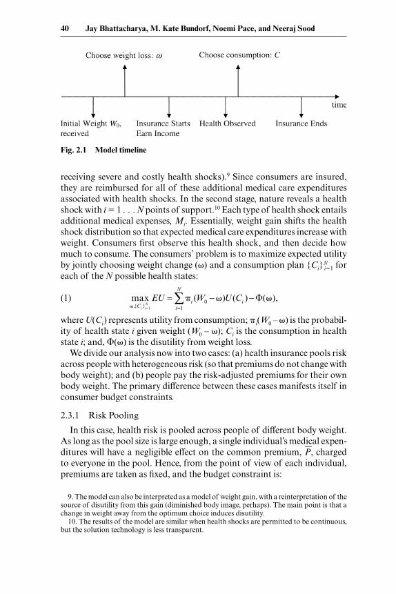
The timeline in fi gure 2.1 illustrates the basic setup of the model. Each consumer starts with an initial endowment of weight W0. This endowment might be seen as refl ecting the consumer’s genetic propensity to be over-weight or obese, and in any case it cannot be chosen by the consumer. In the fi rst stage, consumers decide how much weight to lose, �. Weight loss (exercising, dieting) gives consumers some disutility but has two associated benefi ts: (a) it increases productivity, consequently raising consumer income and (b) it improves health (more precisely, it decreases the probability of
ces. However, when employers offer multiple health plans, obese workers may tend to select into a different set of plans than their thinner colleagues. In that case, premiums may differ.
8. The literature on medical expenditure- associated obesity costs has a parallel and often intersecting literature on the labor market productivity costs associated with obesity (often these latter costs are called “indirect” costs of obesity). The theory of compensating wage differentials has important implications for whether these labor market costs are external; that is, whether obese individuals pay for lower productivity levels (such as through more sick days) associated with their body weight, or someone else pays. This theory suggests that obese workers will pay for lower productivity through reduced wages. The economics literature on obesity- related wage differences—for example, Register and Williams (1990), Pagan and Davila (1997), and Cawley (2000)—unanimously fi nds that obese workers earn lower wages than their thinner colleagues, and that these differences are equal to or greater than the wage differences that would arise from measurable productivity differences. Hence, both theory and evidence suggest that these “indirect” costs of obesity are not external.
40 Jay Bhattacharya, M. Kate Bundorf, Noemi Pace, and Neeraj Sood
receiving severe and costly health shocks).9 Since consumers are insured, they are reimbursed for all of these additional medical care expenditures associated with health shocks. In the second stage, nature reveals a health shock with i � 1 . . . N points of support.10 Each type of health shock entails additional medical expenses, Mi. Essentially, weight gain shifts the health shock distribution so that expected medical care expenditures increase with weight. Consumers fi rst observe this health shock, and then decide how much to consume. The consumers’ problem is to maximize expected utility by jointly choosing weight change (�) and a consumption plan {Ci}
Ni�1 for
each of the N possible health states:
(1) max
�,{Ci }i =1N
EU = �ii=1
N
∑ (W0 − �)U (Ci ) − �(�),
where U(Ci) represents utility from consumption; �i(W0 – �) is the probabil-ity of health state i given weight (W0 – �); Ci is the consumption in health state i; and, �(�) is the disutility from weight loss.
We divide our analysis now into two cases: (a) health insurance pools risk across people with heterogeneous risk (so that premiums do not change with body weight); and (b) people pay the risk- adjusted premiums for their own body weight. The primary difference between these cases manifests itself in consumer budget constraints.
2.3.1 Risk Pooling
In this case, health risk is pooled across people of different body weight. As long as the pool size is large enough, a single individual’s medical expen-ditures will have a negligible effect on the common premium, P�, charged to everyone in the pool. Hence, from the point of view of each individual, premiums are taken as fi xed, and the budget constraint is:
Fig. 2.1 Model timeline
9. The model can also be interpreted as a model of weight gain, with a reinterpretation of the source of disutility from this gain (diminished body image, perhaps). The main point is that a change in weight away from the optimum choice induces disutility.
10. The results of the model are similar when health shocks are permitted to be continuous, but the solution technology is less transparent.
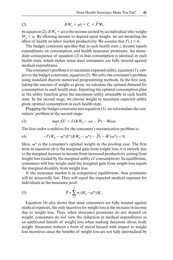
Does Health Insurance Make You Fat? 41
(2) I(W0 � �) � Ci � P� �i.
In equation (2), I(W0 � �) is the income earned by an individual who weighs W0 � �. By allowing income to depend upon weight, we are modeling the effect of health on labor market productivity. We assume that I�(.) 0.
The budget constraint specifi es that in each health state i, income equals expenditures on consumption and health insurance premiums. An imme-diate consequence of equation (2) is that consumption is identical in each health state, which makes sense since consumers are fully insured against medical expenditures.
The consumer’s problem is to maximize expected utility, equation (1), sub-ject to the budget constraint, equation (2). We solve the consumer’s problem using standard discrete numerical programming methods. In the fi rst step, taking the amount of weight as given, we calculate the optimal demand for consumption in each health state. Inputting the optimal consumption plan in the utility function gives the maximum utility attainable in each health state. In the second stage, we choose weight to maximize expected utility given optimal consumption in each health state.
Plugging the budget constraint into equation (1), we reformulate the con-sumers’ problem in the second stage:
(3) max�
EU � U(I(W0 �) P�) �(�).
The fi rst- order condition for the consumer’s maximization problem is:
(4) I�(W0 �∗)U�(I(W0 �∗) P�) ��(�∗) � 0.
Here, �∗ is the consumer’s optimal weight in the pooling case. The fi rst term in equation (4) is the marginal gain from weight loss; it is entirely due to the marginal increase in income from increased productivity arising from weight loss (scaled by the marginal utility of consumption). In equilibrium, consumers will lose weight until the marginal gain from weight loss equals the marginal disutility from weight loss.
If the insurance market is in competitive equilibrium, then premiums will be actuarially fair. They will equal the expected medical expenses for individuals in the insurance pool:
(5) P = �i
i=1
N
∑ (W0 − �*)Mi .
Equation (4) also shows that since consumers are fully insured against medical expenses, the only incentive for weight loss is the increase in income due to weight loss. Thus, when insurance premiums do not depend on weight, consumers do not view the reduction in medical expenditures as an additional benefi t of weight loss when making decisions about body weight. Insurance induces a form of moral hazard with respect to weight loss incentives since the benefi ts of weight loss are not fully internalized by
42 Jay Bhattacharya, M. Kate Bundorf, Noemi Pace, and Neeraj Sood
the consumer. As a consequence, weight loss creates a positive externality for everyone else in the insurance pool, since it lowers their health insurance pre-miums.11 Because this benefi t is not fully captured by the consumer losing the weight, insured people will tend to lose less weight than would be optimal. By contrast, the productivity benefi ts of weight loss are fully internalized as changes in productivity lead to an increase in consumer income.
2.3.2 Risk- Adjusted Insurance
We now turn to the case where health insurance premiums adjust to refl ect the weight choice of consumers. In contrast to the previous case, where the premium is taken as fi xed, consumers now face a risk- adjusted schedule of health insurance premiums that depends upon their own body weight. In the context of employer provided insurance, this could be achieved by wage reductions for obese employees, or simply by offering premium rebates to individuals who lose weight. In this case, the budget constraint is given by:
(6) I(W0 �) � Ci � P(W0 �) �i.
Here, P(W0 – �) is the health insurance premium for an individual who weighs W0 – �. Again, if the insurance market is competitive, premiums will be actuarially fair. Hence, they will be an increasing function of weight, refl ecting the increase in expected medical expenses:
(7) P(W0 �) � � �ii=1
N
∑ (W0 − �)Mi�.
The consumers’ problem in this case can be reformulated as:
(8) max
�EU � U(I(W0 �) P(W0 �)) �(�).
The fi rst- order condition for the consumer’s maximization problem is:
(9) [I�(W0 �∗∗) P�(W0 �∗∗)]U�(I(W0 �∗∗) P(W0 �∗∗))
��(�∗∗) � 0.
Here, �∗∗ is the consumer’s optimal weight in the risk- adjusted case. Clearly, equation (9) is necessary for �∗∗ to be individually optimal, but whether it is also socially optimal depends upon what is meant by social opti-mality. Suppose EU is the expected utility of the representative consumer in the economy, and all individuals start with the same initial weight, W0. In that (unrealistic) case, �∗∗ can be said to be socially optimal, since the full social costs of body weight decisions are internalized. In the appendix, we consider a more realistic case where W0 differs across individuals in the
11. This argument is developed in more detail in the appendix.
Does Health Insurance Make You Fat? 43
population. We show that, aside from transfers that do not depend upon fi nal weight, W0 – �∗∗, equation (9) is a necessary condition for the social optimum.
It is instructive to compare the fi rst order condition in equation (9) with the analogous condition in equation (4), when there was a single risk pool. Both equations have a single term refl ecting the marginal costs of weight loss: ��(.). However, equation (9) has two terms, I�(.) and P�(.), refl ecting the marginal benefi t of weight loss accruing from an increase in productivity and a decrease in the health insurance premium. By contrast, equation (4) has only a single term refl ecting the marginal productivity benefi t of weight loss: I�(.). Thus, when premiums refl ect individual health risk, consumers have two incentives for weight loss—productivity gains and lower health insurance premiums. In this case, there is no moral hazard induced by health insurance and consumer body weight decisions.
2.3.3 Deadweight Loss From the Obesity Externality
In this section, we show that the size of the loss in social welfare from the obesity externality under- pooled premiums depends upon both the fact that expected health expenditures are higher for the obese, and also upon how responsive people would be in their weight loss decisions to a switch from pooled to risk- adjusted premiums. This calculation is important because, while there is a lot of empirical evidence that obese people are more likely to have higher medical care expenditures than nonobese people, there is no empirical evidence on whether pooled insurance causes obesity or weight gain. Whether the rise in obesity prevalence is a public health crisis, or merely a private crisis for many people, depends on the evidence on both quantities.
We start with the expression for expected utility, evaluated at the optimum under risk- adjusted insurance:
(10) EU(�∗∗) � U(I(W0 �∗∗) P(W0 �∗∗)) �(�∗∗).
We have imposed the condition that consumption does not vary with health outcome since consumers are fully insured under both cases.
Next, we consider a fi rst- order Taylor series approximation of equation (10) around �∗, which is optimal weight loss under pooled insurance:
(11) EU(�∗∗) ≈ EU(�∗) � ∂EU�
∂� |�∗ (�∗∗ �∗).
The deadweight loss (DWL) from the obesity externality is the change in expected utility resulting from pooling. Equation (11) suggests an approxi-mation to this quantity:
(12) DWL � EU(�∗∗) EU(�∗) ≈ ∂EU�
∂� |�∗ ��.
44 Jay Bhattacharya, M. Kate Bundorf, Noemi Pace, and Neeraj Sood
Here, �� � �∗∗ – �∗ is the difference between optimal weight under risk- adjusted and pooled risk cases. Since weight is socially optimal in the risk- adjusted case, �� also refl ects the degree to which weight choice differs from socially optimal when pooling pertains.
Using a fi rst- order Taylor series approximation, the dead weight loss (DWL) in expected utility terms due to the obesity externality is:
(13) DWL ≈ {U�(I(W0 �∗) P(W0 �∗))
[I�(W0 �∗) � P�(W0 �∗)] ��(�∗)}��.
Substituting the fi rst order condition in equation (4) in equation (13) yields a simple expression for the dead weight loss from the obesity externality:
(14) DWL ≈ U�(.)P�(W0 �∗)��.
Equation (14) shows that the deadweight loss is proportional to two cru-cial factors: the extent to which body weight deviates from the optimal due to pooled health insurance when individuals do not bear the full medical care costs of obesity, ��, and the responsiveness of medical care expenditures to changes in weight, P�(W0 – �∗). The dead weight loss from the obesity externality is zero if individual weight choice does not respond to subsidies for obesity, or if medical expenditures do not change with body weight.
While several estimates of P�(W0 – �∗) are available from the public health and economics literatures, there is no work that quantifi es ��. To estimate ��, ideally, we would like to know: (a) body weight under pooled insurance when the consumer is shielded from the medical care costs of obesity and (b) under risk- adjusted premiums when the individual faces the full medical care costs of obesity. To answer whether obesity creates a negative exter-nality and lost social welfare through the health insurance mechanism, we need to know whether risk- rating insurance premiums affects body weight. Unfortunately, there are no real world data that we are aware of that would permit us to ascertain the effect of risk rating on body weight.
Instead, we aim at answering a related question—whether insurance cov-erage expansions along both extensive and intensive margins cause body weight to change. It is our conjecture that if insurance coverage does not infl uence body weight choices, it is unlikely that risk rating would infl u-ence body weight choices. Conversely, if health insurance expansion (along either intensive or extensive margins) does infl uence body weight, it is likely, depending on the mechanism by which risk rating is implemented, that risk rating would infl uence body weight. We start with an empirical consider-ation of the intensive margin—expansions in health insurance generosity. Next, we examine the effect of insurance status on the extensive margin; that is, whether the uninsured, who face the full medical care costs of obesity, weigh less than the insured.
Does Health Insurance Make You Fat? 45
2.4 The Intensive Margin: Increasing Generosity of Coverage
Using data from the RAND Health Insurance Experiment (HIE), we are able to examine the effect of health insurance on body weight when people are randomly assigned to different levels of insurance coverage (the intensive margin). In the HIE, which was conducted in six areas of the country during the late 1970s and early 1908s, approximately 2,000 nonelderly families were assigned to differing levels of insurance coverage.12 The purpose of the HIE was to determine the effects of patient cost sharing on medical care utiliza-tion and health. The participants were assigned to different fee- for- service plans that varied along two dimensions: the coinsurance rate (the fraction of billed charges paid by patients), and the maximum dollar expenditure (the maximum amount a family would spend on covered expenditures during a twelve- month period). The coverage was comprehensive in the sense that it included nearly all types of medical care. Participants remained enrolled in their assigned plan and were followed for either three (70 percent) or fi ve years.
The plans were characterized by four different coinsurance percent-ages—0 (often referred to as “free care”), 25 percent, 50 percent, and 95 per-cent—and three levels of maximum out- of- pocket spending—5 percent, 10 percent, and 15 percent of family income up to a maximum of $1,000. In one plan, the maximum dollar expenditure (MDE)—also known as maxi-mum out- of- pocket expenditures—was set at $150 per individual, and $450 per family (often referred to as the “individual deductible plan”).13 In this plan, the coinsurance rate was 95 percent. In our empirical work, we cat-egorize plans based on their coinsurance rate and control for the MDE.14 We categorize the individual deductible plan separately due to the more complicated structure of the MDE.
In order to minimize participation bias, the investigators offered a partici-pation incentive. The participation incentive for a given family was defi ned as “the maximum loss risked by changing to the experimental plan from existing coverage,” and was intended to ensure that families were equally likely to participate independent of their prior health insurance status and the plan to which they were assigned.
The study collected data on demographic and socioeconomic character-
12. This description of the HIE is based on information from Newhouse and the Insurance Experiment Group, 1993.
13. The HIE also included an analysis of the effects of enrolling in an HMO on the study outcomes. Because it is difficult to measure the generosity of a health maintenance organization (HMO) relative to a fee- for- service (FFS) plan, we drop these enrollees from the analysis.
14. The coinsurance rate was constant across different types of services with one exception. In one plan, the coinsurance rate was 25 percent for all services except outpatient mental health and dental, which had a 50 percent coinsurance rate. We include this plan in the 25 percent coinsurance rate group.
46 Jay Bhattacharya, M. Kate Bundorf, Noemi Pace, and Neeraj Sood
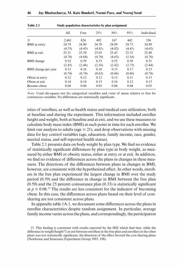
istics of enrollees, as well as health status and medical care utilization, both at baseline and during the experiment. This information included enrollee height and weight, both at baseline and at exit, and we use these measures to calculate body mass index (BMI) at each point in time for each enrollee. We limit our analysis to adults (age � 21), and drop observations with missing data for key control variables (age, education, family income, race, gender, marital status, and self- reported health status).
Table 2.1 presents data on body weight by plan type. We fi nd no evidence of statistically signifi cant differences by plan type in body weight, as mea-sured by either BMI or obesity status, either at entry or at exit. In addition, we fi nd no evidence of differences across the plans in changes in these mea-sures. The directions of the differences between plans in changes in BMI, however, are consistent with the hypothesized effect. In other words, enroll-ees in the free plan experienced the largest change in BMI over the study period (0.59) and the difference in change in BMI between the free plan (0.59) and the 25 percent coinsurance plan (0.33) is statistically signifi cant at p � 0.06.15 The results are less consistent for the indicator of becoming obese. In this case, the differences across plans based on their level of cost- sharing are not consistent across plans.
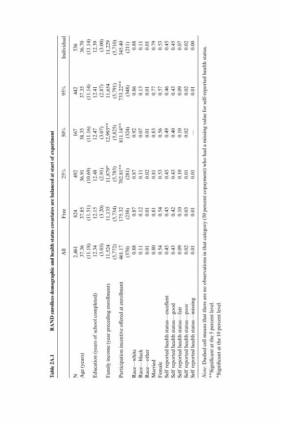
In appendix table 1A.1, we document some differences across the plans in enrollee characteristics despite random assignment. In particular, average family income varies across the plans, and correspondingly, the participation
Table 2.1 Study population characteristics by plan assignment
All Free 25% 50% 95% Individual
N 2,461 824 492 167 442 536BMI at entry 24.79 24.80 24.70 24.89 24.73 24.89
(4.53) (4.45) (4.81) (4.02) (4.41) (4.63)BMI at exit 25.31 25.39 25.03 25.43 25.31 25.40
(4.78) (4.64) (4.76) (4.63) (5.16) (4.76)BMI change 0.52 0.59 0.33 0.55 0.58 0.51
(2.45) (2.46) (2.16) (2.42) (2.75) (2.44)BMI change per year 0.15 0.16 0.10 0.15 0.17 0.15
(0.74) (0.74) (0.62) (0.66) (0.86) (0.74)Obese at entry 0.12 0.12 0.12 0.13 0.11 0.13Obese at exit 0.14 0.14 0.13 0.16 0.12 0.15Became obese 0.04 0.04 0.03 0.06 0.04 0.05
Note: Used chi- square test for categorical variables and t- test of mean relative to free for continuous variables. No differences are statistically signifi cant.
15. This fi nding is consistent with results reported by the HIE which fi nd that, while the difference in weight/ height^2 at exit between enrollees in the free plan and enrollees in the other plans was not statistically signifi cant, the direction of the effect favored the cost sharing plans (Newhouse and Insurance Experiment Group 1993, 198).
Does Health Insurance Make You Fat? 47
incentive as well. In addition, enrollee assignment to plans is not balanced by site.
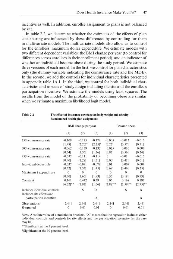
In table 2.2, we determine whether the estimates of the effects of plan cost- sharing are infl uenced by these differences by controlling for them in multivariate models. The multivariate models also allow us to control for the enrollees’ maximum dollar expenditure. We estimate models with two different dependent variables: the BMI change per year (to control for differences across enrollees in their enrollment period), and an indicator of whether an individual became obese during the study period. We estimate three versions of each model. In the fi rst, we control for plan characteristics only (the dummy variable indicating the coinsurance rate and the MDE). In the second, we add the controls for individual characteristics presented in appendix table 1A.1. In the third, we control for both individual char-acteristics and aspects of study design including the site and the enrollee’s participation incentive. We estimate the models using least squares. The results from the model of the probability of becoming obese are similar when we estimate a maximum likelihood logit model.
Table 2.2 The effect of insurance coverage on body weight and obesity—Randomized health plan assignment
BMI change per year Became obese
(1) (2) (3) (1) (2) (3)
25% coinsurance rate –0.109 –0.175 –0.179 –0.005 –0.012 –0.016[1.48] [2.20]∗ [2.25]∗ [0.23] [0.57] [0.71]
50% coinsurance rate –0.062 –0.139 –0.132 0.025 0.016 0.007[0.64] [1.36] [1.26] [0.92] [0.56] [0.24]
95% coinsurance rate –0.032 –0.111 –0.114 0 –0.01 –0.015[0.40] [1.28] [1.31] [0.00] [0.41] [0.61]
Individual deductible –0.037 –0.071 –0.079 0.01 0.007 0.004[0.72] [1.33] [1.45] [0.68] [0.46] [0.25]
Maximum $ expenditure 0 0 0 0 0 0[0.70] [1.65] [1.93] [0.35] [0.18] [0.73]
Constant 0.161 0.442 0.39 0.051 0.168 0.197[6.32]∗∗ [1.92] [1.66] [2.88]∗∗ [2.59]∗∗ [2.95]∗∗
Includes individual controls X X X XIncludes site effects and participation incentive X X
Observations 2,441 2,441 2,441 2,441 2,441 2,441R- squared 0 0.01 0.01 0 0.01 0.01
Note: Absolute value of t statistics in brackets. “X” means that the regression includes either individual controls and controls for site effects and the participation incentive (as the case may be).∗∗Signifi cant at the 5 percent level.∗Signifi cant at the 10 percent level.
48 Jay Bhattacharya, M. Kate Bundorf, Noemi Pace, and Neeraj Sood
The results from the multivariate models are substantively similar to those from the unadjusted comparisons (table 2.2). While people randomly assigned to plans with cost- sharing experienced a smaller annual change in BMI during the experiment relative to those assigned to the free plan, the effect is statistically signifi cant only in the case of the plan with the 25 per-cent coinsurance rate. And in this case, the effect is quite small. A 0.175 reduction in BMI represents less than 1 percent of BMI at entry among this group. Correspondingly, we do not fi nd consistent evidence of differences by plan type in the probability of becoming obese during the study period. The direction of the effect varies by plan and none of the estimates are sta-tistically signifi cant.
2.5 The Extensive Margin: Insured vs. Uninsured
While the RAND data allow us to examine the responsiveness of body weight to a change in the generosity of coverage, the fact that everyone in the experiment had health insurance coverage leaves open the possibility of an effect along the extensive margin. In other words, the responsiveness of body weight to any insurance relative to none may be greater than the responsiveness to changes in the generosity of that coverage.
2.5.1 Methods
We use instrumental variables (IV) regressions to estimate the causal effects of private and public insurance coverage on body weight as measured by BMI and obesity status. If our instruments are valid, IV methods purge the estimates of confounding due to observable and unobservable charac-teristics. We fi rst estimate a linear instrumental variables model estimated via two stage least squares. These models are widely used and a powerful tools in such contexts. However, for nonlinear and limited dependent vari-able models in general, the linear IV model may either be inappropriate or not work well in practice. Specifi cally, in our case, although the outcomes of interest are either binary or linear, the endogenous regressors (dummy variables for private and public insurance) are limited dependent variables. A linear IV model would treat the endogenous regressors as if they were linear and unrelated, when, in fact, the insurance choices are mutually exclusive and exhaustive.
To address the discrete nature of our data, we next estimate a nonlin-ear instrumental variables model using latent factors to account for selec-tion on unobservables. Our model respects the multinomial nature of the endogenous regressors as well as the binary or linear nature of the outcome. Specifi cally, we assume that the endogenous regressors have a multinomial logit form, while the outcome equations have logit and normal (linear) forms respectively. Then, latent factors are incorporated into the equations to allow
Does Health Insurance Make You Fat? 49
for unobserved infl uences on insurance choice to affect outcomes, and their joint distribution specifi ed (Deb and Trivedi 1997).
The main computational problem is that the joint distribution, which involves a multidimensional integral, does not have a closed form solution. This difficulty can be addressed using simulation- based estimation. Using normally distributed random draws for the latent variables, a simulated like-lihood function for the data is defi ned and its parameters estimated using a Maximum Simulated Likelihood Estimator. Because of the complexity of our model and the large sample size, standard simulation methods are quite slow. Therefore, we adapt an acceleration technique that uses quasi- random draws based on Halton sequences. The formulation, estimation methods, and exposition borrows heavily from Deb and Trivedi (2006).
The model is represented by two sets of equations. In the fi rst set of equa-tions, the insurance choices (private, public, or uninsured) are represented by a multinomial logit model. The second equation, representing the out-come, is modeled as an ordinary least squares (OLS) (BMI as outcome) or logit (obese status as outcome) model. In this model, the choice of insur-ance and outcome are linked because insurance choices are regressors in the outcome module and because there are common unobservable (latent) factors.
Let Pvt and Pub be binary variables representing private and public insur-ance coverage. For BMI, we specify the outcome equation as follows:
(15) BMI � x� � �1private � �2Public � �1lpvt � �2lpub � ε,
where x is a set of exogenous covariates and �, �1, and �2 are parameters associated with the exogenous covariates and the endogenous insurance variables. The error term is partitioned into ε, an independently distributed random error, and latent factors lpvt and lpub which denote unobserved char-acteristics common to an individual’s choice of insurance and the outcome of that individual. The �1 and �2 are factor loadings or parameters associ-ated with the latent factors that capture the degree of correlation between unobserved determinants of insurance choice and outcomes. If ε is normally distributed, then
(16) Pr(BMI � BMI∗ | x, Pvt, Pub, lpvt, lpub) �
�(BMI∗ (x� � �1Pvt � �2Pub � �1lpvt � �2lpub)).
We estimate a separate version of this model with an indicator of obesity, which we defi ne as BMI greater than 30, as the outcome variable. In this second version of the model, we assume a logit functional form.
(16�) Pr(obese � 1 | x, z, Pvt, Pub, lpvt, lpub) �
(1 � exp(x� � �1Pvt � �2Pub � �1lpvt � �2lpub))1
50 Jay Bhattacharya, M. Kate Bundorf, Noemi Pace, and Neeraj Sood
Following the multinomial logit framework (McFadden 1980, S15), we formulate the probability of choosing in private insurance, public insurance or remaining uninsured as:
Pr(Pvt � 1 | z, Ipvt, Ipublic) � exp(z�pvt � �1lpvt)
�����1 � exp(z�pvt � �1lpvt) � exp(z�pub � �1lpub)
(17) Pr(Pub � 1 | z, Ipvt, Ipublic) � exp(z�pub � �1lpub)
�����1 � exp(z�pvt � �1lpvt) � exp(z�pub � �1lpub)
Pr(Pvt � 0, Pub � 0 | z, Ipvt, Ipublic) � 1 Pr(private � 1) Pr(public � 1),
where z denotes exogenous covariates (instrumental variables) that enter only the insurance choice model, but not the main outcome model. We denote covariates in this site- choice module by z, and covariates in the out-come equation by x to highlight the fact that they contain the instrumental variables in the empirical analysis.
Because the latent factors lpvt and lpub enter both choice of insurance equa-tion (17), and outcome (16 and 16�) equations, they capture the unobserved factors that induce self- selection into insurance and are also correlated with unobservable factors related to outcomes. Under these assumptions, the joint distribution of selection and outcome variables, conditional on the common latent factors, is simply the product of the functions described in equations (16), (16�), and (17).
The problem in estimation arises because the common latent factors lpvt and lpub are unknown. We assume that these latent factors are distributed bivariate normal with mean zero, variance one, and arbitrary covariance. Given this assumption, the latent factors can be integrated out of the joint density. For example, the joint density of observing outcome obese � 1 and Pvt � 1 is:
Pr(obese � 1, Pvt � 1 | x, z) �
(18) �ℜ2
� exp(z�pvt � �1lpvt)�����1 � exp(z�pvt � �1lpvt) � exp(z�pub � �1lpub)
1
�����(1 � exp(x� � �1Pvt � �2Pub � �1lpvt � �2lpub))
�(Ipub, Ipvt)dIpvtdIpub,
where �(Ipub, Ipvt) is the bivariate normal partial density function.Cast in this form, the unknown parameters of the model may be estimated
by maximum likelihood estimators (MLE). The main computational prob-lem is that the double integral in equation (18) does not have, in general, a closed form solution. But this difficulty can be addressed using simulation- based estimation (Gouriéroux and Monfort 1996) to numerically integrate
Does Health Insurance Make You Fat? 51
equation (18). Because of the complexity of our model, standard simulation methods are quite slow. Therefore, we adapt an acceleration technique that uses quasi- random draws based on Halton sequences (Bhat 2001; Train 2002). We maximize the simulated likelihood using a quasi- Newton algo-rithm.
2.5.2 Data and Instruments
Data
The primary data source for our analysis is the National Longitudinal Survey of Youth (NLSY). The NLSY includes a nationally representative sample of 12,686 people aged fourteen to twenty- two years in 1979, who were surveyed annually until 1994, and biennially through 2004. Our study uses NLSY data from 1989 to 2004. We exclude the years prior to 1989, as well as 1991, because the survey did not collect information on health insur-ance status in those years. We further restrict the sample, excluding pregnant women. After these restrictions, 79,876 person- year observations (40,223 male and 39,653 female) were eligible to be included in the study sample.
Instruments
We use the two sets of instruments for insurance choice. The fi rst set of instruments captures the distribution of fi rm size in every state and year. These data are obtained from the Statistics of U.S. Businesses (SUSB) avail-able online at http:/ / www.sba.gov/ advo/ research/ data.html. We use these data to construct two instruments at the state- year level: (a) percentage of workers employed in fi rms with 100 to 499 employees, (b) percentage of workers employed in fi rms with 500 or more employees. These instru-ments would be valid under two conditions. First, they should be strong predictors of private insurance coverage. Second, they should affect weight choice only through their effect on insurance choice. In the next section, we show that the instruments are strong predictors of private insurance as large fi rms are more likely to cover employees. The second assumption cannot be directly tested; however, it seems unlikely that changes in fi rm size distribu-tion within a state (our models have state fi xed effects) would be related to weight choices, except through insurance coverage. However, one important caveat is that it is possible that obese workers might prefer to live in states with larger fi rms to enjoy the benefi ts of pooled health insurance at these fi rms. To the extent that this is true, our IV estimates will overestimate the effects of insurance on body weight and obesity.
The second instrument captures generosity of Medicaid coverage. There has been a signifi cant expansion of Medicaid eligibility during this period, and there is signifi cant variation across states in the pace at which these expansions have occurred. Prior research documents a strong association between Medicaid expansions and public insurance coverage. We use data
52 Jay Bhattacharya, M. Kate Bundorf, Noemi Pace, and Neeraj Sood
from several years of the Current Population Survey (CPS) to construct this instrument. First, we regress a binary variable for Medicaid coverage on detailed information on demographics, family composition, income, and state × time fi xed effects. The state × time fi xed effects measure the generos-ity of Medicaid coverage in each state and year after controlling for other important determinants of Medicaid coverage. We posit that these state × time fi xed effects essentially capture differences in Medicaid eligibility rules or enforcement of these rules. We use these fi xed effects to create a predicted probability of Medicaid coverage for a standardized population and use these predicted probabilities as an instrument for public insurance cover-age. Again, our instrument is valid if variation in our measure of Medic-aid eligibility within a state is not correlated with unobserved determinants of obesity within a state. For example, our IV estimates would be biased upwards if deteriorating economic conditions increased obesity rates and also prompted states to expand Medicaid eligibility.
Finally, we also explored using state marginal income tax rates as an instru-ment for insurance coverage. State marginal income taxes are an attractive candidate for an instrumental variable because employer- sponsored health insurance premiums are exempt from state and federal payroll taxes. There-fore, the subsidy for employer- sponsored insurance is greater in states with higher marginal income taxes. If the demand for insurance slopes down-ward, then states with higher marginal income tax rates should have a higher proportion of people with employer- provided insurance. Unfortunately, this did not hold true in our sample. We found no signifi cant relationship between state marginal income tax rates and insurance coverage.
Other Explanatory Variables
We include several other explanatory variables including race, age, gen-der, income, Armed Forces Qualifying Test (AFQT) scores and year fi xed effects. All these variables are plausibly exogenous and important predictors of weight and insurance choices. In addition, in our preferred specifi cations we include state fi xed effects to control for time invariant differences across states. This is important as our instruments are measured at the state level.
2.5.3 Results
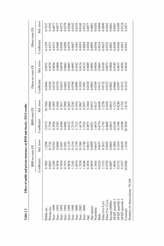
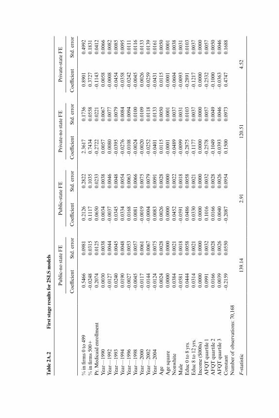
Table 2.3 presents the results from the second stage of the two- stage least squares (2SLS) regressions. Appendix table 2A.2 presents the fi rst stage results. The aim of these regressions is to estimate the causal effect of public and private insurance on BMI and obesity. The fi rst model presents results from the regression model without state fi xed effects. The results show that both private and public insurance have no statistically signifi cant effect on BMI. The point estimates for both public and private insurance are positive, but are estimated imprecisely. This is despite the strong predictive power of the instruments in the fi rst stage [F- stat � 139].
The next model includes state fi xed effects to capture time invariant
Tab
le 2
.3
Eff
ect o
f pu
blic
and
pri
vate
insu
ranc
e on
BM
I an
d ob
esit
y: 2
SL
S re
sult
s
BM
I- no
sta
te F
EB
MI-
stat
e F
EO
bese
- no
stat
e F
EO
bese
- sta
te F
E
Coe
ffici
ent
St
d. e
rror
C
oeffi
cien
t
Std.
err
or
Coe
ffici
ent
St
d. e
rror
C
oeffi
cien
t
Std.
err
or
Pub
lic in
s.0.
7002
1.22
98–3
.817
210
.742
6–0
.084
00.
0931
–0.1
239
0.78
31P
riva
te in
s.0.
9065
0.77
41–7
.778
64.
8906
0.01
680.
0570
–0.4
573
0.35
95Y
ear—
1990
0.22
080.
0765
0.29
260.
1095
0.01
190.
0056
0.01
510.
0077
Yea
r—19
920.
5856
0.08
890.
5303
0.10
860.
0330
0.00
660.
0300
0.00
77Y
ear—
1993
0.70
540.
1047
0.43
640.
3817
0.04
150.
0078
0.01
880.
0272
Yea
r—19
940.
7935
0.10
910.
6006
0.39
000.
0485
0.00
820.
0298
0.02
79Y
ear—
1996
0.98
360.
1129
0.81
220.
2803
0.05
250.
0085
0.03
780.
0200
Yea
r—19
981.
2102
0.12
161.
2379
0.22
450.
0708
0.00
920.
0687
0.01
62Y
ear—
2000
1.60
740.
1339
1.71
210.
1918
0.09
990.
0102
0.10
410.
0139
Yea
r—20
021.
7830
0.15
061.
6174
0.20
670.
1029
0.01
140.
0919
0.01
48Y
ear—
2004
1.86
440.
1740
1.57
630.
2957
0.10
910.
0132
0.08
890.
0212
Age
0.38
580.
0652
0.49
750.
1064
0.02
300.
0049
0.02
840.
0077
Age
squ
are
–0.0
039
0.00
09–0
.005
10.
0013
–0.0
002
0.00
01–0
.000
30.
0001
Non
whi
te1.
3416
0.06
571.
0474
0.41
270.
0789
0.00
500.
0556
0.02
95M
ale
0.82
240.
0857
0.47
740.
6630
–0.0
151
0.00
65–0
.021
40.
0484
Edu
c 0
to 8
yrs
.1.
1532
0.26
15–1
.170
31.
2250
0.07
320.
0188
–0.0
633
0.08
90E
duc
8 to
12
yrs.
0.47
300.
0959
–0.4
040
0.50
380.
0322
0.00
72–0
.022
20.
0363
Inco
me
($00
0s)
–0.0
007
0.00
020.
0013
0.00
12–0
.000
10.
0000
0.00
010.
0001
AF
QT
qua
rtile
11.
0038
0.20
04–0
.814
01.
1223
0.06
660.
0149
–0.0
549
0.08
01A
FQ
T q
uart
ile 2
0.67
520.
1019
–0.1
584
0.42
490.
0397
0.00
75–0
.010
60.
0309
AF
QT
qua
rtile
30.
3557
0.06
580.
0390
0.17
030.
0215
0.00
500.
0023
0.01
24C
onst
ant
14.8
588
1.21
6420
.583
03.
4176
–0.4
152
0.09
10–0
.076
10.
2477
Num
ber
of o
bser
vati
ons:
70,
168
54 Jay Bhattacharya, M. Kate Bundorf, Noemi Pace, and Neeraj Sood
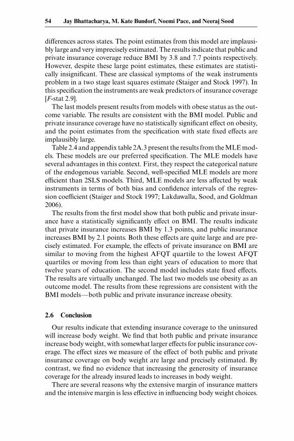
differences across states. The point estimates from this model are implausi-bly large and very imprecisely estimated. The results indicate that public and private insurance coverage reduce BMI by 3.8 and 7.7 points respectively. However, despite these large point estimates, these estimates are statisti-cally insignifi cant. These are classical symptoms of the weak instruments problem in a two stage least squares estimate (Staiger and Stock 1997). In this specifi cation the instruments are weak predictors of insurance coverage [F- stat 2.9].
The last models present results from models with obese status as the out-come variable. The results are consistent with the BMI model. Public and private insurance coverage have no statistically signifi cant effect on obesity, and the point estimates from the specifi cation with state fi xed effects are implausibly large.
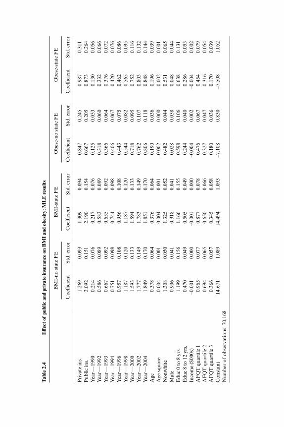
Table 2.4 and appendix table 2A.3 present the results from the MLE mod-els. These models are our preferred specifi cation. The MLE models have several advantages in this context. First, they respect the categorical nature of the endogenous variable. Second, well- specifi ed MLE models are more efficient than 2SLS models. Third, MLE models are less affected by weak instruments in terms of both bias and confi dence intervals of the regres-sion coefficient (Staiger and Stock 1997; Lakdawalla, Sood, and Goldman 2006).
The results from the fi rst model show that both public and private insur-ance have a statistically signifi cantly effect on BMI. The results indicate that private insurance increases BMI by 1.3 points, and public insurance increases BMI by 2.1 points. Both these effects are quite large and are pre-cisely estimated. For example, the effects of private insurance on BMI are similar to moving from the highest AFQT quartile to the lowest AFQT quartiles or moving from less than eight years of education to more that twelve years of education. The second model includes state fi xed effects. The results are virtually unchanged. The last two models use obesity as an outcome model. The results from these regressions are consistent with the BMI models—both public and private insurance increase obesity.
2.6 Conclusion
Our results indicate that extending insurance coverage to the uninsured will increase body weight. We fi nd that both public and private insurance increase body weight, with somewhat larger effects for public insurance cov-erage. The effect sizes we measure of the effect of both public and private insurance coverage on body weight are large and precisely estimated. By contrast, we fi nd no evidence that increasing the generosity of insurance coverage for the already insured leads to increases in body weight.
There are several reasons why the extensive margin of insurance matters and the intensive margin is less effective in infl uencing body weight choices.
Tab
le 2
.4
Eff
ect o
f pu
blic
and
pri
vate
insu
ranc
e on
BM
I an
d ob
esit
y: M
LE
resu
lts
BM
I- no
sta
te F
EB
MI-
stat
e F
EO
bese
- no
stat
e F
EO
bese
- sta
te F
E
Coe
ffici
ent
St
d. e
rror
C
oeffi
cien
t
Std.
err
or
Coe
ffici
ent
St
d. e
rror
C
oeffi
cien
t
Std.
err
or
Pri
vate
ins.
1.26
90.
093
1.30
90.
094
0.84
70.
245
0.98
70.
311
Pub
lic in
s.2.
092
0.15
12.
190
0.15
40.
667
0.20
50.
873
0.26
4Y
ear—
1990
0.21
40.
076
0.21
70.
076
0.12
50.
053
0.13
00.
056
Yea
r—19
920.
586
0.08
90.
583
0.08
90.
318
0.06
00.
332
0.06
6Y
ear—
1993
0.66
70.
092
0.65
50.
092
0.36
60.
064
0.37
60.
072
Yea
r—19
940.
751
0.09
80.
744
0.09
80.
406
0.06
70.
420
0.07
6Y
ear—
1996
0.95
70.
108
0.95
60.
108
0.44
30.
075
0.46
20.
086
Yea
r—19
981.
187
0.12
01.
187
0.12
00.
544
0.08
20.
565
0.09
5Y
ear—
2000
1.59
30.
133
1.59
40.
133
0.71
80.
095
0.75
20.
116
Yea
r—20
021.
777
0.14
91.
783
0.14
90.
762
0.10
70.
803
0.13
2Y
ear—
2004
1.84
90.
170
1.85
10.
170
0.80
60.
118
0.84
80.
144
Age
0.37
80.
064
0.37
60.
064
0.19
00.
036
0.19
60.
039
Age
squ
are
–0.0
040.
001
–0.0
040.
001
–0.0
020.
000
–0.0
020.
001
Non
whi
te1.
308
0.05
01.
325
0.05
20.
482
0.04
40.
531
0.06
5M
ale
0.90
60.
041
0.91
80.
041
0.02
80.
038
0.04
80.
044
Edu
c 0
to 8
yrs
.1.
199
0.15
61.
166
0.15
50.
598
0.10
60.
638
0.13
1E
duc
8 to
12
yrs.
0.47
00.
049
0.50
50.
049
0.24
40.
040
0.28
60.
053
Inco
me
($00
0s)
–0.0
010.
000
–0.0
010.
000
–0.0
040.
002
–0.0
040.
002
AF
QT
qua
rtile
10.
965
0.07
70.
877
0.07
80.
476
0.06
70.
454
0.07
9A
FQ
T q
uart
ile 2
0.69
40.
065
0.65
00.
066
0.32
70.
047
0.31
60.
054
AF
QT
qua
rtile
30.
366
0.05
70.
345
0.05
80.
180
0.03
60.
170
0.03
9C
onst
ant
14.6
711.
089
14.4
941.
093
–7.1
080.
830
–7.5
081.
052
Num
ber
of o
bser
vati
ons:
70,
168
56 Jay Bhattacharya, M. Kate Bundorf, Noemi Pace, and Neeraj Sood
First, changes in the intensive margin of insurance likely have a smaller effect on changes in expected out- of- pocket medical expenditures due to obesity. This means that changes in the intensive margin of insurance produce weaker fi nancial incentives to change body weight. Second, changes in the extensive margin of insurance might be more salient to consumers; conse-quently, such changes might affect behavior more than changes in insurance benefi ts. Finally, risk- averse consumers might respond more to changes in the likelihood of large losses. Changes in the intensive margin of insurance do affect the probability of catastrophic out- of- pocket expenditures, thus they might not infl uence body weight choices by much. One interpretation of our fi ndings is that large changes in fi nancial incentives (such as those encountered along the extensive margin) affect body weight outcomes, while smaller changes in fi nancial incentives (such as those encountered along the intensive margin) do not.
While our results indicate that insurance increases obesity, other authors have come to a different conclusion using a similar approach (Rashad and Markowitz 2010). We demonstrate that the difference is likely due to the method of estimation. When we estimate the model using two- stage least squares, which does not account for the discrete nature of the endogenous indicator of health insurance, our estimates are similar in the sense that we fi nd little evidence that body weight is elastic with respect to insurance cov-erage. Adopting an alternative maximum likelihood method of estimation, which handles explicitly the discrete endogenous variable and is more robust to weak instruments problem, we reach a different conclusion. Body weight is responsive to health insurance coverage in these models. The estimate is both relatively large in magnitude and precise, and does not vary across the different model specifi cations.
Our estimates suggest that, by insulating people from the costs of obesity- related medical care expenditures, insurance coverage expansions create moral hazard in behaviors related to body weight. These effects are larger in public insurance programs where premiums are not risk- adjusted, and smaller in private insurance markets where the obese might pay for incre-mental medical care costs in the form of lower wages (Bhattacharya and Bundorf 2009). By contrast, our estimates also suggest that making insur-ance more generous has no effect on body weight. Taken together, these fi ndings indicate that providing incentives for healthy behaviors such as risk- rating insurance premiums in private may be effective in reducing body weight in the population (though Bhattacharya and Bundorf [2009] fi nd that employer provided health insurance is already implicitly risk- rated for obesity). Policies that impose costs on increases in body weight among those with public coverage may also reduce body weight, though in that case equity concerns are certain to be important in the policy discussion. The policy challenge will be to design mechanisms that impose costs along the extensive
Does Health Insurance Make You Fat? 57
margin, which given our results are likely to be effective, but not along the intensive margin, which are not.
Appendix
A Characterization of the Social Optimum
In this section, we derive necessary conditions characterizing the socially optimal level of weight loss for a society of j � 1 . . . J individuals. Each has the following expected utility, taken from equation (1):
(A.1) EUj � �ii=1
N
∑ (W0j �j)U(Cij) �(�j).
We defi ne total social welfare, , as the sum of expected utilities over all individuals in the society:
(A.2) � � jj=1
J
∑ EUj.
In equation (A.2), �j represents the Pareto weight that individual j has in the social welfare function. In the social budget constraint, total income equals total expenditures on consumption plus total medical expenditures over all individuals. Both income and the distribution of medical expendi-tures depend upon body weight decisions:
(A.3) j=1
J
∑�I(W0j �j) �ii=1
N
∑ (W0j �j)(Mi � Cij)� � 0.
Equation (A.3) builds in our assumption that expectations about the distribution of medical expenditures in the population correspond to the observed distribution of expenditures.
The social problem is to pick consumption and body weight for all indi-viduals in every state of the world—{Cij, �j} �i, j—to maximize subject to the social budget constraint. To this end, we construct the following Lagrangian function, where � is the multiplier associated with the social budget constraint, (A- 3):
(A.4) L � � j�ii=1
N
∑j=1
J
∑ (W0j �j)U(Cij) �j�(�j)
� �j=1
J
∑�I(W0j �j) �ii=1
N
∑ (W0j �j)(Mi � Cij)�.
There are two sets of fi rst order conditions:
58 Jay Bhattacharya, M. Kate Bundorf, Noemi Pace, and Neeraj Sood
(A.5) ∂L�∂Cij
� �jU�(Cij) � � � 0 �i, j, and
(A.6) ∂L�∂�j
� i=1
N
∑��i(W0j �j)�jU(Cij) �j��(�j)
� ��I�(W0j �j) � i=1
N
∑��i(W0j �j)(Mi � Cij)� � 0 �j.
An immediate implication of equation (A.5) is that at the social optimum, each individual j in the society must set his (or her) consumption level to the same value, say Cj
∗, across all the N different health states:
(A.7) Cij �Cj∗ �i, j.
Applying equation (A.7) to equation (A.6) yields the following:
(A.8) (�jU(Cj∗) � �Cj
∗)i=1
N
∑��i(W0j �j) �j��(�j)
� ��I�(W0j �j) � Mii=1
N
∑ ��i(W0j �j)� � 0 �j.
By defi nition, Ni�1�i(W0j – �j) � 1, so we have N
i�1�j�(W0j – �j) � 0. Further-more, differentiating equation (7), which defi nes the risk- adjusted premium, P(W0j – �j), yields the fact that:
(A.9) P�(W0j �j) � i=1
N
∑��i(W0j �j)Mi �j.
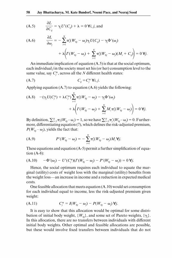
These equations and equation (A- 5) permit a further simplifi cation of equa-tion (A- 8):
(A.10) ��(�j) U�(Cj∗)(I�(W0j �j) P�(W0j �j)) � 0 �j.
Hence, the social optimum requires each individual to equate the mar-ginal (utility) costs of weight loss with the marginal (utility) benefi ts from the weight loss—an increase in income and a reduction in expected medical costs.
One feasible allocation that meets equation (A.10) would set consumption for each individual equal to income, less the risk- adjusted premium given weight:
(A.11) Cj∗ � I(W0j �j) P(W0j �j) �j.
It is easy to show that this allocation would be optimal for some distri-bution of initial body weight, {W0j}, and some set of Pareto weights, {�j}. In this allocation, there are no transfers between individuals with different initial body weights. Other optimal and feasible allocations are possible, but these would involve fi xed transfers between individuals that do not
Tab
le 2
A.1
R
AN
D e
nrol
lees
dem
ogra
phic
and
hea
lth
stat
us c
ovar
iate
s ar
e ba
lanc
ed a
t sta
rt o
f ex
peri
men
t
All
F
ree
25
%
50%
95
%
Indi
vidu
al
N2,
461
824
492
167
442
536
Age
(yea
rs)
37.3
637
.85
36.9
138
.35
37.3
536
.70
(11.
18)
(11.
51)
(10.
69)
(11.
16)
(11.
14)
(11.
14)
Edu
cati
on (y
ears
of
scho
ol c
ompl
eted
)12
.34
12.1
512
.48
12.4
712
.41
12.3
9(3
.03)
(3.2
0)(2
.91)
(3.0
7)(2
.87)
(3.0
0)F
amily
inco
me
(yea
r pr
eced
ing
enro
llmen
t)11
,524
11,1
3511
,879
∗12
,993
∗∗11
,654
11,2
29(5
,772
)(5
,734
)(5
,785
)(5
,825
)(5
,791
)(5
,710
)P
arti
cipa
tion
ince
ntiv
e off
ered
at e
nrol
lmen
t46
1.17
175.
3270
2.81
∗∗81
1.14
∗∗73
3.22
∗∗34
5.40
(370
)(2
38)
(281
)(3
24)
(348
)(2
11)
Rac
e—w
hite
0.88
0.87
0.87
0.92
0.86
0.88
Rac
e—bl
ack
0.11
0.12
0.11
0.07
0.13
0.11
Rac
e—ot
her
0.01
0.01
0.02
0.01
0.01
0.01
Mar
ried
0.80
0.81
0.81
0.83
0.77
0.79
Fem
ale
0.54
0.54
0.53
0.56
0.57
0.53
Self
rep
orte
d he
alth
sta
tus—
exce
llent
0.45
0.45
0.45
0.49
0.46
0.45
Self
rep
orte
d he
alth
sta
tus—
good
0.43
0.42
0.43
0.40
0.43
0.45
Self
rep
orte
d he
alth
sta
tus—
fair
0.09
0.10
0.10
0.10
0.09
0.07
Self
rep
orte
d he
alth
sta
tus—
poor
0.02
0.03
0.01
0.02
0.02
0.02
Self
rep
orte
d he
alth
sta
tus—
mis
sing
0.
01
0.01
0.
01
—
0.01
0.
00
Not
e: D
ashe
d ce
ll m
eans
that
ther
e ar
e no
obs
erva
tion
s in
that
cat
egor
y (5
0 pe
rcen
t cop
aym
ent)
who
had
a m
issi
ng v
alue
for
self
- rep
orte
d he
alth
sta
tus.
∗∗Si
gnifi
cant
at t
he 5
per
cent
leve
l.∗ S
igni
fi can
t at t
he 1
0 pe
rcen
t lev
el.
Tab
le 2
A.2
F
irst
sta
ge re
sult
s fo
r 2S
LS
mod
els
Pub
lic- n
o st
ate
FE
Pub
lic- s
tate
FE
Pri
vate
- no
stat
e F
EP
riva
te- s
tate
FE
Coe
ffici
ent
Std.
err
or
Coe
ffici
ent
Std.
err
or
Coe
ffici
ent
Std.
err
or
Coe
ffici
ent
Std.
err
or
% in
fi rm
s 0
to 4
990.
5466
0.09
810.
2126
0.28
222.
3617
0.17
360.
8901
0.49
92%
in fi
rms
500�
–0.0
248
0.03
150.
1117
0.10
350.
7434
0.05
580.
3727
0.18
31P
r. M
edic
aid
enro
llmen
t0.
2074
0.01
250.
0650
0.02
33–0
.272
20.
0221
–0.1
143
0.04
12Y
ear—
1990
0.00
300.
0038
0.00
340.
0038
0.00
570.
0067
0.00
580.
0066
Yea
r—19
92–0
.012
70.
0044
–0.0
037
0.00
460.
0080
0.00
77–0
.000
80.
0082
Yea
r—19
930.
0240
0.00
450.
0345
0.00
48–0
.039
50.
0079
–0.0
454
0.00
85Y
ear—
1994
0.01
900.
0048
0.03
340.
0054
–0.0
276
0.00
84–0
.035
80.
0095
Yea
r—19
96–0
.002
70.
0053
0.01
680.
0063
–0.0
108
0.00
94–0
.024
20.
0111
Yea
r—19
98–0
.004
50.
0057
0.00
810.
0066
–0.0
024
0.01
00–0
.004
50.
0116
Yea
r—20
00–0
.011
70.
0061
–0.0
019
0.00
75–0
.002
00.
0109
0.00
260.
0133
Yea
r—20
02–0
.014
40.
0067
–0.0
004
0.00
79–0
.025
20.
0118
–0.0
259
0.01
39Y
ear—
2004
–0.0
124
0.00
750.
0083
0.00
91–0
.040
10.
0133
–0.0
431
0.01
61A
ge0.
0024
0.00
280.
0026
0.00
280.
0115
0.00
500.
0115
0.00
50A
ge s
quar
e0.
0000
0.00
000.
0000
0.00
00–0
.000
10.
0001
–0.0
001
0.00
01N
onw
hite
0.03
840.
0021
0.04
520.
0022
–0.0
489
0.00
37–0
.060
40.
0038
Mal
e–0
.058
10.
0018
–0.0
591
0.00
18–0
.009
90.
0031
–0.0
093
0.00
31E
duc
0 to
8 y
rs.
0.04
440.
0058
0.04
860.
0058
–0.2
875
0.01
03–0
.289
10.
0103
Edu
c 8
to 1
2 yr
s.0.
0314
0.00
210.
0330
0.00
21–0
.117
70.
0037
–0.1
217
0.00
37In
com
e ($
000s
)0.
0000
0.00
000.
0000
0.00
000.
0000
0.00
000.
0000
0.00
00A
FQ
T q
uart
ile 1
0.09
910.
0032
0.10
160.
0032
–0.2
578
0.00
57–0
.253
20.
0057
AF
QT
qua
rtile
20.
0166
0.00
280.
0166
0.00
28–0
.104
90.
0049
–0.1
000
0.00
50A
FQ
T q
uart
ile 3
0.00
390.
0026
0.00
400.
0026
–0.0
393
0.00
46–0
.036
30.
0046
Con
stan
t–0
.215
90.
0550
–0.2
087
0.09
540.
1500
0.09
730.
4747
0.16
88N
umbe
r of
obs
erva
tion
s: 7
0,16
8
F- s
tati
stic
13
9.14
2.
91
120.
51
4.52
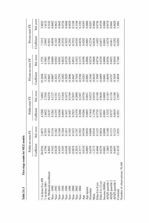
Tab
le 2
A.3
F
irst
sta
ge re
sult
s fo
r M
LE
mod
els
Pub
lic- n
o st
ate
FE
Pub
lic- s
tate
FE
Pri
vate
- no
stat
e F
EP
riva
te- s
tate
FE
Coe
ffici
ent
St
d. e
rror
C
oeffi
cien
t
Std.
err
or
Coe
ffici
ent
St
d. e
rror
C
oeffi
cien
t
Std.
err
or
% in
fi rm
s 0
to 4
9930
.855
62.
4072
4.32
087.
6902
19.1
894
1.37
517.
3312
3.90
23%
in fi
rms
500�
4.37
960.
7933
1.60
222.
7916
5.29
150.
3981
2.99
911.
4132
Pr.
Med
icai
d en
rollm
ent
4.48
420.
3433
2.61
470.
6278
–0.9
681
0.17
00–0
.503
10.
3142
Yea
r—19
900.
3162
0.11
160.
3262
0.11
270.
0007
0.04
890.
0050
0.04
92Y
ear—
1992
–0.0
120
0.12
620.
1355
0.13
51–0
.102
10.
0582
–0.1
165
0.06
21Y
ear—
1993
0.41
930.
1160
0.62
460.
1271
–0.2
763
0.05
81–0
.264
80.
0642
Yea
r—19
940.
3185
0.12
440.
6093
0.14
16–0
.248
20.
0632
–0.2
332
0.07
26Y
ear—
1996
–0.0
108
0.14
130.
3621
0.16
72–0
.302
90.
0729
–0.3
035
0.08
68Y
ear—
1998
0.03
820.
1503
0.36
870.
1769
–0.3
046
0.07
95–0
.250
10.
0929
Yea
r—20
00–0
.081
80.
1633
0.29
230.
2035
–0.4
447
0.09
11–0
.355
20.
1108
Yea
r—20
02–0
.283
50.
1747
0.13
700.
2090
–0.7
410
0.10
12–0
.674
30.
1184
Yea
r—20
04–0
.377
70.
1922
0.20
900.
2387
–0.9
700
0.11
75–0
.887
60.
1392
Age
0.01
100.
0744
0.02
060.
0756
0.02
830.
0390
0.02
920.
0393
Age
squ
are
0.00
050.
0010
0.00
030.
0011
–0.0
001
0.00
06–0
.000
10.
0006
Non
whi
te0.
6359
0.04
980.
7414
0.05
23–0
.156
60.
0274
–0.2
274
0.02
87M
ale
–1.2
173
0.05
10–1
.279
80.
0518
–0.8
610
0.06
00–0
.863
80.
0606
Edu
c 0
to 8
yrs
–0.4
444
0.11
25–0
.371
80.
1149
–1.3
949
0.07
34–1
.418
20.
0736
Edu
c 8
to 1
2 yr
s0.
0239
0.06
140.
0572
0.06
30–0
.600
90.
0330
–0.6
471
0.03
30In
com
e ($
000s
)–0
.000
10.
0000
–0.0
001
0.00
000.
0001
0.00
000.
0001
0.00
00A
FQ
T q
uart
ile 1
1.24
650.
1160
1.33
520.
1183
–1.0
656
0.05
56–1
.027
40.
0574
AF
QT
qua
rtile
20.
8320
0.11
150.
8737
0.11
36–0
.674
70.
0432
–0.6
411
0.04
41A
FQ
T q
uart
ile 3
0.66
930.
1125
0.68
190.
1140
–0.3
459
0.04
16–0
.329
20.
0420
Con
stan
t–1
1.41
181.
4551
–6.5
811
2.59
57–3
.405
40.
7344
–0.8
305
1.30
61N
umbe
r of
obs
erva
tion
s: 7
0,16
8
62 Jay Bhattacharya, M. Kate Bundorf, Noemi Pace, and Neeraj Sood
depend upon fi nal body weight (though they might depend upon initial body weight). Optimal transfers would clearly vary with {�j}, though all optimal allocations would need to obey condition (A.10).
References
Anderson, P. M., K. F. Butcher, and P. B. Levine. 2003. Maternal employment and overweight children. Journal of Health Economics 22 (3): 477– 504.
Bertakis, K. D., and R. Azari. 2005. Obesity and the use of health care services. Obesity Research 13 (2): 372– 9.
Bhat, C. R. 2001. Quasi- random maximum simulated likelihood estimation of the mixed multinomial logit model. Transportation Research: Part B 35:677- 93.
Bhattacharya, J., and K. Bundorf. 2009. The incidence of the healthcare costs of obesity. Journal of Health Economics 28 (3): 649– 58.
Bhattacharya, J., and D. Lakdawalla. 2006. Does medicare benefi t the poor? Journal of Public Economics 90 (1- 2): 277– 92.
Bhattacharya, J., and N. Sood. 2007. Health insurance and the obesity externality. Advances in Health Services Research 17:279– 318.
Brownell, K., and K. B. Horgen. 2004. Food fi ght: The inside story of the food indus-try, America’s obesity crisis, and what we can do about it. New York: McGraw- Hill.
Bungam, T., M. Satterwhite, A. W. Jackson, and J. R. Morrow. 2003. The relation-ship of body mass index, medical costs, and job absenteeism. American Journal of Health Behavior 27 (4): 456– 62.
Burton, W. N., C. Y. Chen, A. B. Schultz, and D. W. Edington. 1998. The economic costs associated with body mass index in a workplace. Journal of Occupational and Environmental Medicine 40 (9): 786– 92.
Cawley, J. 2000. An instrumental variables approach to measuring the effect of body weight on employment disability. Health Services Research 35 (5 Pt 2): 1159– 79.
———. 2004. An economic framework for understanding physical activity and eat-ing behaviors. American Journal of Preventive Medicine 27 (3S): 117– 25.
Cutler, D., E. Glaeser, and J. Shapiro. 2003. Why have Americans become more obese? Journal of Economic Perspectives 17 (3): 93– 118.
Dave, D., and R. Kaestner. 2009. Health insurance and ex ante moral hazard: Evi-dence from Medicare. International Journal of Health Care Finance and Econom-ics 9 (4): 367– 90.
Daviglus, M. L., K. Liu, L. L. Yan, A. Pirzada, L. Manheim, W. Manning, and D. B. Garside. 2004. Relation of body mass index in young adulthood and middle age to Medicare expenditures in older Age. Journal of the American Medical Associa-tion 292 (22): 2243– 749.
Deb, P., and P. K. Trivedi. 1997. Demand for medical care by the elderly: A fi nite mixture approach. Journal of Applied Econometrics 12 (3): 313– 36.
———. 2006. Specifi cation and simulated likelihood estimation of a non- normal treatment- outcome model with selection: Application to health care utilization. Econometrics Journal 9:307– 31.
Elmer, P. J., J. B. Brown, G. A. Nichols, and G. Oster. 2004. Effects of weight gain on medical care costs. International Journal of Obesity 28:1365– 73.
Finkelstein, E. A., I. C. Fiebelkorn, and G. Wang. 2003. National medical spending
Does Health Insurance Make You Fat? 63
attributable to overweight and obesity: How much, and who’s paying? Health Affairs W3- 219- 26.
———. 2004. State- level estimates of annual medical expenditures attributable to obesity. Obesity Research 12 (1): 18– 24.
Finkelstein, E. A., C. J. Ruhm, and K. M. Kosa. 2005. Economic causes and conse-quences of obesity. Annual Review of Public Health 26:239– 57.
Gouriéroux, C., and A. Monfort. 1996. Simulation based econometrics methods. New York: Oxford University Press.
Gruber, J. 2000. Health insurance and the labor market. 2000. In Handbook of health economics, ed. A. J. Cuyler and J. P. Newhouse, 645– 700. Amsterdam: Elsevier.
Katzmarzyk, P. T., and I. Janssen. 2004. The economic costs associated with physical inactivity and obesity in Canada: An update. Canadian Journal of Applied Physi-ology 29 (1): 90– 115.
Keeler, E. B., W. G. Manning, J. P. Newhouse, E. M. Sloss, and J. Wasserman. 1989. The external costs of a sedentary lifestyle. American Journal of Public Health 79:975– 81.
Keenan, P. S., M. J. Buntin, T. G. McGuire, and J. P. Newhouse. 2001. The preva-lence of formal risk adjustment in health plan purchasing. Inquiry 38 (Fall): 245– 59.
Lakdawalla, D., and T. Philipson. 2002. The growth of obesity and technological change: A theoretical and empirical examination. NBER Working Paper no. 8946. Cambridge, MA: National Bureau of Economic Research, May.
Lakdawalla, D., N. Sood, and D. Goldman. 2006. HIV breakthroughs and risky sexual behavior. Quarterly Journal of Economics 121 (3): 1063– 102.
Manning, W. G., E. B. Keeler, J. P. Newhouse, E. M. Sloss, and J. Wasserman. 1991. The costs of poor health habits. Cambridge, MA: Harvard University Press.
McClellan, M., and J. Skinner. 1999. Medicare reform: Who pays and who benefi ts? Health Affairs 18 (1): 48– 62.
———. 2006. The incidence of Medicare. Journal of Public Economics 90 (January): 257– 76.
McFadden, D. 1980. Econometric models for probabilistic choice among products. Journal of Business 53:S13– S29.
Mokdad, A. H., M. K. Serdula, W. H. Dietz, B. A. Bowman, J. S. Marks, and J. P. Koplan. 1999. The spread of the obesity epidemic in the United States, 1991– 1998. Journal of the American Medical Association 282 (16): 1519– 22.
Mokdad, A. H., E. S. Ford, B. A. Bowman, W. H. Dietz, F. Vinicor, V. S. Bales, and J. S. Markes. 2003. Prevalence of obesity, diabetes, and obesity- related health risk factors, 2001. Journal of the American Medical Association 289 (1): 76– 9.
Musich, S., C. Lu, T. McDonald, L. J. Champagne, and D. W. Edington. 2004. Asso-ciation of additional health risks on medical charges and prevalence of diabetes within body mass index categories. American Journal of Health Promotion 18 (3): 264– 68.
Nestle, M. 2003. Food politics: How the food industry infl uences nutrition and health. Berkeley, CA: University of California Press.
Newhouse, J. P., and Insurance Experiment Group. 1993. Free for all? Lessons from the RAND health insurance experiment. Cambridge, MA: Harvard University Press.
Pagan, J. A., and A. Davila. 1997. Obesity, occupational attainment, and earnings. Social Science Quarterly 78 (3): 756– 70.
Quesenberry, C. P., Jr., B. Caan, and A. Jacobson. 1998. Obesity, health services use, and health care costs among members of a health maintenance organization. Archives of Internal Medicine 158 (5): 466– 72.
64 Jay Bhattacharya, M. Kate Bundorf, Noemi Pace, and Neeraj Sood
Raebel, M. A., D.C. Malone, D. A. Conner, S. Xu, J. A. Porter, and F. A. Lanty. 2004. Health services use and health care costs of obese and non- obese individu-als. Archives of Internal Medicine 164:2135– 40.
Rashad, I. K., and S. Markowitz. 2010. Incentives in obesity and insurance. Inquiry 46 (4): 418– 32.
Register, C. A., and D. R. Williams. 1990. Wage effects of obesity among young workers. Social Science Quarterly 71 (1): 130– 41.
Rosen, S. 1986. The theory of equalizing differences. In Handbook of labor econom-ics, ed. O. Ashenfelter and D. Card, 641– 92. Amsterdam: Elsevier.
Sander, B., and R. Bergemann. 2003. Economic burden of obesity and its complica-tions in Germany. European Journal of Health Economics 4 (4): 248– 53.
Staiger, D., and J. H. Stock. 1997. Instrumental variables regression with weak instruments. Econometrica 65 (3): 557– 86.
Sturm, R. 2002. The effects of obesity, smoking, and drinking on medical problems and costs. Health Affairs 21 (2): 245– 53.
Thompson, D., J. B. Brown, G. A. Nichols, P. J. Elmer, and G. Oster. 2001. Body mass index and future healthcare costs: A retrospective cohort study. Obesity Research 9 (3): 210– 18.
Thorpe, K. E., C. S. Florence, D. H. Howard, and P. Joski. 2004. The impact of obesity on rising medical spending. Health Affairs Web Exclusive (W4): 480– 6.
Train, K. 2002. Discrete choice methods with simulation. New York: Cambridge Uni-versity Press.
Wang, F., A. B. Schultz, S. Musich, T. McDonald, D. Hirschland, and D. W. Eding-ton. 2003. The relationship between National Heart, Lung, and Blood Institute weight guidelines and concurrent medical costs in a manufacturing population. American Journal of Health Promotion 17 (3): 183– 9.
Wolf, A. M., and G. A. Colditz. 1994. The cost of obesity. Pharmacoeconomics 5 (Suppl 1): 34– 7.
Related Documents