DOES A PORTFOLIO OF GROWTH STOCKS OUTPERFORM ...

DOES A PORTFOLIO OF

GROWTH STOCKS

OUTPERFORM A PORTFOLIO OF VALUE

STOCKS?

Evidence from Sweden and

Norway

Lina Andersson, Daniella Holmgren

Department of Business Administration

Civilekonomprogrammet

Degree Project, 30 Credits, Spring 2022

Supervisor: Siarhei Manzhynski

[This page was intentionally left blank]

Acknowledgement We would like to thank our supervisor Siarhei Manzhynski and all the participants at

the seminars for providing us with important feedback to improve our thesis. Also, we

would like to thank each other for the partnership and our different knowledge during

the work with the thesis, which made it possible to complete it.

Umeå, May 2022

Lina Andersson Daniella Holmgren

Abstract A high return is a driving factor for most investors. The ways to reach success are many

and different investment strategies on how to earn high returns have been discussed for

decades. Value stocks (low P/E ratios) and growth stocks (high P/E ratios) are two

strategies among the investment area with different and contrary results on which

strategy can give the highest possible return. However, studies of the P/E effect have

shown different results the last years compared to previous findings of a value premium

for low P/E stocks, with trends of a higher return for growth stocks compared to value

stocks. This led us to the research question “Does a portfolio of growth stocks present a

higher return than a portfolio with value stocks on the Swedish and Norwegian stock

markets?”.

The problem that the study aims to answer is therefore if a portfolio of growth stocks

provides a higher return than a portfolio of value stocks between the years 2001-2021.

The long timespan will give us the opportunity to evaluate the stock markets during

both booms and busts. Our study is made on historical data on the Swedish and the

Norwegian stock markets since we found a lack of previous research in these countries

within the research area. To fulfil the purpose of the study and to answer the research

question, a quantitative method is used with historical data provided from Eikon

(Thomson Reuters DataStream) where firms are sorted on the P/E ratios and after that

growth and value portfolios are created. We will present both the actual return as well

as a risk adjusted return for the stocks. The risk adjusted returns are conducted by using

the financial measurements Sharpe ratio and Jensen’s alpha.

The result of the study shows that on a 5 % significance level, growth stocks presented a

higher actual return than value stocks for both Sweden and Norway. The same evidence

was found for the returns for growth stocks compared to market index. Though, when

testing the risk adjusted returns, the null hypothesis could not be rejected, which implies

that a statistical difference between the portfolios could not be found.

Keywords: Growth stocks, value stocks, P/E ratio, Sharpe ratio, Jensen’s alpha,

behavioural finance, efficient market hypothesis, financial crises.

Table of Contents

1.Introduction .....................................................................................................................1

1.1 Problem background: .......................................................................................................... 1

1.2 Purpose: .............................................................................................................................. 3

1.3 Research gap and contribution ........................................................................................... 3

1.4 Delimitations ....................................................................................................................... 4

2. Theoretical method .........................................................................................................5

2.1 Research philosophies ......................................................................................................... 5

2.1.1 Epistemology ................................................................................................................ 6

2.1.2 Ontology ....................................................................................................................... 6

2.2 Research Approach ............................................................................................................. 7

2.3 Research Method ................................................................................................................ 7

2.4 Quality criteria ..................................................................................................................... 8

2.5 Time horizon ........................................................................................................................ 9

2.6 Social & Ethical Research .................................................................................................. 10

2.7 Literature and Data Sources .............................................................................................. 10

2.8 Source criticism ................................................................................................................. 11

2.9 Summary of the theoretical methodology ........................................................................ 12

3. Theoretical point of departure ....................................................................................... 13

3.1 Choice of topic ................................................................................................................... 13

3.2 Growth versus value stocks ............................................................................................... 13

3.3 Fama & French Factor Models .......................................................................................... 15

3.4 Efficient-market hypothesis .............................................................................................. 16

3.5 Random walk theory ......................................................................................................... 18

3.6 Behavioural finance ........................................................................................................... 19

3.7 Modern portfolio theory ................................................................................................... 20

3.8 Sharpe ratio ....................................................................................................................... 21

3.9 Jensen’s alpha ................................................................................................................... 21

3.10 The Magic Formula .......................................................................................................... 22

3.11 Additional research ......................................................................................................... 23

3.12 Summary of theoretical framework ................................................................................ 24

4. Practical method ............................................................................................................ 26

4.1 Data collection................................................................................................................... 26

4.1.1 Sample selection and Creation of portfolios .............................................................. 26

4.1.2 Sample size and the complete portfolios ................................................................... 28

4.2 Returns .............................................................................................................................. 29

4.2.1 Actual returns ............................................................................................................. 29

4.2.2 Risk adjusted return ................................................................................................... 29

4.2.3 Risk-free rate .............................................................................................................. 30

4.2.4 Jensen’s alpha ............................................................................................................ 30

4.2.5 Market index returns ................................................................................................. 31

4.3 Hypothesis ......................................................................................................................... 31

4.4 Normality ........................................................................................................................... 33

4.5 Selection of significance test ............................................................................................. 33

4.5.1 Non-parametric tests ................................................................................................. 33

4.5.2 Parametric tests ......................................................................................................... 34

5. Empirical Findings .......................................................................................................... 35

5.1 Portfolio statistics .............................................................................................................. 35

5.2 Normality testing ............................................................................................................... 37

5.3 Actual returns .................................................................................................................... 38

5.4 Jensen’s Alpha ................................................................................................................... 40

5.5 Risk-adjusted returns ........................................................................................................ 41

5.6 Statistical Significance testing ........................................................................................... 43

5.7 Summary of the hypothesis testing .................................................................................. 46

6. Analysis ......................................................................................................................... 47

6.1 Analysis of the results / hypothesis tests .......................................................................... 47

6.1.1 Hypothesis 1 ............................................................................................................... 47

6.1.2 Hypothesis 2 ............................................................................................................... 48

6.1.3 Hypothesis 3 ............................................................................................................... 49

6.1.4 Hypothesis 4 ............................................................................................................... 49

6.1.5 Hypothesis 5 ............................................................................................................... 50

6.2 The results compared to previous research ...................................................................... 50

6.3 The results compared to relevant theories ....................................................................... 51

7. Conclusion ..................................................................................................................... 53

7.1 General Conclusion ........................................................................................................... 53

7.2 Limitations ......................................................................................................................... 54

7.3 Contribution ...................................................................................................................... 54

7.3.1 Theoretical contribution ............................................................................................ 54

7.3.2 Practical contribution ................................................................................................. 55

7.4 Social and ethical aspects .................................................................................................. 55

7.5 Quality Criteria .................................................................................................................. 56

7.5.1 Reliability .................................................................................................................... 56

7.5.2 Validity ........................................................................................................................ 57

7.6 Suggestion for future research .......................................................................................... 58

Reference list .................................................................................................................... 60

Appendix 1: Risk free rate Sweden and Norway……………………………………………………………………66 Appendix 2: T-test Norway period 1………………………………………………………………….....................66 Appendix 3: T-test Norway period 2……………………………………………………………………………………. 67 Appendix 4: T-test Norway period 3…………………………………………………………………………………….67 Appendix 5: T-test Norway period 4…………………………………………………………………………………….67 Appendix 6: T-test Norway total period……………………………………………………………………………….68 Appendix 7: T-test Sweden period 1……………………………………………………………………………………68 Appendix 8: T-test Sweden period 2……………………………………………………………………………………68 Appendix 9: T-test Sweden period 3…………………………………………………………………………………….69 Appendix 10: T-test Sweden period 4…………………………………………………………………………………..69 Appendix 11: T-test Sweden total period………………………………………………………………………………69

List of figures Figure 1: The ‘research onion’……..……………………………………………………………...…………………….....5 Figure 2: The process of a deductive approach………………………………………..………………….……..…7 Figure 3: Diversification of portfolios based on P/E ratio……………………………………..…………….. 26 Figure 4: Normality testing of portfolios in Sweden…………………………………………….……………….37 Figure 5: Normality testing of portfolios in Sweden………………………………………..…….……………..37 Figure 6: Normality testing of portfolios in Norway…………………………………….…………..…………..38 Figure 7: Normality testing of portfolios in Norway……………………………………..……….……………..38 Figure 8: Average annual return Sweden………………………………………………………………..…………….40 Figure 9: Average annual return Norway……………………………………………………….……….…………….40 Figure 10: Risk free rates for Sweden and Norway……………………………………….……..……………….41 Figure 11: Sharpe ratios Sweden (S) and Norway (N)…………………………………………...………………42 Figure 12: Risk adjusted returns (Sharpe ratio) for Sweden………………………………….………………45 Figure 13: Risk adjusted returns (Sharpe ratio) for Norway…………………………………..……………..46

List of tables Table 1: Summary of the theoretical methodology…………………………………………….……………..…12 Table 2: P/E ratios for Swedish portfolios 2001-2021……………………………………………………………35 Table 3: P/E ratios for Norwegian portfolios 2001-2021…………………………….…………………………36 Table 4: P/E ratios for sub-periods in Sweden………………………………………………………………………37 Table 5: P/E ratios for sub-periods in Norway……………………………………………………………..……….37 Table 6: Actual returns in Sweden…………..................................................................................39 Table 7: Actual returns in Norway………………………………………………………………………………………..39 Table 8: Jensen’s Alpha………………………………………………………………………………………….……………..41 Table 9: Sharpe ratios……………………………………………………………………..…………………………………….42 Table 10: Hypothesis test Norway…………………………………………………………………….…………………..43 Table 11: Hypothesis test Sweden…………………………………………………………………..………………..….44 Table 12: Hypothesis test high P/E towards index……………………………………….……………………….44 Table 13: Hypothesis test low P/E towards index………………………………………..……………………….45 Table 14: Hypothesis test of risk adjusted returns (Sharpe ratio)……………..……………………..….45 Table 15: Summary of the hypotheses tests………………………………………………………………….…..…46

1

1.Introduction This chapter will contain a presentation of the research topic by introducing the

problem background and purpose in relation to the research question. At the end, the

research gap and delimitations for the thesis will be discussed to give the reader a

better overview of what to expect from the study.

1.1 Problem background:

Profit and the return on investment is a driving factor for the most investors who seek to

maximize these in their portfolios by the choice of investments they decide to include.

Though, the range of investors is huge; some do it in their spare time as a hobby while

others ‘put their whole life’ into the market. Even if all individuals have different

preferences when creating their portfolios, these preferences often include the amount

of risk an investor is willing to take and what kind of securities to invest in.

Value and growth stocks are one way to classify stocks and can be used to base the

investment strategies on. There are many ratios that are used for determining these

different stocks, but a common one is the P/E ratio and the P/E effect. In fact, the

discussion of the P/E effect is found as far back as from findings of Basu (1977) and has

after that been widely discussed. The P/E effect is connected to stocks with low P/E

ratios which are usually associated with value stocks. These stocks usually pay

dividends, are trading under their true value, and the return is expected to come when

the stock catches up to the fundamental value (Hayes, 2022). Contrary to value stocks,

there is growth stocks which can be described as stocks in a company that the market

expects to outperform the average growth for the market (Hayes, 2022). Further, growth

stocks are trading at high P/E ratios which often make them look expensive, but if the

expectations are correct, it will be followed by an increasing share price. On the other

hand, if the expected and the realized growth do not continue, the stock price can

instead decline and therefore growth stocks can be considered as a risky investment

(Hayes, 2022).

Selecting between value and growth stocks is interesting, though hard, with the return as

the driving factor among investors, since previous research shows both contrary and

different results. Fama & French (1998) found that value stocks before 1998 performed

better with higher returns than growth stocks. An explanation to that were according to

the authors a correction after an undervaluation of the value stocks, while the growth

stocks were overvalued. Gregory et al. (2003) also found that value stocks outperformed

growth stocks, here on the US market during 1980 to 1998. The same results were

presented for the Australian market which showed that value stocks had a higher return

than growth stocks (Gharghoria et al., 2013).

Though, more recent studies have showed contrary results. Lev & Srivastava (2019)

found evidence that shows an outperformance of growth stocks compared to value

stocks on the US market. The authors even argue that value investing has not been as

successful as earlier among the 10-12 past years. Brindelid & Nilsson (2021) did similar

2

studies, but for the Nordic countries instead and found evidence for value investing

again. They tested The Magic formula, which is a strategy that aims for buying cheap

stocks in terms of a high earnings yield (equivalent to a low P/E-ratio) and a high ROC.

The study showed that portfolios that were created with the Magic Formula beat the

indexes in both Sweden and Norway during the time period 2012-2021, even if Norway

showed a greater return than the rest of the Nordic countries compared to index.

One cause of the more recent findings of lower success for value stocks could be a

result of the low rates the world has faced the last years. As Bratt (2021) explains it, the

expected future returns are higher when the rates are low since future cash flows are

predicted to be high. This can result in higher stock prices for growth stocks since these

often are highly valued with expectations of high future earnings and cash flows (Bratt,

2021). Contrary, when the rates are high, the expected returns and cash flows get lower

since a future discounted cash flow is not worth that much with high rates (Bratt, 2021),

which can result in lower stock prices for growth stocks.

Since the last years have been characterized by low and even negative rates and recent

studies have showed more favourable results for growth stocks, the angle of this thesis

will be to evaluate if growth stocks provide higher returns than value stocks. Research

among the P/E effect and growth versus value stocks have been implied on the US

market and over all on the European market. However, Oslo Børs ASA and Nasdaq

Stockholm have not been the focus in previous research, neither a comparison between

the countries has been found. The fact that previous studies show both contrary and

different results make further research interesting and shows the difficulty of predict the

return of portfolios consisting of growth and value stocks, based on the P/E ratio. Also,

as the countries are similar in size and are close geographically, but the economic and

the leading sectors of the stock markets in the countries differ from each other is an

interesting background for the comparison. Norway is one of the largest economies in

the world with a high export sector consisting of oil and gas, followed by the fishing-

sector (Globalis1, 2021). This of course affects the stock market and for example, the

Norwegian stock market is unique because of the index Oslobørs Seafood Index

(OBSFX) which is an index consisting of stocks of only seafood and particular salmon

(Henriksen, 2016). Sweden on the other hand is one of the most industrialised countries

in Scandinavia with engineering, mine and steel as the main sectors (Globalis2, 2021),

and the stock market of Sweden can also be said to be unique in terms of the high

numbers of small-cap lists and firms, especially growth and innovation firms

(Jinderman, n.d). According to Holliday (2018) is the ratio of market investors and

average interest in the stock market also higher in Sweden compared to Norway, which

can be explained by the larger proportion of microcap operations in Sweden versus

Norway. Also, the small size of various small-scale operations can make it difficult for

fund managers and investors to take significant positions.

Based on the background, the following research question is constructed:

“Does a portfolio of growth stocks present a higher return than a portfolio with value

stocks on the Swedish and Norwegian stock markets?”

3

1.2 Purpose:

The purpose of this study is to evaluate the investing strategies among value and growth

stocks. As stated, the study will examine if a portfolio of growth stocks (high P/E ratio)

produces a higher return than a portfolio of value stocks (low P/E ratios) which will be

done by using historical data from the Norwegian and Swedish stock exchange markets.

The portfolios will also be compared to market indexes to evaluate how these have

presented against index as well, to be able to compare the strategies to previous research

and theories.

The data for this study will be conducted from Oslo Børs ASA and Nasdaq Stockholm

during the period 2001-2021. Since this period both will cover both the Dot-com crisis,

financial crisis 2008-2009 and the Covid-19 pandemic one part of the purpose is also to

evaluate how growth and value portfolios perform during times of financial distress

which will be possible due to the long period of data. Thus, the financial crises will also

be compared to more stable financial periods to evaluate if differences among the

strategies can be found.

1.3 Research gap and contribution

As mentioned in the background, previous research has been conducted on this topic

and the performance of value and growth stocks are well discussed. Though, the results

from previous studies show different and contrary results, which is one argument for

further research among this area. Fama & French (1998); Gregory et al., (2003) among

others found that value stocks outperformed growth stocks in terms of return. Van Dinh

(2021) did not find the same results and stated that a higher return of value portfolios

could not be seen compared to portfolios of growth stocks. Previous research on the

Swedish and Norwegian stock markets among value and growth stocks exists but is not

as expanded as for the rest of the European countries and the US market, neither for our

chosen time period. This research gap became the first inspiration of investigating

Sweden and Norway, as well as the lack of comparisons between the two countries.

Concerning financial crises, which earlier only have been touched upon, will also be

contributively to investigate further. Both Sweden and Norway have their own currency

which is interesting to consider since they might not be as effected as, for example

Finland, when shifts or events happen that affect the euro. According to Holliday (2018)

both Norway and Sweden were able to avoid the worst Eurozone crisis of 2008, since

both countries have their own currency and low debt, compared to much of the Western

countries. Another similarity of the countries is the higher return compared to the

benchmark for real return. The European benchmark for real return, including the Credit

Suisse World index, were 5% between 1965-2015 but both Sweden and Norway were

ahead of this level on 8.7% and 6.3% respectively (Holliday, 2018). Because of this, we

felt it would be interesting to highlight the effect of value and growth stocks during this

period and investigate these countries. Also, by expanding the time span, both the Dot-

com crisis, 2008 financial crisis and the Covid-19 pandemic can be included, to see if

4

any differences can be determined and to develop the contribution about investing in

different economic times.

This study is primary aimed for investors in Sweden and Norway and can work as a

guideline for the choice between value and growth stocks when deciding an investment

strategy. The contribution will also hopefully be to evaluate if there is a difference

between investing in the different countries over various time periods, different

economic cycles and crises.

1.4 Delimitations

The study will be limited to stocks on the following exchange markets: NASDAQ

Stockholm and Oslo Børs ASA. Since the study will be conducted on the Swedish and

Norwegian stock exchange the result may therefore be irrelevant for other countries due

to business and investing differences. Only public listed companies are going to be

tested and private companies will therefore be excluded. Concerning the P/E ratios that

are used to allocate the portfolios, firms that do not have P/E ratios provided by Eikon

will be excluded in this research.

This study will also be conducted within the timeframe 2001-2021 which means that

data before and after this period will be excluded. Previous research shows that a too

long period of data can lead to that some effects might be ignored, therefore we will

also use the following sub-periods to increase the probability to be sure that we will find

and cover the effects of the different specific periods.

5

2. Theoretical method In this chapter the theoretical methodology will be presented. This will be the base for

the research and will start with a discussion of the research philosophies, research

approach and the method. Next, the quality criteria and research design will be

presented. The chapter ends with a discussion of social and ethics and will also go

through the literature and data sources.

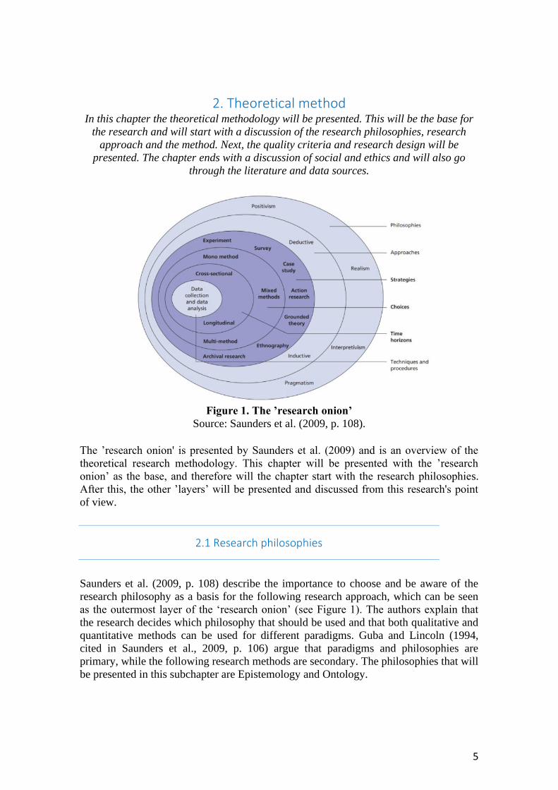
Figure 1. The ’research onion’

Source: Saunders et al. (2009, p. 108).

The ’research onion' is presented by Saunders et al. (2009) and is an overview of the

theoretical research methodology. This chapter will be presented with the ’research

onion’ as the base, and therefore will the chapter start with the research philosophies.

After this, the other ’layers’ will be presented and discussed from this research's point

of view.

2.1 Research philosophies

Saunders et al. (2009, p. 108) describe the importance to choose and be aware of the

research philosophy as a basis for the following research approach, which can be seen

as the outermost layer of the ‘research onion’ (see Figure 1). The authors explain that

the research decides which philosophy that should be used and that both qualitative and

quantitative methods can be used for different paradigms. Guba and Lincoln (1994,

cited in Saunders et al., 2009, p. 106) argue that paradigms and philosophies are

primary, while the following research methods are secondary. The philosophies that will

be presented in this subchapter are Epistemology and Ontology.

6

2.1.1 Epistemology Epistemology is described as one way to think about the different research philosophies

with the issue of whether knowledge should be accepted or not, and if the social world

should be studied the same way as the natural sciences (Bryman & Bell, 2011, p. 15).

Further on, the authors explain that epistemology can be divided into positivism and

interpretivism. If you follow a positivistic philosophy you work like a natural scientist

and will not present data if it doesn’t come from phenomena's that has been observed

(Saunders et al., 2009, p. 113). Positivism is connected to a deductive research approach

through its state that theory is used to generate hypothesis to be answered (Bryman &

Bell, 2011, p. 15). Thus, for this study a positivism point of view will be the approach

among epistemologies. This is since secondary historical data will be used and will be

presented only if it has been observed. As the data is published we can state that it is

observed and according to positivism it implies that the data can be presented.

The other perspective of epistemology, interpretivism, has a believe that humans and

institutions are separated from natural sciences (Bryman & Bell, 2011, p. 16). This

philosophy believes that physical sciences are not enough to explain the social world of

business (Bryman & Bell, 2011, p. 16). With an interpretivist view, as Saunder et al.

(2009, p. 116) explain, it is important to see people as different when conducting

information of human behaviour. As stated, our study will collect data from NASDAQ

Stockholm and Oslo Børs ASA the study will not adopt an interpretivist view, so the

epistemological point of view must be positivism since it states that only phenomena's

that has been observed can provide trustworthy data (Saunders et al., 2009, p. 119). For

a positivistic point of view, a quantitative data collection with big samples of data often

is used, with an independent approach from the researcher, which goes in line with the

purpose of this research.

2.1.2 Ontology Ontology seeks for explaining the social entities and the nature of reality (Saunders et

al., 2009, p. 110) and is another way to see the different philosophies. The main

question within ontology is if social units should be described as an objective

phenomenon to the actors in it or if the entities are a result of actions of the humans in it

(Bryman & Bell, 2011, p. 20). Objectivism and constructionism are two different

contrary approaches within the ontology consideration (Bryman & Bell, 2011, p. 20).

Objectivism states that social entities and phenomena are independent of social actors in

the social world (Bryman & Bell, 2011, p. 21), which implies that the social

phenomena’s people use every day, are separated from actors. Constructionism, or

subjectivism, on the other hand, has the opposite view of the social reality according to

the authors. With a constructionism view, the perceptions and actions of social actors

are the background to the social phenomena’s (Saunders et al., 2009, p. 111). It can

therefore be said that it’s the social actors in a social entity that shape it, not the

opposite, and the organisation is a product of social actors. Among ontology, this study

will therefore have an objectivistic point of view since the data that will be collected

from a stock exchange site where the data are not affected by the social actors.

Therefore, the data is separated and not subjective since the data should appear whether

there were social actors behind it or not.

7

2.2 Research Approach

The aim of this research is to evaluate if growth stocks outperform value stocks in the

Nordic countries by creating hypotheses and test them, which will be done by testing

theories on the markets of each countries. Therefore, our purpose is not to create new

theories, rather testing existing ones, which is best described by a deductive approach.

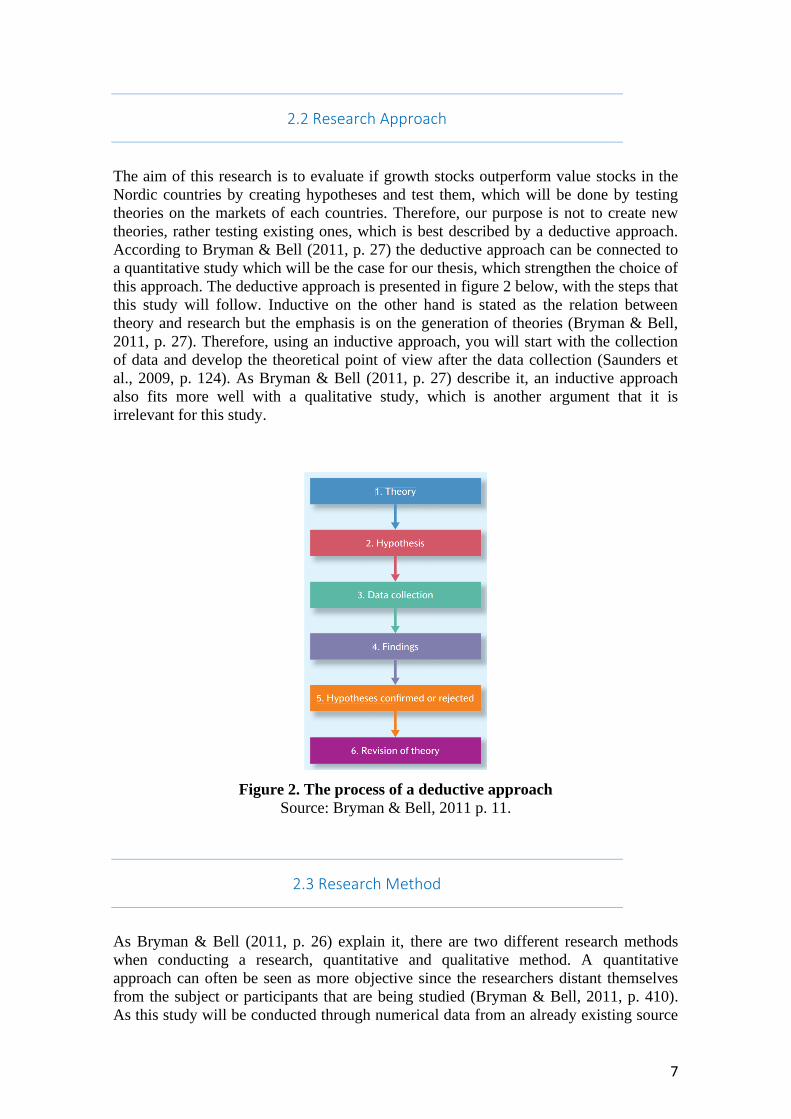
According to Bryman & Bell (2011, p. 27) the deductive approach can be connected to

a quantitative study which will be the case for our thesis, which strengthen the choice of

this approach. The deductive approach is presented in figure 2 below, with the steps that

this study will follow. Inductive on the other hand is stated as the relation between

theory and research but the emphasis is on the generation of theories (Bryman & Bell,

2011, p. 27). Therefore, using an inductive approach, you will start with the collection

of data and develop the theoretical point of view after the data collection (Saunders et

al., 2009, p. 124). As Bryman & Bell (2011, p. 27) describe it, an inductive approach

also fits more well with a qualitative study, which is another argument that it is

irrelevant for this study.

Figure 2. The process of a deductive approach

Source: Bryman & Bell, 2011 p. 11.

2.3 Research Method

As Bryman & Bell (2011, p. 26) explain it, there are two different research methods

when conducting a research, quantitative and qualitative method. A quantitative

approach can often be seen as more objective since the researchers distant themselves

from the subject or participants that are being studied (Bryman & Bell, 2011, p. 410).

As this study will be conducted through numerical data from an already existing source

8

the statement of a quantitative method will hold, and the objectivity will not be

compromised. Another argument for this type of study would be that it aims to test

theories in order to evaluate whether to reject or not reject a null hypothesis. The

qualitative approach focuses the data collection on words and the researcher tend to

seek involvement with the participants for a higher understanding (Bryman & Bell,

2011, p. 410). With all this information in mind we can reinforce our choice to conduct

a quantitative study over a qualitative, since the data collection will not have a focus of

subjective interpretations, nor that the study will have participants that improve the

understanding.

Even if there are many differences, we should also present some of the similarities

between the methods since these are also worth to bear in mind. One similarity is that

both methods are concerned with reduction of data, which is done for the purpose to

make sense of the data and be able to draw conclusions (Bryman & Bell, 2011, p. 412).

Further on, the authors explain that quantitative methods often use a statistical analysis

for this while qualitative develop concepts out of their data. Answering research

questions is another similarity, even if the method to do this is different; they both are

fundamentally concerned with answering questions regarding the nature of social reality

(Bryman & Bell, 2011, p. 412). However, it is the quantitative approach that this study

will follow.

2.4 Quality criteria

To determine and to evaluate research there are according to Bryman & Bell (2011, p.

41) three criteria: reliability, validity and replication. The criteria reliability shows

whether the result of a research is possible to repeat (Bryman & Bell, 2011, p. 41). If

that is the case, a variety of studies should present the same results. Further on, there are

three questions that can be used to measure the reliability “Will the measures yield the

same results on other occasions?”, “Will similar observations be reached by other

observers?” and “Is there transparency in how sense was made from the raw data?”

(Easterby-Smith et al. 2008:109, referred in Saunders et al., 2009, p. 156). Beyond these

questions, Bryman & Bell (2011, p. 157-158) highlight three criteria to evaluate if a

measure is reliable: stability, inter-observer consistency and internal reliability. Stability

shows if the measure is stable enough, or not stable, to promise that a result will be

stable over time. Inter-observer consistency concerns the possibility that the research

has subject impact of the study which can affect the choices. Internal reliability

measures if the factors that affects the indexes or scales of the research is consistent and

if the answers have coherence to give an overall score. These criterions among

reliability are important to consider for us in this thesis and will further be discussed in

the conclusions. Since using secondary data from Eikon, it is important for us during the

study to be transparent about how the data are collected and to be consistent about the

returns, indexes and ratios to be able to make the study reliable, and repeatable.

Validity can be described as a criterion that measures the relevance of the results of the

study, “whether the findings are really about what they appear to be about” (Saunders et

al., 2009, p. 157). One thing often referred to external validity is generalizability which

implies that the study needs to be able to be applied to other studies or for example

9

other organisations, even if it is different from the organisation in the chosen study

(Saunders et al., 2009, p. 158). As for reliability, validity will also be considered in this

study. When drawing conclusions and analysing the results, we will have in mind to

make sure that the results measure exactly what they should measure to assure that the

study is valid. As Bryman & Bell (2011, p. 159) states, there are several different ways

to measure validity and that there are different types of validity. Measurement validity

is most common for quantitative studies and measure in general if the measure of the

study or concept measure exactly what is supposed to measure (Bryman & Bell, 2011,

p. 42), which is very appropriate for this quantitative study and as stated above

especially important to have in mind. To reach this, we will maintain a critical point of

view to reduce the risk of drawing wrong conclusions when later analysing the results.

Further on there is internal validity which measure the causality of the measurements

(Bryman & Bell, 2011, p. 42). The authors explain the problem of causality as if there

are other thing that causes the relationship between, for example the parameters, X and

Y, and if we can be sure that the chosen variable is the only thing that affects the

relationship. External validity is also related to the issue of whether the conclusions of

the study can be applied to other studies (Bryman & Bell, 2011. p. 43), which is similar

to the problems that have been discussed above.

Since reliability and replication almost describe the same thing (Bryman & Bell, 2011,

p. 41), we will consider reliability and validity in this thesis, as reliability is even more

common than replication.

2.5 Time horizon

There are different research designs to consider when conducting research. Bryman &

Bell (2011, p. 45) uses five different types when they discuss these which include

experimental design, cross-sectional design, longitudinal design, the case study design

and the comparative design. Among the research designs there are also, according to

Saunders et al. (2009, p. 155), time horizons to consider when conducting a study. From

the five different designs mentioned above, the study should apply either a cross-

sectional or a longitudinal time horizon. The main difference between these is the length

of the time horizon: a cross-sectional is often used for qualitative studies when

conducting information over a short period of time while longitudinal studies is used

when you want to study change of a period (Saunders et al., 2009, p. 155). Further on,

the authors describe the main question of a longitudinal design as “Has there been any

change over a period of time?”. Since this study will compare different stocks over

different periods of times, the longitudinal design is applied to be able to answer the

research question. As stated, a cross-sectional is more often used in qualitative studies

and as this study aims to evaluate the historical data during 2021-2021 this time horizon

would not be possible to conduct.

10

2.6 Social & Ethical Research

Saunders et al. (2009, p.183-184) refers to ethic, in a research context, as how to behave

in an appropriate way in relation to the rights of the participants that will become a

subject of your work. This is related to how we clarify and formulate the research

design, topic, data collection and analysis of data and should therefore be both morally

and methodologically defensible (Saunders et al., 2009, p.183-184). To give some

examples of what can be included in research ethics, the importance of privacy and

consent of participants as well as anonymity can be highlighted, as well the data

collected which should maintain confidential. The researchers should also act

objectively and with a good behaviour (Saunders et al., 2009, p.185-186). Since our

data will be collected by using secondary data and not involve people, these problems

should not be a big issue for this study, thus it is important to have knowledge about

them. Though, it is important since it is, except for anonymity and confidentiality, about

how the data collection and analysis of the data is done. Even if we will not face a big

problem in terms of anonymity, as we might if a qualitative method would been used, it

is important that these steps are done with good morals and that we act objective during

the conduction of the study.

Bradford & Cullen (2011) present in their book that even if many ethics considerations

are connected to research involving human participants, there are those that needs to be

taken into consideration with secondary data as well. Secondary data includes

information collected by someone else and it is therefore important that the information

gathered there was collected ethically (Bradford & Cullen, 2011, p. 156-157). Another

thing to keep in mind when using secondary data is to clarify the purpose of the

information collected, due to the importance of using the data for the research purpose

and not mislead it from the original reason (Bryman & Bell, 2011, p. 139). By taking

this into consideration, we tend to provide the readers with a clear and visible data

collection method to do the research as ethically as possible.

2.7 Literature and Data Sources

According to Saunders et al. (2009, p. 69) the literature sources can be divided into

three categories which include primary, secondary and tertiary sources. The authors

mention that sources frequently intersect with one another and exemplify the fact that

books can contain indexes to primary literature. Primary literature can be referred to as

“grey literature” since it can be more difficult to trace because they are sources of the

first occurrence of a work (Saunders et al., 2009, p. 69). Some examples of primary

sources can include reports, government publications, letters etc. Secondary literature,

on the other hand, is the later publication of primary sources, for example reports and

books (Saunders et al., 2009, p. 69) Compared to primary literature, secondary is easier

to trace, and the publications target a broader audience. Lastly, the authors describe

tertiary literature as the source developed to help in the location of primary and

secondary sources, often referred to as “search tools”. Abstracts and dictionaries are

some examples of tertiary literature (Saunders et al., 2009, p. 69).

11

Secondary literature sources such as academic journals, books, and data from databases

are used in this thesis. The main parts of the sources used, are collected from Google

Scholar and Umeå University Library. We will also use the database Eikon, provided by

the University, to gather the necessary numerical data, and Microsoft Excel to analyse

it. Since secondary literature will cover the main part of the data collection in this study, it

is important to highlight and evaluate the pros and cons of this type of source. Bryman

& Bell (2011) present some of the advantages and limitation for this method. First, it is

cost effective and time saving to use due to the easy access to good-quality data

(Bryman & Bell, 2011, p. 313). Although, by using already existing data, these can be

more complex to understand since the researcher lack familiarity with the structure and

contour of the data. Thus, since it is time saving, this provides the researcher with more

time to analyse and understand the data (Bryman & Bell, 2011, p. 320). Another

limitation worth mentioning is the difficulty to control the quality of the data collected.

However, by using peer-viewed sources, which can be considered as reliable, this

disadvantage could be minimized to avoid biases or mistakes (Bryman and Bell, 2011,

p. 321).

2.8 Source criticism

According to Bertilsson (2021, p. 2) it is of great importance to be critical towards the

gathering of information from different sources and data to avoid spreading wrongful

information. Bertilsson (2021, p. 2) explains that there are four main criteria of source

criticism: authenticity, time, dependency and tendency. By evaluating these criteria, we

can determine the trustworthy and credibility of the information. Further on, the author

refers authenticity to the importance of validating who the authors of the information

might be or where the original source comes from. To fulfil this criterion it is important,

during the work with this research, to locate the primary sources. If that’s not possible at

some time, it is then important to refer to the original source and validate the second

source. This goes hand in hand with dependency, which describes the connection

between different sources and whether one source relies on or repeats another source

(Bertilsson, 2021, p. 2). If there might be potential bias from the author’s side, this is

the criteria of tendency. This includes that the authors need to inspect the information

before including the data, to see if there could be personal, political or economic biases

from the source, which also is of great importance to consider along the work with this

research to fulfil that the sources remain objective. The last criteria to consider is time,

information or sources that are closer in time are often, but not necessary, more

trustworthy (Bertilsson, 2021, p.2).

12

2.9 Summary of the theoretical methodology

Table 1: Summary of the theoretical methodology Epistemological position Positivism

Ontological position Objectivism

Research approach Deductive

Research method Quantitative

Research design Longitudinal design

To give an overview of the theoretical methodology used in this study, this chapter will

end with a summary, table 1. Concerning the research philosophies, a positivistic point

of view will present the epistemological position since only empirical results will be

accepted. An objectivistic position for the ontological position equals the fact that

human factors will not impact the results since it will have a view of reality which is

external from the human factors within it. Further on, a deductive approach will be used

since hypothesis will be designed from previous theories, and not the contrary. The

research method is quantitative as the empirical that will be used is secondary data.

Lastly, a longitudinal design is used for the time horizon.

13

3. Theoretical point of departure This chapter will discuss and explain the different theories that are connected to the

research question. It starts with a presentation of the choice of topic, then previous

research that is relevant for growth and value stocks are presented. Further on,

different financial models and theories will be presented.

3.1 Choice of topic

Both authors of this thesis are finishing their last semester of Master of Science in

Business and Economics. The choice of finance, and more exactly investments as the

main subject for the thesis came both from out personal interests in investing in the

stock market and because of the academic background of studies in business and

finance. At first, our thought was to conduct the research on the Swedish stock market,

since the Swedish stock market felt extra interesting as we both have invested in

different types of securities, stocks and funds on the Swedish stock market. However,

the more we read about the subject, we found already relevant research on the stock

market in Sweden, even if it was not as extensive as for the rest of Europe and US. We

then found that there was a research gap among the other Nordic countries and that

developed the idea to do a comparison between Sweden and Norway among value and

growth stocks. The fact that periods of financial distress only have been touched upon,

led us to the focus of financial crisis and to develop that area among value and growth

stocks. Lastly, to bring a wider knowledge about investment strategies in times of

financial distress.

The academic background within business, economics and master courses in finance

gave us a background and knowledge we needed to write this thesis since we are

already familiar with some of the theoretical parts, models and ratios. We are though

aware that the pre-knowledge can have an impact on the work, which we will take into

consideration and have in mind through the thesis to remain objective.

3.2 Growth versus value stocks

Since the study aims to investigate if a portfolio of growth stocks provides a higher

return than value stocks, the theoretical framework will start with an introduction of

growth and value stocks and how to distinguish these. Discussing differences between

value and growth stocks are important to provide the reader with basic knowledge

before several models and previous research among the topic will be presented.

As already stated, the price-to-earnings (P/E) ratio will be used to determine whether a

stock is defined as a value or a growth stock. As the name of the ratio implies, it is a

multiple that compares the share price with the earnings. More exactly, it equals the

price of the share divided by the earnings per share and tells us how much an investor of

the stock needs to pay for the earnings the company generates. It is also generally said

14

that the P/E ratio shows the markets expectations of future earnings. A high (low) P/E

ratio is because of that a sign that the market predicts that the earnings will be higher

(lower) in the future (Penman, 2010, p 49). Though, according to previous studies it can

be difficult to use ratios to categorize a stock into growth or value stocks. Schiessl

(2014) is one of the researchers who exemplify the difficulty of classification. The fact

that the ratios can change over time is one example given (Schiessl, 2014, p. 6). Another

difficulty is that both growth and value managers sometimes invest in the same

company (I.e., with the same ratio) even if they have different perceptions about it.

However, the P/E ratio will still be the categorization tool that will be used to

distinguish between value and growth stocks since it is one of the most common due to

previous studies (Basu, 1977; Schiessl, 2014).

Schiessl (2014, p. 4) described growth stocks as stocks that has an expectation of

making high earnings in the future with a growth rate higher than the average market,

which is synonymous with the explanation of a high P/E ratio. It can be explained that

the investors who invests in growth stocks has a belief that the company will

outperform the market both in the future and in the long run (Schiessl, 2014, p. 4-5).

Investors are therefore willing to pay more for a growth stock compared to value stocks.

The expectations about future earnings and growth are then high which indicate that if

these are correct, investing in a growth stock will be a good choice with increasing

stock prices as a result. Opposite, there is a risk in investing in growth stocks with a

declining stock price if the expectations are not fulfilled (Schiessl, 2014, p 5). Value

stocks, on the other hand, are often described as a firm with a past performance of not

providing as good results as growth stocks. Value stocks are often predicted to perform

below average (Schiessl, 2014). These, in contrast to growth stocks, often provide low

ratios such as P/E and high dividend yields (Schiessl, 2014, p. 1).

Chan & Chen (1991, cited in Jensen et al., 1997) stated that value stocks also can be

risky in terms of small firms and low ratios since there is a possibility that the firm

would not survive in periods of decline compared to bigger firms with high ratios. This

can have impacts on how the stocks perform during a financial crisis. Also, as Schiessl

(2014, p. 5) states, there is a risk that value stocks are traded under its true value

because of poor management. However, as mentioned in the first chapter, the

performance of value and growth stocks can among other things, depend on how high

the repo rate is. With a rising repo rate, the value stocks often present a higher return

since the performance of growth stocks are dependent of predicted future cash flows

and expected returns (Bratt, 2021). Further on, Bratt (2021) explains the expected cash

flows and returns are harder to predict when the rate is higher and this can be a cause of

low returns for growth stocks during times with high rates, since the growth stocks are

depending on future expected returns and cash flows. Thus, value stocks often present a

higher return during times of low rates. The Swedish Central Bank has provided

negative repo rates for most of the years the last decade, and 1.5 % at most (Sveriges

Riksbank, n.d.). Thus, the last decade has consisted of historical low rates, compared to

the 2000’s. In the previous decade (2000-2010) the rate was between 0.25 % and 4.5 %

on a quarterly basis (Sverige Riksbank, 2022). The same pattern is shown for the rate in

Norway, even if it has not been negative. During 2000-2010 the Norwegian policy rate

were between 1.25 and 7.00 % (Norges bank, n.d.) and after 2010 between 0.00 % and

2.5 %.

15

Besides the discussion of P/E ratio above, there is a concept that one can connect to this

measurement which is called P/E effect. We want to mention this since it is a concept

within finance that can provide an idea on how the P/E ratio can be used and the

outcome from its result. The P/E effect has been investigated in several studies. Basu

(1977) is one of the first findings of the research among the P/E ratio and he wanted to

investigate if there was empirical evidence that stocks are related to the P/E ratios. He

found, after dividing portfolios into percentiles based on the P/E ratios, that low P/E

ratios presented a higher return than these with high P/E ratios. These results go against

the Efficient market hypothesis and a semi strong form of market efficiency. However,

after Basu (1977) conducted his study there have been many researchers investigating

value and growth stocks and the P/E ratio with contrary results, which will be further

discussed in coming sub-chapters.

3.3 Fama & French Factor Models

To explain the fact that distressed (value) firms historically outperformed overvalued

(growth) firms, even if the growth firms have higher earnings, Fama & French (1993)

developed a three-factor model. Even though this model does not take the P/E ratio in

consideration, it is interesting to bring up since it gives a background for the discussion

of value and growth stocks. It also gives a background for the previous success for

value stocks and the P/E effect since more recent studies has showed contrary results.

Another reason of the relevance for Fama & French in connection to our study is since

it is a contrary model to what we are trying to investigate. Fama & French is based on

the statement that value tends to outperform growth companies and it will be interesting

to test if our result will go against this or not. By that we mean if growth stocks can

outperform value stocks. However, our intention will not be to investigate how our

result will present in comparison to the Fama & French model, rather provide an

alternative insight beyond the methods and financial measurement this study will focus

on.

The factors in the Fama & French model are size, excess return on the market and

value, which is specified as book-to-market values. According to Fama & French (1998,

p 1975) a capital asset pricing model were not enough to explain the value premium for

value stocks, and therefore they added size and value to their model. Fama & French

(1998, p. 1975) explains that value stocks outperformed growth stocks with an average

of 7.68 percent a year, in terms of firms with low versus high price to book ratios over

the years 1975-1995, and therefore they added size and value to their model.

Over the years it has been a discussion about whether this model is explained by market

efficiency or market inefficiency (Hayes, 2021). If the factor-model is explained by

market efficiency the higher return of the value stocks depends on the higher risk that

value stocks bring due to their bigger business risk and the higher cost of capital. The

supporters of market inefficiency instead hold on to the fact that the higher return is a

result of incorrectly pricing the value companies, which in turn leads to a greater return

among the way that the value adjusts (Hayes, 2021).

16

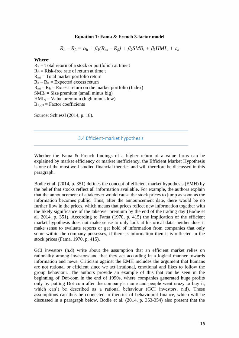
Equation 1: Fama & French 3-factor model

Rit – Rft = αit + β1(Rmt – Rft) + β2SMBt + β3HMLt + εit

Where:

Rit = Total return of a stock or portfolio i at time t

Rft = Risk-free rate of return at time t

Rmt = Total market portfolio return

Rit – Rft = Expected excess return

Rmt – Rft = Excess return on the market portfolio (Index)

SMBt = Size premium (small minus big)

HMLt = Value premium (high minus low)

Β1,2,3 = Factor coefficients

Source: Schiessl (2014, p. 18).

3.4 Efficient-market hypothesis

Whether the Fama & French findings of a higher return of a value firms can be

explained by market efficiency or market inefficiency, the Efficient Market Hypothesis

is one of the most well-studied financial theories and will therefore be discussed in this

paragraph. Bodie et al. (2014, p. 351) defines the concept of efficient market hypothesis (EMH) by

the belief that stocks reflect all information available. For example, the authors explain

that the announcement of a takeover would cause the stock prices to jump as soon as the

information becomes public. Thus, after the announcement date, there would be no

further flow in the prices, which means that prices reflect new information together with

the likely significance of the takeover premium by the end of the trading day (Bodie et

al. 2014, p. 351). According to Fama (1970, p. 415) the implication of the efficient

market hypothesis does not make sense to only look at historical data, neither does it

make sense to evaluate reports or get hold of information from companies that only

some within the company possesses, if there is information then it is reflected in the

stock prices (Fama, 1970, p. 415).

GCI investors (n.d) write about the assumption that an efficient market relies on

rationality among investors and that they act according in a logical manner towards

information and news. Criticism against the EMH includes the argument that humans

are not rational or efficient since we act irrational, emotional and likes to follow the

group behaviour. The authors provide an example of this that can be seen in the

beginning of Dot-com in the end of 1990s, where companies generated huge profits

only by putting Dot com after the company’s name and people went crazy to buy it,

which can’t be described as a rational behaviour (GCI investors, n.d). These

assumptions can thus be connected to theories of behavioural finance, which will be

discussed in a paragraph below. Bodie et al. (2014, p. 353-354) also present that the

17

implications are described more detailed in the three forms of market efficiency that

Fama created: weak, semi-strong and strong form.

3.4.1 Weak form According to Bodie et al. (2014, p 353) a weak form indicates that stock prices already

reflect the past information available that can be gathered by evaluating the history of

previous stock prices, short interest or volume. Past stock price data is freely available

and can be obtained at a small fee. The authors point out that the weak-form hypothesis,

if such data ever provided trustworthy signals about future performance, all investors

would have figured out how to profit from them by now. The prices of stocks would

instantly increase as the signals became more officially known, thus, a buy signal

should reduce the value. Therefore, according to this version of the theory, trend

analysis is useless (Bodie et al., 2014, p. 353).

3.4.2 Semi-strong form In a book written by Szylar (2013, p. 32) the semi-strong form means that publicly

available information concerning a company is already reflected in the stock prices. The

semi-strong form may appeal to our common sense the most and is therefore closer to

reality. It states that when significant new information is published, the market will

quickly absorb it by adjusting the price to a new equilibrium level that represents the

shift in supply and demand produced by the information's appearance. Szylar (2013, p.

32) states the semi-strong EMH makes up for its lack of intellectual rigor with empirical

strength, as it is easier to test than the strong EMH. One issue with the semi-strong

EMH is determining what constitutes "relevant publicly available information." As

appealing as the statement may appear, the reality is less so, because information does

not come with a handy label indicating which shares it affects and which it does not

(Szylar, 2013, p. 32).

3.4.3 Strong form Lastly, the strong hypothesis states that private information available within a company

as well as all relevant information connected to the firm is already reflected in the stock

prices (Bodie et al. 2014, p.354). An example of the strong form of market efficiency is

presented by Szylar (2013, p. 31). His example states that if one person possesses

confidential information and believe that the current market price is not justified to the

real value, the holders of that information will acquire the shares to take advantage of

the pricing anomaly. The holders of the classified information will keep acquire shares

until the oversupply of shares has pushed the price up to the level supported by their

classified information. They will have little motivation to keep buying at this point, so

they will exit the market, and the price will settle at this new equilibrium level (Szylar,

2013, p. 31).

EMH is a relevant theoretical framework to mention in this thesis since it would imply

that none of the stock portfolios should generate any major profits, if the EMH is to be

true. This is because the future gains from these stocks should be factored into the stock

prices. In other words, there should be no meaningful risk-adjusted returns. Thus, by

including this concept in the study we let the reader gain understanding of the theories

that propose a value premium cannot exist and why it cannot exist.

18

3.5 Random walk theory

The Efficient market hypothesis is evolved from previous theories and the random walk

theory is one of them (Kendall, 1953, p.13), which make this theory an important

background to understand the other theories that are presented. According to Mishkin

(2010) the random walk theory is an investment concept which assumes that the market

prices move up and down without following a certain pattern, with no power from

previous price fluctuations. With background of this, it is then impossible to predict

which way the market will go regardless of time. Keane (1983, cited in Chitenderu et

al., 2014, p. 1243) explains that the random walk theory argues that the direction a stock

price takes are random and can therefore not be forecasted based on previous price data.

According to the investors who agree with the RWT, they cannot outperform the market

without taking on greater risk. As a result, attempting to apply the theories will be a

waste of effort with no further benefits (Keane, 1983, cited in Chitenderu et al., 2014, p.

1243). Further on, Eugene F. Fama is one of the most influential researchers within the

area of random walk theory and has tested the theory a various amount of time. It could

be determined that there is no dependence in stock price series that can be considered as

important for investment purpose, which means that history can’t be used to increase

the investors expected profit (Fama, 1965, p. 87).

However, there are studies that talks both for and against the RWT. Van Horne &

Parker (1967) did a study consisting of industrial stock on the New York stock

exchange and wanted to test empirically the RWT in relation to past stock price

movements. They concluded that their study did support the random walk theory and

that trades who relied on past stock prices did not gain greater profits than buy-and-hold

investors (Van Horne & Parker, 1967). A study made by Hang & Grochevaia (2015)

tested to see if the Shanghai and Shenzhen markets, which are the most influential stock

markets in China, followed a random walk from 1992-2015. The overall result of this

thesis was that the return contradicted the random walk theory and that a pattern based

on the whole time period could be seen. Though, they also performed test on sub-

periods within the two markets which provided some inconsistency against the

statement to reject the null hypothesis of a random walk (Hang & Grochevaia, 2015, p.

29).

Worthington & Higgs (2004) performed a study which was made by looking at 20

markets in Europe. Their result provided evidence that most of the countries did not

meet the criteria for the random walk and its behaviour. Along with this study, more

research on the same theory is made which also proved to be against the random walk,

this result in difficulties to draw any conclusions about the RWT since the studies used

the same methods yet showed different results. Though, the authors explain that this of

course can depend on other factors, such as the economic situation during the tested

time-period, efficiency of the market or level of development in the researched country

but this is a subject for a future thesis (Worthington & Higgs, 2004). The random walk

theory is a core concept within the subject of finance that we have decided to conduct

this research on. Even if this theory wouldn’t be the main focus for us to test, it is

relevant to present since it is well connected to the efficient market hypothesis, which is

a theory that we will discuss later in the thesis. Both of these theories main statement is

19

that it is impossible to outperform and predict the market which is important to know in

order to gain a better understanding of the patterns of in the stock market.

3.6 Behavioural finance

According to several economists there are doubts on the precision of the Efficient

Market Hypothesis and the Random walk theories. Instead, they put their focus on the

concept of behavioural finance. Some of the arguments on this are that humans are not

logical in nature, and this is ignored in the Efficient Market Hypothesis (Bodie et al,

2014, p. 389). Therefore, theories of behavioural finance add further knowledge and

criticism against the previous theories brought up in this chapter.

Behavioural finance is a quite new concept within finance and has its roots from

behavioural economics, conventional finance and psychology. Discover biases, defects

and irrationalities in human decision-making can be said to be the main goal when it

comes to financial issues (Brealey et al., 2017, p. 340). Therefore, it is important to

recommend solutions and address them so that better decisions can be made. The

authors also describe that biases in behavioural finance may be due to individuals'

attitudes towards their own investing strategies. Conservatism is one of them, which

indicate that investors take too much time in the adjustment of their portfolios and

investment strategies when they are faced with new information (Brealey et al., 2017, p.

340). They tend to react in a correct way, though, to a less extent than would be

required (Brealey et al., 2017, p. 340). The other bias worth mentioning in terms of

behavioural finance is that some investors tend to be too overconfident in their

investment strategies which may attribute consequences to external causes or simply

bad luck (Brealey et al., 2017, p. 341).

Behavioural finance enables investors to gain a deeper understanding to the drivers of

their own, and their clients’ decision and apply this knowledge in their professional

practice to make better and more rational decisions (Valsova, 2016). In an article

written by Olsen (2008, p. 3) he states that people tend to connect larger groups with

comfort, which is also seen in finance. This can be referred to as herd instinct, and to

apply this into investment decisions we could say that a larger group can indicate a

lower risk. A positive affect from being associated as a member of a group also tend to

make us look past our own feelings and instead go with the group. Investors that follow

this behaviour can ignore their own forecasts and investment decisions in order to

follow the “reference group,” which may include other market participants, friends or

colleagues (Olsen, 2008, p. 3).

According to Ritter (2003, p.429) behavioural finance is founded on psychology, which

claims that human decision-making is prone to a variety of cognitive illusions. The

illusions can be divided into two categories. The first category, heuristic, can be defined

as “the rules of thumb.” This simplifies the decision-making, particularly in complicated

and uncertain situations (Ritter, 2003, p.431). This is done by reducing the complexity

of evaluating probability and forecasts to easier judgments (Kahneman & Tversky,

1974, p.1124). The heuristic concept is often useful, especially when time is short,

although they can lead to biases (Kahneman & Tversky, 1974, p.1124-1131). The

second category, prospect theory, can be defined as the concept where gains and losses

20

are valued differently. This will result in making decisions based on supposed rewards

rather than losses (Kahneman & Tversky, 1979, p.263). There is also evidence showing

that behavioural finance affects the price-volatility of securities. Olsen (1998) stated

that higher behavioural effects, intuitive decision procedures and stress, will result in

higher volatility. Further on, higher volatility can be a factor of poorly structured

decisions since the outcome can have higher unpredictability of decisions, bigger

differences of prices and a difficulty to measure returns. One reason of why we have

decided to present the behavioural finance theory is because it can be useful to have in

mind when discussing our results. The stock market is built on investors with different

behaviours and it will be interesting to evaluate if any pattern can be seen in terms of

behaviour, group pressure and irrationality.

3.7 Modern portfolio theory

Modern portfolio theory hold the same assumptions as the Efficient market hypothesis

and describes the fact that an investor can’t beat the market on a risk adjusted basis by

evaluating past prices. This theory can also be described as a theory that goes against

Behavioural finance, as it assume rational and risk adverse investors with no abnormal

risk adjusted returns. How to maximize the return for a given level of risk or decrease

risk for a given level of return can be described by the modern portfolio theory

(Markowitz, 1952). The theory states that the adaption of risk and return is done by

diversification, with intention to reduce unsystematic risk that investors may face when

owning one or few highly correlated stocks (Markowitz 1952, p.89).

To produce the best set of portfolios in theory, Markowitz (1959) created a

mathematical procedure for this. Investors could develop a table based on portfolios

with the same level of risk, where the risks are the same, but the returns differ, which

would indicate that the portfolio with the highest return is simply the best due to the

same risk level (Markowitz, 1959). The key to a reduction in risk is the correlation

between the stocks. This means that if a sector or a firm receives negative news, the

price of the stock in the portfolio will decrease. It would then lead to a fall in the stock

price of another highly related stock in the portfolio.

A study by Kierkegaard et al. (2006) investigated if investors can apply the MPT to

achieve a higher return than investing in an index. They concluded that the optimal

risky portfolio did provide a higher return than a passive index, during the five years the

study covered. The authors, on the other hand, are hesitant to conclude that investing

according to MPT, based solely on historical data and would be a preferable option to

an index portfolio (Kierkegaard et al., 2006, p. 35). In the context of this thesis, the idea

of distinguishing stocks that earn an abnormal risk adjusted return goes against MPT's

ideas. One reason why we decided to include the MPT in our thesis is because one of

the disadvantages of this theory is that it assumes that investors are rational and aim to

increase the return while reducing risk. However, as described in 3.6, investors tend to

act irrational and often end up following the groups behaviour which will be a limitation

for this theory. It will be interesting to see if we can draw any conclusions of

irrationality among investors based on our result.

21

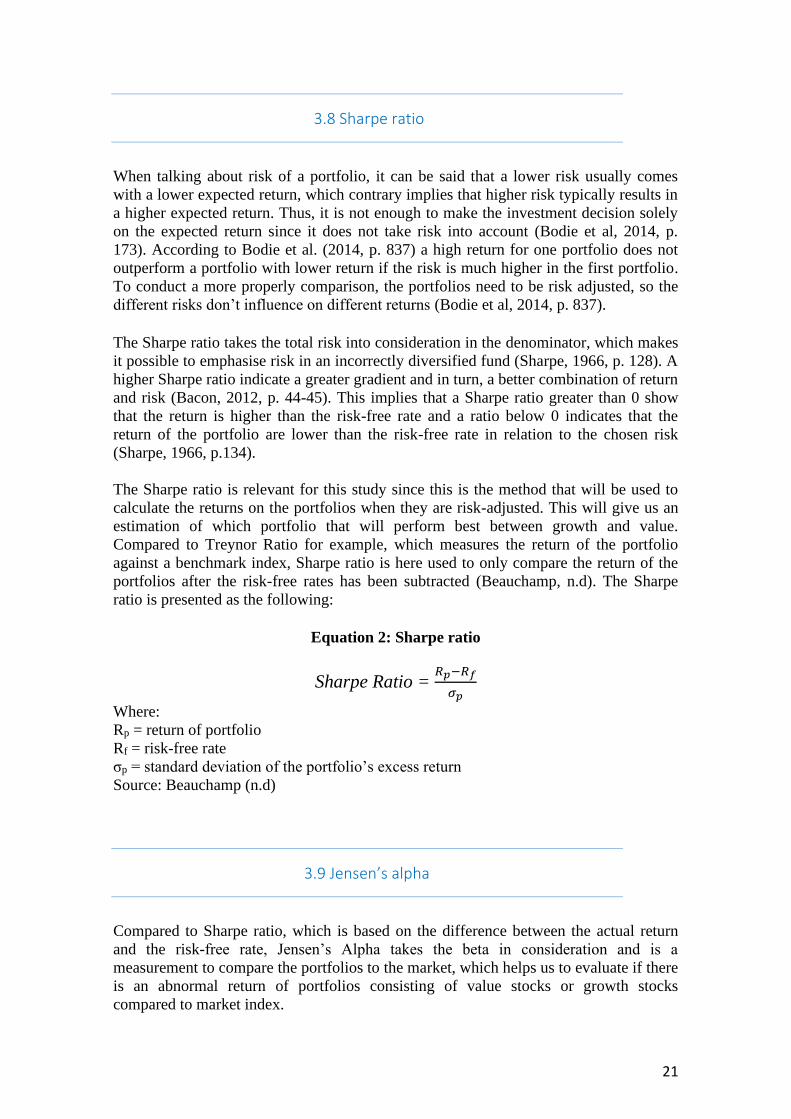
3.8 Sharpe ratio

When talking about risk of a portfolio, it can be said that a lower risk usually comes

with a lower expected return, which contrary implies that higher risk typically results in

a higher expected return. Thus, it is not enough to make the investment decision solely

on the expected return since it does not take risk into account (Bodie et al, 2014, p.

173). According to Bodie et al. (2014, p. 837) a high return for one portfolio does not

outperform a portfolio with lower return if the risk is much higher in the first portfolio.

To conduct a more properly comparison, the portfolios need to be risk adjusted, so the

different risks don’t influence on different returns (Bodie et al, 2014, p. 837).

The Sharpe ratio takes the total risk into consideration in the denominator, which makes

it possible to emphasise risk in an incorrectly diversified fund (Sharpe, 1966, p. 128). A

higher Sharpe ratio indicate a greater gradient and in turn, a better combination of return

and risk (Bacon, 2012, p. 44-45). This implies that a Sharpe ratio greater than 0 show

that the return is higher than the risk-free rate and a ratio below 0 indicates that the

return of the portfolio are lower than the risk-free rate in relation to the chosen risk

(Sharpe, 1966, p.134).

The Sharpe ratio is relevant for this study since this is the method that will be used to

calculate the returns on the portfolios when they are risk-adjusted. This will give us an

estimation of which portfolio that will perform best between growth and value.

Compared to Treynor Ratio for example, which measures the return of the portfolio

against a benchmark index, Sharpe ratio is here used to only compare the return of the

portfolios after the risk-free rates has been subtracted (Beauchamp, n.d). The Sharpe

ratio is presented as the following:

Equation 2: Sharpe ratio

Sharpe Ratio = 𝑅𝑝−𝑅𝑓

𝜎𝑝

Where:

Rp = return of portfolio

Rf = risk-free rate

σp = standard deviation of the portfolio’s excess return Source: Beauchamp (n.d)

3.9 Jensen’s alpha

Compared to Sharpe ratio, which is based on the difference between the actual return

and the risk-free rate, Jensen’s Alpha takes the beta in consideration and is a

measurement to compare the portfolios to the market, which helps us to evaluate if there

is an abnormal return of portfolios consisting of value stocks or growth stocks

compared to market index.

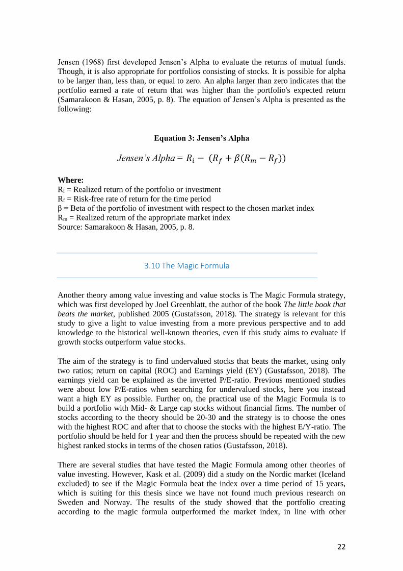
22

Jensen (1968) first developed Jensen’s Alpha to evaluate the returns of mutual funds.

Though, it is also appropriate for portfolios consisting of stocks. It is possible for alpha

to be larger than, less than, or equal to zero. An alpha larger than zero indicates that the

portfolio earned a rate of return that was higher than the portfolio's expected return

(Samarakoon & Hasan, 2005, p. 8). The equation of Jensen’s Alpha is presented as the

following:

Equation 3: Jensen’s Alpha

Jensen’s Alpha = 𝑅𝑖 − (𝑅𝑓 + 𝛽(𝑅𝑚 − 𝑅𝑓))

Where:

Ri = Realized return of the portfolio or investment

Rf = Risk-free rate of return for the time period

β = Beta of the portfolio of investment with respect to the chosen market index

Rm = Realized return of the appropriate market index Source: Samarakoon & Hasan, 2005, p. 8.

3.10 The Magic Formula

Another theory among value investing and value stocks is The Magic Formula strategy,

which was first developed by Joel Greenblatt, the author of the book The little book that

beats the market, published 2005 (Gustafsson, 2018). The strategy is relevant for this

study to give a light to value investing from a more previous perspective and to add

knowledge to the historical well-known theories, even if this study aims to evaluate if

growth stocks outperform value stocks.

The aim of the strategy is to find undervalued stocks that beats the market, using only

two ratios; return on capital (ROC) and Earnings yield (EY) (Gustafsson, 2018). The

earnings yield can be explained as the inverted P/E-ratio. Previous mentioned studies

were about low P/E-ratios when searching for undervalued stocks, here you instead

want a high EY as possible. Further on, the practical use of the Magic Formula is to

build a portfolio with Mid- & Large cap stocks without financial firms. The number of

stocks according to the theory should be 20-30 and the strategy is to choose the ones

with the highest ROC and after that to choose the stocks with the highest E/Y-ratio. The

portfolio should be held for 1 year and then the process should be repeated with the new

highest ranked stocks in terms of the chosen ratios (Gustafsson, 2018).

There are several studies that have tested the Magic Formula among other theories of

value investing. However, Kask et al. (2009) did a study on the Nordic market (Iceland

excluded) to see if the Magic Formula beat the index over a time period of 15 years,

which is suiting for this thesis since we have not found much previous research on

Sweden and Norway. The results of the study showed that the portfolio creating

according to the magic formula outperformed the market index, in line with other

23

studies on the US market. A study of Brindelid & Nilsson (2021) also showed that the

created portfolios with the Magic formula theory generated excess return compared to

market indexes during the period 2012-2021 for all the Nordic countries (Iceland

excluded). Though, it showed that the strategy led to even higher returns in Norway

compared to Sweden.

3.11 Additional research

It is earlier mentioned that previous research covering the area, whether value or growth

stocks provide a higher return, has already been made, but with the focus on US, Europe

and a few on smaller markets such as the Swedish market. Thus, we have not found that

much research concerning the Norwegian market, neither a comparison between

Sweden and Norway and how they are in relation to each other when it comes to growth

and value stocks. However, in this section some more previous studies related to our

research will be presented.

Sharpe et al (1993) found that value stocks outperformed growth stocks during the

period 1981 and 1992. The researchers found that value stocks, based on the price-to-

book (P/B) ratio outperformed growth stocks (Sharpe et al., 1993, p. 27). They had

evidence for this both for the actual returns and the risk-adjusted returns but however

clarified that previous studies have shown that the returns have differed a lot from year

to year and month to month, and so on. Fama & French (1998) also found similar

results. They found that value stocks before 1998 performed better with higher returns

than growth stocks. An explanation to that were according to the authors a correction

after an undervaluation of the value stocks, while the growth stocks were overvalued.

Gregory et al. (2003, p. 213-255) conducted a study between 1980 to 1998 on stocks on

the New York stock exchange. They wanted to test if value stock outperformed growth

stocks due to a higher risk level for the value stocks. They concluded that value stock

portfolios were not riskier, but still outperformed growth stocks portfolios. To divide

the stocks into value or growth stocks, they used ratios such as earnings-to-price (EP),

cash-flow-to-price (CP), book-to-market (BM) and sales growth to differentiate these. Another study performed within this subject of value and growth stocks was presented

by Gharghoria et al. (2013, p. 393-417). This paper was based on the Australian market

and wanted to investigate if there is a value-growth effect on the market, as well as

identify which accounting ratio could describe this in the most accurate way. The result

in this research, same as the previous mentioned, showed that value stocks performed

better than growth stocks, it also implied that the best ratio to use in the evaluation of

performance was book-to-market alongside with cash flow-to price. They divided their

portfolios based on book-to-market (B/M), sales-to-price (S/P), debt-to-equity (D/E),

firm size, positive earnings-to-price (E/P+), negative earnings-to-price (E/P)), positive

cash flow-to-price (C/P+) and negative cash flow-to-price (C/P).

A study made by Vorwerg (2015) was based on the German stock market between

2005-2014. The purpose was to investigate if a portfolio including value stocks would

outperform a portfolio based on growth stocks. The conclusion from this thesis is

supporting the ones above, that value stocks outperformed growth stocks. Thus, it is

24

only valid for the P/CF multiplier. The study also mention that the study can be biased

since it was conducted during the global financial crisis and European debt crisis which

could have a possible effect on the results. As a further research suggestion, it said to

increase the timeframe to cover a larger span to get more valid results (Vorwerg, 2015).

He performed the study based on the measurements price-to earnings (P/E), price-to-

book (P/B), price-to-cash-flow (P/CF). Van Dinh (2021) conducted a study from

Helsinki stock exchange between the years 2015-2019 which aimed to evaluate the

performance of value stocks versus growth stocks. Holding periods for the study was 6

months and the comparison was on the average annual returns and risk-adjusted returns.

The study showed that a contrarian investment strategy in value stocks were not likely

to yield a higher risk-adjusted return than growth stocks (Van Dinh, 2021).

3.12 Summary of theoretical framework

As stated, the main purpose of this research is to investigate whether a portfolio

consisting of growth stocks (high P/E ratio) would outperform a portfolio of value

stocks (low P/E ratio) and make a comparison between Norway and Sweden to see if

any clear difference can be seen. Previous studies mentioned in this chapter often

support the finding that value stocks tend to outperform growth stocks. Though,

research from the last decade has showed contrary results and points out that high P/E

stocks sometimes outperform low P/E stocks. To give an introduction to the value and

growth stocks, the chapter started with a description of these, along with the

characteristics they tend to be connected to.

The main theories presented were Efficient Market Hypothesis, the random walk theory

and the modern portfolio theory. Similar assumptions are hold for the Efficient market

hypothesis as well for the Random walk theory. This is since these theories state that

beating the market is impossible since the market is always entirely informed which in

turn reflects the prices, which will be investigated. If the Efficient market hypothesis

would be true, high P/E stocks should not outperform low P/E stocks. Modern Portfolio

Theory clarifies how diversification of a portfolio can improve expected returns as well

as reduce the risk. In the context of this thesis, the idea of identifying undervalued

stocks that earn an abnormal risk adjusted return goes against Modern portfolio theories

ideas and the risk-to-reward ratios on which it is based. To evaluate the theories the

risk-adjusted returns are tested through Sharpe ratio along with Jensen’s alpha which

takes the market indexes in consideration to make it possible to investigate how the

portfolios perform compared to market.

As a contrary theory to these theories, Behavioural finance is discussed to give idea on

how psychology can be connected to investing. Followers of theories among

behavioural finance in turn state that humans are not rational as we have a tendency to

follow groups and that human decisions can lead to higher volatility in stock prices and

a difficulty to measure returns. Thus, we can state that these assumptions go against the

theories discussed above, which all have an assumption of rational behaviours and these

theories will be interesting to evaluate after the study have been conducted. Among the

different studies and theories that have been discussed, the magic formula is also

brought up to give another light to the different investment strategies. Researchers who

25

followed the magic formula have showed that portfolios created according to this

strategy have outperformed market indexes in the most cases, which also will be

compared to the results this study conducts.

26

4. Practical method

This chapter will explain the practical method used to collect and analyse the data to be

able to answer the research question of the study. Since a quantitative method is used,

there will be several tables and statistical models presented.

4.1 Data collection

The data for this thesis will be gathered from the data system Eikon from where the

stock prices will be downloaded to calculate the yearly returns. The same will be done

for the market index returns. We will later use and evaluate these in our empirical

findings to provide an answer to the research question and to test our hypotheses. The

P/E ratios will also be gathered from Eikon which will be used in the classification of

value versus growth stocks. After the stocks have been collected with the P/E ratios, the

portfolios allocation will be made in Microsoft Excel.

Our sample data will consist of companies listed on the stock markets of Sweden and

Norway; NASDAQ Stockholm and Oslo Børs ASA. Further on, data will also be

collected from the indexes Olso All Share (OSEAX) and Stockholm OMXPI, since the

portfolios also will be compared to market index.

4.1.1 Sample selection and Creation of portfolios Since the purpose of the thesis is to compare the performance and returns of value

versus growth stocks, these need to be divided into separate portfolios. This will be

done based on the years between 2001-2021, including four sub-periods during which

will also be compared and discussed. To implement this, the portfolios will be

constructed based on low and high P/E ratios to identify if they are classified as value or

growth stocks. All raw data will be provided from Eikon Datastream.

The portfolio of value stocks will include the 25% of the companies on the market with

the lowest P/E ratios. The portfolio of growth stocks will include the first 25% of the

companies on the market with the highest P/E ratios. The remaining 50% can be seen as

neutral stocks and will therefore be left out, this can be seen in figure 3. By leaving out

the 50% consisting of neutral stocks, we can get more distinctive portfolios which will

provide clearer results based on the purpose of our thesis. This method to divide the

stocks on the market based on percentage to create the portfolios is inspired by a study

made by Fama and French (1998) and Basu (1977) among other that used similar

methods.

Figure 3. Diversification of portfolios based on P/E ratio.

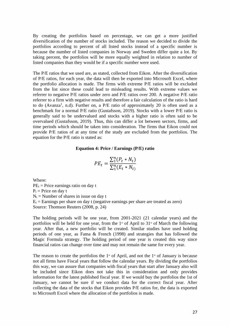
27

By creating the portfolios based on percentage, we can get a more justified

diversification of the number of stocks included. The reason we decided to divide the

portfolios according to percent of all listed stocks instead of a specific number is

because the number of listed companies in Norway and Sweden differ quite a lot. By

taking percent, the portfolios will be more equally weighted in relation to number of

listed companies than they would be if a specific number were used.

The P/E ratios that we used are, as stated, collected from Eikon. After the diversification

of P/E ratios, for each year, the data will then be exported into Microsoft Excel, where

the portfolio allocation is made. The firms with extreme P/E ratios will be excluded

from the list since these could lead to misleading results. With extreme values we

referrer to negative P/E ratios under zero and P/E ratios over 200. A negative P/E ratio

referrer to a firm with negative results and therefore a fair calculation of the ratio is hard

to do (Avanza1, n.d). Further on, a P/E ratio of approximately 20 is often used as a

benchmark for a normal P/E ratio (Gustafsson, 2019). Stocks with a lower P/E ratio is

generally said to be undervalued and stocks with a higher ratio is often said to be

overvalued (Gustafsson, 2019). Thus, this can differ a lot between sectors, firms, and

time periods which should be taken into consideration. The firms that Eikon could not

provide P/E ratios of at any time of the study are excluded from the portfolios. The

equation for the P/E ratio is stated as:

Equation 4: Price / Earnings (P/E) ratio

𝑃𝐸𝑡 =∑ (𝑃𝑡 ∗ 𝑁𝑡)𝑛

1

∑ (𝐸𝑡 ∗ 𝑁𝑡)𝑛1

Where:

PEt = Price earnings ratio on day t

Pt = Price on day t

Nt = Number of shares in issue on day t

Et = Earnings per share on day t (negative earnings per share are treated as zero) Source: Thomson Reuters (2008, p. 24)

The holding periods will be one year, from 2001-2021 (21 calendar years) and the

portfolios will be held for one year, from the 1st of April to 31st of March the following

year. After that, a new portfolio will be created. Similar studies have used holding

periods of one year, as Fama & French (1998) and strategies that has followed the

Magic Formula strategy. The holding period of one year is created this way since

financial ratios can change over time and may not remain the same for every year.

The reason to create the portfolios the 1st of April, and not the 1st of January is because

not all firms have Fiscal years that follow the calendar years. By dividing the portfolios

this way, we can assure that companies with fiscal years that start after January also will

be included since Eikon does not take this in consideration and only provides

information for the latest published fiscal year. If we would buy the portfolios the 1st of

January, we cannot be sure if we conduct data for the correct fiscal year. After

collecting the data of the stocks that Eikon provides P/E ratios for, the data is exported

to Microsoft Excel where the allocation of the portfolios is made.

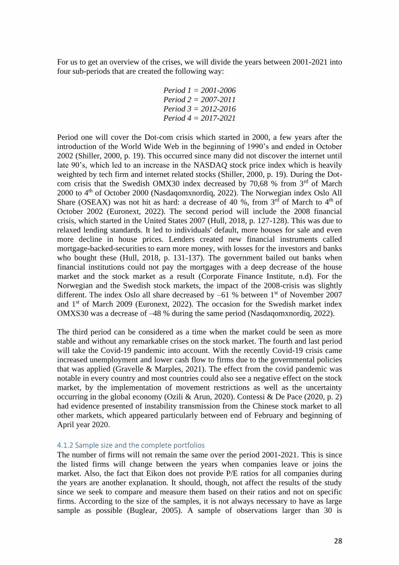
28

For us to get an overview of the crises, we will divide the years between 2001-2021 into

four sub-periods that are created the following way:

Period 1 = 2001-2006

Period 2 = 2007-2011

Period 3 = 2012-2016

Period 4 = 2017-2021

Period one will cover the Dot-com crisis which started in 2000, a few years after the

introduction of the World Wide Web in the beginning of 1990’s and ended in October

2002 (Shiller, 2000, p. 19). This occurred since many did not discover the internet until

late 90’s, which led to an increase in the NASDAQ stock price index which is heavily

weighted by tech firm and internet related stocks (Shiller, 2000, p. 19). During the Dot-

com crisis that the Swedish OMX30 index decreased by 70,68 % from 3rd of March

2000 to 4th of October 2000 (Nasdaqomxnordiq, 2022). The Norwegian index Oslo All

Share (OSEAX) was not hit as hard: a decrease of 40 %, from 3rd of March to 4th of

October 2002 (Euronext, 2022). The second period will include the 2008 financial

crisis, which started in the United States 2007 (Hull, 2018, p. 127-128). This was due to

relaxed lending standards. It led to individuals' default, more houses for sale and even

more decline in house prices. Lenders created new financial instruments called

mortgage-backed-securities to earn more money, with losses for the investors and banks

who bought these (Hull, 2018, p. 131-137). The government bailed out banks when

financial institutions could not pay the mortgages with a deep decrease of the house

market and the stock market as a result (Corporate Finance Institute, n.d). For the

Norwegian and the Swedish stock markets, the impact of the 2008-crisis was slightly

different. The index Oslo all share decreased by –61 % between 1st of November 2007

and 1st of March 2009 (Euronext, 2022). The occasion for the Swedish market index

OMXS30 was a decrease of –48 % during the same period (Nasdaqomxnordiq, 2022).

The third period can be considered as a time when the market could be seen as more

stable and without any remarkable crises on the stock market. The fourth and last period

will take the Covid-19 pandemic into account. With the recently Covid-19 crisis came

increased unemployment and lower cash flow to firms due to the governmental policies

that was applied (Gravelle & Marples, 2021). The effect from the covid pandemic was

notable in every country and most countries could also see a negative effect on the stock

market, by the implementation of movement restrictions as well as the uncertainty

occurring in the global economy (Ozili & Arun, 2020). Contessi & De Pace (2020, p. 2)

had evidence presented of instability transmission from the Chinese stock market to all

other markets, which appeared particularly between end of February and beginning of

April year 2020.

4.1.2 Sample size and the complete portfolios The number of firms will not remain the same over the period 2001-2021. This is since

the listed firms will change between the years when companies leave or joins the

market. Also, the fact that Eikon does not provide P/E ratios for all companies during

the years are another explanation. It should, though, not affect the results of the study

since we seek to compare and measure them based on their ratios and not on specific

firms. According to the size of the samples, it is not always necessary to have as large

sample as possible (Buglear, 2005). A sample of observations larger than 30 is

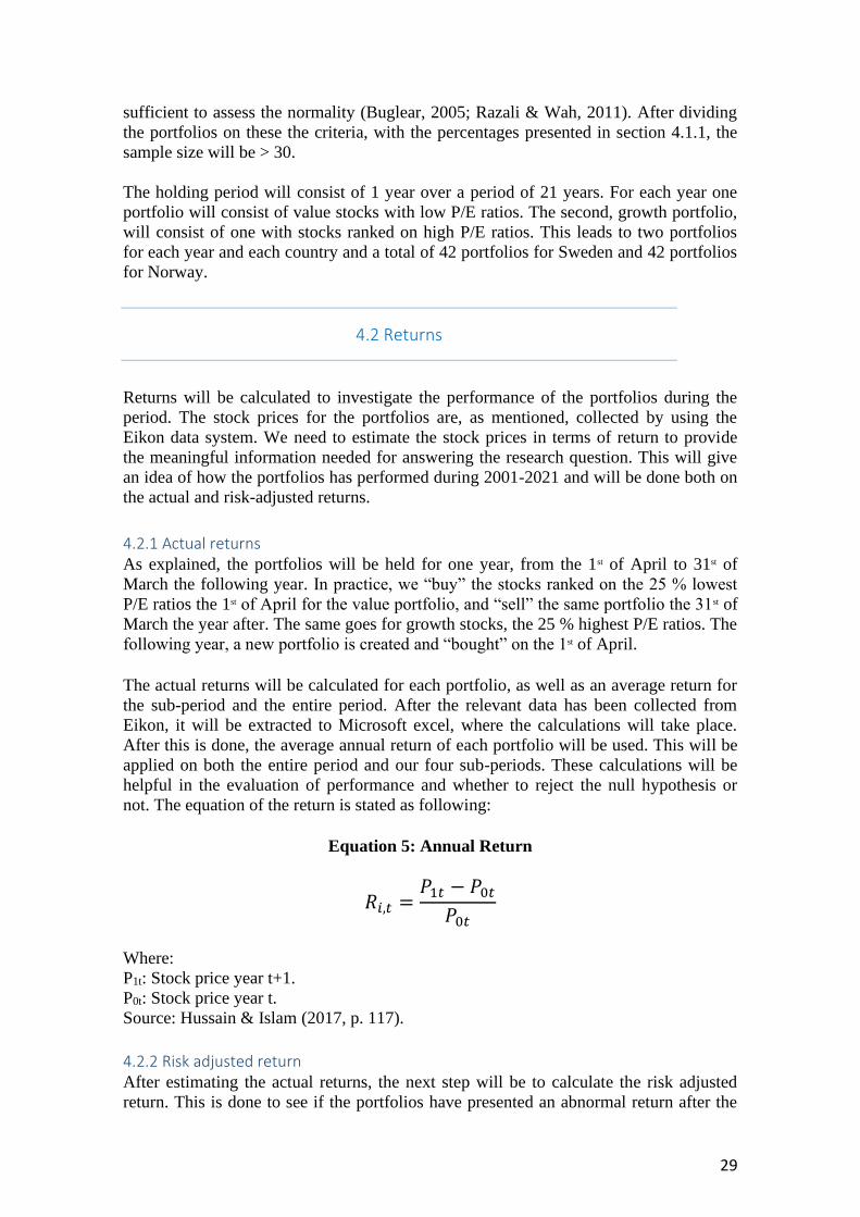
29

sufficient to assess the normality (Buglear, 2005; Razali & Wah, 2011). After dividing

the portfolios on these the criteria, with the percentages presented in section 4.1.1, the

sample size will be > 30.

The holding period will consist of 1 year over a period of 21 years. For each year one

portfolio will consist of value stocks with low P/E ratios. The second, growth portfolio,

will consist of one with stocks ranked on high P/E ratios. This leads to two portfolios

for each year and each country and a total of 42 portfolios for Sweden and 42 portfolios

for Norway.

4.2 Returns

Returns will be calculated to investigate the performance of the portfolios during the

period. The stock prices for the portfolios are, as mentioned, collected by using the

Eikon data system. We need to estimate the stock prices in terms of return to provide

the meaningful information needed for answering the research question. This will give

an idea of how the portfolios has performed during 2001-2021 and will be done both on

the actual and risk-adjusted returns.

4.2.1 Actual returns As explained, the portfolios will be held for one year, from the 1st of April to 31st of

March the following year. In practice, we “buy” the stocks ranked on the 25 % lowest

P/E ratios the 1st of April for the value portfolio, and “sell” the same portfolio the 31st of

March the year after. The same goes for growth stocks, the 25 % highest P/E ratios. The

following year, a new portfolio is created and “bought” on the 1st of April.

The actual returns will be calculated for each portfolio, as well as an average return for

the sub-period and the entire period. After the relevant data has been collected from

Eikon, it will be extracted to Microsoft excel, where the calculations will take place.

After this is done, the average annual return of each portfolio will be used. This will be

applied on both the entire period and our four sub-periods. These calculations will be

helpful in the evaluation of performance and whether to reject the null hypothesis or

not. The equation of the return is stated as following:

Equation 5: Annual Return

𝑅𝑖,𝑡 =𝑃1𝑡 − 𝑃0𝑡

𝑃0𝑡

Where: P1t: Stock price year t+1. P0t: Stock price year t.

Source: Hussain & Islam (2017, p. 117).

4.2.2 Risk adjusted return After estimating the actual returns, the next step will be to calculate the risk adjusted

return. This is done to see if the portfolios have presented an abnormal return after the

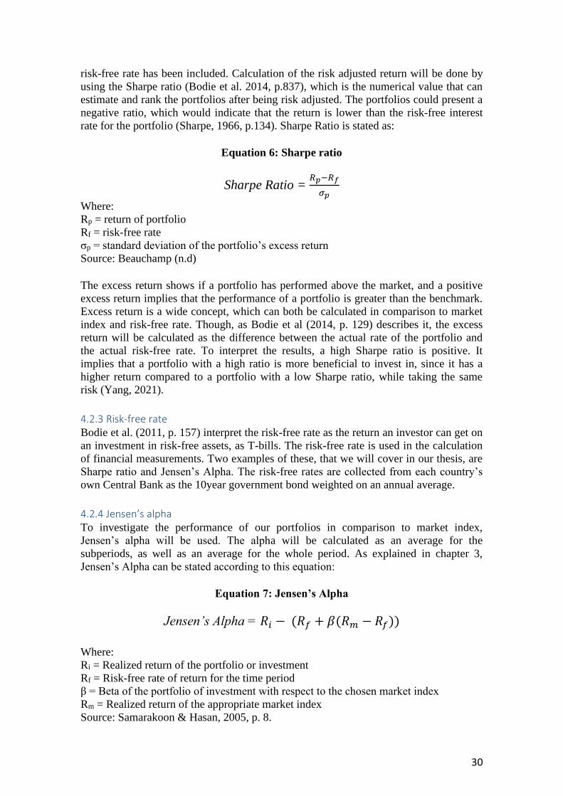
30

risk-free rate has been included. Calculation of the risk adjusted return will be done by

using the Sharpe ratio (Bodie et al. 2014, p.837), which is the numerical value that can

estimate and rank the portfolios after being risk adjusted. The portfolios could present a

negative ratio, which would indicate that the return is lower than the risk-free interest

rate for the portfolio (Sharpe, 1966, p.134). Sharpe Ratio is stated as:

Equation 6: Sharpe ratio

Sharpe Ratio = 𝑅𝑝−𝑅𝑓

𝜎𝑝

Where:

Rp = return of portfolio

Rf = risk-free rate

σp = standard deviation of the portfolio’s excess return Source: Beauchamp (n.d)

The excess return shows if a portfolio has performed above the market, and a positive

excess return implies that the performance of a portfolio is greater than the benchmark.

Excess return is a wide concept, which can both be calculated in comparison to market

index and risk-free rate. Though, as Bodie et al (2014, p. 129) describes it, the excess

return will be calculated as the difference between the actual rate of the portfolio and

the actual risk-free rate. To interpret the results, a high Sharpe ratio is positive. It

implies that a portfolio with a high ratio is more beneficial to invest in, since it has a

higher return compared to a portfolio with a low Sharpe ratio, while taking the same

risk (Yang, 2021).

4.2.3 Risk-free rate Bodie et al. (2011, p. 157) interpret the risk-free rate as the return an investor can get on

an investment in risk-free assets, as T-bills. The risk-free rate is used in the calculation

of financial measurements. Two examples of these, that we will cover in our thesis, are

Sharpe ratio and Jensen’s Alpha. The risk-free rates are collected from each country’s

own Central Bank as the 10year government bond weighted on an annual average.

4.2.4 Jensen’s alpha To investigate the performance of our portfolios in comparison to market index,

Jensen’s alpha will be used. The alpha will be calculated as an average for the

subperiods, as well as an average for the whole period. As explained in chapter 3,

Jensen’s Alpha can be stated according to this equation:

Equation 7: Jensen’s Alpha

Jensen’s Alpha = 𝑅𝑖 − (𝑅𝑓 + 𝛽(𝑅𝑚 − 𝑅𝑓))

Where:

Ri = Realized return of the portfolio or investment

Rf = Risk-free rate of return for the time period

β = Beta of the portfolio of investment with respect to the chosen market index

Rm = Realized return of the appropriate market index Source: Samarakoon & Hasan, 2005, p. 8.

31

Except for the realized return of the portfolios, market index returns and the risk-free

rate for the specific time periods, Beta also need to be calculated. A beta higher than 1

implies that the portfolio varies and moves more than the index, same time, a beta lower

than 1 implies that the portfolio fluctuates less than the index (Penman, 2010, p. 112).

The calculation of beta will be done In Microsoft Excel, using the following formula:

Equation 8: Beta

𝛽 = 𝐶𝑜𝑣 (𝑟𝑝,𝑟𝑚)

𝛿2(𝑟𝑚)

Where:

Cov = Covariance

δ2 = Variance

Source: Bodie et al (2011, p. 283)

When all the variables have been estimated, Jensen’s Alpha can be calculated. This

measurement is an important part of this study since it is the model that can prove if the

portfolios have performed an abnormal return compared to market index.

4.2.5 Market index returns As stated above, the market index returns are necessary to calculate Jensen’s Alpha. The

actual returns of the indices will also be used to examine how the portfolios has

performed; they will also be compared to market indexes. To get a fair comparison

between the countries, two similar market indexes will be used: Oslo All Share

(OSEAX) and Stockholm OMXSPI. OMXSPI, also called the all-share index, will be

used in Sweden, since it gives a summary of all the listed stocks on the Stockholm

exchange market (Avanza2, n.d). Oslo all share PR is an index that gives a summary of

all the listed stocks on Oslo Børs ASA. Since the return of the portfolios will be

compared to the market, the annual return of market index will be calculated. This is

done by using the Total return provided by Eikon.

4.3 Hypothesis

A statistical significance test of the findings should be made to know if the outcome of

the study can accept or reject the stated null hypotheses. As Bryman & Bell (2011, p.

353) explain, the test will determine how confident the researcher can be the findings

from the sample are applicable on the whole population. The statistical significance is

stated as levels of probability which represent the probability of rejecting the null

hypothesis when it should be approved (Bryman & Bell, 2011, p. 353). It can be

presented in different ways, yet the maximum level according to most of the researchers

that could be acceptable is 0.05 (Bryman & Bell, 2011, p. 353), which will be used in

this study when the hypotheses are tested. If one can reject a null hypothesis on a

32

significance level of 0.05 it implies that the results should not exist by chance and that

the risk of finding a relationship of a population when there isn‘t a relationship, should

not be bigger than 5 out of 100 (Bryman & Bell, 2011, p. 353).

When performing the test of a hypothesis, the researcher should have in mind that errors

might occur, which as Bryman & Bell (2011, p. 354) classify as type 1 and 2 errors.

Type 1 can be described as the error of an incorrectly rejected null hypothesis while

type 2 is the other way, to accept the null hypothesis when it should be rejected

(Bryman & Bell, 2011, p. 354), which will be taken in consideration.

The hypotheses will test the portfolios assorted depending on its P/E ratio. This will

help us decide if the portfolios consisting of growth stocks (high P/E ratios) will

outperform the value stocks (low P/E ratios) between 2001-2021 and in comparison, to

the market index. Further on, the sub-periods will investigate if any difference can be

seen between the countries and various financial times. Therefore, five hypotheses are

derived based on this and to provide a ground for answering the research questions. The

hypotheses that will be tested are stated as the following:

H01: A portfolio with high P/E stocks will not present a higher (actual) return than a

portfolio with low P/E stocks during the period 2001-2021 for Norway.

HA1: A portfolio with high P/E stocks will present a higher (actual) return than a

portfolio with low P/E stocks during the period 2001-2021 for Norway.

H02: A portfolio with high P/E stocks will not present a higher (actual) return than a

portfolio with low P/E stocks during the period 2001-2021 for Sweden.

HA2: A portfolio with high P/E stocks will present a higher (actual) return than a

portfolio with low P/E stocks during the period 2001-2021 for Sweden.

H03: A portfolio with high P/E stocks will not present a higher return than market index.

HA3: A portfolio with high P/E stocks will present a higher return than market index.

H04: A portfolio with low P/E stocks will not present a higher return than market index

return.

HA4: A portfolio with low P/E stocks will present a higher return than market index

return.

H05: A portfolio with high P/E stocks will not present a higher risk adjusted return than

a portfolio with low P/E stocks during the period 2001-2021.

HA5: A portfolio with high P/E stocks will present a higher risk adjusted return than a

portfolio with low P/E stocks during the period 2001-2021.

33

4.4 Normality

To interpret the hypothesis test in a correct manner, we need to test if our samples

follow a normal distribution. This will help us to determine which type of method to use

later in the study (Mishra et al., 2019, p. 69-70). To check whether the assumption of

normality holds or not, there are three common ways to test this according to Razali &

Wah (2011, p. 21). These are explained as graphical methods and a quantile-plot is the

most well-used method. Though, the authors explain that a graphical method is not

sufficient to show evidence that the assumption holds. Therefore, they state that

numerical methods and a formal normality test should be used. Shapiro wilks is said to

be the most common way to calculate the normality and a study of Razali & Wah

(2011) tests this numerical method against three other normality tests. The results shows

that Shapiro Wilks is the most powerful test to measure all types of distribution with

different kind of sample sizes (Razali & Wah, 2011). However, errors due to wrongfully

assumed data are common in the statistical procedure and one of these is the assumption

of a normally distributed sample (Curran-Everett & Benos, 2004, p. 189). This is

important to keep in mind when performing tests, since the reliability and accuracy of

reality might be affected by the wrong assumptions (Oztuna et al., 2006, p. 172).

4.5 Selection of significance test

After the normality testing of the samples are done, the hypothesis tests will be selected

to answer the hypothesises and to evaluate if the return of one portfolio is significantly

different from another. According to Corder & Foreman (2014) the significance tests

can be divided into two categories which are described as non-parametric and

parametric tests. One must know whether to use a parametric or non-parametric test,

which differ in terms on assumptions of the sample they investigate (Corder &

Foreman. 2014, p. 2-3). In an article made by Healthknowledge (2016) they presented

that a parametric test assume that the population follows a normal distribution while a

non-parametric test makes no assumptions on the sample and can therefore be used if

the sample does not follow a normal distribution. This provides more statistical power

to a parametric test (Healthknowledge, 2016).

However, there are more things to look at before making this decision and sample size

is one of them. Davidsson (1994) presents the concept of the central limit theorem

(CLT), which is well-known when performing statistical tests. According to the author

the CLT could assume that a population moves towards a normal distribution as the

sample size increase, even if tests and graphs suggest otherwise (Davidson, 1994,

p.364). It can be said that if the sample size >30, one could assume a normal

distribution (Kwak & Kim, 2017, p. 148), which will be taken in consideration.

4.5.1 Non-parametric tests The Mann-Whitney U test is a non-parametric statistic method that is used to measure

two independent samples, while the parametric equivalent to this test is the t-test

(Corder & Foreman. 2014, p. 69). The authors describe the idea behind this test as to

34

determine whether the sample values are randomly mixed in the rank ordering or

clustered at the opposite ends when combined. After the U statistic has been calculated,

one must examine it for significance which can be done by using critical values (Corder

& Foreman, 2014, p. 70-71). Also, the p-value method can be used to test the

significance of the result to find the probability (Shier, 2004, p. 2). Another non-

parametric test is the Wilcoxon signed rank test and can be defined as the alternative to

the paired sample t-test which is a parametric test (Verma &Abdel-Salam, 2019, p. 168-

172). As the authors explain, this method aims to test the significance between

dependent variables based on its mean. The sample can come from the same population

or populations with comparable characteristics. Though, some violations of the

assumption that can cause problems for this method is if the samples view tendency of

being independent, if that is the case, the Mann Whitney U-test is more appropriate

(Verma &Abdel-Salam, 2019, p. 168-172).

4.5.2 Parametric tests According to Verma & Abdel-Salam (2019, p. 92) the independent sample t-test is one

of the most common and widely used parametric tests, where the goal is to compare two

separate populations or groups based on their differences. Data used for this test needs

to be free from outliners and the dependent variable must be continuous. Further on, the

authors explain that its data must contain data that is collected randomly and follow a

normal distribution (Verma &Abdel-Salam, 2019, p. 92).

Kent State University (2022) state that the paired sample t-test is a parametric test used

to evaluate the same individual, units, or objects in comparison to different time

periods. This test determines if the mean difference between paired observations is

substantially different from zero, based on statistical evidence. Some of the assumptions

that are required to be fulfilled to use this test is, normal distribution of the difference

between values, the subjects in the two groups are the same, no outliers and the data is

collected randomly (Kent State University, 2022).

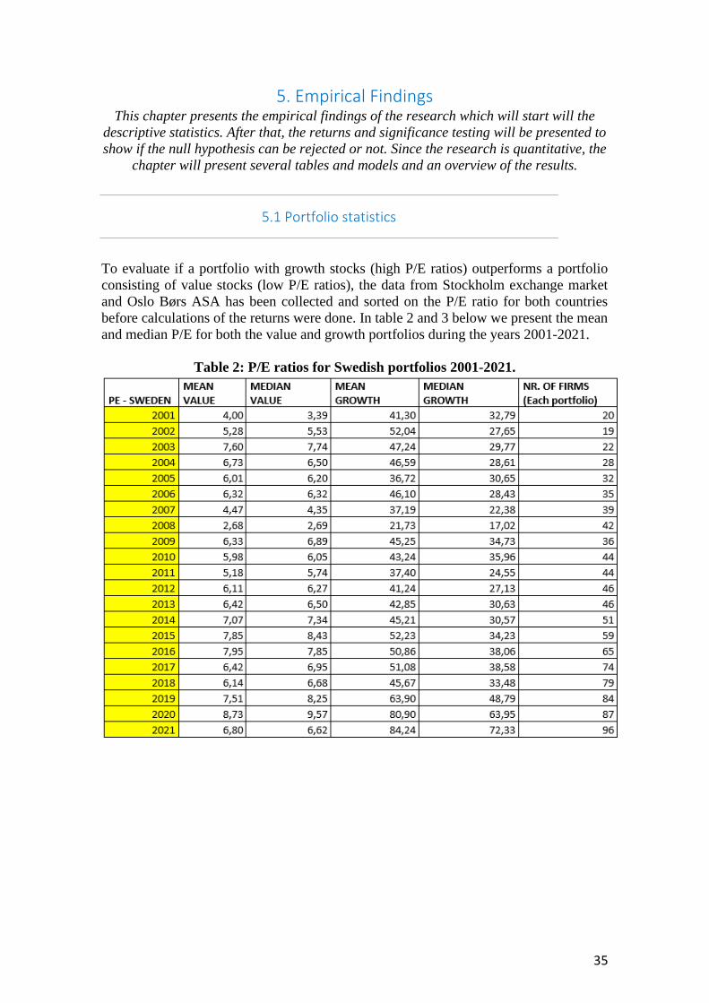
35

5. Empirical Findings This chapter presents the empirical findings of the research which will start will the

descriptive statistics. After that, the returns and significance testing will be presented to

show if the null hypothesis can be rejected or not. Since the research is quantitative, the

chapter will present several tables and models and an overview of the results.

5.1 Portfolio statistics

To evaluate if a portfolio with growth stocks (high P/E ratios) outperforms a portfolio

consisting of value stocks (low P/E ratios), the data from Stockholm exchange market

and Oslo Børs ASA has been collected and sorted on the P/E ratio for both countries

before calculations of the returns were done. In table 2 and 3 below we present the mean

and median P/E for both the value and growth portfolios during the years 2001-2021.

Table 2: P/E ratios for Swedish portfolios 2001-2021.

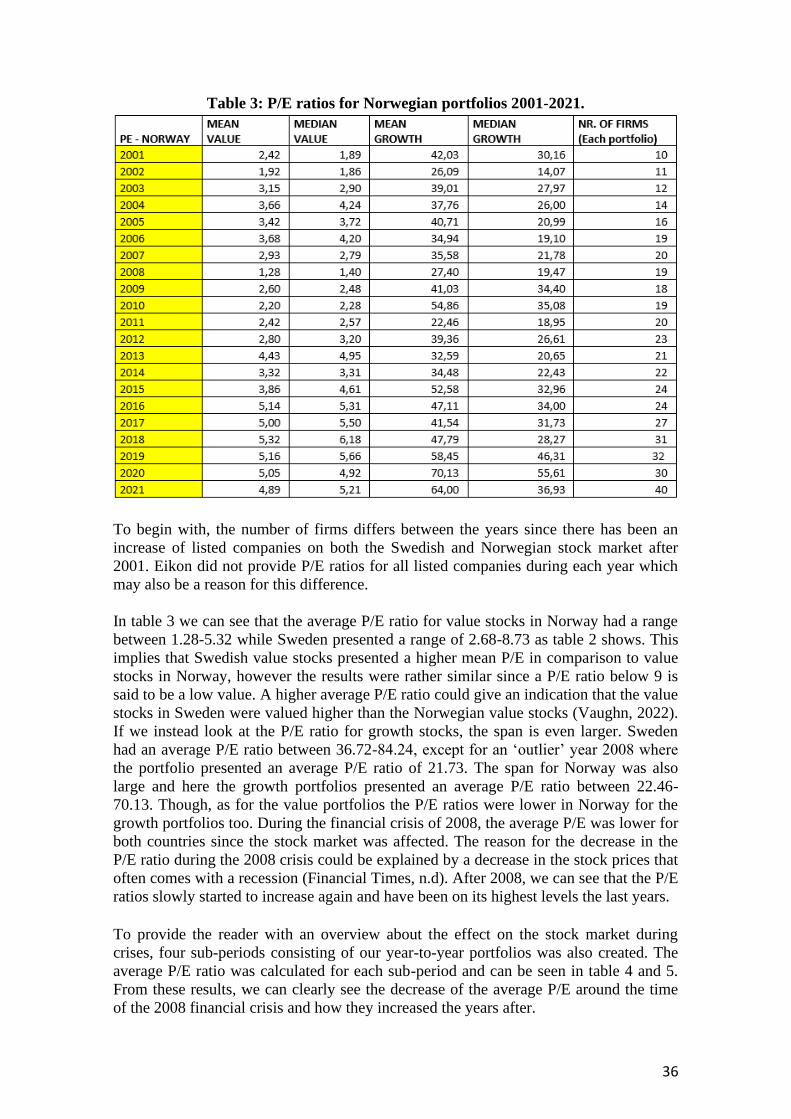
36

Table 3: P/E ratios for Norwegian portfolios 2001-2021.

To begin with, the number of firms differs between the years since there has been an

increase of listed companies on both the Swedish and Norwegian stock market after

2001. Eikon did not provide P/E ratios for all listed companies during each year which

may also be a reason for this difference.

In table 3 we can see that the average P/E ratio for value stocks in Norway had a range

between 1.28-5.32 while Sweden presented a range of 2.68-8.73 as table 2 shows. This

implies that Swedish value stocks presented a higher mean P/E in comparison to value

stocks in Norway, however the results were rather similar since a P/E ratio below 9 is

said to be a low value. A higher average P/E ratio could give an indication that the value

stocks in Sweden were valued higher than the Norwegian value stocks (Vaughn, 2022).

If we instead look at the P/E ratio for growth stocks, the span is even larger. Sweden

had an average P/E ratio between 36.72-84.24, except for an ‘outlier’ year 2008 where

the portfolio presented an average P/E ratio of 21.73. The span for Norway was also

large and here the growth portfolios presented an average P/E ratio between 22.46-

70.13. Though, as for the value portfolios the P/E ratios were lower in Norway for the

growth portfolios too. During the financial crisis of 2008, the average P/E was lower for

both countries since the stock market was affected. The reason for the decrease in the

P/E ratio during the 2008 crisis could be explained by a decrease in the stock prices that

often comes with a recession (Financial Times, n.d). After 2008, we can see that the P/E

ratios slowly started to increase again and have been on its highest levels the last years.

To provide the reader with an overview about the effect on the stock market during

crises, four sub-periods consisting of our year-to-year portfolios was also created. The

average P/E ratio was calculated for each sub-period and can be seen in table 4 and 5.

From these results, we can clearly see the decrease of the average P/E around the time

of the 2008 financial crisis and how they increased the years after.

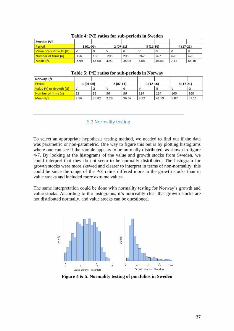
37

Table 4: P/E ratios for sub-periods in Sweden

Table 5: P/E ratios for sub-periods in Norway

5.2 Normality testing

To select an appropriate hypothesis testing method, we needed to find out if the data

was parametric or non-parametric. One way to figure this out is by plotting histograms

where one can see if the sample appears to be normally distributed, as shown in figure

4-7. By looking at the histograms of the value and growth stocks from Sweden, we

could interpret that they do not seem to be normally distributed. The histogram for

growth stocks were more skewed and clearer to interpret in terms of non-normality, this

could be since the range of the P/E ratios differed more in the growth stocks than in

value stocks and included more extreme values.

The same interpretation could be done with normality testing for Norway’s growth and

value stocks. According to the histograms, it’s noticeably clear that growth stocks are

not distributed normally, and value stocks can be questioned.

Figure 4 & 5. Normality testing of portfolios in Sweden

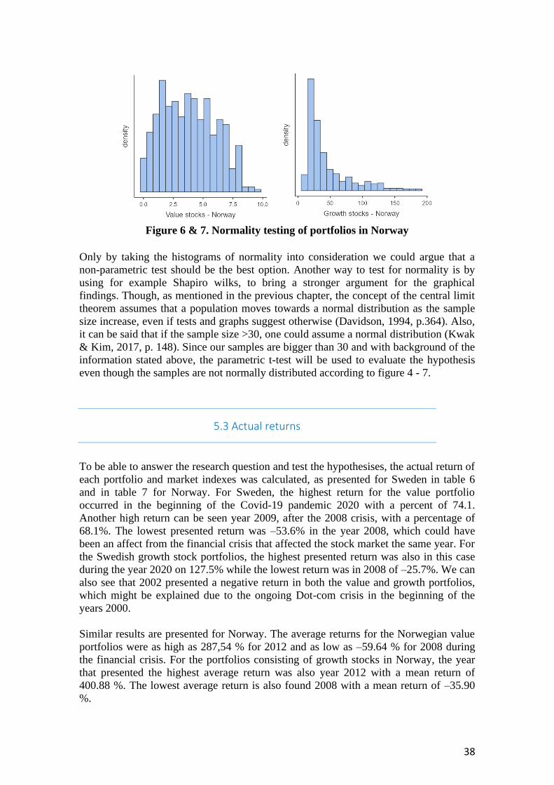
38

Figure 6 & 7. Normality testing of portfolios in Norway

Only by taking the histograms of normality into consideration we could argue that a

non-parametric test should be the best option. Another way to test for normality is by

using for example Shapiro wilks, to bring a stronger argument for the graphical

findings. Though, as mentioned in the previous chapter, the concept of the central limit

theorem assumes that a population moves towards a normal distribution as the sample

size increase, even if tests and graphs suggest otherwise (Davidson, 1994, p.364). Also,

it can be said that if the sample size >30, one could assume a normal distribution (Kwak

& Kim, 2017, p. 148). Since our samples are bigger than 30 and with background of the

information stated above, the parametric t-test will be used to evaluate the hypothesis

even though the samples are not normally distributed according to figure 4 - 7.

5.3 Actual returns

To be able to answer the research question and test the hypothesises, the actual return of

each portfolio and market indexes was calculated, as presented for Sweden in table 6

and in table 7 for Norway. For Sweden, the highest return for the value portfolio

occurred in the beginning of the Covid-19 pandemic 2020 with a percent of 74.1.

Another high return can be seen year 2009, after the 2008 crisis, with a percentage of

68.1%. The lowest presented return was –53.6% in the year 2008, which could have

been an affect from the financial crisis that affected the stock market the same year. For

the Swedish growth stock portfolios, the highest presented return was also in this case

during the year 2020 on 127.5% while the lowest return was in 2008 of –25.7%. We can

also see that 2002 presented a negative return in both the value and growth portfolios,

which might be explained due to the ongoing Dot-com crisis in the beginning of the

years 2000.

Similar results are presented for Norway. The average returns for the Norwegian value

portfolios were as high as 287,54 % for 2012 and as low as –59.64 % for 2008 during

the financial crisis. For the portfolios consisting of growth stocks in Norway, the year

that presented the highest average return was also year 2012 with a mean return of

400.88 %. The lowest average return is also found 2008 with a mean return of –35.90

%.

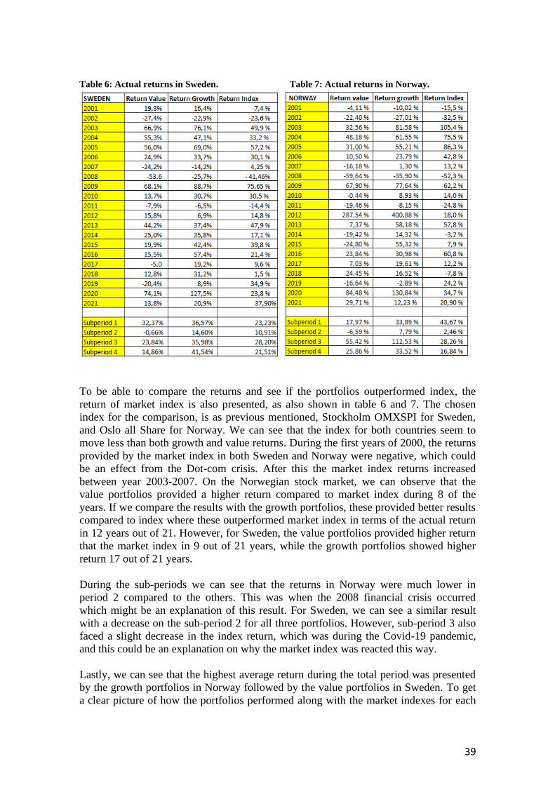
39

Table 6: Actual returns in Sweden. Table 7: Actual returns in Norway.

To be able to compare the returns and see if the portfolios outperformed index, the

return of market index is also presented, as also shown in table 6 and 7. The chosen

index for the comparison, is as previous mentioned, Stockholm OMXSPI for Sweden,

and Oslo all Share for Norway. We can see that the index for both countries seem to

move less than both growth and value returns. During the first years of 2000, the returns

provided by the market index in both Sweden and Norway were negative, which could

be an effect from the Dot-com crisis. After this the market index returns increased

between year 2003-2007. On the Norwegian stock market, we can observe that the

value portfolios provided a higher return compared to market index during 8 of the

years. If we compare the results with the growth portfolios, these provided better results

compared to index where these outperformed market index in terms of the actual return

in 12 years out of 21. However, for Sweden, the value portfolios provided higher return

that the market index in 9 out of 21 years, while the growth portfolios showed higher

return 17 out of 21 years.

During the sub-periods we can see that the returns in Norway were much lower in

period 2 compared to the others. This was when the 2008 financial crisis occurred

which might be an explanation of this result. For Sweden, we can see a similar result

with a decrease on the sub-period 2 for all three portfolios. However, sub-period 3 also

faced a slight decrease in the index return, which was during the Covid-19 pandemic,

and this could be an explanation on why the market index was reacted this way.

Lastly, we can see that the highest average return during the total period was presented

by the growth portfolios in Norway followed by the value portfolios in Sweden. To get

a clear picture of how the portfolios performed along with the market indexes for each

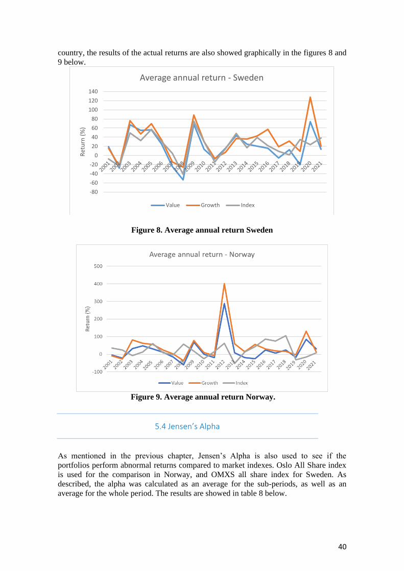
40

country, the results of the actual returns are also showed graphically in the figures 8 and

9 below.

Figure 8. Average annual return Sweden

Figure 9. Average annual return Norway.

5.4 Jensen’s Alpha

As mentioned in the previous chapter, Jensen’s Alpha is also used to see if the

portfolios perform abnormal returns compared to market indexes. Oslo All Share index

is used for the comparison in Norway, and OMXS all share index for Sweden. As

described, the alpha was calculated as an average for the sub-periods, as well as an

average for the whole period. The results are showed in table 8 below.

-80

-60

-40

-20

0

20

40

60

80

100

120

140

Ret

urn

(%

)Average annual return - Sweden

Value Growth Index

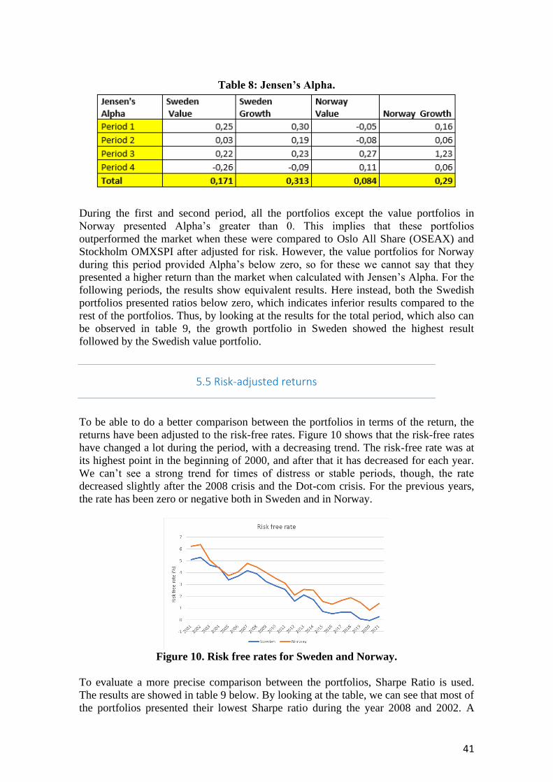
41

Table 8: Jensen’s Alpha.

During the first and second period, all the portfolios except the value portfolios in

Norway presented Alpha’s greater than 0. This implies that these portfolios

outperformed the market when these were compared to Oslo All Share (OSEAX) and

Stockholm OMXSPI after adjusted for risk. However, the value portfolios for Norway

during this period provided Alpha’s below zero, so for these we cannot say that they

presented a higher return than the market when calculated with Jensen’s Alpha. For the

following periods, the results show equivalent results. Here instead, both the Swedish

portfolios presented ratios below zero, which indicates inferior results compared to the

rest of the portfolios. Thus, by looking at the results for the total period, which also can

be observed in table 9, the growth portfolio in Sweden showed the highest result

followed by the Swedish value portfolio.

5.5 Risk-adjusted returns

To be able to do a better comparison between the portfolios in terms of the return, the

returns have been adjusted to the risk-free rates. Figure 10 shows that the risk-free rates

have changed a lot during the period, with a decreasing trend. The risk-free rate was at

its highest point in the beginning of 2000, and after that it has decreased for each year.

We can’t see a strong trend for times of distress or stable periods, though, the rate

decreased slightly after the 2008 crisis and the Dot-com crisis. For the previous years,

the rate has been zero or negative both in Sweden and in Norway.

Figure 10. Risk free rates for Sweden and Norway.

To evaluate a more precise comparison between the portfolios, Sharpe Ratio is used.

The results are showed in table 9 below. By looking at the table, we can see that most of

the portfolios presented their lowest Sharpe ratio during the year 2008 and 2002. A

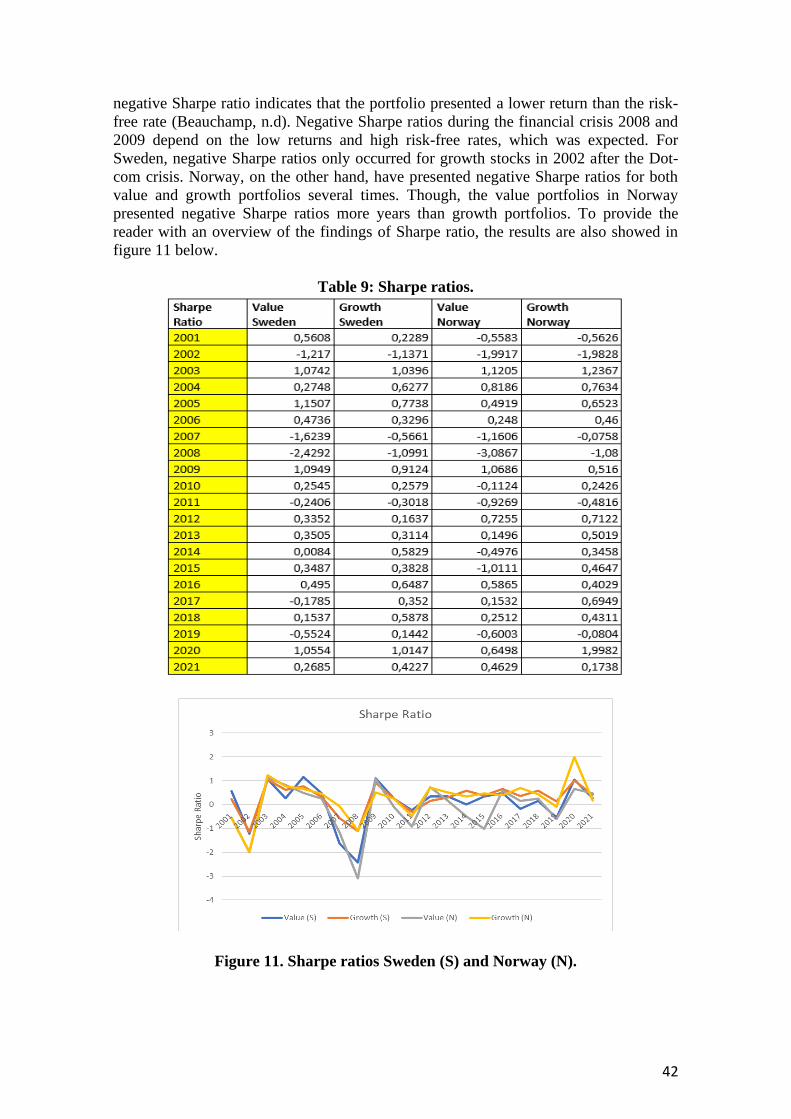
42

negative Sharpe ratio indicates that the portfolio presented a lower return than the risk-

free rate (Beauchamp, n.d). Negative Sharpe ratios during the financial crisis 2008 and

2009 depend on the low returns and high risk-free rates, which was expected. For

Sweden, negative Sharpe ratios only occurred for growth stocks in 2002 after the Dot-

com crisis. Norway, on the other hand, have presented negative Sharpe ratios for both

value and growth portfolios several times. Though, the value portfolios in Norway

presented negative Sharpe ratios more years than growth portfolios. To provide the

reader with an overview of the findings of Sharpe ratio, the results are also showed in

figure 11 below.

Table 9: Sharpe ratios.

Figure 11. Sharpe ratios Sweden (S) and Norway (N).

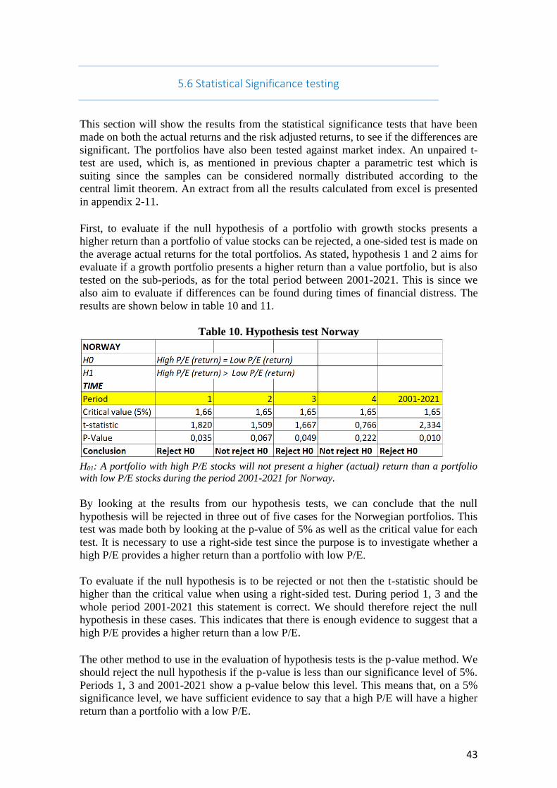
43

5.6 Statistical Significance testing

This section will show the results from the statistical significance tests that have been

made on both the actual returns and the risk adjusted returns, to see if the differences are

significant. The portfolios have also been tested against market index. An unpaired t-

test are used, which is, as mentioned in previous chapter a parametric test which is

suiting since the samples can be considered normally distributed according to the

central limit theorem. An extract from all the results calculated from excel is presented

in appendix 2-11.

First, to evaluate if the null hypothesis of a portfolio with growth stocks presents a

higher return than a portfolio of value stocks can be rejected, a one-sided test is made on

the average actual returns for the total portfolios. As stated, hypothesis 1 and 2 aims for

evaluate if a growth portfolio presents a higher return than a value portfolio, but is also

tested on the sub-periods, as for the total period between 2001-2021. This is since we

also aim to evaluate if differences can be found during times of financial distress. The

results are shown below in table 10 and 11.

Table 10. Hypothesis test Norway

H01: A portfolio with high P/E stocks will not present a higher (actual) return than a portfolio

with low P/E stocks during the period 2001-2021 for Norway.

By looking at the results from our hypothesis tests, we can conclude that the null

hypothesis will be rejected in three out of five cases for the Norwegian portfolios. This

test was made both by looking at the p-value of 5% as well as the critical value for each

test. It is necessary to use a right-side test since the purpose is to investigate whether a

high P/E provides a higher return than a portfolio with low P/E.

To evaluate if the null hypothesis is to be rejected or not then the t-statistic should be

higher than the critical value when using a right-sided test. During period 1, 3 and the

whole period 2001-2021 this statement is correct. We should therefore reject the null

hypothesis in these cases. This indicates that there is enough evidence to suggest that a

high P/E provides a higher return than a low P/E.

The other method to use in the evaluation of hypothesis tests is the p-value method. We

should reject the null hypothesis if the p-value is less than our significance level of 5%.

Periods 1, 3 and 2001-2021 show a p-value below this level. This means that, on a 5%

significance level, we have sufficient evidence to say that a high P/E will have a higher

return than a portfolio with a low P/E.

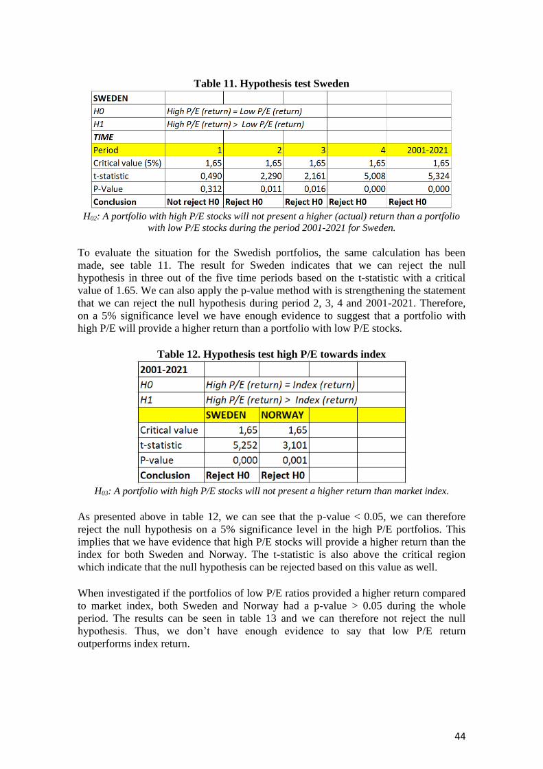
44

Table 11. Hypothesis test Sweden

H02: A portfolio with high P/E stocks will not present a higher (actual) return than a portfolio

with low P/E stocks during the period 2001-2021 for Sweden.

To evaluate the situation for the Swedish portfolios, the same calculation has been

made, see table 11. The result for Sweden indicates that we can reject the null

hypothesis in three out of the five time periods based on the t-statistic with a critical

value of 1.65. We can also apply the p-value method with is strengthening the statement

that we can reject the null hypothesis during period 2, 3, 4 and 2001-2021. Therefore,

on a 5% significance level we have enough evidence to suggest that a portfolio with

high P/E will provide a higher return than a portfolio with low P/E stocks.

Table 12. Hypothesis test high P/E towards index

H03: A portfolio with high P/E stocks will not present a higher return than market index.

As presented above in table 12, we can see that the p-value < 0.05, we can therefore

reject the null hypothesis on a 5% significance level in the high P/E portfolios. This

implies that we have evidence that high P/E stocks will provide a higher return than the

index for both Sweden and Norway. The t-statistic is also above the critical region

which indicate that the null hypothesis can be rejected based on this value as well.

When investigated if the portfolios of low P/E ratios provided a higher return compared

to market index, both Sweden and Norway had a p-value > 0.05 during the whole

period. The results can be seen in table 13 and we can therefore not reject the null

hypothesis. Thus, we don’t have enough evidence to say that low P/E return

outperforms index return.

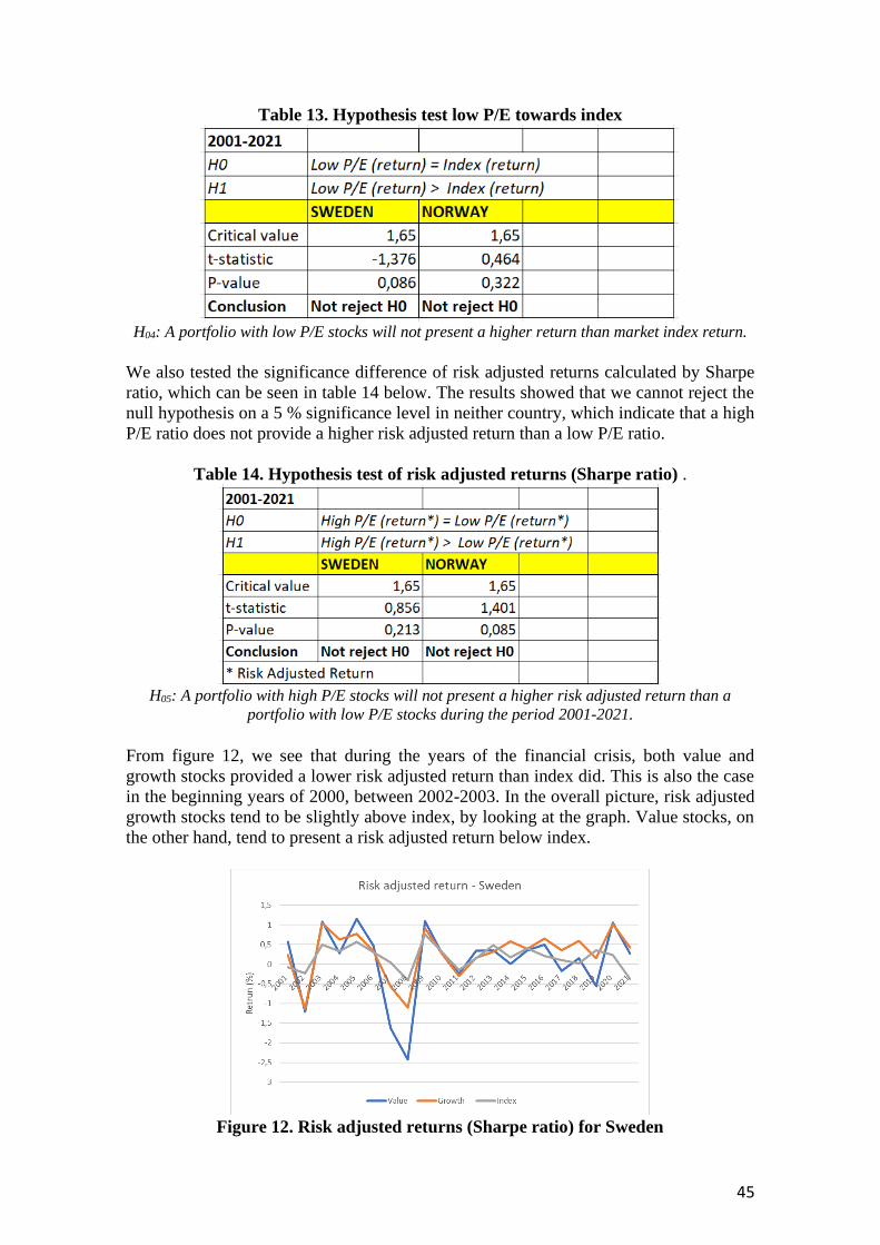
45

Table 13. Hypothesis test low P/E towards index

H04: A portfolio with low P/E stocks will not present a higher return than market index return.

We also tested the significance difference of risk adjusted returns calculated by Sharpe

ratio, which can be seen in table 14 below. The results showed that we cannot reject the

null hypothesis on a 5 % significance level in neither country, which indicate that a high

P/E ratio does not provide a higher risk adjusted return than a low P/E ratio.

Table 14. Hypothesis test of risk adjusted returns (Sharpe ratio) .

H05: A portfolio with high P/E stocks will not present a higher risk adjusted return than a

portfolio with low P/E stocks during the period 2001-2021.

From figure 12, we see that during the years of the financial crisis, both value and

growth stocks provided a lower risk adjusted return than index did. This is also the case

in the beginning years of 2000, between 2002-2003. In the overall picture, risk adjusted

growth stocks tend to be slightly above index, by looking at the graph. Value stocks, on

the other hand, tend to present a risk adjusted return below index.

Figure 12. Risk adjusted returns (Sharpe ratio) for Sweden

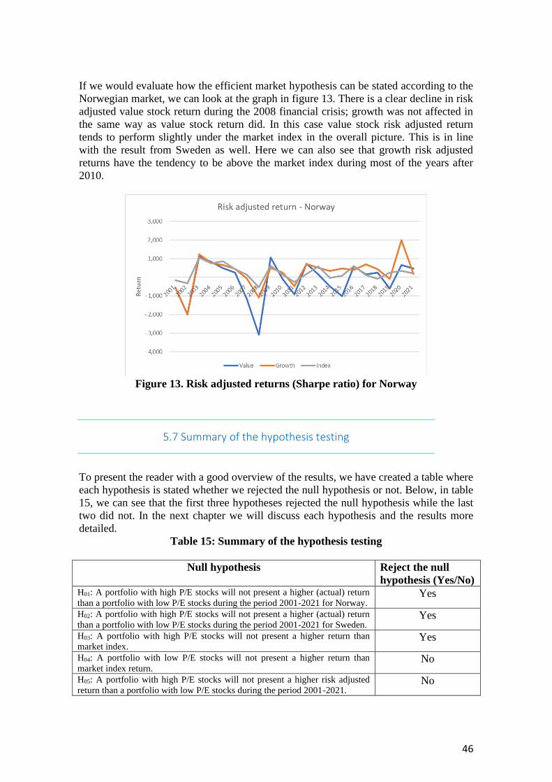
46

If we would evaluate how the efficient market hypothesis can be stated according to the

Norwegian market, we can look at the graph in figure 13. There is a clear decline in risk

adjusted value stock return during the 2008 financial crisis; growth was not affected in

the same way as value stock return did. In this case value stock risk adjusted return

tends to perform slightly under the market index in the overall picture. This is in line

with the result from Sweden as well. Here we can also see that growth risk adjusted

returns have the tendency to be above the market index during most of the years after

2010.

Figure 13. Risk adjusted returns (Sharpe ratio) for Norway

5.7 Summary of the hypothesis testing

To present the reader with a good overview of the results, we have created a table where

each hypothesis is stated whether we rejected the null hypothesis or not. Below, in table

15, we can see that the first three hypotheses rejected the null hypothesis while the last

two did not. In the next chapter we will discuss each hypothesis and the results more

detailed.

Table 15: Summary of the hypothesis testing

Null hypothesis Reject the null

hypothesis (Yes/No) H01: A portfolio with high P/E stocks will not present a higher (actual) return

than a portfolio with low P/E stocks during the period 2001-2021 for Norway. Yes

H02: A portfolio with high P/E stocks will not present a higher (actual) return

than a portfolio with low P/E stocks during the period 2001-2021 for Sweden. Yes

H03: A portfolio with high P/E stocks will not present a higher return than

market index. Yes

H04: A portfolio with low P/E stocks will not present a higher return than

market index return. No

H05: A portfolio with high P/E stocks will not present a higher risk adjusted

return than a portfolio with low P/E stocks during the period 2001-2021. No

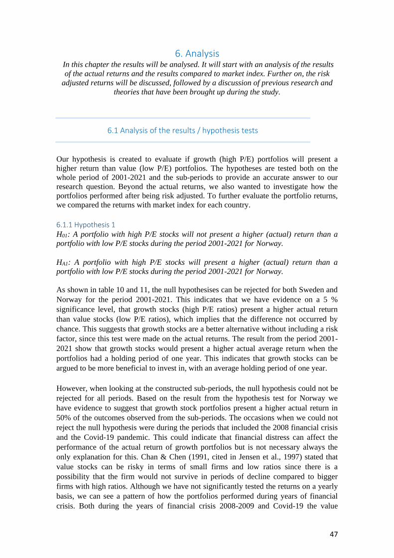
47

6. Analysis

In this chapter the results will be analysed. It will start with an analysis of the results

of the actual returns and the results compared to market index. Further on, the risk

adjusted returns will be discussed, followed by a discussion of previous research and

theories that have been brought up during the study.

6.1 Analysis of the results / hypothesis tests

Our hypothesis is created to evaluate if growth (high P/E) portfolios will present a

higher return than value (low P/E) portfolios. The hypotheses are tested both on the

whole period of 2001-2021 and the sub-periods to provide an accurate answer to our

research question. Beyond the actual returns, we also wanted to investigate how the

portfolios performed after being risk adjusted. To further evaluate the portfolio returns,

we compared the returns with market index for each country.

6.1.1 Hypothesis 1 H01: A portfolio with high P/E stocks will not present a higher (actual) return than a

portfolio with low P/E stocks during the period 2001-2021 for Norway.

HA1: A portfolio with high P/E stocks will present a higher (actual) return than a

portfolio with low P/E stocks during the period 2001-2021 for Norway.

As shown in table 10 and 11, the null hypothesises can be rejected for both Sweden and

Norway for the period 2001-2021. This indicates that we have evidence on a 5 %

significance level, that growth stocks (high P/E ratios) present a higher actual return

than value stocks (low P/E ratios), which implies that the difference not occurred by

chance. This suggests that growth stocks are a better alternative without including a risk

factor, since this test were made on the actual returns. The result from the period 2001-

2021 show that growth stocks would present a higher actual average return when the

portfolios had a holding period of one year. This indicates that growth stocks can be

argued to be more beneficial to invest in, with an average holding period of one year.

However, when looking at the constructed sub-periods, the null hypothesis could not be

rejected for all periods. Based on the result from the hypothesis test for Norway we

have evidence to suggest that growth stock portfolios present a higher actual return in

50% of the outcomes observed from the sub-periods. The occasions when we could not

reject the null hypothesis were during the periods that included the 2008 financial crisis

and the Covid-19 pandemic. This could indicate that financial distress can affect the

performance of the actual return of growth portfolios but is not necessary always the

only explanation for this. Chan & Chen (1991, cited in Jensen et al., 1997) stated that

value stocks can be risky in terms of small firms and low ratios since there is a

possibility that the firm would not survive in periods of decline compared to bigger

firms with high ratios. Although we have not significantly tested the returns on a yearly

basis, we can see a pattern of how the portfolios performed during years of financial

crisis. Both during the years of financial crisis 2008-2009 and Covid-19 the value

48

portfolios presented a lower return than the growth portfolios, which also here indicated

that holding a portfolio of growth stocks during times of financial distress can be a

better investment than investing in value stocks. But as stated, we do not have evidence

to conclude that on a 5 % significance level, we cannot be sure that the findings of the

samples are caused by chance. So even if the null hypotheses could not be rejected, we

can state that these observations talk for the same as Chan & Chen (1991) findings.

During the first period including the Dot-com crisis in the beginning of 2000’s, the null

hypothesis could though be rejected, which implies that we have evidence that the

portfolios of growth stocks presented a higher return compared to the value portfolios.

Although, looking at table 11, the pattern could not be observed graphically during the

greatest decline during Dot-com crisis (2000-2002) in Norway. Here we can observe

that the portfolios presented almost as high returns, which can imply that the evidence

of a higher return of the growth portfolios may not have been a cause of the crisis.

Though, we can see that the growth portfolios seemed to recover more rapidly than the

value portfolios after the Dot-com crisis.

6.1.2 Hypothesis 2

H02: A portfolio with high P/E stocks will not present a higher (actual) return than a

portfolio with low P/E stocks during the period 2001-2021 for Sweden.

HA2: A portfolio with high P/E stocks will present a higher (actual) return than a

portfolio with low P/E stocks during the period 2001-2021 for Sweden.

As stated, the null hypothesis could also be rejected when testing the Swedish

portfolios. Though, when tests were made on the four sub-periods, we have evidence to

suggest that the null hypothesis should be rejected in 75% of the cases. The explanation

of this could be that even during times of financial distress, a portfolio consisting of

growth stocks would be a better investment strategy for investors. If we were to

evaluate the result from the period 2001-2021, this provided similar outcomes as the

sub-periods. The implication of this could suggest that growth stocks would present a

higher actual average return when the portfolios had a holding period of one year. From

figure 10, when looking at the actual returns graphically, we can clearly see that the

portfolios consisting of growth stocks in Sweden presented a higher actual return than

the portfolio of value stocks. This were the occasion both during the Dot-com crisis that

reached to 2002, during the 2008 financial crisis and even during the Covid-19 crisis in

the beginning of 2020, which implies that the growth portfolios even are a better choice

than value portfolios during financial crisis.

We can thus say that we have evidence on a 5 % significance to suggest that the actual

return of growth portfolios (high P/E ratios) are higher compared to a portfolio of value

stocks (low P/E ratios). However, since the null hypothesis could be rejected more times

for Sweden compared to Norway when evaluating the four sub-periods, we can look at

that from a perspective of the financial crisis. This could imply that it could be an even

better strategy to stick with growth portfolios even during a time of financial distress on

the Swedish stock market compared to the Norwegian market.

49

Also, the repo rate in Sweden and Norway were significantly higher during 2000-2010

compared to the last decade. In times of low rates, growth stocks generally present

higher stock prices and returns than in times of high rates. Looking at figure 10, we can

graphically see that the difference between the return of the growth and value portfolios

in Sweden is bigger after 2013 than the difference was before that, which can be a cause

of the lower rates. Also, for Sweden, the only time the null hypothesis could not be

rejected were during the first period (2001-2006), when the rate was as highest which

could have affected that the growth portfolios did not provide as high returns compared

to the rest of the periods.

6.1.3 Hypothesis 3

H03: A portfolio with high P/E stocks will not present a higher return than market index.

HA3: A portfolio with high P/E stocks will present a higher return than market index.

To strengthen the founded evidence of a higher return of growth stocks compared to

value stocks, we included the market index as well to test the growth portfolios against

market index. From table 12, we can observe that both Sweden and Norway presented a

low p-value, and the null hypothesis could therefore be rejected. This means that growth

stocks (high P/E ratio) presented a higher actual return than the market index return and

indicates that holding a portfolio of growth stocks can be a better investment strategy

than follow the market index. Though, as mentioned, have we only tested the portfolios

against Oslo All Share (OSEAX) and Stockholm OMXSPI. Other indices might, of

course, have provided different returns.

Concerning Jensen’s Alpha, an alpha greater than 0 shows that the portfolio has

presented a higher return compared to market index (Jensen, 1968). For the first and

second period, all the portfolios presented alpha’s below 0, except the growth portfolio

for Norway. This indicates that the portfolios did not perform an abnormal return

compared to market index. For the 4th sub-period, all portfolios presented an alpha

greater than 0 and can therefore be said that all the portfolios showed an abnormal

return. For the whole period, the growth portfolio in Norway showed the highest result,

followed by the growth portfolio in Sweden. However, all portfolios presented an Alpha

greater than 0 which implied that both value and growth portfolios presented an

abnormal return compared to market.

6.1.4 Hypothesis 4 H04: A portfolio with low P/E stocks will not present a higher return than market index

return.

HA4: A portfolio with low P/E stocks will present a higher return than market index

return.

We also wanted to evaluate how the value portfolios performed in comparison to index,

which can be seen under table 13. Both countries failed to reject the null hypotheses

,based on the actual returns, which indicate that following index would be more

beneficial for investors than building portfolios with value stocks. This statement is

supported by presenting a higher p-value than 5% and a critical value below the critical

50

level. Though, as mentioned, the portfolios was only tested against Oslo All Share

(OSEAX) and Stockholm OMXSPI and might therefore provide another result for other

indices.

By looking at table 9, we can see that our value stock portfolios in Sweden presented an

alpha above 0 in the first three periods while Norway had a positive alpha the last two

periods. A positive alpha, above 0, can in this case indicate that the portfolios did

perform an abnormal return compared to market index. The total average for value

portfolios, both provided a positive alpha.

6.1.5 Hypothesis 5 H05: A portfolio with high P/E stocks will not present a higher risk adjusted return than

a portfolio with low P/E stocks during the period 2001-2021.

HA5: A portfolio with high P/E stocks will present a higher risk adjusted return than a

portfolio with low P/E stocks during the period 2001-2021.

A test for the risk-adjusted returns was similarly executed using the Sharpe ratio, these

can be seen under table 14. By taking both the p-value and t-statistic into consideration,

we cannot statistically determine that a portfolio of growth stocks provides a higher

return than a portfolio of value stocks during the period 2001-2021, as we could for the

actual returns. Norway presented similar results as Sweden did, which implies that after

adjusting the stock return in terms of risk we do not have enough evidence to say that a

portfolio with growth stocks would provide a higher return than a portfolio with value

stocks. Hence, we cannot say that the differences of the portfolios in Sweden and

Norway are affected by chance.

Norway showed negative Sharpe ratios for both value and growth stocks during the

Dot-com crisis (2002). For the 2008-crisis the value portfolio showed lower ratio

compared to the growth portfolio. Lastly, in 2020-2021, when Covid-19 impacted the

stock market over the world, the growth portfolios showed lower Sharpe ratios than

value portfolios. Sweden presented a negative Sharpe ratio of –2.5 for the value

portfolio compared to the growth portfolio with a ratio of –1.0 during the 2008-crisis.

By looking at both countries in comparison to each other during the sub-periods, we

could argue that the growth stock portfolios were more beneficial in terms of actual

return for the Swedish market than the Norwegian.

6.2 The results compared to previous research

Many of the previous studies showed an inconclusive result when investigating if value

stocks would outperform growth stocks. A study conducted by Hoekjan (2011)

investigated the performance of value and growth stocks during the financial crisis. He

concluded that, based on the statistical tests, value stocks did not provide a higher return

than a portfolio consisting of growth stocks during the period of 2007-2010 (Hoekjan,

2011). Since this research only tested whether value would outperform growth, and

came out as questionable, it cannot be argued that growth was better since this was not

51

tested.

Another previous research based on the German stock market was written by Vorwerg

(2015) where he wanted to investigate the performance of value and growth stocks with

the hypothesis that value portfolios generate a higher return than growth portfolios. The

method he used was a paired t-test that presented a p-value of 0.188, which was above

the significance level of 5%. This implied that the null hypothesis failed to be rejected

and could not provide enough evidence to say that value portfolios generated a higher

return than growth portfolios (Vorwerg, 2015). In our thesis, where we could not reject

the null hypothesis, we don’t have enough evidence to say that value provided higher

return either, in comparison to growth, since this was not specifically tested. This means

that value and growth could easily provide similar return. In these cases, our thesis

could be in accordance with Vorwerg (2015). However, this does not need to be the

case and should therefore be seen as inconclusive in comparison to each other.

Under theoretical framework, we mentioned a study made on the Finnish stock

exchange by Van Dinh (2021). The purpose of his thesis was to evaluate if value stock

yields a higher risk-adjusted return than growth stocks. The result implied that this was

not the case. Therefore, we wanted to investigate if growth is performing better than

value in terms of returns. The same as in the previous paragraph goes for this. Van Dinh

could not state that growth provided higher return, since that was not tested. Value and

growth can deliver the same return. For our risk-adjusted return, we could not reject the

null hypothesis and therefore not say that growth had a higher return than value. We

don’t have evidence for the opposite either and this comparison is therefore

questionable.

One research written by Stråhle (2011) made a similar study based on the Swedish stock

market between the years 1989-2010 and included stocks on the OMXS30. The result of

this thesis was a bit messy to understand since he used a variety of ratios, P/E, P/C,

MTBV and PEG. The sample size was by including eight in value and eight in growth

for the portfolios. He had holding periods consisting of 6, 12, 36 and 60 months. In a

majority of the tables where the result was presented, the value stocks seemed to present

a higher average return than growth. The longer holding period, however, appeared to

be slightly in favour of growth stocks. If we are to compare our result to this thesis, we

can say that, even if they are tested at the same market and in similar time periods the

outcomes looked to be different. This might be explained since we used all listed stocks

on the markets and not only the few included on OMXS30. We only used P/E ratios in

our study with a holding period of one year, compared to different holding periods that

were used, which could also be an explanation of the difference in the results.

6.3 The results compared to relevant theories

As for the Magic formula strategy, the portfolios were held for one year, and then new

stocks with low versus high P/E ratios were bought the next year. As mentioned, Kask

et al. (2009) and Brindelid & Nilsson (2021) found that portfolios constructed with the

Magic Formula strategy, I.e portfolios with high EPS (similarity with low P/E ratios)

and high/low ROC ratio outperformed the market. Our findings go against this theory

since we could not reject the null hypothesis about no differences between the actual

52

return of the value portfolios compared to market index during the period 2001-2021 for

both Sweden and Norway. Also, since we could accept the alternative hypothesis for

hypothesis 1 and 2 that showed that the actual returns of growth stocks were higher than

the actual returns for value stocks. If the Magic formula would be successful, the results

would be the contrary and show that value stocks outperformed the market and most

likely the growth portfolios too. Though, we have not used the same ratios so the results

could have been different if the exact same ratios that should be used according to the

Magic formula.

If the Efficient Market Hypothesis (EHM) would be true, no abnormal returns would be

possible, neither for growth stocks nor value stocks if the market is efficient. This is

since the stock prices are reflected by the information that already is available in an

efficient market. If we would apply EMH on this study, neither growth or value stock

portfolios would be able to beat the market and thereby not being able to gain profit

from only holding one or the other. By looking at the efficient market, we cannot say

that we have evidence that this study would go against the efficient market hypothesis

since we could not reject the null hypothesis in terms of risk adjusted returns on Sharpe

ratio. However, taking the Jensen’s Alpha into consideration we could see tendencies

that it leans towards a non-efficient market since all portfolios presented an alpha above

0 during the period 2001-2021, since alpha is also risk adjusted. Though, we do not

have statistical evidence to support this statement but can state that we see tendencies

against the efficient market hypothesis.

In terms of behavioural finance, the decrease of returns in our result could, to some

extent, be explained by the herding behaviour we humans tend to follow. In an article

written by Pisani (2019) this can especially be the case during more stressful situations,

like the 2008 financial crisis. When people panic, they are more likely to act irrational

and follow the group behaviour. If more people sell their stocks during an eventual

distress, other investors will follow and do the same. Since the value, growth and index

return declined during the 2008 financial crisis, a reason of this could be due to the herd

behaviour, fear of be left out and the risk of losing money (Pisani, 2019).

As mentioned in previous chapter, according to Keane (1983, cited in Chitenderu, et al.

2014, p. 1243) the random walk theory (RWT) argues that the direction a stock price

takes are random and can therefore not be forecasted based on previous price data. We

have not tested the random walk during this research, but RWT is interesting to discuss.

Since we did not test the random walk theory, we cannot say whether the findings go for

or against this. However, since the RWT often is discussed in accordance with the

efficient market theory, we could assume that these would offer similar outcomes. This

means that we could draw the assumption that our thesis would possibly go against the

random walk theory since we argue that it also goes against the efficient market

hypothesis. Thus, more tests should be performed in order to be able to provide

complete evidence towards our statement.

53

7. Conclusion

This chapter will present the conclusion of the study. Further on, limitations of the study

will be discussed, among the contribution and quality criteria. It will end with a

discussion of the social and ethical aspects and suggestions for future research among

the area.

7.1 General Conclusion

This thesis aimed to evaluate, investigate and discuss if growth stock portfolios (high

P/E ratios) would outperform value stock portfolios (low P/E ratios) in terms of actual

and risk adjusted return. It also aimed to evaluate how the portfolios performed

compared to market index and was based on the Swedish and Norwegian stock

exchange. To achieve this, a research question was stated as the following:

“Does a portfolio of growth stocks present a higher return than a portfolio with value

stocks on the Swedish and Norwegian stock markets?”

To provide an answer to the question, a variety of tests and analyses has been executed

and discussed. Among these are Sharpe ratio, Jensen’s Alpha, and t-tests. The result

from these tests could, in an overall view, provide evidence that a growth stock would

indicate a higher return than both value stocks and index. Important to have in mind,

this statement can be defended based on the actual returns and not the risk-adjusted

ones.

If we look at the risk-adjusted returns for Sweden and Norway during the whole period,

we could not reject the null hypothesis in any of the two countries. Therefore, to answer

the research question, we do not have enough evidence to say that a portfolio consisting

of growth stocks would provide better returns than a portfolio of value stocks in terms

of risk-adjusted returns.

However, for the actual returns in Sweden we got a bit different result compared to the

risk adjusted ones. Both from the t-tests and graphs we could see that growth stock

provided a higher return in general if we look in contrast to value stocks. This statement

can be applied to the whole period 2001-2021 as well as the sub-periods. Norway

presented similar evidence on the actual returns as Sweden did. By looking at the result

from an overall perspective regarding the research question, the evidence that growth

outperformed value stocks do not seem to be as strong as the results from Sweden by

looking at both the t-tests and the graphs. Though, we can still argue that growth

presented a higher return than Norway in the whole period 2001-2021 and in most of

the sub-periods.

54

7.2 Limitations

During the work of this thesis, we did face a few limitations that can be worth

mentioning and provide ideas for future researchers within the same area. Since we used

the P/E ratio to divide the portfolios as value or growth, it could be a good idea to also

look at other ratios like the P/B and P/CF to provide another diversification of the

portfolios. In Eikon, not all firms had a P/E ratio presented for the given years and was

therefore left out, which could have provided some skewed results. This limitation

could be fixed by calculating the P/E ratios manually for each firm, but due to our

limited time and the big samples as well as the long time period, this was not possible.

Between the years 2000-2005 there was very few listed firms, especially in Norway

which could be a limitation since it might influence the result.

Another thought with this study was to include sustainability measurements like the

ESG score, which stands for Environmental, Social, and Governance Criteria

(Stobierski, 2021). With a further search, we could conclude that Eikon did not provide

enough firms with ESG ratios in Sweden and Norway based on the P/E ratio, so this

was not practically workable for this study. Since we did not take “dead” stocks into

consideration, this is also an important point to have in mind when evaluating the

portfolios, and could be included in future similar studies.

7.3 Contribution

In the first chapter, the possible contribution of this research was introduced. We

explained that the practical contribution could be a guideline for investors in the Nordic

countries Sweden and Norway, how to diversify portfolios between growth and value

stocks. Also, a deeper understanding for investing in times of financial distress

compared to more stable financial times. This will further be discussed in this

subchapter when the study now is conducted. It will start will the theoretical

contribution, followed by the practical contribution of the study.

7.3.1 Theoretical contribution As mentioned earlier in the introduction chapter, value and growth investing in a

continuous subject to discuss in finance and many different studies has been done on a

variety of markets and countries. Due to the lack of previous research within this area

based on the Swedish and the Norwegian stock market, this was an interesting choice to

investigate further. In terms of theoretical contribution from our study, we can provide

information and relevancy to existing theories. By looking at the efficient market

hypothesis as a potential theoretical contribution, we cannot say that there is evidence

that could suggest a non-efficient market for Sweden and Norway based on the risk

adjusted returns. Another impact that can be argued to provide a theoretical contribution

is that there is a difference in the result between actual and risk-adjusted returns when

measured using the Sharpe ratio. This could indicate that the risk one must apply to an

55

investment will change the profit regarding return which investors should consider

before making an investment based only on actual return.

7.3.2 Practical contribution As mentioned, the main practical contribution we hoped to provide was for investors on

the Nordic stock markets. We state that this study can work as a guideline for the

investors that might want to make own investment choices but would like to retrieve

information among this area, since growth and value stocks as well as the P/E ratio is

one strategy that exists when creating a stock portfolio. However, we have the

perception of that there is a lack of knowledge about the area and the P/E ratio among

investors. Our findings can be applied in the building of stock portfolios, both to select

between stock portfolios on the Norwegian and Swedish stock market and how to

evaluate and use the P/E ratio as an investment strategy. This study showed that a

portfolio of growth stocks (high P/E ratios) presented a higher actual return than a

portfolio of value stocks (low P/E ratios) on a 5 % significance level. Thus, people that

invest on the Swedish and Norwegian stock markets could benefit from investing in

stocks with a higher P/E ratio since this is proved to give a higher actual return based on

our results. Though, we could not statistically determine that the growth portfolios

provided a higher return than value stocks when the returns have been risk adjusted by

Sharpe ratio, which implies that we cannot make the recommendation when taking the

risk in consideration.

Since the study included three major financial crises, we can also provide a guideline

and contribution of how investors could act in these times. We could see that the

portfolios of growth stocks presented a higher actual return than the value portfolios

during all the years of financial distress. Therefore, we can suggest that investing in a

growth portfolio during these times can be a better investment strategy than investing in

value stocks with low P/E ratios, which goes in line with the findings of Chan & Chen

(1991, cited in Jensen et al., 1997). They also stated that value stocks can be risky in

terms of small firms and low ratios since there is a possibility that the firm would not

survive in periods of decline compared to bigger firms with high ratios. Though, as

mentioned we could not state this after the risk adjustment, so in terms of risk adjusted

returns, we cannot statistically state that growth investing is a better investment strategy

in times of financial distress, since we cannot assure that these findings occurred by

chance.

7.4 Social and ethical aspects

When conducting a study, it is important to look at the ethical and social aspects of the

data collected. In chapter 2, we mention the different characteristic to consider in order

to achieve an ethical viewpoint which, for example, include privacy and consent from

participants. Since we are performing a qualitative study based on secondary data

collected from the database Eikon, this is not something we need to consider since no

human participants has been used. However, when using secondary data, it is important

to clarify the use of the collected data. We have done this by presenting the reader with

a clear reason on why certain data has been collected, for example that the stock prices

were used in the calculation of return. A presentation of the data collecting method is

56

also provided under the practical method chapter. This is to make sure that data and its

collection will not be misleading for the readers. Thus, as stated, there is no anonymity

or integrity issues here since all the data is public information (Bradford & Cullen,

2011, p. 156-157).

Since we have presented how and wherefrom the data has been gathered, this can easily

be controlled to avoid research misconduct where the information is manipulated or

incorrectly stated (Bhandari, 2021). Another implementation of ethics to have in mind is

plagiarism, which can be seen as theft of other people’s work and presented as your

own (Bhandari, 2021). In our research, we have clearly stated all references used,

written things in our own words and applied quotation marks where needed to prevent

plagiarism. If we were to evaluate the social impact of the study, we can see that it

brings several positive aspects on both individual investors and the society overall. By

gaining more knowledge about investments strategies and the different securities,

individuals could use this to make better investment choices. With more knowledge

comes wiser decisions, which could be applied to the implications for the individual

economy, followed by a more stable and safe economic life. One could argue that the

impact on a individuals own economic situation would influence the society since this is

what it is built on.

Even if we do not put focus on sustainability in our study, it is of great value if

individuals have this in mind when deciding the investment strategy. Stobierski (2021)

present that having this mindset not only helps to shape the world by promoting positive

social change. It has also been proved that individuals and corporations may profit

financially by attempting to make their investments and operations more sustainable. If

one were to be interested by investing sustainably, there are plenty of analysists and

organizations that publish list of the top rated ESG stocks which could be beneficial to

look at to identify potential investments according to your strategy (Stobierski, 2021).

7.5 Quality Criteria

In chapter two the different quality criteria validity and reliability were discussed. These

are consequently important to apply and evaluate if the measurements are fulfilled in

this study, which will be discussed in the following paragraphs.

7.5.1 Reliability

As stated in chapter 2, there are three questions that can be used to evaluate if the

reliability measurement is fulfilled; “Will the measures yield the same results on other

occasions?”, “Will similar observations be reached by other observers?” and “Is there

transparency in how sense was made from the raw data?” (Easterby-Smith et al.

2008:109, referred in Saunders et al., 2009, p. 156). The transparency of this study can

be said to be high since the research methods are clearly explained for every step of the

study. Because of this, it would be possible to do the same research with the same

results. The same is for the second question if similar observation would be reached by

other researchers. Since it is stated clearly how the portfolio allocations were made and

how the raw data were collected, it would be possible for other researchers to reach the

same results and observations. However, this study was made on the Swedish and

57

Norwegian stock market, which implies that in order to reach the same results, the study

need to be done on similar stock markets. It cannot be assured that similar results would

be given on markets that differs to much from the Nordic markets, nor between different

countries since both the P/E ratios, the firms and the stock prices would not be the same.

Though, as mentioned earlier in the study, the Swedish and Norwegian stock market do

not only show similarities, also differences, and the results were yet similar for both the

countries. However, in line with the first question above, the results if the study would

be made on other occasions can be discussed. Since the P/E ratios, and the firms in the

portfolios, are not consistent over the years, the results would not be exactly the same if

the study were made on different period of times, even if the study were made on the

Swedish and the Norwegian stock market.

Bryman & Bell (2011, p. 157-158), as stated in chapter 2, also highlight three criteria to

be able to evaluate if a measure is reliable: stability, inter-observer consistency and

internal reliability. Stability goes hand in hand with the discussion above if the study is

stable enough to provide the same results over time. We can conclude that the stability

is high if the same method and data would be used. The inter-observer consistency for

this study can be said to be high, since only raw data have been used, which is not

affected by subjectivity of the authors, which could have been a bigger problem if a

qualitative method would be used. However, the human factor also needs to be taken in

consideration since it can be said to be the greatest factor to lower the reliability. Even if

our subjective thoughts have not affected the data, human errors can impact the results

of the data. To lower the risk for this, the portfolio allocations were made in Microsoft

Excel after the firms had been sorted on the P/E ratios and the stock prices had been

collected. After this, the portfolios were allocated in the same Excel sheets, as well all

the calculations to lower the risk for handling the data incorrectly.

7.5.2 Validity Validity measures in general “Whether the findings are really about what they appear to

be about” (Saunders et al., 2009, p. 157), as explained in chapter 2. Internal validity

measures the causality of the measurements (Bryman & Bell, 2011, p. 42). This is

related to whether the relationship between the parameters that are measured, are caused

by the right variable or if it could be affected by other variables. Concerning this, we are

investigating the P/E effect of the portfolios compared to the returns the portfolios and

need to be sure that we measure the right thing. Since we have used historical data

provided by Thomson Reuters Datastream we can assure that it is the P/E effect that are

measured and causing the returns of the portfolios. Though, of course the return is not

only a factor of P/E affect since other parameters also affects the stock prices, and the

return. However, we can conclude that for the P/E effect and the return, validity is high

since the data is correct and similar methods are used in previous research.

By dividing the portfolios by percentage, we could higher the possibility that the study

measure what we really wanted to measure. As showed in the descriptive statistics

(Table 2 and 3), the mean P/E ratios for both Sweden and Norway were < 8 for value

stocks and > 20 for growth stocks. Though, one could argue that there is a problem

about the fact for a few years the P/E ratio for growth stocks were lower than 20.

However, by dividing the portfolios the way we did in this study, we argue for the fact

that the results got better compared to if a predetermined number of firms would been

58

chosen. If this were the methodology, the means and the median of the value and

growth portfolios would be even closer the years with small number of firms, if

choosing a higher number than that to get the same sample size over the years.

Concerning the external validity which is equivalent to generalizability which implies

that the study needs to be able to be applied to other studies and based on a sample, be

applied on a whole population (Saunders et al., 2009, p. 158). Looking at the sample

sizes, which were larger for the 10 last years both for Sweden and Norway, and

generally higher for Sweden compared to Norway. The bigger samples in Sweden and

for the last years would be more applicable for the whole population compared to the

smaller samples. The smaller sample was a result of the few public listed companies in

the first years of the 2000 decade, and for the fact that Eikon did not provide P/E ratios

for all the companies. This could have been a better result if the P/E ratios were

calculated manually, to get a larger sample but due to the limited thesis period and the

large time period of the data for the study, this was not possible. As touched upon in the

previous part about reliability, the application on other studies can be discussed. Since

this study is concentrated on small markets as Sweden and Norway, it could be hard to

apply the study on different markets.

7.6 Suggestion for future research

During the work with the thesis, we have had several ideas how research among value

investing and value versus growth stocks could be developed and in what areas a

contribution could be made. Our first thought was to include all the five Nordic

countries but with the limited time frame and the chosen portfolios and time period we

decided to do a comparison between two of the countries, Sweden and Norway.

Therefore, an idea for future research is to do a comparison between all the five Nordic

Countries to develop the comparison and the contribution to the Nordic stock markets.

Another possible future contribution would be to do a comparison among the other

Nordic countries, for example Denmark and Finland since we found that there seems to

be a research gap between all the Nordic countries since the primary research has been

made on other European markets and the US market. Further similar research could also

include other measurement ratios as P/CF, P/B or the Magic formula since some studies

have found that other ratios than P/E can be used to measure value and growth stocks. It

could also be interesting to do a comparison of the different ratios for value/growth

stocks to see how the results differ.

A third suggestion for future research among the area would be to change the holding

periods. For this study we held the portfolios for one year, to allocate the portfolios with

the lowest versus the highest P/E ratios for each year, since the ratios are not consistent

over the years. Though, longer holding periods for the portfolios are an idea we think

would be remarkably interesting and contributively, to see if the results would be

different in the long run, if the portfolios were held for example 10 years, or even

59

longer. This could show different results compared to shorter holding periods, since “in

reality,” many portfolios are held for longer periods than one year.

As mentioned in the limitations part, we could not allocate portfolios with the ESG

score for the portfolios that have been created due to the lack of firms with ESG scores

provided by Eikon during 2001-2021 in Sweden and Norway that were based on the P/E

ratio. However, since environmental and social is of great importance another

suggestion for future research among the area would be to include the ESG score if it is

available for another time frame or if the portfolio is allocated of another ratio than the

P/E ratio that might provide a data big enough to make portfolios on a chosen ESG

score.

60

Reference list Avanza1 (n.d.). Vad är nyckeltalet P/E tal. Avanza. Vad är nyckeltalet P/E-tal? |

Avanza) [Retrieved 2022-03-18].

Avanza2 (n.d.). Omx Stockholm PI. Avanza. OMX Stockholm PI | OMXSPI- Se dagens

indexutveckling | Avanza [Retrieved 2022-03-11].

Bacon, C.R. (2012). Practical risk-adjusted performance measurement. West Sussex:

Wiley. E-book.

Basu, S. (1977). Investment Performance of Common Stocks in Relation to Their Price

earnings Ratios: A Test of the Efficient Market Hypothesis. The Journal of Finance,

32(3), 663–682.

Beauchamp, C. (n.d). The Sharpe ratio explained. IG. What is the Sharpe Ratio and

How is it Used? | IG UK [Retrieved 2022-03-28].

Bertilsson, F. (2021). Source Criticism as a Technology of Government in the Swedish

Psychological Defence: The Impact of Humanistic Knowledge on Contemporary

Security Policy. Humanities, 10(1), 1-16.

Bhandari, P. (2021, October 18). Ethical Considerations in Research | Types &

Examples. Scribbr. Ethical Considerations in Research | Types & Examples

(scribbr.com) [Retrieved 2022-05-01].

Bodie Z., Kane A., & Marcus A. J. (2011) Investments and Portfolio Management, 9th

edition. New York: McGraw-Hill.

Bodie Z., Kane A., & Marcus A. J. (2014). Investments, 10th edition. New York:

McGraw-Hill.

Bradford, S., & Cullen, F. (2011). Research and Research Methods for Youth

Practitioners. London: Routledge. E-book.

Bratt, F. (2021, May 24). Sju frågor du inte vågat ställa om inflationsoron. Nordnet. Sju

frågor du inte vågat ställa om inflationsoron | Nordnet [Retrieved 2022-04-25].

Brealey, A.R., Myers, C.S. & Allan, F. (2017). Principles of Corporate Finance. 12th

edition. New York: McGraw-Hill Education.

Brindelid, L., & Nilsson, T. (2021). Portfolio performance in Nordic countries: A

quantitative comparison study of investment strategies in Denmark, Finland, Norway

and Sweden. [Master thesis]. Karlstad: Karlstad Business School. Portfolio performance

in Nordic countries : A quantitative comparison study of investment strategies in

Denmark, Finland, Norway and Sweden (diva-portal.org) [Retrieved 2022-02-25].

Bryman, A., & Bell, E. (2011). Business Research Method. Oxford: Oxford University

Press. E-book.

61

Buglear, J. (2005). Quantitative methods for business - the A-Z of QM. Oxford: Elsevier

Butterworth-Heinemann. E-book.

Chitenderu, T., Maredza, A., & Sibanda, K. (2014). The Random Walk Theory and

Stock Prices: Evidence from Johannesburg Stock Exchange. International Business &

Economics Research Journal, 13(6), 1241-1250.

Gravelle, J.G., & Marples, D.J. (2021). Fiscal Policy and Recovery from the COVID-19

Recession (Research report: R46460). Congressional Research Service (CRS). Fiscal

Policy and Recovery from the COVID˚19 Recession (congress.gov) [Retrieved 2022-

02-18].

Contessi, S & De Pace, P. (2021). 'The international spread of COVID-19 stock market

collapses', Finance Research Letters, 42, 1-11.

Corder, G.W., & Foreman, D.I. (2014). Nonparametric statistics: a step-by-step

approach. Hoboken, New Jersey: Wiley. E-book.

Corporate Finance Institue (n.d.). 2008-2009 Global Financial Crisis. Corporate finance

institute. 2008-2009 Global Financial Crisis - Overview, Market Bubble, Aftermath

(corporatefinanceinstitute.com) [Retrieved 2022-02-28].

Curran-Everett, D., & Benos, D.J. (2004). Guidelines for reporting statistics in journals

published by the American Physiological Society. AJP-Endocrinol Metab, 287(2), 189-

191.

Davidson, J. (1994). Stochastic Limit Theorem: An Introduction for Econometricians.

Oxford: Oxford University Press. E-book.

Euronext (2022). Price Shart OSE All-Share PR. Euronext. OSE All share_PR 540.64

(euronext.com) [Retrieved 2022-03-16].

Fama, E. F. (1965). The behavior of stock-market prices. Journal of Business, 38(1),

34-105.

Fama, F.E. (1970). Efficient Capital Markets: A Review of Theory and Empirical Work.

The Journal of Finance, 25(2), 383-417.

Fama, E.F., & French, K.R. (1993) Common risk factors in the returns on stocks and

bonds. Journal of Financial Economics. 33(1), 3-56.

Fama, E.F., & French, K.R. (1998). Value versus Growth: The international Evidence.

Journal of finance, 53(6), 1975-1999.

Financial times. (n.d). How A Recession Affects the Stock Market. Financial Times.

How A Recession Affects the Stock Market - Financial Times - Paid Post by CME

(ft.com). [Retrieved 2022-04-28]

62

GCI investors (n.d). Active vs Passive: Why the Efficient Market Hypothesis is Wrong.

GCI investors. Active vs Passive: Why the Efficient Market Hypothesis is Wrong - GCI

Investors (gci-investors.com) [Retrieved 2022-04-13].

Gharghoria, P., Stryjkowski, S., & Veeraraghavan, M. (2013). Value versus growth:

Australian evidence. Accounting & Finance, 53(2), 393-417.

Globalis1 (2021, November 26). Norge. Globalis. Norge (globalis.se) [Retrieved 2022-

03-03].

Globalis2 (2021, December 7) Sverige. Globalis. Sverige (globalis.se) [Retrieved 2022-

03-03].

Gregory, A., Harris, R. F., & Michou, M. (2003). Contrarian Investment and

Macroeconomic Risk. Journal Of Business Finance & Accounting, 30(1/2), 215-253.

Gustafsson, A. (2018, September 10). Lär dig strategin Magic Formula. Nordnet. Lär

dig strategin Magic Formula | Nordnet. [Retrieved 2022-03-10].

Gustafsson, A. (2019, September 7). P/E talet. Aktieskolan. P/E-tal - vad är det?

[Räkneexempel] - Aktieskolan.se. [Retrieved 2022-03-05].

Hang, J., & Grochevaia, N. (2015) Study of the Weak-form Efficient Market Hypothesis;

Evidence from the Chinese Stock Market. [Bachelor’s Thesis]. Gothenburg: University

of Gothenburg. Bachelor's Thesis (gu.se). [Retrieved 2022-03-15].

Hayes, A. (2022, January 10). Growth Stock. Investopedia. Growth Stock Definition

(investopedia.com). [Retrieved 2022-02-25].

Healthknowledge, (2016). Parametric and Non-parametric tests for comparing two or

more groups. Healthknowledge. Parametric and Non-parametric tests for comparing two

or more groups | Health Knowledge. [Retrieved 2022-04-25].

Henriksen, E.L. (2016, 15 May). Ny sjømatindeks på børsen. DNB Nyheter. Ny

sjømatindeks på børsen - DNB Nyheter. [Retrieved 2022-03-04]

Hoekjan, R.M. (2011). THE PERFORMANCE OF VALUE VS. GROWTH STOCKS

DURING THE FINANCIAL CRISIS. [Master thesis]. Enschede: University of

Twente. Master_thesis_-_Value_versus_Growth_Stocks_-_Robin_Hoekjan_-

_S1015672.pdf (utwente.nl) [Retrieved 2022-03-01]

Holliday, A. (2018, June 21). Scandinavian trading titans: Norway and Sweden. Capital

Com SV. Scandinavian trading titans: Norway and Sweden (capital.com) [Retrieved

2022-03-16].

Hull, J. (2018). Risk Management and Financial Institutions, 5th edition. New Jersey:

John Wiley & Sons.

63

Hussain, S., & Islam, K.U. (2017). Is the Capital Asset Pricing Model valid in the

Indian context? Pacific Business Review International, 9(7), 115-124.

Jensen, C.M. (1968). Papers and Proceedings of the Twenty-Sixth Annual Meeting of

the American Finance Association. The Journal of Finance, 23(2), 389-416.

Jensen, G.R., Johnson, R.R., & Mercer, J.M. (1997) New Evidence on Size and Price-

to-Book Effects in Stock Returns. Financial Analysts Journal, 53(6), 34-42.

Jinderman (n.d). Rådgivning - börsnotering, listade miljöer och listbyte. Jinderman &

Pertners. Rådgivning om börsnotering, listade miljöer och listbyte (jinderman.se).

[Retrieved 2022-03-10]

Kahneman, D., & Tversky, A. (1974). Judgment under Uncertainty: Heuristics and

Biases. Science, 185(4157), 1124-1131.

Kahneman, D. & Tversky, A. (1979). Prospect theory: An analysis of decision-making

under risk. Econometrica, 47(2), 263–291.

Kask, V., Löfgren, M., & Werner, P. (2009).Värdeinvesterande – Historiskt test av

Magic Formula på den nordiska marknaden. [Master thesis]. Lund: Ekonomihögskolan

i Lund. (Microsoft Word - V\344rdeinvesterande - Historiskt test av Magic

Formula.doc) (lu.se). [Retrieved 2022-04-01]

Kendall, M. (1953). The Analysis of Economic Time Series, Part 1. Journal of the

Royal Statistical Society, 116(1), 11-34.

Kent State University, (2022, April 4). SPSS tutorials: Paired sample t-test. Kent State

University. Paired Samples t Test - SPSS Tutorials - LibGuides at Kent State

University. [Retrieved 2022-04-28].

Kierkegaard, K., Lejon, C., & Persson, J. (2006). Practical Application of Modern

Portfolio Theory. [Bachelor’s Thesis]. Jönköping: Jönköping University. Microsoft

Word - Modern Portfolio Theory - Kierkegaard, Lejon, Persson.doc (diva-portal.org)

[Retrieved 2022-03-25]

Kwak, S.G., & Kim, J.H. (2017). Central limit theorem: the cornerstone of modern

statistics. Korean journal of anesthesiology, 70(2), 144–156.

Lekovic, M. (2018) Investment diversification as a strategy for reducing investment

risk. Ekonomski Horizonti. 20(2), 169 – 184.

Lev, B., & Srivastava, A. (2019). Explaining the Recent Failure of Value Investing.

New York: Nyu Stern School of Business. delivery.php (ssrn.com) [Retrieved 2022-04-

01]

Markowitz, H.M. (1952). Portfolio Selection. The Journal of Finance, 7(1), 77-91.

Markowitz, H. M. (1959). Portfolio Selection: Efficient Diversification of Investments.

New York: John Wiley & Sons. E-book.

64

Mishkin, F.S. (2010). The Economics of Money, Banking and Financial Markets. 8 th

ed. USA: Pearson Education International.

Mishra, P., Pandey, C.M., Singh, U., Gupta, A., Sahu, C., & Keshri, A. (2019).

Descriptive statistics and normality tests for statistical data. Annals of cardiac

anaesthesia, 22(1), 67–72.

Nasdaq OMX Nordic (2022) OMX Stockholm 30 Index. Nasdaq omx nordic.

Historiska kurser OMXS30, OMX Stockholm 30 Index, (SE0000337842) - Nasdaq

(nasdaqomxnordic.com) [Retrieved 2022-03-16].

Norges bank (n.d). The policy rate. Norges bank. The policy rate (norges-bank.no)

[Retrieved 2022-04-15].

Olsen, R. A. (1998). Behavioural Finance and Its Implications for Stock-Price

Volatility, Financial Analysts Journal, 54(2), 10-18.

Olsen, R.A. (2008) Cognitive Dissonance: The Problem Facing Behavioural Finance.

Journal of Behavioural Finance, 9(1), 1-4.

Ozili, P.K., & Arun, T. (2020). Spillover of COVID-19: Impact on the global economy.

Colchester: University of Essex.

Oztuna, D., Elhan, A.H., & Tuccar, E. (2006). Investigation of four different normality

tests in terms of type 1 error rate and power under different distributions. Turkish

Journal of Medical Sciences, 36(3), 171-6.

Penman, S. (2010). Financial Statement Analysis and Security Valuation, 4th edition.

New York: McGraw-Hill.

Pisani, B. (2019, 7 March). The best way for investors to avoid a $14 trillion hit before

the next recession strikes. Cnbc. How the financial crisis turned everyone into a

behavioral economist (cnbc.com) [Retrieved 2022-05-01].

Razali, N., & Wah, Y. (2011). Power comparisons of Shapiro-Wilk, Kolmogorov-

Smirnov, Lilliefors and Anderson-Darling tests. Journal of Statistical Modeling and

Analytics, 2(1), 21–33.

Ritter, J.R. (2003). Behavioral Finance. Pacific-Basin Finance Journal, 11 (4), 429-437.

Samarakoon, L.P. and Hasan, T., (2005). Portfolio Performance Evaluation. THE

ENCYCLOPEDIA OF FINANCE, 617-622.

Saunders, M., Lewis, P., & Thornhill, A. (2009). Research Methods for Business

Students. Harlow: Pearson Education. E-book.

Schiessl, C. (2014). Value stocks beat growth stocks: an empirical analysis for the

German stock market. Hamburg, Germany: Anchor Academic Publishing. E-book.

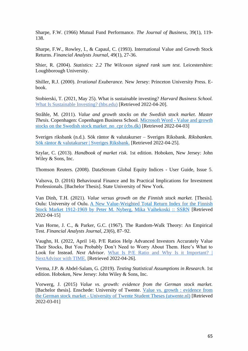
65

Sharpe, F.W. (1966) Mutual Fund Performance. The Journal of Business, 39(1), 119-

138.

Sharpe, F.W., Rowley, I., & Capaul, C. (1993). International Value and Growth Stock

Returns. Financial Analysts Journal, 49(1), 27-36.

Shier, R. (2004). Statistics: 2.2 The Wilcoxon signed rank sum test. Leicestershire:

Loughborough University.

Shiller, R.J. (2000). Irrational Exuberance. New Jersey: Princeton University Press. E-

book.

Stobierski, T. (2021, May 25). What is sustainable investing? Harvard Business School.

What Is Sustainable Investing? (hbs.edu) [Retrieved 2022-04-20].

Stråhle, M. (2011). Value and growth stocks on the Swedish stock market. Master

Thesis. Copenhagen: Copenhagen Business School. Microsoft Word - Value and growth

stocks on the Swedish stock market_no_cpr (cbs.dk) [Retrieved 2022-04-03]

Sveriges riksbank (n.d.). Sök räntor & valutakurser – Sveriges Riksbank. Riksbanken.

Sök räntor & valutakurser | Sveriges Riksbank. [Retrieved 2022-04-25].

Szylar, C. (2013). Handbook of market risk. 1st edition. Hoboken, New Jersey: John

Wiley & Sons, Inc.

Thomson Reuters. (2008). DataStream Global Equity Indices - User Guide, Issue 5.

Valsova, D. (2016) Behavioural Finance and Its Practical Implications for Investment

Professionals. [Bachelor Thesis]. State University of New York.

Van Dinh, T.H. (2021). Value versus growth on the Finnish stock market. [Thesis].

Oulu: University of Oulu. A New Value-Weighted Total Return Index for the Finnish

Stock Market 1912-1969 by Peter M. Nyberg, Mika Vaihekoski :: SSRN [Retrieved

2022-04-15]

Van Horne, J. C., & Parker, G.C. (1967). The Random-Walk Theory: An Empirical

Test. Financial Analysts Journal, 23(6), 87–92.

Vaughn, H. (2022, April 14). P/E Ratios Help Advanced Investors Accurately Value

Their Stocks, But You Probably Don’t Need to Worry About Them. Here’s What to

Look for Instead. Next Advisor. What Is P/E Ratio and Why Is it Important? |

NextAdvisor with TIME. [Retrieved 2022-04-26].

Verma, J.P. & Abdel-Salam, G. (2019). Testing Statistical Assumptions in Research. 1st

edition. Hoboken, New Jersey: John Wiley & Sons, Inc.

Vorwerg, J. (2015) Value vs. growth: evidence from the German stock market.

[Bachelor thesis]. Enschede: University of Twente. Value vs. growth : evidence from

the German stock market - University of Twente Student Theses (utwente.nl) [Retrieved

2022-03-01]

66

Worthington, A. C., & Higgs, H. (2003). Weak-form market efficiency in European

emerging and developed stock markets. [Discussion Paper]. Brisbane: Queensland

University of Technology.

Yang, Z. (2021) Analysis on CAPM and Sharpe ratio in Market investment. Alantis

Press, 166(1), 5-8.

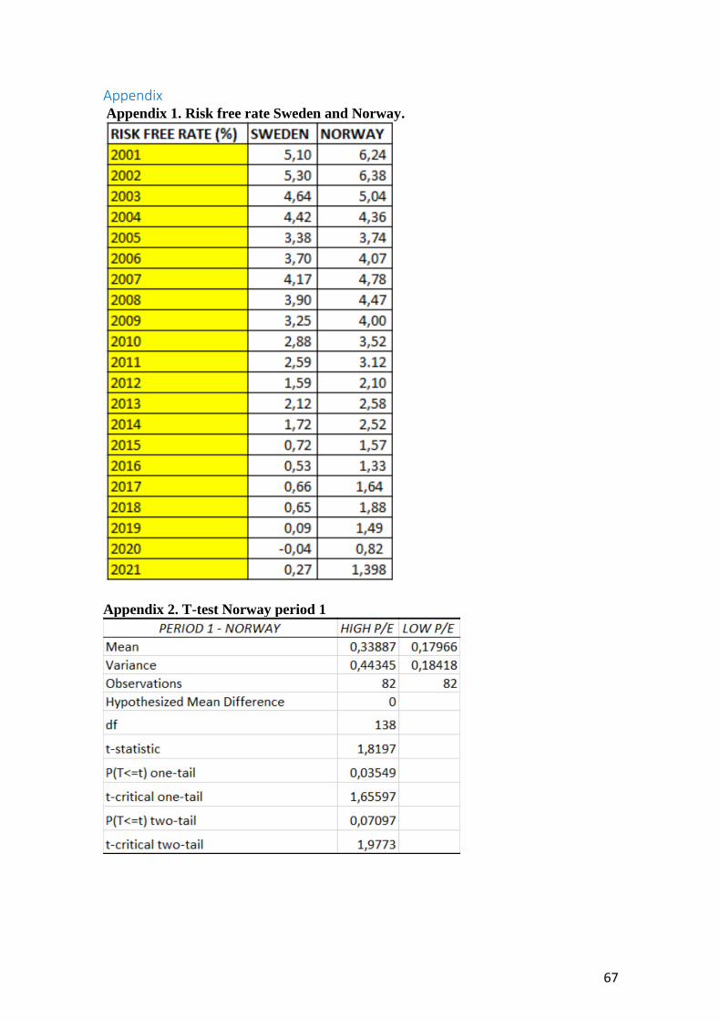
67

Appendix Appendix 1. Risk free rate Sweden and Norway.

Appendix 2. T-test Norway period 1

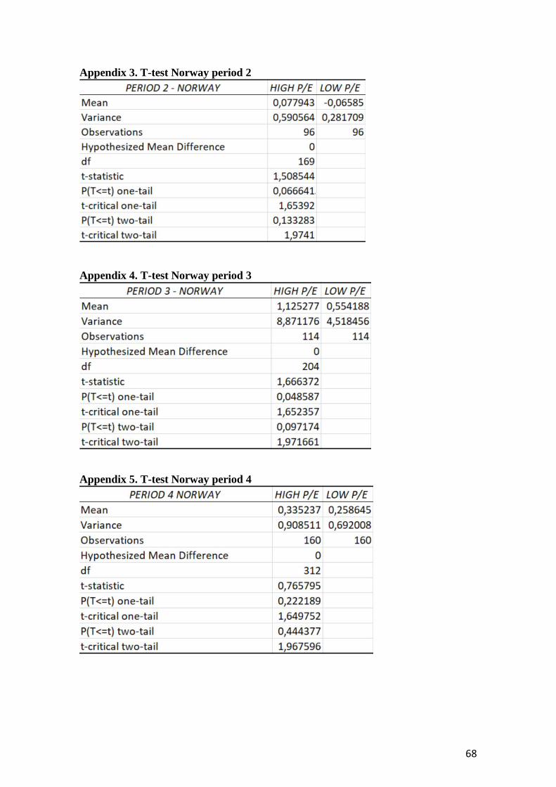
68

Appendix 3. T-test Norway period 2

Appendix 4. T-test Norway period 3

Appendix 5. T-test Norway period 4

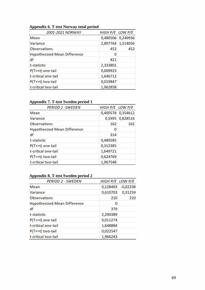
69

Appendix 6. T-test Norway total period

Appendix 7. T-test Sweden period 1

Appendix 8. T-test Sweden period 2

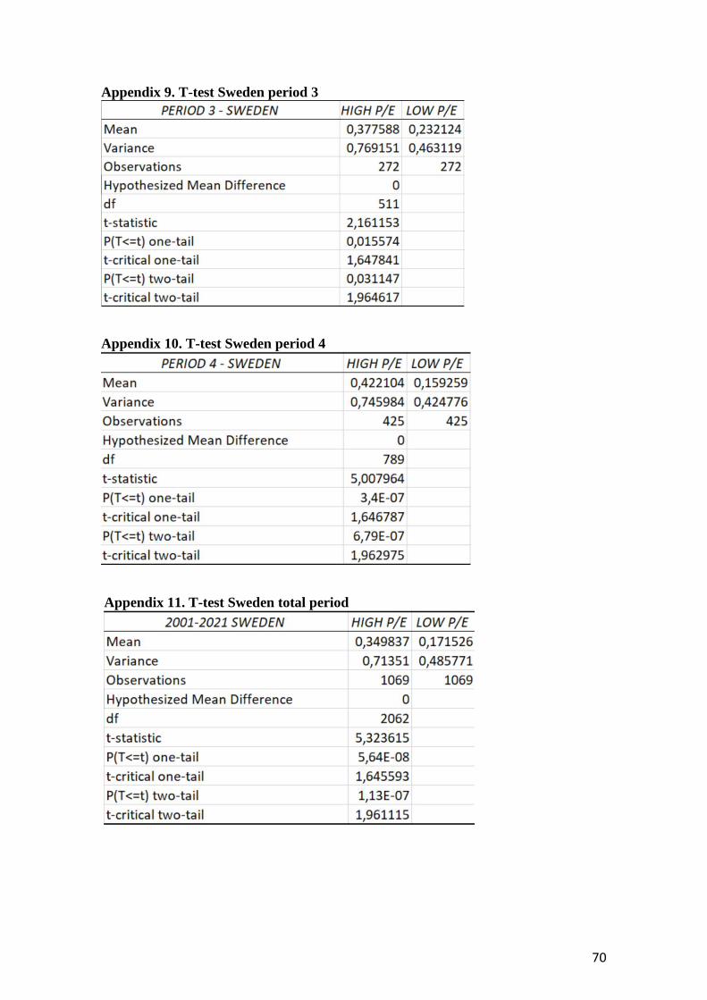
70

Appendix 9. T-test Sweden period 3

Appendix 10. T-test Sweden period 4

Appendix 11. T-test Sweden total period

71