DoD Software Factbook - Carnegie Mellon University · Production Rate ... Mission-Support (MS) Software ... DoD Software Factbook Software Resources Data Report . Distribution Statement

DoD Software Factbook Software Engineering Measurement and Analysis Group Version 1.1

December 2015

Bradford Clark James McCurley David Zubrow

© 2015 Carnegie Mellon University Distribution Statement A: Approved for Public Release; Distribution is Unlimited

DoD Software Factbook

Distribution Statement A: Approved for Public Release; Distribution is Unlimited 1

Copyright 2015 Carnegie Mellon University This material is based upon work funded and supported by the Department of Defense under Contract No. FA8721-05-C-0003 with Carnegie Mellon University for the operation of the Software Engineering Institute, a federally funded research and development center. Any opinions, findings and conclusions or recommendations expressed in this material are those of the author(s) and do not necessarily reflect the views of the United States Department of Defense. This report was prepared for the SEI Administrative Agent AFLCMC/PZM 20 Schilling Circle, Bldg 1305, 3rd floor Hanscom AFB, MA 01731-2125 NO WARRANTY. THIS CARNEGIE MELLON UNIVERSITY AND SOFTWARE ENGINEERING INSTITUTE MATERIAL IS FURNISHED ON AN “AS-IS” BASIS. CARNEGIE MELLON UNIVERSITY MAKES NO WARRANTIES OF ANY KIND, EITHER EXPRESSED OR IMPLIED, AS TO ANY MATTER INCLUDING, BUT NOT LIMITED TO, WARRANTY OF FITNESS FOR PURPOSE OR MERCHANTABILITY, EXCLUSIVITY, OR RESULTS OBTAINED FROM USE OF THE MATERIAL. CARNEGIE MELLON UNIVERSITY DOES NOT MAKE ANY WARRANTY OF ANY KIND WITH RESPECT TO FREEDOM FROM PATENT, TRADEMARK, OR COPYRIGHT INFRINGEMENT. This material has been approved for public release and unlimited distribution except as restricted below. Internal use:* Permission to reproduce this material and to prepare derivative works from this material for internal use is granted, provided the copyright and “No Warranty” statements are included with all reproductions and derivative works. External use:* This material may be reproduced in its entirety, without modification, and freely distributed in written or electronic form without requesting formal permission. Permission is required for any other external and/or commercial use. Requests for permission should be directed to the Software Engineering Institute at [email protected].

* These restrictions do not apply to U.S. government entities. Carnegie Mellon® is registered in the U.S. Patent and Trademark Office by Carnegie Mellon University. DM-0002750

DoD Software Factbook


Contents

Executive Summary ............................................................................ 3

Software Resources Data Report ........................................................ 3

Reporting Frequency ....................................................................... 4

Portfolio Description ........................................................................... 5

Data Age ......................................................................................... 5

Reported Software Process Maturity Levels ................................... 5

Distribution by Super Domain ........................................................ 6

Distribution by Operating Environment ......................................... 6

Team Size........................................................................................ 7

Project Size ..................................................................................... 8

Software Growth Summary ............................................................ 9

Most and Least Expensive Software ................................................. 10

Unit Cost ....................................................................................... 10

Production Rate ............................................................................. 11

Cost Comparison ........................................................................... 12

Effort–Schedule Tradeoff ................................................................. 13

Team Size...................................................................................... 13

Project Size ................................................................................... 13

Average Effort .............................................................................. 14

Average Duration .......................................................................... 14

Tradeoff Results ............................................................................ 15

Best in Class / Worst in Class ........................................................... 16

Analysis Approach ....................................................................... 16

Real-Time (RT) Software ............................................................. 17

Engineering (ENG) Software ....................................................... 19

Mission-Support (MS) Software .................................................. 20

Automated Information System (AIS) ......................................... 21

Conclusions and Next Steps ............................................................. 22

Appendix .......................................................................................... 23

Acronyms & Definitions .............................................................. 23

Equivalent Source Lines of Code (ESLOC) ................................. 24

Super Domains ............................................................................. 25

Operating Environments ............................................................... 26

Transforming Data ........................................................................ 27

This research is funded by the Associate Director for Software Technologies Office of Information Systems & Cyber Security RD / ASD(R&E) / AT&L / Department of Defense.

DoD Software Factbook Executive Summary


Executive Summary This DoD Factbook is an initial analysis of software engineering data from the perspective of policy and management questions about software projects. The analysis relies on the DoD’s Software Resources Data Report (SRDR) and other supporting data. The Factbook provides a description of the DoD software portfolio based on the SRDR data. It then addresses the following questions posed to direct a deeper analysis:

1. What is the most expensive software to develop? 2. To what extent can project duration be shortened or recovered by

adding more people? 3. What differences are there between best-in-class and worst-in-

class software projects? The Factbook focuses on the following three analysis areas to answer the questions:

1. The differences in productivity between different classes of projects. This will identify which project classes are more expensive to develop.

Analysis shows that real-time software is at least three times more expensive to develop than the least expensive software, automated information system software.

2. The tradeoff between software development effort and software development duration. This analysis addresses the ramifications of shortening or recovering project duration by adding more people.

Analysis shows that for typical project durations, a 20% reduction in duration costs an additional 36% increase in effort.

3. The differences in effort, schedule, and cost performance between best-, average-, and worst-in-class projects. Analysis shows that best-in-class projects are over two times more efficient than average projects and upwards of five times more efficient than worst-in-class projects.

The Factbook starts with a discussion and overview of the data used in the analysis of these questions. The three analysis areas follow this introductory material.

Software Resources Data Report The Software Resources Data Report (SRDR) is the primary source of data on software projects and their performance. It is a contract data deliverable that formalized the reporting of software metrics data. It consists of the following two forms:

• data report

• data dictionary

It is designed to record both the estimates and actual results of new software developments or upgrades.

The SRDR applies to all major contracts and subcontracts, regardless of contract type, for contractors developing or producing software elements within Acquisition Category (ACAT) I and IA programs and pre-Major Defense Acquisition Program (MDAP) and pre- Major Automated Information System (MAIS) programs subsequent

DoD Software Factbook Software Resources Data Report


to Milestone A approval for any software development element with a projected software effort greater than $20M.1

Reporting Frequency Programs submit reports for these two types of reporting events:

• Contract event: an SRDR is required at contract start (Initial Developer Report) and at contract completion (Final Developer Report).

• Product event: an SRDR is required at the start of a product increment (Initial Developer Report) and at the completion of a product increment (Final Developer Report). An increment is a partial delivery of a product capability. Increments are also referred to as spirals, builds, and releases.

The report for the start and end of a contract event will contain all of the data for all product events within the contract. Therefore, care must be taken to analyze only records that are from either contract events or product events, but not both.

The SRDR event data used in this analysis is based on product event data and is referred to as project data in this Factbook.

The SRDR data used in this analysis is based on the final report that contains actual result data. Data for this analysis had to include the following information:

• size data

• effort data

• schedule data

1 CSDR Requirements, OSD Defense Cost and Resource Center, http://dcarc.cape.osd.mil/CSDR/CSDROverview.aspx#Introduction

Based on this criterion, the dataset for this analysis used 208 projects from the product-event final-report data.

As more data is added to the Defense Automated Cost Information Management System (DACIMS), this analysis will be expanded and updated.

DoD Software Factbook Portfolio Description


Portfolio Description Data Age The age of the data was derived from the Report as of Date. Submission dates in the analysis dataset of the Final Developer Report range from October 2004 to September 2011. As Figure 1 shows, there are a few projects in 2004. Most of the projects are from the 2008 to 2010 timeframe.

Reported Software Process Maturity Levels In Figure 2, the histogram shows the reported process maturity levels in the analysis dataset. Most projects reported the highest level of maturity. The following are the counts at each maturity level:

• level 3 (64)

• level 4 (24)

• level 5 (119)

Figure 1. Project Distribution for Data Age

Figure 2. Project Distribution for Process Maturity Level

Oct-11Oct-10Oct-09Oct-08Oct-07Oct-06Oct-05Oct-04

16

14

12

10

8

6

4

2

0

Final Report As Of Date

Perc

ent

543

60

50

40

30

20

10

0

Process Maturity Level

Perc

ent



Distribution by Super Domain The analysis dataset can be segregated into different classes called super domains. Super domains are high-level groupings of software application domains, as shown in Figure 3. The four super domains are

• ENG: engineering software (88)

• RT: real-time software (61)

• MS: mission support software (38)

• AIS: automated information system software (21) The four super domains are used later for the best-in-class and worst-in-class analysis. A more detailed explanation of the super domains is provided in the Appendix, Super Domains.

Distribution by Operating Environment The analysis dataset can also be grouped into the operating environments (OpEnv) in which the software operates, as shown in Figure 4. The most dominant environment was ground site followed by aerial vehicle.

• GS: ground site (99)

• AV: aerial vehicle (66)

• GV: ground vehicle (28)

• MV: maritime vessel (11)

• OV: ordnance vehicle (9)

• SV: space vehicle (1)

Examples of these environments are provided in the Appendix, Operating Environments.

Figure 4. Project Distribution by Operating Environment

Figure 3. Project Distribution by Super Domain

SVOVMVGVAVGS

50

40

30

20

10

0

Operating Environment

Perc

ent

AISMSRTENG

40

30

20

10

0

Super Domain

Perc

ent



Team Size The size of development teams is based on measures of project effort and duration. The effort for a project is reported in labor hours. Labor hours are converted to person months (PM) of effort and divided by months of project durations to derive the average level of project staffing.

Figure 5 shows that most teams have 10 or fewer people. Recall that SRDRs are required for contracts over $20M. These contracts have multiple product events resulting in seemingly small team sizes which, in fact, are due to low levels of effort over relatively long durations

Figure 5 also shows the data skewed to the left in the chart’s horizontal axis. This indicates that the data has a non-normal distribution that must be corrected before analyzing team size based on central tendency. Figure 6 shows the log-transformed data and its near-normal distribution. See Appendix, Transforming Data, for more discussion on the significance of normal versus non-normal data distribution.

As will be seen in the Effort-Schedule Tradeoff analysis, project data has to be divided into three team-size groups: small, medium, and large. Projects in these groups are selected from one-third partitioning of a descending-order list of team sizes for projects.

• small-size teams 1 to 3.5 average staff

• medium-size teams 3.6 to 10 average staff

• large-size teams Over 10 average staff

In Figure 6, which shows team size on a log scale, the divisions between small to medium and medium to large are at 0.54 and 1.0, respectively, as depicted by the bold lines.

Figure 6. Project Distribution of FTE – Log Scale

Figure 5. Project Distribution of FTEs

706050403020100

Median

Mean

1210864

1st Quartile 2.683Median 5.7683rd Quartile 12.743Maximum 74.550

8.419 12.359

4.754 6.897

11.874 14.677

A-Squared 16.84P-Value < 0.005

Mean 10.389StDev 13.127Variance 172.307Skewness 2.45790Kurtosis 6.48006N 173

Minimum 0.136

Anderson-Darling Normality Test

95% Confidence Interval for Mean

95% Confidence Interval for Median

95% Confidence Interval for StDev

95% Confidence Intervals

Full Time Equivalent

2.01.61.20.80.40.0-0.4-0.8

Median

Mean

0.850.800.750.700.65


0.63322 0.80186

0.67705 0.83865

0.50825 0.62824

A-Squared 1.07P-Value 0.008

Mean 0.71754StDev 0.56187Variance 0.31570Skewness -0.484540Kurtosis 0.184375N 173

Minimum -0.86774






Full Time Equivalent - Log Transformed



Project Size This analysis uses a product-size measure based on software source lines of code (SLOC). A key issue in using SLOC as a measure of work effort and duration is the difference in work required to incorporate software from different sources, including:

• new code

• modified code (changed in some way to make it suitable)

• reused code (used without changes)

• auto-generated code (created from a tool and used without change)

Each of these computer-code sources requires a different amount of work effort to incorporate into a software product. The challenge is in coming up with a single measure that includes all of the code sources.

The approach taken is to normalize all code sources to the equivalent of a new line of code. This is done by taking a portion of the measures for modified, reused, and auto-generated code. The portioning is based on the percentage of modification to the code based on changes to the design, code, and unit test, and integration and test documents. This is further explained in the Appendix, Equivalent Source Lines of Code.

Figure 7 shows that most projects have a size less than 80,000 equivalent source lines of code (ESLOC) with an average size of 57,199 ESLOC and a median size of 28,598. When the size data is transformed (Figure 8) into a more normal-like distribution, the average project size is 104.37 or 23,442 ESLOC and the median is 104.46 or 28,840 ESLOC.

As an easy heuristic, the average project size is around 25,000 ESLOC for all projects.

Figure 7. Project Distribution of Size

5.44.84.23.63.02.4

Median

Mean

4.554.504.454.404.354.30


4.2764 4.4531

4.3086 4.5496

0.5958 0.7214


Mean 4.3647StDev 0.6526Variance 0.4258Skewness -0.315464Kurtosis -0.492187N 212

Minimum 2.4803






Equivalent Source Lines of Code - Log Trans.

Figure 8. Project Distribution of Size – Log Scale

480000400000320000240000160000800000

Median

Mean

700006000050000400003000020000

1st Quartile 6899Median 285983rd Quartile 72219Maximum 475254

46404 67994

20351 35450

72798 88142


Mean 57199StDev 79734Variance 6357456546Skewness 2.64418Kurtosis 8.36081N 212

Minimum 302






Equivalent Souce Lines of Code



Software Growth Summary Table 1 shows the change in software size and total hours of effort for all available record pairings of an initial SRDR and a corresponding final SRDR. The initial SRDR reports an estimate and the final SRDR reports the actual value. In Table 1, growth is shown in a pair of rows for each of the measures. The first row shows the growth in terms of the measure itself and the second row shows the growth in terms of percentage of change.

Both ESLOC and effort change have wide variation from project to project and display skewed distributions. In these cases, the median—or 50th percentile—provides a better indication of the typical magnitude of change from the initial to final values. The median figures of percentage change provide a normalized indication of the magnitude of change. For ESLOC the median growth is 27% and for effort the growth is 19%. The skewness and spread of these distributions is graphically depicted in Figure 9 and Figure 10.

Table 1. Change in Software Size and Hours of Effort

Variable N Median

Change in ESLOC 190 4,304

Percentage Change in ESLOC

190 27%

Change in Total Hours 190 5,584

Percentage Change in Total Hours

189 19%

Figure 10. Project Distribution of %Change in Hours of Effort

Figure 9. Project Distribution of %Change in Software Size

1800.00%1500.00%1200.00%900.00%600.00%300.00%0.00%

Median

Mean

120.00%100.00%80.00%60.00%40.00%20.00%0.00%

1st Quartile -0.0667Median 0.27023rd Quartile 0.9432Maximum 17.8224

0.5346 1.1930

0.1282 0.3680

2.0898 2.5580



Minimum -0.8956




95% Confidence Interval for StDev95% Confidence Intervals

Summary for ΔESLOC%

DoD Software Factbook Most and Least Expensive Software


Most and Least Expensive Software What is the most expensive software to develop? The analysis is based on the rationale that some types of software are more difficult to develop than other types and therefore require more effort to develop. The level of difficulty can be caused by factors such as execution timing constraints, interoperability requirements, commercial-off-the-shelf (COTS) software product incorporation, algorithmic complexity, communication complexity, data-bandwidth requirements, security requirements, and so forth. To account for the dissimilarities in project difficulty, projects are segregated into four groups based on their super domains.

Two cost-related concepts are used in this analysis: unit cost and production rate.

• Unit cost is the cost of producing a unit of software with some amount of effort. In this case, the unit of software is thousands of ESLOC (KESLOC). The effort is person months, which can be translated into cost using an average labor rate.

• Production rate is the rate at which a unit of software is delivered over a period of time. The unit of software is ESLOC and the time is months of project duration.

To get a complete picture of software cost, unit cost should be normalized with the production rate. This is done because some projects may choose to employ more staff to increase their production rate and deliver the software faster.

Unit Cost With an average project size of 25,000 ESLOC, each of the four groups are displayed in the scatter-plot chart, Figure 11. Trend lines run through the average of each group. The black vertical line is a reference for the average project size discussed earlier.

The trend lines on the chart show that there are differences in unit costs between the four groups. The trend line for real-time software shows that for small amounts of size, a large amount of effort is required; that is, real-time software has a high unit cost. The trend line for automated information system software shows the opposite: for large amounts of size, a small amount of effort is required.

Apart from the implications of the trend lines, it is difficult to tell what is happening with the average project size of 25,000 ESLOC. If the data is transformed to a log scale, the comparisons become easier to discern.

The scatter-plot chart in Figure 12 is a log-transformed version of Figure 11. Its transformation makes it easier to see the relationships between the four groups for an average project size. The order of unit costs (from highest to lowest) for an average-size project is as follows:

0

500

1,000

1,500

2,000

2,500

3,000

3,500

4,000

0 100 200 300 400 500

Pers

on M

onth

s

KESLOCRT ENG MS AIS

Figure 11. Unit Cost Scatter Plot



• real-time software 12.2 PM per KESLOC • engineering software 8.8 PM per KESLOC • mission support software 5.1 PM per KESLOC • automated information system 2.8 PM per KESLOC

Production Rate The scatter-plot chart for the production rate, using a data-transformed log scale, is shown in the second chart to the right. This chart shows the relationships between the four groups for how long it takes to deliver a unit of software. For an average-size project, the order of production rate is as follows:

• real-time software 1.5 months per KESLOC • engineering software 1.3 months per KESLOC • mission support software 1.3 months per KESLOC • automated information system 1.1 months per KESLOC

Care must be taken when making comparisons for projects of other sizes. As can be seen in Figure 12 and Figure 13, the trend lines intersect, indicating that the orderings of unit cost and production rate vary with size. For instance, in the smaller size range, the data show that the unit cost of RT software is slightly less than that for ENG software. A similar result is shown by the trend line for MS software in terms of production rate.

1

10

100

1000

0.1 1 10 100 1000

Mon

ths

KESLOCAIS ENG MS RT 25K

Figure 13. Production Rate Scatter Plot - Log Scale

1

10

100

1,000

10,000

0.1 1 10 100 1000

Pers

on M

onth

s

KESLOCRT ENG MS AIS

Figure 12. Unit Cost Scatter Plot - Log Scale



Cost Comparison The average number of staff each month can be determined when unit cost is normalized with production rate. Assuming an average annual burden labor cost2 of $150,000/staff, the normalized monthly cost for each group is shown:

• real-time software 8.1 people or $101,250 • engineering software 6.7 people or $83,750 • mission support software 3.9 people or $48,750 • automated information system 2.5 people or $31,250 Real-time software is the most expensive to develop and automated information system software is the least expensive.

2 Annual burden labor rate includes wages, payroll taxes, worker's compensation and health insurance, paid time off, training and travel expenses, vacation and sick leave, pension contributions, and other benefits. It may be as much as 50% higher

than payroll costs alone. A $150,000 average annual burden labor rate breaks down to $12,500/month and $82.24/hour using 1,824 labor hours in a year

DoD Software Factbook Effort–Schedule Tradeoff


Effort–Schedule Tradeoff Can project duration be shortened or recovered by adding more people? The approach for this analysis is to look at the increase in the percent of effort required to reduce a percentage of schedule or duration. The simple strategy of reducing schedule 20% by increasing effort 20% may work in manufacturing, but does it work in software development?

Team Size In small-size teams, effort and schedule are heavily influenced by individuals. Larger teams experience an averaging effect among team members for influencing effort and schedule. Since this analysis is attempting to draw conclusions based on averages, medium- and large-team-size projects are examined for the tradeoff between effort and time. Recall from the earlier discussion on team size:

• medium-size teams 3.6 to 10 average staff

• large-size teams over 10 average staff

In Figure 14, the blue cloud represents medium-size projects and the red cloud represents large-size projects.

Project Size An average project size is also needed for this analysis for comparison of effort and duration between the two team sizes. The average project size based on medium and large team size is 50,000 ESLOC. See the black vertical bar in the chart.

1.0

10.0

100.0

100 1,000 10,000 100,000 1,000,000

Aver

age

Staf

fing

ESLOC

Figure 14. Comparison of Medium- vs. Large-Team Software Size



Average Effort Figure 15 shows the difference in effort between using medium- and large-size teams. A red trend line for a medium-size team and a blue trend line for a large-size team representing the average effort expended per ESLOC are shown. A black line for an average 50,000 ESLOC project intersects the red and blue lines.

The effort expended on an average-size project by each team is as follows:

• medium-size team 258 person months • large-size team 455 person months

The difference in effort between the medium and large team is 197 person months of effort. This difference is attributed to the different development durations for each team and is discussed next.

Average Duration Figure 16 shows the difference in development time between using medium- and large-size teams. The time it takes each team to finish an average-size project is as follows:

• medium-size team 43 months

• large-size team 25 months

The difference in development time between the medium- and large-size teams is 18 months.

As expected, medium-size teams expend less effort and take longer for an average-size project. Larger size teams perform the reverse. But what is the tradeoff between increasing effort and reducing schedule?

10

100

1000

10000

100 1,000 10,000 100,000 1,000,000

Pers

on M

onth

s

ESLOCMedium Size Teams Large Size Teams

1

10

100

1000

100 1,000 10,000 100,000 1,000,000

Mon

ths

ESLOCMedium Size Teams Large Size Teams

Figure 15. Comparison of Medium- vs. Large-Team Development Effort

Figure 16. Comparison of Medium- vs. Large-Team Development Duration



Tradeoff Results The time to develop an average-size project was reduced from 43 to 25 calendar months, a 42% reduction. This came at the expense of increasing effort from 258 to 455 person months, a 76% increase. For each 1% reduction in schedule, there is a 1.8% increase in effort.

Instead of achieving a 20% reduction in schedule with a 20% increase in effort, as stated in the manufacturing example earlier, a 50,000 ESLOC project would reduce schedule 20% by adding 36% more effort. The strategy of reducing or reclaiming schedule by increasing the number of people on a project is expensive. It is also non-linear (the charts shown in this analysis are in log scale, meaning the trend lines are curved and not straight); that is, a larger percentage of schedule reduction is accompanied by a disproportionately larger percentage increase in effort.

These results corroborate the schedule-compression driver in the COCOMO II model.3 In that model, a 15% schedule reduction causes a 14% increase in effort. A 25% schedule reduction causes a 43% increase in effort. The analysis presented here shows that a 20% schedule reduction causes a 36% increase in effort.

Project size does not appear to be the only factor that drives the amount of effort on a project. Schedule compression also has a significant impact on staffing level.

3 Boehm, B., Abts, C., Brown, W, Chulani, S., Clark, B., Horowitz, E., Madachy, R., Reifer, R., and Steece, B., “Software Cost Estimation with COCOMO II,” Prentice Hall, Upper Saddle River, NJ, 2000, pp. 50-51.

DoD Software Factbook Best in Class / Worst in Class


Best in Class / Worst in Class What differences are there between best-in-class and worst-in-class software projects? To assess differences between projects, two derived metrics are used: efficiency and speed. Efficiency is a measure of how much product can be produced per unit of effort. In this analysis, the amount of product is expressed as ESLOC. The effort is expressed as the number of people and amount of time required to produce the product, that is, the number of person months of effort. Dollar cost is derived by applying a labor rate to the person-month effort measure.

Speed is a measure of how fast a product can be produced. Again, the amount of product is expressed as ESLOC. Time is expressed as calendar months.

The dataset was segregated and analyzed in four classes based on the super domains discussed earlier: real-time, engineering, mission support, and automated information software. See Appendix, Super Domains for definitions of each super domain.

Analysis Approach The analysis uses projects separated by their super domain or class. The focus is on an average project size of 25,000 ESLOC (as discussed earlier) within each class. Using a project of average size, project efficiency and speed are derived. A ±1 standard deviation (SD) about the efficiency and speed average are used to categorize best and worst projects. One standard deviation above and below the mean includes about 67% of projects, and therefore about 1/6th of the projects are deemed to be in the best and in the worst categories.

4 Burden labor rate includes wages, payroll taxes, worker's compensation and health insurance, paid time off, training and travel expenses, vacation and sick

The assignment into the best-in-class and worst-in-class categories was done as follows:

• Best: all projects below the −1 SD vale are projects that used less effort or took less time to finish than average.

• Worst: all projects above the +1 SD value are projects that used more effort or took more time to finish than average.

Projects within ±1 standard deviation are deemed average, that is, neither best nor worst-in-class.

Each analysis presents scatter-plot charts for efficiency and speed for each software super domain. The average trend line and ±1 SD are shown, discussed and compared among best, average, and worst in class. An assumed burden labor rate4 of $150 per hour is used to compare costs. A table at the end of the analysis summarizes results.

leave, pension contributions, and other benefits. It may be as much as 50% higher than payroll costs alone.



Real-Time (RT) Software

Efficiency The RT efficiency chart in Figure 17 shows an average trend line through size and effort data for 61 real-time software projects. The average-size project expends 304 person months of effort. Best-in-class projects expend 155 person months of effort, and worst-in-class projects expend 594 person months of effort. The difference between a best- or worst-in-class project from the average is 149 person months. The difference between best and worst in class is 298 person months.

Best-in-class RT projects are almost 2 times more efficient than average projects and 3.8 times more efficient than worst-in-class projects.

Using a burden labor rate of $150,000 per year, the best-in-class project saves $1.863M dollars over an average project and $3.725M over a worst-in-class project.

Speed The average-size project delivers a product in 38 months. A best-in-class project delivers a product in 21 months. And a worst-in-class project delivers a product in 69 months, as shown in Figure 18. Best-in-class projects are 1.8 times faster than average projects and 3.3 times faster than worst in class.

Figure 17. Real-Time Software Efficiency

1

10

100

1000

10000

100 1,000 10,000 100,000 1,000,000

Pers

on M

onth

s

ESLOC

Figure 18. Real-Time Software Speed

1.0

10.0

100.0

100 1,000 10,000 100,000 1,000,000

Mon

ths

ESLOC



Table 2 summarizes the differences in efficiency and speed between best, average, and worst-in-class RT projects.

Table 2. Real-Time Software Best & Worst Summary

Metric Best in Class Average

Worst in Class

Effort (Person Months) 155 304 594

Schedule (Months) 21 38 69

Cost (Millions) $1.938 $3.800 $7.425



Engineering (ENG) Software

Efficiency There are 92 projects in the ENG super domain. The average-size project expends 215 person months of effort. The best-in-class expends 93 person months, and the worst in class expends 496 person months, as shown in Figure 19. The best-in-class project is 2.3 times more efficient than average projects and 5.3 times more efficient than worst-in-class projects.

Using a burden labor rate of $150,000 per year, the best-in-class project saves $1.525M dollars over an average project and $5.038M dollars over a worst-in-class project.

Speed The average-size best-in-class project delivers a software product in 19 months, an average project in 32 months, and a worst-in-class project in 55 months, as shown in Figure 20. The best-in-class project is 1.7 times faster than an average project and 2.9 times faster than a worst-in-class project.

Table 3 summarizes the differences in efficiency and speed between best, average, and worst-in-class ENG projects.

1

10

100

1000

10000

100 1,000 10,000 100,000 1,000,000

Pers

on M

onth

s

ESLOC

Table 3. Engineering Software Best & Worst Summary

Metric Best-in-Class Average

Worst-in- Class



Cost (Millions) $1.163 $2.688 $6.200

Figure 19. Engineering Software Efficiency

Figure 20. Engineering Software Speed

1.0

10.0

100.0

1000.0

100 1,000 10,000 100,000 1,000,000

Mon

ths

ESLOC



Mission-Support (MS) Software

Efficiency The mission-support super domain has 38 projects. The best-in-class, average, and worst-in-class projects expended 52, 127, and 306 person months, respectively, as shown in Figure 21. A best-in-class project is 2.4 times more efficient than an average project and 5.8 times more efficient than a worst-in-class project.

Best-in-class projects save $926K dollars over average projects and $3.163M dollars over worst-in-class projects using a burden labor rate of $150 per hour.

Speed Product delivery is 20 months for an average-size, best-in-class project. Average projects take 33 months. Worst-in-class projects take 56 months, as shown in Figure 22. This means best-in-class projects are 1.7 times faster than average projects and 2.8 times faster than worst-in-class projects.

Table 4 summarizes the differences in efficiency and speed between best, average, and worst MS software projects.

Figure 21. Mission Support Software Efficiency

1

10

100

1000

10000

100 1,000 10,000 100,000 1,000,000

Pers

on M

onth

s

ESLOC

1.0

10.0

100.0

1000.0

100 1,000 10,000 100,000 1,000,000

Mon

ths

ESLOC

Table 4. Mission Support Software Best & Worst Summary


Worst in Class



Cost (Millions) $0.662 $1.588 $3.825

Figure 22. Mission Support Software Speed



Automated Information System (AIS)

Efficiency Using a project size of 75,000 ESLOC,5 best-in-class, average, and worst-in-class projects expended an average of 147, 207, and 293 person months of effort, respectively (see Figure 23). That makes best-in-class projects 1.4 times more efficient than average projects and almost 2 times more efficient than a worst-in-class project.

Best-in-class projects save $250K over average projects and $588K over worst-in-class projects for an average-size project.

Speed Best-in-class projects deliver a software product 2 times faster than average projects and 4.3 times faster than worst-in-class projects (see Figure 24).

Table 5 summarizes the differences in efficiency and speed between best, average, and worst AIS software projects.

5 The change in project size from the previous average of 25,000 to 75,000 ESLOC is due to the removal of two project outliers with sizes one order of magnitude less

than the other projects in this class. These outliers disproportionately influenced the results.

Table 5. AIS Software Best & Worst Summary


Worst in Class



Cost (Millions) $0.625 $0.875 $1.213

Figure 23. AIS Software Efficiency

Figure 24. AIS Software Speed

1.0

10.0

100.0

1000.0

10,000 100,000 1,000,000

Mon

ths

ESLOC

AIS-Speed

1

10

100

1000

10000

10,000 100,000 1,000,000

Pers

on M

onth

s

ESLOC

AIS-Efficiency

DoD Software Factbook Conclusions and Next Steps


Conclusions and Next Steps This analysis shows that the cost of software development varies depending on several factors. All of the charts that show size versus effort imply that as the size of a software project increases, there is a corresponding increase in the amount of development effort (an indicator of labor cost). But size is not the lone determiner of cost.

The class or super domain of software makes a difference in the cost of software. Different super domains have different levels of difficulty that cause more effort to be expended on more difficult software. On an average-size project, automated information system software costs $31,350 a month and real-time software costs $101,250 a month, more than three times as much.

The time it takes to develop software also drives cost. Based on an average-size project, shorter duration projects cost disproportionately more than longer duration projects. It was shown that team size is clearly not determined solely by the size of the software to be built.

The effort-schedule tradeoff analysis result also implies that projects with slipping milestones will require disproportionately more effort when attempts are made to recover schedule.

The performance of a project also drives cost. The analysis looked at best, average, and worst performing projects within each super domain. Unfortunately there was not enough background data on projects to investigate why best and worst projects perform differently. This leads to the next steps.

There is an effort to link the project data back to source documents and other data to make it possible to investigate the data more fully. There is a lot of data and source material, and some progress has been made to date with a lot more to do.

There is additional SRDR data that can be added to this analysis, and new data is submitted every quarter. More data would increase the

fidelity of grouping the data into different super domains of software, providing a more robust analysis.

The intent of this report is to provide a characterization of the DoD software portfolio and to demonstrate how the SRDR data is useful in gaining insights into software-development costs. More analysis can be done, but we want to ask you, “What are the important questions that need answers?” We would like to receive feedback on this report and input for useful extensions. For comments and suggestions, please contact [email protected]

Thank you.

mailto:[email protected]

DoD Software Factbook Appendix


Appendix Acronyms & Definitions AIS automated information system software (See

Appendix, Super Domains.)

DACIMS Defense Automated Cost Information Management System

ENG engineering software (See Appendix, Super Domains.)

ESLOC equivalent source lines of code. (See Appendix, Equivalent Source Lines of Code.)

FTE full-time equivalent; the number of total hours worked divided by the maximum number of compensable hours in a full-time schedule. For example, if the normal schedule for a quarter is defined as 35 hours per week * (52 weeks per year / 4), 411.25 hours, then someone working 100 hours during that quarter represents 100/411.25 = 0.24 FTE.

KESLOC thousands (K) of ESLOC

MAIS Major Automated Information System

MDAP Major Defense Acquisition Program

MS mission-support software (See Appendix, Super Domains.)

OpEnv operating environment (See Appendix, Operating Environment.)

PD person days; a measure of effort based on eight hours per day for requirements through final qualification testing activities; 1 PD = 1 calendar day only when one person is working on the project.

PM person months; a measure of effort based on an average of 152 labor hours in a month. The average includes vacation time, sick time, and holidays.

project data data from an SRDR product event

RT real-time software systems (See Appendix, Super Domains.)

SD standard deviation; the amount of variation in the data. ±1 standard deviation covers about 67% of projects.

SRDR Software Resources Data Report



Equivalent Source Lines of Code (ESLOC) A key issue in using software source lines of code (SLOC) as a measure of work effort and duration is the difference in work required to incorporate software from different sources: new code, modified code (changed in some way to make it suitable), reused code (used without changes), and auto-generated code (created from a tool and used without change). Each of these computer-code sources requires a different amount of work to incorporate into a software product. The challenge is in coming up with a single measure that includes all of the code sources.

The approach taken here is to normalize all code sources to the equivalent of a new line of code. This is done by taking a portion of the measures for modified, reused, and auto-generated code. The portioning is based on the percentage of modification to the code based on changes to the design, code and unit test, and integration and test documents. This approach is adopted from the COCOMO II software cost estimation model.6

Equivalent source lines of code (ESLOC), then, is the homogeneous sum of the different code sources. The portion of each code source is determined using a formula called an adaption adjustment factor (AAF):

AAF = (0.4 x %DM) + (0.3 x %CM) + (0.3 x %IM)

Where

%DM: Percentage Design Modified

%CM: Percentage Code and Unit Test Modified

6 Boehm, B., Abts, C., Brown, W, Chulani, S., Clark, B., Horowitz, E., Madachy, R., Reifer, R., and Steece, B., “Software Cost Estimation with COCOMO II,” Prentice Hall, Upper Saddle River, NJ, 2000, p. 22.

%IM: Percentage Integration and Test Modified

Using a different set of percentages for the different code sources, ESLOC is expressed as

ESLOC = New SLOC + (AAFM x Modified SLOC) + (AAFR x Reused SLOC) + (AAFAG x Auto-Generated SLOC)

• New code does not require any adaption parameters, since nothing has been modified.

• Auto-generated code does not require the DM or CM adaption parameters. However, it does require testing, IM. If auto-generated code does require modification, then it becomes modified code, and the adaptation factors for modified code apply.

• Reused code does not require the DM or CM adaption parameters either. It also requires testing, IM. If reused code does require modification, then it becomes modified code and the adaptation factors for modified code apply.

• Modified code requires the three parameters, DM, CM, and IM, representing modifications to the modified code design, code, and integration testing.

The equivalent sizes for all of the projects are shown in the histogram graphs. The first histogram shows that sizes for the projects do not have a normal distribution. The analyses in this Factbook rely on statistical methods that require a normally distributed dataset.



Super Domains

Real-Time (RT) Real-time is the most complex type of software. These projects take the most time and effort for a given system size due to the lower language levels, high level of abstraction, and increased complexity. Characteristics include

• tightly coupled interfaces

• real-time scheduling requirements

• very high reliability requirements (life critical)

• generally severe memory and throughput constraints

• often executed on special-purpose hardware

Examples of software domains in this super domain are: sensor control and signal processing, vehicle control, vehicle payload, and real-time embedded.

Engineering (ENG) Engineering is a software type of medium complexity. Characteristics include

• multiple interfaces with other systems

• constrained response-time requirement

• high reliability but not life critical

• generally executed on commercial off-the- shelf (COTS) software applications

Examples of software domains in this super domain are: mission processing, executive, automation and process control, scientific systems, and telecommunications.

Mission Support (MS) Mission support is the least complex type of software. Software is often written in more human-oriented languages and performs common business functions such as order entry, inventory, human resources, financial transactions, and data processing and storage. Characteristics include

• relatively less complex

• self-contained or few interfaces

• less stringent reliability requirement

Examples of software domains in this super domain are: planning systems, non-embedded training, software tools, and non-embedded test software

Automated Information Systems (AIS) Automated information systems describes software that automates information processing. These applications allow the designated authority to exercise control over the accomplishment of the mission. Humans manage a dynamic situation and respond to user input in real time to facilitate coordination and cooperation.

Examples of software domains in this super domain are: intelligence and information systems, software services, and software applications.



Operating Environments Aerial Vehicle (AV)

Examples of aerial vehicles are

• manned: fixed-wing aircraft, helicopters

• unmanned: remotely piloted air vehicles Ground Site (GS)

Examples of ground sites are

• fixed: command post, ground operations center, ground terminal, test faculties

• mobile: intelligence-gathering stations mounted on vehicles, mobile missile launcher, handheld devices

Ground Vehicle (GV)

Examples of ground vehicles are

• manned: tanks, howitzers, personnel carrier, mobile missile launcher

• unmanned: robots Maritime Vessel (MV)

Examples of maritime vessels are

• manned: aircraft carriers, destroyers, supply ships, submarines

• unmanned: mine-hunting systems, towed sonar array

Ordnance Vehicle (OV)

Examples of ordnance vehicles are

• air-to-air missiles, air-to-ground missiles, smart bombs, strategic missiles

Space Vehicle (SV)

• manned: passenger vehicle, cargo vehicle, space station

• unmanned: orbiting satellites (weather, communications), exploratory space vehicles



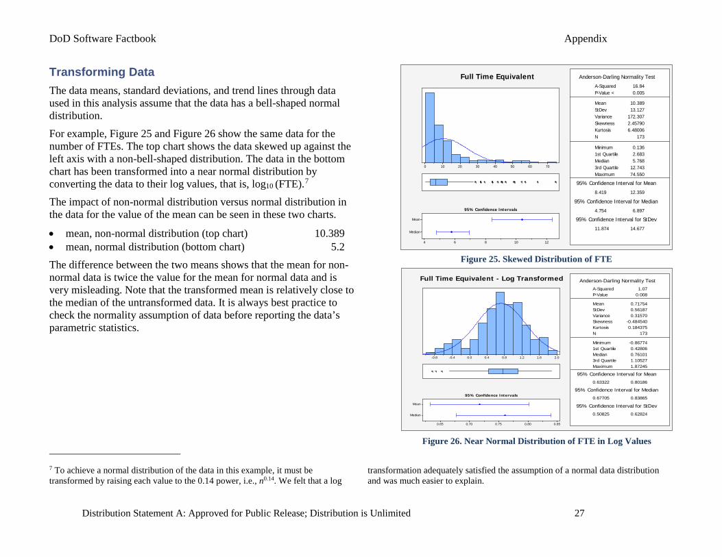
Transforming Data The data means, standard deviations, and trend lines through data used in this analysis assume that the data has a bell-shaped normal distribution.

For example, Figure 25 and Figure 26 show the same data for the number of FTEs. The top chart shows the data skewed up against the left axis with a non-bell-shaped distribution. The data in the bottom chart has been transformed into a near normal distribution by converting the data to their log values, that is, log10 (FTE).7 The impact of non-normal distribution versus normal distribution in the data for the value of the mean can be seen in these two charts.

• mean, non-normal distribution (top chart) 10.389 • mean, normal distribution (bottom chart) 5.2 The difference between the two means shows that the mean for non-normal data is twice the value for the mean for normal data and is very misleading. Note that the transformed mean is relatively close to the median of the untransformed data. It is always best practice to check the normality assumption of data before reporting the data’s parametric statistics.

7 To achieve a normal distribution of the data in this example, it must be transformed by raising each value to the 0.14 power, i.e., n0.14. We felt that a log

transformation adequately satisfied the assumption of a normal data distribution and was much easier to explain.

Figure 26. Near Normal Distribution of FTE in Log Values

Figure 25. Skewed Distribution of FTE

2.01.61.20.80.40.0-0.4-0.8

Median

Mean

0.850.800.750.700.65


0.63322 0.80186

0.67705 0.83865

0.50825 0.62824


Mean 0.71754StDev 0.56187Variance 0.31570Skewness -0.484540Kurtosis 0.184375N 173

Minimum -0.86774






Full Time Equivalent - Log Transformed

706050403020100

Median

Mean

1210864


8.419 12.359

4.754 6.897

11.874 14.677



Minimum 0.136






Full Time Equivalent

DoD Software Factbook - Carnegie Mellon University · Production Rate ... Mission-Support (MS) Software ... DoD Software Factbook Software Resources Data Report . Distribution Statement

Documents