Documentation of Versions 5.0.1, 5.1.0, and 5.2.0

December 2008

NASA/TM–2008–104606, Vol. 27

Technical Report Series on Global Modeling and Data Assimilation, Volume 27

Max J. Suarez, Editor

The GEOS-5 Data Assimilation System—Documentation of Versions 5.0.1, 5.1.0, and 5.2.0

M.M. Rienecker, M.J. Suarez, R. Todling, J. Bacmeister, L. Takacs, H.-C. Liu, W. Gu, M. Sienkiewicz, R.D. Koster, R. Gelaro, I. Stajner, and J.E. Nielsen

The NASA STI Program Offi ce … in Profi le

Since its founding, NASA has been ded i cat ed to the ad vance ment of aeronautics and space science. The NASA Sci en tifi c and Technical Information (STI) Pro gram Offi ce plays a key part in helping NASA maintain this im por tant role.

The NASA STI Program Offi ce is operated by Langley Re search Center, the lead center for NASA̓ s scientifi c and technical in for ma tion. The NASA STI Program Offi ce pro vides ac cess to the NASA STI Database, the largest col lec tion of aero nau ti cal and space science STI in the world. The Pro gram Offi ce is also NASA̓ s in sti tu tion al mech a nism for dis sem i nat ing the results of its research and de vel op ment ac tiv i ties. These results are published by NASA in the NASA STI Report Series, which includes the following report types:

• TECHNICAL PUBLICATION. Reports of com plet ed research or a major signifi cant phase of research that present the results of NASA pro-grams and include ex ten sive data or the o ret i cal analysis. Includes com pi la tions of sig nifi cant scientifi c and technical data and in for ma tion deemed to be of con tinu ing ref er ence value. NASA̓ s counterpart of peer-re viewed formal pro fes sion al papers but has less stringent lim i ta -tions on manuscript length and ex tent of graphic pre sen ta tions.

• TECHNICAL MEMORANDUM. Scientifi c and tech ni cal fi ndings that are pre lim i nary or of spe cial ized interest, e.g., quick re lease reports, working papers, and bib li og ra phies that contain minimal annotation. Does not contain extensive analysis.

• CONTRACTOR REPORT. Scientifi c and techni-cal fi ndings by NASA-sponsored con trac tors and grantees.

• CONFERENCE PUBLICATION. Collected pa pers from scientifi c and technical conferences, symposia, sem i nars, or other meet ings spon sored or co spon sored by NASA.

• SPECIAL PUBLICATION. Scientifi c, tech ni cal, or historical information from NASA pro grams, projects, and mission, often con cerned with sub-jects having sub stan tial public interest.

• TECHNICAL TRANSLATION. En glish-language trans la tions of foreign sci en tifi c and tech ni cal ma-terial pertinent to NASA̓ s mis sion.

Specialized services that complement the STI Pro-gram Offi ceʼs diverse offerings include cre at ing custom the sau ri, building customized da ta bas es, organizing and pub lish ing research results . . . even pro vid ing videos.

For more information about the NASA STI Pro gram Offi ce, see the following:

• Access the NASA STI Program Home Page at http://www.sti.nasa.gov/STI-homepage.html

• E-mail your question via the Internet to [email protected]

• Fax your question to the NASA Access Help Desk at (301) 621-0134

• Telephone the NASA Access Help Desk at (301) 621-0390

• Write to: NASA Access Help Desk NASA Center for AeroSpace In for ma tion 7115 Standard Drive Hanover, MD 21076–1320

National Aeronautics and Space Administration

Goddard Space Flight CenterGreenbelt, Maryland 20771

December 2008

NASA/TM–2008–104606, Vol. 27

Technical Report Series on Global Modeling and Data Assimilation, Volume 27

Max J. Suarez, Editor

The GEOS-5 Data Assimilation System—Documentation of Versions 5.0.1, 5.1.0, and 5.2.0

M.M. Rienecker and M.J. SuarezNASA Goddard Space Flight Center, Greenbelt, Maryland

R. TodlingScience Applications International Corporation, Beltsville, Maryland

J. BacmeisterUniversity of Maryland, Baltimore County, Baltimore, Maryland

L. Takacs, H.-C. Liu, W. Gu, and M. SienkiewiczScience Applications International Corporation, Beltsville, Maryland

R.D. Koster and R. GelaroNASA Goddard Space Flight Center, Greenbelt, Maryland

I. Stajner (former employee)Science Applications International Corporation, Beltsville, Maryland

J.E. NielsenScience Systems and Applications, Inc., Lanham, Maryland

Available from:

NASA Center for AeroSpace Information National Technical Information Service7115 Standard Drive 5285 Port Royal RoadHanover, MD 21076-1320 Springfield, VA 22161

iii

Abstract

This report documents the GEOS-5 global atmospheric model and data assimilation system (DAS), including the versions 5.0.1, 5.1.0, and 5.2.0, which have been implemented in products distributed for use by various NASA instrument team algorithms and ultimately for the Modern Era Retrospective-analysis for Research and Applications (MERRA). The DAS is the integration of the GEOS-5 atmospheric model with the Gridpoint Statistical Interpolation (GSI) Analysis, a joint analysis system developed by the NOAA/National Centers for Environmental Prediction and the NASA/Global Modeling and Assimilation Office. The primary performance drivers for the GEOS DAS are temperature and moisture fields suitable for the EOS instrument teams, wind fields for the transport studies of the stratospheric and tropospheric chemistry communities, and climate-quality analyses to support studies of the hydrological cycle through MERRA. The GEOS-5 atmospheric model has been approved for open source release and is available from: http://opensource.gsfc.nasa.gov/projects/GEOS-5/GEOS-5.php.

iv

v

Contents List of Figures ............................................................................................................................................. vii List of Tables ............................................................................................................................................... xi 1. INTRODUCTION ...................................................................................................................................................1 2. THE GEOS-5 ATMOSPHERIC GENERAL CIRCULATION MODEL..........................................................2

2.1 HYDRODYNAMICS.................................................................................................................................................2 2.2 PHYSICS ................................................................................................................................................................2

2.2.1 Moist Physics Parameterizations .................................................................................................................2 2.2.2 Radiation ......................................................................................................................................................9 2.2.3 Turbulent Mixing........................................................................................................................................12 2.2.4 Chemical Species........................................................................................................................................13 2.2.5 Surface Processes.......................................................................................................................................14 2.2.6 The Catchment Land Surface Model ..........................................................................................................14

2.3 SPECIFIC IMPLEMENTATION FOR GEOS-5.0.1, GEOS-5.1.0, AND GEOS-5.2.0..................................................16 2.3.1 Ancillary Initial and Boundary Data .........................................................................................................17 2.3.2 The Model Grid ..........................................................................................................................................17

3. THE GEOS-5 ANALYSIS ....................................................................................................................................18 3.1 THE GSI SOLVER ................................................................................................................................................18 3.2 THE TREATMENT OF SATELLITE RADIANCE DATA .............................................................................................20

3.2.1 Data Thinning ............................................................................................................................................20 3.2.2 Satellite Data Bias Correction ...................................................................................................................21 3.2.3 Ozone Channels..........................................................................................................................................24

3.3 OTHER ASSIMILATION COMPONENTS .................................................................................................................24 3.3.1 The Precipitation Assimilation...................................................................................................................24 3.3.2 The Surface Temperature Analysis ............................................................................................................24

3.4 SPECIFICATION OF BACKGROUND ERROR STATISTICS ........................................................................................24 3.4.1 State Variables ...........................................................................................................................................25 3.4.2 The Mass-Wind Balance Constraint ..........................................................................................................28

3.5 THE OBSERVING SYSTEM AND THE OBSERVATION ERROR STATISTICS ..............................................................43 3.5.1 Conventional In-situ Upper-Air Data .......................................................................................................44 3.5.2 Satellite Radiance Data..............................................................................................................................48 3.5.3 Satellite Retrievals......................................................................................................................................52 3.5.4 Land Surface Observations ........................................................................................................................54 3.5.5 Ocean Surface Observations ......................................................................................................................55

3.6 QUALITY CONTROL.............................................................................................................................................55 3.6.1 Conventional Data .....................................................................................................................................55 3.6.2 Satellite Radiance Data..............................................................................................................................56 3.6.3 Precipitation Data......................................................................................................................................57

3.7 THE RADIATIVE TRANSFER MODEL....................................................................................................................58 3.8 ANALYSIS DETAILS FOR GEOS-5.0.1, GEOS-5.1.0, AND GEOS-5.2.0 ..............................................................60

3.8.1 GEOS-5 Analysis Grid ...............................................................................................................................60 3.8.2 Data Sources .............................................................................................................................................60 3.8.3 Radiosonde Corrections for MERRA ........................................................................................................60

4. THE GEOS-5 DATA ASSIMILATION SYSTEM.............................................................................................62 4.1 MODEL – ANALYSIS INTERFACE .........................................................................................................................62 4.2 THE INCREMENTAL ANALYSIS UPDATE (IAU) ...................................................................................................62 4.3 BALANCING VERTICALLY INTEGRATED MASS DIVERGENCE FROM ANALYSIS INCREMENTS .............................63

4.3.1 The Minimization Algorithm ......................................................................................................................66 4.3.2 Wind Adjustment Algorithm .......................................................................................................................67 4.3.3 Results ........................................................................................................................................................68

vi

5. GEOS-5 DEVELOPMENT AND PRODUCT VERSION HISTORY..............................................................72 5.1 THE VERSIONS ....................................................................................................................................................72 5.2 THE UPDATES .....................................................................................................................................................72 5.3 THE IMPACTS ......................................................................................................................................................76

6. REFERENCES.......................................................................................................................................................82 APPENDIX A. AIRS 281 CHANNEL SUBSET LIST...........................................................................................88 APPENDIX B. OBSERVATIONAL ERROR VARIANCES FOR SATELLITE RADIANCES......................92 APPENDIX C. ACRONYMS ...................................................................................................................................94 APPENDIX D. ACKNOWLEDGMENTS ..............................................................................................................97

vii

List of Figures Figure 2.2.1: Schematic of Moist processes in GEOS-5............................................................................... 4 Figure 2.2.2: Schematic diagram of the implicit bi-modal PDF structure in the GEOS5_Moist cloud

scheme. The current scheme consists of a boxcar PDF in non-anvil regions added to a δ-function containing contributions from detraining convection. In the symbols above, overbars refer to gridbox mean values............................................................................................................................... 6

Figure 2.2.3: “Sundqvist-factor” controlling low-temperature autoconversion. ......................................... 7 Figure 2.2.4: Schematic diagram of geometry assumed in rain re-evaporation calculation. ........................ 9 Figure 2.2.5: Separation of the catchment area into hydrological regimes................................................. 15 Figure 2.3.1: Lagrangian control volume and state variables for the GEOS-5 AGCM.............................. 17 Figure 3.1.1: The explained variance of the balanced part of temperature (red curve) and velocity

potential (green curve) at 60°N used in GEOS-5.0.1 (left) and GEOS-5.1.0 (right). The balanced velocity potential is largest at the surface to include a surface friction effect...................................... 19

Figure 3.1.2: The explained variance of the balanced surface pressure as a function of latitude............... 20 Figure 3.2.1: (a) The difference between the observed (without bias correction) and the calculated

brightness temperature from the NWP model background (O-F), and (b) the normalized weighting function for AIRS moisture channel 1756........................................................................... 22

Figure 3.2.2 Examples of AMSU-A mean (upper panels) and standard deviation (lower panel)s of O-F values across the scan angles for (a) NOAA-15 and (b) Aqua. The red curve indicates O-F values before bias correction and the green curve shows O-F values after bias correction. The blue curve is the difference between observed and the calculated brightness temperature from the analysis. ................................................................................................................................................ 22

Figure 3.2.3: O-F maps for Aqua AMSU-A channel 8 data (a) before bias correction, and (b) after bias correction. ..................................................................................................................................... 23

Figure 3.2.4: Global mean and standard deviation of O-F values before (left panels) and after (right panels) bias correction for each channel are shown for (a) Aqua AMSU-A and (b) NOAA-17 HIRS3. .................................................................................................................................................. 23

Figure 3.2.5: (a) Example of coefficients used in the variational bias correction and (b) the contributions to the bias correction for AQUA EOS AMSU-A channel 12. ....................................... 23

Figure 3.4.1: Example of estimated background error statistics for ψ. Top: error standard deviation as a function of latitude and sigma level (in m2s-1); middle: horizontal scales of covariance (in km); bottom: vertical scale factor of covariance. Left hand panels are the statistics used for GEOS-5.0.1; right-hand panels for GEOS-5.1.0. ................................................................................ 25

Figure 3.4.2: Example of the vertical correlation at different levels, given a constant vertical scale factor of 1.0. This structure is generated by the recursive filter to model the vertical correlation for all variables. .................................................................................................................................... 26

Figure 3.4.3: Example of estimated background error statistics for pseudo-relative humidity. Top: error standard deviation as a function of latitude and sigma level; middle: horizontal scales of covariance (in km); bottom: vertical scale factors for covariance....................................................... 26

Figure 3.4.4: u (left) and v (right) increments (xa–xb), at sigma level 0.267, from a 1 m/s westerly wind observational residual (yo – h(xb)) at 50°N and 330°E at 250 hPa. ............................................. 27

viii

Figure 3.4.5: The vertical cross-section of u and T increments for the observation used for Figure 3.4.4. ..................................................................................................................................................... 27

Figure 3.4.6: The profiles of

€

< δψ,∇2δΦ > (dashed line) and

€

< δψ,∇ ⋅ ( f ∇δψ) > (solid line) at eight selected latitudes with δψ being at σ = 0.5. These profiles are calculated from the balance projection coefficients estimated according to the original GSI implementation, and values have been multiplied by 103. ......................................................................................................................... 31

Figure 3.4.7: The standard deviation profiles of balanced temperature as a function of sigma at eight selected latitudes. The red curves are the estimates from the original GSI implementation, while the other curves are from the new approach. The green (yellow) curve shows the statistics used in GEOS-5.0.1 (GEOS-5.1.0)............................................................................................................... 36

Figure 3.4.8: As in Figure 3.4.7, but for the correlation profiles at σ = 0.5. .............................................. 37 Figure 3.4.9: As in Figure 3.4.7, but for the correlation profiles at σ = 0.2. .............................................. 38 Figure 3.4.10: As in Figure 3.4.9, but for the cross-correlation profiles between the balanced

temperature and balanced surface pressure. ......................................................................................... 39 Figure 3.4.11a: As in Figure 3.4.6, but from the balanced projections estimated with the new

approach used for GEOS.5.0.1. ............................................................................................................ 40 Figure 3.4.11b: As in Figure 3.4.11a, but for statistics used for GEOS.5.1.0 and only for 10ºS and

10ºN, there being little change at higher latitudes................................................................................ 40

Figure 3.4.12: Zonal averages of

€

| LΦ |≡ | ∇2δΦ | (top),

€

| Rψ |≡ | ∇ ⋅ ( f ∇δψ) | (middle). LΦ and Rψ are calculated based on the analysis increments which only includes the wind-mass balance projections with the new approach. All the values in the top and middle have been multiplied by 1010. The bottom panel displays the ratio of top field to the middle, the contours of 0.5, 0.75, 0.9, 1.0, 1.1, 1.25, 1.5, 2.0, 4.0, 6.0 are plotted. Left-hand panels are for GEOS-5.0.1; right-hand panels are for GEOS-5.1.0.................................................................................................................... 41

Figure 3.4.13: The distributions of geopotential height increments and vectors of the rotational wind from the wind-mass balanced projections estimated with the new approach with σ=0.5 (top) and σ=0.1 (bottom). The left-hand panels are for GEOS-5.0.1; right-hand panels for GEOS-5.1.0. ......... 42

Figure 3.5.1: AIRS observed brightness temperatures for all 2378 channels are shown in light blue. The spectral location (blue diamond), instrument noise (red cross), and the assigned observation errors (green asterisk) in GSI for the 281-channel subset are also shown. .......................................... 50

Figure 4.1.1: The D-grid layout in the GEOS-5 GCM; φ-points denote mass locations. .......................... 62 Figure 4.2.1: A schematic of the IAU implementation.............................................................................. 63 Figure 4.3.1: The vertically integrated mass-divergence (in arbitrary units) on 1 August, 2006 for the

background (top), the analysis state (middle) and from the difference, or analysis increment (bottom). ............................................................................................................................................... 64

Figure 4.3.2: Surface pressure for the background and analysis states (upper panels). Also shown are the vertically integrated mass-divergence (arbitrary units) of the background (left-hand lower panel) and the (analysis-background) difference (right-hand lower panel). ........................................ 65

Figure 4.3.3: Surface pressure tendency of the background (left-hand upper panel) and analysis states (right-hand upper panel), and the resulting surface pressure after 15 minutes of model integration from the background without analysis (left-hand lower panel) and from the analysis (right-hand lower panel). ......................................................................................................................................... 65

ix

Figure 4.3.4: Zonal mean of the absolute value of the vertically integrated mass divergence analysis increment. ............................................................................................................................................. 69

Figure 4.3.5: The zonal mean horizontal wind divergence (plotted on constant pressure surfaces) of the background state (from the model first guess) and the corresponding results from the analysis states. .................................................................................................................................................... 69

Figure 4.3.6: The zonal mean of the analysis increment of divergence...................................................... 70 Figure 4.3.7: The zonal mean of the adjustment made to the control analysis of horizontal

divergence............................................................................................................................................. 70 Figure 4.3.8: Surface pressure after 15 minutes of model integration, initialized from the background

and analysis states (Control, Case 2, and Case 3). ............................................................................... 71 Figure 5.3.1: Mean sea-level pressure for January 2006. The left-hand figure shows GEOS-5.1.0

(upper panel), 5.0.1 (middle panel) and the difference (5.1.0 minus 5.0.1). The mean difference is 0.05 hPa, the standard deviation of the difference is 0.40 hPa. The right-hand figure shows GEOS-5.2.0 (upper panel), 5.1.0 (middle panel) and the difference (5.2.0 minus 5.1.0). The mean difference is 0.05 hPa, the standard deviation of the difference is 0.35 hPa. ............................. 76

Figure 5.3.2: As in Figure 5.3.1, but for 500-hPa height. The mean difference is between 5.1.0 and 5.0.1 is 3.2 hPa, and the standard deviation of the difference is 6.2 hPa. The mean difference is between 5.2.0 and 5.1.0 is 2.9 hPa, and the standard deviation of the difference is 3.3 hPa. .............. 77

Figure 5.3.3: Mean difference in precipitation for January 2006 (upper panels) and July 2004 (lower panels) in mm/day. The left-hand panels show GEOS-5.1.0 minus GEOS-5.0.1. The right-hand panels show GEOS-5.2.0 minus GEOS-5.1.0. ..................................................................................... 78

Figure 5.3.4: Zonal mean temperature (K) for January 2006. The left-hand figure shows GEOS-5.1.0 (upper panel), 5.0.1 (middle panel) and the difference (5.1.0 minus 5.0.1, lower panel). The right-hand figure shows GEOS-5.2.0 (upper panel), 5.1.0 (middle panel) and the difference (5.2.0 minus 5.1.0, lower panel). .......................................................................................................... 79

Figure 5.3.5: As in Figure 5.3.4, but zonal mean specific humidity (g/kg). ............................................... 80 Figure 5.3.6: As in Figure 5.3.4, but zonal mean zonal wind (m s-1).......................................................... 81

x

xi

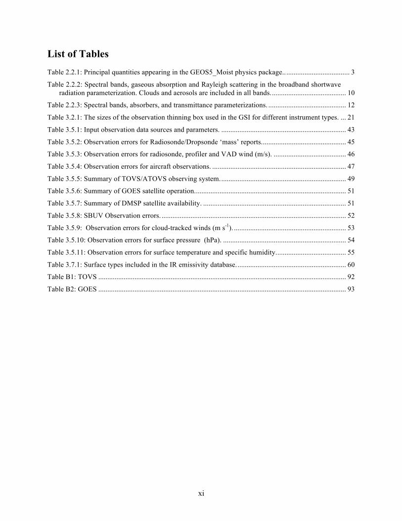
List of Tables Table 2.2.1: Principal quantities appearing in the GEOS5_Moist physics package.. ................................... 3 Table 2.2.2: Spectral bands, gaseous absorption and Rayleigh scattering in the broadband shortwave

radiation parameterization. Clouds and aerosols are included in all bands.......................................... 10 Table 2.2.3: Spectral bands, absorbers, and transmittance parameterizations. ........................................... 12 Table 3.2.1: The sizes of the observation thinning box used in the GSI for different instrument types. ... 21 Table 3.5.1: Input observation data sources and parameters. ..................................................................... 43 Table 3.5.2: Observation errors for Radiosonde/Dropsonde ‘mass’ reports............................................... 45 Table 3.5.3: Observation errors for radiosonde, profiler and VAD wind (m/s). ........................................ 46 Table 3.5.4: Observation errors for aircraft observations. .......................................................................... 47 Table 3.5.5: Summary of TOVS/ATOVS observing system...................................................................... 49 Table 3.5.6: Summary of GOES satellite operation.................................................................................... 51 Table 3.5.7: Summary of DMSP satellite availability. ............................................................................... 51 Table 3.5.8: SBUV Observation errors. ...................................................................................................... 52 Table 3.5.9: Observation errors for cloud-tracked winds (m s-1). .............................................................. 53 Table 3.5.10: Observation errors for surface pressure (hPa). .................................................................... 54 Table 3.5.11: Observation errors for surface temperature and specific humidity....................................... 55 Table 3.7.1: Surface types included in the IR emissivity database............................................................. 60 Table B1: TOVS ......................................................................................................................................... 92 Table B2: GOES ......................................................................................................................................... 93

xii

1

1. Introduction The assimilation system described in this document is a major new version of the Goddard Earth Observing System Data Assimilation System (GEOS DAS). The GEOS-5 DAS is based on the GEOS-5 Atmospheric General Circulation Model (AGCM) integrated with the Gridpoint Statistical Interpolation (GSI) Analysis. This represents a radical evolution of the GEOS system, with the adoption of the GSI analysis jointly developed with the National Centers for Environmental Prediction (NCEP) and a new set of physics packages for the AGCM. The first choice allows the Global Modeling and Assimilation Office (GMAO) to take advantage of the developments, especially that of radiance assimilation, at NCEP and the Joint Center for Satellite Data Assimilation (JCSDA), and facilitates our own contributions to the operational system. The second choice allows us to tune the system for both weather and climate applications, taking advantage of satellite observations in the assimilation context as we do so. The GEOS-5 AGCM maintains the finite-volume dynamics (Lin, 2004) used for GEOS-4 (e.g., Bloom et al., 2005) and found to be so effective especially for transport in the stratosphere (e.g., Pawson et al., 2007). This dynamical core is integrated with various physics packages (e.g., Bacmeister et al., 2006) under the Earth System Modeling Framework (ESMF) (e.g., Collins et al., 2005) including the Catchment Land Surface Model (CLSM) (e.g., Koster et al., 2000). The GSI analysis is a new three-dimensional variational (3DVar) analysis applied in grid-point space to facilitate the implementation of anisotropic, inhomogeneous covariances (e.g., Wu et al., 2002; Derber et al., 2003; Purser et al., 2003a, b). GMAO scientists have contributed to GSI development since 2004. During implementation in GEOS-5, this system has continued along its development path. One result of this was the need to address shocks introduced by imbalances in the mass-wind analysis increments. Although balance constraints are under development, in order to meet the GMAO’s production schedule requirements, the decision was made to re-introduce (from GEOS-3) the incremental analysis update (IAU) procedure (Bloom et al., 1996) and this has proven very effective. The primary performance drivers of the GEOS DAS products are temperature and moisture fields suitable for the EOS instrument teams, wind fields for the transport studies of the stratospheric and tropospheric chemistry communities, and climate-quality analyses to support studies of the hydrological cycle through the Modern Era Retrospective-analysis for Research Applications (MERRA, e.g., Bosilovich et al., 2006). Other significant drivers for the GEOS DAS have involved the provision of near real-time mission support for a number of atmospheric chemistry mission field campaigns. This report documents Version 0.1 of GEOS-5, also referred to as GEOS-5.0.1, the interim release used to meet the production timeline requirements of the EOS instrument teams. Upgrades implemented for Version 1.0, referred to as GEOS-5.1.0, address some of the deficiencies noted by the instrument teams and in our tuning of the DAS for MERRA. These are documented, as are those for Version 2.0, referred to as GEOS-5.2.0, which address some additional deficiencies noted by the CERES science team and some final model tuning and analysis upgrades for MERRA. This system documentation is organized as follows: The main characteristics of the atmospheric model are described in Chapter 2. The analysis system is described in Chapter 3. The assimilation system and observing system details are described in Chapter 4. The specific upgrades from GEOS-5.0.1 to GEOS-5.2.0 are documented in Chapter 5.

2

2. The GEOS-5 Atmospheric General Circulation Model The GEOS-5 atmospheric model is a weather-and-climate capable model being used for atmospheric analyses, weather forecasts, uncoupled and coupled climate simulations and predictions, and for coupled chemistry-climate simulations. Applications have used model configurations from 2° to 1/4° resolutions, with 72 layers to 0.01 hPa, resolving both the troposphere and the stratosphere. The AGCM relies heavily on ESMF, both superstructure and infrastructure, for its internal architecture (e.g., Collins et al., 2005). Parallelization is primarily implemented through MPI, although some key parts of the code, such as the model dynamics, also have Open-MP capability. The model runs on a 2-D decomposition, transposing internally between horizontal and vertical layouts. Some of the physics such as the solar radiation, which at any given time is active over only half the globe, is load balanced. The code scales well across compute nodes and scalability increases linearly with problem size. Developments of GEOS-5 were guided by a realistic representation of tracer transports and stratospheric dynamics. The ozone analysis of the DAS is input to the radiation package along with an aerosol climatology. GEOS-5 is coupled to a catchment-based hydrologic model (Koster et al., 2000) and a sophisticated multi-layer snow model (Stieglitz et al., 2001) that is coupled to the catchment hydrology.

2.1 Hydrodynamics The finite-volume dynamical core has an extensive documentation in the open literature (e.g., Lin, 2004, and references therein). The different implementation in GEOS-5 compared with GEOS-4 is merely a technical computational issue of layout on processing elements. GEOS-5 uses a 2-D horizontal decomposition.

2.2 Physics The physics package includes four major groups of physical processes: moist processes, radiation, turbulent mixing, and surface processes. Each of these in turn is subdivided into various components. The radiation module includes longwave and shortwave radiation submodules. The turbulent mixing consists of the vertical diffusion, planetary boundary layer parameterization, and gravity wave drag. The surface processes provide surface fluxes obtained from land, ocean and sea ice models.

2.2.1 Moist Physics Parameterizations In developing GEOS-5, attention has focused on the representation of moist processes. GEOS5_Moist considers liquid and ice phases of cloud condensate. Two separate cloud “types” are also recognized explicitly, with separate fraction and condensate variables kept for each type. The cloud types are distinguished by their source. One type, which will be denoted “anvil” cloud, originates in detraining convection. The second type, which is referred to as large-scale cloud, originates in a probability distribution function (PDF) based condensation calculation. Once created, condensate and fraction from the anvil and large-scale cloud types experience the same loss processes: evaporation, autoconversion, sedimentation and accretion. Parameter settings may vary by type, but identical formulations are used. Clouds associated with updraft cores are not treated prognostically, but rainfall from convective cores is disposed of within GEOS5_Moist.

3

Table 2.2.1: Principal quantities appearing in the GEOS5_Moist physics package. Quantities labeled “input/output” are AGCM prognostic fields that incur modifications due to moist processes. These fields are normally also modified by other model processes, e.g., advection. Those labeled “internal” are not modified by processes outside of GEOS5_Moist, and normally are not prognostic, that is, they are generated and disposed of within a single call to GEOS5_Moist. These fields are important in the internal dynamics of GEOS5_Moist but are normally not required by other model processes. Fields labeled “output” are products of GEOS5_Moist for other GEOS5 processes. These are used but may not be modified by other processes.

Variable Description Status u Zonal wind Input/output v Meridional wind Input/output T Air temperature Input/output q Specific humidity Input/output ql,ls Liquid cloud condensate large scale source (LS) Input/output qi,ls Frozen cloud condensate (LS) Input/output ql,an Liquid cloud condensate anvil source (AN) Input/output qi,an Frozen cloud condensate (AN) Input/output fls Cloud fraction (LS) Input/output fan Cloud fraction (AN) Input/output qp,l,ls Liquid precipitating condensate (LS) Internal qp,i,ls Frozen precipitating condensate (LS) Internal qp,l,an Liquid precipitating condensate (AN) Internal qp,i,an Frozen precipitating condensate (AN) Internal qc,cu Total (ice+liquid) cloud condensate in cumulus updrafts (CU) Internal qp,c,cu Total precipitating condensate (CU) Internal qp,l,cu Liquid precipitating condensate (CU) Internal qp,i,cu Frozen precipitating condensate (CU) Internal fcu Areal fraction of cumulus updrafts Internal φcu Mass flux in cumulus updrafts Internal Pcu Pan Pls

Surface flux of precipitation from cumulus updrafts Surface flux of precipitation from anvils Surface flux of precipitation from large scale clouds

Output Output Output

The basic sequence of events in GEOS5_Moist is as follows. First, the convective parameterization, Relaxed Arakawa-Schubert, or RAS (Moorthi and Suarez, 1992) is called. RAS estimates convective mass fluxes for a sequence of idealized convective plumes. Each plume produces detraining fluxes of mass and cloud condensate, as well as profiles of precipitating condensate. Adjustments to the environmental profiles of u, v, T and q are also calculated sequentially by each plume. Next, the large-scale cloud condensate scheme (PrognoCloud) is called. PrognoCloud first takes the detraining mass and condensate fluxes from RAS, if any exist, and adds them to the existing condensate and fraction of the anvil cloud type. Next, large-scale condensation is estimated using a simple assumed PDF of qtotal. This step produces a new fraction and condensate for the large-scale cloud type. Freezing of existing cloud condensate and partitioning of the new cloud condensate are also performed for both cloud types. After all sources of cloud condensate have been taken into account, four loss mechanisms are invoked: 1) evaporation of condensate and fraction, 2) autoconversion of liquid or mixed phase condensate, 3) sedimentation of frozen condensate, and 4) accretion of condensate by falling precipitation. Each of these losses is applied to both anvil and statistical cloud types. The formulation of these terms is detailed below.

4

In addition to producing and disposing of condensate, PrognoCloud handles the fallout of autoconverted (precipitating) condensate. Precipitating condensate is accumulated from the top down. In each model layer a typical drop size, fall speed, and residence time is estimated. These parameters are used to estimate re-evaporation of falling precipitation. The calculations are done separately for precipitation originating from each of the two cloud types, as well as for convective core precipitation. A profile of autoconverted condensate averaged over the grid-box within convective updrafts is one of the outputs of RAS. A schematic diagram of GEOS5_Moist is shown in Figure 2.2.1. Each process within GEOS5_Moist is discussed in greater detail below.

Figure 2.2.1: Schematic of Moist processes in GEOS-5. 2.2.1.1 Convection GEOS5_Moist uses a modified version of the scheme described by Moorthi and Suarez (1992). As in Moorthi and Suarez a sequence of linearly entraining plumes is considered with mass flux profiles given by

€

φk (z) =φ0k (1+ λkz) . The entrainment parameter for the k-th plume, λk, is determined by the choice of cloud base and cloud detrainment level. The GEOS-5 implementation is flexible in this respect. The default is to take an average of the two lowest model layers as the cloud-base layer. In GEOS-5 each model layer is tested, starting from the model level near 100 hPa and moving down to the level above cloud base. A random selection of plumes is also possible. However, this choice does not appear to have a major impact on model behavior as long as roughly similar numbers of plumes are invoked.

5

Once cloud base, detrainment level, and λk have been chosen, a series of calculations is made for the plume. A modified CAPE-based closure is used to determine the cloud base mass flux, φ0k. In addition to determining φ0k and λk a steady-state profile of vertical velocity, wk, is determined for each plume as first suggested by Sud and Walker (1999). The calculation of wk in GEOS-5 is simpler than that of Sud and Walker: the buoyancy force is vertically integrated from cloud base to detrainment level to obtain a velocity profile that is multiplied by an empirical tuning parameter:

€

wk =αw,cu g Tk −T0T0zB

zD∫ dz .

This approximate approach is employed because of the severe limitations inherent in the plume/parcel view of convection, including the neglect of pressure forces on the parcel. Autoconversion of convective condensate, qc,cu, to precipitating condensate, qp,c,cu, is also treated following Sud and Walker (1999). Once an updraft velocity profile wk(z) is estimated for each plume, it is used to derive time-scales Δzk/wk for parcels rising through the plume. These time-scales are then employed in simple temperature-dependent, Sundqvist-type expressions (Sundqvist, 1978) for autoconversion:

€

δqp,c,cu,k = −δqc,cu,k ≈C0,cu f (T ) 1 - exp−qc,cu,k

2

qc,crit2 / f (T )2

qc,cu,k

Δzkwk

.

Here, C0,cu is a base autoconversion rate for condensate in convective plumes. It is multiplied by a temperature dependent function f(T) specified below. The present model for the updraft velocity is much simpler than that employed by Sud and Walker: the buoyancy force is integrated in the vertical and scaled by a tunable parameter. Each plume modifies the environmental θ and q profiles. These modifications are felt by all subsequent plumes invoked during the call. In addition to the modification of the background thermodynamic state, the plumes detrain mass and condensate into the environment, so that net effects,

€

DM = Dkk∑ and DC = Dk qcc,k

k∑ ,

are obtained. DM and DC, the mass and condensate effects, respectively, are passed to PrognoCloud to serve as sources for anvil cloud fraction and anvil cloud condensate. A net profile of precipitating convective condensate,

€

PRAS = δqpc,kk∑ ,

is also passed to PrognoCloud. Finally, an estimate of updraft areal fractions is made using the total mass flux through each layer along with the local vertical velocity estimate.

2.2.1.2 Large-Scale Cloud Scheme Source Terms for Cloud. As described earlier, the scheme distinguishes two types of cloud, that produced by detraining convection and that produced by large-scale condensation. The first type will be referred to as anvil cloud here and denoted by the subscript an. The second type, statistical or large-scale clouds, will be denoted by the subscript ls. Anvil Cloud. Anvil cloud condensate, qc,an, and anvil cloud fraction, fan, are updated straightforwardly using DM and DC from RAS:

6

€

δfan = DM ρΔz and δqc,an = DC ρΔz .

Large-Scale Condensation. Condensation is based on a PDF of total water as in Smith (1990) or Rotstayn (1997). However, GEOS5_Moist uses a boxcar with a spread determined by the local saturation humidity, qsat. The current cloud scheme can be interpreted as a prognostic PDF scheme with a bi-modal structure as shown in Figure 2.2.2.

Figure 2.2.2: Schematic diagram of the implicit bi-modal PDF structure in the GEOS5_Moist cloud scheme. The current scheme consists of a boxcar PDF in non-anvil regions added to a δ-function containing contributions from detraining convection. In the symbols above, overbars refer to gridbox mean values. Freezing and Melting of Cloud Condensate Fresh (new) cloud condensate is partitioned initially according to temperature using,

€

fice(T ) =

0 T > TiceT −Tice

Tallice −Tice

4Tice > T > Tallice

1.0 T < Tallice

.

However, freezing progresses as long as the condensate remains in subfreezing temperatures. This freezing is parameterized as a temperature-dependent linear loss term for liquid condensate,

€

qtot =(1− fan )qtot,x* + fanqtot,an

*

qtot,an* =qsat (T)+qc,an

* ; qc,an= fanqc,an*

€

fanδ( ′ q − qtot,an* )

€

fkΔ

€

Δ = αqsat

7

€

q•

l,{ls,an}FRZ = −ql{ls,an}fice(T )τFRZ

.

Whenever T exceeds Tice melting of condensate is assumed to occur instantly and completely. A single ramped temperature-dependent saturation function is used for all calculations of saturation specific humidities. 2.2.1.3 Destruction of Cloud Destruction of cloud occurs in four ways: 1) evaporation “cloud munching”, 2) autoconversion of cloud condensate to precipitating condensate, 3) sedimentation of and 4) accretion of cloud condensate onto falling precipitation. Evaporation Cloud (Ec) “Munching” This mechanism is meant to represent destruction of cloud along edges in contact with cloud-free air. This process is parameterized using a microphysical expression from Del Genio et al. (1996), where U is an environmental relative humidity, qc is the cloud condensate mixing ratio, rc is the cloud droplet radius derived from an assumed number density, and A and B are temperature-dependent microphysical parameters. In GEOS-5 this loss is applied only to the anvil type. Autoconversion of Liquid and Mixed Phase Cloud (Ac) This is parameterized using the same Sundqvist-type formulation as used in the convective parameterization:

€

Ac{ls,an} =C0,{ls,an} f (T ) 1 - exp−ql,{ls,an}

2

qc,crit2 / f (T )2

ql,{ls,an} .

Figure 2.2.3: “Sundqvist-factor” controlling low-temperature autoconversion.

The same temperature-dependent factor f(T) is used for ls and an clouds. The behavior of f (T) is shown in Figure 2.2.3. The increase below 273K represents accelerated production of precipitation in mixed-

€

Ec = −CE, c1−U

ρw (A+B)rc2 qc ,

8

phase clouds. The choice of this function is largely empirical. Destruction of cloud fraction by autoconversion is not considered. Rapid conversion or fallout of frozen ice crystals is handled explicitly using the sedimentation formulation described next. Sedimentation of Ice Cloud (Sc) This is parameterized using cirrus ice fall speeds given by Lawrence and Crutzen (1998). However, instead using their regime division based on latitude, their expression for tropical cirrus is assigned to anvil clouds, and their mid-latitude form is assigned to large-scale clouds:

€

WF ,i,an =128.6+53.2log10(qc,i,an )+5.5[log10(qc,i,an )]2

WF ,i, ls =106 (qc,i, ls)0.16 .

A simple one-way advection is used to represent the transition of ice cloud particles to sedimenting particles - the “fall through” approximation (e.g., Le Treut et al., 1994):

€

Sc = −CS{ls,an} qi,{ls, an}WF ,i{ls,an}

Δz

with empirically tuned parameters CS{ls,an}. This approximation is known to overestimate production of frozen precipitation in other models (Rotstayn, 1997). Fallout and Re-evaporation of Precipitation and Accretion of Cloud Condensate All precipitation, including that produced within convective plumes, is finally disposed of in PrognoCloud. Three streams of precipitation, each with two phases, are considered: liquid and frozen precipitating condensate from ls clouds - qp,i,ls and qp,l,ls; liquid and frozen precipitating condensate from an clouds - qp,i,an and qp,l,an, and liquid and frozen precipitating condensate from convective plumes (cu) - qp,i,cu and qp,l,cu. The inputs to the subroutine are mixing ratios of precipitating condensate. The precipitating condensate in each stream and phase is accumulated from the top assuming complete fallout to obtain the downward flux of precipitation at level k, P↓

box (k). To account for subgridscale variability in precipitation this flux is scaled by a “shower area factor”, As defined below, P↓S = P↓box − AX

-1. This scaled flux is then used to estimate a typical drop size rp using the Marshall-Palmer distribution. The quantity rp is used to estimate precipitation fall velocities WF,p and ventilation factors Ve for the precipitation. These are now used along with the vertical thickness of layer k to estimate the fractional re-evaporation of precipitating condensate during its passage through the layer. The shower area factor As is calculated slightly differently for convective and non-convective precipitation. For convective precipitation a weighted vertical mean of the updraft areal fraction is used. For non-convective precipitation, qp,an and qp,ls, a similar weighted mean is calculated using the corresponding cloud fraction in place of updraft area fraction. The parameter Ef, the “exposed fraction”, represents the fraction of precipitation exposed to grid-box mean values of relative humidity, as opposed to the shielded fraction Sf = 1-Ef which falls through a saturated cloudy environment (Figure 2.2.4). For non-convective precipitation we assume Ef=1. For convective precipitation a shear-dependent exposure is assumed.

9

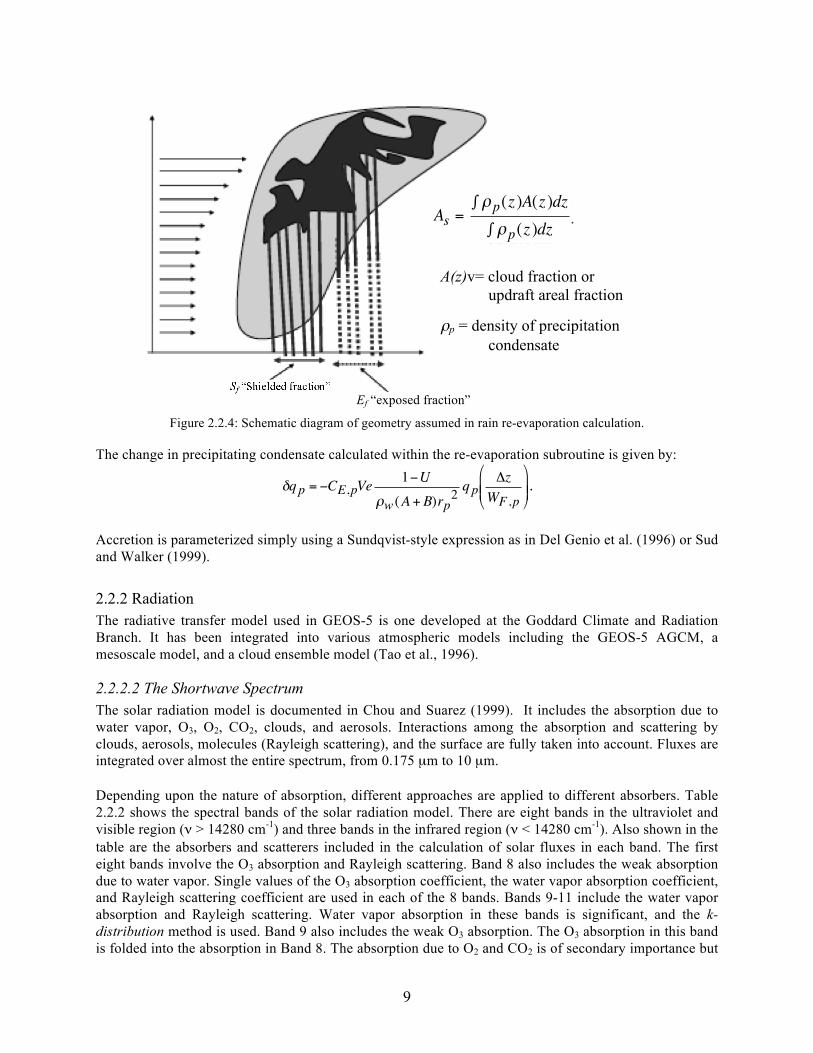
Figure 2.2.4: Schematic diagram of geometry assumed in rain re-evaporation calculation.

The change in precipitating condensate calculated within the re-evaporation subroutine is given by:

€

δqp = −CE,pVe1−U

ρw (A+B)rp2 qp

ΔzWF ,p

.

Accretion is parameterized simply using a Sundqvist-style expression as in Del Genio et al. (1996) or Sud and Walker (1999).

2.2.2 Radiation The radiative transfer model used in GEOS-5 is one developed at the Goddard Climate and Radiation Branch. It has been integrated into various atmospheric models including the GEOS-5 AGCM, a mesoscale model, and a cloud ensemble model (Tao et al., 1996). 2.2.2.2 The Shortwave Spectrum The solar radiation model is documented in Chou and Suarez (1999). It includes the absorption due to water vapor, O3, O2, CO2, clouds, and aerosols. Interactions among the absorption and scattering by clouds, aerosols, molecules (Rayleigh scattering), and the surface are fully taken into account. Fluxes are integrated over almost the entire spectrum, from 0.175 µm to 10 µm. Depending upon the nature of absorption, different approaches are applied to different absorbers. Table 2.2.2 shows the spectral bands of the solar radiation model. There are eight bands in the ultraviolet and visible region (ν > 14280 cm-1) and three bands in the infrared region (ν < 14280 cm-1). Also shown in the table are the absorbers and scatterers included in the calculation of solar fluxes in each band. The first eight bands involve the O3 absorption and Rayleigh scattering. Band 8 also includes the weak absorption due to water vapor. Single values of the O3 absorption coefficient, the water vapor absorption coefficient, and Rayleigh scattering coefficient are used in each of the 8 bands. Bands 9-11 include the water vapor absorption and Rayleigh scattering. Water vapor absorption in these bands is significant, and the k-distribution method is used. Band 9 also includes the weak O3 absorption. The O3 absorption in this band is folded into the absorption in Band 8. The absorption due to O2 and CO2 is of secondary importance but

€

As =ρp(z )A(z )dz∫

ρp(z )dz∫

A(z)v= cloud fraction or updraft areal fraction ρp = density of precipitation condensate

Ef “exposed fraction”

10

occurs in wide spectral ranges. Different approaches which compute only the reduction in fluxes are used. Clouds and aerosols are included in all bands.

Table 2.2.2: Spectral bands, gaseous absorption and Rayleigh scattering in the broadband shortwave radiation parameterization. Clouds and aerosols are included in all bands.

Spectral Range Band

(cm-1) µm Absorber/Scatterer

1 44440-57140 0.175-0.225 O3 Rayleigh

2 40820-44440 35700-38460

0.225-0.245 0.260-0.280

O3 Rayleigh

3 38460-40820 0.245-0.260 O3 Rayleigh

4 33900-35700 0.280-0.295 O3 Rayleigh

5 32260-33900 0.295-0.310 O3 Rayleigh

6 31250-32260 0.310-0.320 O3 Rayleigh

7 25000-31250 0.320-0.400 O3 Rayleigh

8 14280-25000 0.400-0.700 O3, H2O Rayleigh

9 8200-14280 0.70-1.22 H2O O3* Rayleigh

10 4400-8200 1.22-2.27 H2O Rayleigh

11 1000-4400 2.27-10.0 H2O

Total Spectrum O2 CO2

* O3 absorption is folded into Band 8. Reflection and transmission of a cloud and aerosol-laden layer are computed using the δ-Eddington approximation. Fluxes are then computed using the two-stream adding approximation. For a cloud layer, the optical thickness is parameterized as a function of cloud water/ice amount and the effective particle size, whereas the single-scattering albedo and asymmetry factor are parameterized as a function of the effective particle size. Parameterizations are applied separately to water and ice particles. A maximum-random approximation, a combination of maximum and random cloud overlapping schemes, is adopted for the overlapping of clouds at different heights. Aerosol optical properties are specified input parameters, as is the surface albedo which is specified separately for the UV and PAR region and the infrared. It is also separately specified for direct and diffuse fluxes. Hence, a set of four surface albedos must be specified as input to the radiation routine. A special feature of this model is that absorption due to a number of minor absorption bands is included. Individually the absorption in those minor bands is small, but collectively the effect is large, about 10%

11

of the atmospheric heating. Integrated over all spectral bands and all absorbers, the surface heating is computed accurately to within a few watts per meter squared of high spectral-resolution calculations, and the atmospheric heating rate between 0.01 hPa and the surface is accurate to within 5%. 2.2.2.2 The Thermal Infrared Spectrum The longwave radiation model is documented in Chou et al. (2001). The parameterization includes the absorption due to major gaseous absorption (water vapor, CO2, O3) and most of the minor trace gases (N2O, CH4, CFC's), as well as clouds and aerosols with optical properties specified as input parameters. The thermal infrared spectrum is divided into nine bands and a sub-band. Table 2.2.3 shows the spectral ranges for these 10 bands, together with the absorbers involved in each band. The water vapor line absorption covers the entire IR spectrum, while the water vapor continuum absorption is included in the 540-1380 cm-1 spectral region. The absorption due to CO2 is included in the 540-800 cm-1 region, and the absorption due to O3 is included in the 980-1100 cm-1 region. The minor absorption due to CH4, N2O, CFC's, and CO2 is scattered between 800 cm-1 and 1380 cm-1 region in Bands 4-7. The absorption due to N2O in the 17µm region is included in sub-band 3a and is identified as Band 10. Chou et al. (2001) approximates the band-integrated downward and upward longwave fluxes as:

€

Fi↓( p) = Bi0

p∫ ( ′ θ ) ∂Ti ( p, ′ p )∂ ′ p

d ′ p ,

€

Fi↑( p) =εiBi (θs)Ti ( p, ps) + Bi0

p∫ ( ′ θ ) ∂Ti ( p, ′ p )∂ ′ p

d ′ p + (1−εi)Fi↓( ps)Ti ( p, ps),

where

€

Ti ( p, ′ p ) ≈ 1Bi (θ0)

BνΔν i∫ (θ0)Tν ( p, ′ p )dν ,

€

Bν (θ) is the Planck flux,

€

Tν ( p, ′ p ) is the flux transmittance for isotropic radiation,

€

Bi (θ) = Bν (θ)Δν i∫ ,

€

εi is the surface emissivity,

€

ps is the surface pressure,

€

θs is the Earth’s surface skin temperature, and

€

θ0 is a typical value of the atmospheric temperature, set to 250K. The spectrally integrated Planck fluxes were pre-computed for each band and then fit with a fifth-degree polynomial in temperature. When integrated over all bands, errors in this regression are negligible (< 0.1%) for 150K < θ< 350K. The regression coefficients are given in Chou et al. (2001). The polynomial approximation is used to calculate sensitivity of the upward fluxes to the surface temperature. Since the longwave radiation parameterization is called less often than the boundary layer and land surface parameterizations, all fluxes are linearized about the surface temperature at the beginning of the radiation interval, and radiative heating rates are recomputed based on this linearization at each time step. To achieve a high degree of accuracy and speed, various approaches of computing the transmission function are applied to different spectral bands and gases. The gaseous transmission function is computed either using the k-distribution method or the table look-up method. Table 2.2.3 shows the bands, the absorbers, and the method used to compute transmission in each band. To include the effect of scattering due to clouds and aerosols, the optical thickness is scaled by the single-scattering albedo and asymmetry factor. The optical thickness, the single-scattering albedo, and the asymmetry factor of clouds are parameterized as functions of the ice and water content and the particle size. The aerosol amounts are specified input parameters together with a function that computes optical

12

thickness, single-scattering albedo, and asymmetry factor for each aerosol and each of the 10 bands at every atmospheric layer. The aerosols used in GEOS-5 correspond to the 15 species of dust, carbon, sulfate, and sea-salt currently used in the Goddard Chemistry Aerosol, Radiation, and Transport (GOCART) aerosol model (Chin et al., 2002). These can be produced by the GOCART model or read in as specified 4-dimensional distributions. The parameterization can accurately compute fluxes to within 1% of the high spectral-resolution line-by-line calculations. The cooling rate can be accurately computed in the region extending from the surface to the 0.01-hPa level.

Table 2.2.3: Spectral bands, absorbers, and transmittance parameterizations.

Band Spectral Range (cm-1) Absorber

Transmittance Parameterization

Method 1 0-340 H2O line T 2 340-540 H2O line T 3a 540-620 3b 620-720 3c 720-800

H2O, CO2 line H2O continuum

T C

4 800-980 H2O line H2O continuum CO2, F11, F12, F22

K C K

5 980-1100 H2O line, CO2, F11 H2O continuum O3

K C T

6 1100-1215 H2O line H2O continuum H2O, CH4, F12, F22

K C K

7 1215-1380 H2O line, N2O, CH4 H2O continuum

K C

8 1380-1900 H2O line T 9 1900-3000 H2O line H

10 540-620 H2O line, CO2, N2O H2O continuum

K C

K: k-distribution method with linear pressure scaling. T: Table look-up with temperature and pressure scaling. C: One-parameter temperature scaling for water vapor continuum absorption. In GEOS-5 cloud properties and amounts are predicted at each model layer. In the radiation code, the layer clouds are grouped into three height ranges: high, middle and low, separated approximately by 400 hPa and 700 hPa pressure levels. Clouds in layers within each height group are assumed maximally overlapped, and clouds among the three height groups are assumed randomly overlapped. Different types of aerosols are allowed to co-exist in a layer. The total effective optical thickness, single-scattering albedo, and asymmetry factor of a layer are computed similarly to those of clouds.

2.2.3 Turbulent Mixing The free atmospheric turbulent diffusivities are based on the gradient Richardson number. Two atmospheric boundary-layer turbulent mixing schemes are used. The Louis et al. (1982) scheme is used in stable situations with no or weakly-cooling planetary boundary layer (PBL) cloud. The Lock et al. (2000) scheme is used for unstable or cloud-topped PBLs. The latter scheme includes a representation

13

of non-local mixing (driven by both surface fluxes and cloud-top processes) in unstable layers, either coupled to or decoupled from the surface, and an explicit entrainment parameterization. The scheme is formulated in the moist conserved variables θl, the liquid–frozen water potential temperature, and qt, the specific total water content, so that it can treat both dry and cloudy layers. In GEOS-5, the scheme is extended so that unstable surface parcel calculations include moist heating and entrainment. GEOS-5 incorporates two gravity wave drag parameterizations, an orographic gravity wave drag formulation based on McFarlane (1987), and a formulation for non-orographic waves based on Garcia and Boville (1994). The mountain waves are forced by the sub-grid orographic variability, h' = sqrt ( avg( [ h- avg(h) ]2) ), where avg() denotes an average over the scale of gridbox. The terrain data, h(x,y), is from the GTOPO30 data (http://edc.usgs.gov/products/elevation/gtopo30/gtopo30.html), with approximately 1 km resolution. The smallest scales (< 10km) are not used to force gravity waves, but enter into an orographic form drag used in the turbulence. The nominal gravity amplitude at the surface is given by MIN(h', U/N), where U is the surface wind speed and N is the low level stratification frequency. The non-orographic waves, important in the stratosphere and mesosphere, are launched at 100 hPa. GEOS-5 uses an 8 wave-spectrum, with waves at phase speeds of 10, 20, 30 and 40 ms-1 in both directions with respect to the wind at launch level. Their amplitude depends on their phase speed in a Gaussian way, ~ exp( ( -c / 30)2 ). The amplitude is modified according to latitude, ranging from full amplitude in both polar regions (90-45 latitude bands) and dropping to 0.2 of the base amplitude in the tropics (20°S-20°N). The base amplitude, i.e., a wave with c approaching 0 near the poles, is 6.4e-3 N m-2.

2.2.4 Chemical Species 2.2.4.1 The Ozone Model Rather than transporting ozone (O3), the GEOS-5 model transports the odd-oxygen family:

Ox = O3 + O(3P) + O(1D). The chemical change in Ox is computed by

Ox(t + dt) = (Ox* + P dt ) / ( 1 + L dt ), where t is time, P is the Ox production rate, L is the Ox loss frequency, and Ox* is the intermediate Ox field that includes effects of transport and turbulent processes. Zonally-invariant and monthly-averaged coefficients P and L are used, as generated by the Goddard two-dimensional chemistry and transport model with surface source gas boundary conditions for the year 2000 (Fleming et al., 2001). Ozone is derived from Ox. O3 is specified to be equal to Ox for pressure higher than 1 hPa. At pressures lower than 1 hPa, O3 is specified as equal to Ox during the nighttime and as

O3 = Ox exp[-1.5(log10 p)2], in the daytime, where p is pressure in hPa. This relation is an empirical fit to equatorial daytime O3/Ox ratios in a simulation that utilized a complete stratosphere-mesosphere chemistry mechanism. The diurnal ozone variation is due to fast ozone photolysis and subsequent recombination during nighttime in the mesosphere. To avoid development of a low ozone bias in the upper stratosphere in GEOS-5, Ox production rates are adjusted following Stajner et al. (2004). The Ox production rates are modified so that the ozone chemical

14

balance (which is P/L in the stratosphere) agrees with ozone climatologies from the Upper Atmosphere Research Satellite data (http://hyperion.gsfc.nasa.gov/Public/Analysis/UARS/urap/home.html) and SBUV data (Langematz, 2000). 2.2.4.2 Other Constituents The other radiatively active species, methane (CH4), nitrous oxide (N2O), chlorofluorocarbons (CFC-11, CFC-12), hydrochlorofluorocarbon (HCFC-22), and stratospheric water vapor (H2O) are specified from the steady-state climatology of the Goddard two-dimensional chemistry and transport model, which employed surface source gas boundary conditions from 2000.

2.2.5 Surface Processes The surface exchange of heat, moisture and momentum between the atmosphere and land, ocean or sea ice surfaces are treated with a bulk exchange formulation based on Monin-Obukhov similarity theory. GEOS-5 employs specified distributions of sea surface temperatures and sea ice, either from an observed weekly/monthly mean time series or annually repeating climatological mean. The sea ice distribution is prescribed.

2.2.6 The Catchment Land Surface Model GEOS-5 is coupled to a catchment-based hydrologic model (Koster et al., 2000) and a sophisticated multi-layer snow model (Stieglitz et al., 2001). 2.2.6.1 Overview The one-dimensional "layered" framework used by traditional land surface models (LSMs) is arguably not amenable to an adequate treatment of runoff generation or subsurface soil moisture movement, since both processes in nature are largely controlled by spatial heterogeneity in soil moisture. The development of the GMAO Catchment LSM (Koster et al., 2000, Ducharne et al., 2000) is an attempt to improve treatment of the subgrid horizontal structure of land surface hydrological processes. In this LSM, subgrid heterogeneity in surface moisture state is treated statistically, since computational constraints (now and in the foreseeable future) prevent its explicit resolution. Nevertheless, the applied distributions are related sensibly to the topography, which exerts a major control over much of the subgrid variability. 2.2.6.2 Modeling Approach The approach is illustrated in Figure 2.2.5, which shows three different levels of the (shallow) water table and the associated partitioning of the surface into three regions: (1) a saturated region, from which evaporation occurs with no water stress and over which rainfall is immediately converted to surface runoff, (2) a subsaturated region, from which transpiration occurs with limited water stress and over which rainwater infiltrates the soil, and (3) a “wilting” region, in which the water stress shuts down the transpiration completely. The relative areas of these regions, which vary in time, are unique functions of the local topography and the values of the Catchment LSM's three water prognostic variables. By continually partitioning the catchment into hydrologically distinct regimes and then applying different runoff and evaporation physics in the different regimes, the Catchment LSM should, at least in principle, produce a more realistic simulation of areally-averaged surface energy and water processes.

15

Figure 2.2.5: Separation of the catchment area into hydrological regimes.

The soil water prognostic variables used by the Catchment LSM are “non-traditional” in that they are not strictly associated with soil layers. The main variable, the “catchment deficit”, describes the equilibrium water table distribution and the associated distribution of the equilibrium soil moisture profiles in the overlying vadose zone. The second variable describes the degree to which the root zone is out of equilibrium with the catchment deficit, and the third describes the degree to which the near-surface moisture is out of equilibrium with the other two variables. The water transfer between the three variables and the baseflow flux out of the system are controlled in part by the local topography. The model's other prognostic variables include an interception reservoir water content, a surface temperature, and the heat contents of six subsurface soil layers, from which time-varying vertical profiles of soil temperature over several meters can be derived. The model allows explicit vegetation control over the computed surface energy and water balances, with environmental stresses (high temperatures, dry soil, etc.) acting to increase canopy resistance and thus decrease transpiration. Six fundamentally different types of vegetation are considered in the current version of the Catchment LSM: broadleaf evergreen trees, broadleaf deciduous trees, needleleaf trees, grassland, shrubs, and tundra vegetation. Bare soil evaporation, transpiration, and interception loss occur in parallel. The energy balance formulations in the model (again, applied separately in each hydrological regime) were derived in large part from the Mosaic land surface model (Koster and Suarez, 1996), which in turn borrowed heavily from the SiB model of Sellers et al. (1986) for the transpiration calculation. Snow is modeled using three prognostic variables (heat content, snow water equivalent, and snow depth) in each of three layers (Stieglitz et al., 2001). The melting and refreezing of snow, snow compaction, liquid water retention, and the impact of snow density on thermal conductivity and albedo are explicitly treated.

M1

M2 M3

Saturated fraction equals zero; part of catchment now below wilting point.

Lower water table leads to smaller saturated fraction

Significant saturated fraction leads to high surface runoff

PLAN VIEW: M1 PLAN VIEW: M2 PLAN VIEW: M3

ground surface water table height

16

2.2.6.3 Implementation in GEOS-5 The Catchment LSM's implementation into the GEOS-5 system involves the “tiling” of a surface grid cell into a number of independent and irregularly shaped hydrological “catchment” elements. The catchment boundaries are derived from a 30-arc-second resolution (approximately 1 km) digital elevation model (DEM) provided by the U.S. Geological Survey. The delineation procedure considers network topology and drainage area (Verdin and Jenson, 1996; Verdin and Verdin, 1999) along with the application of ordering rules associated with a catchment coding system. For computational efficiency, and to take advantage of resolved heterogeneity in atmospheric forcing, catchments that straddle adjacent grid cells are separated into independent adjoining catchments, one in each grid cell. Runoffs produced by these artificially separated catchments can be combined into a single runoff that can then be routed across the continent. Global distributions are needed for a number of model parameters. The global HYDRO1K data set produced by the U.S. Geological Survey provided the distributions of compound topographic index needed to compute, within each catchment element, the parameters that control the shape of the shallow water table (using a TOPMODEL-type construct). Global soil texture information is derived from a 5-minute data set assembled by Reynolds et al. (1999). Global seasonal climatologies of leaf area index and greenness fraction are taken from AVHRR-based data generated at the University of Wales and compiled by the Global Soil Wetness Project (Dirmeyer et al., 2006). Global distributions of vegetation type are taken from http://edcsns17.cr.usgs.gov/glcc/globdoc2_0.html, the Earth Resources Observation and Science website. GEOS-5 uses a two-stream approximation that lets snow-free albedo (for the visible and near-infrared bands) vary with solar incidence angle, but the values so produced are scaled so that they are consistent, on the monthly time scale, with the snow-free albedos produced by Moody et al. (2005) from MODIS data. Global surface emissivity data are taken from Wilbur et al. (1999). 2.2.6.4 Testing of the Catchment LSM Various incarnations of the Catchment LSM have been evaluated extensively against observations through participation in the PILPS-2e project (Bowling et al., 2003), the Rhone-AGG project (Boone et al., 2006), and the second phase of the Global Soil Wetness Project (Dirmeyer et al., 2006). In addition, the Catchment LSM has proven to be an effective host for a soil moisture data assimilation system (Reichle and Koster, 2005; Reichle et al., 2007).

2.3 Specific Implementation for GEOS-5.0.1, GEOS-5.1.0, and GEOS-5.2.0. The GCM used in GEOS-5.0.1 has a 0.5° latitude by 0.625° longitude horizontal resolution, with the prognostic variables discretized on a staggered D-grid (Figure 2.3.1). There are 72 vertical layers from the surface to 0.01 hPa. This system has an effective time step of 30 minutes, which is the time step of its physics parameterization (although the dynamics time step is considerably shorter). The primary variables are: wind components (u,v); scaled virtual potential temperature (θ*=Tv/pκ); pressure thickness (of the Lagrangian control volume, p); and specific humidity (q).

17

Figure 2.3.1: Lagrangian control volume and state variables for the GEOS-5 AGCM.

2.3.1 Ancillary Initial and Boundary Data A climatological aerosol distribution is used (Colarco et al., 2008). The model uses either a climatological ozone distribution or (in DAS mode) the ozone analysis generated from the DAS. The surface orography and its sub-grid scale standard deviation were derived from the 30-second US Geological Survey Global Topographic Data (GTOPO30). An area-preserving algorithm is used to map the high-resolution GTOPO30 data set to model resolutions. The sea surface temperature and sea ice concentrations are derived from the weekly 1° Reynolds sea surface temperature (ERSST) version 2 (Reynolds et al., 2002). They are updated every time step using linear interpolation in time. GEOS-5 also employs an option to nudge the stratospheric water vapor to the zonal mean climatological HALOE (Halogen Occultation Experiment) (Randel et al., 1998) and MLS (Microwave Limb Sounder) water vapor data.

2.3.2 The Model Grid The GEOS-5 terrain-following Lagrangian control volume (lcv) coordinates are similar to an eta coordinate system. The model output and many of the GEOS-5.0.1 products are lcv products. The products include the full three-dimensional pressure variables at both layer centers (PLijl) and layer edges (PLEijl). The pressures reported are on a hybrid-sigma coordinate. Indexing in the vertical starts at the top, i.e., lcv layer 1 is the layer at the top of the atmosphere; lcv layer 72 is adjacent to the earth’s surface.

18

3. The GEOS-5 Analysis At the heart of the DAS is the analysis itself. The analysis combines information from irregularly distributed observations with a model state in such a way as to minimize a specified cost function. The model state (the background used for the analysis first guess) is obtained from a forecast initialized from a previous analysis. The weights assigned to each contribution to this combination depend on the specified error (or uncertainty) statistics for each of the observations and the model background. The GEOS-5 DAS uses the GSI analysis solver developed at NCEP. Other essential components are the quality-control software and the Radiative Transfer Model (RTM) needed for the radiance assimilation. The GSI is coupled to the Community Radiative Transfer Model (CRTM) developed through the JCSDA. For the stratospheric sounding unit (SSU) data used in MERRA, the GSI has been coupled to the GLATOVS RTM. Some details of the GSI are presented in Section 3.1. The background (model forecast) error statistics are discussed in Section 3.2. The observation streams and their error characteristics are presented in Section 3.3. The RTMs are presented in Section 3.4. Information pertaining to the implementation of the analysis for versions 5.0.1 and 5.1.0/5.2.0 of GEOS-5 is given in section 3.2.5.

3.1 The GSI Solver The GSI solver was developed at NCEP to support their unified 3D-Var analysis system for global and regional models. The GSI builds upon the Spectral Statistical Interpolation (SSI) analysis which is documented at http://www.emc.ncep.noaa.gov/gmb/gdas/. The analysis variables are defined in grid space and recursive filters are the basic building blocks used to create background error covariance structures (Derber et al., 2003). The implementation uses the recursive filters to produce approximately Gaussian smoothing kernels and isotropic correlation functions (Wu et al., 2002). By superposition of Gaussian kernels with different length scales it is possible to generate non-Gaussian shapes, and generally to implement a large class of flow-dependent inhomogeneous background error covariance models (Purser et al., 2003a,b). The variational analysis, xa, is obtained by minimizing the scalar cost function

€

J(x) = (x − xb)T B−1(x − xb) + [y − h(x)] T [E +F]−1 [y − h(x)] + JC

with respect to the control vector, x. The background, xb, represents a prior estimate of x and B is its expected error covariance. The vector y contains the available observations, the operator (also called the forward model) h(x) simulates these observations from x, and E+F=R contains the expected observation error covariances, including both instrument and representativeness errors. JC represents additional constraints that can be imposed, such as mass-wind balance and moisture constraints. The control vector or set of analysis variables, x, represents the atmospheric state at the central point in a 6-hour time window as well as predictor coefficients used for radiance bias correction (Derber and Wu, 1998; Dee, 2004, 2005) and surface temperatures used to correct model deficiencies at radiance data locations (Simmons, 2000). The forward model h(x) transforms the model variables into pseudo-observations. The pseudo-observation value at the observation time is obtained by linear interpolation using background states provided at the analysis time and 3 hours before or after the analysis time. The forward model can be as simple as interpolation from model grid point to the observation location, or as complex as a radiative transfer model for satellite observations.

19

To accommodate nonlinear operators h (e.g., precipitation, wind speed, penalties on q for supersaturation and negative values), J(x) is minimized using an incremental strategy (Courtier et al., 1994) in which the problem is repeatedly linearized about an updated current solution (the outer loop). In the first outer loop iteration, the current solution is the 6-hour forecast. In later iterations, the current solution is the result from the previous iteration. Currently, only two outer loops are performed due to computational considerations. A pre-conditioned conjugate gradient algorithm (the inner loop) is used to minimize the resulting quadratic cost function for the increments. The conjugate gradient algorithm requires the gradient of J with respect to the analysis variables. The gradient is evaluated using the adjoint of the transformation of the analysis variables into the observation variables. The control variables, x, are:

ψ: stream function contribution to wind χunbal: unbalanced velocity potential function Tunbal: unbalanced temperature Punbal: unbalanced surface pressure q: moisture cw: cloud water O3: ozone

and coefficients for the bias correction of the satellite radiance data. The balanced part of the temperature is defined by Tbal = Gψ, where G is an empirical matrix that projects increments of stream function at one level to a vertical profile of the balanced part of the temperature increments. G is latitude dependent. The balanced part of the velocity potential is defined as χbal = c ψ, where the coefficient c is function of latitude and height. The explained variance for balanced temperature and velocity potential as a function of height at 60°N is shown in Figure 3.1.1. The balanced part of the surface pressure increment is defined as Pbal = Wψ, where the vector W integrates the appropriate contribution of the stream function from each level. The explained variance of the balanced surface pressure calculated in this manner is shown as a function of latitude in Figure 3.1.2. Figure 3.1.1: The explained variance of the balanced part of temperature (red curve) and velocity potential (green curve) at 60°N used in GEOS-5.0.1 (left) and GEOS-5.1.0 (right). The balanced velocity potential is largest at the surface to include a surface friction effect.

20

Figure 3.1.2: The explained variance of the balanced surface pressure as a function of latitude.

The updated (analyzed) fields are: zonal and meridional wind components (u,v), temperature (T), moisture (q), cloud water (cw), ozone (O3), surface pressure (ps), surface temperature (Tskin). The analyzed wind components are calculated from the stream function and velocity potential.

3.2 The Treatment of Satellite Radiance Data Satellite data have become an essential part of the observing system. They represent by far the largest volume of data ingested into operational NWP assimilation systems and their use in these systems has a measurable positive impact on forecast skill scores, especially in the Southern Hemisphere. The analysis procedures for satellite radiance data are presented in Derber and Wu (1998) and McNally et al. (2000). As input to the surface emissivity calculation and the radiative transfer calculation of h(x), the background profiles of temperature, moisture (mixing ratio) and ozone (mixing ratio), and the surface temperature and 10-m wind speed are interpolated to the observation location and the pressure levels used by the radiative transfer scheme. Based on this information and the surface type, the radiative transfer code generates a pseudo-observation of brightness temperature and the Jacobian matrix needed for the minimization.

3.2.1 Data Thinning The large volume of satellite data and the expense of including them in analyses forces a subsetting or thinning of these observations prior to assimilation. In addition, the errors implied by the combined observation and radiative-transfer error covariance matrix should be correlated both between adjacent observations and between channels of the same sounding. In practice, it is difficult to estimate these correlations; therefore, the observation errors are assumed to be un-correlated and this matrix is diagonal. In the GSI, the thinning strategy is defined by a specified resolution for each instrument type, the likelihood of the observation passing a quality control (QC) window check, the underlying surface properties, the difference between the observation time and the analysis time, and the distance between the observation location and the center of the analysis grid box. The size of the thinning box for each instrument type is summarized in Table 3.2.1.

21

Table 3.2.1: The sizes of the observation thinning box used in the GSI for different instrument types.

Instrument

Type AMSU-A AMSU-B/MHS HIRS/AIRS

GOES Sounder/Imager SSM/I SSU

Thinning Box Size 145 km 240 km 180 km 160 km 200 km

3.2.2 Satellite Data Bias Correction Substantial biases are evident when satellite data are compared to the pseudo-observations derived from the background model [e.g., Eyre et al., 1993]. These biases may be due to bias in the background fields, or to errors in ground processing or in the forward processing (e.g., radiative transfer), residual contamination of the observations from cloud, instrument calibration errors, or inaccurate specification of instrument spectral response filters. Derber and Wu (1998) ascribe the dominant sources of these biases to ground processing errors and uncertainties in the radiative transfer calculation. The biases vary spatially and depend on other satellite parameters such as the local zenith angle. For many channels, the mean value of the bias (calculated as the difference between the observed radiance (O) and that (F) calculated from the model background) is large relative to the instrument noise. It is therefore necessary to apply corrections either before the radiances are used in the assimilation or during the assimilation procedure. The latter approach, termed adaptive bias correction, has the advantage that the system automatically adjusts the bias estimate for the satellite data so as to maintain consistency with all available information, i.e., both the model background and all other observations. One of the disadvantages of this method is the possibility that the model bias will become incorporated in the coefficients and feed back into the system and amplify the model bias. Dee (2005) describes the bias estimation procedure as follows. Bias parameters are estimated along with the model state in a variational analysis by augmenting the control vector with those bias parameters. To be explicit, the cost function of Section 3.1 can be written as

€

J(x) = (x − xb)T B−1(x − xb) + (b−bb )

T Bβ−1(b−bb )+ [y − h(x)− b(x,b)] T R−1 [y − h(x)− b(x,b)] + JC .

The errors in the background estimate for the predictor coefficients, βb, are generally correlated with the errors in the state estimate because they depend on the same data, however, because of lack of information, the cross-covariance in the GSI implementation is assumed to be zero giving the form of the cost function above. The implementation in the GSI relies on linear predictor models so that the bias model included in the forward model is

€

b(x,b) = βi pi (x)i=0

N p∑ ,

where b is the bias model and the pi are the predictors. Only a few predictors are used in order not to over-fit the biases, but the predictor coefficients for each channel and each sensor are allowed to be different. In the GSI, p0 is a constant and the other predictors are: scan angle, lapse rate, lapse rate squared and (for microwave instruments) cloud liquid water. The predictors are scaled so that the same background error variance is used for each coefficient. A bias estimate is made for each scan position (for GOES it is for each integer local zenith angle). The total number of radiance bias parameters included in the system is roughly N = Np ×Ns × Nc, where Np is the number of predictors used, Ns is the number of sensors being assimilated, and Nc is the number of channels per sensor.

22

(a) (b)

The background estimate for β is the estimate obtained from the previous analysis. The bias estimates spin up to a stable estimate fairly quickly, viz., a few days. In GEOS-5, new satellite data are only introduced after a two-week passive assimilation used to estimate the bias parameters. Figure 3.2.1a gives an example of the observation minus forecast calculation of the brightness temperature (i.e., O-F) for AIRS channel 1756 (wavenumber 1524.35cm-1) without bias correction. This channel is sensitive to upper tropospheric humidity and the bias has large variation globally. The associated weighting function for this channel is also shown (Figure 3.2.1b). The bias in radiance data also varies with scan angle. The bias across scan angle is commonly detected in AMSU-A data. Figure 3.2.2 shows such bias for Channel 12 (57.3GHz) of AMSU-A on NOAA-15 and EOS/Aqua respectively.

Figure 3.2.1: (a) The difference between the observed (without bias correction) and the calculated brightness temperature from the NWP model background (O-F), and (b) the normalized weighting function for AIRS moisture channel 1756.

Figure 3.2.2 Examples of AMSU-A mean (upper panels) and standard deviation (lower panel)s of O-F values across the scan angles for (a) NOAA-15 and (b) Aqua. The red curve indicates O-F values before bias correction and the green curve shows O-F values after bias correction. The blue curve is the difference between observed and the calculated brightness temperature from the analysis.

(b)

(b) (a)

23

(b) (a)

(a) (b)

(a) (b)

Figure 3.2.3: O-F maps for Aqua AMSU-A channel 8 data (a) before bias correction, and (b) after bias correction.

Figure 3.2.4: Global mean and standard deviation of O-F values before (left panels) and after (right panels) bias correction for each channel are shown for (a) Aqua AMSU-A and (b) NOAA-17 HIRS3.

Figure 3.2.5: (a) Example of coefficients used in the variational bias correction and (b) the contributions to the bias correction for AQUA EOS AMSU-A channel 12.

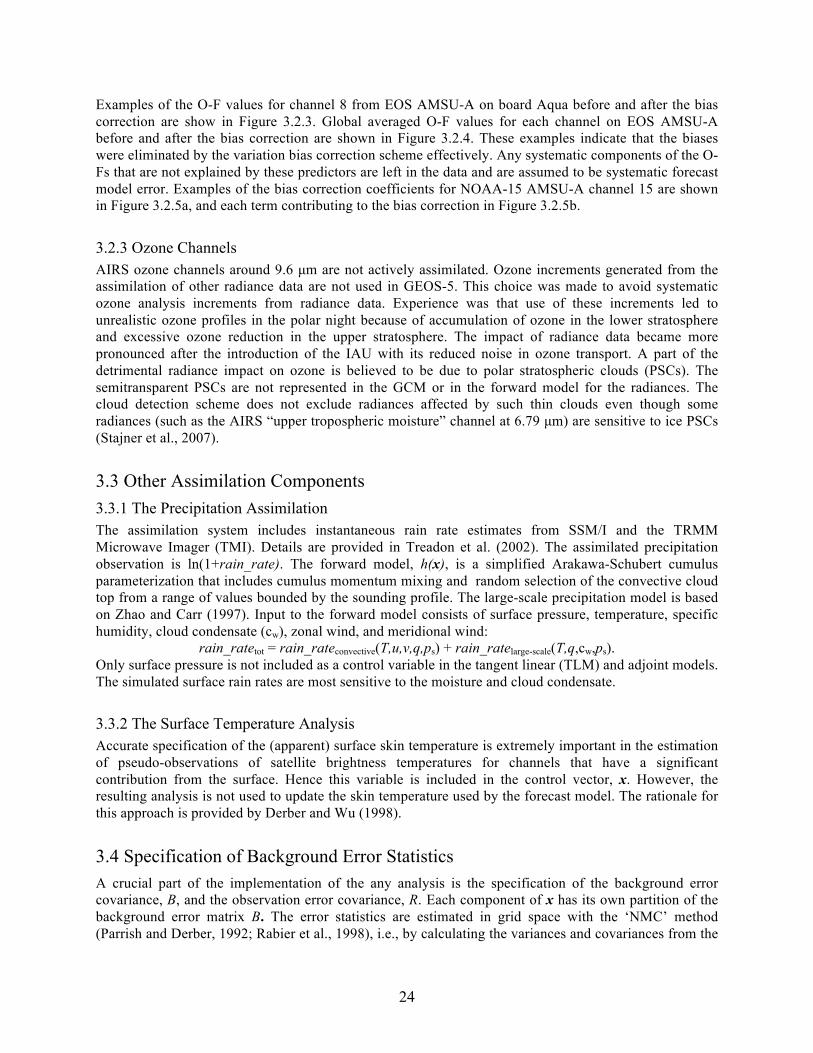
24

Examples of the O-F values for channel 8 from EOS AMSU-A on board Aqua before and after the bias correction are show in Figure 3.2.3. Global averaged O-F values for each channel on EOS AMSU-A before and after the bias correction are shown in Figure 3.2.4. These examples indicate that the biases were eliminated by the variation bias correction scheme effectively. Any systematic components of the O-Fs that are not explained by these predictors are left in the data and are assumed to be systematic forecast model error. Examples of the bias correction coefficients for NOAA-15 AMSU-A channel 15 are shown in Figure 3.2.5a, and each term contributing to the bias correction in Figure 3.2.5b.

3.2.3 Ozone Channels AIRS ozone channels around 9.6 µm are not actively assimilated. Ozone increments generated from the assimilation of other radiance data are not used in GEOS-5. This choice was made to avoid systematic ozone analysis increments from radiance data. Experience was that use of these increments led to unrealistic ozone profiles in the polar night because of accumulation of ozone in the lower stratosphere and excessive ozone reduction in the upper stratosphere. The impact of radiance data became more pronounced after the introduction of the IAU with its reduced noise in ozone transport. A part of the detrimental radiance impact on ozone is believed to be due to polar stratospheric clouds (PSCs). The semitransparent PSCs are not represented in the GCM or in the forward model for the radiances. The cloud detection scheme does not exclude radiances affected by such thin clouds even though some radiances (such as the AIRS “upper tropospheric moisture” channel at 6.79 µm) are sensitive to ice PSCs (Stajner et al., 2007).

3.3 Other Assimilation Components 3.3.1 The Precipitation Assimilation The assimilation system includes instantaneous rain rate estimates from SSM/I and the TRMM Microwave Imager (TMI). Details are provided in Treadon et al. (2002). The assimilated precipitation observation is ln(1+rain_rate). The forward model, h(x), is a simplified Arakawa-Schubert cumulus parameterization that includes cumulus momentum mixing and random selection of the convective cloud top from a range of values bounded by the sounding profile. The large-scale precipitation model is based on Zhao and Carr (1997). Input to the forward model consists of surface pressure, temperature, specific humidity, cloud condensate (cw), zonal wind, and meridional wind:

rain_ratetot = rain_rateconvective(T,u,v,q,ps) + rain_ratelarge-scale(T,q,cw,ps). Only surface pressure is not included as a control variable in the tangent linear (TLM) and adjoint models. The simulated surface rain rates are most sensitive to the moisture and cloud condensate.

3.3.2 The Surface Temperature Analysis Accurate specification of the (apparent) surface skin temperature is extremely important in the estimation of pseudo-observations of satellite brightness temperatures for channels that have a significant contribution from the surface. Hence this variable is included in the control vector, x. However, the resulting analysis is not used to update the skin temperature used by the forecast model. The rationale for this approach is provided by Derber and Wu (1998).

3.4 Specification of Background Error Statistics A crucial part of the implementation of the any analysis is the specification of the background error covariance, B, and the observation error covariance, R. Each component of x has its own partition of the background error matrix B. The error statistics are estimated in grid space with the ‘NMC’ method (Parrish and Derber, 1992; Rabier et al., 1998), i.e., by calculating the variances and covariances from the

25

differences between 24-hour and 48-hour forecasts, forecasts initialized 24 hours apart, verifying at the same time.

3.4.1 State Variables 3.4.1.1 Stream function, u, v, humidity The variance statistics of ψ are shown in Figure 3.4.1 as a function of latitude and sigma level. The error variance (m4 s-2) is larger in mid-latitudes than in the tropics and larger in the southern hemisphere than in the northern. The horizontal scales are larger in the tropics, and increase with height. The vertical scale factors are larger in the mid-latitude, and decrease with height. The vertical scale factors depicted in the figures below represent inputs to the recursive filters used to create the covariance functions. They are such that the vertical correlation generated from the recursive filter fits the scales estimated from the training data sets. The resulting vertical scale of the covariance function varies with height, becoming broader toward the top of the model. For example, see Figure 3.4.2 which shows the vertical correlation for pseudo-relative humidity at different levels, given a constant vertical scale factor of 1.0. The error variances and vertical scales for humidity are shown in Figure 3.4.3.

Figure 3.4.1: Example of estimated background error statistics for ψ. Top: error standard deviation as a function of latitude and sigma level (in m2s-1); middle: horizontal scales of covariance (in km); bottom: vertical scale factor of covariance. Left hand panels are the statistics used for GEOS-5.0.1; right-hand panels for GEOS-5.1.0.

26

Figure 3.4.2: Example of the vertical correlation at different levels, given a constant vertical scale factor of 1.0. This structure is generated by the recursive filter to model the vertical correlation for all variables.

Figure 3.4.3: Example of estimated background error statistics for pseudo-relative humidity. Top: error standard deviation as a function of latitude and sigma level; middle: horizontal scales of covariance (in km); bottom: vertical scale factors for covariance.

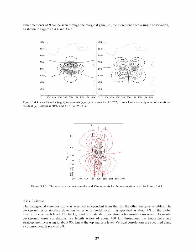
27

Other elements of B can be seen through the marginal gain, i.e., the increment from a single observation, as shown in Figures 3.4.4 and 3.4.5.

Figure 3.4.4: u (left) and v (right) increments (xa–xb), at sigma level 0.267, from a 1 m/s westerly wind observational residual (yo – h(xb)) at 50°N and 330°E at 250 hPa.

Figure 3.4.5: The vertical cross-section of u and T increments for the observation used for Figure 3.4.4. 3.4.1.2 Ozone The background error for ozone is assumed independent from that for the other analysis variables. The background error standard deviation varies with model level: it is specified as about 4% of the global mean ozone on each level. The background error standard deviation is horizontally invariant. Horizontal background error correlations use length scales of about 400 km throughout the troposphere and stratosphere, increasing to about 800 km at the top analysis level. Vertical correlations are specified using a common length scale of 0.8.

28

3.4.1.3 Satellite Bias Correction Coefficients Since the satellite bias correction coefficients are analysis variables, it is necessary to specify the background error variances. These background error variances have been specified in a simple manner by scaling the predictors so that the variances of the various predictors are approximately equal (except the constant predictor) and then applying a constant diagonal matrix for the background errors. The constant used in the background errors gives fairly large weight to the values from the previous analysis.

3.4.2 The Mass-Wind Balance Constraint The specification of the background error covariance matrix is extremely important in any data assimilation system since it is primarily the background error covariance matrix that determines the spreading of information from observations. Despite its importance, the way in which the background error covariance matrix is modeled in any practical assimilation system is dominated by the compromises that must be made in order to produce a viable computational algorithm. Despite the advantages of the GSI in terms of the flexibility in representing the covariance structures, the modeling of the linear mass-wind balance through a linear balance constraint is not straightforward. In the GSI, to avoid the heavy computational burden of solving a Poisson equation at each assimilating level and at each iteration step, balance projections are introduced to link the balanced part of temperature and surface pressure directly with the stream function. The corresponding balance coefficients are estimated together with other background error statistics using the NMC method. This approach is indeed computationally-efficient, however, to ensure good wind-mass coupling, the balance coefficients have to be estimated in such a way to ensure the balanced geopotential height increments, which can be expressed from the balanced temperature and balanced surface pressure, are in good linear balance with the rotational wind increments from the GSI analysis. Otherwise, the balance projections will lead to inappropriate wind-mass coupling in which the information about the mass field will be extracted incorrectly from the wind observations, and vice versa. Since the linear balance equation was not used in the tuning process for the original approach of estimating the balance coefficients, it was found that the resultant balance projections did not adequately model the linear wind-mass balance constraint. A new approach was developed that employs the linear balance equation and hydrostatic relationship to connect the balanced part of the temperature with the stream function, so that the covariance between the stream function and balanced temperature can be derived from the stream function related covariances. The balance coefficients estimated with this new approach ensure the wind-mass balance projections are equivalent to directly applying a linear balance constraint inside the GSI. 3.4.2.1 Linear Mass-Wind Balance Projections in the GSI 3.4.2.1.1 Wind-Mass Balance Projection Coefficients The control variables of the GSI are stream function increments (δψ), unbalanced velocity potential increments (δχunbal), unbalanced virtual temperature increments (δTunbal), unbalanced surface pressure increments (δPunbal) and pseudo-relative humidity increments (δq). Typically the background error statistics for these control variables are estimated from a set of 24/48-hour forecast differences by the NMC method, and in the original implementation of the GSI the balance projection coefficients were estimated from the same set of forecast differences. The linear balance constraint to be satisfied so that the balanced geopotential heights are in good linear balance with the rotational winds is:

€

∇2δΦ=∇ ⋅ f∇δψ( ), where

€

f is the Coriolis parameter and

€

δΦ is the geopotential height that can be expressed as

29

€

δΦ= RδTd lnσ +RTsps

σ1∫ δP (3.4.1)

from the integration over the hydrostatic equation in σ coordinates. In (3.4.1),

€

R is the gas constant,

€

ps and

€

Ts are standard surface pressure and surface temperature, respectively. The balance projections are introduced in the GSI to avoid the time-consuming process of solving the linear balance equation directly. The projections define the balanced part of temperature (δTbal) and surface pressure (δPbal) directly from δψ by assuming

€

δTbalk = νklδψll=1

N∑ ,

δPbal = µll=1

N∑ δψl ,

where νkl are the balance coefficients for δTbal and µl the balance coefficients for δPbal, and N is the number of assimilating levels. The vertical cross-covariance between the stream function at level m and temperature at level k can be constructed as

€

δψm , δTk = δψm , δTbalk +δTunbalk . (3.4.2)

If we assume that there are no correlations between δψ and the unbalanced part of temperature,

€

δTunbalk , then equation (3.4.2) becomes

€

δψm ,δTk = νkll=1

N∑ δψm ,δψl for m =1,...,N and k =1,...,N .

Thus, we have the following linear system of equations for balanced temperature coefficients

€

νk ≡ νk1,νk2,,νkN( )T :

€

Cψνk =ηk , (3.4.3) where

€

Cψ ≡ (<δψm ,δψl >), l =1,…,N ,m =1,…,N is the vertical covariance matrix of δψ, and

€

ηk ≡ (<δψ1,δTk >,<δψ2,δTk >,,<δψN ,δTk >)T the vertical cross-covariance vector between δψ and δT. The matrix (

€

νk , k=1,…,N) forms an N × N coefficient matrix which is latitude dependent. Derived in

the same way, the balance coefficients for surface pressure,

€

µ ≡ µ1,µ2,,µN( )T , can be estimated from the following linear system of equations:

€

Cψµ = ρ, (3.4.4)

where

€

ρ ≡ (<δψ1,δP >,<δψ2,δP >,,<δψN ,δP >)T . The covariance matrix

€

Cψand vectors

€

ηk and

€

ρ are functions of latitude and are usually estimated by the NMC method. Practically,

€

Cψ is a singular matrix or a matrix very close to singular. Instead of solving equation (3.4.3) or (3.4.4) directly,

€

νk and

€

µ

are estimated by finding the pseudo-inverse matrix

€

Cψ+of

€

Cψ . 3.4.2.1.2 Off-line Background Error Covariance Modeling The relation between the mass and the wind through the wind-mass balance projections, are examined through

€

LΦ and

€

Rψ , the left-hand and right-hand sides of the linear balance equation, respectively:

30

€

LΦ =∇2δΦ,Rψ =∇ ⋅ f∇δψ( ).

Using the discrete form of (3.4.1), the covariance between δψ and

€

LΦ can be related to the balanced temperature and balanced surface pressure by

€

δψm ,LΦk = − bnn δψm ,∇2δTbaln + bnn+1 δψm ,∇

2δTbaln+1

n=1

k−1∑ +

RTsps

δψm ,∇2δPbal , (3.4.5)

where

€

bnn ≡ cp( ˜ σ n+1 − ˜ σ n ) /2 ˜ σ n ,

€

bnn+1 ≡ cp( ˜ σ n+1 − ˜ σ n ) /2 ˜ σ n+1,

€

˜ σ ≡σnR /c p ,

€

σn is the

€

σ at the nth interface of the

€

σ layers (

€

σ1 =1), cp is the specific heat at constant pressure. All the analysis variables are defined at the mid-point of each layer. If we substitute the projections for

€

δTbaln and

€

δPbal into (3.4.5), then we can see that the GSI

representation of

€

<δψm ,LΦ > depends on the mass-wind balance coefficients and the representation of

€

<δψ,∇2δψ > . Both

€

<δψ,∇2δψ > and

€

<δψm ,Rψ > are the stream function related covariances that are modeled in the GSI by the recursive filters from the background error statistics for δψ. If δTbal and δPbal satisfy the linear balance equation with δψ, then we have

€

δψm ,LΦk = δψm , Rψk , (3.4.6) and the balance projection scheme introduced in the GSI is equivalent to using the linear balance equation inside the analysis. The balance coefficients should be estimated in such a way as to ensure (3.4.6) is satisfied in the analysis. Otherwise, the balance projections will provide an incorrect wind-mass coupling with information about the mass field extracted incorrectly from wind observations, and vice versa. The linear mass-wind balance is a good first-order approximation in the wind-mass balance modeling, which can be examined by diagnosing

€

<δψm , Rψ > and

€

<δψm ,LΦ > directly from the same set of forecast differences (not shown). 3.4.2.1.3 The Performance of the Original GSI Implementation The wind-mass balance coefficients estimated with the current approach from equations (3.4.3) and (3.4.4) cannot ensure

€

<δψm ,LΦ > and

€

<δψm , Rψ > be close enough to have the correct wind-mass coupling in the analysis. Figure 3.4.6 shows the profiles of

€

<δψm , Rψ > (solid curves) and

€

<δψm ,LΦ > (dashed curves) using equation (3.4.5) from the stream function's background error statistics and the balance coefficients estimated with the original approach with m=23 (σ = 0.5) and at the selected latitudes. We can see that

€

<δψm ,LΦ > and

€

<δψm , Rψ > are quite different, especially in the tropics. In the mid- and high-latitudes and at the certain levels (for example, σ = 0.2), the difference is relatively small (not shown). However, typically there are relatively large differences from 30°S to 30°N no matter which levels are selected. These differences will surely cause incorrect wind-mass coupling in the GSI analysis. This was confirmed by looking at the analysis increments generated exclusively from the wind-mass balance projections. Plots of

€

Rψ and

€

LΦ and their ratio (not shown) indicated that the balance coefficients tuned with the original GSI implementation do not satisfy the linear balance constraint except in parts of the mid-latitude troposphere. The differences between

€

Rψ and

€

LΦ are relatively large in the region from 40°S to about 40°N and from 200 hPa to levels in the stratosphere.

31

Figure 3.4.6: The profiles of

€

< δψ,∇2δΦ > (dashed line) and

€

< δψ,∇ ⋅ ( f ∇δψ) > (solid line) at eight selected latitudes with δψ being at σ = 0.5. These profiles are calculated from the balance projection coefficients estimated according to the original GSI implementation, and values have been multiplied by 103. 3.4.2.2 A new approach for estimating the Linear Mass-Wind Balance Projections A new estimation approach was developed which makes use of the linear balance constraint and the stream function related covariances to ensure that the wind-mass balance projections in the GSI satisfy the linear balance equation. 3.4.2.2.1 Formulation From equation (3.4.5), we have

€

δψm ,LΦk − LΦk+1 = bkk δψm ,∇2δTbalk + bkk+1 δψm ,∇

2δTbalk+1, (3.4.7)

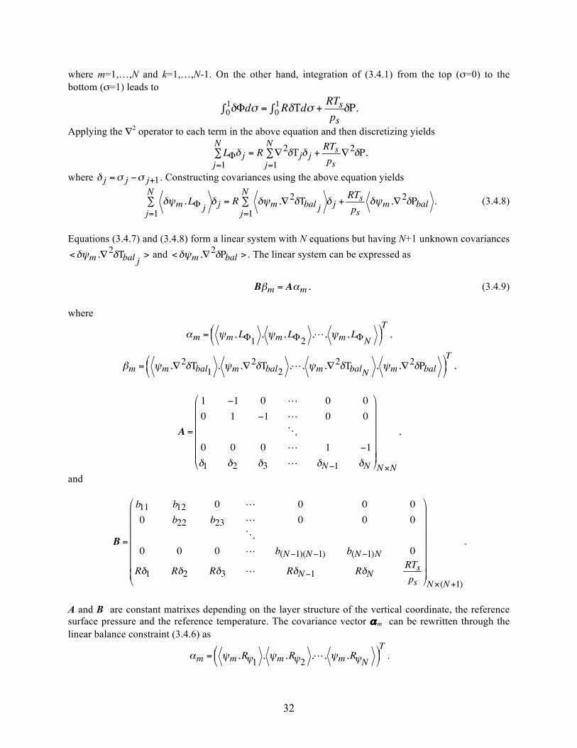
32

where m=1,…,N and k=1,…,N-1. On the other hand, integration of (3.4.1) from the top (σ=0) to the bottom (σ=1) leads to

€

δΦdσ = RδTdσ +RTsps

01∫0

1∫ δP.

Applying the ∇2 operator to each term in the above equation and then discretizing yields

€

LΦj=1

N∑ δ j = R ∇2

j=1

N∑ δTjδ j +

RTsps

∇2δP,

where

€

δ j =σ j −σ j+1 . Constructing covariances using the above equation yields

€

δψm ,LΦ jj=1

N∑ δ j = R δψm ,∇

2δTbal jj=1

N∑ δ j +

RTsps

δψm ,∇2δPbal . (3.4.8)

Equations (3.4.7) and (3.4.8) form a linear system with N equations but having N+1 unknown covariances

€

<δψm ,∇2δTbal j > and

€

<δψm ,∇2δPbal > . The linear system can be expressed as

€

Bβm = Aαm , (3.4.9)

where

€

αm = ψm ,LΦ1 , ψm ,LΦ2 ,, ψm ,LΦN

T,

βm = ψm ,∇2δTbal1 , ψm ,∇

2δTbal2 ,, ψm ,∇2δTbalN , ψm ,∇

2δPbal

T,

€

A =

1 −1 0 0 00 1 −1 0 0

0 0 0 1 −1δ1 δ2 δ3 δN−1 δN

N×N

,

and

€

B =

b11 b12 0 0 0 00 b22 b23 0 0 0

0 0 0 b(N−1)(N−1) b(N−1)N 0

Rδ1 Rδ2 Rδ3 RδN−1 RδNRTsps

N×(N+1)

.

A and B are constant matrixes depending on the layer structure of the vertical coordinate, the reference surface pressure and the reference temperature. The covariance vector αm can be rewritten through the linear balance constraint (3.4.6) as

€

αm = ψm ,Rψ1 , ψm ,Rψ2 ,, ψm ,RψN

T,

33

which are stream function related covariances that can be estimated from the training data sets or replaced by their representation in the GSI through the recursive filters from the stream function's background error statistics. From A, B and αm, the unknown vector βm, which represents the covariance structures between the stream function and balanced part of temperature and surface pressure, can be estimated by

€

βm = B+Aαm , (3.4.10)

where B+ represents the pseudo-inverse matrix of B. One of differences between the new approach and the approach described in the section 3.4.2.1 is that η k in (3.4.3) needs to be estimated independently from the training data sets, while in the new approach, βm is derived from the stream function related covariances. Once we have the covariances

€

<δψm ,∇2δTbalk > and

€

<δψm ,∇2δPbal > for all m and k, the balanced

temperature coefficients vector ν k and surface pressure coefficients µ can be estimated from the following linear equations:

€

ˆ C ψνk = ˆ η k ,ˆ C ψµ = ˆ ρ ,

(3.4.11)

which can be derived in the same way as the equations (3.4.3) and (3.4.4).

€

ˆ C ψ is the N × N covariance

matrix defined as

€

<δψm ,∇2δψl > . It is another stream function related covariance matrix that needs to

be estimated from the training data sets or approximated by the appropriate GSI representation. The vectors in the right sides of equations (3.4.11) are formed from the components of βm in (3.4.10), that is,

€

ˆ η k ≡ δψ1,∇2δTbalk , δψ2,∇2δTbalk ,, δψN ,∇2δTbalk

T

and

€

ˆ ρ ≡ δψ1,∇2δPbal , δψ2,∇2δPbal ,, δψN ,∇2δPbal

T

.

3.4.2.2.2 Estimation of αm and

€

ˆ C ψ From the above formulations, it is clear that the wind-mass balance coefficients from the new estimation approach are dependent on two vertical covariance matrixes, i.e., (α1, α2, …, αN) and

€

ˆ C ψ . These two matrixes can be estimated either directly from the training data sets or indirectly from the stream function background error statistics through the GSI background error covariance modeling. The GSI representations of αm and

€

ˆ C ψ are different from their direct diagnostics from the training data sets. The representation of vertical correlation for the stream function is a near-Gaussian function generated by two self-adjoint recursive filters, and the horizontal correlation is approximated by the superposition of three near-Gaussian kernels with different length scales. Compared with the corresponding direct diagnostics, the GSI representations are smooth and have no remote correlations. To ensure the balance projection scheme is equivalent to using the linear balance constraint inside the GSI, αm and

€

ˆ C ψshould be estimated from the stream function background error statistics. If αm and

€

ˆ C ψ are estimated from the training data sets, then the estimated coefficients with the new approach will make the balanced geopotential height satisfy the linear balance equation with the diagnostic stream function error rather than the corresponding GSI representation since these two are quite different. So the estimation of these new balance coefficients involves the following steps: firstly, tuning the stream function background error statistics from the training data sets, then using an off-line code to calculate αm

34

and

€

ˆ C ψ from those modeled stream function error statistics, and, finally, estimating the βm, ν k and µ from (3.4.10) and (3.4.11). 3.4.2.3 Evaluations of the New Wind-Mass Balance Projections The wind-mass balance coefficients estimated with the new approach are different from those from the original approach described above. Since these coefficients have no clear physical meaning, we will instead compare the resultant balanced temperature and surface pressure. The vertical covariances for the balanced temperature and the surface temperature can be written as

€

δTbalk ,δTball =νkTCψν l ,

δPbal ,δPbal = µTCψµ.

The vertical cross-covariance between these two balanced fields can be expressed as

€

δPbal ,δTbalk = µTCψν l . Since

€

Cψ is an independent matrix, the differences in these covariances only reflect the differences in the balance coefficients. If we replace

€

Cψ with its corresponding GSI modeling, then we have the GSI representation of these covariances. Figure 3.4.7 shows the profiles of the standard deviation of the background balanced temperature error at selected latitudes used in GEOS-5.0.1 and 5.1.0. The resultant balanced temperature error in the upper levels is much smoother in either of the new balance projections (green curves) than in the original projections (red curves). In the tropics, the more balanced temperature can be explained from the stream function in the new projections. While in the original projection, the balanced temperature error at the high latitudes near σ = 0.001 is much larger in the southern hemisphere than in the northern hemisphere. The GSI representation of vertical correlations from the original and the new balance projections are also quite different. Figure 3.4.8 shows the profiles of balanced temperature correlation at σ = 0.5 and at the same latitudes as Figure 3.4.7. With the new balance projections (green curves), the GSI representation of the correlation is much smoother and sharper especially at the low-latitudes, and has no remote correlation. The correlations resulting from the new balance projections have the typical two-sided negative lobes, which is different from those (red curves) from the original projections. The upper negative lobe in the extratropics is stronger than the lower negative lobe, except if σ is at 0.2, when the lower negative lobe is stronger than upper negative lobe (Figure 3.4.9). All of these are typical correlation features found in the temperature field. Figure 3.4.10 shows the profiles of the cross-correlations between the balanced temperature and balanced surface pressure. Again, the new cross-correlation curves (green and yellow curves) are much smoother and retain the major features shown in the red curves. The new wind-mass balance projections are equivalent to using the linear balance constraint inside the GSI. As a parallel to Figure 3.4.6, Figure 3.4.11 shows the profiles of covariances

€

<δψm ,LΦ > (dashed curves) and

€

<δψm , Rψ > (solid curves) with m = 21 (σ = 0.5) based on the new balanced coefficients. In Figure 3.4.11, the differences between

€

<δψm ,LΦ > and

€

<δψm , Rψ > are reduced significantly compared to Figure 3.4.6. The slight differences, especially at the tropical latitudes, are due to poor conditioning of the matrix

€

ˆ C ψ in which some of small singular values have to be removed before the estimation procedure. Figure 3.4.12 shows the zonal averages of absolute value of

€

LΦ (top panel) and

€

Rψ (middle panel) in the northern hemisphere, computed from the related analysis increments with the new wind-mass balance projections. The bottom panel shows that the balance constraint is satisfied over most of the globe. Although the ratio near the equator is slightly larger than 1, it is much reduced from the

35

original implementation; and since the dominant error near the equator is unbalanced, the balance modeling near the equator is not a critical issue. The wind-mass balance from the new projections can also be seen in Figure 3.4.13 which shows the distribution of geopotential height and rotational wind increments. The rotational wind vectors follow the geopotential height lines, and the center of the mass matches the center of the wind very well.

36

Figure 3.4.7: The standard deviation profiles of balanced temperature as a function of sigma at eight selected latitudes. The red curves are the estimates from the original GSI implementation, while the other curves are from the new approach. The green (yellow) curve shows the statistics used in GEOS-5.0.1 (GEOS-5.1.0).

37

Figure 3.4.8: As in Figure 3.4.7, but for the correlation profiles at σ = 0.5.

38

Figure 3.4.9: As in Figure 3.4.7, but for the correlation profiles at σ = 0.2.

39

Figure 3.4.10: As in Figure 3.4.9, but for the cross-correlation profiles between the balanced temperature and balanced surface pressure.

40

Figure 3.4.11a: As in Figure 3.4.6, but from the balanced projections estimated with the new approach used for GEOS.5.0.1.

Figure 3.4.11b: As in Figure 3.4.11a, but for statistics used for GEOS.5.1.0 and only for 10ºS and 10ºN, there being little change at higher latitudes.

41

Figure 3.4.12: Zonal averages of

€

| LΦ |≡ | ∇2δΦ | (top),

€

| Rψ |≡ | ∇ ⋅ ( f ∇δψ) | (middle). LΦ and Rψ are calculated based on the analysis increments which only includes the wind-mass balance projections with the new approach. All the values in the top and middle have been multiplied by 1010. The bottom panel displays the ratio of top field to the middle, the contours of 0.5, 0.75, 0.9, 1.0, 1.1, 1.25, 1.5, 2.0, 4.0, 6.0 are plotted. Left-hand panels are for GEOS-5.0.1; right-hand panels are for GEOS-5.1.0.

42

Figure 3.4.13: The distributions of geopotential height increments and vectors of the rotational wind from the wind-mass balanced projections estimated with the new approach with σ=0.5 (top) and σ=0.1 (bottom). The left-hand panels are for GEOS-5.0.1; right-hand panels for GEOS-5.1.0.

43

3.5 The Observing System and the Observation Error Statistics The data streams currently assimilated by the GEOS-5 DAS are shown in Table 3.5.1. The observation error covariances are all univariate and the auto-covariance terms are delta-functions so that the corresponding entries in the matrix R are diagonal. Global constants (usually varying by level) for the observation error standard deviations used in GEOS-5 are given below in the discussion of each observation.

Table 3.5.1: Input observation data sources and parameters.

Conventional Data Radiosondes u, v, T, q, Ps PIBAL winds u, v Wind profiles u, v Conventional, ASDAR, and MDCRS aircraft reports u, v, T NEXRAD radar winds u, v Dropsondes u, v, T, Ps PAOB Ps

GMS, Meteosat, cloud drift IR and visible winds u, v MODIS clear sky and water vapor winds u, v GOES cloud drift IR winds u, v GOES water vapor cloud top winds u, v Surface land observations Ps Surface ship and buoy observations u, v, T, q, Ps

SSM/I Rain rate, wind speed TMI Rain rate QuikSCAT u, v Satellite Data TOVS 1b Radiances AMSU-A: N15, N16, N18

AMSU-B: N15, N16, N17 MHS: N18 HIRS2: TIROS-N, N6, N7, N8, N9, N10, N11, N12, N14 HIRS3: N16, N17 HIRS4: N18 MSU: TIROS-N, N6, N7, N8, N9, N10, N11, N12, N14 SSU: TIROS-N, N6, N7, N8, N9, N10, N11, N14

EOS/Aqua Level 1b Radiances AIRS (150 channels), AMSU-A SSM/I radiances DMSP-8, DMSP-10, DMSP-11,

DMSP-13, DMSP-14, DMSP-15 (7 channels)

GOES sounder TB GOES-08, GOES-10, GOES-12 Channels 1-18

SBUV2 ozone (Version 8 retrievals) Nimbus 7, NOAA 9, 11, 14, 16, 17

44

3.5.1 Conventional In-situ Upper-Air Data 3.5.1.1 Radiosondes, Dropsondes and Pibals Radiosondes are the predominant source of conventional upper-air data in GEOS-5. They provide temperature, wind and moisture information at mandatory and “significant” levels. The temperature information is assimilated as virtual temperature by the GSI. While radiosonde data are quite valuable, providing profiles of mass and wind information, they are inhomogeneously distributed, favoring land over ocean and the Northern Hemisphere over the Southern Hemisphere. There are also temporal variations in radiosonde soundings, with the majority of observations at 00 and 12 UTC; and only a few locations launching soundings at the other synoptic times. The GEOS-5 analysis uses data from both mandatory and “significant” levels; the observation error is increased for profile observations closely spaced in the vertical. The radiosonde network is augmented to a limited degree by dropsondes (from aircraft) and pilot balloons (which provide low-level wind profiles of lesser accuracy). Dropsondes are instrument packages similar to radiosondes that are dropped from aircraft. The dropsonde transmits information about temperature and humidity to the aircraft, and wind observations can be inferred from the horizontal motion of the dropsonde during its descent. For pilot balloon (PIBAL) observations, a balloon is tracked with an optical theodolite and the elevation and azimuth observations are used with a predetermined ascent rate to calculate winds aloft. The NCEP processing also assigns the PIBAL report type to radiosonde wind reports that are not accompanied by a mass (height/temperature) report. 3.5.1.2 Aircraft Observations Aircraft are another significant source of conventional upper-air temperature and wind observations. These data are also highly inhomogeneous. Although in the vicinity of airports ascent and descent profiles are available, the data are primarily single level observations. Humidity data are collected on a few flights but are not yet used in the assimilation system. Aircraft observations are obtained from manual (AIREP and PIREP) and automated (MDCRS and ASDAR) reports. The automated reports are more accurate and thus are assigned a smaller observation error. 3.5.1.3 Wind Profilers Wind profilers are vertically pointing clear-air Doppler radars that produce wind profiles in the vertical from measurements of energy backscattered by refractive index fluctuations (Hogg et al., 1983). The GSI currently assimilates wind profiler measurements from the NOAA Profiler Network (NPN) in the central U.S. and from a few other profiler sites (primarily in the tropical Pacific) that transmit PIBAL format wind reports over the GTS. Pacific stations have been reporting since about 1990, NPN since May 1992. 3.5.1.4 NEXRAD VAD Winds Doppler radars measure mean radial velocity versus azimuth angle in 360 degree scans around the radar. Wind velocity at various heights are derived from a best-fit sine wave to the radial wind components at given distances from the radar (Klazura and Imy, 1993). Hence, the observation represents the mean wind in a volume about the radar site. These observations are primarily low and mid-level winds and are generated at U.S. NEXRAD (WSR-88D) radar locations.

45

3.5.1.6 Synthetic (BOGUS) Tropical Cyclone winds In the NCEP GDAS processing, if the tropical cyclone vortex relocation program encounters “weak” vortices which could not be used to update the global sigma first guess, the locations of these storms are passed to a subsequent program which then generates synthetic (bogus) wind mandatory level profile reports (throughout the depth of the storm) in the vicinity of the storm(s) to better define tropical systems for the analysis. The GEOS-5 system does not run the program that generates these synthetic wind profiles, but the synthetic observations will be assimilated if they are present in the operational PREPBUFR data received from NCEP.

Table 3.5.2: Observation errors for Radiosonde/Dropsonde ‘mass’ reports.

Temperature (K) Specific Humidity (g/kg) Pressure (hPa) Radiosonde Dropsonde Radiosonde Dropsonde

> 1000 1.30 1.50 0.90 1.10 1000 1.10 1.30 0.80 1.00 950 0.90 1.10 0.80 1.00 900 0.70 0.90 0.80 1.00 850 0.60 0.80 1.00 1.20 800 0.60 0.80 1.10 1.30 750 0.60 0.80 1.30 1.40 700 0.60 0.80 1.30 1.50 650 0.55 0.75 1.30 1.50 600 0.50 0.70 1.30 1.50 550 0.50 0.70 1.30 1.50 500 0.50 0.70 1.30 1.50 450 0.50 0.70 1.30 1.50 400 0.50 0.70 1.30 1.50 350 0.55 0.75 1.30 1.50 300 0.65 0.85 1.30 1.50 250 1.10 1.30 – – 200 1.20 1.50 – – 150 1.20 1.50 – – 100 1.20 1.50 – – 75 1.20 1.50 – – 50 1.20 1.50 – – 40 1.40 – – – 30 1.60 – – – 20 1.85 – – – 10 2.00 – – – 5 2.00 – – – 4 2.00 – – – 3 2.00 – – – 2 2.00 – – – 1 2.00 – – –

< 1 2.50 – – –

46

Table 3.5.3: Observation errors for radiosonde, profiler and VAD wind (m/s).

Pressure (hPa) Radiosonde PIBAL Dropsonde

Profiler from PIBAL rpt NPN Profiler VAD wind

> 1000 1.5 1.5 1.5 1.4 2.0 2.0 1000 1.5 1.5 1.5 1.4 2.0 2.0 950 1.5 1.5 1.5 1.5 2.0 2.0 900 1.5 1.5 1.5 1.5 2.0 2.0 850 1.5 1.5 1.5 1.5 2.0 2.0 800 1.5 1.5 1.5 1.6 2.0 2.0 750 1.6 1.6 1.6 1.6 2.0 2.0 700 1.7 1.7 1.7 1.6 2.0 2.0 650 1.8 1.8 1.8 1.8 2.0 2.0 600 1.9 1.9 1.9 1.9 2.0 2.0 550 2.0 2.0 2.0 2.0 2.0 2.0 500 2.1 2.1 2.1 2.1 2.1 2.1 450 2.2 2.2 2.2 2.3 2.3 2.3 400 2.2 2.2 2.2 2.6 2.6 2.6 350 2.3 2.3 2.3 2.8 2.8 2.8 300 2.3 2.3 2.3 3.0 3.0 3.0 250 2.4 2.4 2.4 3.2 3.2 3.2 200 2.4 2.4 2.4 2.7 2.7 2.7 150 2.4 2.4 2.4 2.4 2.4 2.4 100 2.4 2.4 2.4 2.4 2.1 2.1 75 2.4 2.4 2.4 2.4 2.1 2.1 50 2.4 2.4 2.4 2.4 2.1 2.1 40 2.4 2.4 2.4 2.4 2.1 2.1 30 2.5 2.5 2.5 2.4 2.1 2.1 20 2.7 2.7 2.7 2.4 2.1 2.1 10 2.9 2.9 2.9 2.4 2.1 2.1 5 3.1 3.1 3.1 2.5 2.1 2.1 4 3.3 3.3 3.3 2.6 2.1 2.1 3 3.5 3.5 3.5 2.7 2.1 2.1 2 3.7 3.7 3.7 2.8 2.1 2.1 1 3.9 3.9 3.9 2.9 2.1 2.1

< 1 4.1 4.1 4.1 3.0 2.1 2.1

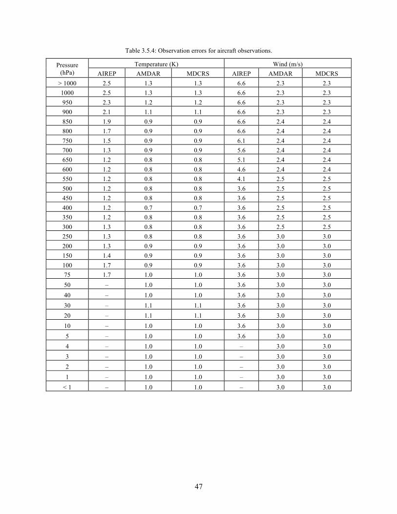
47

Table 3.5.4: Observation errors for aircraft observations.

Temperature (K) Wind (m/s) Pressure (hPa) AIREP AMDAR MDCRS AIREP AMDAR MDCRS

> 1000 2.5 1.3 1.3 6.6 2.3 2.3 1000 2.5 1.3 1.3 6.6 2.3 2.3 950 2.3 1.2 1.2 6.6 2.3 2.3 900 2.1 1.1 1.1 6.6 2.3 2.3 850 1.9 0.9 0.9 6.6 2.4 2.4 800 1.7 0.9 0.9 6.6 2.4 2.4 750 1.5 0.9 0.9 6.1 2.4 2.4 700 1.3 0.9 0.9 5.6 2.4 2.4 650 1.2 0.8 0.8 5.1 2.4 2.4 600 1.2 0.8 0.8 4.6 2.4 2.4 550 1.2 0.8 0.8 4.1 2.5 2.5 500 1.2 0.8 0.8 3.6 2.5 2.5 450 1.2 0.8 0.8 3.6 2.5 2.5 400 1.2 0.7 0.7 3.6 2.5 2.5 350 1.2 0.8 0.8 3.6 2.5 2.5 300 1.3 0.8 0.8 3.6 2.5 2.5 250 1.3 0.8 0.8 3.6 3.0 3.0 200 1.3 0.9 0.9 3.6 3.0 3.0 150 1.4 0.9 0.9 3.6 3.0 3.0 100 1.7 0.9 0.9 3.6 3.0 3.0 75 1.7 1.0 1.0 3.6 3.0 3.0 50 – 1.0 1.0 3.6 3.0 3.0 40 – 1.0 1.0 3.6 3.0 3.0 30 – 1.1 1.1 3.6 3.0 3.0 20 – 1.1 1.1 3.6 3.0 3.0 10 – 1.0 1.0 3.6 3.0 3.0 5 – 1.0 1.0 3.6 3.0 3.0 4 – 1.0 1.0 – 3.0 3.0 3 – 1.0 1.0 – 3.0 3.0 2 – 1.0 1.0 – 3.0 3.0 1 – 1.0 1.0 – 3.0 3.0

< 1 – 1.0 1.0 – 3.0 3.0

48

3.5.2 Satellite Radiance Data Remotely sensed information from satellites typically offers much greater and more isotropic coverage than that from conventional in situ sources. In contrast to GEOS-4, GEOS-5 primarily assimilates satellite level-1b (raw) radiances rather than retrievals. However, single level cloud motion vector winds obtained from geostationary satellite images, precipitation and surface wind speed estimates from microwave sensors, surface wind estimates from scatterometer radar, and column ozone obtained from the SBUV and SBUV/2 instruments are assimilated as retrievals. For level-1b radiance data, the observation-minus-forecast departure statistics (both mean and standard deviation) provide an upper bound of the observation errors as they represent the summed contribution of errors in radiative transfer model, cloud detection, and errors in the background estimate of the atmospheric state. The fit of the GEOS-5 background profiles to the observed radiance for some instrument channels were found smaller than the current assigned values in GSI suggests that the weight currently give to these level-1b radiance data in GSI could be slightly increased. However, it is safer to be conservative and leave the observation error unchanged from the current assigned values. The assigned observation error variances in GSI for each instrument types are listed Appendix A. 3.5.2.1 TOVS/ATOVS The TIROS Operational Vertical Sounder (TOVS) consists of three separate sounding instruments: the High-resolution Infrared Radiation Sounder 2 (HIRS2), later HIRS3 and HIRS4 for advanced TOVS (ATOVS); the Microwave Sounding Unit (MSU), later the Advanced Microwave Sounding Unit (AMSU), and the Microwave Humidity Sounder (MHS); the Stratospheric Sounding Unit (SSU), also replaced by AMSU. The TOVS instruments measure the radiance from Earth passively in different spectral regions specific to each type of remote sensing:

• in CO2 or O2 absorption zones to retrieve the vertical temperature profile, • in water vapor or ozone absorption zones to determine the profiles and total concentrations of water

or ozone, • in zones of low absorption to determine surface parameters.

The measured radiance includes thermal emission in the microwave and infrared channels and reflected solar radiation in the visible and shorter-wavelength infrared channels. Radiance is commonly expressed in terms of equivalent blackbody temperature (brightness temperature), as brightness temperature behaves more linearly with atmospheric temperature and other parameters than does the radiance. TOVS has flown on the TIROS-N satellite and on NOAA operational polar-orbiting environmental satellites (POES) 6-12 and 14. NOAA 10 and 12 did not have an SSU instrument. The Advanced TOVS instrument (ATOVS), consisting of HIRS3 and AMSU, has been launched on the recent series of NOAA satellites; NOAA-15, 16 and 17, and HIRS4, AMSU-A and MHS on the latest, NOAA-18. HIRS2 has one visible channel (0.69 µm), seven shortwave IR channels (3.7 to 4.6 µm), and 12 longwave IR channels (6.5 to 15 µm). The nominal spatial resolution at nadir is 17.4 km. Details of the instrument and data can be found at http://www2.ncdc.noaa.gov/docs/podug/html/c4/sec4-1.htm. The HIRS/3 instrument has one visible channel (0.69 µm), seven shortwave IR channels (3.7 to 4.6 µm), and 12 longwave IR channels (6.5 to 15 µm). The nominal spatial resolution at nadir is 20.3 km in the visible and shortwave IR and 18.9 km in the longwave IR. The HIRS/3 instrument was flown on NOAA-KLM and instrument details are available at http://goespoes.gsfc.nasa.gov/poes/instruments/hirs3.html. HIRS/4 improves on the resolution of HIRS3, with a nominal spatial resolution of 10 km at nadir. Details of the instrument are available at http://goespoes.gsfc.nasa.gov/poes/instruments/hirs4.html. MSU has 4 channels centered near the 57 GHz oxygen cluster. The nominal resolution is 110 km at nadir. For details of the instrument and data go to http://www2.ncdc.noaa.gov/docs/podug/html/c4/sec4-3.htm.

49

The AMSU-A is divided into two physically separate modules: Module A-1 contains 13 channels and Module A-2 contains two channels. AMSU-A1 consists of 12 V-band channels (3 through 14) and one W-band channel (15). AMSU-A2 contains the two lower frequencies (K-band channel 1 and Ka-band channel 2). The nominal resolution is 48 km at nadir. The AMSU-B provides information on water vapor profiles from the Earth’s surface to an altitude of about 200-mb. The highest channels, 18, 19 and 20, span the strongly opaque water vapor absorption line at 183 GHz and provide atmospheric humidity data. Channels 16 and 17, at 89 GHz and 150 GHz, respectively, enable deeper penetration through the atmosphere to the Earth's surface. The spatial resolution at nadir is nominally 16 km. Further details can be found at http://www2.ncdc.noaa.gov/docs/klm/index.htm. The MHS is a five-channel microwave instrument intended primarily to measure profiles of atmospheric humidity. It is also sensitive to liquid water in clouds and measures cloud liquid water content. Because of the high variability of atmospheric water, the MHS has a higher resolution than the AMSU-A, with a nominal resolution of 16 km at nadir. MHS has four humidity channels in the 157 GHz to 190 GHz range. As with AMSU-A, it has a surface-viewing window channel at 89 GHz, partly to ensure cross-registration of the two sounding instruments. See http://goespoes.gsfc.nasa.gov/poes/instruments/mhs.html for further details. The stratospheric sounding unit (SSU) provided by the U.K. Meteorological Office was flown on several NOAA operational meteorological satellites. SSU employs the pressure modulation technique to measure stratospheric emission in 3 channels of the 15 µm CO2 band. The nominal resolution is 147 km at nadir. It is designed to retrieve temperatures in the stratosphere. The SSU has three channels with weighting functions that have peak response at pressure levels of 15, 6, and 2 mb respectively. Details of the instrument and data can be found at http://www2.ncdc.noaa.gov/docs/podug/html/c4/sec4-2.htm. The TOVS/ATOVS observing system is summarized in Table 3.5.5.

Table 3.5.5: Summary of TOVS/ATOVS observing system.

Satellite Pre-launch ID Instruments Orbit Operational Data Coverage

TIROS-N TN HIRS/2, MSU, SSU PM 1978/10/30 --- 1980/06/01

NOAA-06 NA HIRS/2, MSU, SSU AM 1979/07/02 --- 1980/04/17 1985/04/08 --- 1986/11/17

NOAA-07 NC HIRS/2, MSU, SSU PM 1981/07/11 --- 1985/02/19

NOAA-08 NE HIRS/2, MSU, SSU AM 1983/04/26 --- 1984/06/20 1985/07/02 --- 1985/10/14

NOAA-09 NF HIRS/2, MSU, SSU PM 1985/01/02 --- 1988/11/01 NOAA-10 NG HIRS/2, MSU AM 1986/11/25 --- 1991/09/01

NOAA-11 NH HIRS/2, MSU, SSU PM 1988/10/12 --- 1994/12/31 1997/07/15 --- 1999/02/25

NOAA-12 ND HIRS/2, MSU AM 1991/08/18 --- 1997/07/14 NOAA-14 NJ HIRS/2, MSU, SSU AM 1995/01/19 --- 2007/05/22 NOAA-15 NK HIRS/3, AMSU-A, AMSU-B AM 1998/07/02 --- current date NOAA-16 NL HIRS/3, AMSU-A, AMSU-B PM 2001/01/01 --- current date NOAA-17 NM HIRS/3, AMSU-A, AMSU-B AM 2002/07/15 --- current date NOAA-18 NN HIRS/4, AMSU-A, HMS PM 2005/10/01 --- current date

50

3.5.2.2 EOS/Aqua The NASA EOS Aqua spacecraft, launched in May 2002, carries a sounding suite consists of three instruments: the Atmospheric Infrared Sounder (AIRS), the Advanced Microwave Sounding Unit (AMSU) and the Humidity Sounder for Brazil (HSB). All three instruments are cross-track scanners. AIRS is a 2382-channel high-spectral-resolution grating spectrometer, with 2378 channels measuring infrared radiation from 3.7-15.4 µm and four visible channels and near-infrared radiation measuring from 0.4-0.94 µm. AIRS obtains atmospheric temperature and humidity profiles from the surface to an altitude of 40 km. Its infrared measurements have a horizontal spatial resolution of 13.5km at nadir, and its visible and near-infrared measurements have a horizontal spatial resolution of 2.3km at nadir. AIRS is capable of providing high-resolution measurements in the vertical: 1-km layers in the troposphere and 3-5-km layers in the stratosphere. Details of AIRS can be found at http://aqua.nasa.gov/about/instrument_airs.php. AMSU-A on board Aqua is a 15-channel sounder consisting of two physically separate units AMSU-A1 and AMSU-A2. The A1 module contains 13 channels, and the A2 module has 3 channels. Twelve of AMSU-A’s channels, with frequencies between 50 and 60 GHz, are used predominantly for temperature sounding, whereas the other three channels, at frequencies of 23.8, 31.4, and 89 GHz, are used predominantly for water vapor and precipitation measurements. The horizontal resolution of the AMSU-A data at nadir is 40.5 km, three times as coarse as the AIRS data. The AMSU instrument is particularly valuable for providing sounding information below clouds, except for regions with heavy precipitation and optically thick clouds. Details can be found at http://aqua.nasa.gov/about/instrument_amsu.php.

Figure 3.5.1: AIRS observed brightness temperatures for all 2378 channels are shown in light blue. The spectral location (blue diamond), instrument noise (red cross), and the assigned observation errors (green asterisk) in GSI for the 281-channel subset are also shown.

51

HSB is a microwave humidity sounder. It has four channels, one at 150 GHz and the other three measuring at spectral bands centered on a strong water vapor absorption line at 183.31 GHz. HSB is particularly important for accurate humidity profiles under overcast conditions. The horizontal resolution of HSB at nadir is 13.5km. See http://aqua.nasa.gov/about/instrument_hsb.php for more details. Level-1b radiances from AIRS and AMSU-A are used in GEOS-5. The full spectral resolution (2378 channels) AIRS data is too large for the global data assimilation model to digest the information. Therefore, a subset containing 281 channels from the original full spectral resolution set was selected for the NWP centers. This channel selection is listed in Appendix A. The observation errors assigned in the GSI for AIRS along with the instrument noise from the instrument team and their spectral locations are shown in Figure 3.5.1. 3.5.2.3 GOES Sounder Data GOES satellites are in a geosynchronous orbit. Normally, there are two GEOS satellites in operation: GOES-East stationed at 75°W, and GOES-West at 135°W, providing coverage of most of the Western Hemisphere. GOES satellites carry both sounder and imager. Currently, only GOES sounder data are used in GEOS-5 (Table 3.5.6). The GOES sounder instrument has 18 thermal infrared bands plus a low-resolution visible band. The field of view is 8 km and is sampled every 10 km. The GOES sounder spectral selection is very similar to the HIRS instruments carried on the NOAA polar-orbiting satellites. It has six bands in the 15 micron band, two window channels, three mid-tropospheric water vapor bands, one ozone band, and five 4 near infrared band, and a visible band. Details of the instrument can be found at http://goespoes.gsfc.nasa.gov/goes/instruments/i_m_sounder.html.

Table 3.5.6: Summary of GOES satellite operation.

Satellite Launch Date Current Status

GOES-08 (I) 1994/04/13 Stand-by mode GOES-10 (K) 1997/04/25 Operational GOES-West at 135°W GOES-12 (M) 2001/06/23 Operational GOES-East at 75°W

3.5.2.4 SSM/I Radiances The Special Sensor Microwave/Imager (SSM/I) is a passive microwave sensor on the Defense Meteorological Satellite Program (DMSP) satellite series. It has 7 microwave channels at 4 frequencies (19.35 GHz, 22.235 GHz, 37 GHz, and 85.5 GHz), each with dual (vertical and horizontal) polarization (except for the 22 GHz channel). This dual polarization allows the detection of surface properties. The SSM/I has a swath width of about 1400 km with a footprint resolution of 40 km at a spacing of 25 km. The SSM/I radiance data used in GEOS-5 is summarized in Table 3.5.7. Additional information for the instrument is available at http://www.class.noaa.gov/release/data_available/dmsp/index.htm.

Table 3.5.7: Summary of DMSP satellite availability.

Satellite Operational Data Coverage

DMSP-08 (F08) July 1987 --- December 1991 DMSP-10 (F10) December 1990 --- November 1997 DMSP-11 (F11) December 1991 --- May 2000 DMSP-13 (F13) May 1995 --- Current DMSP-14 (F14) May 1997 --- Current DMSP-15 (F15) December 1999 --- August 2006

52

3.5.3 Satellite Retrievals 3.5.3.1 SBUV and SBUV/2 The Solar Backscatter Ultraviolet Instrument (SBUV) on Nimbus-7 and updated SBUV/2 instruments on NOAA POES series of satellites measure Solar irradiance and Earth radiance (from backscattered solar radiation) in the near ultraviolet spectrum. The measurements are taken from sun-synchronous orbits at nadir using 160 km wide field of view over the sunlit part of the Earth. Using ratios of backscattered radiances and solar irradiances at 12 wavelengths total ozone columns and ozone profiles are retrieved. Version 6 retrievals (Bhartia et al., 1996) were used in GEOS-5.0.1. Version 8 retrievals are used in GEOS-5.1.0 and GEOS-5.2.0. Version 8 retrievals (Bhartia et al., 2004) use a priori profiles from the ozone climatology of McPeters et al. (2007) to remove any artificial trends arising from the a priori guess. The vertical resolution of Version 8 retrievals is 6-8 km in the upper stratosphere. Comparison of SBUV/2 Version 8 data with the Stratospheric Aerosol and Gas Experiment II (SAGE II) data shows that most biases are within ±10%, except for larger negative biases near 50 hPa in the Tropics (Terao and Logan, 2007).

Table 3.5.8: SBUV Observation errors.

Level Layer bounds

(hPa) Obs error (Du) 1 0.00-0.24 1.000 2 0.24-0.50 1.000 3 0.50-0.99 1.000 4 0.99-1.98 1.000 5 1.98-3.95 1.000 6 3.95-7.90 1.414 7 7.90-15.81 1.225 8 15.81-31.41 1.225 9 31.41-62.82 1.871

10 62.82-126.66 1.871 11 126.66-253.31 1.732 12 253.31-1013.24 1.414

Total ozone 2.236

3.5.3.2 Cloud-track Winds Cloud-track winds (CTW, also known as cloud-drift winds or atmospheric motion vectors, AMV) are observations derived from sequences of images observed by satellites. The winds are calculated by an objective procedure that selects targets, assigns pressure altitude, and calculates atmospheric motion from the motion of the selected targets in successive images. The GEOS-5 DAS uses cloud-track winds from geostationary satellites produced by NESDIS, JMA, and EUMETSAT; data from these sources provides near global coverage of CTWs equatorward of 60 degrees. CTW from MODIS on the EOS/Terra and Aqua platforms, also produced by NESDIS, provides data primarily in the polar regions.

53

Although the cloud track wind data are not thinned, the ‘prepdata’ processing at NCEP applies data selection based on the value of the quality index assigned to the wind by the data producer. For NESDIS GOES hi-density winds, the quality marker (QM) is based on a recursive filter flag (RFF) value: RFF ≤ 49 QM = 13 (exclude) 49 < RFF ≤ 55 QM = 3 (suspect - GSI inflates the observation error by a factor of 1.2) 55 < RFF ≤ 84 QM = 2 (normal) RFF > 84 QM = 1 (‘keep’ flag, treat as normal). For EUMETSAT BUFR winds, the QM is based on the quality indicator (QI) value, with the QI calculated using forecast background: QI ≤ 0.8 QM = 13 (exclude) QI > 0.8 QM = 2 (normal). The EUMETSAT BUFR winds are produced every 90 minutes. The NCEP processing applies a time window so that only the set of winds produced closest to the synoptic time is retained for use by the assimilation. The EUMETSAT ELW BUFR winds have been included in NCEP operational system since 24 April, 2001. Prior to that NCEP, processed 'SATOB' winds from the GTS and applied similar restrictions with respect to the quality indicator and time window. The observation errors used in the GSI for cloud-tracked winds are provided in Table 3.5.9.

Table 3.5.9: Observation errors for cloud-tracked winds (m s-1).

Pressure (hPa)

NESDIS picture triplet

NESDIS IR

NESDIS WV cloud top

JMA IR/VIS

EUMETSAT IR/VIS MODIS IR MODIS WV

1000 1.8 3.4 6.0 1.8 1.8 3.8 – 950 1.8 3.0 6.0 1.8 1.8 3.8 – 900 1.8 2.7 6.0 1.8 1.8 3.8 – 850 1.8 2.5 6.0 1.8 1.8 3.8 – 800 1.8 2.7 6.0 2.4 1.8 3.8 – 750 1.8 2.8 6.0 2.4 1.8 3.8 – 700 1.9 3.1 6.0 2.4 2.1 3.9 – 650 1.9 3.3 5.5 2.5 2.1 3.9 – 600 2.0 3.4 5.5 3.0 2.1 4.0 – 550 2.0 3.6 5.0 3.5 2.3 4.0 4.0 500 2.1 3.8 5.0 4.0 2.5 4.1 4.1 450 3.0 4.0 5.0 4.5 3.0 5.0 5.0 400 4.0 4.2 5.0 5.0 4.2 6.0 6.0 350 4.3 4.4 5.0 5.0 4.5 6.3 6.3 300 4.6 4.6 5.0 5.0 4.7 6.6 6.6 250 5.0 4.8 5.0 5.0 5.0 7.0 7.0 200 5.0 5.0 5.0 5.0 5.0 7.0 7.0 150 5.0 5.5 5.0 5.0 5.0 7.0 7.0 100 5.0 6.0 5.0 5.0 5.0 7.0 7.0 75 5.0 6.5 6.0 5.0 5.0 7.0 7.0 50 5.0 7.0 7.0 5.0 5.0 7.0 7.0

54

3.5.3.3 Precipitation Estimates SSM/I and TMI yield precipitation estimates over the oceans. These data are subsetted by generating a 1° grid of super-observations. The observational error variance is defined as 1.0 + 0.25× rain_rate. 3.5.3.4 Surface Wind Estimates The GEOS-5 near-real-time product uses the NCEP GDAS data stream. The NCEP GDAS operational processing takes SSM/I wind speed generated by the Neural Net 3 algorithm and superobs them onto a 1° latitude/longitude grid. The QuikSCAT scatterometer data are quality-controlled and then superobed onto a 0.5° grid. For the MERRA system, SSM/I wind speed retrievals are obtained from Remote Sensing Systems (RSS, http://www.ssmi.com/). RSS SSM/I wind speed retrievals are superobed to a 0.5° latitude/longitude grid. The QuikSCAT scatterometer data for the MERRA system are processed as in the GEOS-4 system, selecting data only from the ‘sweet spot’ on each side of the swath and thinning by selecting winds from every other scan position. The observation errors specified for surface winds varies according to the source: SSM/I wind speed 2.0 m/s QuikSCAT winds 2.5 m/s ERS1/2 winds 2.5 m/s Atlas buoy winds 2.2 m/s Surface marine winds 2.5 m/s. Surface marine observations are provided by ships and moored buoys.

3.5.4 Land Surface Observations The GEOS-5 GSI assimilates surface pressure observations from land surface stations. For METAR observations without a surface pressure report, the altimeter setting is used to obtain a surface pressure value. Other land surface observations (temperature, moisture, wind) are kept as passive.

Table 3.5.10: Observation errors for surface pressure (hPa).

Pressure (hPa) Surface marine Surface land Dropsonde METAR

> 1000 1.0 1.0 1.0 1.0 1000 1.0 1.0 1.0 1.0 950 1.0 1.0 1.0 1.0 900 1.0 1.0 1.0 1.0 850 1.0 1.0 1.0 1.0 800 1.0 1.0 1.0 1.0 750 1.0 1.0 1.3 1.3 700 1.1 1.0 1.6 1.6 650 1.2 1.2 – – 600 1.2 1.2 – –

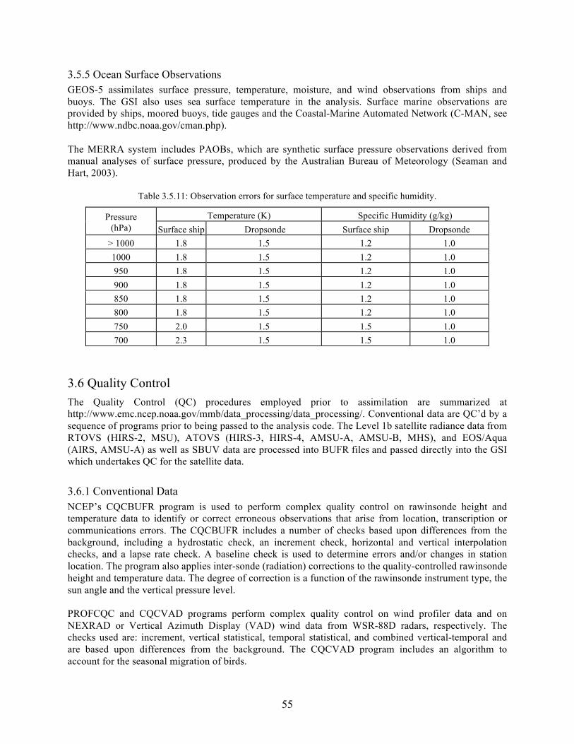
55

3.5.5 Ocean Surface Observations GEOS-5 assimilates surface pressure, temperature, moisture, and wind observations from ships and buoys. The GSI also uses sea surface temperature in the analysis. Surface marine observations are provided by ships, moored buoys, tide gauges and the Coastal-Marine Automated Network (C-MAN, see http://www.ndbc.noaa.gov/cman.php). The MERRA system includes PAOBs, which are synthetic surface pressure observations derived from manual analyses of surface pressure, produced by the Australian Bureau of Meteorology (Seaman and Hart, 2003).

Table 3.5.11: Observation errors for surface temperature and specific humidity.

Temperature (K) Specific Humidity (g/kg) Pressure (hPa) Surface ship Dropsonde Surface ship Dropsonde

> 1000 1.8 1.5 1.2 1.0 1000 1.8 1.5 1.2 1.0 950 1.8 1.5 1.2 1.0 900 1.8 1.5 1.2 1.0 850 1.8 1.5 1.2 1.0 800 1.8 1.5 1.2 1.0 750 2.0 1.5 1.5 1.0 700 2.3 1.5 1.5 1.0

3.6 Quality Control The Quality Control (QC) procedures employed prior to assimilation are summarized at http://www.emc.ncep.noaa.gov/mmb/data_processing/data_processing/. Conventional data are QC’d by a sequence of programs prior to being passed to the analysis code. The Level 1b satellite radiance data from RTOVS (HIRS-2, MSU), ATOVS (HIRS-3, HIRS-4, AMSU-A, AMSU-B, MHS), and EOS/Aqua (AIRS, AMSU-A) as well as SBUV data are processed into BUFR files and passed directly into the GSI which undertakes QC for the satellite data. 3.6.1 Conventional Data NCEP’s CQCBUFR program is used to perform complex quality control on rawinsonde height and temperature data to identify or correct erroneous observations that arise from location, transcription or communications errors. The CQCBUFR includes a number of checks based upon differences from the background, including a hydrostatic check, an increment check, horizontal and vertical interpolation checks, and a lapse rate check. A baseline check is used to determine errors and/or changes in station location. The program also applies inter-sonde (radiation) corrections to the quality-controlled rawinsonde height and temperature data. The degree of correction is a function of the rawinsonde instrument type, the sun angle and the vertical pressure level. PROFCQC and CQCVAD programs perform complex quality control on wind profiler data and on NEXRAD or Vertical Azimuth Display (VAD) wind data from WSR-88D radars, respectively. The checks used are: increment, vertical statistical, temporal statistical, and combined vertical-temporal and are based upon differences from the background. The CQCVAD program includes an algorithm to account for the seasonal migration of birds.

56

The PREPACQC program performs quality control on conventional AIREP, PIREP and AMDAR (Aircraft Report, Pilot Report, Aircraft Meteorological Data Relay) aircraft wind and temperature data. The flight tracks are checked, with bad reports flagged and duplicate reports removed. AIREP and PIREP reports are further quality controlled by comparing isolated reports to the background and flagging outliers flagged and then inter-comparing groups of reports in close geographical proximity using both a vertical wind shear check and a temperature lapse check. The ACARSQC program performs quality control on MDCRS and ACARS aircraft wind and temperature data. Currently only simple data bounds checks are performed. The last program to execute QC before the data are passed to the GSI is OIQCBUFR. It performs an optimum interpolation based quality control on the complete set of observations in the PREPBUFR file. A number of independent checks (horizontal, vertical, geostrophic) are performed using all admitted observations. Each observation is subjected to the optimum interpolation formalism using all observations except itself in each check. A final quality decision (keep, toss, or reduced confidence weight) is made based on the results from all prior platform-specific quality checks and from any manual quality marks attached to the data. For the GEOS-5 real-time forward processing system, the preprocessing QC is performed at NCEP prior to receipt of the data at Goddard. For the MERRA system, the preprocessing QC is conducted at Goddard.

3.6.2 Satellite Radiance Data Quality control procedures depend on the observation type. For the quality control of satellite radiance data, see http://www.emc.ncep.noaa.gov/gmb/treadon/gsi/documents/presentations/1st_gsi_orientation/. HIRS, GOES, AIRS: High frequencies are eliminated during the day for reflected solar radiation contamination. Only cloud-free data are used. Screening is also conducted for the surface window to limit the magnitude of the necessary change in surface emissivity. AMSU-A: Data are screened according to cloud liquid water, the scattering index, and according to the magnitude of the necessary change in surface emissivity. AMSU-B: Data are screened according to the ability to simulate quasi-window channels. MSU: Data are screened according to the ability to simulate channel 1 (for channels 1 and 2). GOES imager: Data are screened according to the clear sky fraction and the brightness temperature standard deviation. SSM/I Radiances: Okamoto and Derber (2006) describe the methodology used for assimilation of SSM/I radiances in the GSI. SSM/I radiances are only assimilated over ocean; observations over land or ice are excluded. The QC of the SSM/I 1b radiances is based on the scattering index, si85, the difference between an estimate of the 85V brightness temperature from the other channels with the observed temperature (Ferraro, 1997). Over the ocean, the scattering index is: si85 = [-174.4 + 0.715 Tb19V + 2.439 Tb22V – 0.00504 (Tb22V)2 ] – Tb85V and over the land: si85 = [451.9 - 0.44 Tb19V - 1.775 Tb22V + 0.00574 (Tb22V)2] - Tb85V.

57

Rain is detected if si85 > 10 and this information is used for data thinning and QC. Other checks are based on cloud liquid water (clw), a range check (70 < Tb < 320, for each channel), and a polarization check that (Vpol – Hpol) < -2 for each channel. The clw checks use a clw retrieval (after Weng et al., 1997) from the 85 GHz channels as the first priority, from the 19 GHz channels as the next priority, and then from the 37 GHz channel if the others are not available. For example, clw85 = -0.44 [ log(290.-Tb85H) + 1.11 – 1.26 (log(290. – Tb22V)]. Cloud liquid water estimates are used in data selection/thinning when si85 is not available. The SSM/I radiances are also subject to a gross check on the observation increment, rejecting those with absolute value greater than 3σo, where σo is the specified standard deviation of observation error. Common procedures: The quality control procedure common to all satellite data types is performed by a combination of two tests, a gross check and a check against the predicted values from nearby observations (a buddy check). Gross check: For each observation location, an observation quality parameter is set based on the expected observational error variance for that channel. This quality control parameter is modified by the position across the track of the scan, whether it is over land, sea, snow, sea ice or a transition region, the elevation, the difference between the model and the real orography, and the latitude (the criterion is made tighter in the tropics). For the HIRS channels, the criterion is stricter if the observation is designated partly cloudy by NESDIS, if the differences between selected window channel observations or the simulated window channels are too large, and for the shortwave channels if the solar zenith angle is small. Some of the modifications are designed to eliminate observations that are contaminated, and some to eliminate situations where the simulated observations are deficient. The observation quality parameter is then compared to the difference between the true and simulated observations. The observation is rejected if the difference from the simulated observation is greater than three times the observation quality parameter. The buddy check: At the same time, the observation is compared to a simple interpolation of nearby observational increments to the observation location. The observation is rejected if its difference from the simulated observation and the difference between the interpolated increments and the observation increment are both greater than the observation quality parameter. To minimize the number of observations that are rejected due to errors in nearby observations, the checking is repeated three times with only the observations that have passed the previous time through the quality control check being used for the interpolation of increments. This procedure allows the re-acceptance of some observations that were rejected in the previous passes through the data. The data rejections are performed independently for each channel. Thus, the rejection of one lower tropospheric HIRS channel because of possible cloud contamination does not necessarily result in the rejection of other tropospheric HIRS channels at the same location. This quality control procedure has some known deficiencies and probably rejects some good data in order to ensure the removal of all the bad data.

3.6.3 Precipitation Data The quality control procedures for precipitation observations are outlined in Treadon et al. (2002). Because of the large boundary layer sensitivity of the convective scheme, a smoothness check is added to the data pre-processing. Those observations for which the vertical derivative of the sensitivity profile exceeds a given tolerance are not assimilated. The check flags about 5% of the SSM/I data and 4% of the TMI data. A time screening is also applied to the observations. As the analysis relative time of the observation increases, the quality control error bounds smoothly decrease to zero. The quality control bounds also

58

decrease to zero for observations poleward of 45° latitude. Observations are not used over snow-covered land, ice covered water, and poleward of 60° latitude. These surface type and latitude checks screen out 15.6% of the SSM/I data (0.6% for TMI). Finally, those observations that deviate from the background rain rate by more than three times the estimated observation error are not assimilated.

3.7 The Radiative Transfer Model GEOS-5 versions to GEOS-5.2.0 uses the prototype version of the Community Radiative Transfer Model (pCRTM) for all satellite radiance data except for the historical SSU data stream input for MERRA. The GLATOVS radiative transfer model (Susskind et al., 1983) is used for the SSU. The CRTM, developed under the auspices of the JCSDA, is integrated with the GSI. It is documented at http://www.orbit.nesdis.noaa.gov/smcd/spb/CRTM/ and in Han et al. (2006). The CRTM is comprised of various components involved in simulating satellite radiances. The four main components are: • Atmospheric gaseous absorption • Scattering and absorption by cloud and aerosols • Surface optics – emissivity and reflectivity • The radiative transfer solution.

3.7.1.1 The Gaseous Absorption Model The operational gaseous absorption model used is Compact OPTRAN. The channel or spectral-response function convolved transmittance is modeled as

€

Tch = Tch,wTch,o* Tch,d

*

where

€

Tch,w is the water vapor transmittance, and

€

Tch,o* and

€

Tch,d* are the effective transmittances of

ozone and dry gas (McMillan et al., 1995), respectively. The transmittance component on the right hand side of the above equation is calculated as

€

Tch,g (Ag ) = exp(− kch,g ( ′ A g )0

Ai∫ d ′ A g ) ,

where

€

Ag is the integrated amount of water vapor, ozone, or dry gas, and

€

kch,g is the channel absorption coefficient of water vapor, ozone, or dry gas.

€

kch,g is predicted as

€

ln(kch,g (Ag )) = cg,0(Ag ) + cg, jj=1

6∑ (Ag )xg, j (Ag );

cg, j (Ag ) = ag, j,nn=0

N∑ ln(Ag )

n ,

where the

€

xg, j are predictors such as temperature and pressure and the

€

ag, j,n are constants obtained through regression. Minor gases that are generally well mixed such as CO2, CO, N2O, CH4, CFCs, N2, O2, are not included as state variables but are fixed. Water vapor and ozone are generally not well-mixed and are included as variable gases. 3.7.1.2 The Cloud Absorption and Scattering Model Currently, cloud and precipitation optical parameters are calculated with general Mie theory using a modified gamma distribution function. Several types of hydrometers including cloud ice, cloud liquid

59

water, snow, graupel, hail and rainwater are included. Parameters such as extinction coefficients, single scattering albedo and phase matrix elements are pre-calculated and stored in a lookup table. This table is searched with particle mean size and cloud water content. Absorption and scattering by aerosols are under development. 3.7.1.3 Surface Emissivity and Reflectivity Models The CRTM employs a suite of microwave (MW) and infra-red (IR) surface emissivity and reflectivity models for land, ocean, ice and snow-covered surfaces. Microwave:

• The MW land emissivity model (LandEM) computes land surface emissivity for various surface types, including snow, deserts and vegetation using the two-stream radiative approximation (Weng et al., 2001). The model takes satellite zenith angle, microwave frequency, soil moisture content, vegetation fraction, soil temperature, land surface temperature and snow depth as inputs and computes surface emissivity at vertical (V) and horizontal (H) polarizations.

• The empirical snow and ice emissivity models compute the emissivity via a combination of satellite window channel observations and emissivity databases collected from ground-based MW instruments (Yan et al., 2004). The emissivity databases contain sets of emissivity spectral data measured at a zenith view angle of 50 degrees for various surface types. The window channel observations are used to identify the snow or ice surface type that best describes the surface condition observed. After a spectrum is identified, it is adjusted for the requested zenith angle.

• The MW emissivity over the ocean surface is computed using FASTEM-1 (English and Hewison, 1998). It takes the satellite zenith angle, water temperature, surface wind speed, and frequency as model inputs and computes surface emissivity at V and H polarizations.

Infrared:

• Over the ocean the Infra-Red Sea surface Emissivity (IRSSE) model (van Delst and Wu, 2000) utilizes a lookup table of sea surface emissivities derived from the emissivity model for a wind-roughened sea surface (Wu and Smith, 1997). The lookup table variables are zenith angle (67 entries from nadir to 66.5°), frequency (153 entries from 600 to 3000 cm-1), and wind speed (23 entries from 0 to 15 m/s). Linear interpolation is performed between the lookup table values.

• Over land surfaces, a look-up table is used for the 24 surface types in Table 3.7.1 using the emissivity database of Carter et al. (2002). The database contains surface reflectance measurements as a function of wavelength in both visible and IR spectral regions for these surface types. The emissivity is calculated from the reflectance under the assumption of a Lambertian surface in the IR spectral region.

3.7.1.4 The Radiative Transfer Solver The radiative transfer (RT) solver module solves the RT equation for given atmospheric optical depth profile, surface emissivity and reflectivity, cloud optical parameters and source functions. The clear and cloudy cases are treated with different methods, allowing a simple and efficient solution under the clear-sky condition. For cloudy cases, the radiative transfer is solved with the advanced doubling-adding method (Liu and Weng, 2006), in which fast algorithms are applied to compute layer source function and vertical radiative transfer integration. The CRTM includes the forward and Jacobian models, as well as the Tangent-linear and Adjoint models. The forward model simulates satellite observed radiances. The Jacobian model computes radiance derivatives with respect to the input state variables.

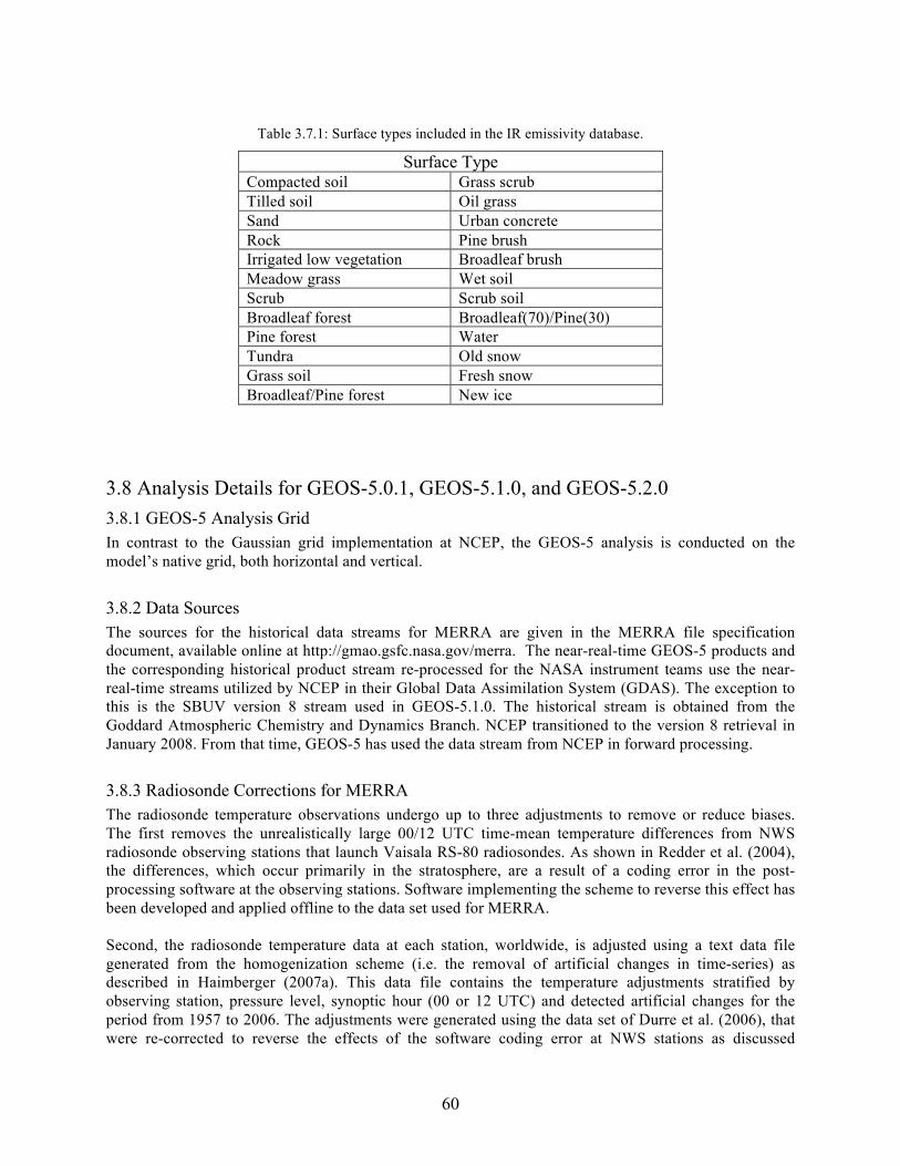
60

Table 3.7.1: Surface types included in the IR emissivity database.

Surface Type Compacted soil Grass scrub Tilled soil Oil grass Sand Urban concrete Rock Pine brush Irrigated low vegetation Broadleaf brush Meadow grass Wet soil Scrub Scrub soil Broadleaf forest Broadleaf(70)/Pine(30) Pine forest Water Tundra Old snow Grass soil Fresh snow Broadleaf/Pine forest New ice

3.8 Analysis Details for GEOS-5.0.1, GEOS-5.1.0, and GEOS-5.2.0 3.8.1 GEOS-5 Analysis Grid In contrast to the Gaussian grid implementation at NCEP, the GEOS-5 analysis is conducted on the model’s native grid, both horizontal and vertical.

3.8.2 Data Sources The sources for the historical data streams for MERRA are given in the MERRA file specification document, available online at http://gmao.gsfc.nasa.gov/merra. The near-real-time GEOS-5 products and the corresponding historical product stream re-processed for the NASA instrument teams use the near-real-time streams utilized by NCEP in their Global Data Assimilation System (GDAS). The exception to this is the SBUV version 8 stream used in GEOS-5.1.0. The historical stream is obtained from the Goddard Atmospheric Chemistry and Dynamics Branch. NCEP transitioned to the version 8 retrieval in January 2008. From that time, GEOS-5 has used the data stream from NCEP in forward processing.

3.8.3 Radiosonde Corrections for MERRA The radiosonde temperature observations undergo up to three adjustments to remove or reduce biases. The first removes the unrealistically large 00/12 UTC time-mean temperature differences from NWS radiosonde observing stations that launch Vaisala RS-80 radiosondes. As shown in Redder et al. (2004), the differences, which occur primarily in the stratosphere, are a result of a coding error in the post-processing software at the observing stations. Software implementing the scheme to reverse this effect has been developed and applied offline to the data set used for MERRA. Second, the radiosonde temperature data at each station, worldwide, is adjusted using a text data file generated from the homogenization scheme (i.e. the removal of artificial changes in time-series) as described in Haimberger (2007a). This data file contains the temperature adjustments stratified by observing station, pressure level, synoptic hour (00 or 12 UTC) and detected artificial changes for the period from 1957 to 2006. The adjustments were generated using the data set of Durre et al. (2006), that were re-corrected to reverse the effects of the software coding error at NWS stations as discussed

61

previously (see Haimberger, 2007b). Finally, the radiosonde temperatures are further adjusted to account for the effects of seasonal changes in the sun's elevation angle and, therefore, radiation bias of the thermistor. The annual average effects of the solar radiation are assumed to be implicitly accounted for in the adjustments generated by the homogenization scheme. The seasonal departures are estimated first by calculating the solar elevation angle at a given station location and observation time on the given date and on the date of the vernal (or autumnal) equinox. The radiation biases are then computed using the most recent version of the table generated at NCEP, and the difference is taken as an estimate of the seasonal departure.

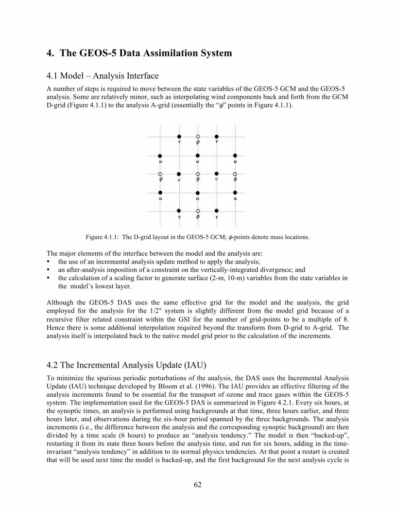
62

4. The GEOS-5 Data Assimilation System

4.1 Model – Analysis Interface A number of steps is required to move between the state variables of the GEOS-5 GCM and the GEOS-5 analysis. Some are relatively minor, such as interpolating wind components back and forth from the GCM D-grid (Figure 4.1.1) to the analysis A-grid (essentially the “φ” points in Figure 4.1.1).

Figure 4.1.1: The D-grid layout in the GEOS-5 GCM; φ-points denote mass locations.

The major elements of the interface between the model and the analysis are: • the use of an incremental analysis update method to apply the analysis; • an after-analysis imposition of a constraint on the vertically-integrated divergence; and • the calculation of a scaling factor to generate surface (2-m, 10-m) variables from the state variables in

the model’s lowest layer. Although the GEOS-5 DAS uses the same effective grid for the model and the analysis, the grid employed for the analysis for the 1/2° system is slightly different from the model grid because of a recursive filter related constraint within the GSI for the number of grid-points to be a multiple of 8. Hence there is some additional interpolation required beyond the transform from D-grid to A-grid. The analysis itself is interpolated back to the native model grid prior to the calculation of the increments.

4.2 The Incremental Analysis Update (IAU) To minimize the spurious periodic perturbations of the analysis, the DAS uses the Incremental Analysis Update (IAU) technique developed by Bloom et al. (1996). The IAU provides an effective filtering of the analysis increments found to be essential for the transport of ozone and trace gases within the GEOS-5 system. The implementation used for the GEOS-5 DAS is summarized in Figure 4.2.1. Every six hours, at the synoptic times, an analysis is performed using backgrounds at that time, three hours earlier, and three hours later, and observations during the six-hour period spanned by the three backgrounds. The analysis increments (i.e., the difference between the analysis and the corresponding synoptic background) are then divided by a time scale (6 hours) to produce an “analysis tendency.” The model is then “backed-up”, restarting it from its state three hours before the analysis time, and run for six hours, adding in the time-invariant “analysis tendency” in addition to its normal physics tendencies. At that point a restart is created that will be used next time the model is backed-up, and the first background for the next analysis cycle is

63

saved. This first 6-hour run is referred to as the “corrector” segment of the IAU. The run is then continued without an analysis tendency for another six hours, saving the other two backgrounds needed by the next analysis – one at the next synoptic time and another at the end of the six hours. This 6-hour run is referred to as the “predictor” segment of the IAU. The entire cycle is then repeated for subsequent synoptic times. Note that during each of the four daily analysis cycles the model is run for 12 hours.

Figure 4.2.1: A schematic of the IAU implementation.

Except for the analyses themselves, all products from GEOS-5 are produced as model histories during the corrector run segment. The sequence of corrector segments (follow the green line in the figure) is a continuous model run, with the extra forcing term from the analysis tendencies. The analysis tendencies do change abruptly every six hours, but state variables are continuous (within the model’s time step) solutions of the equations of motion, albeit with the extra forcing term.

4.3 Balancing Vertically Integrated Mass Divergence from Analysis Increments At each analysis time the DAS produces both a background state and an analysis state of the prognostic wind v and pressure p fields. Defining the mass- or pressure-weighted variables

€

v* = vΔpD =∇ •v *

where Δp is the pressure thickness of the model layer, we can define the analysis increment of mass-divergence as

€

ΔD = DA −DB . Here the subscripts A and B refer to the analysis and background states, respectively. The mass-divergence vertically integrated from the model surface to the model top is equal to the time tendency of the model's surface pressure. While the surface pressure time tendency of the background state is usually small (due to the inherent dynamical balancing properties of the model integration), the implied tendency from the analysis may be significantly large due to errors arising from uncertainties in the observations and error statistics as well as compromises made within the analysis algorithm.

64

Figure 4.3.1: The vertically integrated mass-divergence (in arbitrary units) on 1 August, 2006 for the background (top), the analysis state (middle) and from the difference, or analysis increment (bottom).

65

Figure 4.3.2: Surface pressure for the background and analysis states (upper panels). Also shown are the vertically integrated mass-divergence (arbitrary units) of the background (left-hand lower panel) and the (analysis-background) difference (right-hand lower panel).

Figure 4.3.3: Surface pressure tendency of the background (left-hand upper panel) and analysis states (right-hand upper panel), and the resulting surface pressure after 15 minutes of model integration from the background without analysis (left-hand lower panel) and from the analysis (right-hand lower panel).

66

In the vertically integrated mass-divergence for a typical background state, the largest tendencies occur near high topography, as expected, while the ocean values are quite small (Figure 4.3.1). The vertically integrated mass-divergence from the analysis state exhibits large coherent values covering the entire globe. These imbalances produce surface pressure tendencies on the order of 100 hPa per 6-hours in the first few timesteps, giving rise to large-scale pressure oscillations and wind adjustments. Figure 4.3.2 shows the surface pressure for the background and analysis states, and the corresponding vertically integrated mass divergence for the area near Cuba and the Caribbean Islands on 1 August, 2006. Of particular interest is the low pressure center associated with Tropical Storm Chris. While the analysis was able to enhance and strengthen the initial condition associated with Chris, it left behind a state that contains very strong large-scale imbalances as evidenced by the vertically integrated mass divergence increment. Figure 4.3.3 shows the surface pressure time tendency (calculated from the model's first time-step), in addition to the surface pressure after 15 minutes of model integration. The surface pressure time tendency is consistent with the vertically integrated mass divergence shown previously, and results in the low pressure center completely disappearing after the 15 minutes of integration. Thus, the analysis in this case produced an atmospheric state that was unsustainable by the model dynamics.

4.3.1 The Minimization Algorithm To inhibit this computational adjustment due to the imbalances within the analysis state, we wish to find the smallest change to the analysis increment of mass-divergence (in a least-squares sense) such that the vertically integrated mass-divergence increment vanishes. In doing so, we will only make adjustments to the analysis wind field. Noting that:

€

ΔD − ΔDo = (DA −DB ) − (DAo −DB )

= (DA −DAo ),

where the subscript o refers to the initial guess, we may define the functional F as

€

F = 12l=1

LM∑

DAl −DAolα

2+ λ (DAl

l=1

NM∑ −DBl ).

Here

€

(DAl −DAol ) /α is the penalty function of the analyzed mass-divergence that we want to minimize, λ is a Lagrange multiplier used to enforce the strong constraint of vanishing vertically integrated mass-divergence increment, LM is the total number of model levels, and α is an arbitrary scaling parameter. Taking the first variation of F yields

€

δF = 12l=1

LM∑

DAl −DAolα l

δDAα l

+δλ (DAll=1

NM∑ −DBl ) + λ DAl

l=1

NM∑

or, combining terms,

€

δF = 12l=1

LM∑

DAl −DAolα l2 + λ

δDA +δλ (DAl

l=1

NM∑ −DBl ).

Since δDA and δλ are arbitrary, minimization occurs when their coefficients are equal to zero:

€

DAl −DAolαl2 + λ

= 0,

67

and

€

(DAll=1

NM∑ −DBl ) = 0.

Solving the above equations, we find:

€

DA = DAo − λα2,

λ =DAo − DB∑∑

α 2∑.

4.3.1.1 Case 1: α = 1 With no scaling, the adjustment made is simply a constant applied uniformly in height:

€

DA = DAo − λ ,

λ =DAo − DB∑∑

LM.

However, since adjustments will be made through the winds only, large wind changes are possible near the top of the model where the pressure thickness is very small. 4.3.1.2 Case 1: α = Δp Here we normalize the penalty term by the pressure thickness, yielding:

€

DA = DAo − λ(Δp)2,

λ =DAo − DB∑∑

(Δp)2∑.

We see that the adjustment is applied with a pressure scaling, resulting in small increments near the top of the model. 4.3.1.3 Case 1:

€

α = DAo −DB

Here we normalize the penalty term by the initial mass-divergence increment, yielding:

€

DA = DAo − λ(DAo −DB )2,

λ =DAo − DB∑∑

(DAo −DB )2∑.

Here the magnitude of the adjustment is proportional to the local analysis increment of mass-divergence. Therefore, if the analysis made no local adjustment to the mass-divergence, the updated value will remain unchanged.

4.3.2 Wind Adjustment Algorithm We may write the updated mass-divergence as:

€

DA = DAo +ΔDA , where, as shown above:

68

€

ΔDA = −λα 2. Expressing the adjusted mass-divergence as an adjusted mass-weighted velocity potential:

€

ΔDA =∇2Δχ*, we can then construct the adjusted mass-weighted divergent wind components as:

€

Δuχ* = 1

a cosφ∂∂λ

Δχ*,

Δvχ* = 1a

∂∂φ

Δχ *.

These wind increments are then added to the original mass-weighted analysis winds, and subsequently de-scaled to arrive at the final winds produced by the balancing algorithm:

€

ufinal = (uA* + Δuχ

* ) /ΔpA ,

v final = (vA* + Δvχ

* ) /ΔpA .

4.3.3 Results In all cases the vertically integrated increment of mass divergence is forced to vanish (within truncation). Figure 4.3.4 illustrates this by comparing the zonal mean of the absolute value of the vertically integrated mass divergence increment from the standard analysis with the corresponding analysis after balancing (Case 3). Case 1 and Case 2 show nearly identical results. However, the manner in which the increment of vertically integrated mass divergence is made to vanish is quite different between the various cases. Plots of the zonal mean horizontal wind divergence (Figure 4.3.5) show that in general that the background state and subsequent analyses have significant divergence near the model top, and a secondary maximum near 200 hPa. Case 1, however, shows a pathological divergence field near model top due to the inability of Case 1 to scale its adjustments. Case 2 and Case 3 produce divergence fields quite similar to the standard analysis and background states. Plots of the zonal mean of the analysis increment of divergence (Figure 4.3.6) again highlight the inherent problems associated with Case 1, while Case 2 and Case 3 look quite reasonable. Case 3 shows a substantial impact on the overall divergence pattern around 200 hPa. Figure 4.3.7 shows the zonal mean of the adjustment made to the control analysis of horizontal divergence. Case 1 makes extremely large adjustments in the upper levels of the model which, when mass-weighted, tend to produce the desired vertically integrated result. Cases 2 and 3 tend to produce changes that are more localized in the troposphere. Case 2 applies small mass-weighted changes uniformly in the vertical, while Case 3 applies somewhat larger adjustments in regions associated with large analysis increments. Finally, the forecasts after 15 minutes of integration using the balanced analysis states corresponding to Case 2 and Case 3 are shown in Figure 4.3.8, together with the original forecasts from the background and the control analysis. It should again be noted that the initial condition of the mass field for all the analysis states were identical. Only the divergent components of the winds were modified for the analysis cases 1 and 2. We see that the forecasts initialized from the balanced analysis states were better able to preserve the low pressure associated with Tropical Storm Chris than the original control analysis.

69

Figure 4.3.4: Zonal mean of the absolute value of the vertically integrated mass divergence analysis increment. Figure 4.3.5: The zonal mean horizontal wind divergence (plotted on constant pressure surfaces) of the background state (from the model first guess) and the corresponding results from the analysis states.

Control Analysis Balanced Analysis

70

Figure 4.3.6: The zonal mean of the analysis increment of divergence.

Figure 4.3.7: The zonal mean of the adjustment made to the control analysis of horizontal divergence.

71

Figure 4.3.8: Surface pressure after 15 minutes of model integration, initialized from the background and analysis states (Control, Case 2, and Case 3).

72

5. GEOS-5 Development and Product Version History

5.1 The Versions The versions that have been in production at the time of this document are described below. GEOS-5.0.1: The interim operational version of the GEOS-5 DAS, used to generate early products for the Aura instrument teams. GEOS-5.1.0: Addressed deficiencies noted in GEOS-5.0.1 as well as tuning and development issues for the Modern Era Retrospective-analysis for Research Applications (MERRA, e.g., Bosilovich et al., 2006). This system has undergone a formal validation procedure. The validation results will be documented in a separate technical report. This system was used to support the EOS Aura science team reprocessing effort. The changes from GEOS-5.0.1 are documented below. GEOS-5.2.0: Addressed deficiencies noted in GEOS-5.1.0 in high latitudes. This is the system used for MERRA, to support the ARCTAS field campaign and the CERES science team. The changes from GEOS-5.1.0 are documented below. From 5.0.1 to 5.1.0, substantial changes have been made to both the atmospheric general circulation model (dynamics and physics modules) and analysis system. These modifications operate in concert to impact virtually all output product fields. It is therefore impossible to identify or attempt to quantify one-to-one correspondences between individual system changes and the resulting impacts on the fields. It is clear, however, that the product quality has increased overall, with notable substantial improvements in several key aspects. These include a significantly reduced easterly bias in the upper tropospheric zonal wind along the equator, improved distribution and mean values of precipitation in both the tropics and mid-latitude storm tracks, reduced biases in various land surface quantities, and the elimination of spurious oscillations in both the mid-tropospheric temperature fields at middle to high latitudes and the near-top model level temperature fields near the north pole. The 5.2.0 system addresses a deficiency in the diurnal cycle in the high latitudes.

5.2 The Updates 5.2.1 The Updates in 5.1.0 Updates to the GCM Updates to the Dynamics Module 1) Correction for reproducibility of results in the case of the model being run on different processor

layouts. 2) The Polar Filter has been switched to use an FFT poleward from about 45 degrees (rather than an FFT

near the poles and an algebraic version farther away from poles). The new Polar Filter was implemented to fix a problem encountered if the stratospheric jet crossed the pole during N. Hemisphere Winter.

3) A new computation of U10M and V10M were implemented to represent 10-meter winds better, assuming neutral stability.

4) A new calculation of diagnostic OMEGA was implemented to be more consistent with the calculated rate of change of kinetic and potential energies.

73

Updates to the Physics Modules 1) Corrected ALBEDO boundary conditions, using new albedo data sets. 2) Changed Land-Ice Albedo to 0.75. 3) Reduced re-evaporation over land, so that it is the same as over sea. 4) Placed a lower limit of 0.4 on the Reynolds number 5) Decreased the roughness for heat over bare soil (for values of Leaf Area Index < 0.3) 6) Fixed out-of-bounds array in IR radiation routine. 7) Added protection for LOG(DZ...) in Catchment for thinner levels. 8) Limits on the Reynolds Number over ocean grid points were implemented. The upper limit was

changed from 1000 to 50; the lower limit changed from 0.4 to 0.1. 9) The topography data sets have been modified by multiplicative factors to adjust the global mean value

to 231.5 m (which is the mean of GTOPO30). 10) The MOIST CRF parameter MAX_RI was changed from 110 × 10-6 to 75 × 10-6 to increase the

short/long-wave cloud radiative forcing in the mid-levels in the mid-latitude ice clouds. 11) The RAS relaxation timescale was changed from one time step (20 minutes) to 12 hrs. 12) An upper limit of 2 was imposed on the Richardson Number. 13) Modifications were made to include different heat diffusivities over land and over high topography. 14) The autoconversion rate was increased above 700 hPa. 15) The bounds for the relative humidity ramp for mass flux in RAS were increased from [0.3,0.4] to

[0.6,0.8]. 16) The temperature perturbation in convective boundary layers was capped at 2 K. Updates to the Land Surface Module 1) Updates were implemented to the catchment soil thermal conductivity calculation. 2) The surface layer's heat capacity was reduced outside of tropical forests. 3) A snow energy accounting variable (HSNACC) was added to output diagnostics. HSNACC accounts

for, among other things, the fact that the snowpack (but not the atmosphere) must treat differences in the energy content of snow falling at different temperatures. (HSNACC is an improved version of the older variable HCORR, which had, in the older model only, been added to SHFLUX.)

4) The WCHANGE and ECHANGE variables were added to output diagnostics. These variables are, respectively, the change over the timestep of the total water (in kg/m2s) and total energy (in W/m2) in the land surface element.

5) Minor issues related to energy and water budget accounting were corrected. 6) Minor issues were corrected in the snow code (initialization of snowpack during first snowfall, and

re-layering). 7) The snow thickness over glaciers has been fixed at 4 m. 8) The capacity of canopy interception reservoir was increased by a factor of 5. Updates to the GCM-Analysis Interface 1) Switched from FFT to simple average for D-grid to A-grid transform. 2) Fixed a bug in v-wnd in D-grid to A-grid and A-grid to D-grid transforms. 3) Snow-water-equivalent background file provided for CRTM emissivity calculation in GSI (instead of

snow depth) 4) Changes in the grid point land/water/ice definition needed for the Radiative Transfer Model and for

QC. The grid point is defined as a water grid point if the water fraction of the grid box is > 0.6. The grid point is defined as sea-ice if it is a water grid point and either the ice fraction is > 0.5 or the surface temperature is < -1.7 C.

5) Updated output routines to handle double precision value for longitude.

74

Updates to the Analysis 1) Updated to new background error statistics. These new statistics provide an improved mass-wind

balance in the tropics and reduce the background error variance for balanced temperature at the lowest model levels over the globe.

2) Implemented QC bug fix for MODIS, tightening the tolerance on the gross check quality control to appropriate values.

3) MODIS deep-layer clear-sky winds added to input observation stream (after 2006). 4) The CQCVAD routine was added to provide quality control checks for Doppler VAD winds. 5) Because of background biases, the following microwave channels, which are sensitive to surface

properties, have been excluded over snow, ice and mixed surface types: AMSU-A channels 1-6 and 15; MSU channels 1 and 2; AMSU-B channels 1, 2 and 5.

6) A bug fix was implemented for EOS-AMSU-A emissivity calculation. The EOS AMSU-A bug was a logic error that resulted in EOS AMSU-A using a default emissivity calculation instead of the EOS AMSU-A-specific calculation.

7) The changing temperature lapse rate option is invoked for the satellite bias correction estimation. 8) A vortex re-locator was implemented for tropical cyclones (only). The utility re-positions identified

tropical cyclone vortices in the background (model guess) field, in accordance with their observed locations as determined by the National Hurricane Center. Only the position of the vortex position, and not its intensity, is explicitly altered by this utility. The re-positioning improves the use of appropriate observations in the vicinity of the storm and provides a better initial state for the forecast.

9) The satellite bias angle correction file was updated for data from 2001 forward. 10) The channel selection was updated for AQUA/AIRS and AMSU-B on NOAA-15. 11) The impact of all the radiance data on ozone was excluded. 5.2.1 The Updates in 5.2.0 Updates to the GCM Updates to the Physics Module 1) A bug in cloudnew.F90 related to the use of the wind shear pdf was corrected. 2) Updates were made in cloudnew.F90 to allow a) thicker cold low-level cloud and b) lower limits on

RH in re-evaporation. 3) The upper limits on RADQL and RADQI were lowered to 1 g/kg from 40 g/kg. 4) A bug in MOIST was fixed to pressure weight DTDTFRIC. 5) TROPP_THERMAL, TROPP_EPV, and TROPP_BLENDED options were implemented for

tropopause pressure. 6) Moved updating of FR in GEOS_CatchGridComp.F90 to AFTER DTS and DQS computations. This

provided consistency with the LSM calculations and prevented excessively large DTS and DQS values.

7) Budgets computed in catchment.f90 were fixed. 8) Protections against negative values of Q2M, Q10M, SPHU, OX, EKM and EKH were implemented. 9) The bounds for the relative humidity ramp for mass flux in RAS were changed from [0.6,0.8] to

[0.5,0.65]. 10) The temperature perturbation in convective boundary layers was capped at 2 K over the ocean and 4

K over the land. 11) Corrections were made to ALBEDO and SLRSFC calculations in GEOS_SolarGridComp.F90 and

sorad.F. 12) The historical CO2 record is used.

75

13) A gravity wave drag heating correction based on energy conversion from waves (rather than mean flow) was implemented.

14) A bug was fixed in PCHEM for time-interpolation of climatology aerosols. 15) The θ to T conversion in PHYSICS (from MOIST) is done using a P**KAPPA calculation consistent

with that in MOIST. Updates to the Land Surface Module 1) The LANDICEALBEDO was changed to 0.775 (from 0.8). 2) Modifications were made to thermal capacity of ice to allow a diurnal cycle of surface temperature

over land and sea ice. Updates to the Analysis 1) The satellite bias correction was turned off for AMSU-A channel 14 and SSU channel 3. 2) The IR channels with sensitivity to surface temperature greater than 0.005 are excluded over non-

water surfaces. The channel selection is dynamic, depending on the meteorological background state. The CRTM adjoint is used to estimate the sensitivity.

3) CRTM coefficients for AMSU and MSU, all channels for NOAA-8, and SSU channels for NOAA-11 were updated.

4) A bug was fixed in the quality control of Aqua AMSU-A. 5) The re-calibrated MSU Channel 3 data set from NCEP is used.

76

5.3 The Impacts Some insight into the impacts of the changes are provided below in the average difference fields between selected products.

Figure 5.3.1: Mean sea-level pressure for January 2006. The left-hand figure shows GEOS-5.1.0 (upper panel), 5.0.1 (middle panel) and the difference (5.1.0 minus 5.0.1). The mean difference is 0.05 hPa, the standard deviation of the difference is 0.40 hPa. The right-hand figure shows GEOS-5.2.0 (upper panel), 5.1.0 (middle panel) and the difference (5.2.0 minus 5.1.0). The mean difference is 0.05 hPa, the standard deviation of the difference is 0.35 hPa.

77

Figure 5.3.2: As in Figure 5.3.1, but for 500-hPa height. The mean difference is between 5.1.0 and 5.0.1 is 3.2 hPa, and the standard deviation of the difference is 6.2 hPa. The mean difference is between 5.2.0 and 5.1.0 is 2.9 hPa, and the standard deviation of the difference is 3.3 hPa.

78

Figure 5.3.3: Mean difference in precipitation for January 2006 (upper panels) and July 2004 (lower panels) in mm/day. The left-hand panels show GEOS-5.1.0 minus GEOS-5.0.1. The right-hand panels show GEOS-5.2.0 minus GEOS-5.1.0.

79

Figure 5.3.4: Zonal mean temperature (K) for January 2006. The left-hand figure shows GEOS-5.1.0 (upper panel), 5.0.1 (middle panel) and the difference (5.1.0 minus 5.0.1, lower panel). The right-hand figure shows GEOS-5.2.0 (upper panel), 5.1.0 (middle panel) and the difference (5.2.0 minus 5.1.0, lower panel).

80

Figure 5.3.5: As in Figure 5.3.4, but zonal mean specific humidity (g/kg).

81

Figure 5.3.6: As in Figure 5.3.4, but zonal mean zonal wind (m s-1).

82

6. References Bacmeister, J.T., M.J. Suarez, and F.R. Robertson, 2006: Rain re-evaporation, boundary-layer/convection interactions and Pacific rainfall patterns in an AGCM, J. Atmos. Sci., 8, SRef-ID: 1607-7962/gra/EGU06-A-08925. Bhartia, P.K., R.D. McPeters, C.L. Mateer, L.E. Flynn, and C. Wellemeyer , 1996: Algorithm for the estimation of vertical ozone profiles from the backscattered ultraviolet technique. J. Geophys. Res., 101, 18,793–18,806. Bhartia, P.K., C.G. Wellemeyer, S.L. Taylor, N. Nath, and A. Gopalan, 2004: Solar Backscatter Ultraviolet (SBUV) Version 8 profile algorithm, in Proceedings of the XX Quadrennial Ozone Symposium, edited by C. Zerefos, pp. 295–296, Univ. of Athens, Greece. Bloom, S., L. Takacs, A. DaSilva, and D. Ledvina, 1996: Data assimilation using incremental analysis updates. Mon. Wea. Rev., 124, 1256-1271. Bloom, S., A. da Silva, D. Dee, M. Bosilovich, J.-D. Chern, S. Pawson, S. Schubert, M. Sienkiewicz, I. Stajner, W.-W. Tan, M.-L. Wu, 2005: Documentation and Validation of the Goddard Earth Observing System (GEOS) Data Assimilation System - Version 4. NASA Technical Report Series on Global Modeling and Data Assimilation 104606, v26, 181pp. Boone, A., F. Habets, J. Noilhan, and 20 others, 2004: The Rhone-aggregation land surface scheme intercomparison project: an overview. J. Climate, 17, 187-208. Bosilovich, M. G., S.D. Schubert, M. Rienecker, R. Todling, M. Suarez, J. Bacmeister, R. Gelaro, G.-K. Kim, I. Stajner, and J. Chen, 2006: NASA’s Modern Era Retrospective-analysis for Research and Applications. U.S. CLIVAR Variations, 4 (2), 5-8. Bowling, L.C., D.P. Lettenmaier, B. Nijssen, J. Polcher, R.D. Koster, and D. Lohmann, 2003: Simulation of high latitude hydrological processes in the Torne-Kalix basin, PILPS Phase 2(e), 3, Equivalent model representation and sensitivity experiment, J. Global Planet. Change, 38, 55-71. Carter, C., Q. Liu, W. Yang, D. Hommel, and W. Emery, 2002: Net heat flux, visible/infrared imager/radiometer suite algorithm theoretical basis document. Available at http://npoesslib.ipo.noaa.gov/u_listcategory_v3.php?35. Chin, M., P. Ginoux, S. Kinne, B.N. Holben, B.N. Duncan, R.V. Martin, J.A. Logan, A. Higurashi, and T. Nakajima, 2002: Tropospheric aerosol optical thickness from the GOCART model and comparisons with satellite and sunphotometer measurements, J. Atmos. Sci., 59, 461-483. Chou, M.-D. and M.J. Suarez, 1999: A Solar Radiation Parameterization for Atmospheric Studies. NASA Technical Report Series on Global Modeling and Data Assimilation 104606, v15, 40pp. Chou, M.-D., M.J. Suarez, X.Z. Liang, and M.M.-H. Yan, 2001: A Thermal Infrared Radiation Parameterization for Atmospheric Studies. NASA Technical Report Series on Global Modeling and Data Assimilation 104606, v19, 56pp.

83

Colarco, P.R., A. da Silva, M. Chin, T. Diehl, and R. Govindaraju, 2008: Global Aerosol Distributions from the Online GOCART/GEOS-4 Model and Comparisons to Satellite, Sun Photometer, and In situ Measurements, draft ms for J. Geophys. Res. Collins, N., G. Theurich, C. DeLuca, M. Suarez, A. Trayanov, V. Balaji, P. Li, W. Yang, C. Hill, and A. da Silva, 2005: Design and implementation of components in the Earth System Modeling Framework. Int. J. High Perf. Comput. Appl., 19, 341-350, DOI: 10.1177/1094342005056120. Courtier, P., J.-N. Thépaut, A. Hollingsworth, 1994: A strategy for operational implementation of 4D-Var, using an incremental approach. Quart. J. Roy. Meteorol. Soc., 120, 1367-1388. Dee, D.P., 2004: Variational bias correction of radiance data in the ECMWF system. Proc. ECMWF workshop on assimilation of high spectral resolution sounders in NWP. Reading, UK, 28 June-1 July 2004, 97-112. Dee, D.P., 2005: Bias and data assimilation. Quart. J. Roy. Meteorol. Soc., 131, 3323-3343. Del Genio, A.D., M.S. Yao, W. Kovari, and K.K.W. Lo, 1996: A prognostic cloud water parameterization for global climate models. J. Clim., 9, 270-304. Derber, J. C., R. J. Purser, W.-S. Wu, R. Treadon, M. Pondeca, D. Parrish, and D. Kleist, 2003: Flow-dependent Jb in a global grid-point 3D-Var. Proc. ECMWF annual seminar on recent developments in data assimilation for atmosphere and ocean. Reading, UK, 8-12 Sept. 2003. Derber, J. C., and W.-S. Wu, 1998: The use of TOVS cloud-cleared radiances in the NCEP SSI analysis system. Mon. Wea. Rev., 126, 2287-2299. Dirmeyer, P. A., X. Gao, M. Zhao, Z. Guo, T. Oki, and N. Hanasaki, 2006: GSWP-2, Multimodel analysis and implications for our perception of the land surface. Bull. Am. Met. Soc., 87, 1381-1397. Ducharne, A., R.D. Koster, M.J. Suarez, M. Stieglitz, and P. Kumar, 2000: A catchment-based approach to modeling land surface processes in a GCM, Part 2, Parameter estimation and model demonstration, J. Geophys. Res., 105, 24823-24838. Durre, I., R.S. Vose, and D.B. Wuertz. 2006: Overview of the integrated global radiosonde archive. J. Clim.,19, 53-68. English, S.J. and T.J. Hewison, 1998: A fast generic millimetre wave emissivity model. Microwave Remote Sensing of the Atmosphere and Environment Proc. SPIE, 3503, 22-30. Eyre, J.R., G. Kelly, A.P. McNally, E. Andersson, and A. Persson, 1993: Assimilation of TOVS radiances through one dimensional variational analysis. Quart. J. Roy. Meteorol. Soc., 119, 1427–1463. Ferraro, R.R., 1997: Special Sensor Microwave Imager derived global rainfall estimates for climatological applications. J. Geophys. Res., 102, 16715-16736. Fleming, E.L., C.H. Jackman, D.B. Considine, and R.S. Stolarski, 2001: Sensitivity of tracers and a stratospheric aircraft perturbation to two-dimensional model transport variations. J. Geophys. Res., 106, 14245-14263.

84

Garcia, R.R. and B.A. Boville, 1994: Downward control of the mean meridional circulation and temperature distribution of the polar winter stratosphere, J. Atmos. Sci., 51, 2238–2245. Haimberger, L., 2007a: Homogenization of radiosonde temperature time series using innovation statistics, J. Clim., 20, 1377-1403. Haimberger, L., 2007b: Inclusion of radiation correction developed by NASA for Vaisala RS80 radiosondes operated by US, Report: RSHOM-NOTIZ Nr. 9, 5pp. Han, Y., P. van Delst, Q. Liu, F. Weng, B. Yan, R. Treadon and J. Derber, 2006: JCSDA Community Radiative Transfer Model (CRTM) - Version 1, NOAA Tech Report 122. Hogg, D.C., M.T. Decker, F.O. Guiraud, K.B. Earnshaw, D.A. Merritt, K.P. Moran, W.B. Sweezy, R.G. Strauch, E.R. Westwater, and C.G. Little, 1983: An automatic profiler of the temperature, wind and humidity in the troposphere. J. Climate Appl. Meteor., 22, 807-831. Klazura, G.E., and S.A. Imy, 1993: A description of the initial set of analysis products available from the NEXRAD WSR-88D system. Bull. Amer. Meteor. Soc., 74, 1293-1311. Koster, R. and M. Suarez, 1996: Energy and Water Balance Calculations in the Mosaic LSM, NASA Technical Report Series on Global Modeling and Data Assimilation 104606, Vol. 9. Koster, R.D., M.J. Suárez, A. Ducharne, M. Stieglitz, and P. Kumar, 2000: A catchment-based approach to modeling land surface processes in a GCM, Part 1, Model Structure. J. Geophys. Res., 105, 24809-24822. Langematz, U., 2000: An estimate of the impact of observed ozone losses on stratospheric temperature. Geophys. Res. Lett., 27, 2077-2080. Lawrence, M.G., and P.J. Crutzen. 1998: The impact of cloud particle gravitational settling on soluble trace gas distributions. Tellus Series B, 50, 263-289. Le Treut, H., Z.A. Li, and M. Forichon, 1994: Sensitivity of the LMD general-circulation model to greenhouse forcing associated with 2 different cloud-water parameterizations. J. Clim., 7, 1827-1841. Lin, S.-J., 2004: A vertically Lagrangian finite-volume dynamical core for global models. Mon. Wea. Rev., 132, 2293-2307. Liu, Q, and F. Weng, 2006: Advanced doubling-adding method for radiative transfer in planetary atmospheres. J. Atmos. Sci., 63, 3459- 3465. Lock, A.P., A.R. Brown, M.R. Bush, G.M. Martin, and R.N.B. Smith, 2000: A new boundary layer mixing scheme. Part I: Scheme description and single-column model tests. Mon. Wea. Rev., 138, 3187-3199. Louis, J., M. Tiedtke, and J. Geleyn, 1982: A short history of the PBL parameterization at ECMWF. Proc. ECMWF Workshop on Planetary Boundary Layer Parameterization, Reading, United Kingdom, ECMWF, 59–80. McFarlane, N.A., 1987: The effect of orographically excited gravity wave drag on the general circulation of the lower stratosphere and troposphere. J. Atmos. Sci., 44, 1775-1800.

85

McMillin, L.M., L. J. Crone, M.D. Goldberg, and T.J. Kleespies, 1995: Atmospheric transmittance of an absorbing gas. 4. OPTRAN: a computationally fast and accurate transmittance model for absorbing gases with fixed and variable mixing ratios at variable viewing angles. Appl. Opt. 34, 6269 - 6274. McNally, A.P., J.C. Derber, W.-S. Wu and B.B. Katz, 2000: The use of TOVS level-1B radiances in the NCEP SSI analysis system. Quart. J. Roy. Meteorol. Soc., 126, 689-724. McPeters, R. D., G. J. Labow, and J. A. Logan, 2007: Ozone climatological profiles for satellite retrieval algorithms. J. Geophys. Res., 112, D05308, doi:10.1029/2005JD006823. Moody, E.G., M.D. King, S., Platnick, C.B. Schaaf, and F. Gao, 2005: Spatially complete global spectral surface albedos: Value-added data sets derived from Terra MODIS land products. IEEE Trans. Geosci. Remote Sens., 43, 144–158. Moorthi, S., and M.J. Suarez, 1992: Relaxed Arakawa-Schubert, A Parameterization of Moist Convection for General-Circulation Models. Mon. Wea. Rev. 120, 978-1002. Okamoto, K., and J. Derber, 2006: Assimilation of SSM/I radiances in the NCEP global data assimilation system. Mon. Wea. Rev., 134, 2612-2631. Parrish, D.F., and J.C. Derber, 1992: The National Meteorological Center's Spectral Statistical-interpolation Analysis System. Mon. Wea. Rev., 120, 1747-1763. Pawson, S., I. Stajner, S.R. Kawa, H. Hayashi, W. Tan, J.E. Nielsen, Z. Zhu, L.-P. Chang, N.J. Livesey, 2007: Stratospheric Transport Using Six-Hour Averaged Winds from a Data Assimilation System. J. Geophys. Res., 112, D23103. DOI:10.1029/2006JD007673. Purser, R.J., W.-S. Wu, D.F. Parrish, and N.M. Roberts, 2003a: Numerical aspects of the application of recursive filters to variational statistical analysis. Part I: Spatially homogeneous and isotropic Gaussian covariances. Mon. Wea. Rev., 131, 1524-1535. Purser, R.J., W.-S. Wu, D.F. Parrish, and N.M. Roberts, 2003b: Numerical aspects of the application of recursive filters to variational statistical analysis. Part II: Spatially inhomogeneous and anisotropic general covariances. Mon. Wea. Rev., 131, pp. 1536-1548. Rabier, F., A. McNally, E. Anderson, P. Courtier, P. Unden, J. Eyre, A. Hollingsworth, and F. Bouttier, 1998: The ECMWF implementation of three-dimensional variational assimilation (3D-Var). II: Structure functions. Quart. J. Roy. Meteorol. Soc., 124, 1809-1829. Randel, W.J., F. Wu, J.M. Russell, A. Roche, and J.W. Waters, 1998: Seasonal cycles and QBO variations in stratospheric CH4 and H2O observed in UARS HALOE data. J. Atmos. Sci., 55, 163-185. Redder, C.R., J.K. Luers, and R.E. Eskridge, 2004: Unexplained discontinuity in the U.S. radiosonde temperature data, Part II: Stratosphere. J. Atmos. Ocean. Tech., 21, 1133-1144. Reichle, R., and R.D. Koster, 2005: Global assimilation of satellite surface soil moisture retrievals into the NASA Catchment land surface model. Geophys. Res. Lett., 32, L02404, DOI:10.1029/2004GL021700.

86

Reichle, R.H., R.D. Koster, P. Liu, S.P.P. Mahanama, E.G. Njoku, and M. Owe, 2007: Comparison and assimilation of global soil moisture retrievals from AMSR-E and SMMR. J. Geophys. Res, 112, D09108. DOI: 10.1029/2006JD008033. Reynolds, C.A., T.J. Jackson, and W.J. Rawls, 1999: Estimating available water content by linking the FAO soil map of the world with global soil profile databases and pedo-transfer functions. Proceedings of the AGU 1999 Spring Conference, Boston, MA. May 31-June 4, 1999. Reynolds, R.W., N.A. Rayner, T.M. Smith, D.C. Stokes and W. Wang, 2002: An improved in situ and satellite SST analysis for climate. J. Clim., 15, 1609-1625. Rotstayn, L.D., 1997: A physically based scheme for the treatment of stratiform clouds and precipitation in large-scale models. 1. Description and evaluation of the microphysical processes. Quart. J. Roy. Meteorol. Soc., Part A, 123, 1227-1282. Seaman R., and Hart T., 2003: The history of PAOBs in the Bureau of Meteorology. Aust. Met. Mag., 52, 241-250. Sellers, P.J., Y. Mintz, Y.C. Sud, and A. Dalcher, 1986: A simple biosphere model (SiB) for use within general circulation models. J. Atmos. Sci., 43, 505-531. Simmons, A., 2000: Assimilation of satellite data for Numerical Weather Prediction: basic importance, concepts and methods. Proc. ECMWF seminar on exploitation of the new generation of satellite instruments for numerical weather prediction. Reading, UK, 4-8 September 2000, pp. 21-46. Smith, R.N.B., 1990: A scheme for predicting layer clouds and their water content in a general circulation model. Q. J. Roy. Meteorol. Soc., Part B, 116: 435–460. Stajner, I., C. Benson, H.-C. Liu, S. Pawson, N. Brubaker, L.-P. Chang, L.P. Riishojgaard, and R. Todling, 2007: Ice Polar Stratospheric Clouds Detected from Assimilation of Atmospheric Infrared Sounder Data. Geophys. Res. Lett, 34, L16802, doi:10.1029/2007GL029415. Stajner, I., N. Winslow, R.B. Rood, S. Pawson, 2004: Monitoring of observation errors in the assimilation of satellite ozone data. J. Geophys. Res., 109, No. D6, D06309 doi:10.1029/2003JD004118. Stieglitz, M., A. Ducharne, R.D. Koster, and M.J. Suarez, 2001: The impact of detailed snow physics on the simulation of snow cover and subsurface thermodynamics at continental scales. J. Hydromet., 2, 228-242. Sud, Y., and G.K. Walker, 1999: Microphysics of Clouds with the Relaxed Arakawa Schubert Scheme (McRAS). Part I: Design and Evaluation with GATE Phase III Data. J. Atmos. Sci. 56, 3196-3220. Sundqvist, H., 1978: A parameterization scheme for non-convective condensation including prediction of cloud water content. Quart. J. Roy. Meteor. Soc., 104, 677-690. Susskind, J., J. Rosenfield, and D. Reuter, 1983: An accurate radiative transfer model for use in the direct physical inversion of HIRS and MSU temperature sounding data. J. Geophys. Res., 88, 8550-8568. Tao, W.-K., S. Long, J. Simpson, C.-H. Sui, B. Ferrier, and M.-D. Chou, 1996: Cloud-radiation mechanisms associated with a tropical and a mid-latitude squall line. J. Atmos. Sci., 53, 2624-2651.

87

Terao, Y., and J. A. Logan, 2007: Consistency of time series and trends of stratospheric ozone as seen by ozonesonde, SAGE II, HALOE, and SBUV(/2). J. Geophys. Res., 112, D06310, doi:10.1029/2006JD007667. Treadon, R.E., H.-L. Pan, W.-S. Wu, Y. Lin, W.S. Olson, and R.J. Kuligowski, 2002: Global and Regional Moisture Analyses at NCEP. Proc. ECMWF/GEWEX Workshop on Humidity Analysis, 8-11 July 2002, 33-47. van Delst, P.F.W. and Wu, X., 2000: A high resolution infrared sea surface emissivity database for satellite applications. Technical Proceedings of The Eleventh International ATOVS Study Conference, Budapest, Hungary, 20-26 September 2000, 407-411. Verdin, K.L., and S.K. Jenson, 1996: Development of continental scale DEMs and extraction of hydrographic features, in Proceedings: National Center for Geographic Information and Analysis (NCGIA) International Conference/Workshop on Integrating GIS and Environmental Modeling, Santa Fe, New Mexico, January 21-25, 1996. Verdin, K.L., and J.P. Verdin, 1999: A topological system for delineation and codification of the Earth's river basins, J. Hydrol., 218, 1-12. Weng, F., N. C. Grody, R. R. Ferraro, A. Basist, and D. Forsyth, 1997: Cloud liquid water climatology from the Special Sensor Microwave Imager. J. Clim. 10, 1086-1096. Weng, F., B. Yan, and N. Grody, 2001: A microwave land emissivity model, Geophys. Res., 106, 20,115-20,123. Wilbur, A. C., D. P. Kratz, and S. K. Gupta, 1999: Surface emissivity maps for use in satellite retrievals of longwave radiation. NASA Tech. Memo. TP-1999-209362, 30 pp. Wu, W.-S., R.J. Purser and D.F. Parrish, 2002: Three-dimensional variational analysis with spatially inhomogeneous covariances. Mon. Wea. Rev., 130, 2905-2916. Wu, X. and Smith W.L. 1997: Emissivity of rough sea surface for 8-13µm: modeling and verification. Appl. Opt., 36, 2609-2619. Yan, B., F. Weng, K. Okamoto, 2004: Improved Estimation of Snow Emissivity from 5 to 200 GHz. 8th Specialist Meeting on Microwave Radiometry and Remote Sensing Applications, 24-27 February, 2004, Rome, Italy. Zhao, Q.Y., and F.H. Carr, 1997: A prognostic cloud scheme for operational NWP models. Mon. Wea. Rev., 125,1931-1953.

88

Appendix A. AIRS 281 Channel Subset List

Assimilation Channel No.

Instrument Channel No.

SRF Centroid Frequency (cm-1)

1 1 649.613 2 6 650.807 3 7 651.046 4 10 651.765 5 11 652.005 6 15 652.968 7 16 653.209 8 17 653.450 9 20 654.175 10 21 654.417 11 22 654.659 12 24 655.144 13 27 655.873 14 28 656.116 15 30 656.604 16 36 658.070 17 39 658.806 18 40 659.052 19 42 659.544 20 51 661.767 21 52 662.015 22 54 662.512 23 55 662.761 24 56 663.009 25 59 663.757 26 62 664.507 27 63 664.757 28 68 666.011 29 69 666.262 30 71 666.766 31 72 667.018 32 73 667.270 33 74 667.522 34 75 667.775 35 76 668.028 36 77 668.281 37 78 668.534 38 79 668.787 39 80 669.041 40 82 669.549 41 83 669.803

42 84 670.058 43 86 670.567 44 92 672.100 45 93 672.357 46 98 673.641 47 99 673.899 48 101 674.414 49 104 675.189 50 105 675.448 51 108 676.226 52 110 676.745 53 111 677.005 54 113 677.526 55 116 678.308 56 117 678.570 57 123 680.142 58 124 680.404 59 128 681.457 60 129 681.721 61 138 689.491 62 139 689.762 63 144 691.119 64 145 691.391 65 150 692.755 66 151 693.029 67 156 694.400 68 157 694.674 69 159 695.225 70 162 696.052 71 165 696.881 72 168 697.712 73 169 697.990 74 170 698.267 75 172 698.824 76 173 699.102 77 174 699.381 78 175 699.660 79 177 700.218 80 179 700.777 81 180 701.057 82 182 701.618

89

83 185 702.461 84 186 702.742 85 190 703.870 86 192 704.436 87 198 706.137 88 201 706.991 89 204 707.847 90 207 708.706 91 210 709.566 92 215 711.005 93 216 711.293 94 221 712.739 95 226 714.191 96 227 714.482 97 232 715.941 98 252 721.838 99 253 722.135 100 256 723.029 101 257 723.328 102 261 724.524 103 262 724.824 104 267 726.326 105 272 727.834 106 295 734.150 107 299 735.382 108 300 735.690 109 305 737.236 110 310 738.789 111 321 742.227 112 325 743.485 113 333 746.014 114 338 747.603 115 355 753.057 116 362 755.325 117 375 759.574 118 453 793.171 119 475 801.099 120 484 804.386 121 497 809.180 122 528 820.834 123 587 843.913 124 672 871.289 125 787 917.306 126 791 918.747 127 843 937.908 128 870 948.184 129 914 965.431

130 950 979.128 131 1003 1001.384 132 1012 1005.263 133 1019 1008.300 134 1024 1010.481 135 1030 1013.109 136 1038 1016.635 137 1048 1021.077 138 1069 1030.528 139 1079 1035.089 140 1082 1036.465 141 1083 1036.924 142 1088 1039.227 143 1090 1040.151 144 1092 1041.077 145 1095 1042.468 146 1104 1056.104 147 1111 1059.444 148 1115 1061.361 149 1116 1061.841 150 1119 1063.285 151 1120 1063.767 152 1123 1065.216 153 1130 1068.610 154 1138 1072.515 155 1142 1074.478 156 1178 1092.451 157 1199 1103.199 158 1206 1106.826 159 1221 1114.675 160 1237 1123.162 161 1252 1131.229 162 1260 1135.575 163 1263 1216.974 164 1266 1218.496 165 1285 1228.225 166 1301 1236.539 167 1304 1238.110 168 1329 1251.357 169 1371 1285.475 170 1382 1291.709 171 1415 1310.766 172 1424 1316.058 173 1449 1330.976 174 1455 1334.605 175 1466 1339.687 176 1477 1345.312

90

177 1500 1357.236 178 1519 1367.253 179 1538 1377.426 180 1545 1381.213 181 1565 1392.153 182 1574 1397.135 183 1583 1402.153 184 1593 1407.773 185 1614 1419.726 186 1627 1427.229 187 1636 1432.471 188 1644 1437.164 189 1652 1441.888 190 1669 1468.827 191 1674 1471.910 192 1681 1476.247 193 1694 1484.369 194 1708 1493.215 195 1717 1498.958 196 1723 1502.810 197 1740 1513.832 198 1748 1519.074 199 1751 1521.049 200 1756 1524.352 201 1763 1542.449 202 1766 1544.482 203 1771 1547.882 204 1777 1551.981 205 1780 1554.038 206 1783 1556.101 207 1794 1563.709 208 1800 1567.890 209 1803 1569.989 210 1806 1572.092 211 1812 1576.317 212 1826 1586.259 213 1843 1598.495 214 1852 1605.046 215 1865 2181.495 216 1866 2182.400 217 1868 2184.214 218 1869 2185.122 219 1872 2187.850 220 1873 2188.761 221 1876 2191.498 222 1881 2196.075 223 1882 2196.993

224 1883 2197.911 225 1911 2223.936 226 1917 2229.592 227 1918 2230.537 228 1924 2236.225 229 1928 2240.033 230 1937 2248.648 231 1941 2252.497 232 2099 2378.426 233 2100 2379.395 234 2101 2380.365 235 2103 2382.308 236 2104 2383.280 237 2106 2385.227 238 2107 2386.202 239 2108 2387.178 240 2109 2388.154 241 2110 2389.132 242 2111 2390.110 243 2112 2391.089 244 2113 2392.068 245 2114 2393.049 246 2115 2394.030 247 2116 2395.012 248 2117 2395.995 249 2118 2396.979 250 2119 2397.964 251 2120 2398.949 252 2121 2399.936 253 2122 2400.923 254 2123 2401.911 255 2128 2406.863 256 2134 2412.832 257 2141 2419.835 258 2145 2446.195 259 2149 2450.298 260 2153 2454.414 261 2164 2465.804 262 2189 2492.079 263 2197 2500.602 264 2209 2513.493 265 2226 2531.978 266 2234 2540.769 267 2280 2561.129 268 2318 2600.499 269 2321 2603.660 270 2325 2607.887

91

271 2328 2611.066 272 2333 2616.383 273 2339 2622.792 274 2348 2632.466 275 2353 2637.872 276 2355 2640.041 277 2357 2642.214 278 2363 2648.752 279 2370 2656.423 280 2371 2657.522 281 2377 2664.138

92

Appendix B. Observational Error Variances for Satellite Radiances The observational (instrument and representativeness) error variance for various radiance channels used in the GSI analysis system.

Table B1: TOVS

Satellite Instrument/Channel R = instrument +

representativeness variance (°C)2

NOAA-14 HIRS channel 2 0.410 HIRS channel 3 0.360 HIRS channel 4 0.250 HIRS channel 5 0.245 HIRS channel 6 0.360 HIRS channel 7 0.470 HIRS channel 8 1.000 HIRS channel 9 1.000 HIRS channel 10 0.500 HIRS channel 11 1.000 HIRS channel 12 1.500 HIRS channel 13 0.464 HIRS channel 14 0.390 HIRS channel 15 0.320 MSU channel 2 0.305 MSU channel 3 0.240 MSU channel 4 0.290 NOAA-15 HIRS channel 2 0.410 HIRS channel 3 0.360 HIRS channel 4 0.250 HIRS channel 5 0.245 HIRS channel 6 0.360 HIRS channel 7 0.470 HIRS channel 8 1.000 HIRS channel 9 1.000 HIRS channel 10 0.500 HIRS channel 11 1.000 HIRS channel 12 1.500 HIRS channel 13 0.464 HIRS channel 14 0.390 HIRS channel 15 0.320 AMSU-A channel 1 4.500 AMSU-A channel 2 4.500 AMSU-A channel 3 4.500 AMSU-A channel 4 0.600 AMSU-A channel 5 0.300

93

AMSU-A channel 6 0.200 AMSU-A channel 7 0.250 AMSU-A channel 8 0.275 AMSU-A channel 9 0.300 AMSU-A channel 10 0.400

Table B2: GOES

Satellite Instrument/Channel R = instrument +

representativeness variance (°C)2

GOES-8 HIRS channel 1 4.500 HIRS channel 2 0.410 HIRS channel 3 0.360 HIRS channel 4 0.250 HIRS channel 5 0.245 HIRS channel 6 0.360 HIRS channel 7 0.470 HIRS channel 8 1.000 HIRS channel 9 1.500 HIRS channel 10 0.500 HIRS channel 11 1.000 HIRS channel 12 1.500

94

Appendix C. Acronyms 3DVar Three-dimensional Variational assimilation AGCM Atmospheric General Circulation Model AIREP AIRcraft REPort AIRS Advanced Infrared Sounder (on Aqua) AMSU Advanced Microwave Sounding Unit (on later TIROS) AMV Atmospheric Motion Vectors (also called CTW) AQUA EOS PM satellite ASDAR Aircraft to Satellite DAta Relay system ATOVS Advanced TOVS AURA EOS CHEM satellite AVHRR Advanced Very High Resolution Radiometer BUFR Binary Universal Form for the Representation of meteorological data CAPE Convective Available Potential Energy CLSM Catchment Land Surface Model C-MAN Coastal-Marine Automated Network CRTM Community Radiative Transfer Model CTW Cloud Track Wind (now called AMV) DAS Data Assimilation System DEM Digital Elevation Model DMSP Defense Meteorological Satellite Program DU Dobson Unit (Ozone amount in atmospheric column) ECMWF European Centre for Medium Range Weather Forecasting ELW Expanded Low-resolution Winds EOS Earth Observing System ERS-1,2 Environmental Research Satellite (surface winds obtained using the AMI, Active Microwave Unit) ESMF Earth System Modeling Framework EUMETSAT European Organisation for the Exploitation of Meteorological Satellites fvGCM Finite-volume General Circulation Model GCM General Circulation Model (Atmospheric) GEOS Goddard Earth Observing System GLATOVS Goddard Laboratory for Atmospheres TOVS (radiative transfer model) GMAO Global Modeling and Assimilation Office (GSFC) GMS Geostationary Meteorological Satellite GOES Geosynchronous Operational Environmental Satellite GSFC (NASA) Goddard Space Flight Center GSI Grid-point Statistical Interpolation GTOPO30 Global Digital Elevation Model (DEM), 30 arc second resolution GTS Global Telecommunication System HALOE Halogen Occultation Experiment HIRS2,3,4 High-resolution Infrared Spectrometer HSB Humidity Sounder for Brazil IAU Incremental Analysis Updating IR Infra-Red IRSSE Infra-Red Sea Surface Emissivity JCSDA Joint Center for Satellite Data Assimilation JMA Japan Meteorological Agency LCV Lagrangian Control Volume

95

LSM Land Surface Model MDCRS Meteorological Data Collection and Reporting System MERRA Modern Era Retrospective-analysis for Research and Applications METAR Aviation routine weather report MHS Microwave Humidity Sounder MLS Microwave Limb Sounder MODIS Moderate Resolution Imaging Spectroradiometer MPI Message Passing Interface MSU Microwave Sounding Unit (part of TOVS) MW MicroWave NASA National Aeronautics and Space Administration NCEP National Centers for Environmental Prediction NESDIS National Environmental Satellite, Data, and Information Service NEXRAD Next generation Radar NMC National Meteorological Center NOAA National Oceanic and Atmospheric Administration NPN NOAA Profiler Network NWP Numerical Weather Prediction OMF(O-F) Observation Minus Background (or First Guess) OSS Optimal Spectral Sampling (radiative transfer method) PAOBS Synthetic surface Pressure OBS PAR Photosynthetically Active Radiation PBL Planetary Boundary Layer PDF Probability Distribution Function PIBAL PILot BALloon PILPS Project for the Intercomparison of Land-surface Parameterization Schemes PIREP PIlot REPort POES Polar-Orbiting Environment Satellite QC Quality Control QM Quality Marker RAS Relaxed Arakawa-Schubert RFF Recursive Filter Flag RH Relative Humidity Rhone-AGG Rhone AGGregation Experiment RSS Remote Sensing Systems RTM Radiative Transfer Model SARTA Stand-alone AIRS Radiative Transfer Algorithm SBUV/2 Solar Backscatter Ultraviolet Spectral Radiometer-2 SQC Statistical Quality Control SSI Spectral Statistical Interpolation SSM/I Special Sensor Microwave/Imager (on DMSP satellites) SSU Stratospheric Sounding Unit (superseded by AMSU) TERRA EOS AM Satellite TIROS Television and Infrared Observatory Spacecraft TLM Tangent Linear Model TMI TRMM Microwave Imager TOMS Total Ozone Mapping Spectrometer TOVS TIROS Operational Vertical Sounder TPW Total Precipitable Water TRMM Tropical Rainfall Measurement Mission UTC Coordinated Universal Time

96

UV Ultra-violet VAD Velocity Azimuth Display wind VIS Visible WMO World Meteorological Organization WSR-88D Weather Surveillance Radar 88 Doppler WV Water Vapor

97

Appendix D. Acknowledgments The Global Modeling and Assimilation Office gratefully acknowledges the help and collaboration from our colleagues at NOAA/NCEP, especially John Derber and Russ Treadon, in the development of the GEOS-5 atmospheric data assimilation system. Without their guidance in the use of the GSI, the GEOS-5 system would not have emerged so quickly. The contributions from other scientists in the GMAO have been critical to improving the performance of our implementation. Here we particularly thank Steven Pawson, Steve Bloom, Austin Conaty, Arlindo da Silva, Ron Errico, Jing Guo, Gary Partyka, Phil Pegion, Chris Redder, Runhua Yang, Banglin Zhang, and Yanqiu Zhu. The tireless efforts of Gi-Kong Kim, Rob Lucchesi, Tommy Owens, Joe Stassi, Doug Collins and their support staff in terms of system testing are also gratefully acknowledged; without their contributions the operational products would not have emerged. Al Ruddick has helped to coordinate communications and keep the project on schedule. We thank the NASA instrument teams, particularly the EOS/Aura teams for their feedback on the GEOS-5 products. Their insight and feedback has helped us improve the system. The NASA Center for Computational Sciences (NCCS) has helped us in untold ways in getting our systems configured for the NCCS environment and vice versa. The Software Integration and Visualization Office (SIVO) has helped with many software optimization issues. Finally, we gratefully acknowledge the support from NASA/HQ, both Don Anderson, the Modeling Analysis and Prediction (MAP) project manager, and Tsengdar Lee, the project manager for high performance computing and for the JCSDA. Their encouragement and support has been essential to the development of GEOS-5.

98

99

Previous Volumes in This Series

Volume 1 September 1994

Documentation of the Goddard Earth Observing System (GEOS) general circulation model - Version 1 L.L. Takacs, A. Molod, and T. Wang

Volume 2 October 1994

Direct solution of the implicit formulation of fourth order horizontal diffusion for gridpoint models on the sphere Y. Li, S. Moorthi, and J.R. Bates

Volume 3 December 1994

An efficient thermal infrared radiation parameterization for use in general circulation models M.-D. Chou and M.J. Suarez

Volume 4 January 1995

Documentation of the Goddard Earth Observing System (GEOS) Data Assimilation System - Version 1 James Pfaendtner, Stephen Bloom, David Lamich, Michael Seablom, Meta Sienkiewicz, James Stobie, and Arlindo da Silva

Volume 5 April 1995

Documentation of the Aries-GEOS dynamical core: Version 2 Max J. Suarez and Lawrence L. Takacs

Volume 6 April 1995

A Multiyear Assimilation with the GEOS-1 System: Overview and Results Siegfried Schubert, Chung-Kyu Park, Chung-Yu Wu, Wayne Higgins, Yelena Kondratyeva, Andrea Molod, Lawrence Takacs, Michael Seablom, and Richard Rood

Volume 7 September 1995

Proceedings of the Workshop on the GEOS-1 Five-Year Assimilation Siegfried D. Schubert and Richard B. Rood

Volume 8 March 1996

Documentation of the Tangent Linear Model and Its Adjoint of the Adiabatic Version of the NASA GEOS-1 C-Grid GCM: Version 5.2 Weiyu Yang and I. Michael Navon

Volume 9 March 1996

Energy and Water Balance Calculations in the Mosaic LSM Randal D. Koster and Max J. Suarez

Volume 10 April 1996

Dynamical Aspects of Climate Simulations Using the GEOS General Circulation Model Lawrence L. Takacs and Max J. Suarez

Volume 11 May 1997

Documentation of the Tangent Linear and its Adjoint Models of the Relaxed Arakawa-Schubert Moisture Parameterization Package of the NASA GEOS-1 GCM (Version 5.2) Weiyu Yang, I. Michael Navon, and Ricardo Todling

100

Volume 12 August 1997

Comparison of Satellite Global Rainfall Algorithms Alfred T.C. Chang and Long S. Chiu

Volume 13 December 1997

Interannual Variability and Potential Predictability in Reanalysis Products Wie Ming and Siegfried D. Schubert

Volume 14 August 1998

A Comparison of GEOS Assimilated Data with FIFE Observations Michael G. Bosilovich and Siegfried D. Schubert

Volume 15 June 1999

A Solar Radiation Parameterization for Atmospheric Studies Ming-Dah Chou and Max J. Suarez

Volume 16 November 1999

Filtering Techniques on a Stretched Grid General Circulation Model Lawrence Takacs, William Sawyer, Max J. Suarez, and Michael S. Fox-Rabinowitz

Volume 17 July 2000

Atlas of Seasonal Means Simulated by the NSIPP-1 Atmospheric GCM Julio T. Bacmeister, Philip J. Pegion, Siegfried D. Schubert, and Max J. Suarez

Volume 18 December 2000

An Assessment of the Predictability of Northern Winter Seasonal Means with the NSIPP 1 AGCM Philip J. Pegion, Siegfried D. Schubert, and Max J. Suarez

Volume 19 July 2001

A Thermal Infrared Radiation Parameterization for Atmospheric Studies Ming-Dah Chou, Max J. Suarez, Xin-Zhong, Michael M.-H. Yan

Volume 20 August 2001

The Climate of the FVCCM-3 Model Yehui Chang, Siegfried D. Schubert, Shian-Jiann Lin, Sharon Nebuda, Bo-Wen Shen

Volume 21 September 2001

Design and Implementation of a Parallel Multivariate Ensemble Kalman Filter for the Poseidon Ocean General Circulation Model Christian L. Keppenne and Michele M. Rienecker

Volume 22 August 2002

Coupled Ocean-Atmosphere Radiative Model for Global Ocean Biogeochemical Models Watson W. Gregg

Volume 23 November 2002

Prospects for Improved Forecasts of Weather and Short-term Climate Variability on Subseasonal (2-Week to 2-Month) Time Scales Siegfried D. Schubert, Randall Dole, Huang van den Dool, Max J. Suarez, and Duane Waliser

Volume 24 July 2003

Temperature Data Assimilation with Salinity Corrections: Validation for the NSIPP Ocean Data Assimilation System in the Tropical Pacific Ocean, 1993–1998 Alberto Troccoli, Michele M. Rienecker, Christian L. Keppenne, and Gregory C. Johnson

101

Volume 25 December 2003

Modeling, Simulation, and Forecasting of Subseasonal Variability Duane Waliser, Siegfried D. Schubert, Arun Kumar, Klaus Weickmann, and Randall Dole

Volume 26 April 2005

Documentation and Validation of the Goddard Earth Observing System (GEOS) Data Assimilation System – Version 4 Senior Authors: S. Bloom, A. da Silva and D. Dee Contributing Authors: M. Bosilovich, J-D. Chern, S. Pawson, S. Schubert, M. Sienkiewicz, I. Stajner, W-W. Tan, and M-L. Wu

REPORT DOCUMENTATION PAGE Form Approved OMB No. 0704-0188

The public reporting burden for this collection of information is estimated to average 1 hour per response, including the time for reviewing instructions, searching existingdata sources, gathering and maintaining the data needed, and completing and reviewing the collection of information. Send comments regarding this burden estimate or any other aspect of this collection of information, including suggestions for reducing this burden, to Department of Defense, Washington Headquarters Services, Directorate for Information Operations and Reports (0704-0188), 1215 Jefferson Davis Highway, Suite 1204, Arlington, VA 22202-4302. Respondents should be aware that notwithstanding any other provision of law, no person shall be subject to any penalty for failing to comply with a collection of information if it does not display a currently valid OMB control number. PLEASE DO NOT RETURN YOUR FORM TO THE ABOVE ADDRESS. 1. REPORT DATE (DD-MM-YYYY) 2. REPORT TYPE 3. DATES COVERED (From - To)

4. TITLE AND SUBTITLE 5a. CONTRACT NUMBER

5b. GRANT NUMBER

5c. PROGRAM ELEMENT NUMBER

6. AUTHOR(S) 5d. PROJECT NUMBER

5e. TASK NUMBER

5f. WORK UNIT NUMBER

7. PERFORMING ORGANIZATION NAME(S) AND ADDRESS(ES) 8. PERFORMING ORGANIZATION REPORT NUMBER

9. SPONSORING/MONITORING AGENCY NAME(S) AND ADDRESS(ES) 10. SPONSORING/MONITOR'S ACRONYM(S)

11. SPONSORING/MONITORINGREPORT NUMBER

12. DISTRIBUTION/AVAILABILITY STATEMENT

13. SUPPLEMENTARY NOTES

14. ABSTRACT

15. SUBJECT TERMS

16. SECURITY CLASSIFICATION OF: 17. LIMITATION OF ABSTRACT

18. NUMBER OF PAGES

19b. NAME OF RESPONSIBLE PERSON

a. REPORT b. ABSTRACT c. THIS PAGE 19b. TELEPHONE NUMBER (Include area code)

Standard Form 298 (Rev. 8-98)Prescribed by ANSI Std. Z39-18