The author(s) shown below used Federal funds provided by the U.S. Department of Justice and prepared the following final report: Document Title: Crime Analysis Geographic Information System Services: Advanced Tools Report Author(s): Ezra B. Zubrow Ph.D. ; Philip C. Mitchell M.S. ; Monika Bolino M.A. Document No.: 194340 Date Received: April 2002 Award Number: 97-IJ-CX-K020 This report has not been published by the U.S. Department of Justice. To provide better customer service, NCJRS has made this Federally- funded grant final report available electronically in addition to traditional paper copies. Opinions or points of view expressed are those of the author(s) and do not necessarily reflect the official position or policies of the U.S. Department of Justice.

Welcome message from author
This document is posted to help you gain knowledge. Please leave a comment to let me know what you think about it! Share it to your friends and learn new things together.
Transcript

The author(s) shown below used Federal funds provided by the U.S.Department of Justice and prepared the following final report:
Document Title: Crime Analysis Geographic Information SystemServices: Advanced Tools Report
Author(s): Ezra B. Zubrow Ph.D. ; Philip C. Mitchell M.S. ;Monika Bolino M.A.
Document No.: 194340
Date Received: April 2002
Award Number: 97-IJ-CX-K020
This report has not been published by the U.S. Department of Justice.To provide better customer service, NCJRS has made this Federally-funded grant final report available electronically in addition totraditional paper copies.
Opinions or points of view expressed are thoseof the author(s) and do not necessarily reflect
the official position or policies of the U.S.Department of Justice.
0 Tt cy) Tt m
I -
FINAL REPORT Subcontract No. 97B4408 I NIJ Contract No. 97- IJ - CX - 0042
Crime Analysis Geographic Information Systems Services: Advanced Tools Report
Ezra B. Zubrow, Ph.D. Philip C. Mitchell, M.S. Monika Bolino, M.A.
FINAL REPORT
Completed for Environmental Systems Research institute (ESRI) August 15, 1999
1
This document is a research report submitted to the U.S. Department of Justice.This report has not been published by the Department. Opinions or points of viewexpressed are those of the author(s) and do not necessarily reflect the officialposition or policies of the U.S. Department of Justice.
National Institute of Justice Crime Data Project Find Summary Report
Ezra B. W. Zubrow, Ph.D. Philip C. Mitchell, M.S.
Monika Bolino, M.A.
State University of New York at Buffalo
Completed for Environmental Systems Research Institute (ESRI) August 1999
t This document is a research report submitted to the U.S. Department of Justice.This report has not been published by the Department. Opinions or points of viewexpressed are those of the author(s) and do not necessarily reflect the officialposition or policies of the U.S. Department of Justice.
TABLE OF CONTENTS
Executive Summary and Introduction 3
Results Reports
Cluster Analysis Detecting Hotspots Recommendations for Chloropleth Mapping 5 Artificial Neural Networks (Forecasting) Pattern Analysis (Pattern Recognition) Patrol Car Allocation Tool (PCAT) Precinct District Optimization Tool (PDOT)
Recommendations
Appendices Appendix 1: Full-text Reports
Cluster Analysis Detecting Hotspots Recommendations for Chloropleth Mapping Artificial Neural Networks (Forecasting) Pattern Analysis (Pattern Recognition) Patrol Car Allocation Tool (PCAT) Precinct District optimization Tool (PDOT)
Appendix 2: Flow Charts and GUIs Cluster Analysis Flow Chart Apply Single Linkage Flow Chart Apply Complete Linkage Flow Chart Apply Average Linkage Flow Chart Apply Ward’s Algorithm Flow Chart Apply K-Mean Algorithm Flow Chart Non-Spatial Cluster Analysis Tool Hot Spot Analysis Spatial Chloropleth Flow Chart Point Pattern Analysis Tool Point Pattern Linear Evaluation Flow Chart Point Pattern Area Evaluation Flow Chart Regression Flow Chart Displacement Analysis Tool Precinct Design Optimization Tool
5 5 6 7 8 9 10 10
11
13 15 25 39 41 53 65 73
77 78 79 80 81 82 83 84 85 86 87 88 89 90 91 92
This document is a research report submitted to the U.S. Department of Justice.This report has not been published by the Department. Opinions or points of viewexpressed are those of the author(s) and do not necessarily reflect the officialposition or policies of the U.S. Department of Justice.

3
EXECUTIVE SUMMARY AND INTRODUCTION
This final report consists of an executive summary and introduction, a specified summary of seven research reports already submitted to ESRI highlighting algorithms and issues of implementation as covered in the reports, recommendations, and appendices containing the original reports, flowcharts and GUIs (Appendix 1; Appendix 2).
This introduction is divided into two parts: findings and recommendations, and a brief history of the project.
The findings are based upon a double random survey of one thousand police departments and a major effort to do an exhaustive literature survey of crime mapping. The police survey showed in prioritized order of importance: I) Most police departments are PC-based and use Windows 95/98. 2) Mosr police depaflrnents prefer “ON the shelf’ solurions to “customized sofiare” solutions. 3) GIs sophistication and use generally correlates with size of police department. 4) The demand for and more sophisticated use of GIS by police d e p a m n t s is increasing at a very rapid rate. 5) Map-Info is losing market share to ArcView.
The literature survey showed: 1). There exists a considerable crime mapping literature. 2) The vast majority of it is “gray literature” consisting of unpublished documents, web sites, list-servers, and internal documents. 3) It is difficult to access and most police departments are not aware of its existence.
There are three types of recommendations in the executive summary: major recommendations regarding overall advanced tool creation and implementation, specific tool by tool recommendations, and implementation recommendations. These are detailed in the Recommendations section of this final report.
Brief Project History:
The history of the advanced tool kit project is a positive and successful joint effort by the public sector (Nlr and partner police departments), the private sector (ESRI), and the education Sector (University at Buffalo). The original proposal to MJ was to develop a crime mapping tool kit for police departments with standard and advanced crime- mapping tools. The design was to be generalized and fulfill the needs of most police departments. It was to use ArcView as a base platform and to have both standard and advanced tools.
Y This document is a research report submitted to the U.S. Department of Justice.This report has not been published by the Department. Opinions or points of viewexpressed are those of the author(s) and do not necessarily reflect the officialposition or policies of the U.S. Department of Justice.

4
The first project goal for the University at Buffalo was to determine the state of the art of advanced tools for crime mapping. In order to do so, the advanced tool kit project team undett ook: I) a random survey ofpolice departments to determine what crime mapping software was being used and their capability to used advanced tools. 2) an exhaustive survey of the literature to determine what had previously been developed and was available. 3) a strucntred set of interactions, meetings, and interviews with project police partners and otherpolice departments to determine their present needs and future desires.
The second project goal for the University of Buffalo was to create a set of advanced tools in crime mapping. In order to do so, the advanced tool kit project team undertook: 4) to determine which tools were most important in prioritized order on the basis of the police and literature surveys and consultation with the partner police departments, ESRI, and NTJ. 5 ) to creafe new tools. 6 ) to find use, modjfL or create appropriate statistics, spatial analytic techniques and algorith??ls. 7 ) tofrow chart the processes for each algorithm. 8) to design GUZs for each tool. 9) to report on each tool to ESRI. 10) to tea and vafidatc, each tool programmed by ESRI using data provided by the police departments.
The h t eight of the nine goals were accomplished by the end of 1998 according to schedule and within budget. At the beginning of January 1999, the contractor (ESRI) asked the advanced tool project team to stop all research and development by the contractar due to exigencies. We complied.
The personnel on the advanced tool project and their responsibilities were: Ena Zubrow (administration and overall design) Rajan Batta (precinct and beat design). Monika Bolino (editing, writing, administration) Christopher Brunnelli (police survey and literature review) Hugh Calkins (chloropleth design) Patrick Daly (police survey and literature review) Michael Frachetti (police survey and literature review) Kristie Lockwood (CUI design) Philip Mitchell (systems administration and pattern analysis) Peter Rogerson (hotspot analysis) Christopher Rump (precinct and beat design) Sboou-Jiun Wang (cluster analysis and neural networks) Joseph Woefel (neural networks)
It was a pleasure to work with NU and ESRI and we look forward to doing so again in the near future.
This document is a research report submitted to the U.S. Department of Justice.This report has not been published by the Department. Opinions or points of viewexpressed are those of the author(s) and do not necessarily reflect the officialposition or policies of the U.S. Department of Justice.
5
RESULTS
The content and results of the project reports are summarized below. Original full-text reports are included in Appendix 1.
Report: Cluster Analysis - Classify Subjects or Variabies Author: Shoou- Jiun Wang
This report is comprised of five sections. Section one summarizes cluster analysis, and includes a review of hierarchical and nonhierarchical methods and algorithms. Cluster analysis, also known as classification, pattern recognition, numerical taxonomy, or morphometrics, is used to identify natural groupings of data set individuals or variables. Three main types of data set clustering are described: d-dimensional, proximity matrix, and sorting data.
Section two discusses similarity coefficients; in order to perform a cluster analysis, clustering data must first be placed in a similarity matrix. The size of the matrix is one of the major limiting factors. Pairs of items are compared for presence or absence of certain characteristics. This section of the report provides several algorithms for calculating coefficients for individuals or pairs.
A comparison of hierarchical and nonhiemhical clustering methods is examined in the next two sections of the report. Hierarchicd methods can be further categorized as agglomerative or divisive. Agglomerative hierarchies are formed by grouping individual objects by similarity, forming subgroups. Part of the agglomerative algorithm includes establishing distances between analyzed clusters and the rest of the clusters.
These linkage methods are defined as single linkage, complete linkage, or average linkage. In single linkage, groups are merged with the nearest neighbor. While single linkage methods cannot detect poorly separated clusters, they are one of the few methods able to delineate nonellipsoidal clusters. Complete linkage functions the same as single iinkage except that similarity between objects is reckoned via the longest distance between members, resulting in compact clusters. A disadvantage of this linkage scheme is that there is a tendency toward poor concordance with true clusters, and a poor separation capability. The third type of linkage is average linkage, in which the distance between two clusters is regarded as the average distance between all pairs of items where one member of a pair belongs to each cluster. Average linkage is more conservative in its reckoning, and features the least distortion.
Other hierarchical methods are outlined including Ward's Algorithm, the Centroid method, and Divisive hierarchical methods. Ward's Algorithm, a favorite method, uses ANOVA regression principles. A disadvantage is that the method does not guarantee optimal partitioning of objects into clusters. Moreover, due to the natwe of clustering, the minimum value of E is contingent on previously formed clusters, somewhat biasing the results. Despite these disadvantages, Ward's Algorithm remains one of the most satisfactory solutions. In Ward's method offers a reduction in the computations.
This document is a research report submitted to the U.S. Department of Justice.This report has not been published by the Department. Opinions or points of viewexpressed are those of the author(s) and do not necessarily reflect the officialposition or policies of the U.S. Department of Justice.
6
addition, clusters are usually equal in size and dense, and have small intracluster variance. In centroid clustering, the similarity between clusters is reckoned from a central p i n t . The Centroid method is not a common approach. Results can be difficult to interpret and data is subject to "reversals." Alternatives to these agglomerative methods include divisive approaches. In divisive methods, objects are divided into subgroups until all objects stand alone in their own subgroup. An example of nonhierarchical methods is represented by an explanation of the K-means Method.
Deciding which cluster analysis strategy to use is contingent on the specific problem. Crime data, which uses many variables and objects, seems most compatible with a hierarchical analytical method. Ward's Algorithm in particular is recommended as a starting option though users may prefer to choose from other cluster analysis strategies.
Report: Detecting Hotspots Author: Peter Rogerson
Clusters of criminal activity, or "hotspots," were examined by Peter Rogerson in preparation for hotspot detection tool development. This type of analysis is a form of point pattern analysis, a statistical application often overlooked in crime detection. According to Berg and Newell (1991), this strategy addresses three primary tests: general tests, which determine overall map patterns via point locations; tests for clusters which focus anxrnd a single prespecified event or small number of events; and tests for determining cluster size and location when cluster activity is not known beforehand.
All tests can be grouped into those that use local statistics or those that use global statistics. The former searches for deviations from a random or normal pattern. Local statistics, in contrast, examine clusters around specific events and are oriented toward hypothesis suggestion rather than confmation. Furthermore, local statistics can determine if the study area is homogeneous, or if local outliers contribute to the global model.
This report devotes a large section to summaries of the following global and local statistics applications and formulas:
Global Statistics: Nearest neighbor Quadrat analysis Moran's I. Oden's I pop Statistic Tango's Cg Statistic Rogerson's R Statistic
t
This document is a research report submitted to the U.S. Department of Justice.This report has not been published by the Department. Opinions or points of viewexpressed are those of the author(s) and do not necessarily reflect the officialposition or policies of the U.S. Department of Justice.
7
Local Statistics Local Mom Statistic Tango’s Cf Statistic Rogerson’s R 1 Statistic Getis’ Gi Statistic Openshaw’s (1987) Geographical Analysis Machine (GAM) Besag and Newall’s Test for the Detection of Clusters Fotheringham and Zhan’s (1996) Method Cluster Evaluation Permutatian Procedure Spatial Scan Statistic with Variable Window Size Openshaw’s Space-Time-Attribute Machine (STAM)
Most of the fomulas employed in the development of the hotspot detection tool evolved from formulas first used in other fields, particularly natural history disciplines; they are just starting to be employed in crime analysis. Rogerson briefly discusses three notable packages which do rely on point pattern analysis models, including the Illinois Criminal Justice Information Authority’s STAC (Spatial and Temporal Analysis of Crime), the Montgomery County Spatial Crime Analysis System, and Crimestat, a package presently under development.
The report concludes with an outlined list of suggestions for the design of hotspot analyzers and recommends different statistics for different levels of users. Level One is appropriate for all crime mapping pmgrams. Level Two should be used in most crime mapping packages for crime analysts who need to do routine hotspot analysis. Level Three is best suited for crime analysts who need to very accurately determine the type and exact character of each hotspot. Most likely, Level Three will be appropriate for only crime analysts in larger metropolitan areas.
Report: Chloropleth Mapping Author: Hugh Calkins
In this introductory report, Hugh Calkins discusses points to consider when preparing chloropleth maps. Calkins identifies five issues: disparate sizes between units; classification methods used to determine map ranges; normalization of the data; color selection; and the number of displayed variables. Three specific options are recommended. First, a single button option should be implemented; in this option, users would select data sets from drop-down lists, and are affarded more control over the program’s color schemes. The second option is similar to the first but allows even more user control over classification and color selection. Finally, histogram and rank order array functionality for the selection of classes are incorporated in a third option.
This document is a research report submitted to the U.S. Department of Justice.This report has not been published by the Department. Opinions or points of viewexpressed are those of the author(s) and do not necessarily reflect the officialposition or policies of the U.S. Department of Justice.
8
Report: Artificial Neural Networks (ANN) Author: Shoou-Jiun Wang and Joseph D. Woelfel
This report explores the use of artificial neural networks (ANN) in criminal analysis, as well as the development and theoretical applications of chaotic cellutar forecasting (CCF).
The randomness, non-linear nature, and seeming chaos of criminal activity often makes it difficult to employ traditional prediction tools such as geographic information systems (GIS). In contrast, artificial neural networks are better equipped to address the inherently unpredictable nature of criminal events. ANNs are flexible and self-adaptive with randomly initialized parameters, factors that make them particularly appropriate for criminal activity forecasting. In addition, artificial neural networks are able to discern pattems and associations within noisy or incomplete information frameworks such as criminal activity data. In case stuches, ANN-based algorithms have proven superior to traditional regression models.
When ANNs and cellular automata are combined with GIs-based data, this fusion of methodologies is known as chaotic cellular forecasting (CCF), a type of analytical tool grounded in chaos theory. The report details the characteristics of the three primary ANN models. The most common is the supervised model, which requires target, or correct, outputs in order to adjust connection weights between neurons. In contrast, the self-organizing model adjusts itself to current input pattems, superceding the need for target outputs. A final type is the hybrid model, which operates in a mixed environment and ~OKOWS from both supervised and self-organizing networks.
One drawback of backpropagation networks is their need for very large numbers of observations for training. The use of geographic information systems may facilitate this requirement. A second obstacle encounted with such networks is their tendency for overfitting. This problem was solved by adding direct input to output connections, as well as averaging spatially lagged variables. A final drawback to backppagation networks is their inability to render results as an equation with perimeters; delineating dependent and independent variables may overcome this limitation.
ANN transfer functions are nonlinear and multilayer in structure, ensuring a good fitting for all fbnctional forms. Moreover, neud networks find the functional form automatically without further data input from the analyst.
The report concludes with three recommendations for further study. First, patrol beats should replace grid cells as neutrons, with the incorporation of fuzzy logic to monitor neighborhood relationships. Second, backpropagation networks should be altered to induce quicker problem salving; one strategy might be to employ genetic algorithms. Finally, development of A" should include the implementation of hidden layers to accommodate the nonlinear nature of input and output neurons. The report concludes with a brief outline discussing the design of Chaotic Cellular Forecasting (CCF).
A key advantage of neural networks is their flexibility.
This document is a research report submitted to the U.S. Department of Justice.This report has not been published by the Department. Opinions or points of viewexpressed are those of the author(s) and do not necessarily reflect the officialposition or policies of the U.S. Department of Justice.
9
Report: Pattern Analyses, Pattern Recognition Author: Phillip C. Mitchell
This report discusses the significance of disruptions in patterns using two examples from the crime data set; the first uses data regarding licensing violations associated with bars, taverns and night clubs, while the second focuses on violation records maintained by the licensing agency and includes other vendors such as grocery stores and restaurants.
Disruptions to the data sets may be classified as spatial or temporal. For example, two objects considered nearest neighbors based on spatial proximity may in fact be Qsassociated due to a major highway separating them. Temporal variability may include the time of day or season; schools and businesses exhibit different tempos, albeit many are predictable. Moreover, data may be static, with long intervals between updates, or dynamic, such as in-house data sets which are updated daily or weekly.
The report also notes the problematic nature of the large data pool characteristic of crime data sets. Quantitative and qualitative aspects have created a data overload; comparing data sets becomes an even more formidable challenge. For instance, data may be organized by grid, point, or polygon templates, with each type more likely to produce a given pattern. Locally, individual "cognitive maps" impact pattern constructions as people have different expectations due to their mode of transportation (subway riders versus automobile dnvers) or location (schoolyard versus park). Fringe areas further complicate pattern construction; such areas are defined as the interface of different spatial, demographic, and political areas that do not have inherent associations.
Another issue concerning crime data processing is the varying needs of the diverse end user pool. This report discusses the three main groups of users and their specific priorities. Users include administration, who require district-level analysis, best obtained via a polygon scheme; police, who need localized, specific data via point and cluster analysis; and investigators, who typically employ specific data in comparisons with other regions.
The report concludes with discussion and algorithms of specific cluster analysis strategies, including CSR or scattered quadrates, two dimensions of the nearest neighbor scheme, the polygon technique and the cluster process model.
t
This document is a research report submitted to the U.S. Department of Justice.This report has not been published by the Department. Opinions or points of viewexpressed are those of the author(s) and do not necessarily reflect the officialposition or policies of the U.S. Department of Justice.
10
Report: Patrol Car Allocation Tool (PCAT) Author: Christopher M. Rump
The Patrol Car Allocation Tool (PCAT) is described in this report, which consists of programmer notes and instructions for implementing the tool. The E A T uses notations to stand for ten possible objects including the number of call priority classes, geographic jurisdictions, time blocks, and weekly patrol car hours as well as the size of geographic jurisdiction and average response velocity. Other objects combine multiple components of these elements (the effective number of patrol cars allocated to jurisdiction during a given time period, for example). This algorithm key is also used in the Precinct Optimization Tool.
The K A T employs three formulas for determining patrol car allocation: Hazard, Workload, and Queueing. These may be characterized as elementary, intermediate, and advanced strategies based on the amount of data required for each formula. The Hazard Formula determines patrol car allocation by calls for service (CFS), while the intermediate Workload Formula calculates allocation based on travel and on-scene service times as well as the CFS rate. The most advanced strategy is the Queueing Formula, which determines allocation according to CFS rates, service time, and response velocities. This report includes step-by-step instructions for each strategy, as well as a fourth option, the Greedy Algorithm.
Report: Precinct Design Optimization Tool (PDOT) Author: Christopher M. Rump
The Precinct Design Optimization Tool (PDOT) tracks information for a given precinct. Notations represent ten possible objects including the number of call priority classes, geographic jurisdictions, time blocks, and weekly patrol car hours as well as the size of geographic jurisdiction and average response velocity. Other objects combine multiple components of these elements (the effective number of patrol cars allocated to jurisdiction during a given time period, for example). These codes are also used in the implementation of a complementary tool, the Pam1 Car Allocation Tool (PCAT).
This report provides explicit step-by-step instructions for calculating beat optimization, as well as a flowchart illustrating the process.
This document is a research report submitted to the U.S. Department of Justice.This report has not been published by the Department. Opinions or points of viewexpressed are those of the author(s) and do not necessarily reflect the officialposition or policies of the U.S. Department of Justice.
11
RECOMMENDATIONS
This section provides general recommendations as well as tool-specific suggestions.
The three major recommendations are as follows: I ) There is a need for advanced crime mapping tools. 2) These tools should consist of advanced statistics being coupled to advanced sparial analysis. 3) Advanced crime mapping tools should consist of linked attribute analysis and spatial analysis algorithms. They should make the atrribute (statistical)- spatial (geographic) bowtdary transparent to the user. (For example, cluster analysis of attribute data should automatically direct appropriate algorithms for hotspot analysis and vice versa. If one is aware of a cluster of attributes on a particular day, then automatically a hot spot analysis is usel to see if there is any spatial coherence or vice versa - if one sees a hot spot, one automatically is provided with the cluster of attributes that is determining it).
The specific tool by tool recommendations are: I) The clustering tool should minimally use hierarchical clustering methods with Ward’s algorithm 2) The hotspot tools should minimally have pinmaps. density maps, stondard deviational ellipses, globally “nearest neighbor” and “Moran’s I” algorithms and locally “geographical analysis machine” and “local Moran” algorithms. 3) Chloropleth mapping should incorporate histogram and rank order classijication systems providing the user with increased flexibility in elassiftcation categories. 4 ) Neural networks have high potential for an advanced tool kit but need more research at this time. 5) There is an important need for a spatial. temporal and attribute predictor. This would best be served by a multivariate linear and non-linear regression predictor that operaes independently on attribute data, independently on spatial &a, and jointly on both 6 ) A pattern recognition tool should be created minimally using nearest neighbor analysis and Thiessen polygons. I t should have both an iMeractive and automatic button. The interactive button allows the user to select points and run a pattern analysis test. The user then selects more points and $rids out if the new selection is more patterned than the prevwus selection The automatic button does the same process recursively for all possible poim and finds the most patterned set of points given user speciFed minima 1) PCAT is an adequate patrol car allmation tool if one provides a choice of patrol allocation by CFS, workload fomula, and queueing fonnula 8) PDOT is an adequate precinct design optimization tool using beat optimizzation, workload formula and queueing formula.
In addition, there are four implementation recommendations: 1 ) 37~ advanced tool kit was designed to consist of modular tools. Tlurs it may be used as an entire package, it may be used as single tools, or it may be cannibalized and used for parts in other products. 2) The advanced tool kit was intended to be part of the ESRI Crime Mapping Product for NIJ and both the algorithm and GUI architecture was designed for easy insertion. 3) The advanced tool kit may be added in pan or whole to CrimeView with changes to GUI design. 4) The advanced tool kit may exist as a stand-alone product. ntis is the least desirable.
t This document is a research report submitted to the U.S. Department of Justice.This report has not been published by the Department. Opinions or points of viewexpressed are those of the author(s) and do not necessarily reflect the officialposition or policies of the U.S. Department of Justice.

Appendix 1:
Full-Text Reports
t
This document is a research report submitted to the U.S. Department of Justice.This report has not been published by the Department. Opinions or points of viewexpressed are those of the author(s) and do not necessarily reflect the officialposition or policies of the U.S. Department of Justice.
15 C l u w r AnJl>sis
Cluster Analysis: Classify Subjects or Variables Author: SboOu-Ji~~w.ng
1. Introduction
The basic objective in cluster analysis is to discover natural groupings of the
individuals or variables. It should be noted that cluster analysis goes under a number of
names, including classification, pattern recognition (with “unsupervised learning”),
numerical taxonomy, and morphometries (Seber 1984). To perform a cluster analysis,
important considerations include the nature of the variables (discrete, continuous, binary)
or scales of measurement (nominal, ordinal, interval, ratio) and subject matter
knowledge. In turns we must fmt develop a quantitative scale on which to measure the
similarity between objects to run a cluster analysis.
There are three main types of data set in clustering (Kruskal 1977). The first is d-
dimensional vector dataxl, x2, ...m arising from measuring or observing d characteristics
on each of n objects or individuals. The characteristics or variables should be either
quantitative (discrete or continuous) or qualitative (ordinal or nominal). It is usual to
treat present-absent (dichotomous) qualitative variables separately. Although such
variables are simply two-state qualitative variables, the presence of a given character can
be of much greater significance than its absence. No matter which method used for
coding the qualitative variables, the aim of cluster analysis is to device a classification
scheme for grouping the xi or variables into clusters (groups, types, classes, etc.). We
might want to cluster the variablm in some cases.
A second data type for clustering consists of an N*N proximity matrix [4& where dik is a measure of similarity (dissimilarity) between ith and kth objects. A dik is
called a proximity and the data is referred to as proximity data.
A third data type is called sorting data which is already in a cluster format. For
example, each of several subjects may be asked to sort n items or stimuli into a number of
similar, possibly overlapping groups.
All three types of data can be convefied into proximity data and Cormack (197 1)
lists 10 proximity measures. Once we have the proximity matrix, we can then proceed to
form clusters of objects that are similar or close to one another.
This article consists of five SectiOIls including this introduction. Section 2
t
This document is a research report submitted to the U.S. Department of Justice.This report has not been published by the Department. Opinions or points of viewexpressed are those of the author(s) and do not necessarily reflect the officialposition or policies of the U.S. Department of Justice.

16
reviews how researchers design similarity coefficients for pair of objects or pair of
variables. Section 3 introduces the most commonly used clustering method, hierarchical
clustering. Section 4 delineates K-mean method, one of nonhierarchical clustering
methods. Section 5 provides a rule of thumb, a small conclusion. Section 6
recommends a way to develop cluster analysis software.
2. Similarity coefncients: to build a similarity matrix A cluster analysis starts from the similarity matrix. This Section reviews some
commonly used methodology to decide the similarity coefficients in the matrix.
Similarity coaff?icients fur pairs of individuals
Similarity coeffcients for two p-dimensional observations x = [xi, x2, ...,xJ and y
= [yl , y2 ,...,y,,]’ can be defrned as their “distance”. Several commonly used distances are
listed as follows:
0 The Euclidean distance between two observations 2 1R d(x, J ) = [(XI-YI)~ + (x2-y2I2 + ...+(xp-y p) I -
a The statistical distance between two observations
d(x, 3) = [(~-y)’A(x-y) ]IR.
where the entries of A*’ are sample variances and covariances.
o The Minkowski metric between two observations
When objects cannot be represented by meaningful p-dimnsional measurements,
for example ordinal or nominal data, pairs of items are often compared on the basis of the
presence or absence of certain characteristics. The presence or absence of a characteristic
can be described mathematically by introducing a binary variable, which assumes value 1
if the characteristics present and value 0 if not.
In some cases a 1-1 match is a stronger indication of similarity than a 0-0 match.
For instance, when grouping people, the evidence that two persons both ever commit
crimes (1-1) is stronger evidence of similarity than the absence of this record (0-0). To adjust the weighting of 1- 1 and 0-0 matches, several schemes for defining similarity
coefficients have been suggested.
t
This document is a research report submitted to the U.S. Department of Justice.This report has not been published by the Department. Opinions or points of viewexpressed are those of the author(s) and do not necessarily reflect the officialposition or policies of the U.S. Department of Justice.

, * - A ;
Similarity Coefficients for Clustering
Coefficient . Description a + d
a + b + c + d p(a + d )
p(a + d ) + b+ c
Only 1-1 and 0-0 matches are important, and equally.
Only 1-1 and 0-0 matches are important, and equally. Also, matches are weighted more heavily than are mismatches; p>l.
1.
2.
a + d a + d + P(b + c)
Only 1-1 and 0 4 matches are important, and equally. Also, matches are weighted less heavily than are mismatches, p>l. 3.
a a + d + b + c
Only 1-1 matches are important. 4.
a a + b + c
5. Only 1-1 matches are important while 0-0 matches are unimportant.
Pa p a + b + c
Only 1 - 1 matches are important while 0-0 matches are unimportant. Also, 1-1 matches are weighted more heavily; 6.
p>l.
0
a + p ( b + c ) Only 1-1 matches are important while 0-0 matches are unimportant. Also, 1-1 matches are weighted less heavilx 7.
p>l.
a 8. - b + c
Only 1-1 matches are impoitant while 0-0 matches are unimportant.
a: the frequency of 1 - 1 matches; b: the frequency of 1-0 matches; c: the frequency of 0-1 matches; d: the frequency of 0-0 matches.
Similarity coeficients for pairs of variables
The conrelation coefficient applied to the binary variables in a contingency table
g i V e S
ad-bc r = 1
[(a + 6)(c + d)(a + c)(6 + d)];
This number can be taken as a measure of the similarity between two variables. The correlation coefficient is related to the chi-square statistic for testing independence of
This document is a research report submitted to the U.S. Department of Justice.This report has not been published by the Department. Opinions or points of viewexpressed are those of the author(s) and do not necessarily reflect the officialposition or policies of the U.S. Department of Justice.

two categorical variables. After building up the similarity matrix, we can start clustering.
The following section introduces some available hierarchical cluster methods.
3. Hieranrhicaf Clustering Methods Agglomerative hierarchical methods
The algorithm starts with the individual abjects. Thus there are initially as many as clusters as objects. Most similar objects are furst grouped, and these initial groups an merged according to their similarity. Eventually, as the similarity decreases, all
subgroups are fused into a single cluster.
The following are the steps in the agglomerative hierarchical clustering algorithm
for grouping N objects (subjects or variables):
1. Start with N clusters, each containing a single entity and an N*N symmetric matrix of
distances (or similarities) D = { d,k}.
2. Search the distance rnalrix for the nearest (most similar) pair of clusters. Let the
distance between "most similar" clusters U and V be &. 3. Merge clusters U and V. Label the newly formed cluster 0. Update the entries in
the distance matrix by (a) deleting the rows and columns corresponding to clusters U and V and (b) adding a row and column giving the distances between cluster UV and the remaining clusters.
4. Repeat steps 2 and 3 a total of N-1 times. Record the identity of clusters that are
merged and the levels at which the mergers take place.
In Step 3@), there are several ways, d e d linkage methods, to give the distances
between cluster UV and the remaining clusters. We shall discuss, in turn, single linkage (
minimum distance or nearest neighbor), complete linkage (maximum distance of farthest
neighbor), and average linkage (average distance).
Single Linkage:
d o w = min{dw, dvw}.
t This document is a research report submitted to the U.S. Department of Justice.This report has not been published by the Department. Opinions or points of viewexpressed are those of the author(s) and do not necessarily reflect the officialposition or policies of the U.S. Department of Justice.

The input to a single linkage algorithm can be distances or similarities between pairs of objects. Groups are formed from the individual entities by merging nearest
neighbors, where the term nearest neighbor connotes smallest distance or largest
similarity. Since single linkage joins clusters by the shortest link between them the
technique cannot discern poorly separated clusters. On the other hand, single linkage is
one of the few clustering methods that can delineate nonellipsoidal clusters. The
tendency of single linkage to produce wmpacted trees and pick out long stringlike items
known as chaining. Chaining can be misleading if item at opposite en& of the chain
are, in fact, quite dissimilar.
Complele Linkage:
&W>W = max{dw, d ~ l . Complete linkage clustering proceeds in much the same manner as single linkage,
with one important exception. At each stage, the distance (similarity) between clusters is
detennined by the distance (similarity) between the two elements, one fiom each cluster,
that are most distant Thus complete linkage tends to produce extended trees and ensures
that all units in a cluster are within some maximum distance (or minimum similarity) of
each other. A well-known advantage of the complete linkage algorithm is that it creates
relatively compact clusters. This renders density indices whose variation is in keeping
with what one would expect to obtain strictly Erom changing coterminous surface
partitioning. A well-known disadvantage of complete linkage solutions is that they tend
to have poor concordance with the true clusters. This algorithm also displays a poor
separation capability.
Average Linkage:
d o w = (ZiWikY ~ ~ w . Average linkage treats the distance between two clusters as the average distance
between all pairs of items where one member of a pair belongs to each cluster. This
method tends to produce trees intermediate between two extnxnes, compact trees and extended trees. For researchers, extremes connote risk. To them average linkage is a
safer choice compared with single linkage and complete linkage. It turns out that a
t This document is a research report submitted to the U.S. Department of Justice.This report has not been published by the Department. Opinions or points of viewexpressed are those of the author(s) and do not necessarily reflect the officialposition or policies of the U.S. Department of Justice.

theoretical reason supports this intuition. Farris (1%9) shows average linkage method
tends to give higher values of cophenetic correlation coefficient. It means that average
linkage method produces less distortion in transforming the similarities between objects
into a tree.
There are m y agglomerative hierarchical clustering procedures besides single
linkage, complete linkage, and average linkage. For a particular problem, it is good idea
to try several clustering methods and, within a given method, a couple different ways of
assigning distances (similarities). If the outcomes from the several methods are (roughly)
consistent with one another, perhaps a case for “natural” grouping can be advance&
(Johnson and Wichem, 1982). The other two aggoherative hierarchical methods are
introduced in the following.
Wad’s Algontk
Ward’s minimum variance clustering method is the most often used
agglomerative hierarchical method based upon ANOVA regression principles. At each
step it makes whichever merger of two clusters that will result in the smallest increase in
the value of an index E, called the sum-of-squares index, or variance This means that at
each step we have to calculate the value of E for all possible mergers of two clusters, and =let that one wbose value of E is the smallest. E is computed as follows.
1. Calculate the m e a of each cluster.
2. Compute the differences between each object in a given cluster and its cluster mean. 3. Fvr each cluster, square each of the differences which have computed above. Add
these for each cluster, giving a sum-of-square €or each cluster.
4. Compute the value of E by adding the sum-of-squares values for each cluster.
One point to note about Ward‘s method is that Ward’s method does not guarantee
an o e a l partitioning of objects into clusters, That is, there may be otber partitions that
give a value of E tbat is less than the one obtained by using this method. Because the objects merged at any step are never unmerged at subsequent steps, the finding of the minimum value of E at each step is conditioned on the set of clusters already formed at
t This document is a research report submitted to the U.S. Department of Justice.This report has not been published by the Department. Opinions or points of viewexpressed are those of the author(s) and do not necessarily reflect the officialposition or policies of the U.S. Department of Justice.

prior clustering steps, But using the less-than-optimal solution offered by Ward's method
greatly reduces toe computations required by an optimal method, and it usually gives a
near-optimal solution that is good enough for most purposes (Romesburg, 1984).
Acknowledged advantages of clusters generated by Ward's algorithm is that they
tend to be relatively equal in size, to have relatively small within cluster variances, and to
be relatively dense. Ward's algorithm also is recogrued as outperforming most other
clustering algorithms in terms of separation. A noteworthy disadvantage is that the created clusters tend to display an ordered profde.
Centroid Method:
In centroid method, similarity between two clusters is defined to be the similarity
between their centroids, where a cluster's centroid is its center of mass (cluster mean).
Each unit is assigned to that cluster having the nearest centroid.
While intuitively appealing, the centroid clustering method is not used much in practice, partly owing to its tendency to produce trees with reversals. Reversals occur when the values at which clusters merge do not increase h m one clustering step to the
next, but decrease instead. Thus, the tree can collapse onto itself and be difficult to
interpret.
An evaluation of those clustering algorithms often can be very instructive,
especially prior to an exhaustive analysis of some data set. A researcher should avoid . obtaining results of data analysis that principally are attributable to the algorithm
employed.
Divisive hierarchical methods
Besides agglomerative hierarchical methods, the other clustering approach is
known as divisive hierarchical method. It works in reverse of the agglomerative
hierarchical method. In divisive hierarchical methods, a single group of objects is divided into two subgroups such that the objects in one group is dissimilar with the ones
in the other. The subgroups are then further divided in the same way until thee are as many subgroups as objects.
This document is a research report submitted to the U.S. Department of Justice.This report has not been published by the Department. Opinions or points of viewexpressed are those of the author(s) and do not necessarily reflect the officialposition or policies of the U.S. Department of Justice.

4. Nonhlerarcbical Clustering Methods K-means Method
IC-means method assigns each item to the cluster having the nearest centroid
(mean}. The process is composed of following steps.
1. Partition the items into K initial clusters randomly.
2. Proceed through tbr: list of items, assign an item to the cluster whose centroid (mean)
is nearest. Recalculate the centroid for the cluster receiving the new item and for the
cluster losing the item.
3. Repeat Step 2 until no more reassignments take place.
4. Once clusters are detedned, rearranging the list of items so that those in the first
cluster appear first, those in the second cluster appear next, and so forth.
Rather than starting with a p@tion of all item into K preliminary p u p s in Step
1, we could spec@ K initial centroids (seed points) and then proceed to Step 2. The frnal
assignment to clusters will be dependent upon the initial partition or tbe initial selection
of seed points. Experience suggests that most major changes in assignment occur with
the fust reallocation step. To check the stability of the clustering, it is desirable to rem the algorithm with different initial partitions.
5. Ruie of Thumb If there is no single overriding desirable property for resulting clusters to exhibit,
Ward's algorithm should be selected because it tends to produce the most appeaIing
overall results. Of compact clusters are of primary concern, the complete linkage should
be used. If outliers present a serious concern, then the centroid algorithm should be used.
In most cases, the single linkage algorithm should be avoided (Griffitb and Amhein,
1997). If we know how many clusters supposed to be in advanced, K-mean method is
applicable.
ff case of missing valves, current commonly used statistics software, e.g. SPSS, excludes the subjects or variables with missing values. However, in our crime data type
with extremely large numbers of subjects and variables and unavoidable some missing
- T -
This document is a research report submitted to the U.S. Department of Justice.This report has not been published by the Department. Opinions or points of viewexpressed are those of the author(s) and do not necessarily reflect the officialposition or policies of the U.S. Department of Justice.

23
Cluster AnJi>\i\
values, excluding the subjects or variables because of a missing value is trivially
impractical. We propose to replace the missing values by the average of the
corresponding variable.
6. Recommendation for development of a cluster analysis software Level 1
P Use al l the variables and points
o Apply Ward’s algorithm
P Plot dendogram and scree plot (help users determine number of clusters)
o Display results visibly, i.e. light up the clusters by gradually coloring.
Level 2
P Users choose interested variables and points D Apply Ward’s algorithm
a Plot dendogram and scree plot (help users determine number of clusters)
o Display results visibly, i.e. light up the clusters by gradually coloring.
Level 3
P Users choose interested variables and points P Users choose cluster algorithms among Ward’s, single linkage, complete
linkage, average linkage, centroid method, or K-means method. a Plot dendogram and scree plot (help users determine number of clusters)
P Display results visibly, i.e. light up the clusters by gradually coloring.
This document is a research report submitted to the U.S. Department of Justice.This report has not been published by the Department. Opinions or points of viewexpressed are those of the author(s) and do not necessarily reflect the officialposition or policies of the U.S. Department of Justice.
References:
Cormack, R. M. 1971. A review of classification. J , R. Stat. SOC. A, 134,321-367.
Farris, J. S. 1969. On the cophenetic correlation coefficient. Systematic Zuology 18: 279-285.
Griffith, D. A. and C. G . Amrhein. 1997. Multivariate Statistical Analysis for Geogruphers. Englewood Cliffs, N.J.: Prentice-Hall.
Johnson, R. A. and D. W. Wichem. 1982. Applied Multivaride Statistical Analysis.
Kruskal, J. B. 1977. The relationship between multidimensional scaling: a numerical method. Psychometrika 29: 1 15- 129.
Romesburg, H. C. 1984. Cluster Analysis fur Reseurchers. Belrnont, CA: Lifetime Learning Publications.
Seber, G.A.F. 1984. Multivariate Observations. John Wiley & Sons, Inc.
This document is a research report submitted to the U.S. Department of Justice.This report has not been published by the Department. Opinions or points of viewexpressed are those of the author(s) and do not necessarily reflect the officialposition or policies of the U.S. Department of Justice.

25
Crime Analysis: Detecting Hotspots
Peter Rogerson Department of Geography University at Buffalo Buffalo, NY 14261 7 16 645-2722 ext. 53 rogerson @acsu.buffalo.edu
1. Introduction
An important activity in the analysis of crime data is the detection of hotspots or clusters of criminal activity. Hotspot detection may be important at several different scales of analysis. At the level of the police beat, patrol officers wish to know where activity has recently occurred in their area. At larger geographical scales, crime analysts look for patterns to decide how to allocate and deploy resources effectively.
finding clusters in data represented by point locations. Although some of these methods have been developed within the context of research on crime analysis, many relevant approaches have been developed recently in the field of epidemiology.
Besag and Newell (1991) classify objectives and methods into three primary areas. First are “general” tests, designed to provide a single measure of overall pattern for a map consisting of point locations. These general tests are intended to provide a test of the null hypothesis that there is no underlying pattern, or deviation from randomness, among the set of points. In other situations, the researcher wishes to know whether there is a cluster of events around a single or small number of prespecified foci. For example, we may wish to know whether disease clusters around a toxic waster site, or we may wish to know whether crime clusters around a set of liquor establishments. Finally, Besag and Newell describe “tests for the detection of clustering”. Here there is no a priori idea of where the clusters may be; the methods are aimed at searching the data and uncovering the size and location of any possible clusters.
single summary value characterizes any deviation from a random pattern. “Local” statistics are used to evaluate whether clustering occurs around particular points, and hence are employed for both focused tests and tests for the detection of clustering. Local statistics have been used in both a confirmatory manner, to test hypotheses, and in an exploratory manner, where the intent is more to suggest, rather than confirm, hypotheses.
This document is structured as follows. Section 2 provides a brief summary of the use of point pattern methods in crime analysis. Section 3 summarizes several prominent global statistics used for general tests of clustering. Section 4 reviews local statistics, and their use both in focused tests and in detecting clusters where there is no prior knowledge of where clusters may be. The final section provides some recommendations for the development of hotspot detection software.
Several methods and software packages have been developed explicitly for
General tests are carried out with what are called “global’’ statistics; again, a
This document is a research report submitted to the U.S. Department of Justice.This report has not been published by the Department. Opinions or points of viewexpressed are those of the author(s) and do not necessarily reflect the officialposition or policies of the U.S. Department of Justice.

26
2. Point Pattern Methods Used in Crime Analysis
There has been relatively little effort aimed at incorporating established methods of point pattern analysis within the crime analysis literature and within software tailored for the analysis of crime. The Spatial and Temporal &lysis of Crime (STAC), developed by the Illinois Criminal Justice Information Authority, is one exception. STAC searches the study area for areas with the highest incidence density, and then calculates standard deviational ellipses. The most recent version also includes nearest neighbor analysis.
The Montgomery County, MD Spatial Crime Analysis System is similar to STAC, in the sense that it contains procedures for identifying areas of high incident density, and then one can create standard deviational ellipses to portray the orientation and extent of the hotspot areas.
(Levine and Canter 1998) will include nearest neighbor analysis (including a generalization to k-order nearest neighbors), Moran’s I , local Moran statistics, standard deviational ellipses, and a host of other methods for both point pattern and other types of analysis.
A number of promising packages are currently under development. CrimeStat
3. Global Statistics
3.1 Nearest neighbor analysis
Clark and Evans (1954) developed nearest neighbor analysis to analyze the spatial distribution of plant species. They developed a method for comparing the observed average distance between points and their nearest neighbors with the distance that would be expected between nearest neighbors in a random pattern. The nearest neighbor statistic, R, is defined as the ratio between the observed and expected values:
where X is the mean of the distances of points from their nearest neighbors, and A is the number of points per unit area. R varies from 0 (a value obtained when all points are in one location, and the distance from each point to its nearest neighbor is zero), and a theoretical maximum of about 2.14, for a perfectly uniform or systematic pattern of points spread out on an infinitely large two-dimensional plane. A value of R=l indicates a random pattern, since the observed mean distance between neighbors is equal to that expected in a random pattern.
To test the null hypothesis of no deviation from randomness, a z-test is employed: z = 3.826(& - Re )(&),
where n is the number of points. The quantity z has a normal distribution with mean 0 and variance 1, and hence tables of the standard normal distribution may be used to assess significance. A value of ~ 1 . 9 6 implies that the pattern has significant uniformity, and a value of zc1.96 implies that there is a significant tendency toward clustering.
This document is a research report submitted to the U.S. Department of Justice.This report has not been published by the Department. Opinions or points of viewexpressed are those of the author(s) and do not necessarily reflect the officialposition or policies of the U.S. Department of Justice.
27
The strength of this approach lies in the ease of calculation and comprehension. Several cautions should be noted in the interpretation of the statistic. The statistic, and its associated test of significance, may be affected by the shape of the region. Long, narrow, rectangular shapes may have relatively low values of R simply because of the constraints imposed by the region’s shape. Points in long, narrow rectangles are necessarily close to one another. Boundaries can also make a difference in the analysis. It is therefore recommended that a buffer area be placed around the study area; points inside of the study area may have nearest neighbors that fall into the buffer area, and these distances (rather than &stances to those points that are nearest within the study area) should be used in the analysis. Since only nearest neighbor distances are used, clustering is only detected on a relatively small spatial scale. Others have described how the approach may be extended to second- and higher-order nearest neighbors. Finally, it is often of interest to ask not only whether clustering exists, but whether clustering exists over and above some background factor (such as population). Nearest neighbor methods are not particularly useful in these situations.
3.2 Quadrat analysis
Quadrat analysis was also developed by ecologists, during the 1920s through the 1950s. In quadrat analysis, a grid of square cells of equal size is used as an overlay, on top of a map of incidents. One then counts the number of incidents in each cell. In a random pattern, the mean number of points per cell will be roughly equal to the variance of the number of points per cell.
(some cells have many points; some have none, etc.), this implies a tendency toward clustering. If there is very little variability in the number of points from cell to cell, this implies tendency toward a systematic pattern (where the number of points per cell would be the same). The statistical test makes use of a chi-square statistic involving the variance-mean ratio:
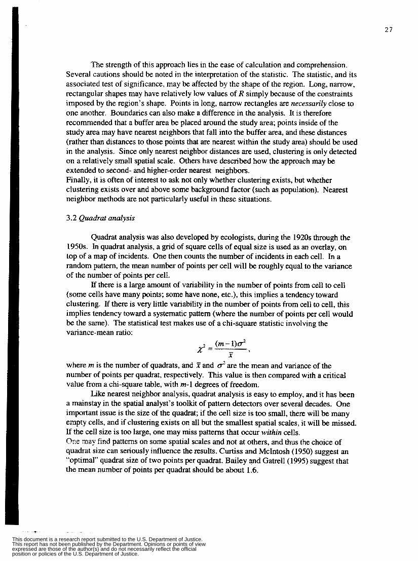
If there is a large amount of variability in the number of points from cell to cell
where m is the number of quadrats, and Z and o2 are the mean and variance of the number of points per quadrat, respectively. This value is then compared with a critical value from a chi-square table, with m-1 degrees of freedom.
a mainstay in the spatial analyst’s toolkit of pattern detectors over several decades. One important issue is the size of the quadrat; if the cell size is too small, there will be many empty cells, and if clustering exists on all but the smallest spatial scales, it will be missed. If the cell size is too large, one may miss patterns that occur within cells. One may find patterns on some spatial scales and not at others, and thus the choice of quadrat size can seriously influence the results. Curtiss and McIntosh (1950) suggest an “optimal” quadrat size of two points per quadrat. Bailey and Gatrell(1995) suggest that the mean number of points per quadrat should be about 1.6.
Like nearest neighbor analysis, quadrat analysis is easy to employ, and it has been
This document is a research report submitted to the U.S. Department of Justice.This report has not been published by the Department. Opinions or points of viewexpressed are those of the author(s) and do not necessarily reflect the officialposition or policies of the U.S. Department of Justice.
3.3 Moran’s I
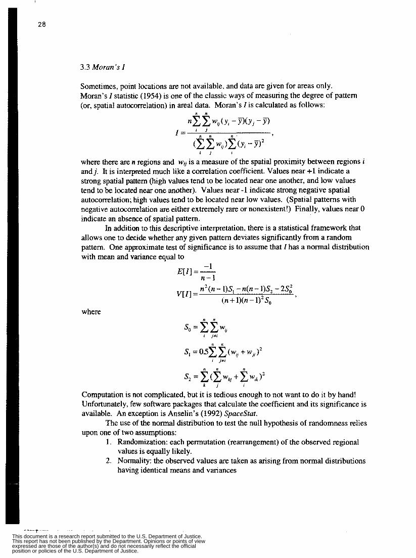
Sometimes, point locations are not available, and data are given for areas only. Moran’s I statistic (1954) is one of the classic ways of measuring the degree of pattern (or, spatial autocorrelation) in areal data. Moran’s I is calculated as follows:
n n
1 J t
where there are n regions and wo is a measure of the spatial proximity between regions i andj. It is interpreted much like a correlation coefficient. Values near +1 indicate a strong spatial pattern (high values tend to be located near one another, and low values tend to be located near one another). Values near -1 indicate strong negative spatial autocorrelation; high values tend to be located near low values. (Spatial patterns with negative autocorrelation are either extremely rare or nonexistent!) Finally, values near 0 indicate an absence of spatial pattern.
allows one to decide whether any given pattern deviates sigmficantly from a random pattern. One approximate test of significance is to assume that I has a normal distribution with mean and variance equal to
In addition to this descriptive interpretation, there is a statistical framework that
-1 n-1
E [ I ] = -
n’(n - I)S, - n(n - I)S, - 2s: V [ I ] = (n + l)(n - 1),S0
>
where
i j # i
n n
s, = 0 5 c (WG + Wj$ i j # i
Computation is not complicated, but it is tedious enough to not want to do it by hand! Unfortunately, few software packages that calculate the coefficient and its significance is available. An exception is Anselin’s (1992) Spacestat.
The use of the normal distribution to test the null hypothesis of randomness relies upon one of two assumptions:
1. Randomization: each permutation (rearrangement) of the observed regional values is equally likely.
2. Normality: the observed d u e s are taken as arising from normal distributions having identical means and variances
This document is a research report submitted to the U.S. Department of Justice.This report has not been published by the Department. Opinions or points of viewexpressed are those of the author(s) and do not necessarily reflect the officialposition or policies of the U.S. Department of Justice.

29
3.4 Oden ’s Ipop statistic
One of the characteristics of Moran’s I is that within-region variations can undermine the validity of the randomization or normality assumptions. For example, regions with small populations may be expected to exhibit more variability. Oden accounts for this within region variation explicitly by modifying I as follows:
where ri and pi are the observed and expected proportion of all cases falling in region i, respectively. Furthemore, there are m regions, n incidents, and a total base population of x. The overall prevalence rate is b =n/x. Also,
where
i j
i
Oden suggests that statistical significance be evaluated via a normal distribution, with mean and variance
-1 x - 1
EIIw] = -
2A2 -I- C12 - E A2x2 W W l = ,
where A is defined as above, and
m m
3.5 Tango’s Cc statistic
Tango (1995) has recently suggested the following global statistic to detect clusters:
In matrix form,
r This document is a research report submitted to the U.S. Department of Justice.This report has not been published by the Department. Opinions or points of viewexpressed are those of the author(s) and do not necessarily reflect the officialposition or policies of the U.S. Department of Justice.
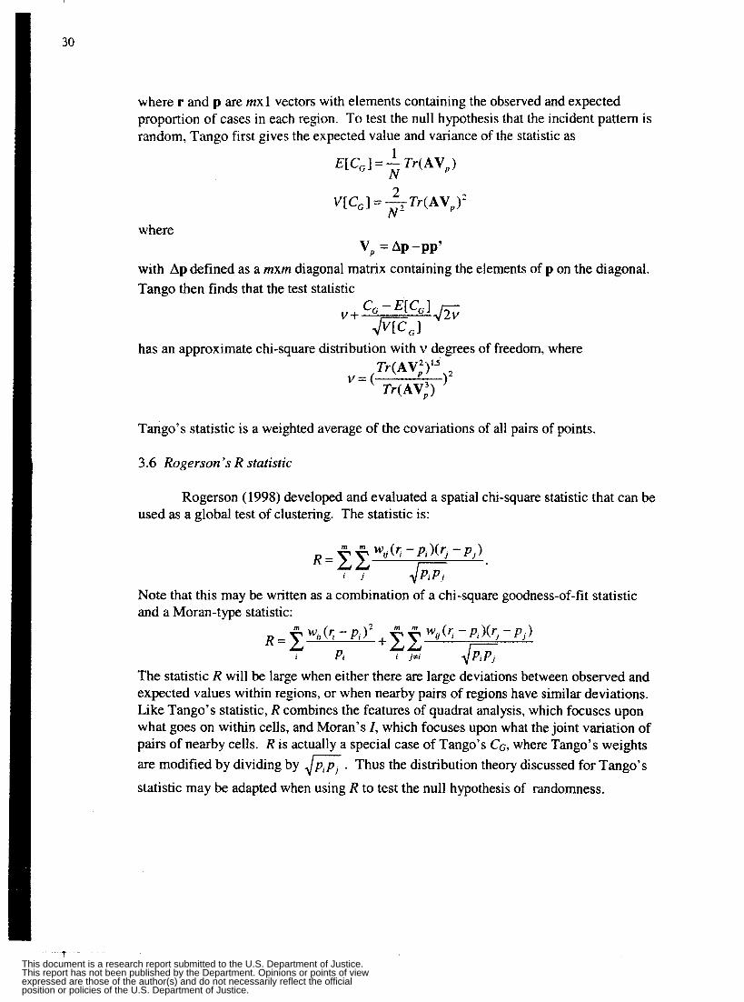
where r and p are nix1 vectors with elements containing the observed and expected proportion of cases in each region. To test the null hypothesis that the incident pattern is random, Tango first gives the expected value and variance of the statistic as
1 E[CG]=-T~(AV,) N n
where
with Ap defined as a mxm diagonal matrix containing the elements of p on the diagonal. Tango then finds that the test statistic
V, =Ap-pp’
has an approximate chi-square distribution with v degrees of freedom, where
V = ( )* Tr(AV;)’” Tr ( AV,) )
Tango’s statistic is a weighted average of the covariations of all pairs of points.
3.6 Rogerson ’s R statistic
Rogerson (1998) developed and evaluated a spatial chi-square statistic that can be used as a global test of clustering. The statistic is:
w I J ( ‘ ; - P J )
I J 4 G -
I Pt I J# I Jp,p,
Note that this may be written as a combination of a chi-square goodness-of-fit statistic and a Moran-type statistic:
Y,(< - P,I2 +g2 YJ‘; - P J q - P , ) R = Z
The statistic R will be large when either there are large deviations between observed and expected values within regions, or when nearby pairs of regions have similar deviations. Like Tango’s statistic, R combines the features of quadrat analysis, which focuses upon what goes on within cells, and Moran’s I , which focuses upon what the joint variation of pairs of nearby cells. R is actually a special case of Tango’s CG, where Tango’s weights are modified by dividing by f i . Thus the distribution theory discussed for Tango’s statistic may be adapted when using R to test the null hypothesis of randomness.
t This document is a research report submitted to the U.S. Department of Justice.This report has not been published by the Department. Opinions or points of viewexpressed are those of the author(s) and do not necessarily reflect the officialposition or policies of the U.S. Department of Justice.
4. Local Statistics
4. i Introduction
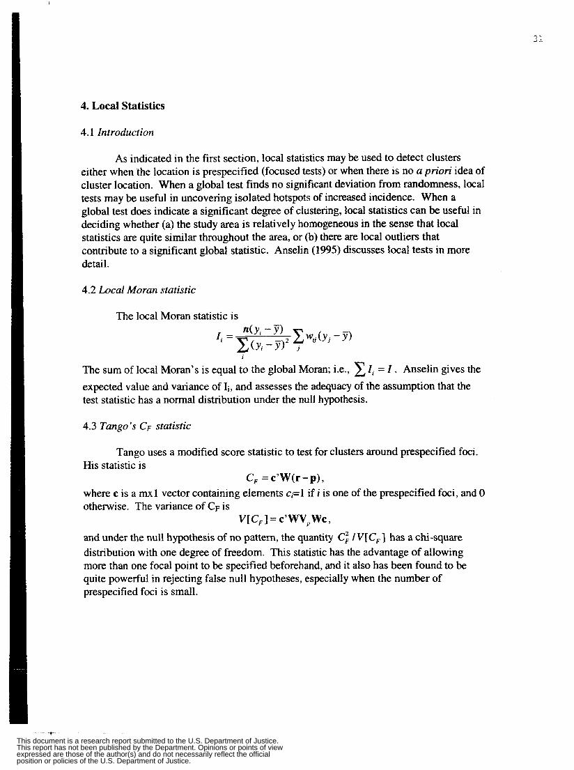
As indicated in the first section, local statistics may be used to detect clusters either when the location is prespecified (focused tests) or when there is no a priori idea of cluster location. When a global test finds no significant deviation from randomness, local tests may be useful in uncovering isolated hotspots of increased incidence. When a global test does indicate a significant degree of clustering, local statistics can be useful in deciding whether (a) the study area is relatively homogeneous in the sense that local statistics are quite similar throughout the area, or (b) there are local outliers that contribute to a significant global statistic. Anselin (1995) discusses local tests in more detail.
4.2 Local Moran statistic
The local Moran statistic is
i
The sum of local Moran’s is equal to the global Moran; Le., expected value and variance of Ii, and assesses the adequacy of the assumption that the test statistic has a normal distribution under the null hypothesis.
Z, = Z . Anseh gives the
4.3 Tango’s CF statistic
Tango uses a modified score statistic to test for clusters around prespecified foci. His statistic is
C, =c’W(r-p), where c is a mxl vector containing elements ci=i if i is one of the prespecified foci, and 0 otherwise. The variance of CF is
and under the null hypothesis of no pattern, the quantity C: / V[ C,] has a chi-square distribution with one degree of freedom. This statistic has the advantage of allowing more than one focal point to be specified beforehand, and it also has been found to be quite powerful in rejecting false null hypotheses, especially when the number of prespecified foci is small.
vrc, ] = c’ WV, wc ,
This document is a research report submitted to the U.S. Department of Justice.This report has not been published by the Department. Opinions or points of viewexpressed are those of the author(s) and do not necessarily reflect the officialposition or policies of the U.S. Department of Justice.
32
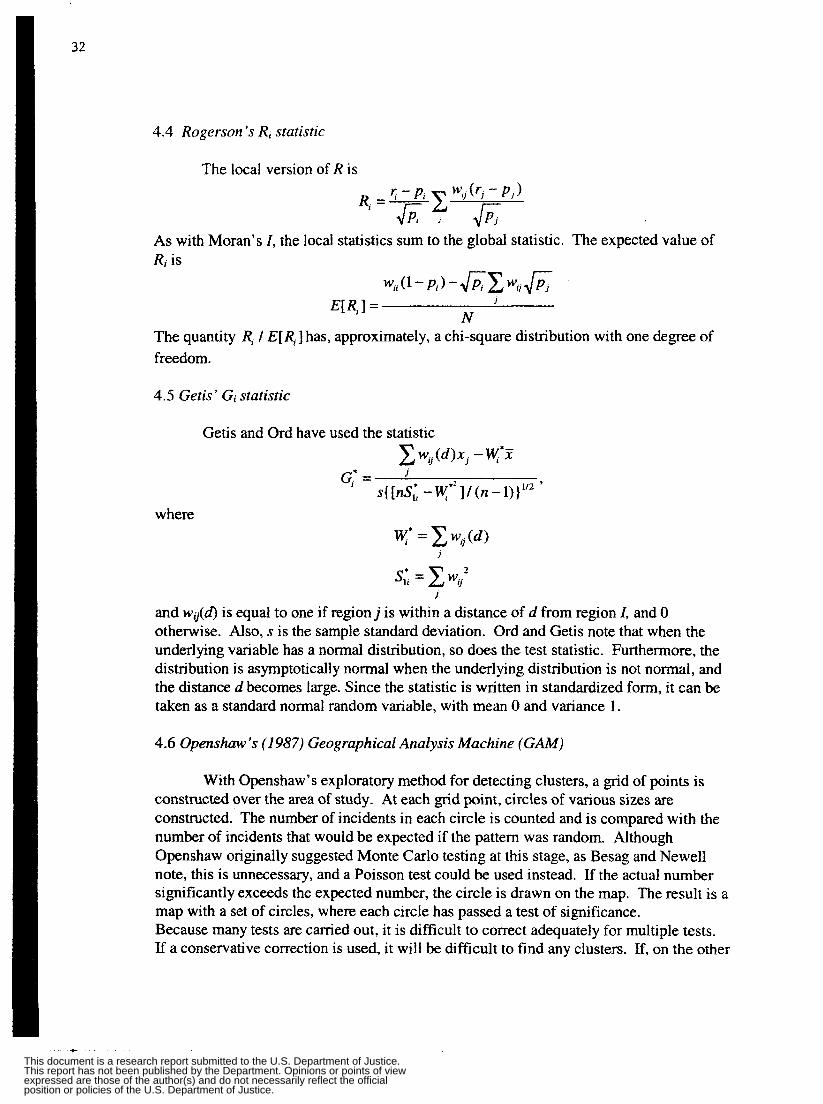
4.4 Roget-son’s R, statistic
The local version of R is
As with Moran’s I , the local statistics sum to the global statistic. The expected value of R, is
Wl, (1 - P, ) - Jptc Wq fi J
N EIRJ =
The quantity 8 / E[R,] has, approximately, a chi-square distribution with one degree of freedom.
4.5 Getis’ Gi statistic
Getis and Ord have used the statistic
where y* = c, w,(d)
i 2 sl; = wv
J
and wu(d) is equal to one if region j is within a distance of d from region I, and 0 otherwise. Also, s is the sample standard deviation. Ord and Getis note that when the underlying variable has a normal distribution, so does the test statistic. Furthermore, the distribution is asymptotically normal when the underlying distribution is not normal, and the distance d becomes large. Since the statistic is written in standardized form, it can be taken as a standard normal random variable, with mean 0 and variance 1.
4.6 Openshaw ’s (1 987) Geographical Analysis Machine (GAM)
With Openshaw’s exploratory method for detecting clusters, a grid of points is constructed over the area of study. At each gnd point, circles of various sizes are constructed. The number of incidents in each circle is counted and is compared with the number of incidents that wouid be expected if the pattern was random. Although Openshaw originally suggested Monte Carlo testing at this stage, as Besag and Newel1 note, this is unnecessary, and a Poisson test could be used instead. If the actual number significantly exceeds the expected number, the circle is drawn on the map. The result is a map with a set of circles, where each circle has passed a test of significance. Because many tests are carried out, it is difficult to correct adequately for multiple tests. If a conservative correction is used, it will be difficult to find any clusters. If, on the other
This document is a research report submitted to the U.S. Department of Justice.This report has not been published by the Department. Opinions or points of viewexpressed are those of the author(s) and do not necessarily reflect the officialposition or policies of the U.S. Department of Justice.
33
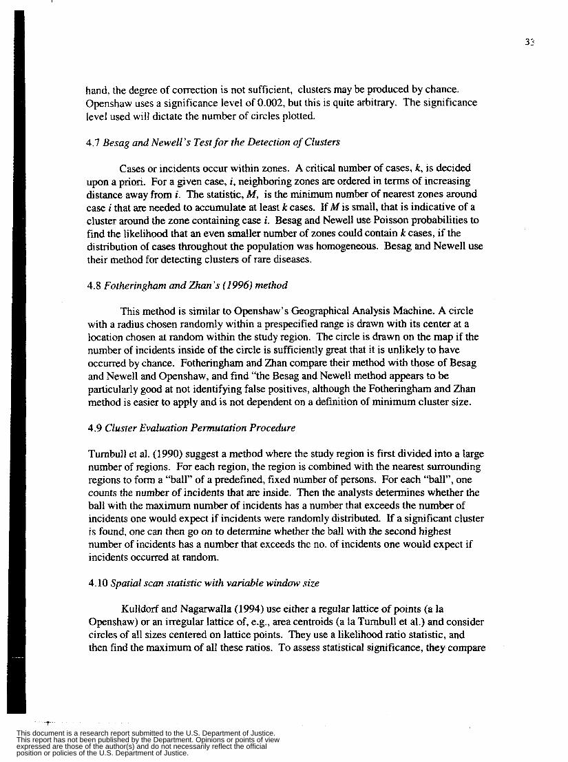
hand. the degree of correction is not sufficient, clusters may be produced by chance. Openshaw uses a significance level of 0.002, but this is quite arbitrary. The significance level used will dictate the number of circles plotted.
4.7 Besag and Newell’s Test for the Detection of Clusters
Cases or incidents occur within zones. A critical number of cases, k, is decided upon a priori. For a given case, i , neighboring zones are ordered in terms of increasing distance away from i. The statistic, M, is the minimum number of nearest zones around case i that are needed to accumulate at least k cases. If M is small, that is indicative of a cluster around the zone containing case i. Besag and Newell use Poisson probabilities to find the likelihood that an even smaller number of zones couId contain k cases, if the distribution of cases throughout the population was homogeneous. Besag and Newell use their method for detecting clusters of rare diseases.
4.8 Fotheringlzant and Zhan Is ( I 996) method
This method is similar to Openshaw’s Geographical Analysis Machine. A circle with a radius chosen randomly within a prespecified range is drawn with its center at a location chosen at random within the study region. The circle is drawn on the map if the number of incidents inside of the circle is sufficiently great that it is unlikely to have occurred by chance. Fotheringham and Zhan compare their method with those of Besag and Newell and Openshaw, and find “the Besag and Newell method appears to be particularly good at not identifying false positives, although the Fotheringham and Zhan method is easier to apply and is not dependent on a definition of minimum cluster size.
4.9 Cluster Evaluation Permutation Procedure
Tumbull et al. (1990) suggest a method where the study region is first divided into a large number of regions. For each region, the region is combined with the nearest surrounding regions to form a “ball” of a predefined, fixed number of persons. For each “ball”, one counts the number of incidents that are inside. Then the analysts determines whether the ball with the maximum number of incidents has a number that exceeds the number of incidents one would expect if incidents were randomly distributed. If a significant cluster is found, one can then go on to determine whether the ball with the second highest number of incidents has a number that exceeds the no. of incidents one would expect if incidents occurred at random.
4.10 Spatial scan statistic with variable window size
Kulldorf and Nagarwalla (1994) use either a regular lattice of points (a la Openshaw) or an irregular lattice of, e.g., area centroids (a la Turnbull et al.) and consider circles of all sizes centered on lattice points. They use a likelihood ratio statistic, and then find the maximum of all these ratios. To assess statistical significance, they compare
t This document is a research report submitted to the U.S. Department of Justice.This report has not been published by the Department. Opinions or points of viewexpressed are those of the author(s) and do not necessarily reflect the officialposition or policies of the U.S. Department of Justice.

34
the maximum among the likelihood ratios with the maximum obtained from a Monte Carlo simulation.
4.1 1 Openshaw ‘s Space-Time-Attribute Machiize (STAM)
attributes. The next step is to choose an observed data record. Then the size of geographic, temporal, and attribute search regions are chosen and one determines how many records lie within this tri-space region. Significance is assessed by using a Monte Carlo approach to determine the probability of observing that many records under the null hypothesis of no pattern. If the probability is sufficiently small, one saves the record. The idea is to examine all combinations of geographic, temporal, and attributes; those “search creatures” which do well reproduce, while those that do not find clusters die out. Thus an evolutionary element is embedded to speed up the search for interesting clusters.
Openshaw’s STAM begins by defining a study area across space, time, and
This document is a research report submitted to the U.S. Department of Justice.This report has not been published by the Department. Opinions or points of viewexpressed are those of the author(s) and do not necessarily reflect the officialposition or policies of the U.S. Department of Justice.
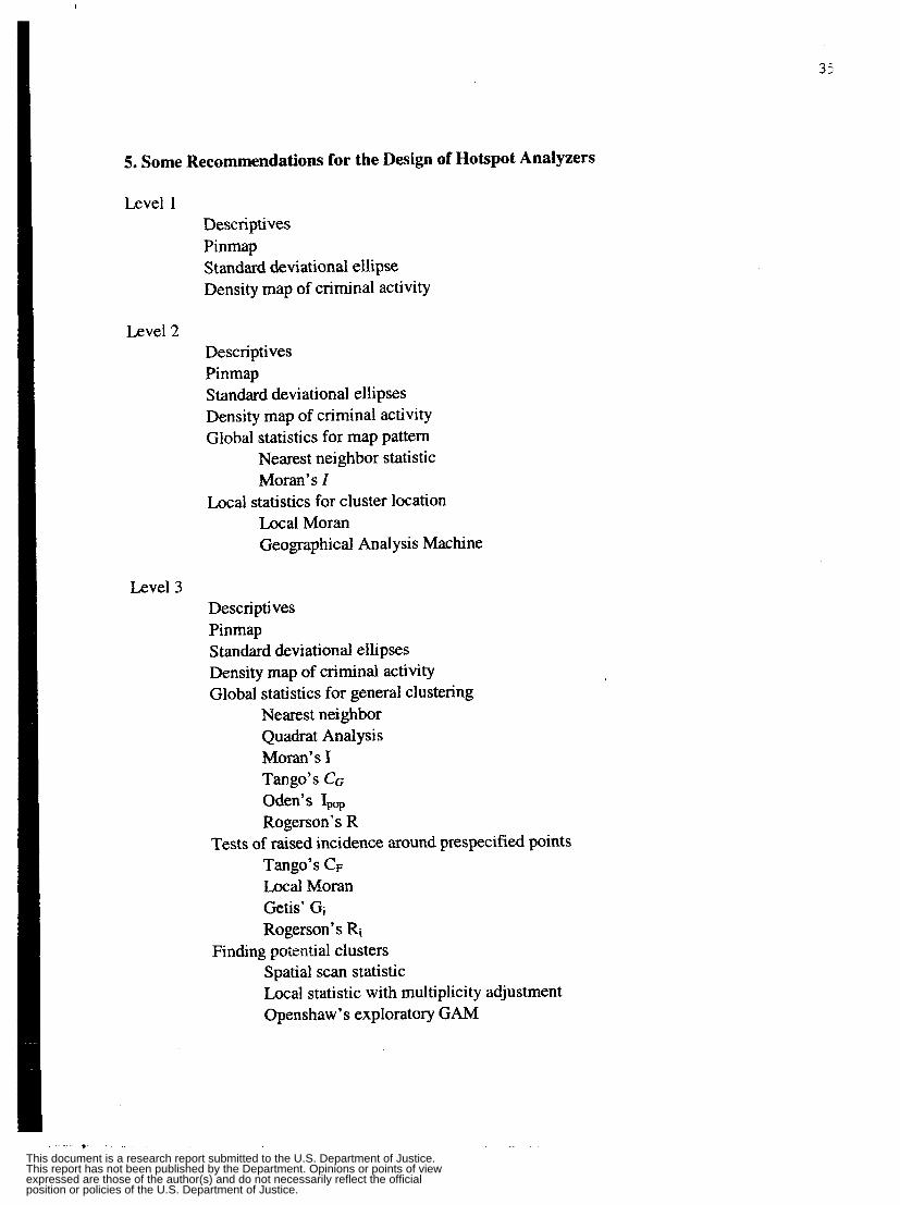
5. Some Recommendations for the Design of Hotspot Analyzers
Level 1 Descriptives Pinmap Standard deviational ellipse Density map of criminal activity
Level 2 Descriptives Pinmap Standard deviational ellipses Density map of criminal activity Global statistics for map pattern
Nearest neighbor statistic Moran’s I
Local Moran Geographical Analysis Machine
Local statistics for cluster location
Level 3 Descriptives Pinmap Standard deviational ellipses Density map of criminal activity Global statistics for general clustering
Nearest neighbor Quadrat Analysis Moran’s I
Oden’s Rogerson’s R
Tango’s CF Local Moran Getis’ Gi Rogerson’s Ri
Spatial scan statistic Local statistic with multiplicity adjustment Openshaw’s exploratory GAM
Tango’s C G
Tests of raised incidence around prespecified points
Findmg potential clusters
This document is a research report submitted to the U.S. Department of Justice.This report has not been published by the Department. Opinions or points of viewexpressed are those of the author(s) and do not necessarily reflect the officialposition or policies of the U.S. Department of Justice.
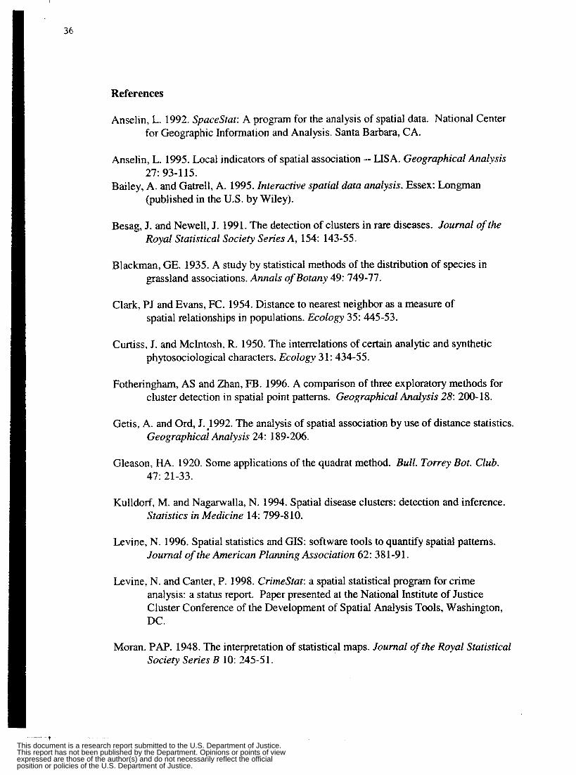
References
Anselin, L. 1992. SpaceStat: A program for the analysis of spatial data. National Center for Geographic Information and Analysis. Santa Barbara, CA.
Anselin, L. 1995. Local indicators of spatial association -- LISA. Geographical Analysis
Bailey, A. and Gatrell, A. 1995. Interactive spatial data analysis. Essex: Longman 27: 93-1 15.
(published in the U.S. by Wiley).
Besag, J. and Newell, J. 1991. The detection of clusters in rare diseases. Journal of the Royal Statistical Society Series A, 154: 143-55.
Blackman, GE. 1935. A study by statistical methods of the distribution of species in grassland associations. Annals of Botany 49: 749-77.
Clark, PJ and Evans, FC. 1954. Distance to nearest neighbor as a measure of spatial relationships in populations. Ecology 35: 445-53.
Curtiss, J. and McIntosh, R. 1950. The interrelations of certain analytic and synthetic phytosociological characters. Ecology 3 1: 434-55.
Fotheringham, AS and Zhan, FB. 1996. A comparison of three exploratory methods for cluster detection in spatial point patterns. Geographical Analysis 28: 200- 18.
Getis, A. and Ord, J. 1992. The analysis of spatial association by use of distance statistics. Geographicai Analysis 24: 189-206.
Gleason, HA. 1920. Some applications of the quadrat method. Bull. Torrey Bot. Club. 47: 21-33.
Kulldorf, M. and Nagarwalla, N. 1994. Spatial disease clusters: detection and inference. Statistics in Medicine 14: 799-810.
Levine, N. 1996. Spatial statistics and CIS: software tools to quantify spatial patterns. Journal of the American Planning Association 62: 38 1-91.
Levine, N. and Canter, P. 1998. Crimestat: a spatial statistical program for crime analysis: a status report. Paper presented at the National Institute of Justice Cluster Conference of the Development of Spatial Analysis Tools, Washington, DC.
Moran. PAP. 1948. The interpretation of statistical maps. Journal of the Royal Statistical Society Series B 10: 245-5 1.
t This document is a research report submitted to the U.S. Department of Justice.This report has not been published by the Department. Opinions or points of viewexpressed are those of the author(s) and do not necessarily reflect the officialposition or policies of the U.S. Department of Justice.
37
Oden, N. 1995. Adjusting Moran's I for population density. Statislics in Medicine 14: 17- 26.
Openshaw, S., Charlton, M., Wymer, C., and Craft, A. 1987. A mark 1 geographical analysis machine for the automated analysis of point data sets. Internarional Jmmai of Geogrqhiml Informution Systems 1: 335-58.
Openshaw, S. 1994. Two exploratory space-time-attribute pattern analysers relevant to GIs. In SptiaZamI&sis d G I S . Edited by AS Fotheringham and PA Rogerson, pp. 83-104.
Rogerson, P. 1998. A spdal version of the chi-square goodness-of-fit test and its application to tests for spatial clustering. In Spatial rndiing a& analysis: essays in honor of Jean Fueiinck. Edited by D. Griffith and C. Amrhein. Kfuwer- NijhofS 7 1-84.
Spatial and Temporal Analysis (STAC). Illinois Cnmhal Justice Information Authority.
Tango, T. 1995. A class of tests for detecting "general" and "fmsed" clustering of rare diseases. Statistics in Medicine 7: 649-60.
Turnbull, BW, Iwano, E3, Bumett, WS, Howe, HL, and Clark, LC. 1990. Monitoring for clusters of disease: application to leukemia incidence in upstate New York. American Jmmal of EpidemioZogy 13 2: S 13 6-43.
This document is a research report submitted to the U.S. Department of Justice.This report has not been published by the Department. Opinions or points of viewexpressed are those of the author(s) and do not necessarily reflect the officialposition or policies of the U.S. Department of Justice.

34
28 April 199%
MEMORANDUM
TO: Ezra Zubrow Lee Hunt
FROM: Hugh Calkins
SUBJEm Report and Recommendations on Choropleth mapping
Choropleth (or thematic) mapping is a basic tool for representing summay information by small geographic area. The main issues in preparing such maps are:
1.
2.
3.
4.
5 .
The se t ec t i~~ of the geographic unit and a collcern for substantid size differences between units - a large unit will give a biased appearance due to the size a l e - San Bemardin0 County is a good example. Howewer for our purposes, this may not be too much of a problem as police beats, blocks, and other urban units don't vary that much. The classificati.on methods used to determine the ranges for mapping - d e f W methods such as those in Arcview assume a normal (or near normal) disbibution for the data. Much of the urban data we will use will not have such a distribution. The defaults in Arcview are quintiles, equal intend, standard deviation and equal area. I suggest we add to this a capability to dtsptay the data in histogtam foxm and as a rank ordered array so users can see the pattern, and then provide a method to " p o i n t - d e on the histogram or array to specify the classifications: m g s . These seleCtions could
Normahaion of the data - on the basis of area, per capita or per household) - these options probably should be button driven. Color selection - we should design special color ramps for our purposes and give the user a little ore control over individual colors. There should be a s d INmber of defW color Sctremes for most users. Currently Arcview has too many choices of color ramp. Number of variables - we should allow for two variables to be displayed - one by color and the second by black pattern overlay.
then be W t Q d d & b into the legend editor. (see sample attached).
I would recommend three basic options for choropleth mapping:
1. The single button option From dropdown lists be able to select dataset (FI, Call-for-servk,ahe arrest or a socio-economic variable) and the spatial unit (beat, block, precinct, or census unit).
DeWts for color and classification (probably 5 classes, equal intmal)
t This document is a research report submitted to the U.S. Department of Justice.This report has not been published by the Department. Opinions or points of viewexpressed are those of the author(s) and do not necessarily reflect the officialposition or policies of the U.S. Department of Justice.

Display and label street centerlines and other significant features
2. Same as above but with greater user control over classification scheme and color - this will be much like the current version of AV.
3. An advanced capability incorporating the histogram and rank order array bctionality for the selection of classes.
This document is a research report submitted to the U.S. Department of Justice.This report has not been published by the Department. Opinions or points of viewexpressed are those of the author(s) and do not necessarily reflect the officialposition or policies of the U.S. Department of Justice.

Artificial Neural Networks in Forecasting Crime Emergence Author: Shoou-Jiun Wang
1. Crime Literature Review
Criminal activity is a space-time phenomenon which often doesn't match basic
assumptions of modem statistical theory. For example, its spatio-temporal distributions
appear to be chaotic or almost random and are usually non-linear and discontinuous
across space and time. Geographers and regional scientists have long realized that local
context and spatial heterogeneity are extremely important when forecasting space-time
phenomena (see for example Anselin, 1988), and have consequently devised a number of
ways in which to do so (see for example Cliff et al, 1975). Although with varying degree
of success, only few examples build successful models that employ spatio-temporal
forecasting techniques to crime patterns.
Geographic information systems have ability to plot the locations and frequencies
of the number of criminal activities. This ability produces high quality spatio-temporal
data sets and has resulted in tracking criminal activities successfully. Some police
agencies, for example, the Pittsburgh Bureau of Police, have begun to integrate
geographic information system with other sources of data such as 91 1 calls and police
records management systems.
Olligschlaeger (1997) introduces an early worming system that incorporates a
geographic information system previously developed to track criminal activity and a
relatively new technology, artificial neural networks, to predict the emergence of drug hot
spot areas. Artificial neural networks have many features which make them attractive for
spatio-temporal forecasting. First, they have a flexible and self-adaptive form which is
specific suitable to handle the nonlinear relationship between dependent and independent
variables. Second, A N N s do not require that parameters be initialized with regression
estimates, rather, the parameters are initialized randomly. To the best of our knowledge,
Olligschlaeger's research is the only artificial neutral network based spatio-temporal
forecasting models has been developed to date. Applying the algorithm to the data from
the Pittsburgh Bureau of Police, artificial neural network technique is shown to perform
better than traditional regression models do.
This document is a research report submitted to the U.S. Department of Justice.This report has not been published by the Department. Opinions or points of viewexpressed are those of the author(s) and do not necessarily reflect the officialposition or policies of the U.S. Department of Justice.

42
This new spatio-temporal forecasting methodology which combines artificial
neural networks and cellular automata with GIS-based data is referred as chaotic cellular
forecasting (CCF). One of the fundamental tenets of chaos theory is that although
chaotic systems seem to display totally random and unpredictable behavior they actually
follow strict mathematical rules which can be derive and studied (Pickover, 1990). This
character particularly fits our complicated crime activities. CCF uses a gradient descent
method to find the optimal neutron connection weights of artificial neural networks.
Most importantly, CCF has a nonlinear functional form commonly used in neural set
modeling, allowing for increased pattern recognition and accommodation of spatio-
temporal heterogeneity. The focus of this article is to describe how CCF was developed
and to explain the underlying theory behind neutral network. Next section is a literature
review on neural networks. Section three describes the two types of CFF algorithms, one
with temporally and spatially constant weights and the other with temporally constant but
spatially varying weights from input to hidden neutron, in detail. In section four,
advantages and disadvantages of neural networks are discussed and some possible further
studies are proposed. The final section provides some recommendations for the
development of chaotic cellular forecasting software.
2. Neural Networks Literature Review
Most commonly, there are three fundamental types of artificial neural networks:
supervised models, unsupervised or self-organizing models, and hybrid models.
Supervised models are by far most commonly applied. The spatially and temporally
constant weight type of CCF introduced in section 3 is a supervised model. Supervised
models, as we will see later, need target (correct) outputs as a criteria to adjust connection
weights between neutrons. In self-organizing model, there is no such need. Instead, the
network changes its internal connection strengths to recognize current patterns of inputs.
ANNs are also found in mixed environments which employ other technologies in
addition to neural models. The temporally constant but spatially varying type of CCF in
section 3 is a hybrid model.
Most important among artificial neural networks’ properties are ANN’S ability to
learn to identify complex patterns of information and to associate them with other
t This document is a research report submitted to the U.S. Department of Justice.This report has not been published by the Department. Opinions or points of viewexpressed are those of the author(s) and do not necessarily reflect the officialposition or policies of the U.S. Department of Justice.
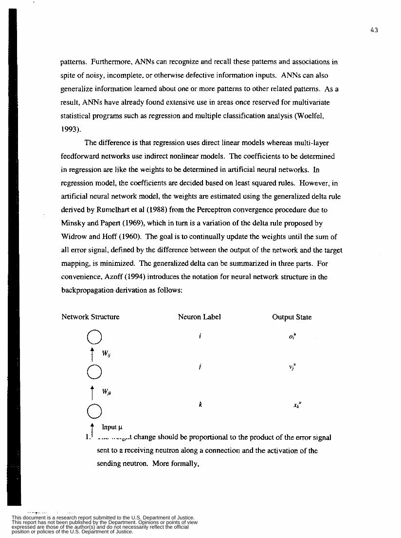
43
patterns. Furthermore, ANNs can recognize and recall these patterns and associations in
spite of noisy, incomplete, or otherwise defective information inputs. ANNs can also
generalize information learned about one or more patterns to other related patterns. As a
result, ANNs have already found extensive use in areas once reserved for multivariate
statistical programs such as regression and multiple classification analysis (Woelfel,
1 993).
The difference is that regression uses direct linear models whereas multi-layer
feedforward networks use indirect nonlinear models. The coefficients to be determined
in regression are like the weights to be determined in artificial neural networks. In
regression model, the coefficients are decided based on least squared rules. However, in
artificial neural network model, the weights are estimated using the generalized delta rule
derived by Rumelhart et al(1988) from the Perceptron convergence procedure due to
Minsky and Papert (1969), which in turn is a variation of the delta rule proposed by
Widrow and Hoff (1960). The goal is to continually update the weights until the sum of
all error signal, defined by the difference between the output of the network and the target
mapping, is minimized. The generalized delta can be summarized in three parts. For
convenience, Azoff (1994) introduces the notation for neural network structure in the
backpropagation derivation as follows:
Network Structure Neuron Label Output State
0 1 wij
0
0
1
i
k
0;
t InPUtCL 1. I .... .. -.es.t change should be proportional to the product of the error signal
sent to a receiving neutron along a connection and the activation of the
sending neutron. More formally,
This document is a research report submitted to the U.S. Department of Justice.This report has not been published by the Department. Opinions or points of viewexpressed are those of the author(s) and do not necessarily reflect the officialposition or policies of the U.S. Department of Justice.
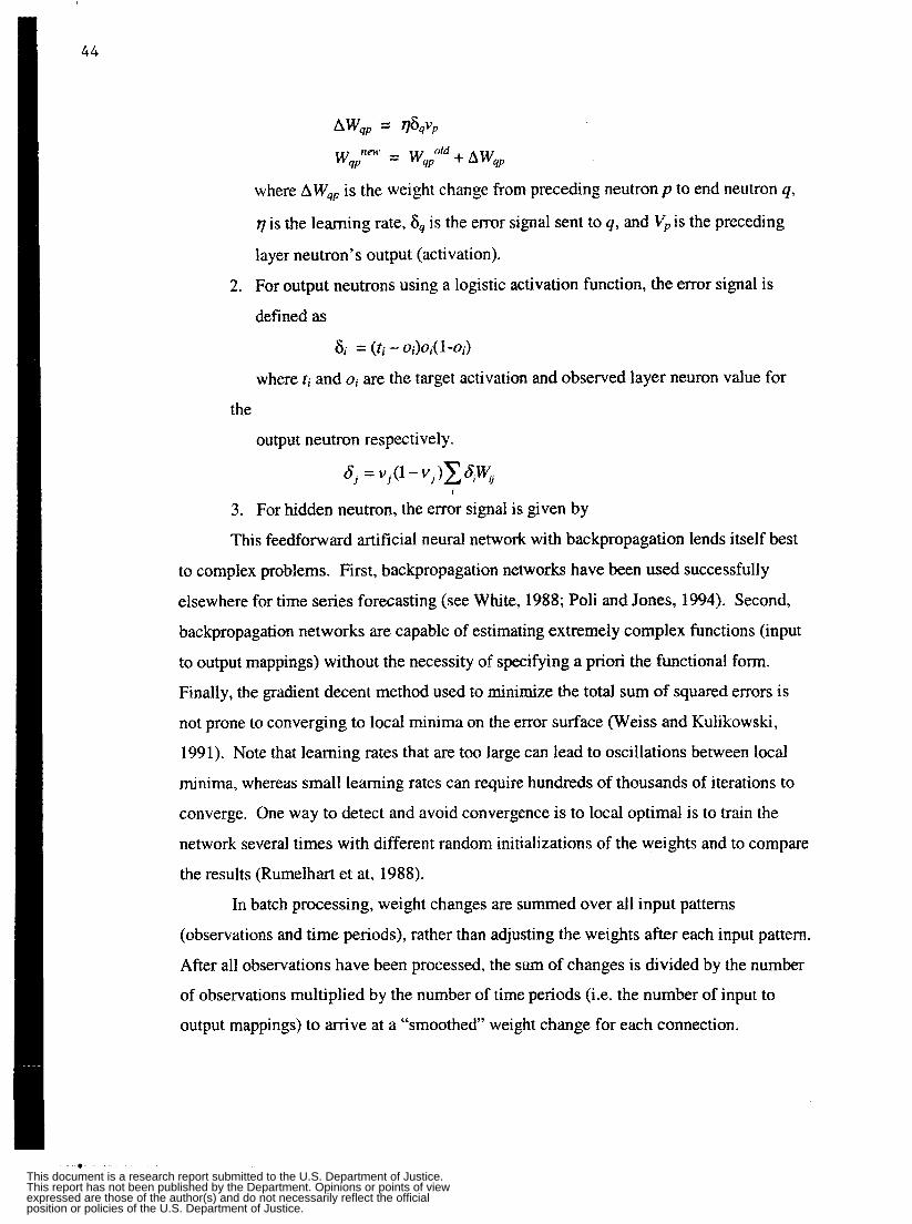
AWqp = M 9 V P
W q F = wq;ld 4- AWqp
where AW,, is the weight change from preceding neutron p to end neutron q,
q is the learning rate, S9 is the error signal sent to q, and V, is the preceding
layer neutron’s output (activation).
2. For output neutrons using a logistic activation function, the error signal is
defined as
St = (tj - oi)oi(l-oi)
where t, and ut are the target activation and observed layer neuron value for
the
output neutron respectively.
3. For hidden neutron, the error signal is given by
This feedforward artificial neural network with backpropagation lends itself best
to complex problems. First, backpropagation networks have been used successfully
elsewhere for time series forecasting (see White, 1988; Poli and Jones, 1994). Second,
backpropagation networks are capable of estimating extremely complex functions (input
to output mappings) without the necessity of specifying a priori the functional form.
Finally, the gradient decent method used to minimize the total sum of squared errors is
not prone to converging to local minima on the error surface (Weiss and Kulikowski,
1991). Note that learning rates that are too large can lead to oscillations between local
minima, whereas small learning rates can require hundreds of thousands of iterations to
converge. One way to detect and avoid convergence is to local optimal is to train the
network several times with different random initializations of the weights and to compare
the results (Rumelhart et at, 1988).
In batch processing, weight changes are summed over all input patterns
(observations and time periods), rather than adjusting the weights after each input pattern.
After all observations have been processed, the sum of changes is divided by the number
of observations multiplied by the number of time periods (Le. the number of input to
output mappings) to arrive at a “smoothed” weight change for each connection.
This document is a research report submitted to the U.S. Department of Justice.This report has not been published by the Department. Opinions or points of viewexpressed are those of the author(s) and do not necessarily reflect the officialposition or policies of the U.S. Department of Justice.
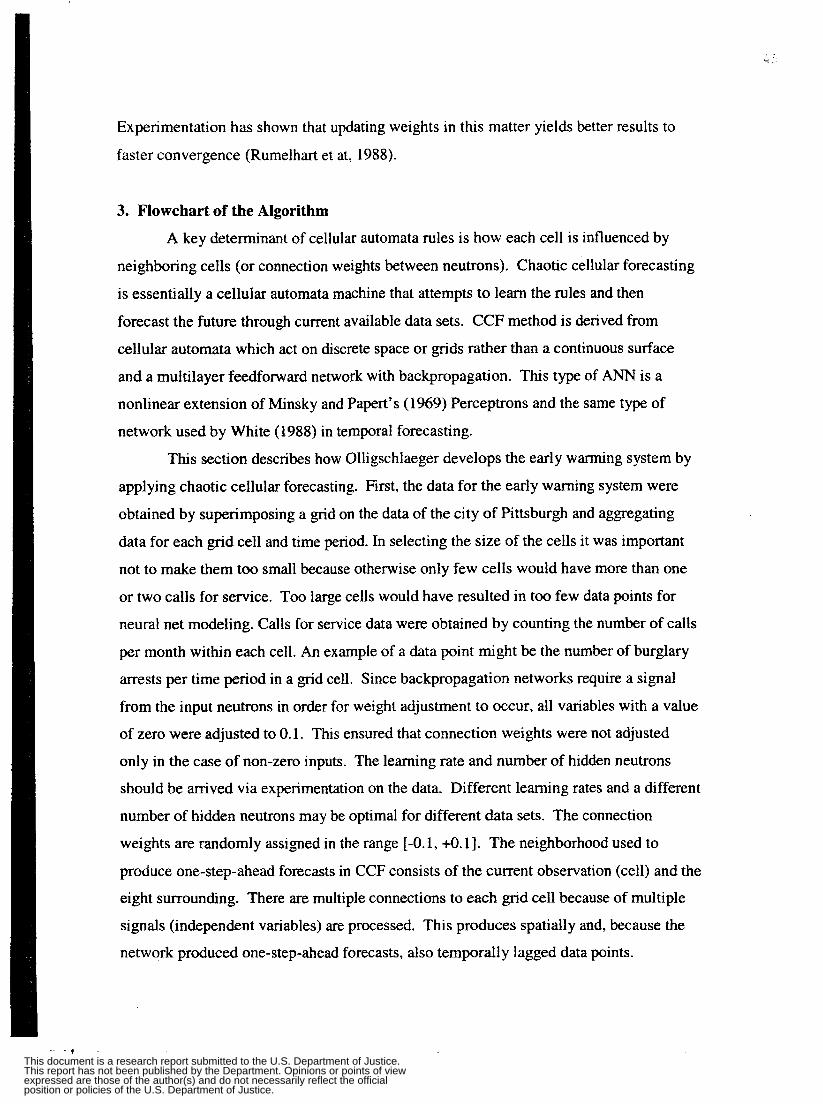
Experimentation has shown that updating weights in this matter yields better results to
faster convergence (Rumelhart et at, 1988).
3. flowchart of the Algorithm
A key determinant of cellular automata rules is how each cell is influenced by
neighboring cells (or connection weights between neutrons). Chaotic cellular forecasting
is essentially a cellular automata machine that attempts to learn the rules and then
forecast the future through current available data sets. CCF method is derived from
cellular automata which act on discrete space or gnds rather than a continuous surface
and a multilayer feedforward network with backpropagation. This type of ANN is a
nonlinear extension of Minsky and Papert’s (1969) Perceptrons and the same type of
network used by White (1988) in temporal forecasting.
This section describes how Olligschlaeger develops the early warming system by
applying chaotic cellular forecasting. First, the data for the early warning system were
obtained by superimposing a grid on the data of the city of Pittsburgh and aggregating
data for each grid cell and time period. In selecting the size of the cells it was important
not to make them too small because otherwise only few cells would have more than one
or two calls for service. Too large cells would have resulted in too few data points for
neural net modeling. Calls for service data were obtained by counting the number of calls
per month within each cell. An example of a data point might be the number of burglary
arrests per time period in a grid cell. Since backpropagation networks require a signal
from the input neutrons in order for weight adjustment to occur, all variables with a value
of zero were adjusted to 0.1. This ensured that connection weights were not adjusted
only in the case of non-zero inputs. The learning rate and number of hidden neutrons
should be arrived via experimentation on the data. Different learning rates and a different
number of hidden neutrons may be optimal for different data sets. The connection
weights are randomly assigned in the range [-0.1, +O. 11. The neighborhood used to
produce one-step-ahead forecasts in CCF consists of the current observation (cell) and the
eight surrounding. There are multiple connections to each grid cell because of multiple
signals (independent variables) are processed. This produces spatially and, because the
network produced one-step-ahead forecasts, also temporally lagged data points.
t
This document is a research report submitted to the U.S. Department of Justice.This report has not been published by the Department. Opinions or points of viewexpressed are those of the author(s) and do not necessarily reflect the officialposition or policies of the U.S. Department of Justice.
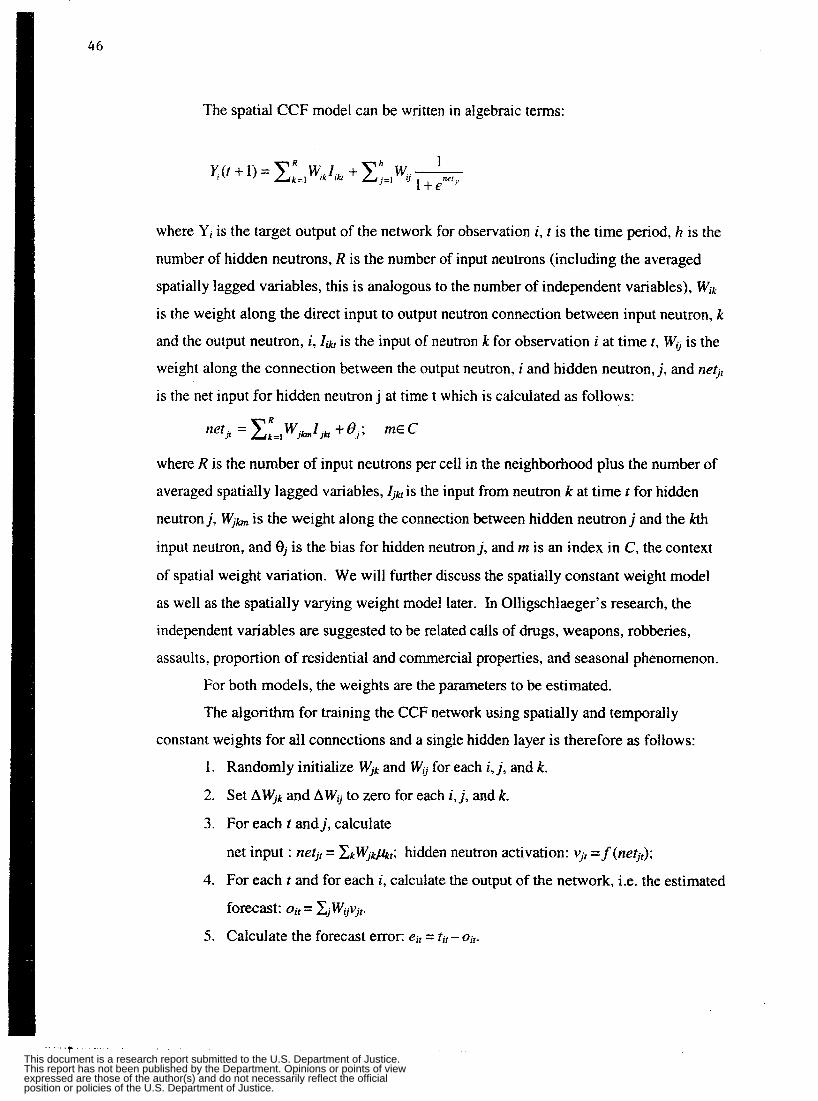
46
The spatial CCF model can be written in algebraic terms:
where Y, is the target output of the network for observation i, t is the time period, h is the
number of hidden neutrons, R is the number of input neutrons (including the averaged
spatially lagged variables, this is analogous to the number of independent variables), W,k
is the weight along the direct input to output neutron connection between input neutron, k
and the output neutron, i, Iib is the input of neutron k for observation i at time t , W, is the
weight along the connection between the output neutron, i and hidden neutron, j , and net,,
is the net input for hidden neutron j at time t which is calculated as follows: R
net,, = E,, wjh~,& + e,; mE c where R is the number of input neutrons per cell in the neighborhood plus the number of
averaged spatially lagged variables, Zjk is the input from neutron k at time t for hidden
neutron j, W j h is the weight along the connection between hidden neutron j and the kth
input neutron, and 0, is the bias for hidden neutron j , and m is an index in C, the context
of spatial weight variation. We will further discuss the spatially constant weight model
as well as the spatially varying weight model later. In Olligschlaeger's research, the
independent variables are suggested to be related calls of drugs, weapons, robberies,
assaults, proportion of residential and commercial properties, and seasonal phenomenon.
For both models, the weights are the parameters to be estimated.
The algorithm for training the CCF network using spatially and temporally
constant weights for all connections and a single hidden layer is therefore as follows:
I. Randomly initialize W,k and W;, for each i, j , and k.
2. Set A F k and AWQ to zero for each i , j , and k.
3. For each t andj, calculate
net input : netI, = & W j k h t ; hidden neutron activation: Vjr =f(netjr);
4. For each t and for each i, calculate the output of the network, i.e. the estimated
forecast: oit = &WljVjt.
5. Calculate the forecast error: e,, = r,, - oN-
This document is a research report submitted to the U.S. Department of Justice.This report has not been published by the Department. Opinions or points of viewexpressed are those of the author(s) and do not necessarily reflect the officialposition or policies of the U.S. Department of Justice.

47
6.
7.
8.
9.
For each connection (input to hidden and hidden to output) calculate the
weight change and add it to the sum of weight changes,AW, for that
connection over all forecasts.
Calculate the square forecast error and add to the sum of square forecast errors
e' = C, Zr e ir.
WjknPH = ykold + A W/(N*T), where N is the number of observations.
W,;'" = W$ld + AW/(G*T), where G is the number of gnd cells.
2
10. If the total sum of squared forecast errors in the current iteration is greater
than or equal to that of the previous iteration, stop. Otherwise, go to 3.
A second CCF algorithm relaxed the spatially constant weight assumption in that
each observation has its own unique set of input neutron connections and associated
weights for each cell in the neighborhood. However, the hidden to output neutron
weights are spatially constant. This produces a hybrid model that has the advantage of
some spatial variation in the weight structure but not too much to cause overfitting. The
algorithm for this hybrid CCF model, which assumes temporally constant but spatially
varying input to hidden neutron weights and a single layer of hidden neutrons is therefor:
1.
2.
3.
4.
5.
6.
7.
8.
Randomly initialize Wjh and W, for each i, j , k and n.
Set A W,h and A Wq to zero for each i, j , and k.
For each t andj, calculate net input : netjt = XkWjhNrn; hidden neutron
activation: vjr =f(netjr);
For each t and for each i, calculate the output of the network, i.e. the estimated
forecast: Oir = EjWovjr-
Calculate the forecast error: ei, = t i t- Oir.
For each connection (input to hidden and hidden to output) calculate the
weight change and add it to the sum of weight changes,AW, for that
connection and gnd cell n over all forecasts.
Calculate the square forecast error and add to the sum of square forecast errors
e2 = Xi xi e2it.
yhnew = W,hdd+AW/I'.
t This document is a research report submitted to the U.S. Department of Justice.This report has not been published by the Department. Opinions or points of viewexpressed are those of the author(s) and do not necessarily reflect the officialposition or policies of the U.S. Department of Justice.

9. Wtjny)I’ = W{ld + AW/(N*T), where N is the number of observations.
10. If the total sum of squared forecast errors in the current iteration is greater
than or equal to that of the previous iteration, stop. Otherwise, go to 3.
When calculating the input values of the neighborhood, a boundary problem
arises. Since backpropagation networks require that all input to output mappings have
the same number of input neutrons, CCF tackles this problem by assigning “imaginary”
neighbors to border cells. The inputs of the imaginary cells are set to zero.
4. Conclusion
A drawback of backpropagation networks is that they require a very large number
of observations for training. This problem is analogous to having too many parameters in
regression, resulting in not degrees of freedom. One solution to this problem is to
increase the number of observations using the capabilities of geographic information
systems . Further experimentation revealed that adding direct input to output connections to
the network architecture kept ovefitting in check, i.e., the network would generalize
better. In addition, it was found that averaging Spatially lagged variables from the
neighborhood of an observation rather than connecting each independent variable in each
neighboring grid to each hidden neutron reduced the number of connections and the
amount of overfitting. In other words, instead of nine sets of inputs, one from each
observation in the neighborhood, the architecture only had two sets: one from the current
observation, and one for the average spatially lagged independent variables of the eight
neighbors. In the Pittsburgh example, this adjustment speeds up the convergence four
times faster.
Another drawback of artificial neutral networks is the model is unable to represent
the results as an equation with parameters. Usually representing the relationship between
dependent and independent variables can be helpful in parameter sensitivity analysis.
An advantage of neural networks is the nonlinearity of transfer functions of the
neutrons and the multilayer structure of the network can ensure a good fitting for any
t This document is a research report submitted to the U.S. Department of Justice.This report has not been published by the Department. Opinions or points of viewexpressed are those of the author(s) and do not necessarily reflect the officialposition or policies of the U.S. Department of Justice.

I
49
functional form whatever. The other most advantage is no need for the analyst to
stipulate the functional form prior analysis, the ANN will find it automatically.
Three recommendations for further studies are made to conclude this section.
1 . In Olligschlaeger’s research, the spatial concern of an observation takes account
on its eight neighbors. If, in stead of using grid cells as neutrons, using police
patrol beats as neutrons, then the neighbors of the observation may not have equal
size. In this case, should we take the beats which connect to the observation as
spatially lagged variables? Or, should we define a neighborhood by a certain size
and take account all the beats within this neighborhood? A proposed suggestion
is introducing fussy logic in this point to decide the relationship between the
observation and its neighbors.
2. There are many ways in which backpropagation networks can be modified so that
they converge more quickly to a solution. An additional improvement would be
to employ genetic algorithms to develop self-optimizing architectures.
3. The number of hidden layers is a critical issue. For very complex input to output
mapping, two or more layers must be more appropriate to capture the nonlinear
relationship between input and output neturons.
This document is a research report submitted to the U.S. Department of Justice.This report has not been published by the Department. Opinions or points of viewexpressed are those of the author(s) and do not necessarily reflect the officialposition or policies of the U.S. Department of Justice.

50
5. Some Recommendations for the Design of Chaotic Cellular Forecasting
Level 1
D
0
0
0
Level 2
0
n
0
0
Level 3
P
O
0
0
Supervised model (spatially and temporally constant weights)
Use grid cells as neutrons
One hidden layer
Users choose number of hidden neutrons
Supervised model (spatially and temporally constant weights)
Users choose grid cells or police patrol beats as neutrons
Users choose number of hidden layers
Users choose number of hidden neutrons
Users choose supervised model (spatially and temporally constant weights) or
hybrid model (temporally constant but spatially varying weights)
Users choose grid cells or police patrol beats as neutrons
Users choose number of hidden layers
Users choose number of hidden neutrons
This document is a research report submitted to the U.S. Department of Justice.This report has not been published by the Department. Opinions or points of viewexpressed are those of the author(s) and do not necessarily reflect the officialposition or policies of the U.S. Department of Justice.
5 1
Reference: Anselin, L. ( 1988). Spatial Econometrics: Methods and Models, Dordrecht, Netherlands:
Kluwer.
Azoff, E.M. (1994). Neural Network Time Series Forecasting of Financial Markts. New York: John Wiley & Sons.
Cliff, A.D., P. Haggett, P., Basssett, K. and R. Davies. (1975). Elements of Spatial Stmcture. Cambridge, England: Cambridge University Press.
Minsky, M. and S. Papert. (1969). Perceptrons. Cambridge, PA: I”T Press.
Olligschlaeger, A. (1997). “Chaos Theory, Artificial Neural Networks and GIs-Based Data: Chaotic Cellular Forecasting and Application to the Prediction of Drug Related Call for Service Data.” Draft on October, Camegie Mellon University.
Pickover, C.A. (1990). Computers, Pattern, Chaos and Beauty. New York: St. Martin’s Press.
Poli, I. and R.D. Jones. (1994). “A Neutral Net Model for Prediction.” Journal ofthe American Statistical Association, 89: 1 17-2 1.
Rumelhart, D.E., G.E. Hinton, and R.J. Williams. (1988). “Learning Internal Representations by Error Propagatin.” In Rumelhart, D.E. and J.L. McCIelland. (eds.) Parallel Distributed Processing, Vol. 1, Cambridge, MA: MIT Press
Weiss, S.M. and C.A. Kulikowski. (1991). Computer Systems That Learn. Morgan Kaufman, San Mateo
White, H. (1988). ‘‘Economic Prediction Using Neural Networks: The Case of DBM Daily Stock Returns.” Proceedings of the lEEE International Conference on Neutral Networks, San Diego
Widrow, G and M.E. Hoff (1960). “Adaptive Switching Circuits.” Institute of Radio Engineers, Western Electronics Show and Convention
Woelfel, J. (1993). “Artificial Neural Networks in Policy Research: A Current Assessment.” Journal of Communication, 43: 63-80.
This document is a research report submitted to the U.S. Department of Justice.This report has not been published by the Department. Opinions or points of viewexpressed are those of the author(s) and do not necessarily reflect the officialposition or policies of the U.S. Department of Justice.

52
t
This document is a research report submitted to the U.S. Department of Justice.This report has not been published by the Department. Opinions or points of viewexpressed are those of the author(s) and do not necessarily reflect the officialposition or policies of the U.S. Department of Justice.

Pattern Analyses: Pattern Recognition Philip Mitchell
Pattern recognition, simply, is the attempt to isolate formalized pattern sets that are of interest or have similar associations. In the case of my research with patterns in crime data there are multitudes of associations that can be incorporated. As an increased number of data sets are added to support these associations the data set size starts to grow exponentially. When several data sets from different agencies are combined there are several conditions that disrupt or alter patterns. The most obvious is the use of differing basic indicators. If two data sets are used, each with a different identifier (Block 54) a matching pattern will be greatly understated.
evaluate violations associated with licensed liqueur establishments. The first data set is compiled from police reports where police consider liqueur establishments to mean bars, taverns and nightclubs. The second data set is compiled by the licensing agency, which includes all establishments that have a liqueur license to include grocery stores and restaurants. The correlation between the results of run one and two is only about 60%. The difference between the two sets is the definition of liqueur establishments. Even correcting for this difference in data sets may only raise the relationship up to 95%. The error dtfference between them has been greatly reduced.
that, although have associative coordinates are disassociate due to a physical barrier. An example is a depicted pattern area that is disassociated by a major highway running through the middle. If access between the subsets is restrictive the pattern is not associated as nearest neighbor. The pattern must therefore not have developed from spatial association but by some other association.
The degree to which a data set is organized and how spatial information is represented will effect the matching patterns. Layering data that is point specific, and clustered data represented as polygons will effect comparative associations. Examples of clustered precincts, demographic, socio-economic, ethnic orientation, gang, religious etc, compared to point specific violations is going to have effects on the resulting pattern.
Individuals will develop cognitive maps based on their mode of transportation. The activities and daily patterns of those using the metro system will differ greatly from those with privately owned vehicles. The degree to which these cognitive maps are similar will effect regional activities. Differing demographic groups within a regton will have varying cognitive maps that will be anchored to varying locations and time. An example of this is school students whose activities during school will be associated geographically with the school. In the evening the same individuals may be associated with a park or another hangout.
Fringe pattern analyses must also be considered. The interface of different spatial, demographic and political areas are bound to have effects due to their spatial associations. An example is the schoolyard where, for political (legal) implications, penalties for certain violations are maximized. This may result in an increase in criminal activities on the fringe area due not to the fringe area but as a result of the association.
Patterns within the data set are of primary concern to predicting criminal activity. There are several variables that hinder start forward ML pattern matching, such as spatial and temporal parameters within which the data exists. Further difficulties arise when considering geographically adjacent points that are not functionally adjacent.
only on the bases of space then change is not easily perceived. Consider crime in the city of
To illustrate the above I will refer to the example Block used. Two data sets are used to
Considerations must also be applied to spatial anomalies within the geographic region
Individuals within a region will have cognitive maps that will effect their activities.
Space should not be separated from time in the search for patterns. If the data is viewed
5 3
This document is a research report submitted to the U.S. Department of Justice.This report has not been published by the Department. Opinions or points of viewexpressed are those of the author(s) and do not necessarily reflect the officialposition or policies of the U.S. Department of Justice.

Pattern Analyses: Pattern Recognition Philip Mitchell
Buffalo over the past 200 years. Areas that have just recently experienced a plethora of crime will not greatly effect the 200 years of comparison. The same condition existed within the time frame of a day. A neighborhood that is, typically, crime free has a rash of petty crimes as the local school lets out. If this neighborhood’s crime is viewed within the time frame of the day it will still appear as a low crime area. Viewed within the time frame of an hour after school lets out it is a high crime area. Two dipolar conclusions.
temporally, occurring within a time frame such as day, evening and night. Seasons and weather will also have a patterning effect. In this case patterns develop within a short predictable period. Other non-obvious conditions such as school districts, places of employment, etc. can also act as an anchoring point for associative patterns to develop around.
Temporal patterns exist within a particular day within a year. Typically there is a correlation between Christmas Eve and Christmas with certain crimes (domestic disputes). It would be of greater use to compare the crime statistics for the last 5 years on Christmas Eve and Christmas then to look at the 5 days prior to Christmas. It might also be useful to compare Christmas Holiday incidents with its associated year’s crime to other Christmas holidays and their yearly statistics.
the city of Buffalo during known dates than to be able to quickly isolate those dates from the data set would also be useful.
Patterns can also develop in association to night and day. Although crime statistics might change in relation to the time of day they may fit within the temporal pattern set by sunset.
Pattern recognition is also hindered by temporal variability. Patterns may be isolated
Patterns for individuals can also be enhanced. If it were known that a suspect was within
Conclusion
and time are not a continual to which criminals feel obliged to adhere. Patterns must be searched for which have various cogrutive temporal associations. Space
The complete spatial randomness (CSR) after Diggle (1983) exists if the points that were generated are subject to the following two rules:
1. each location in the study area has an equal chance of receiving a point (uniformity); and
2. the selection of a location for a point is in no way influenced by the selection or location of any other point, (independence).
t This document is a research report submitted to the U.S. Department of Justice.This report has not been published by the Department. Opinions or points of viewexpressed are those of the author(s) and do not necessarily reflect the officialposition or policies of the U.S. Department of Justice.
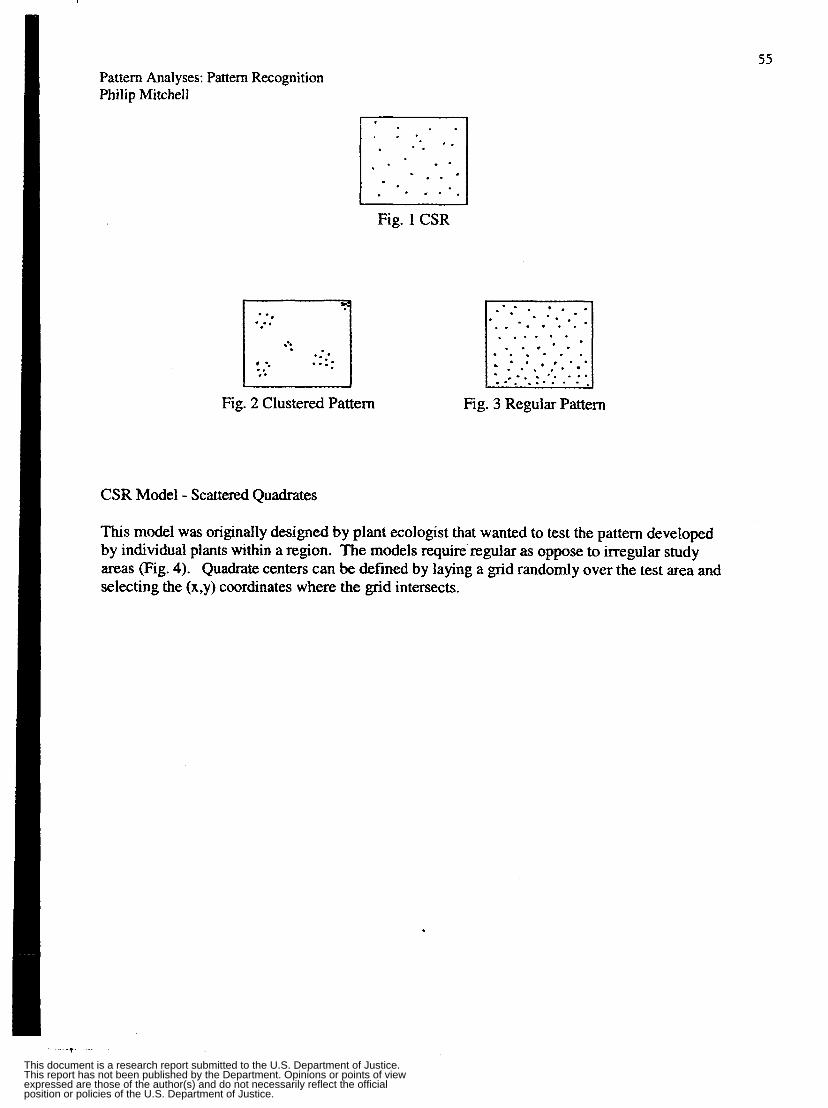
55 Pattern Analyses: Pattern Recognition Philip Mitchell
i-;1 .
*. ...e .. ..
. . a a .
. . . . . . - . . . * . * .
Fig. 2 Clustered Pattern
Fig. 1 CSR
I*;--.*:* .. ,;:*..: :I . . . . . . . . . . . . - . . , , . . . . . . . - * I . . .. ... ... ..... . .
Fig. 3 Regular Pattern
CSR Model - Scattered Quadrates
This model was originally designed by plant ecologist that wanted to test the pattern developed by individual plants within a region. The models require regular as oppose to irregular study areas (Fig. 4). Quadrate centers can be defined by laying a grid randomly over the test area and selecting the (x,y) coordinates where the grid intersects.
t
This document is a research report submitted to the U.S. Department of Justice.This report has not been published by the Department. Opinions or points of viewexpressed are those of the author(s) and do not necessarily reflect the officialposition or policies of the U.S. Department of Justice.
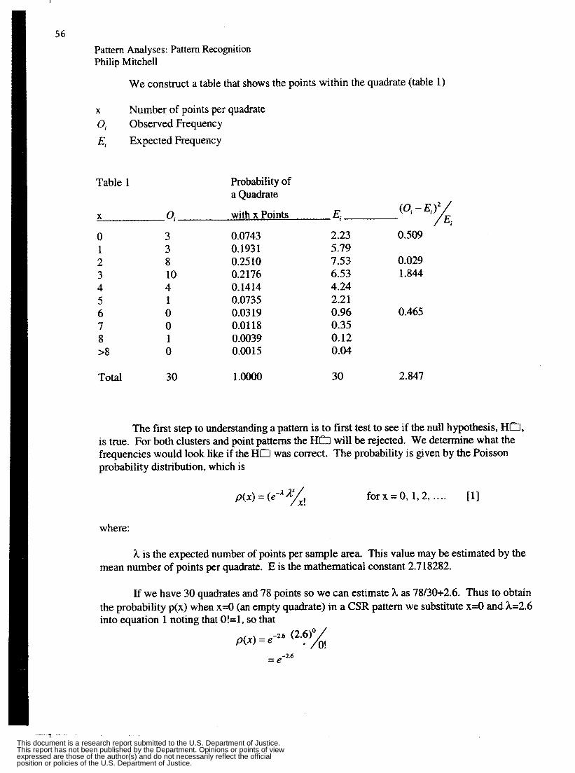
56
Pattern Analyses: Pattern Recognition Philip Mitchell
We construct a table that shows the points within the quadrate (table 1)
Number of points per quadrate X
0, Observed Frequency E, Expected Frequency
Table 1 Probability of a Quadrate with x Points Ei (0, - E , ) Z ,
X 0, 0 3 0.0743 2.23 0.509 1 3 0.1931 5.79 2 8 0.25 10 7.53 0.029 3 10 0.2 176 6.53 1.844 4 4 0.1414 4.24 5 1 0.0735 2.21 6 0 0.03 19 0.96 0.465 7 0 0.01 18 0.35 8 1 0.0039 0.12 >8 0 0.0015 0.04
Total 30 1 .m 30 2.847
The first step to understanding a pattern is to first test to see if the null hypothesis, HD, is true. For both clusters and point patterns the H B will be rejected. We determine what the frequencies would look like if the H D was correct. The probability is given by the Poisson probability distribution, which is
P(X) = (e-* y! for x = 0, 1,2, .... [I1
where:
h is the expected number of points per sample area. This value may be estimated by the mean number of points per quadrate. E is the mathematical constant 2.7 18282.
If we have 30 quadrates and 78 points so we can estimate h as 78/30+2.6. Thus to obtain the probability p(x) when x=O (an empty quadrate) in a CSR pattern we substitute x=O and h=2.6 into equation 1 noting that 0!=1, so that
P ( 4 = e -2.6 ( 2 . 6 ) x
-26 = e
This document is a research report submitted to the U.S. Department of Justice.This report has not been published by the Department. Opinions or points of viewexpressed are those of the author(s) and do not necessarily reflect the officialposition or policies of the U.S. Department of Justice.

Pattern Analyses: Pattern Recognition Philip Mitchell
=0.0743 For x= 1
= 0.1931
For x=2
=0.2510
Since the probability must sum to one the value of p(x>8) can be calculated from equation 2.
The test of the H D is accomplished by comparing the expected frequency against the obtained frequency.
131
Where: Oi Ei K
Observed Frequency in the ith category Expected Frequency in the ith category is the number of categories
The minimum value of k is an argued point but it should not be less then 5 per category.
Column 5 of table 2 is the values as calculated by equation 3.
Points can be examined under two different views: the dispersion of points in and area or the arrangement of points in relation to each other.
?
This document is a research report submitted to the U.S. Department of Justice.This report has not been published by the Department. Opinions or points of viewexpressed are those of the author(s) and do not necessarily reflect the officialposition or policies of the U.S. Department of Justice.
58 Pattern Analyses: Pattern Recognition Philip Mitchell
In the above example we tested the H, . In the event that we found the HkY to be true we would not be able to tell whether the pattern was a cluster or regular. Using the information from the table we can run a test of the H , to delineate between the two.
n is the number of quadrates fx is the observed frequency of x
In a Poisson probability distribution the value of h and V are expected to be equal. If h is greater then V. If V is less then h it indicates that each quadrate has an equal number of points. If there is clustering then V is greater then h.
An alternative equation is to use the chi-square test.
Nearest Neighbor Analyses in 2 dimensions
i=1
and obtaining the mean nearest neighbor distance
where n is the number of sampled points.
Clark and Evans (1954) equation shows the expected mean average of nearest neighbor distance, E(d , ) , for a random sample of points from a CSR pattern is approximated by the equation
E(di) = 0.54yN A is the area N points in the pattern
This document is a research report submitted to the U.S. Department of Justice.This report has not been published by the Department. Opinions or points of viewexpressed are those of the author(s) and do not necessarily reflect the officialposition or policies of the U.S. Department of Justice.
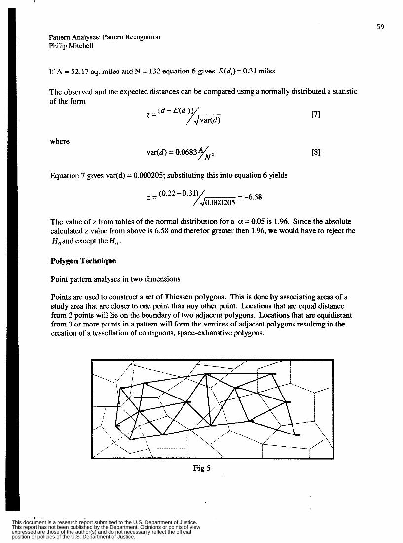
59
Pattern Analyses: Pattern Recognition Philip Mitchell
If A = 52.17 sq. miles and N = 132 equation 6 gives E(d j )= 0.31 mifes
The observed and the expected distances can be compared using a normally distributed z statistic of the form
where var(d) = 0.0683 yNz
Equation 7 gives v&d) = 0.000205; substituting this into equation 6 yields
z = (0.22 - 0 . 3 ~ 0 ~ 0 0 0 2 0 5 = -6.58
The value of z from tables of the normal distribution for a a = 0.05 is 1.96. Since the absolute calculated z value from above is 6.58 and therefor greater then 1.96, we would have to reject the H , and except the H, .
Polygon Technique
Point pattern analyses in two dimensions
Points are used to construct a set of Thiessen polygons. This is done by associating areas of a study area that are closer to one point than any other point. Locations that are equal distance from 2 points will lie on the boundary of two adjacent polygons. Locations that are equidistant from 3 or more points in a pattern will form the vertices of adjacent polygons resulting in the creation of a tessellation of contiguous, space-exhaustive polygons.
Fig 5
t This document is a research report submitted to the U.S. Department of Justice.This report has not been published by the Department. Opinions or points of viewexpressed are those of the author(s) and do not necessarily reflect the officialposition or policies of the U.S. Department of Justice.

60 Pattern Analyses: pattern Recognition Philip Mitchell
Using the Thiessen polygons for orientation another contiguous, space-exhaustive tessellation is produced known as the Delaunay triangulation. This is accomplished by joining points which share the Thiessen polygon edges.
Although there are several properties of these triangles that can be evaluated the most obvious is the size of the angles. The smallest angle can be quickly determined, which of course can not be greater then 60 degrees. Mardia et a1 (77) have developed probabilities for obtaining minimum angles less then or equal to some value of x, for Delaunay triangulation’s associated with a CSR pattern. This probability, P(x), is given by
P(x) = 1 + ‘/n7G[(6x - 2n)cos2x - sin 2x - sin 4x1 IS]
Values in one degree increments of P(x) for equation 8 can be compared to table 4.3
The test involves generating the Delaunay triangulation & identifying the minimum angles in the pattern at a specified interval of x, To avoid edge effect we restrict triangles that are produced by boundaries. The observed frequencies are cumulated and F(x) is calculated by dividing each of the observed cumulative frequencies by the sum of the frequencies.
P(x) for a CSR pattern can be obtained from column 3 of table 4.3 and shown in column 5 of table 4.4.
The absolute difference between values of F(x) and P(x) can be compared using a one-sample Kolmogorov-Smirnov (K-S) test.
The largest number in column 6 of table 4.4 determines the test statistic, Dmax, which is compared with the appropriate value from statistical tables of critical values. If the patterns Dmax is 0.0680, whereas the critical value is 0.2178 we can’t reject the Ha of the CSR pattern.
If the Ha is rejected the triangle angles can still be evaluated tentatively. A pattern that is arranged perfectly regularly will result in Thiessen polygons that are all regular hexagons, All of the angles within the pattern will measure 60 degrees. In the real world if a large number of minimum angles are approximately 60 degrees a regular pattern exists. Similarly, if a grid pattern exists a large percentage of the minimum angles will be approximately 45 degrees.
Table 4.3 Probability that the Minimum Angle of a Triangle in a Deaunay Triangulation for a Random Point Pattern is Less then or Equal to a Given Value of x.
Cluster Process Model quoted from Ripley’s Spatial Statistics p164-165
A Poisson cluster process is defined by taking a Poisson process of intensity a of parent points and centering on each parent an independent daughter process of object. The observed process may be either parents plus daughters of just all daughter objects. We will assume the latter. Another way to view this mechanism is to have an infinite set of independent identically
?
This document is a research report submitted to the U.S. Department of Justice.This report has not been published by the Department. Opinions or points of viewexpressed are those of the author(s) and do not necessarily reflect the officialposition or policies of the U.S. Department of Justice.
61
Pattern Analyses: Pattern Recognition Philip Mitchell
distributed processes, to use a Poisson process to select a translation for each, and then to add up the objects in all the translated processes. This suggests a modification in which we choose a Poisson process of rigid motion, thereby giving each daughter process an independent uniformly distributed rotation. We will assume that each daughter process contains a finite number of objects. The cluster process will always be homogeneous, but will only be isotropic if the daughter process is isotropic or if the daughters are given an additional rotation The most useful subclass of Poisson cluster processes is Neyman-Scott processes, for which each daughter object is independently distributed around the parent. Then if n is the (random) number of objects in the daughter process,
K ( t ) = m2 = E(n(n - 1))f(t)/A2 [8.16]
[8.17]
where all expectations are over n, f is the cumulative distribution function of the distance between two daughters with the same parent, and g(x,t) is the probability that a daughter point does not fall within distance t of x.
Equation (8.16) can be derived from interpretation (1) of K(t). The pairs of points can come either from dlfferent clusters giving the first term by the independence of clusters, or from the same cluster. If there are n objects in that cluster, the expected number of pairs not more then t apart is n(n- l)f(t), from which is derived the second term. Note that K(t) -nt@ is an increase function and that we can infer an estimate of f(t), and hence the cluster size, from O(t). Formula (8.17) is a special case of (9.10). Consider the N parent points within a bounded set D. For large D of area A.
1-p(t)=P(no daughter with parent in D is within t of the origin)
= CC'*~(CX A)" {no daughter within t / parent in D) }" /N!
= exp- = A(1- 'P (no daughter within t / parent in D))
= exp- = Ail - jDE(g(x , t )"d(x ) lA)
using the independence of the daughters and the uniform distribution of parent in D. Letting D increase gives (8.17).
Of course the parent process need not be Poisson; it could itself be a cluster process, giving rise to processes with a (finite) hierarchy of clusters. Another possibility is to take a regular process of parents to avoid the overlapping of clusters.
This document is a research report submitted to the U.S. Department of Justice.This report has not been published by the Department. Opinions or points of viewexpressed are those of the author(s) and do not necessarily reflect the officialposition or policies of the U.S. Department of Justice.
6 2
Pattern Analyses: Pattern Recognition Philip Mitchell
References
Block, C. R. 1997 The Geoarchive: An Information Foundation for Community Policing, In
Weisburd, D. and T. McEwen (editors), Crime Mapping and Crime Prevention, Criminal
Justice Press, Monsey, NY.
Boots, B. N. and A. Getis
1988 Point Pattern Analysis, Sage Publications, Beverly Hills.
Goos, C. and J. Hartmanis (editors)
1985 Functional Promumnine; Lanmages and Computer Architecture, Nancy, France,
September 1985, L. Augustsson, Compiling Pattern Matching, p368-38 1 , Beltz
Offsetdruck, Springer-Verlag, New York.
Goos, G., J. Hartmanis, and J. van Leeuwen (editors)
1996 Partial Evaluation, Sestoft, Peter, ML Pattern Match Compilation and Partial
Evaluation, P446-464, Springer-Verlag, Berlin.
Mather, P. M.
1993 Geoaaphic Information Handling - Research and Applications, John Wiley &
Sons, NY.
Milner, Robin, Mads Tofte
1991 Commentary on Standard ML, MIT Press, Cambridge, Massachusetts.
Milner, Robin, Mads Tofte, and Robert Harper
1990 The Definition of Standard ML, MIT Press, Cambridge, Massachusetts.
This document is a research report submitted to the U.S. Department of Justice.This report has not been published by the Department. Opinions or points of viewexpressed are those of the author(s) and do not necessarily reflect the officialposition or policies of the U.S. Department of Justice.
63 Pattern Analyses: Pattern Recognition Philip Mitchell
Olligschlaeger, Andreas M.
1997 October Draft - Chaos Theorv, Artificial Neural Networks and GIS-Based Data:
Chaotic Cellular Forecasting; and Application to the Prediction of Drug Related Call for
Service Data, H. John Heinz III School of Public Policy and Management, Carnegie
Mellon University, PA.
Ripley, B. D.
1981 Spatial Statistics, John Wiley & Sons, NY.
t
This document is a research report submitted to the U.S. Department of Justice.This report has not been published by the Department. Opinions or points of viewexpressed are those of the author(s) and do not necessarily reflect the officialposition or policies of the U.S. Department of Justice.

t This document is a research report submitted to the U.S. Department of Justice.This report has not been published by the Department. Opinions or points of viewexpressed are those of the author(s) and do not necessarily reflect the officialposition or policies of the U.S. Department of Justice.

65
Patrol Car Allocation Tool (PCAT)
Christopher M. Rump Dept. of Industrial Engineering
University at Buffalo Buffalo, NY 14260-2050 crump8ene.buffalo .edu
Note: Programmer notes appear in italics.
Notation: K = number of call priority classes J = number of geographic jurisdictions in the allocation T = number of time blocks (hours, shifts, days, etc.) in the week R = number of patrol car hours to be allocated each week
A j = size (square miles) of geographic jurisdiction j , j=I,.. .,J v j t = average response velocity (miles per hour) in geographic jurisdiction j during
time block t; j=1, ..., J, t=l, ..., T
for priority class k in jurisdiction j during time block t; k=l,.. .TK, j=l,., .,I, t=I,. ..,T 2-kjt = calls for service (CFS) arrival rate (calls received per hour)
p-kjt = service rate for priority class k in jurisdiction j during time block t = I/(averuge service time - dispatch until close - in hours)
r j t = number of patrol cars to allocate to jurisdiction j during time block t s j t = eflective number of patrol cars allocated to jurisdiction j during time block t
(after accounting for time spent unavailable for calls)
1 Choose method for patrol car allocation:
0 Hazard Formula - allocation by call-for-service (CFS) rates (default) Data required: CFS rates User level: elementary
0 Workload Formula - allocation by officer utilization Data required: CFS rates, service (travel + on-scene) times User level: intermediate
0 Queueing Formula - allocation based on response times, probability of queueing, queue size, etc. Data required: CFS rates, service (travel + on-scene) times, response velocities User level: advanced 1
2 How many weekly patrol-car hours are available for allocation? (= R) (Calculatefrom data m via user input?: eg., for 2-man cars, car hours = man hours/2,
I 07/12/99 9:18 AM
T
This document is a research report submitted to the U.S. Department of Justice.This report has not been published by the Department. Opinions or points of viewexpressed are those of the author(s) and do not necessarily reflect the officialposition or policies of the U.S. Department of Justice.
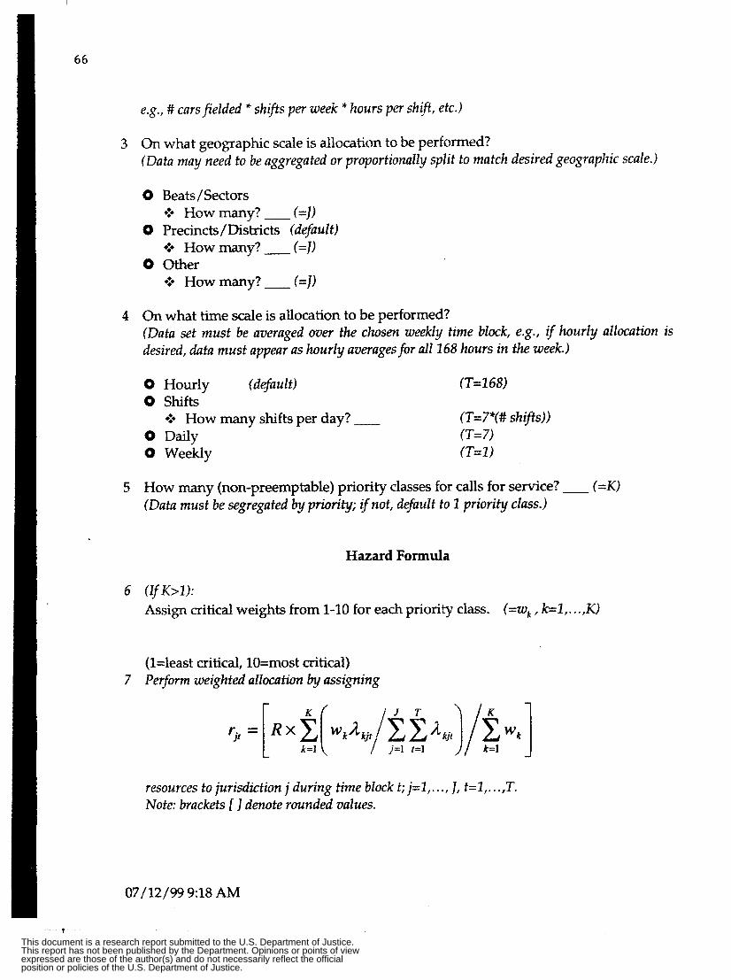
66
e.g., # carsfielded * sh$s per week * hours per shqt, etc.)
3 On what geographic scale is allocation to be performed? (Data may need to be aggregated or proportionally split to match desired geographic scale.)
0 Beats/Sectors
0 Precincts/Districts (default) *:* How many? - (=J)
0 Other *:* How many? - (=J)
*:* How m y ? - (=J)
4 On what time scale is allocation to be performed? (Data set must be averaged over the chosen weekly time block, e.g., if hourly allocation is desired, data must appear as hourly averages for all 268 hours in the week.)
0 Hourly (dgault) (T=268) 0 Shifts
0 Daily (T=7) 0 Weekly (T=l )
e.* How many shifts per day? ____ (T=7*(# shifts))
5 How many (non-preemptable) priority classes for calls for service? - (=K) (Data must be segregated by priority; if not, dqault to 1 priority class.)
Hazard Formula
6 (ZfK>I): Assign critical weights from 1-10 for each priority class. (=wk , k=l,. . .,IC)
(l=least critical, lO=most critical) 7 Perfom weighted allocation by assigning
resources to jurisdiction j during time block t; j=1,. . ., 3; t=Z,. . .,T. Note: brackets 11 denote rounded values.
07/12/99 998 AM
This document is a research report submitted to the U.S. Department of Justice.This report has not been published by the Department. Opinions or points of viewexpressed are those of the author(s) and do not necessarily reflect the officialposition or policies of the U.S. Department of Justice.
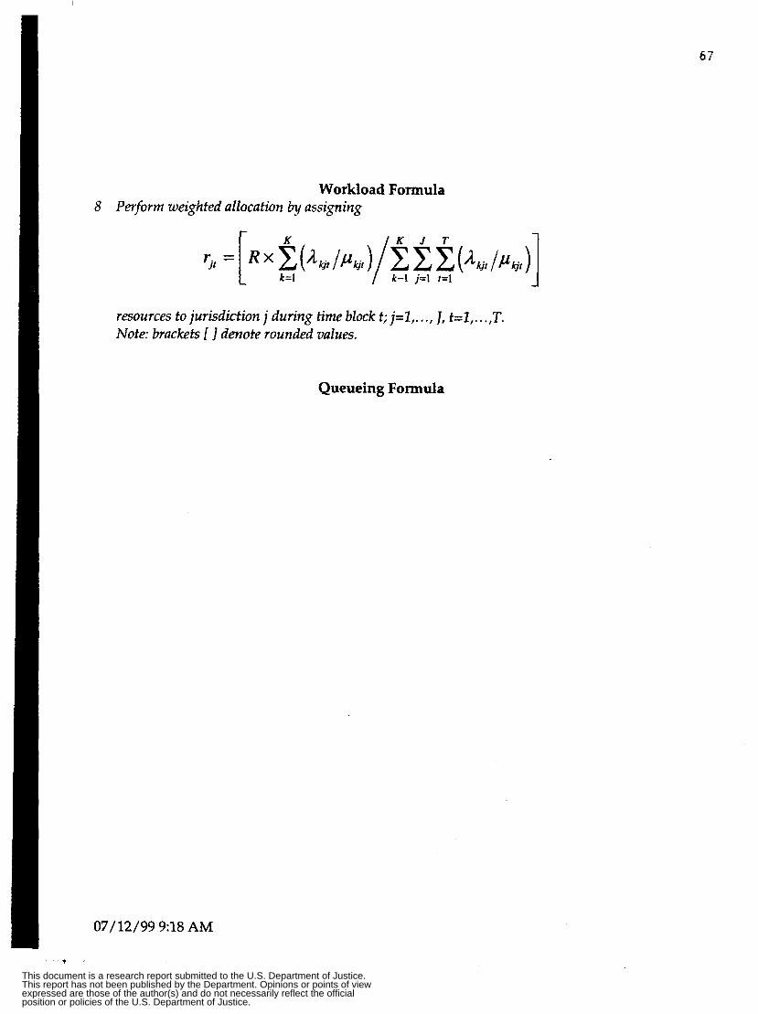
63
Workload Formula 8 Perform weighted allocation by assigning
resources tu jurisdiction j during time block t; j=1,. . ., J, t=Z,. . .,T. Note: brackets f 3 denote rounded values.
Queueing Formula
07/12/99 9:18 AM i This document is a research report submitted to the U.S. Department of Justice.This report has not been published by the Department. Opinions or points of viewexpressed are those of the author(s) and do not necessarily reflect the officialposition or policies of the U.S. Department of Justice.
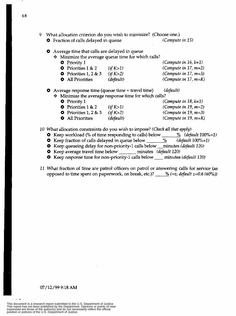
I
68
9 What allocation criterion do you wish to minimize? (Choose one.) 0 Fraction of calls delayed in queue (Compute in 15)
0 Average time that calls are delayed in queue *’* Minimize the average queue time for which calls?
0 Priority 1 (Compute in 16, k=Z) 0 Priorities 1 & 2 (Compute in 17, m=2) 0 Priorities 1,2 & 3 ( i fK>2) (Compute in 17, m=3) 0 All Priorities (default) (Compute in 17, m=K)
(if K>l)
0 Average response time (queue time + travel time) (default)
0 Priority1 (Compute in 18, k=I) 0 Priorities 1 & 2 ( i f K > l ) (Compute in 19, m=2) 0 Priorities 1,2 & 3 (i fK>2) (Compute in 19, m=3) 0 All Priorities (default) (Compute in 19, m=K)
*:* Minimize the average response time for which calls?
10 What allocation constraints do you wish to impose? (Check all that apply) 0 Keep workload (“/o of time responding to calls) below 0 Keep fraction of calls delayed in queue below 0 Keep queueing delay for non-priority-1 calls below -minutes (default 120) 0 Keep average travel time below 0 Keep response time for non-priority-1 calls below - minutes (dqauZt 120)
% (default 100%=2) YO (default 100%=2)
minutes (default 120)
11 What fraction of time are patrol officers on patrol or answering calls for service (as YO (=z; default z=0.6 (60%)) opposed to time spent on paperwork, on break, etc.)?
07/12/99 9:18 AM
t
This document is a research report submitted to the U.S. Department of Justice.This report has not been published by the Department. Opinions or points of viewexpressed are those of the author(s) and do not necessarily reflect the officialposition or policies of the U.S. Department of Justice.
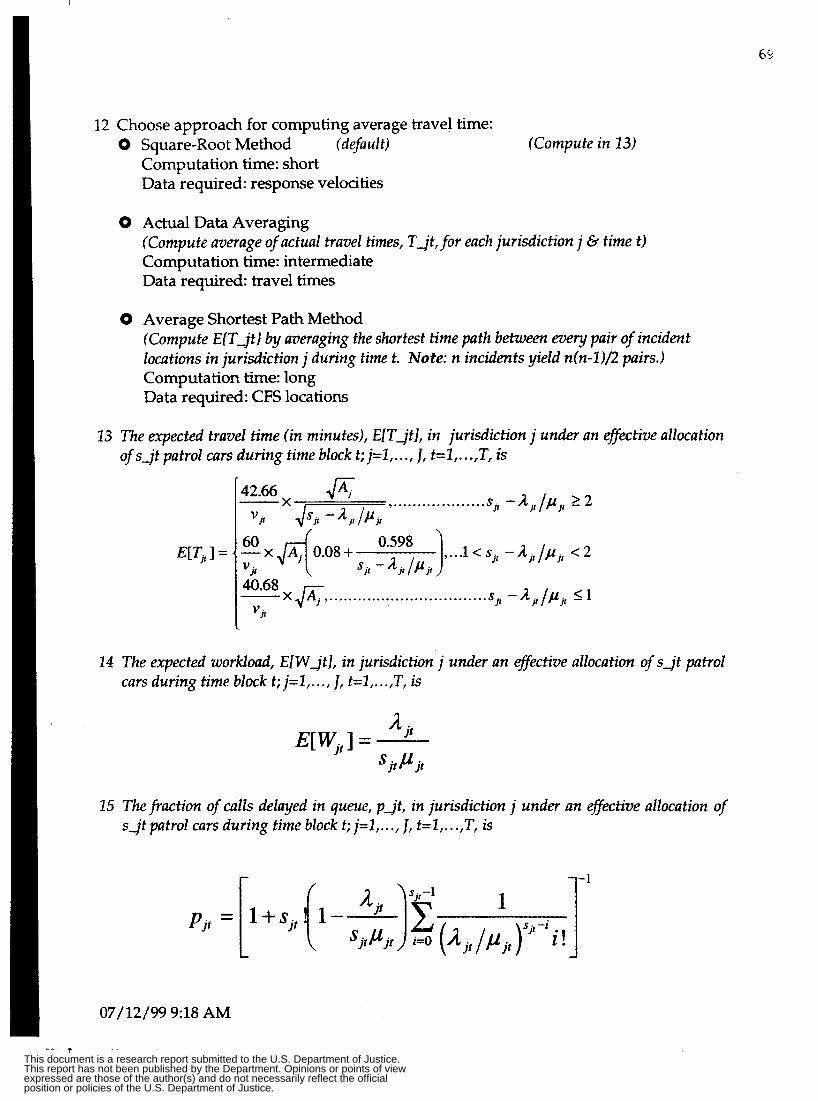
12 Choose approach for computing average travel time: 0 Square-Root Method (default) (Compute in 231
Computation time: short Data required: response velocities
0 Actual Data Averaging (Compute average of actual travel times, T i t , for each jurisdiction j 6, time t ) Computation time: intermediate Data required: travel times
0 Average Shortest Path Method (Compute E(TJt) by averaging the shortest time path between eve y pair of incident locations in jurisdiction j during time t. Note: n incidents yield n(n-1)/2 pairs.) Computation time: long Data required: CFS locations
13 The expected travel time (in minutes), E[T& in jurisdiction j under an gective allocation of s j t patrol cars during time block t; j=I ,.. . , J, t=2 ,.. .,T, is
,......"........... sjt -'jt /Pjt '2 42.66 JAj
vjt d m
The expected workload, E[W$], in jurisdiction j under an gective alloca,sm o f s j t patrol cars during time block t; j=1,. . ., 1, t=l,. ..,T, is
A . S j t p j t
E[Wjf ] = It
15 Thefraction of calls delayed in queue, p j t , in jurisdiction j under an effective allocation of s j t patrol cars during time block t; j=l,.. . , J, t=I ,. . . ,T, is
07/12/99 9:18 AM
t This document is a research report submitted to the U.S. Department of Justice.This report has not been published by the Department. Opinions or points of viewexpressed are those of the author(s) and do not necessarily reflect the officialposition or policies of the U.S. Department of Justice.
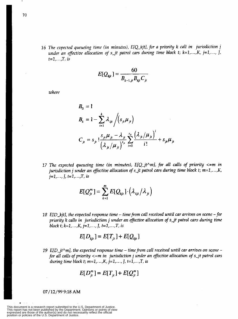
70
26 The cxpected queueing time (in minutes), EfQ-kjtf, for a priority k call in jurisdiction j under un efective allocation of s j t patrol curs during time block t; k=2, ..., K, j=2,..., J, t=Z,. . .,T, is
60 B . C E@, 3 =
' k - l , j t kjt J!
where
Bo = 1
17 The expected queueing time (in minutes), EIQjtAml, for all calls of priority c=m in jurisdiction j under an effective allocafion of s j t patrol cars during time block t; m=l,. . .,K, j=2 ,..., J, t=l, ..., T, is
m
k=l
28 E[D-kjtf, the expected response time - timefrom calE received until car arrives on scene -for priority k calls in jurisdiction j under an efectiue allocation of sjf patrol cars during time block t; k=I ,..., K, j=Z ,..., J, t=l, ..., T, is
29 E[DjtAm], the expected response time - timefrom call received until car arrives on scene - for all calls of priority <=m in jurisdiction j under an effective allocation ofs-jt patrol cars during time block t; m=2,. . .,K, j=1,. , ., J, t=I,. . .,T, is
E[DY] Jt = E[T. I t ] + E[QJT]
07/12/99 9:18 AM
This document is a research report submitted to the U.S. Department of Justice.This report has not been published by the Department. Opinions or points of viewexpressed are those of the author(s) and do not necessarily reflect the officialposition or policies of the U.S. Department of Justice.
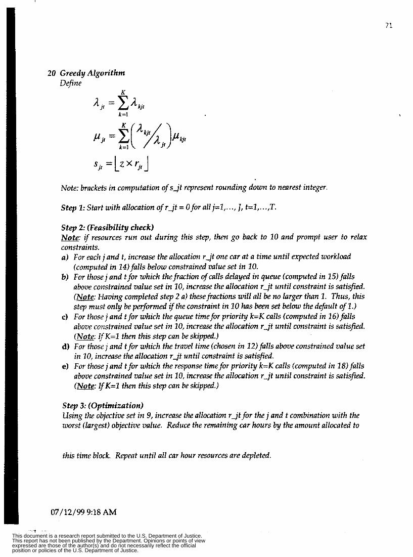
20 Greedy Algorithm Define
K
k =1
k=l
Note: brackets in computation of s j t represent rounding down to nearest integer.
Step 1: Start with allocation of r j t = 0 for all j=I , ..., J, t=l, ..., T.
S t e p 2: (Feasrln’liiy check) Note: if resources run out during this step, then go back to 10 and prompt user to relax constraints. a) For each j and t, increase the allocation r j t one car at a time until expected workload
b) For those j and t for which thefraction ofcalls delayed in queue (computed in 15) falls (computed in 14) falls below constrained value set in 10.
above constrained value set in 10, increase the allocation r j t until constraint is satisfied. (Note: Having completed step 2 a) thesefiactions will all be no larger than 1. Thus, this step must only be perfmmed if the constraint in 10 has been set below the default of 1 .)
c) For those i and t for which the queue time for priority k=K calls (computed in 16) falls above cozzstrained value set in 20, increase the allocation r j t until constraint is satisfied. (Note: IfK=1 then this step can be skipped.)
d) For those j and t for which the travel time (chosen in 12) falls above constrained value set in IO, increase the allocation r j t until constraint is satisfied.
e) For those j and t for which the response time for priority k=K calls (computed in 18) falls above constrained value set in 10, increase the allocation r j t until constraint is satisfied. (Note: I f K=l then this step can be skipped.)
S t e p 3: (Optimization) Using the objective set in 9, increase the allocation r j t for the j and t combination with the worst (largest) objective value. Reduce the remaining car hours by the amount allocated to
this time block. Repeat until all car hour resources are depleted.
07/12/99 9:18 AM
7 2
t
? This document is a research report submitted to the U.S. Department of Justice.This report has not been published by the Department. Opinions or points of viewexpressed are those of the author(s) and do not necessarily reflect the officialposition or policies of the U.S. Department of Justice.

?
This document is a research report submitted to the U.S. Department of Justice.This report has not been published by the Department. Opinions or points of viewexpressed are those of the author(s) and do not necessarily reflect the officialposition or policies of the U.S. Department of Justice.

Precinct Design Optimization Tool (PDOT)
Christopher M. Rump Dept. of Industrial Engineering
University at Buffalo
crump8eng.buff alo.edu Buffalo, NY 14260-2050 .
Note: Programmer notes appear in italics.
Notation: K = number of call priority classes J = number ofgeographic jurisdictions T = number of time blocks (hours, shifts, days, etc.) in the week R = number of patrol car hours to be allocated each week
A j = size (square miles) of geographic jurisdiction j , j=l,. . .,J v j t = average response velocity (miles per hour) in jurisdiction j during time block t;
j=1,. . .,J, t=l,. . .,T
for priority class k in jurisdiction j during time block t; k=I,. . .,K, j=1, ..., 1, t=I,.. .,T A-kjt = calls for seraice (CFS) arrival rate (calls received per hour)
p-kjt = service rate for priority class k in jurisdiction j during time block t = l/(average service time - dispatch until close - in hours)
r j t = number of patrol cars to allocate to jurisdiction j during time block t s j t = gective number of patrol cars allocated to jurisdiction j during time block t
(afier accounting for time spent unavailable for calls)
Beat Optimization
1) Prompt user for allocation criteria (PCAT items 2-5 6 9-12) 2) As in Autobounds GIS product, prompt user to deFne initial partition of city into
3) Prompt user for partition feasibility criteria (see below) 4) Prompt userfor desired number of iterations (n) 5) Set initial temperature, t-0, equal to 2 if user objective is “Fraction of Calls Delayed”;
6 ) Perform Simulated Annealing algorithm. (See F l m Chart below) 7) Report optimal objective value offinal current solution (or best saved solution).
jurisdictions (beats) by grouping together atoms (Rdistricts) with mouse.
otherwise default to 100.
A T&kboring partitian is identical to fhe current partition except that one (2) atom (Rdistrict) on the border between jurisdictions has been switched to the neighboring jurisdiction. A neiahborhood of the current partition consists of all such neighbors. Feasible neighbors are those that satisfi the following feasibility requirements:
i 12/14/98 8:34 PM
T This document is a research report submitted to the U.S. Department of Justice.This report has not been published by the Department. Opinions or points of viewexpressed are those of the author(s) and do not necessarily reflect the officialposition or policies of the U.S. Department of Justice.
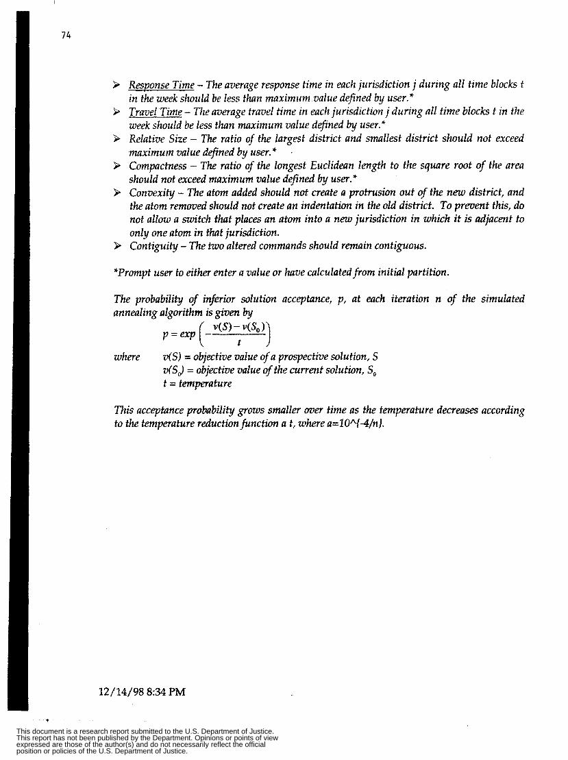
Response Time - The average response time in each jtirisdiction j during all time blocks t in the week should be less than maximum value defined by user.' Travel Time - The merage travel time in each jurisdiction j during all time blocks t in the week should be less than maximum value defined by user.* Relative Size - The ratio of the largest district and smallest district should not exceed maximum value defined by user. * Compactness - The ratio of the longest Euclidean length to the square root of the area should not exceed maximum value defined by user.* Convexity - The atom added should not create a protrusion out of the new district, and the atom remmed should not create an indentation in the old district. To prevent this, do not allow a switch that places an atom into a new jurisdiction in which it is adjacent to only one atom in that jurisdiction. Contiguity - The two altered commands should remain contiguous.
.
*Prompt user to either enter a value or have calculatedfrom initial partition.
The probability of inferior solution acceptance, p, at each iteration n of the simulated annealing algorithm is given by
where v(S) = objective value of a prospective solution, S v 6 J = objective value of the current solution, S, t = temperature
This accepfance probability gows smaller over time as the temperature decreases according to the temperature reductionfunction a t, where a=10A(-4/n).
12/14/98 8% PM
t
This document is a research report submitted to the U.S. Department of Justice.This report has not been published by the Department. Opinions or points of viewexpressed are those of the author(s) and do not necessarily reflect the officialposition or policies of the U.S. Department of Justice.
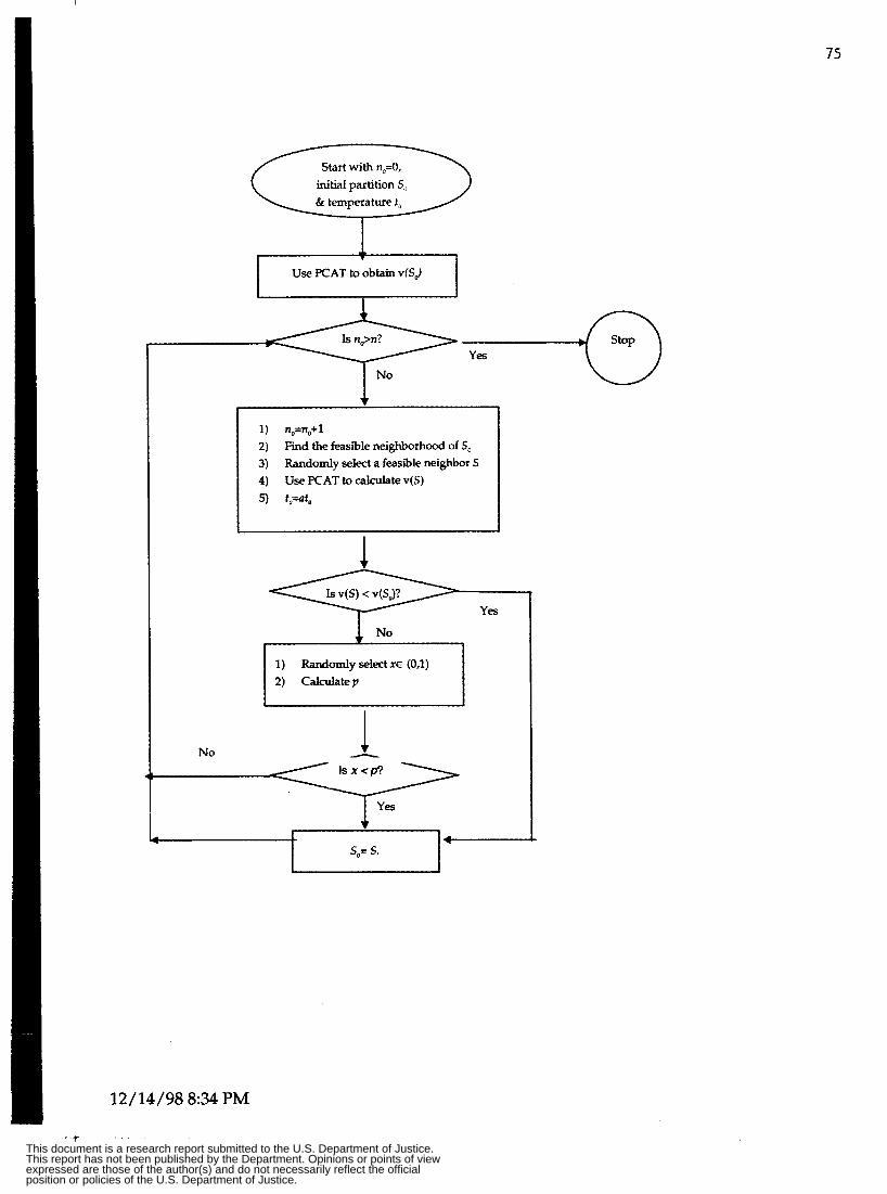
75
Start with n,=O, initial partition S,, & temperature tJ
. Use PCAT to obtain v(SJ
1) no=no+l 2) 3) 4)
Find the feasible neighborhood of So Randomly select a feasible neighbor S Use KAT to calculate v(S)
5) to=af,
1 Is v(S) < v(So)? Y YeS
1) Randomly select XE (0,l) 2) Calculatep I
I I
No -h- 1
Y so= s. l-
12/14/98 8:34 PM
This document is a research report submitted to the U.S. Department of Justice.This report has not been published by the Department. Opinions or points of viewexpressed are those of the author(s) and do not necessarily reflect the officialposition or policies of the U.S. Department of Justice.

I
76
- -* This document is a research report submitted to the U.S. Department of Justice.This report has not been published by the Department. Opinions or points of viewexpressed are those of the author(s) and do not necessarily reflect the officialposition or policies of the U.S. Department of Justice.
Appendix 2:
Flow Charts and GUIs
This document is a research report submitted to the U.S. Department of Justice.This report has not been published by the Department. Opinions or points of viewexpressed are those of the author(s) and do not necessarily reflect the officialposition or policies of the U.S. Department of Justice.
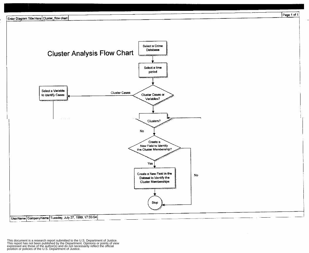
iter Diagram Tffle Here 1 Ciuster-flow chart I I -
__
Cluster Analysis Flow Chart
Select a Variable
i\ Create a /New Field to ldentifv \
Create a New Field in Dataset to Identify the Cluster Membership
No
This document is a research report submitted to the U.S. Department of Justice.This report has not been published by the Department. Opinions or points of viewexpressed are those of the author(s) and do not necessarily reflect the officialposition or policies of the U.S. Department of Justice.
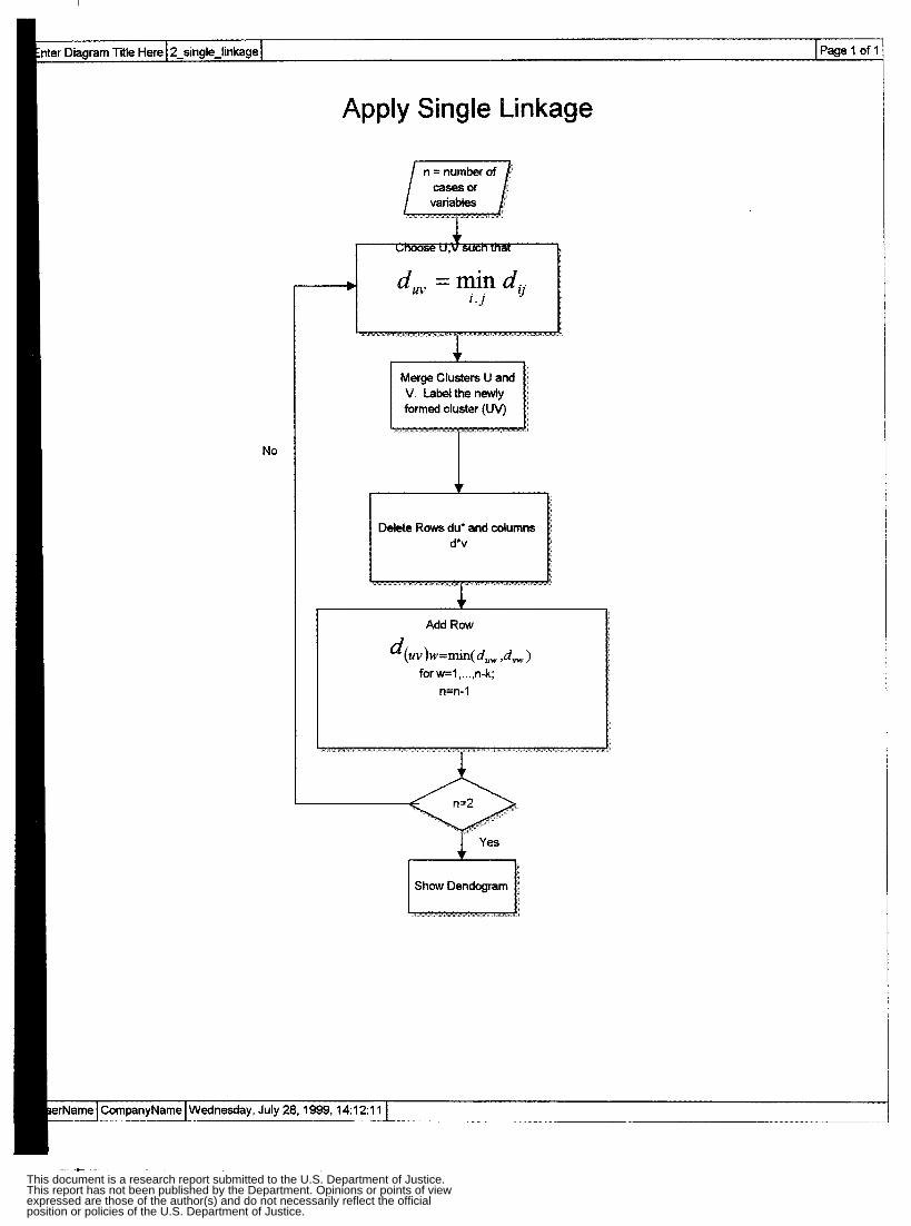
Apply Single Linkage
n = number of
I t
Merge Clusters U and V Labelthenewly
I
No
rName I CompanyName Wednesday, July 28,1999,14:12:11
I . I Delete Rows du' and columns
d*v
Add Row
for w=l ,..., n-k;
1 Yes
This document is a research report submitted to the U.S. Department of Justice.This report has not been published by the Department. Opinions or points of viewexpressed are those of the author(s) and do not necessarily reflect the officialposition or policies of the U.S. Department of Justice.
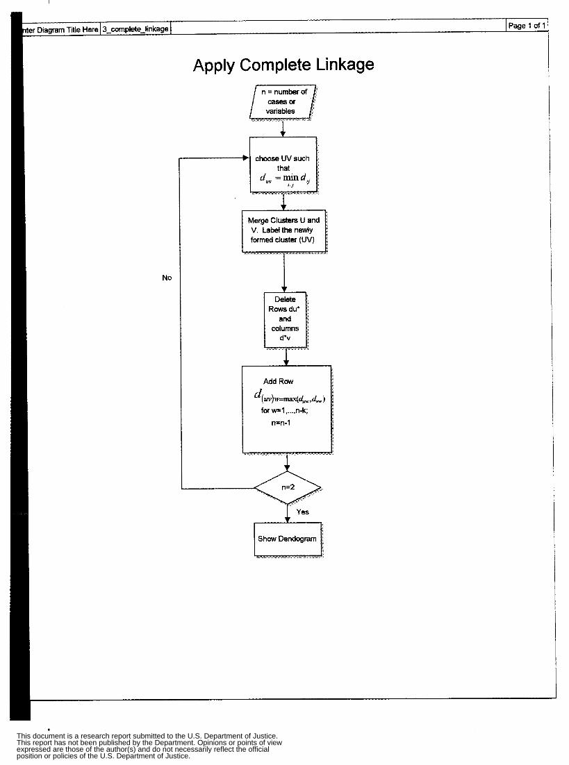
Apply Complete Linkage
Merge Clusters U and
formed cluster (UV)
I
NO
*
Add Row
This document is a research report submitted to the U.S. Department of Justice.This report has not been published by the Department. Opinions or points of viewexpressed are those of the author(s) and do not necessarily reflect the officialposition or policies of the U.S. Department of Justice.
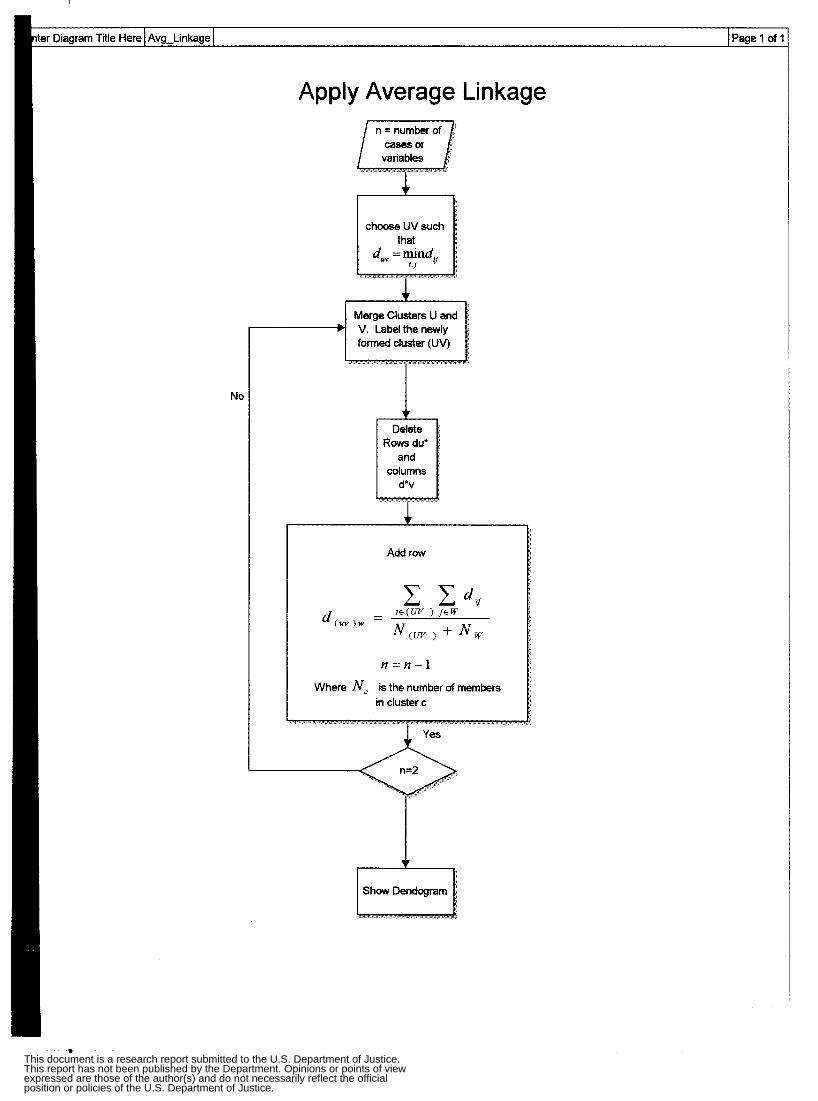
No
nter Diagram Title Here Avg-Linkage lpagel O ~ I
Apply Average Linkage
I MergeClustersUand I V. Label the newly formed cluster (UV)
(U" ) w
Add row
n = f l - l
Where NL is the number of members in cluster c
This document is a research report submitted to the U.S. Department of Justice.This report has not been published by the Department. Opinions or points of viewexpressed are those of the author(s) and do not necessarily reflect the officialposition or policies of the U.S. Department of Justice.
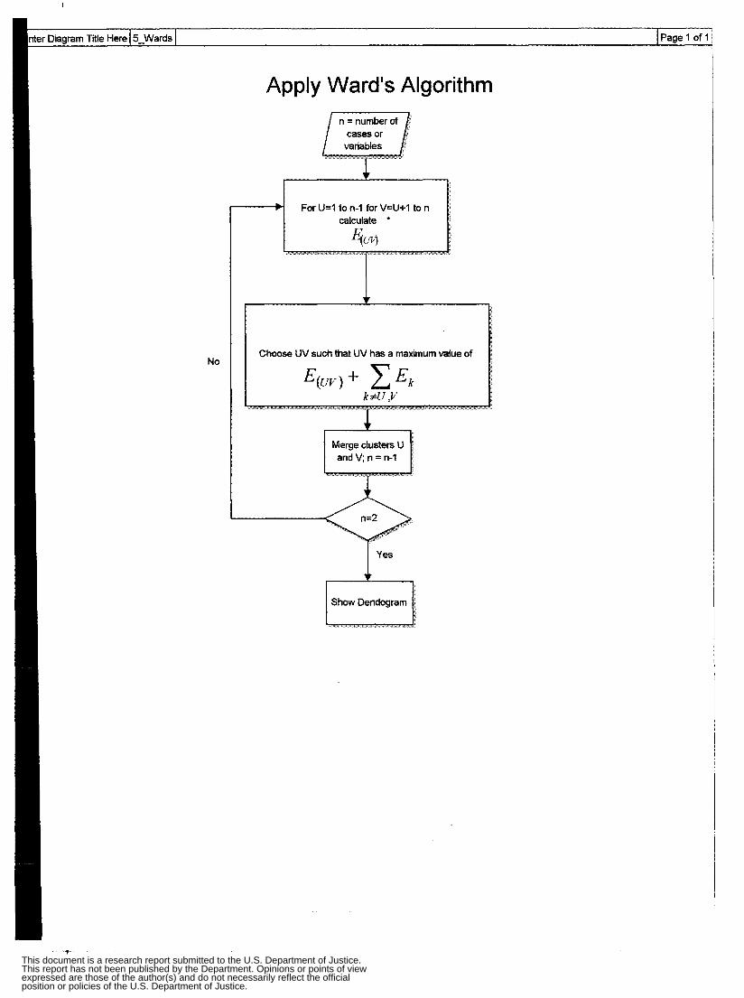
No
Apply Ward's Algorithm
For U=l to n-I for V=U+1 to n
Choose UV such that UV has a maximum value of
l-7 Merge clusters U
I yes
t This document is a research report submitted to the U.S. Department of Justice.This report has not been published by the Department. Opinions or points of viewexpressed are those of the author(s) and do not necessarily reflect the officialposition or policies of the U.S. Department of Justice.
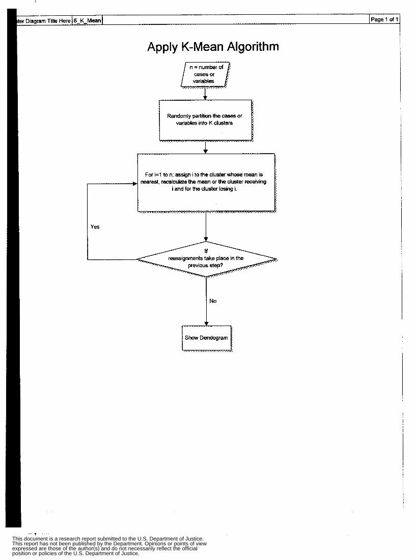
Apply K-Mean Algorithm
Randomly partition the cases or variables into K clusters
For 1=1 to n: assgn I to the cluster whose mean is nearest, recalculate the mean or the cluster rece~ving
i and for the cluster losing i.
Yes
reassignments take place in the
I No ~ Show Dendogram
t
This document is a research report submitted to the U.S. Department of Justice.This report has not been published by the Department. Opinions or points of viewexpressed are those of the author(s) and do not necessarily reflect the officialposition or policies of the U.S. Department of Justice.
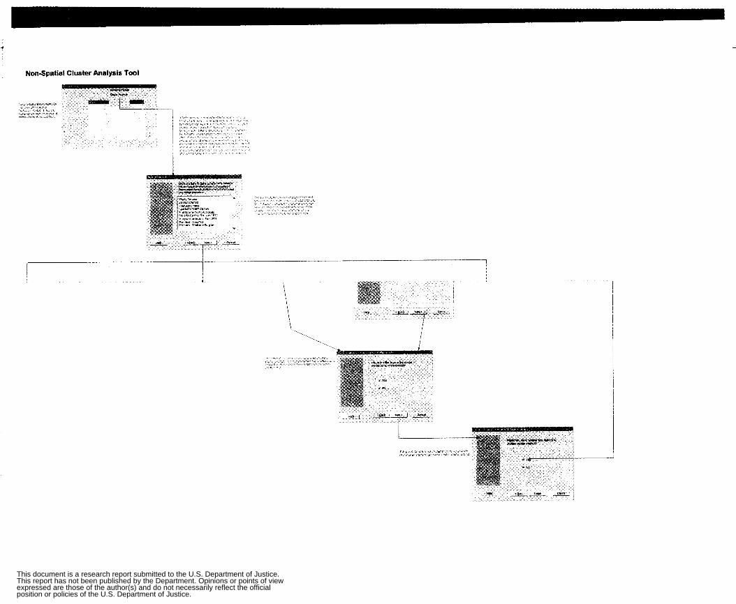
NonSpatial Cluster Analysis Tool
This document is a research report submitted to the U.S. Department of Justice.This report has not been published by the Department. Opinions or points of viewexpressed are those of the author(s) and do not necessarily reflect the officialposition or policies of the U.S. Department of Justice.
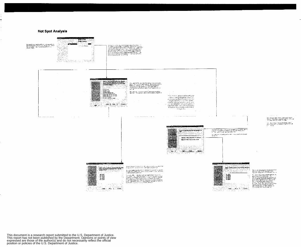
Hot Spot Analysis
. , . .. , , , . . . . ." ,,". .. , , . I , . . , . . , , . . r . .. .I , , . . . . $ .,. . . . . ,. - . .. .. ; , .,
, , . , . , , I :, I'
i
This document is a research report submitted to the U.S. Department of Justice.This report has not been published by the Department. Opinions or points of viewexpressed are those of the author(s) and do not necessarily reflect the officialposition or policies of the U.S. Department of Justice.

Page 1 of 1 nter Diagram Title Here I spatial-choro-flow test
serName
hloropleth Flow Chart
--____-- -_ CompanyName Wednesday, July 28,1999, I I :00:46 -~
Boundary Files: Census Block
Social Index, ; Arrests
Retrieve Boundary File Retrieve Census or Other
Snrinacnnornir natx
Calls-For-Service; Crime; Arrests
Query RMS by Location; Date; Time,
Type andfor M 0. I P
This document is a research report submitted to the U.S. Department of Justice.This report has not been published by the Department. Opinions or points of viewexpressed are those of the author(s) and do not necessarily reflect the officialposition or policies of the U.S. Department of Justice.
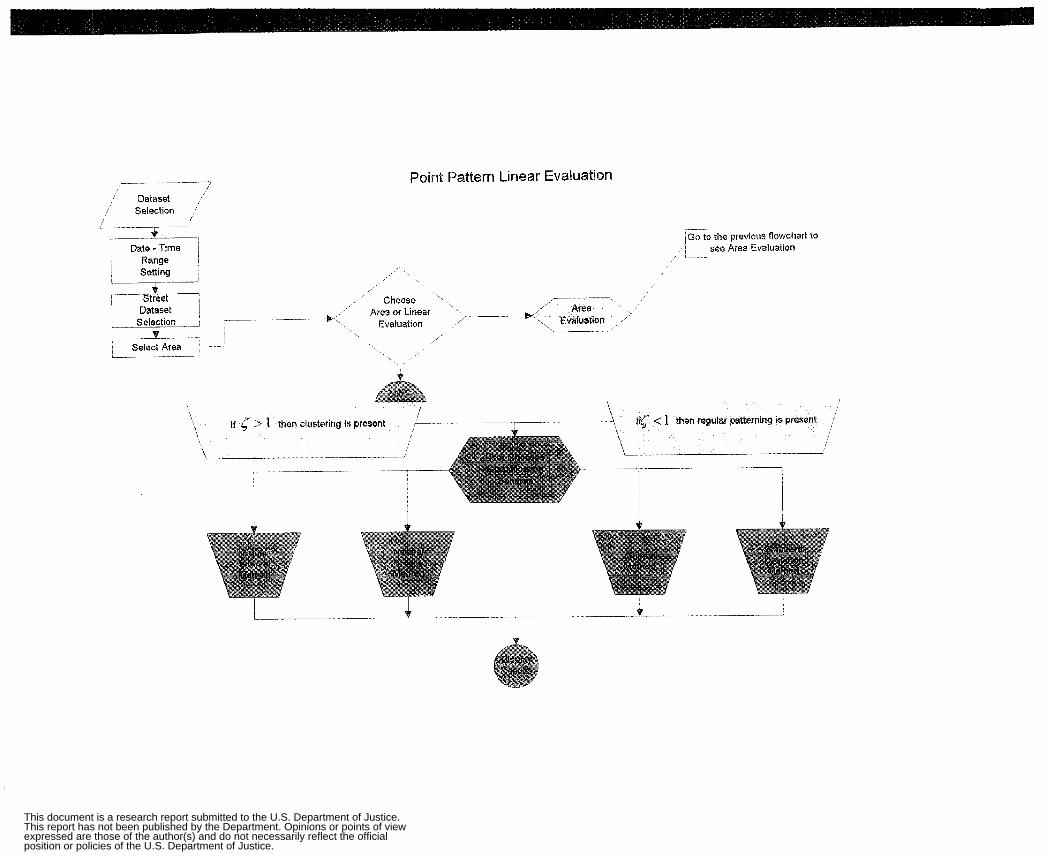
-3 -_ ,' Dataset '
I Selection /
Point Pattern Linear Evalu
'I G a t e - Time 1
Range ~
1 Setting
; Dataset i 1 Selection , ____ --
' Choose \
Area or Linear Evaluation
-___~ w: I
7- - J
If < 's 1 then clustering is present t
1
Go to the previous flowchart to '7 see Araa Evaluation , - -
\ i
I
*
This document is a research report submitted to the U.S. Department of Justice.This report has not been published by the Department. Opinions or points of viewexpressed are those of the author(s) and do not necessarily reflect the officialposition or policies of the U.S. Department of Justice.
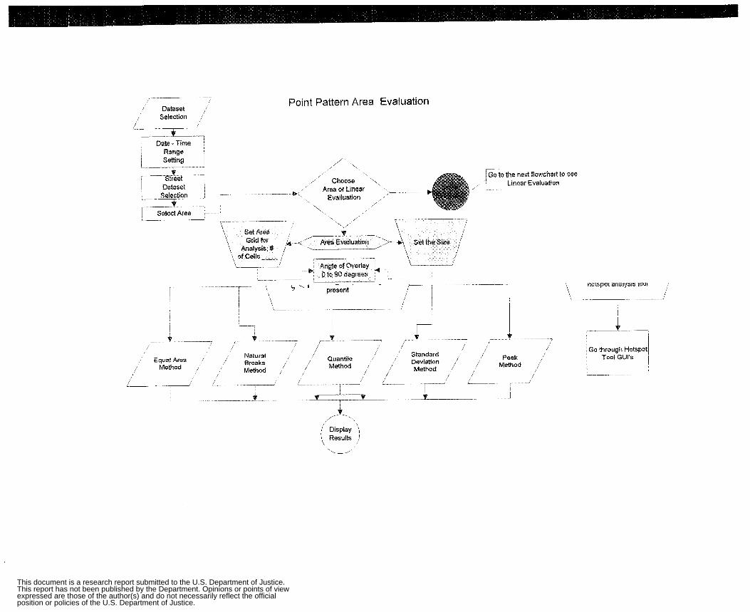
/ Dataset , Selection
Selection _ ~ _ -T __ I Select Area
Point Pattern Area Evaluation
,'
Area or Linear Evailuation
/Go to the next flowchart to see I Choose ,, i Linear Evaluation
.\,
i - _ -+, \
_____- e
f 1 -
~
I r- 1 f -- - + __ >---
i / ( / /- Peak , / Standard
/' Quanble Deviation Method
-e ~ _ - _ ~ _ _ --
/ Method Natural
Breaks / Method / Method , Equal Area
Method / / I
i- -- A-
i c-
,, norspar aiiaiysis toot \ , i
I
I
-1 \Go through Hotspot/
ToolGUl's \
,/ +- . Results )
This document is a research report submitted to the U.S. Department of Justice.This report has not been published by the Department. Opinions or points of viewexpressed are those of the author(s) and do not necessarily reflect the officialposition or policies of the U.S. Department of Justice.

inter Diagram Title Here
egression Regression
Determine where data is located .
R
I
Put up nonlinear screen.
UserName 1 CompanyName 1 Wednesday, July 28,1999,12:39:32 I -I - .-
This document is a research report submitted to the U.S. Department of Justice.This report has not been published by the Department. Opinions or points of viewexpressed are those of the author(s) and do not necessarily reflect the officialposition or policies of the U.S. Department of Justice.
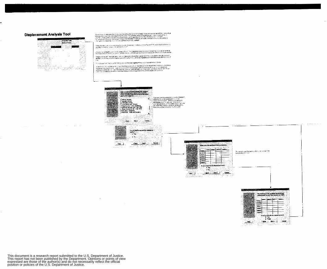
t
Displacement Analysis Tool
I I
This document is a research report submitted to the U.S. Department of Justice.This report has not been published by the Department. Opinions or points of viewexpressed are those of the author(s) and do not necessarily reflect the officialposition or policies of the U.S. Department of Justice.
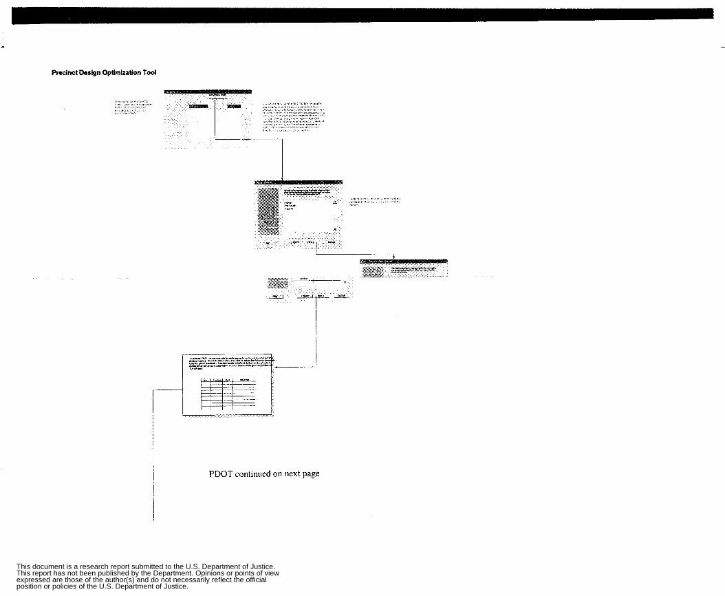
Precinct Design Optimization Tool
PDOT continued on next page
This document is a research report submitted to the U.S. Department of Justice.This report has not been published by the Department. Opinions or points of viewexpressed are those of the author(s) and do not necessarily reflect the officialposition or policies of the U.S. Department of Justice.
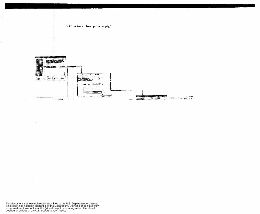
PDOT continued from previous page
This document is a research report submitted to the U.S. Department of Justice.This report has not been published by the Department. Opinions or points of viewexpressed are those of the author(s) and do not necessarily reflect the officialposition or policies of the U.S. Department of Justice.
Related Documents


