THÈSE EN COTUTELLE PRÉSENTÉE POUR OBTENIR LE GRADE DE DOCTEUR DE L’UNIVERSITÉ DE BORDEAUX ÉCOLE DOCTORALE SCIENCES PHYSIQUES ET DE L’INGÉNIEUR Spécialité : Astrophysique, plasma, nucléaire ET DE L’INSTITUT NATIONAL DE LA RECHERCHE SCIENTIFIQUE PROGRAMME DE SCIENCES DE L’ÉNERGIE ET DES MATÉRIAUX Par Pilar PUYUELO VALDÉS Laser-driven ion acceleration with high-density gas-jet targets and application to elemental analysis Faisceaux d’ions accélérés par interaction d’un laser intense avec un jet de gaz dense et application à l’analyse élémentaire Sous la direction de : Fazia HANNACHI et Patrizio ANTICI Soutenue le 05 octobre 2020 à l’Université de Bordeaux Membres du jury : Rapporteurs : M. Luca VOLPE Professeur CLPU Villamayor, Salamanca M. Alessandro FLACCO Maître de conférences LOA/ENSTA Palaiseau, Ile de France Examinateurs : M. Jean-Claude KIEFFER Professeur INRS Varennes, Montreal Mme. Sophie KAZAMIAS Professeure LASERIX Orsay, Ile de France Directeurs : Mme. Fazia HANNACHI Directrice de recherche CENBG Gradignan, Bordeaux M. Patrizio ANTICI Professeur INRS Varennes, Montreal Invité : M. Fabien DORCHIES Directeur de recherche CELIA Talence, Bordeaux

Welcome message from author
This document is posted to help you gain knowledge. Please leave a comment to let me know what you think about it! Share it to your friends and learn new things together.
Transcript

THÈSE EN COTUTELLE PRÉSENTÉE
POUR OBTENIR LE GRADE DE
DOCTEUR DE L’UNIVERSITÉ DE BORDEAUX
ÉCOLE DOCTORALE SCIENCES PHYSIQUES ET DE L’INGÉNIEUR Spécialité : Astrophysique, plasma, nucléaire
ET DE L’INSTITUT NATIONAL DE LA RECHERCHE
SCIENTIFIQUE
PROGRAMME DE SCIENCES DE L’ÉNERGIE ET DES MATÉRIAUX
Par Pilar PUYUELO VALDÉS
Laser-driven ion acceleration with high-density gas-jet targets and application to elemental analysis
Faisceaux d’ions accélérés par interaction d’un laser
intense avec un jet de gaz dense et application à l’analyse élémentaire
Sous la direction de : Fazia HANNACHI et Patrizio ANTICI
Soutenue le 05 octobre 2020 à l’Université de Bordeaux Membres du jury :
Rapporteurs : M. Luca VOLPE Professeur CLPU Villamayor, Salamanca
M. Alessandro FLACCO Maître de conférences LOA/ENSTA Palaiseau, Ile de France Examinateurs : M. Jean-Claude KIEFFER Professeur INRS Varennes, Montreal Mme. Sophie KAZAMIAS Professeure LASERIX Orsay, Ile de France Directeurs : Mme. Fazia HANNACHI Directrice de recherche CENBG Gradignan, Bordeaux M. Patrizio ANTICI Professeur INRS Varennes, Montreal Invité : M. Fabien DORCHIES Directeur de recherche CELIA Talence, Bordeaux


III
No hay mal que por bien no venga.
Confinement 2020
A mis padres, por apoyarme siempre e incondicionalmente.


V
ABSTRACT
In this joint thesis, performed between the French Institute CENBG (Bordeaux) and the
Canadian Institute INRS (Varennes), laser-driven ion acceleration and an application of the
beams are studied. The first part, carried out at CENBG and on the PICO2000 laser facility of
the LULI laboratory, studies both experimentally and using numerical particle-in-cell (PIC)
simulations, the interaction of a high-power infrared laser with a high-density gas target. The
second part, performed at ALLS laser facility of the EMT-INRS institute, investigates the
utilization of laser-generated beams for elementary analysis of various materials and
artifacts. In this work, firstly the characteristics of the two lasers, the experimental
configurations, and the different employed particle diagnostics (Thomson parabolas,
radiochromic films, etc.) are introduced.
In the first part, a detailed study of the supersonic high-density gas jets which have been
used as targets at LULI is presented, from their conceptual design using fluid dynamics
simulations, up to the characterization of their density profiles using Mach-Zehnder
interferometry. Other optical methods such as strioscopy have been implemented to control
the dynamics of the gas jet and thus define the optimal instant to perform the laser shot. The
spectra obtained in different interaction conditions are presented, showing maximum
energies of up to 6 MeV for protons and 16 MeV for helium ions in the laser direction.
Numerical simulations carried out with the PIC code PICLS are presented and used to
discuss the different structures seen in the spectra and the underlying acceleration
mechanisms.
The second part presents an experiment using laser-based sources generated by the ALLS
laser to perform a material analysis by the Particle-induced X-ray emission (PIXE) and X-ray
fluorescence (XRF) techniques. Proton and X-ray beams produced by the interaction of the
laser with aluminum, copper and gold targets were used to make these analyzes. The
relative importance of XRF or PIXE is studied depending on the nature of the
particle-production target. Several spectra obtained for different materials are presented and
discussed. The dual contribution of both processes is analyzed and indicates that a
combination improves the retrieval of constituents in materials and allows for volumetric
analysis up to tens of microns on cm2 large areas, up to a detection threshold of ppms.

VI
RESUME
Cette thèse en cotutelle entre la France et le Canada étudie l’accélération d’ions dans
l’interaction laser-plasma. La première partie, réalisée au CENBG et sur l’installation
PICO2000 du laboratoire LULI à l'École Polytechnique de Palaiseau, présente des études
expérimentales, complétées par des simulations numériques de type Particle-In-Cell, portant
sur l’accélération d’ions dans l'interaction d'un laser infrarouge de haute puissance avec une
cible gazeuse de haute densité. La seconde, réalisée avec le laser ALLS de l’institut EMT
INRS, concerne le développement d'une application des faisceaux génerés par laser pour
l’analyse élémentaire d’échantillons. Dans le manuscrit, les caractéristiques des deux lasers,
des différents diagnostics de particules et d’X utilisés (paraboles de Thomson, films
radiochromiques, CCD...) ainsi que les configurations expérimentales sont décrites.
Les jets de gaz denses supersoniques utilisés comme cibles d'interaction laser au LULI, sont
présentés en détail; depuis leur conception grâce à des simulations de dynamique des
fluides, jusqu’à la caractérisation de leurs profils de densité par interférométrie Mach
Zehnder. D'autres méthodes optiques comme la strioscopie ont été mises en œuvre pour
contrôler la dynamique du jet de gaz et définir l’instant optimal pour effectuer le tir laser. Les
spectres obtenus dans differentes conditions d’interaction sont présentés. Ils montrent, dans
la direction du laser, des énergies maximales allant jusqu’à 6 MeV pour les protons et 16
MeV pour les ions hélium. Des simulations numériques effectuées avec le code PICLS sont
utilisées pour discuter les différentes structures observées dans les spectres et les
mécanismes d’interaction sous jacents.
Des faisceaux de protons et d’X générés par le laser ALLS dans l’interaction avec des cibles
solides d’aluminium, de cuivre et d’or ont été utilisés pour effectuer des analyses de
matériaux par les méthodes Particle-induced X-ray emission (PIXE) et X-ray fluorescence
(XRF). L’importance relative des deux techniques, XRF et PIXE, est étudiée en fonction de la
nature de la cible d’interaction. Les deux diagnostics peuvent être implémentés
simultanément ou individuellement, en changeant simplement la cible d'interaction. La
double contribution des deux processus améliore l’identification des constituants des
matériaux et permet une analyse volumétrique jusqu'à des dizaines de microns et sur de
grandes surfaces (~cm2) jusqu'à un seuil de détection de quelques ppms.

VII
RESUMEN
En esta tesis doble, realizada entre el laboratorio francés CENBG y el Instituto canadiense
INRS, se ha estudiado la aceleración de iones impulsados por un láser infrarrojo de alta
potencia y una aplicación de los haces generados. En la primera parte, llevada a cabo en el
CENBG y en la instalación láser PICO2000 del laboratorio LULI, se ha estudiado
experimentalmente la interacción de este laser con un gas de alta densidad. En la segunda
parte, realizada con el láser ALLS del instituto EMT-INRS, se ha investigado la utilización de
haces generados por láser para el análisis elemental de diversos materiales y artefactos. En
primer lugar, se presentan las características de los dos láseres, las configuraciones
experimentales y los diferentes detectores empleados (parábolas de Thomson, RCF, etc.).
En la primera parte, se presenta un estudio detallado de los gas supersónicos de alta
densidad que se han utilizado como blancos en el LULI, desde su diseño utilizando
simulaciones de dinámica de fluidos, hasta la caracterización de sus perfiles de densidad
utilizando interferometría Mach-Zehnder. Se han implementado otros métodos ópticos,
como la estrioscopia, para controlar la dinámica del gas y, por lo tanto, definir el instante
óptimo para realizar el disparo con láser. Se pueden encontrar los espectros obtenidos en
diferentes condiciones de interacción. Muestran energías de hasta 6 MeV para protones y 16
MeV para iones de helio en la dirección del laser. Las simulaciones numéricas realizadas con
el código PICLS son presentadas y utilizadas para discutir las diferentes estructuras vistas en
los espectros y los mecanismos de aceleración subyacentes.
En la segunda parte se presenta un experimento utilizando los haces generados por el láser
ALLS para realizar el análisis de distintos materiales mediante las técnicas de emisión de
rayos X inducida por partículas (PIXE) y fluorescencia de rayos X (XRF). Los haces de
protones y rayos X producidos por la interacción del láser con blancos de aluminio, cobre y
oro se utilizaron para realizar estos análisis. La importancia relativa de XRF o PIXE ha sido
estudiada según la naturaleza del blanco. En esta parte se presenta y discute varios espectros
obtenidos para diferentes muestras. También se ha analizado la doble contribución de ambos
procesos. La combinación de ambos mejora la recuperación de elementos en los materiales y
permite el análisis volumétrico de hasta decenas de micras en grandes áreas, hasta un
umbral de detección del orden de ppms.


IX
LIST OF PUBLICATIONS
This thesis is based on the following publications, which are referred to by their Roman
numerals:
I. Optimization of critical-density gas jet targets for laser ion acceleration in the
collisionless shockwave acceleration regime.
J.L. Henares, T. Tarisien, P. Puyuelo, J.R. Marquès, T. Nguyen-Bui, F. Gobet, X.
Raymond, M. Versteegen and F. Hannachi.
J. Phys.: Conf. Ser., vol. 1079, 012004 (2018).
II. Laser-driven ion acceleration in high-density gas jets.
P. Puyuelo-Valdes, J.L. Henares, F. Hannachi, T. Ceccotti, J. Domange, M. Ehret, E.
d'Humieres, L. Lancia, J.R. Marquès, J. Santos and M. Tarisien.
Proc. SPIE 11037, Laser Acceleration of Electrons, Protons, and Ions V, 110370B, (2019).
III. The laser-driven ion acceleration beamline on the ALLS 200 TW for testing
nanowire targets.
S. Vallieres, P. Puyuelo-Valdes, M. Salvadori, C. Bienvenue, S. Payeur, E.
d’Humieres, and P. Antici.
Proc. SPIE 11037 Laser Acceleration of Electrons,Protons, and Ions V, 1103703, (2019).

X
IV. Development of critical-density gas jet targets for laser-driven ion acceleration.
J.L. Henares, P. Puyuelo-Valdes, F. Hannachi, T. Ceccotti, M. Ehret, F. Gobet, L.
Lancia, J.R. Marquès, J. J. Santos, M. Versteegen and M. Tarisien.
Rev. Sci. Instrum, vol. 90, 063302, (2019).
V. Low-energy proton calibration and energy-dependence linearization of EBT-XD
Radiochromic films.
S. Vallières, C. Bienvenue, P. Puyuelo-Valdes, M. Salvadori, E.d'Humières, and P.
Antici.
Rev. Sci. Instrum., vol. 90, 083301, (2019).
VI. Proton acceleration by collisionless shocks using a supersonic H2 gas-jet target and
high-power infrared laser pulses.
P. Puyuelo-Valdes, J.L. Henares, F. Hannachi, T. Ceccotti, J. Domange, M. Ehret,
E. d’Humieres, L. Lancia, J.-R. Marquès, X. Ribeyre, J.J. Santos, V. Tikhonchuk, and
M. Tarisien.
Phys. Plasma, vol. 26, 123109 (2019).
VII. Thomson Parabola and Time-Of-Flight Detectors Cross-Calibration Methodology on
the ALLS 100 TW Laser-Driven Ion Acceleration Beamline.
S. Vallières, M. Salvadori, P. Puyuelo-Valdes, S. Payeur, S. Fourmaux, F. Consoli, C.
Verona, E. d'Humières, M. Chicoine, S. Roorda, F. Schiettekatte, and P. Antici.
Rev of Sci Instrum., vol. 91, 103303 (2020).
VIII. Combined Laser based X-ray and Proton Induced Fluorescence: a versatile, fast,
multi- element analysis tool for investigation of artifacts.
P. Puyuelo-Valdes, S. Vallières, M. Salvadori, S. Payeur, S. Fourmaux, J.-C. Kieffer,
F. Hannachi, and P. Antici.
Submitted (2020).

11
ACKNOWLEDGE
I would like to acknowledge first the members of the jury for their careful reading and their
suggestions.
Je souhaite également remercier le CENBG de m'avoir accueilli chaleureusement et plus
particulièrement Nadine, parce que sans elle les choses ne se seraient pas si bien passées. Je
remercie également tout le groupe ENL pour m'avoir fourni le pilier nécessaire pour ne pas
me perdre en chemin. Un grand merci à Fazia pour son aide et ses précieux conseils qui
m’ont guidés tout au long de la thèse. Merci aux collaborateurs, par exemple Vladimir, qui a
été toujours disponible pour parler avec nous de théorie et il a eu la gentillesse de corriger
mon chapitre théorique de thèse. Je remercie également les personnes qui m'ont accompagné
dans les expériences, par exemple Jean Raphael et Livia, qui étaient mes premiers profs de
manips. J'ai passé un si bon moment ces semaines à Paris, et ce n'était pas seulement grâce à
la Tour Eiffel ! Je vous le garantie !
Un grand merci au groupe de l’INRS pour avoir rendu cette expérience universelle. Merci à
Patrizio pour m'avoir aidé à élargir ma vision de la thèse ainsi que pour nous avoir offert des
barres de chocolat dans le froid Canadien. De même à Simon, ta présence dans le groupe a
été essentielle. Sans ton aide, je n'aurais pas pu faire tout le développement de la simulation
et la boule rouge serait toujours un projet. Also thank you Martina, to bring calm and
precision to the group. Je voudrais remercier Stéphane, Leo, Sylvain, François Vidal et toutes
les personnes qui m’ont appris et aidé durant mon séjour à l’INRS. Dommage que le Canada
ne soit pas plus proche, et que l'INRS-EMT soit si loin de Montréal. Les deux métros et le bus
ne vont pas être faciles à oublier.

12
Je ne peux pas oublier tous ces gens qui, même s’ils n'appartenaient pas à mon groupe,
m'ont diverti pendant les repas et même pendant quelques dîners : Ricardo, Ana, Herve,
Jérémie, Yoandris, Elena, Uriel, Elissa, Angel et bien d'autres.
Gracias a mis profesores de toda la vida, de Zaragoza, en especial a Sebastián y a Pedro.
Gracias Sebas por hacerme que me gustase el láser y gracias Pedro por soportar mis quejas
durante toda la carrera. Seguidos de los profesores de Salamanca: Carlos, Iñigo, Julio, Ana,
Enrique … tenéis uno de los mejores másteres y no pude disfrutarlo más. También debo
agradecer a mis compañeros de máster y amigos que me acompañaron en ese año
maravilloso y que me siguen acompañando ahora también: Aurora, Alex, MA, JuanMi,
Roberto, Laura, Mario etc.
Con especial hincapié, dar las gracias a José, a su pack Esther y a su gordita Muriel, por
hacerme sentir como en casa tanto dentro como fuera del trabajo. Gracias José por tu
paciencia y por todas las veces que me preguntabas si necesitaba ayuda, estos años no
habrían sido iguales sin ti. Así como fuera, junto con Esther, habéis sido un apoyo
grandísimo para superar estos años en la lluviosa Francia. No podría haber deseado una
mejor familia.
No me puedo olvidar de personas que también han sido importantes en mi vida: biciclistas,
Aimar, Barbara, amigos de Logroño y Zaragoza que cada vez veo menos pero que fueron
muy importantes en su momento y a toda la gente que olvido pero que ha aportado su
granito de arena en mi vida. También a Inés, por esas lecciones de inglés y pronunciación
que me ayudaron para tener la confianza necesaria durante la presentación.
También agradecer a mi familia: abuela, tíos, primos; a mis seres más cercanos: mi madre y
mi padre sobre todo, los que me creyeron capaces de hacer todo lo que quisiese y más. A mis
hermanos, porque sé que los tengo allí para que lo que los necesite, aunque no tenga ni idea,
ni la tendrán, de que va esta tesis. Y a mis dos personas favoritas: mi A y mi R. Quienes se
hicieron relevo en estos años para soportarme y apoyarme. Porque sin esas cenas, sesiones
de Netflix y discusiones por Skype no podría haber sobrevivido.
Gracias a todos por estar ahí cuando lo necesito. Por estar en los buenos y malos momentos
de esta tesis. He aprendido mucho… no solo de física sino también de personas.

13
Merci à tous d’avoir été là quand j’en ai eu besoin, dans les bons et les mauvais moments de
cette thèse. J’ai beaucoup appris … pas seulement de la physique mais aussi des personnes.


15
RESUME DE THESE EN FRANÇAIS
Depuis de nombreuses années, la communauté laser travaille au développement
d'accélérateurs de particules compacts. Les accélérateurs conventionnels arrivent à des
limites d'espace, et leur coût d'exploitation devient difficile à payer, en particulier pour ceux
nécessaires à l'accélération des particules à haute énergie. En 1979, Tajima et Dawson [1979]
ont introduit le concept d'accélération par champ de sillage laser (en anglais, Laser wake field
acceleration (LWFA)). Ils ont prédit que l'accélération des électrons est possible avec une
impulsion électromagnétique intense via une onde plasma. Les techniques basées sur le laser
peuvent produire des champs accélérateurs, de l'ordre de centaines de GV/m. C'est trois
ordres de grandeur de plus que le champ électrique maximum que les cavités résonantes des
accélérateurs conventionnels peuvent supporter. Les électrons atteignent des énergies
d'environ 8 GeV dans le vide en 20 cm. Cela réduit considérablement la quantité de blindage
nécessaire.
L'accélération des particules à des énergies élevées est observée avec des impulsions laser
de forte puissance d'une intensité ≥ 1018 W/cm2. En 1985, la technique d'amplification
d'impulsions pulsées (chirped pulse amplification (CPA)) était la clé pour obtenir des durées
d'impulsions laser femto-seconde avec une puissance ultra-élevée allant du térawatt au
pétawatt [Strickland 1985]. Cette invention a conduit Donna Strickland et Gérard Mourou à
partager le prix Nobel de Physique en 2018. L'idée était d'étirer temporairement l'impulsion
laser avant les étapes d'amplification et de la compresser en une courte impulsion par la
suite. L'intensité de l'impulsion lors de l'amplification est réduite de plusieurs ordres de
grandeur, permettant son amplification sans endommager le matériau d'amplification et sans
produire d'effets non linéaires indésirables. La figure 1 montre l'évolution de l'intensité du

16
laser dans le temps depuis le début des années 60 d'après [Mourou and Tajima 2012]. Une
fois la technique CPA apparue, l'intensité des lasers a augmenté de manière quasi-linéaire
avec le temps. On observe que le régime relativiste, dans lequel la vitesse des électrons dans
le champ laser est proche de la vitesse de la lumière, peut être obtenu avec des impulsions
laser focalisées à une intensité minimale de 1018 W/cm2.
Figure 1. Évolution de l'intensité laser de 1960 à 2012. Modifié de [Mourou and Tajima 2012].
Avec de telles intensités, l’accélération des protons est possible. Certaines des
caractéristiques du faisceau de protons produit par laser sont : de courtes durées de paquets
(jusqu'à quelques picosecondes à la source), des flux de particules élevés (jusqu'à 1013
protons/MeV/sr par tir) et de grandes plages d'énergie (jusqu'à 100 MeV). Un large éventail
de domaines scientifiques, de la science fondamentale à la médecine, peut bénéficier de cette
nouvelle génération d'accélérateurs compacts.
Pour des intérêts médicaux, par exemple, l'interaction de protons avec des énergies de
quelques MeV avec certains matériaux peut produire des isotopes à courte durée de vie pour
les diagnostics par tomographie par émission de positons (positron emission tomography
(TEP)). Les principaux isotopes utilisés sont 11C (𝑇1/2= 20’), 13N (𝑇1/2= 10’), 15O (𝑇1/2= 2’), et 18F
(𝑇1/2= 110’). Pour des utilisations pratiques, des isotopes à courte durée de vie doivent être
produits à proximité des centres de thérapie médicale. Les accélérateurs d'ions par laser
Years

17
peuvent être déployés facilement. Dans le même domaine, le dépôt d'énergie des protons
dans la matière présente un intérêt pour la thérapie du cancer. La plupart de leur énergie est
délivrée à la fin de leur trajet (dans le pic de Bragg), ce qui est diffèrent du dépôt d'énergie
continue des électrons ou des rayons X dans la matière. Les courbes de dépôt de dose
correspondantes sont illustrées sur la figure 2. Le dépôt d'énergie localisé des ions permet de
détruire les tumeurs mais limite la dose délivrée aux cellules saines.
Figure 2 Exemple de dépôt d'énergie pour les protons (150 MeV) dans l'eau par rapport aux rayons X (20 et
4 MeV) et aux électrons (4 MeV).
Cette dernière propriété est également utile pour la fusion nucléaire induite par laser. Roth
et al. [2001] ont suggéré d'utiliser un faisceau de protons multi MeV produit avec un laser
pétawatt comme faisceau d'allumage pour créer un point chaud dans le carburant.
Les faisceaux d'ions sont également utiles pour la caractérisation non destructive des
matériaux, ce qui est important pour la recherche fondamentale et pour un large éventail
d'applications, notamment l'analyse d'échantillons biomédicaux, les études du patrimoine
culturel etc. Par exemple, la technique d'analyse par émission de rayons X induite par des
particules accélérées par laser (laser induced particle induced X ray emission, Laser-PIXE) a été
présentée par plusieurs groupes au cours des dernières années [Barberio 2017, Passoni 2019].
L'accélération des particules par laser est donc intéressante. Cependant, les faisceaux émis
doivent être bien caractérisés, stables, avec des distributions d'énergie bien définies et être

18
produits à un taux de répétition élevé. Cela a déclenché une série de nouvelles installations
laser produisant des impulsions courtes (ps-fs) de haute intensité (> 1018 W/cm2) avec des
taux de répétition plus élevés (comme APOLLON en France, les piliers ELI en Europe,
VEGA en Espagne, ALLS au Canada). Le taux de répétition de la génération précédente était
d'environ un à deux coups par heure.
Cette thèse présente l'étude des mécanismes d'accélération d’ions basés sur les lasers,
fournissant des énergies d’ions de l’ordre de quelques dizaines de MeV et facilement gérable
à HRR et l'une de leurs applications. La structure de cette thèse est la suivante : Après un
premier chapitre d’introduction.
Le chapitre 2 présente le contexte théorique qui permet de décrire l'interaction laser-plasma
et les processus d'accélération des protons. Nous nous concentrons sur ceux qui intéressent
ce travail de thèse.
Le chapitre 3 est dédié à la présentation des méthodes expérimentales développées ou
utilisées dans ce travail de thèse : la description du laser, le développement de la cible
d'interaction et les détecteurs. Les jets de gaz supersoniques à haute densité utilisés comme
cibles d'interaction sont une alternative intéressante pour l'accélération de différentes espèces
ioniques car ils peuvent être utilisés à HRR et sont exempts de débris. Cette partie du
chapitre est basée sur les papiers I et IV.
Notre objectif était de produire des profils de densité de gaz avec une densité maximale
d'environ 1021 cm−3 et une largeur a mi hauteur minimale (de l'ordre de 100 µm). Par
conséquent, des buses à gaz supersoniques ont été conçues. Il est important de noter que les
buses commerciales répondant à ces deux exigences ne sont pas faciles à trouver.
Trois types de buses supersoniques micrométriques ont été conçues à l'aide de simulations
de dynamique des fluides : les buses coniques, les buses à choc et les buses asymétriques.
Nous avons étudié en profondeur l'optimisation des paramètres des buses pour les deux
premiers types. Une comparaison de leurs profils de densité transversale et longitudinale a
également été effectuée. Les buses non axisymétriques sont plus difficiles à simuler car les
simulations CFD 3D prennent du temps.

19
Afin de valider les résultats, les profils de densité de gaz délivrés par les buses coniques ont
été mesurés avec un interféromètre Mach-Zehnder utilisant différents gaz. Des informations
sur la tomographie 3D avec des buses non axisymétriques ont également été rapportées.
Dans tous les cas, un bon accord a été trouvé entre les simulations et les mesures, ce qui a
validé la procédure.
Une caractérisation rigoureuse de la dynamique du flux gazeux est obligatoire pour
déclencher l'interaction laser à la densité maximale de la cible du gaz. L'évolution du flux
gazeux a été mesurée par strioscopie. Nous avons observé l'évolution de l'écoulement des
gaz d'hydrogène, d'azote et d'hélium pour différentes durées de temps d'ouverture des
électrovannes. Il faut plusieurs ms (110 ms pour N2 et ~ 60 ms pour H2 et He) pour remplir le
volume du réservoir de la buse et atteindre la densité maximale. Afin d'utiliser ces cibles de
gaz à haute répétition, la durée d'ouverture de la vanne (topen = 40 ms pour H2 et He et 80 ms
pour N2) sera réduite à l'avenir en réduisant le volume du réservoir de la buse.
Le chapitre 4 décrit les résultats expérimentaux de l'interaction du laser infrarouge
PICO2000 de haute puissance et des cibles à jet de gaz supersoniques conçues. Ce chapitre
fait référence aux papiers II et VI.
Deux campagnes expérimentales ont été réalisées. Dans la première campagne, nous avons
étudié des buses coniques de différentes tailles et des buses asymétriques pour sélectionner
les meilleurs paramètres pour l'accélération des ions. La plupart des interactions laser ont été
réalisées avec de l’hydrogène pur.
Nous avons observé des pics intéressants dans les spectres dans le cas de buses
asymétriques d'une énergie de 3,9 MeV à 0˚. Cependant, la caractérisation de ces buses est
plus difficile que pour les buses coniques et leur alignement n'était pas assez précis en raison
de contraintes mécaniques. C'est pourquoi, bien que ces cibles puissent être prometteuses, les
buses asymétriques n'ont pas été étudiées plus en détail.
Dans la 2ème campagne, de petites buses coniques ont été utilisées car elles ont donné des
flux de protons élevés avec une bonne répétabilité dans la première campagne. Leur
alignement et leur caractérisation étaient faciles et une petite quantité de gaz a été introduite
dans la chambre à vide. La livraison de trop de gaz dans la chambre expérimentale a produit

20
plusieurs claquages électriques dans les Thomson parabolas (TP). Au cours de la deuxième
campagne, des imaging plates MS-IP ont été utilisées comme détecteurs pour améliorer le
rapport signal/bruit de la détection. Nous avons gagné un ordre de grandeur au niveau du
fond. Cependant, les protons de basse énergies inférieures à 0,7 MeV n'étaient pas
détectables puisqu'ils sont arrêtés dans la couche de protection avant de l’IP MS. Dans la
première campagne, des dommages à la buse ont été observés après chaque tir. Pour la
deuxième, nous avons modifié les buses coniques pour avoir un profil de densité similaire
mais à une hauteur de tir de 400 µm par rapport à la sortie de la buse (au lieu de 200 µm).
Dans cette campagne, nous avons constaté que la focalisation du laser sur la pente
ascendante du profil de densité du jet de gaz fournit des protons plus énergétiques. Nous
avons également constaté que la réduction du niveau ASE au minimum réalisable était un
avantage pour l'accélération des protons dans la direction longitudinale. En résumé, une
accélération isotrope a été observée avec un flux de 1011 protons/MeV/sr à de faibles énergies
jusqu'à 1,5 MeV. Des structures à flux constant de particules (plateau) ont été observées dans
le sens transversal. Dans les meilleures conditions, une énergie maximale de 6 MeV a été
rapportée dans la direction longitudinale. Auparavant, en utilisant des cibles H2 à haute
densité, une énergie maximale de seulement 0,8 MeV était obtenue dans la direction
longitudinale [Chen 2017].
Des simulations hydrodynamiques 3D ont été utilisées pour comprendre l'évolution du
profil de densité du jet de gaz dû à l'interaction avec le laser ASE. Le profil de densité a été
significativement modifié et n'était plus gaussien. Un côté du profil de densité a été
radicalement transformé et un pic d'environ deux fois la densité d'origine s'est formé.
L'emplacement exact de ce pic n'a pas été bien défini car il dépend de la durée ASE qui n'a
pas été bien mesurée dans l'expérience.
Une fois que nous avons calculé la forme de la cible, des simulations PIC 2D ont été
effectuées pour interpréter les spectres de protons mesurés et être en mesure d'expliquer les
différents mécanismes d'accélération en jeu. L'auto-canalisation, l'auto-focalisation et la
multi-filamentation ont été trouvées dans les premières picosecondesde la simulation lorsque
le laser a interagi avec un plasma sous-dense. Ce fut l'origine des protons accélérés dans les
directions transversales. Les protons dans la direction longitudinale ont été accélérés en

21
raison du processus RPA-HB, induit par un changement radical du profil de densité. Le
processus a accéléré les protons à une énergie plus élevée et a créé des structures de plateau
dans les spectres. Des structures pointues à haute énergie ont été observées à différents
angles qui ont également été trouvés dans les simulations.
Certains tirs laser ont été réalisés avec une cible mixte de jet de gaz H2 et He. Dans ces cas,
des émissions de protons et d'hélium à tous les angles ont été observées. Environ
1012 protons ont été mesurés aux trois angles les plus avancés, tandis que le nombre de
particules émises à 90° est d'un ordre de grandeur inférieur. Au contraire, l'émission
transversale He2+ semblait plus importante que celle de 0°. De plus, presque aucun signal n'a
été observé à 30°, ce qui indique une émission plus collimatée. Ces observations sont
cohérentes avec les résultats rapportés dans les travaux précédents.
Chapitre 5
Le chapitre 5 présente une expérience utilisant des sources générées par le laser ALLS pour
effectuer une analyse de matériau par émission de rayons X induite par particules (PIXE) et
de fluorescence X (X ray fluorescence (XRF)). Ceci se réfère aux papiers VII et VIII.
Nous avons montré, pour la première fois à notre connaissance, expérimentalement et
numériquement (avec des simulations Geant4) que l'interaction d'un laser intense avec une
cible solide peut produire XRF et PIXE. Nous avons constaté que les deux techniques
d'analyse peuvent être mises en œuvre simultanément ou individuellement en quelques
secondes en changeant simplement le type de cible d'interaction (numéros atomiques
différents). Nous avons utilisé un échantillon d'acier inoxydable pour vérifier ce phénomène.
Nous avons trouvé une augmentation de l'intensité du spectre lorsque la cible Cu était
utilisée pour l'interaction laser par rapport au signal obtenu lorsque la cible Al (faible Z) était
utilisée. Nous avons pu confirmer les contributions relatives XRF et PIXE avec des
simulations Geant4, constatant que l'augmentation du signal était due à la contribution XRF.
Les rayons X de l’aluminium ne produisent aucune XRF détectable par notre diagnostic.
Nous avons également étudié la taille minimale de l'échantillon avec différents échantillons
de Ti pur. Cette technique permet d'analyser non seulement de grandes surfaces (le faisceau
de protons peut avoir une taille de spot de plusieurs cm) mais aussi des petites (par exemple

22
jusqu'à 9 mm2 dans le cas du Ti). Nous avons également constaté qu'il était possible de
détecter l'arsenic dans un échantillon de silicium dopé à l'arsenic avec un niveau de dopage
de 20 ppm, donnant le pourcentage de composition minimum détectable pour ce type
d'élément. De plus, nous avons étudié des échantillons non métalliques, dont le spectre a été
obtenu en une seule irradiation. Enfin, nous avons étudié le sondage volumétrique de
différentes piles d’éléments métalliques et de différentes pièces métalliques. Dans ce dernier
cas, nous avons pu identifier les pics liés à l'élément constitutif de chaque pièce.
Chapitre 6
Le chapitre 6 résume les résultats de ces travaux et les défis futurs associés aux cibles de jet
de gaz et aux techniques d'analyse dans les environnements laser.

23
CONTENTS
CHAPTER 1. INTRODUCTION .................................................................................................... 29
CHAPTER 2. LASER-MATTER INTERACTION ....................................................................... 35
2.1. Lasers: working principle................................................................................................. 35
2.2. Plasma description ............................................................................................................ 40
2.3. Single-electron interaction with an intense electromagnetic field in vacuum .......... 40
2.3.1. Motion of a free electron in an electromagnetic plane wave ............................ 42
2.3.2. Ponderomotive force .............................................................................................. 44
2.4. Laser interaction with low-density plasmas ................................................................. 45
2.4.1. Critical density ........................................................................................................ 45
2.4.2. Self-focusing ............................................................................................................. 46
2.4.3. Multi filamentation ................................................................................................. 47
2.5. Laser interaction with high-density plasmas ................................................................ 48
2.5.1. Absorption mechanisms ........................................................................................ 48
Collisional absorption .................................................................................. 49
Collisionless absorption ............................................................................. 50
Resonant absorption and inverse bremsstrahlung ......................................... 50
Vacuum plasma heating (Brunel mechanism) ................................................ 51
Relativistic 𝑱 × 𝑩 heating .................................................................................... 51
2.6. Hot electron generation .................................................................................................... 52

24
2.7. Generation of other particles and radiation .................................................................. 53
2.8. Ion acceleration mechanisms ........................................................................................... 54
2.8.1. Target Normal Sheath Acceleration (TNSA) ....................................................... 54
2.8.2. Radiation pressure acceleration (RPA) ................................................................ 57
Thick targets: Hole boring regime (RPA-HB) ......................................... 58
Thin targets: Light sail regime (RPA-LS) ................................................. 60
2.8.3. Collisionless shock acceleration (CSA) ................................................................ 60
2.9. Hydrodynamic simulations ............................................................................................. 62
2.10. Particle-In-Cell (PIC) simulation ................................................................................... 63
CHAPTER 3. EXPERIMENTAL METHODS ............................................................................... 67
3.1. Laser systems ..................................................................................................................... 67
3.1.1. PICO2000 laser system ........................................................................................... 68
3.1.2. ALLS 100 TW laser system .................................................................................... 69
3.2. Targetry: development of gas-jet targets ....................................................................... 71
3.2.1. Supersonic gas jets: definitions ............................................................................. 74
3.2.2. Study and optimization of nozzle geometric parameters ................................. 80
Conical nozzles .................................................................................................... 82
Shock nozzles ....................................................................................................... 85
Asymmetrical nozzles (AN) ............................................................................... 88
Remark concerning the gas reservoir design ................................................... 88
3.2.3. Transversal and longitudinal density profiles .................................................... 89
3.2.4. Remark concerning gas jets in air ......................................................................... 91
3.2.5. Conclusion ............................................................................................................... 92
3.2.6. Experimental characterization of the gas jet ....................................................... 94
Mach-Zehnder interferometer ........................................................................... 94
3D tomography .................................................................................................... 97

25
Dynamics of the gas jet ..................................................................................... 100
3.3. Particle and X-ray diagnostics ....................................................................................... 103
3.3.1. Passive detectors ................................................................................................... 103
Radiochromic films (RCF) ....................................................................... 103
Imaging plates (IP) .................................................................................... 105
3.3.2. Active detectors ..................................................................................................... 107
Scintillators ................................................................................................ 108
Micro-channel plate (MCP) ..................................................................... 108
CCD ............................................................................................................ 109
Diamonds ................................................................................................... 109
3.3.3. Spectrometers ........................................................................................................ 110
Time of flight (TOF) .................................................................................. 111
Thomson parabola (TP) ............................................................................ 112
CHAPTER 4. GAS TARGET EXPERIMENT RESULTS ........................................................... 119
4.1. Introduction ..................................................................................................................... 119
4.1. Experimental setup ......................................................................................................... 119
4.2. Laser-beam alignment and plasma diagnostics .......................................................... 121
4.3. Results on proton acceleration ...................................................................................... 125
4.3.1. 1st campaign ........................................................................................................... 125
4.3.2. 2nd campaign .......................................................................................................... 129
4.3.3. Hydrodynamic and PIC simulations ................................................................. 132
Laser interaction with the under-dense plasma ................................... 135
Laser interaction with the over-critical plasma .................................... 137
Longer times: laser beam collapse .......................................................... 140
Discussion .................................................................................................. 141
4.4. Results on helium acceleration ...................................................................................... 143

26
CHAPTER 5. Laser-based X-ray and Proton Induced Fluorescence (Laser-XPIF) analysis 147
5.1. Introduction ..................................................................................................................... 147
5.1.1. Particle-matter interaction ................................................................................... 148
Stopping power ......................................................................................... 148
5.1.2. Photon-matter interaction .................................................................................... 149
X-ray beam attenuation coefficient......................................................... 149
Interaction processes ................................................................................ 150
5.2. PIXE and XRF techniques............................................................................................... 151
5.2.1. Fluorescence yield and transition probability .................................................. 154
5.2.2. Fluorescence cross-sections ................................................................................. 155
5.2.1. Conventional PIXE and XRF sources and detectors ........................................ 157
5.2.2. Background ............................................................................................................ 158
5.2.3. Lower limits of detection ..................................................................................... 160
5.2.1. Penetration Depths ............................................................................................... 160
5.2.2. Flexibility ................................................................................................................ 161
5.3. Laser-based analysis technique ..................................................................................... 161
5.4. Experimental setup ......................................................................................................... 162
5.4.1. Spectrum reconstruction ...................................................................................... 163
5.4.2. Particle diagnostics ............................................................................................... 165
5.4.3. X-ray diagnostics ................................................................................................... 168
5.5. Results ............................................................................................................................... 170
5.5.1. PIXE and XRF contributions: XPIF technique ................................................... 170
5.5.2. Metallic samples .................................................................................................... 173
5.5.3. Minimum sample size .......................................................................................... 173
5.5.4. XPIF background .................................................................................................. 174
5.5.5. Minimum detectable composition ...................................................................... 175

27
5.5.6. Non-metallic samples ........................................................................................... 176
5.5.7. Volumetric probing............................................................................................... 177
5.5.8. Real-setting application: coins ............................................................................. 178
5.6. Conclusion ........................................................................................................................ 179
CHAPTER 6. CONCLUSION AND PERSPECTIVES .............................................................. 181
6.1. Ion acceleration with gas-jet targets ............................................................................. 181
6.1.1. Future approaches ................................................................................................ 184
How to avoid nozzle damage ................................................................. 184
How to enhance the longitudinal proton acceleration: Plasma shaping
............................................................................................................................................................. 186
6.2. XPIF analysis technique ................................................................................................. 188
6.2.1. Future approaches ................................................................................................ 189
Quantitative analysis ................................................................................ 189
Air XPIF ...................................................................................................... 189
PIXE at high laser repetition rate ............................................................ 190


29
CHAPTER 1.
INTRODUCTION
For many years, the laser community has been working on the development on compact
particle accelerators. Conventional accelerators are running into space limits, as they are up
to kilometer sizes, and their operating cost becomes difficult to afford, especially for those
required for high-energy-particle acceleration. In 1979, Tajima and Dawson [1979]
introduced the concept of Laser-wake-field acceleration (LWFA). They predicted that electron
acceleration is possible with an intense electromagnetic pulse via a plasma wave.
Laser-based techniques can produce high accelerating fields, of the order of hundreds of
GV/m. This is three orders of magnitude higher than the maximum electric field that
conventional accelerator resonant cavities can sustain. Electrons achieve energies of about
8 GeV in vacuum in 20 cm. Consequently, the radioactivity is only produced around the
acceleration area, which is smaller than in conventional accelerators.
Particle acceleration at high energies is observed with high-power laser pulses of an
intensity ≥1018W/cm2. In 1985, the chirped pulse amplification (CPA) technique was the key to
obtain down to femto-second laser pulse durations with ultra-high power from terawatt to
petawatt [Strickland 1985]. This invention led Donna Strickland and Gérard Mourou to share
the 2018 Physics Nobel Prize. The idea was to temporally stretch the laser pulse before the
amplification stages and compress it to a short pulse afterward. The intensity of the pulse
during the amplification is reduced by several orders of magnitude, allowing its

CHAPTER 1. INTRODUCTION
30
amplification without damaging the amplification material and without producing
unwanted nonlinear effects. Figure 1.1 shows the laser intensity evolution through time since
the early 60s from [Mourou and Tajima 2012]. Once the CPA technique had emerged, the
intensity of the lasers increased quasi-linearly with time. One observes that the relativistic
regime, in which the electron quiver velocity in the laser field is close to the speed of light,
can be achieved with laser pulses focused into an intensity of minimum 1018 W/cm2.
Figure 1.1. Laser intensity evolution from 1960 to 2012. Adapted from [Mourou and Tajima 2012].
With such high intensities, high-energy proton acceleration is possible. Some of the laser-
driven proton beam characteristics are: short bunch durations (up to few picoseconds at the
source), high particle fluxes (up to 1013 protons/MeV/sr per shot) and large energy ranges
(up to 100 MeV). A large range of science areas, from fundamental science to medicine, may
benefit from these new generation of compact accelerators.
For medical interests, for example, the interaction of MeV protons with some materials can
produce short-lived isotopes for positron emission tomography (PET) diagnostics. The principal
isotopes used are 11C (𝑇1/2 = 20’), 13N (𝑇1/2 = 10’), 15O (𝑇1/2 = 2’), and 18F (𝑇1/2 = 110’). For
practical uses, short-lifetime isotopes need to be produced close to medical therapy centers.
Laser-driven ion accelerators represent a good alternative. In the same field, the proton
energy deposition in matter is of interest for cancer therapy. Most of their energy is delivered
Years

CHAPTER 1. INTRODUCTION
31
at the end of their path (in the so-called Bragg peak), which is at variance with the
continuous energy deposition of electrons or X-rays. These are illustrated in Figure 1.2. This
peak energy deposition allows to destroy tumors and limits the dose delivered to the
surrounding healthy cells.
Figure 1.2 Example of energy deposition for protons (150 MeV) in water compared with X-rays (20 and 4 MeV)
and electrons (4 MeV). From wikicommons by Cepheiden.
This later property is useful also for laser-induced nuclear fusion. Roth et al. [2001]
suggested to use a multi-MeV proton beam produced with a petawatt laser as an ignitor
beam to create a hotspot in the fuel.
Ion beams are also useful for non-destructive material characterization, which is important
for basic research and for a wide range of applications, including analysis of biomedical
samples, cultural heritage studies, forensic analysis and so on. For example, Laser-based
particle induced X-ray emission (Laser-PIXE) analysis technique was presented by several
groups in the last years [Barberio 2017, Passoni 2019].
Laser-driven particle acceleration is therefore of interest. However, the emitted beams need
to be well-characterized, stable and with well-defined energy distributions and to be
produced at high repetition rate (HRR). This has triggered a series of new laser facilities
producing high-intensity (>1018 W/cm2) short pulses (ps-fs) with higher repetition rates. The
previous generation's repetition rate was about one to two shots per hour. Nowadays, VEGA

CHAPTER 1. INTRODUCTION
32
laser in Spain or ALLS laser in Canada are capable to deliver around 5 J in several tens of
femtosecond at 10 or 2.5 Hz respectively (200 TW). VEGA is expected to provide another
laser line with 30 J of energy at 1 Hz (1 PW). In addition, ELI pillar project is already building
100 TW laser at 10 Hz, 1 PW laser at 1 Hz and 3 PW at 1 pulse per minute repetition rate in
the Czech Republic, Hungary and Romania. In France, the APOLLON laser is as well under
construction. The main laser pulse will deliver 150 J in 15 fs (10 PW) at 1 shot per minute.
This thesis presents the study of laser-based ion acceleration mechanisms providing ion
energy of tens of MeV and easily manageable at HRR and one of their applications. The
structure of this thesis is as follows:
Chapter 2
Chapter 2 presents some theoretical background to describe laser-plasma interaction and
the proton acceleration processes. We concentrate meanly in the ones of interest for this
thesis work.
Chapter 3
Chapter 3 is dedicated to the presentation of the experimental methods developed or used
in this thesis work: the laser description, the interaction target development, and the
detectors. The supersonic high-density gas jets employed as interaction targets are an
interesting alternative for different ion species acceleration as they can be used at HRR and
are debris free. We detail their design and characterization since they are not usually
commercially available. This part of the chapter is based on Papers I and IV.
Chapter 4
Chapter 4 describes the experimental results of the interaction of the PICO2000 laser and
the designed supersonic gas-jet targets. The proton and He ion spectra obtained in different
interaction conditions (laser parameters and gas-jet density profiles) are presented.
Numerical simulations carried out with the hydrodynamic code FLASH and particle-in-cell
(PIC) code PICLS are performed. Their results are used to enlighten the origin of the

CHAPTER 1. INTRODUCTION
33
different structures seen in the spectra and the underlying acceleration mechanisms. This
chapter refers to Papers II and VI.
Chapter 5
Chapter 5 presents an experiment using laser-based sources generated by the ALLS laser to
perform a material analysis by the Particle-induced X-ray emission (PIXE) and X-ray
fluorescence (XRF) techniques. Proton and X-ray beams produced by the interaction of the
laser with aluminum, copper and gold targets were used to make these analyzes. The
relative importance of XRF or PIXE is studied depending on the nature of the
particle-production target. Several spectra obtained for different materials are presented and
discussed. The dual contribution of both processes is also analyzed and discussed. This
refers to Papers VII and VIII.
Chapter 6
Chapter 6 summarizes the findings of this work and the future challenges associated with
gas-jet targets and the analysis techniques in laser environments.


35
CHAPTER 2.
LASER-MATTER INTERACTION
2.1. Lasers: working principle
Lasers are versatile tools that can be used in many fields: industry (cutting, welding),
communication (optic fibers), medicine (cornea surgery, esthetic treatments), everyday life
(scanning technology, laser pointers) and research. The working principle of the laser is
based on three features: population inversion, stimulated emission in an amplifying medium
and optical resonator.
When an electron from a low-lying atomic state is transferred to an excited one, after
absorption of one or several photons, the electron in the excited state may spontaneously
decay to the ground state by photon emission. The photon energy is the difference between
the energies of the two states. This process is called spontaneous emission of fluorescence
light, each excited atom emits a photon independently. However, if the population of the
excited states is larger than the ground state ones, a stimulated emission is prominent. Hence,
a first photon emitted by an exited atom passes by the neighbor excited atom and provokes
emission of a second photon of the same frequency, in the same direction and in phase with
the first one. The two photons are coherent: they have the same frequency, polarization,
direction, and phase. This process proceeds in cascade. Namely, these two photons induce

CHAPTER 2. LASER-MATTER INTERACTION
36
emission of two more and so on. This is the so-called stimulated emission and it is at the
origin of the optical amplification. Figure 2.1 describes the different atom-photon interaction
mechanisms presented above: Figure 2.1a describes the absorption. Some atoms in a media
absorb photons and are transiting from the ground level 0 to a higher energy level 1. The
emission processes are presented in Figure 2.1b, the spontaneous emission, and Figure 2.1c,
the stimulated emission.
Figure 2.1 Interaction mechanisms between an atom and a photon (the photon has an energy ℎ𝜈 equal to the
difference between the two atomic level energies) between levels 0 and 1. a) shows the absorption, b) the
spontaneous emission and c) the stimulated emission. Figure taken from [Photonics 2016].
If the higher energy state has a greater population than the lower energy one, the population
inversion is achieved. With the population inversion, amplifying a photon signal by stimulated
emission is possible.
Figure 2.2. Scheme of multi-pass photon process in a laser cavity.
In a laser, the stimulated emission is produced spatially and temporally coherent in one
direction while spontaneous emission is produced in all directions. To generate a strong
signal, the amplifying medium is placed in an optical cavity equipped usually with two flat
or concave mirrors, that reflect the photons back and forth (see Figure 2.2, photons are
presented with red curvy arrows). The front mirror is made 99% reflective, hence some of the
100% reflective mirror
99% reflective mirror
Photons
Amplifying medium
Laser light
a) b) c)

2.1 Lasers: working principle
37
laser light is transmitted by the mirror. The multi-pass process, illustrated in Figure 2.2, has a
high gain.
Lasers can deliver continuous or pulsed light. Pulsed lasers concentrate their energy, 𝐸𝐿, in
pulses of duration 𝜏𝐿 at a repetition rate 𝑅𝐿 to achieve the highest optical powers., 𝑃𝐿 = 𝐸𝐿/𝜏𝐿.
This is achieved by the process of mode section in lasing cavity. These parameters are
represented in Figure 2.3, where the average intensity (𝐼𝑎𝑣𝑔) is plotted as well.
Figure 2.3 Representation of the laser pulse intensity. The repetition rate 𝑅𝐿 and the pulse duration 𝜏𝐿 are
represented in the image [the picture is taken from www.silloptics.de].
The temporal and spatial distributions of the laser pulse can be described by the electric
field of a monochromatic (and uniformly polarized) optical beam propagating at small
angles (i.e. paraxially) along the 𝑥-direction of an 𝑥𝑦𝑧 (𝒓) Cartesian system of coordinates
[LasersAndOpt 2012] (in the following, bold symbols represent vectors).
𝑬(𝒓, 𝑡) = 𝐸0 𝒆𝑦 𝒖(𝒓) 𝑒xp (𝑖𝑘𝐿𝑥 - 𝑖𝜔𝐿𝑡) where 𝜔𝐿 = 2𝜋𝑐/𝜆𝐿 is the laser frequency, 𝑘𝐿 = 2𝜋/𝜆𝐿 is
the wavenumber, 𝒖(𝒓) is the complex field envelope, 𝒆𝒚 is the polarization vector and 𝐸0 is
the maximum amplitude of the wave.
In the case of a Gaussian beam, 𝒖(𝒓) is expressed as:
𝒖(𝒓) = 𝑤0/𝑤(𝑥) exp(−(𝑧2 + 𝑦2)/𝑤2(𝑥)) exp (𝑖𝑘𝐿(𝑧
2 + 𝑦2)/(2𝑅(𝑥))) exp(𝑖𝜑(𝑥)) (2.1)
where 𝑤(𝑥) = 𝑤0 √1 + (𝑥/𝑧𝑅)2 is the transverse size of the beam and 𝑤(𝑥 = 0) = 𝑤0 (the
minimum spot size) is the beam waist; 𝑅(𝑥) = 𝑥 (1 + (𝑧𝑅/𝑥)2) is the radius of curvature of the
Pulse duration τL
Time between pulses = 1/repetition rate RL

CHAPTER 2. LASER-MATTER INTERACTION
38
beam wave front, 𝑧𝑅 = 𝜋𝑤02/𝜆𝐿 is the Rayleigh length and 𝜑(𝑥) = tan−1(𝑥/𝑧𝑅) is the beam
Gouy phase.
It is important to notice that the scalar field 𝒖(𝒓) depends on:
an amplitude factor with a transverse Gaussian distribution
𝑤0/w(𝑥) exp( - (𝑧2+𝑦2)/𝑤2(𝑥)) (2.2)
a transverse phase factor
exp (𝑖𝑘𝐿(𝑧2 + 𝑦2)/(2𝑅(𝑥)))
(2.3)
and a longitudinal phase factor
exp(𝑖𝜑(𝑥)) (2.4)
The transverse size, 𝑤, which is called the beam width, changes along the propagation in the
𝑥-axis (See Figure 2.4). At 𝑥 = 𝑧𝑅, the beam width has increased with respect to the beam waist
by a factor of √2,𝑤 = √2𝑤0. Because the beam tends to diffract, a new parameter is
introduced: the divergence of the laser beam, tan 𝜃𝐿 = 𝜆𝐿/(𝜋𝑤0), which is the ratio of the
beam width to the distance from the focal plane 𝑤(𝑥)/𝑥 at large distance, 𝑥 ≫ 𝑧𝑅. For real
laser beams, an 𝑀2 factor is defined as 𝑀2 = 𝜃𝐿𝜋𝑤0/𝜆𝐿, which characterizes the quality of the
beam. If 𝑀2 = 1 the beam is perfectly Gaussian.
Figure 2.4 Scheme of a laser beam propagation where 𝑤(𝑥) is the beam spot radius and 𝑤0 is the beam waist, 𝜃𝐿 is
the divergence and 𝑧𝑅 is the Rayleigh length.
𝑥
w 𝑥
𝜃𝐿𝑤02𝑤0
𝑧𝑅

2.1 Lasers: working principle
39
Since we usually measure the intensity of a laser beam, it is useful to define the peak
intensity of a Gaussian beam in the focal plane using the optical power and the beam waist:
𝐼𝐿 ≈0.5 𝑃𝐿/(𝜋𝑤02) . There is usually 40 or 50% of the laser energy in the central lobe due to
diffraction effects.
After the invention of the CPA technique [Strickland 1985], ultra-high-power laser pulses
could be produced without damaging the amplification material and the different optics
involved in the amplification process. Since then, high-power laser facilities have been built
all over the world. The characteristics of the lasers used in this thesis work are listed in Table
2.1.
PICO2000 ALLS
Laboratory LULI EMT-INRS
Country France Canada
Type Nd:Glass Ti:Saphire
𝝀𝑳 [𝐧𝐦] 1053 800
𝝉𝑳 [𝒔] 1 × 10⁻¹² 20 × 10−15
𝑻𝒎𝒂𝒙 1 shot/h 2.5 Hz
𝑬 [𝐉] 60 2
𝑰 [𝐖/𝐜𝐦𝟐] 5 × 10¹⁹ 1.3 × 10²⁰
Parabola f/4 f/3
Focal spot, FWHM [𝛍𝐦] 12 5
Contrast, 250 ps 10−6 10−9
Table 2.1 Characteristics of the PICO2000 and ALLS laser systems. FWHM means full width at half maximum.
The spontaneous emission that takes place in the laser process, limits the laser pulse
temporal intensity contrast. After the pulse compression, the amplified spontaneous emission
(ASE) results in a quasi-continuous pedestal which is partly located before the main pulse.
This is the incoherent contribution. Laser operators measure the relation between the pulse
intensity and the ASE by the so-called contrast. For example, ALLS laser has a ps contrast of
10−9 and a ns contrast of 10−11. The PICO2000 laser has a ps contrast of 10−6 and a ns contrast
of 10−8. At high intensity, in relativistic laser-matter interactions, the ASE plays an important
role as it modifies the target properties before the main pulse arrival.

CHAPTER 2. LASER-MATTER INTERACTION
40
2.2. Plasma description
In laser-based charged-particle acceleration, the interaction of the intense laser beam with
a target (e.g. a micrometric foil) generates a plasma.
Plasma is the fourth fundamental state of matter. It is a gas of ions and electrons coupled
with self-consistent electric and magnetic fields where free electrons screen the Coulomb
potential of the ions by their own Coulomb potential. The plasma exhibits a collective
behavior, and if a force (e.g. a laser) displaces a group of particles, the displacement will be
felt by the whole plasma through the energy transfer by self-consistent fields. As the ions are
ionized to different degrees, the number of free electrons in the plasma is larger than the
number of ions. The electric and magnetic fields induced by the charged particles in
movement affect their motion. The Debye length, 𝜆𝐷, is defined as the characteristic length of a
charge screening in a plasma. It is the distance at which the Coulomb potential created by
one ion or electron is screened by the plasma electrons and ions. The Debye sphere is a volume
whose radius is the 𝜆𝐷.
𝜆𝐷[cm] = √𝜖0𝑘𝐵𝑇𝑒/(𝑛𝑒𝑒2) ≈ 743 𝑇𝑒
1/2 [eV−1/2] 𝑛𝑒
1/2 [cm−3/2], (2.5)
where 𝜖0 is the vacuum permittivity, 𝑘𝐵 the Boltzmann constant, 𝑇𝑒 is the plasma electron
temperature, and 𝑛𝑒 is the plasma electron density. Plasma is considered as ideal if there are
many charged particles, electrons and ions in the Debye sphere. Collective behavior of a
plasma manifests itself in the time domain by oscillation of electrons with respect to ions at
the electron plasma frequency 𝜔𝑝 = √𝑛𝑒𝑒2/𝑚𝑒𝜖0, where 𝑚𝑒 is the electron mass (SI units). A
similar oscillation frequency can be defined for ions 𝜔𝑖(𝑛𝑖, 𝑚𝑖).
The interaction of the laser beam with the plasma electrons is a complex phenomenon. Let
us first describe the interaction of a single-electron with an intense electromagnetic field.
2.3. Single-electron interaction with an intense
electromagnetic field in vacuum
The most known interaction process between a bound electron and a single photon is the
photoelectric effect [Einstein 1905, Millikan 1916]. It is the process in which an electron is

2.3 Single-electron interaction with an intense electromagnetic field in vacuum
41
ejected from an atom by a single photon. It occurs when the photon energy, ℏ𝜔𝐿 (where ℏ is
the Planck constant) exceeds the height of the atomic potential barrier, 𝐸𝑖𝑜𝑛, confining
electrons in the atom. The energy 𝐸𝑖𝑜𝑛 for outer shells is several electron-volts, equivalent to
photon wavelength into the ultraviolet range. For inner shells (~keV), hard X-rays are
needed. However, with standard lasers (operating wavelengths 0.25 µm-13.5 µm), the
photoelectric effect is not possible because ℏ𝜔𝐿 ≪ 𝐸𝑖𝑜𝑛. As the intensity of the lasers
incremented in the 60s (Figure 1.1), multiphoton ionization [Mainfray 1991] became possible
when 𝑛ℏ𝜔𝐿 ≥ 𝐸𝑖𝑜𝑛. In this case, the electron absorbs 𝑛 photons of moderate energy and then
it is ejected. If the electron absorbs more photons than necessary for ionization, it acquires a
residual kinetic energy 𝐸𝑒 = 𝑛ℏ𝜔𝐿 - 𝐸𝑖𝑜𝑛. This process is known as above-threshold ionization
(ATI, [Agostini 1979]). The process of multi-photon ionization was theoretical described by
L.V. Keldysh who established the photoionization probability of an electromagnetic wave
[Keldysh 1964]. Keldysh’s parameter, 𝛾 ~ √𝐸𝑖𝑜𝑛/𝜙𝑝, is a measure of the ionization energy
compared to the ponderomotive energy (𝜙𝑝) of a free electron oscillating in the laser electric
field. The ponderomotive energy is defined as:
𝜙𝑝[eV] = 𝑒2𝐼𝐿/(2𝑐 𝑚𝑒 𝜖𝑜 𝜔𝐿2) = 1.87𝑥10−13𝐼𝐿 [W/cm2] 𝜆𝐿
2 [μm] (2.6)
where 𝑐 is the speed of light. If 𝛾 ≫ 1.5 (i.e. low-intensity and high-frequency lasers),
multiphoton ionization occurs. The atomic binding potential remains undisturbed by the laser
field. However, if the laser ponderomotive energy gets close to 𝐸𝑖𝑜𝑛, the laser field is able to
distort the atomic Coulomb field. This is the case for 𝛾 ≤ 1.5 (high-intensity and
low-frequency lasers) tunnel ionization takes place (Figure 2.5).
Figure 2.5 Schematic picture of the Coulomb potential of an atom interacting with laser fields. a) multiphoton
ionization when the Keldysh’s parameter 𝛾 is bigger than 1.5 b) the intermediate case and c) when 𝛾 is smaller
than 1.5 and tunneling of barrier-suppression ionization by a strong external electric field can take place.
a) b) c)

CHAPTER 2. LASER-MATTER INTERACTION
42
𝑰𝒐𝒏𝒊𝒛𝒂𝒕𝒊𝒐𝒏 𝒔𝒕𝒂𝒕𝒆 𝑬𝒊𝒐𝒏 [𝐞𝐕] 𝑰𝒊𝒐𝒏𝒊𝒛𝒂𝒕𝒊𝒐𝒏 [𝐖/𝐜𝐦𝟐]
H+ 13.61 1.4 × 10¹⁴
He+ 24.59 1.4 × 10¹⁵
He2+ 54.42 8.8 × 10¹⁵
C+ 11.2 6.4 × 10¹³
C4+ 64.5 4.3 × 10¹⁵
N5+ 97.9 1.5 × 10¹⁶
O+ 138.1 4.0 × 10¹⁶
Table 2.2 Ionization threshold for different ions according to the barrier-suppression ionization model.
It can be explained qualitatively as a penetration of an electron through a potential barrier
lowed by the laser field. In a very strong laser field where the Coulomb potential height falls
below the ionization energy of the considered electron, the electron escapes spontaneously,
and this is known as over-the-barrier or barrier suppression ionization. The threshold intensity is:
𝐼𝑖𝑜𝑛𝑖𝑧𝑎𝑡𝑖𝑜𝑛[W cm−2] ≈ 4𝑥109(𝐸𝑖𝑜𝑛[eV])
4/𝑍2 (2.7)
where 𝑍 is the atomic number. The simplest example is the hydrogen, for which 𝑍 = 1 and
𝐸𝑖𝑜𝑛 = 13.61 eV. Other examples can be found in Table 2.2.
2.3.1. Motion of a free electron in an electromagnetic plane wave
A free electron oscillates in the electromagnetic field. A quantum mechanical description of
an electron wave function in a monochromatic high-frequency electromagnetic field was
proposed by Volkov [1935], who was one of the first to analyze a nonlinear electron behavior
even before the laser invention. Later on, several papers were published on the same topic,
e.g. Sarachik and Schappert [1970] who described the generation of higher harmonics of laser
frequency by an oscillating electron. In particular, they defined the dimensionless parameter,
or normalized amplitude, which can be considered as the ratio of electron quiver velocity to the
speed of light.
𝑎0 = 𝑣𝑜𝑠𝑐/𝑐 where 𝑣𝑜𝑠𝑐 = 𝑒𝐸0/(𝑚𝑒𝜔𝐿) (2.8)

2.3 Single-electron interaction with an intense electromagnetic field in vacuum
43
In terms of 𝐼𝐿 and 𝜆𝐿:
𝑎0 = √𝐼𝐿[W/cm2] 𝜆𝐿
2[μm2] / 1.38 𝑥1018 (2.9)
This means that the relativistic regime, characterized by 𝑎0 ≈ 1, is achieved when
𝐼𝐿 ≈ 1.4 𝑥1018 W/cm2 for 𝜆𝐿 = 1 μm.
The motion of an electron in an electromagnetic field 𝑬 and 𝑩 is described by the Lorentz
equation: 𝑭𝑳 = 𝑑𝒑/𝑑𝑡 = d(𝛾 𝑚𝑒 𝒗)/𝑑𝑡 = - 𝑒 (𝑬 + 𝒗 × 𝑩) where 𝛾 = (1 + 𝑝2/𝑚𝑒2 𝑐2)1/2 is the
Lorentz factor.
To illustrate the electron movement, let us assume that an elliptically-polarized wave
packet is propagating in the 𝑥-direction. It can be represented by a wave vector with only 𝑦
and 𝑧 contributions which depend on the polarization, the phase of the wave and the
normalized amplitude 𝑎0. Following the book of Gibbon [2005], one finds that a free electron
cannot gain energy from the laser. After the laser pulse, the electron energy is the same as
before the laser arrival. However, a bound electron can gain an energy if it is liberated within
the laser pulse. Then, there is a relation between the perpendicular (𝑝⊥) and parallel (𝑝𝑥)
components of the electron momentum following from the energy and momentum
conservation. It can be expressed as 𝑝𝑥/𝑚𝑒𝑐 = (1 - 𝛼2 + 𝑝⊥2/𝑚𝑒
2𝑐2)/(2𝛼) where 𝛾 - 𝑝𝑥/𝑚𝑒𝑐 = 𝛼
is a constant of motion, which is equal to 1 for the electron being initially at rest. In this case,
the electron position in a plane wave with an electromagnetic field propagating along x and
linearly polarized along the y axis is defined as:
𝑘𝐿 𝑥 =𝑎𝑜2
4(𝜙 +
1
2sin 2𝜙).
with 𝜙 = 𝑘𝐿𝑥 − 𝜔𝐿𝑡
(2.10) 𝑘𝐿 𝑦 = 𝑎0 sin𝜙.
𝑧 = 0.
In the laboratory frame, the electron oscillates at the laser frequency along the laser
polarization direction and moves in the laser propagation direction oscillating at the second
harmonic frequency. In the drifting frame, along the x-axis, this movement corresponds to
the famous figure-of-eight in the x-y plane (Figure 2.6).

CHAPTER 2. LASER-MATTER INTERACTION
44
Figure 2.6 Trajectories of a free-electron in a linearly polarized electromagnetic plane wave propagating in the
x-direction in a) the laboratory frame, and b) the averaged rest frame. For a 1 μm laser wavelength, the chosen
values of 𝑎0 correspond roughly to 𝐼𝐿 = 1017, 1018 and 1019 W/cm2 respectively. Taken from [Gibbon 2005].
2.3.2. Ponderomotive force
Short laser pulses are not plane waves because their tight focusing creates strong radial
intensity gradients. That is why an electron in a focused laser beam can be accelerated.
Figure 2.7 Illustration of the ponderomotive force experienced by a non-relativistic electron initially sitting near the
center of the beam in a spatially varying laser intensity profile. The electromagnetic wave propagates in the x
direction. The laser electric field is assumed to vary in the y-direction and in time. Taken from [Gibbon 2005].
The force acting on the electron averaged over the laser period is defined as the
ponderomotive force (𝑓𝑝) which can be represented as the gradient of the time-averaged
ponderomotive potential Φ𝑝̅̅ ̅̅ , 𝑓𝑝(𝑦) = - ∇Φ̅𝑝(𝑦). It expels electrons away from region of higher
intensity. A single electron drifts away from the center of the focused laser beam (Figure 2.7).
The energy gained by the electron in a plane wave packet is equal to a difference of potential
Electron quiver motion
Transverse laser intensity
Electron
a) b)

2.4 Laser interaction with low-density plasmas
45
Φ𝑝̅̅ ̅̅ at the beginning and the end of the pulse. Consequently, a free electron cannot gain
energy in a plane wave. This fact is known as the theorem of Woodward. However, an
electron can gain energy from the laser if it moves in two or three dimensions and its
displacement is not parallel to the gradient of the ponderomotive force. Then, the kinetic
energy gained by the electron reads as ∇𝑈 = ∫𝒇𝒑 𝒅𝑺, where dS = v dt is the displacement of
electrons.
In the relativistic regime, the electron velocities approach the speed of light. Hence, the
laser field magnetic component is non-negligible and the electron displacement has two
components, parallel and perpendicular to the laser propagation direction.
2.4. Laser interaction with low-density plasmas
Once the interaction of a single electron with an intense electromagnetic field is explained,
one can understand better the interaction of the laser with a whole plasma. For a given laser
and depending on the plasma density, the interaction is different. To distinguish between
low and high-density plasmas, the term critical density needs to be defined.
2.4.1. Critical density
The propagation of an electromagnetic wave in plasma depends on the plasma frequency:
𝜔𝑝 (Section 2.2). A relation between the laser frequency and wavenumber in a plasma can be
obtained from the Maxwell equations assuming small amplitude plane waves, cold electrons
and ions, non-relativistic electron motion, and non-external magnetic fields. Then the classic
dispersion relation for an electromagnetic wave in a plasma reads as: 𝜔𝐿2 - 𝜔𝑝
2 = 𝑘𝐿2𝑐2. Here,
𝑘𝐿 is the wave number, the electromagnetic wave is polarized perpendicularly to the
propagation direction, 𝛁 ∙ 𝑬 = 0, and 𝑬(𝑥, 𝑡) = 𝑬𝒐 exp(𝑖𝑘𝐿𝑥 − 𝑖𝜔𝐿𝑡). For 𝑘𝐿 to be real, it is
compulsory that 𝜔𝐿 < 𝜔𝑝. The condition 𝜔𝐿 = 𝜔𝑝 defines the maximum plasma density that
allows lasers to propagate into a cold, linear, non-relativistic plasma. This condition
translates into an expression for a maximum electron density above which the laser cannot
propagate further. For a given laser wavelength, the critical density is defined (in SI units) as:
𝑛𝑒 = 𝑛𝑐𝑟 = 4𝜋2𝑚𝑒𝑐
2
𝜆𝐿2 𝑒2
= = 1.113 × 10²¹ (1μm
𝜆𝐿)2[cm−3] (2.11)

CHAPTER 2. LASER-MATTER INTERACTION
46
when 𝜔𝐿 = 𝜔𝑝 = √ 𝑛𝑒 𝑒
2
𝜖0 𝑚𝑒 = 5.64 × 10⁴𝑛𝑒
1/2 [rad s−1]
(2.12)
If 𝑛𝑒 < 𝑛𝑐𝑟, the plasma is under-dense for a laser wavelength, and the laser can propagate.
If 𝑛𝑒 > 𝑛𝑐𝑟, the plasma is over-dense. In this case, 𝜔𝐿 < 𝜔𝑝, the wave number 𝑘𝐿 is imaginary
and the wave degenerates into an evanescent wave, consequently, at normal incident, the
laser is reflected at the critical surface where 𝑛𝑒 = 𝑛𝑐. For a laser wavelength 𝜆𝐿 ≈ 1 μm, the
critical density is 𝑛𝑐𝑟 ≈ 1021 cm−3.
It is important to note that the phase velocity of the electromagnetic wave 𝑣𝑝ℎ = 𝜔𝐿/𝑘𝐿 is
bigger than the velocity of light and the index of refraction is smaller than 1, when 𝜔𝐿 > 𝜔𝑝.
However, the group velocity is always smaller than the velocity of light.
Electromagnetic wave of a relativistic amplitude, 𝑎0 ≥ 1, can propagate beyond the
critical density. This effect is called relativistic transparency. The maximum plasma density
where the wave can propagate is given by the expression:
𝑛𝑐𝑟 = 𝛾 𝜔𝐿2 𝑚𝑒𝑐
2
4𝜋 𝑒2 (2.13)
where 𝛾 is given as,
𝛾 = (1 +𝑗 𝑎0
2
2)
1
2 (2.14)
with 𝑗 = 1 and 𝑗 = 2 for linear and circular polarization, respectively.
In the following sections, the two main interaction mechanisms between laser pulses and
under-dense plasmas are explained.
2.4.2. Self-focusing
When a laser amplitude propagates in an under-dense plasma, the self-focusing process
may take place because the wave induces changes in the local plasma refractive index, which
becomes depending on the laser intensity. Consequently, an effective plasma lens is formed
that focuses the laser beam. This happens due to thermal, ponderomotive or relativistic
effects. The first two result in the expulsion of plasma from regions of high laser intensity,
creating local increase of the plasma refractive index [Krushelnick 1997]. The last one is due

2.4 Laser interaction with low-density plasmas
47
to a change in the refractive index caused by a reduction in plasma frequency from induced
relativistic electron motion in the laser field. A similar effect in non-ionized transparent
materials, due to non-linear polarization of atoms and molecules in a strong laser field, is
called the optical Kerr effect. [Hecht 2002].
In a uniform and fully ionized plasma, laser relativistic self-focusing [Litvak 1970,
Max 1974, Sprangle 1987] depends on the total laser beam power. It is characterized by a
power threshold named the critical power:
𝑃𝑐 ≈ 17 (𝜔𝐿𝜔𝑝)
2
[GW] (2.15)
The self-focusing condition becomes 𝑃𝐿 ≥ 𝑃𝑐. If 𝑃𝐿 ≤ 𝑃𝑐, the beam diverges and if
𝑃𝐿 = 𝑃𝑐, the beam propagates indefinitely with a constant radius. If 𝑃𝐿 ≥ 𝑃𝑐, the beam
collapses and the distance, 𝑧𝑐, where the laser beam width decreases formally to zero is given
by:
𝑧𝑐 =𝑧𝑅
(𝑃𝐿/𝑃𝑐 − 1)1/2
(2.16)
However, as the beam power is conserved, this condition implies that the intensity
becomes infinite in a zero-width collapse. In reality, additional defocusing forces take place
before that happens or the paraxial approximation breaks down for some reason, for
example, if the spot size becomes smaller than the laser wavelength.
Other nonlinear effects such as filamentation or self-modulation may affect also the
propagation of the laser in plasmas.
2.4.3. Multi filamentation
Laser beams with power significantly larger that the critical power, instead of global
self-focusing may undergo multi-filamentation, that is a spontaneous splitting of the whole
beam into multiple smaller beamlets, each of them carrying approximately a critical power.
The characteristic size of the beamlets is set by the dynamic balance between the
self-focusing and the diffraction. Therefore, multi-filamentation can be observed during the
process of self-focusing if the laser beam power is greater that the critical power of

CHAPTER 2. LASER-MATTER INTERACTION
48
self-focusing. This process of spatial modulation of the laser beam front can be considered as
an instability of the high-intensity light field [Bespalov 1966]. Consequently,
multi-filamentation of laser propagating in plasma is seeded by uncontrolled
small-amplitude perturbations. Hence this process is fundamentally stochastic
[Kandidov 2009].
2.5. Laser interaction with high-density plasmas
The interaction between a high-intensity laser pulse and an over-dense plasma is
complex. First, the ion charge-state distribution in plasma created by a short laser pulse
changes with the time due to the rapid change of the interaction conditions. After the
ionization, the plasma becomes opaque for the laser, so one must estimate how much laser
energy can be coupled to an over-dense plasma during this transient process. This
interaction is quite different from the one with under-dense plasmas (Section 2.4). For
plasmas created with solid non-transparent targets, the laser pulse is initially partially
absorbed in a skin layer and reflected like on a mirror. The absorbed fraction of light induces
plasma creation at the target surface and its expansion. The subsequent interaction of laser
with this expanding plasma depends on the laser intensity and the plasma properties.
Efficient coupling the laser energy to a solid target has always posed a problem and requires
an appropriate choice of the target material and interaction conditions.
2.5.1. Absorption mechanisms
Plasmas are called relativistic when a large number of plasma electrons are accelerated up
to relativistic velocities [Bulanov 1992]. In this case, plasmas are essentially collisionless
(particles interact through the mutually induced collective space-charge field, the binary
collision frequency strongly decreases with the particle relative velocity and becomes
negligible at relativistic conditions) [Pegoraro 2005]. Electrons submitted to the laser
magnetic and electric fields move due to the Lorentz force. They can be accelerated in all
directions, preferentially in the direction of the laser propagation.
The laser light absorption mechanisms can be classified as collisional or collisionless
depending on the nature of the plasma. First, theoretical works were focused on laser

2.5 Laser interaction with high-density plasmas
49
absorption in expanding over-dense plasmas. The laser intensities were low compared with
today’s ones (less than 1014 W/cm2), so collisions in the plasma were important. For short
and intense laser pulses (sub-picosecond relativistic regime), collisional absorption is less
important and collisionless absorption dominates.
Collisional absorption
However, even on the sub-picosecond timescale, if the laser profile is steep, the laser can
access high densities where the plasma is highly collisional. The Helmholtz equation has been
used to calculate the collisional absorption coefficient. Two cases of polarization in the plane
of incidence (p) or out of incidence plane (s) have been studied. The absorption fraction of
both s- and p-polarization light is summarized in Figure 2.8 from [Gibbon 2005]. For
p-polarization the absorption is higher than for s-polarization because of the additional
resonance transformation of laser radiation into plasma waves in the former case. The
maximum absorption for p-polarization is at an incidence angle that depends on the ratio of
the density scale-length 𝐿 and the laser wavelength 𝜆𝐿.
Figure 2.8 Numerical solution of angular absorption coefficients for various density scale–lengths (𝐿/𝜆). Taken from
[Gibbon 2005].
In the case of an s-polarized wave normally incident onto a density step of modest height
(𝑛0/𝑛𝑐 = 5) the electromagnetic field is presented in Figure 2.9. The electromagnetic field is
reflected, but there is a small fraction that penetrates the over-dense plasma in a skin-layer
(the laser penetration depth) and deposits its energy.

CHAPTER 2. LASER-MATTER INTERACTION
50
Figure 2.9 Normally incident electromagnetic fields in an over-dense plasma skin-layer with 𝑛0/𝑛𝑐 = 5 and 𝐸0 = 1.
Taken from [Gibbon 2005].
Collisionless absorption
There are several collisionless processes which can couple laser energy to the near-critical
or over-dense plasma (𝑛𝑒 ≥ 𝑛𝑐𝑟). The best-known is the resonance absorption that explains the
origin of fast electrons generated in nanosecond laser-plasma interactions. For short pulses
and steep plasma densities 𝐿/𝜆𝐿 ≤ 1, resonance absorption is much less efficient. For
ultra-high-intensity and ultra-short laser pulses, other absorption mechanisms (e.g. Brunel
absorption [Brunel 1987] or J × B heating [Gibbon 2005]) are important. Their contributions
depend on the angle of incidence and on the laser polarization.
Resonant absorption and inverse bremsstrahlung
These absorption processes, the resonant absorption and the inverse bremsstrahlung
[Wilks 1997], dominate at low intensity (1012 - 1017 W/cm2) corresponding to the laser pulse
ASE or the laser wings. In the case of the resonant absorption, the electromagnetic wave excites
the electron plasma wave resonantly, at the same frequency. The plasma wave is absorbed in
the plasma and its electrostatic energy is converted into electron kinetic energy. This
mechanism occurs near the critical surface. In the case of inverse bremsstrahlung, the laser
energy is deposited to the electrons in an under-dense plasma. Electrons oscillate with the
laser electric field and lose their energy by collisions with the plasma ions. This mechanism is
efficient in long density scale lengths and at low temperatures. As the electron transit time

2.5 Laser interaction with high-density plasmas
51
through the plasma is much longer that the laser period, the energy in the dense plasma is
transferred by the electron heat conduction.
Vacuum plasma heating (Brunel mechanism)
Brunel [1987] showed that resonant absorption mechanism, after a few modifications,
operates also at steep highly over-dense plasma profiles. It is called the Brunel absorption
mechanism or vacuum plasma heating. A significant absorption could be achieved under
oblique incidence for p-polarized laser pulses despite the total absence of plasma resonance.
In this mechanism, the energy absorbed by the surface electrons, which are ejected from a
dense plasma, accelerated by the laser field in vacuum and then transported back into the
target, is deposited in the plasma. This mechanism is similar to the inverse bremsstrahlung
absorption. The electrons near the edge of an abrupt change in the plasma-vacuum interface
are exposed directly to the laser field. If the electron arrives near the edge at the right
moment in the laser cycle, it may be dragged out violently into the vacuum. As the field
reverses its direction, the same electron is accelerated back into the plasma. The plasma is
already over-dense, and the electric field cannot penetrate further, but the electron can travel
through the target until its energy is absorbed by collisions. Since the laser pulse repeats this
process every cycle, the effect is that bunches of electrons are accelerated into the target at
the frequency of the incident laser pulse, 𝜔𝐿.
Relativistic 𝑱 × 𝑩 heating
At high-laser intensities, electron motion becomes relativistic and the 𝒗 × 𝑩 component of
the Lorentz force is comparable with the electric field contribution to the electron motion.
Considering the Lorentz force equation 𝑭𝑳 = 𝑒(𝑬 + 𝒗 × 𝑩), the main driving force is the
𝒗 × 𝑩 component, which is the origin of the electron oscillation at twice the laser frequency.
Similarly to the Brunel effect, the electrons are ejected from the plasma in vacuum by the
Lorentz force, gain kinetic energy from the laser field, return then into the over-dense plasma
and depose their energy there. The 𝐽 × 𝐵 heating works for any linear polarization (but not
for circular one) and it is most efficient for normal incidence. It dominates laser absorption at
relativistic intensities [Gibbon 2005].

CHAPTER 2. LASER-MATTER INTERACTION
52
2.6. Hot electron generation
In the under-dense plasma, with the appropriate pulse length and plasma density, the laser
ponderomotive force can induce an electron plasma wave, i.e. oscillations in the electron
density inside the plasma. If the wave amplitude is high enough, electrons in the wake field
can be accelerated to relativistic energies. This acceleration is the so-called Laser wake field
acceleration (LWFA). In Figure 2.10 we can observe the density perturbation behind the laser
pulse. An electron propagating with a velocity close to the wake field phase velocity can gain
additional energy from the electric field of a plasma wave. This acceleration process can
accelerate electrons up to energies of above hundreds of MeV [Malka 2002].
Figure 2.10 Schematic of a laser pulse interacting with a low-density gas (e.g. hydrogen or helium). This image is
taken from [Michigan engineering website].
Laser cannot penetrate into over-critical density plasmas. The energy is transported to
these regions by the energetic (or hot) electrons that are produced in an under-dense plasma
by collisionless absorption mechanisms. More information can be found in the reviews by
Gibbon [2005], Mulser and Bauer [2010] or Roth et al. [2016].
As explained in Roth et al. [2016], the hot-electron component has an exponential energy
distribution that can be characterized by an effective temperature that is approximately
equal to the ponderomotive potential of the high-intensity laser beam,
𝑇ℎ𝑜𝑡[MeV] = (𝐼𝐿𝜆𝐿2/1019 [Wμm2/cm2])1/2. The hot electrons are directed mainly in the
forward direction. An example of electron distribution is shown in Figure 2.11, taken from
[Gibbon 2005] and obtained in PIC simulations. It comprises thermal electrons with a
Maxwellian distribution of temperature 𝑇𝑒 ≈ 5 keV and a hot electron tail with a
characteristic temperature 𝑇ℎ𝑜𝑡 ≫ 𝑇𝑒. The electron distribution has not just a
single-temperature because of several collective heating mechanisms at play during the

2.7 Generation of other particles and radiation
53
interaction. The difficulty of isolating a single absorption mechanism, either experimentally
or in simulations, is present in laser-plasma interactions.
Figure 2.11 Typical bi-Maxwellian electron distribution resulting from collisionless heating by a laser. This
example taken from [Gibbon 2005]; it was obtained from a 1D PIC simulation with a laser irradiance
5 × 10¹⁶W/(cm2μm2) incident at 45˚ onto a plasma with 𝑛𝑒/𝑛𝑐 = 3.
The electron beam is divergent because of self-generated electric and magnetic fields
generated on the target surface and electron-ion collisions as they propagate into the target.
The full-cone angle of the electron distribution depends on the laser energy and intensity, as
well as on the target thickness. For thick targets ( > 40 µm) the value is around 30° (FWHM);
for thin targets ( < 10 µm) the value is 16° (FWHM) [Roth 2016].
2.7. Generation of other particles and radiation
When an ultra-high-intensity laser pulse interacts with plasma, electrons are preferentially
accelerated forwards, in the direction of the laser propagation (Section 2.6). The ions can be
also accelerated in a strong electric field generated by hot electrons (Section 2.8). Relativistic
plasmas may emit coherent high-order harmonics up to the X-ray spectral region as well as
incoherent X-rays. Free electrons interacting with the Coulomb potential of the ions radiate
continuous electromagnetic spectrum (Bremsstrahlung emission) and the electron transitions
between the discrete levels of ionized atoms induced by hot electrons can produce line
spectra. [Daido 2012 and references therein].

CHAPTER 2. LASER-MATTER INTERACTION
54
2.8. Ion acceleration mechanisms
If the intensity of the laser is high enough, large electric fields induced by the hot electrons
may accelerate a fraction of ions to energies up the multi-MeV range. They are several
ion-acceleration mechanisms depending on the laser intensity and plasma density and
thickness. These acceleration mechanisms, in a real laser-plasma experiment, may operate
separately or jointly. In the following sections, we will describe the most important or useful
for this thesis.
2.8.1. Target Normal Sheath Acceleration (TNSA)
Solid targets are widely used for ion acceleration in many experiments for their simple
fabrication and ability to produce high-quality ion beams. The developments in laser
technology allowed experimentalists to explore the properties of ultra-high intensity
(I > 1018 W/cm2) laser-produced plasmas. In 2000, with micrometric-thickness targets, Clark
et al. [2000], Maksimchuk et al. [2000] and Snavely et al. [2000] independently reported an
intense emission of multi-MeV protons. Snavely observed 1013 protons with energy up to
58 MeV, using a laser intensity of 3 × 10²⁰ W/cm2 on a 100 µm thickness CH polymer target.
The rather collimated proton beam was produced at the rear side of the target, opposite to
the interaction side, and propagated in the direction normal to the target surface. The
protons observed were attributed to the thin layer of impurities, water, or hydrocarbons,
present on the backside of the target.
In 2001, Wilks et al. [2001] presented the TNSA model by applying the Poisson’s equation
and assuming a Boltzmann distribution. Later, in 2005, Mora [2005] presented an isothermal
and adiabatic model that agreed with the experimental results. This ion acceleration
mechanism TNSA relies on the electrons accelerated in the plasma plume at the front surface
of the target. The intense laser beam ionizes material at the front target surface and transfers
its energy to the electrons as it was explained in the sections above dedicated to the
collisionless laser absorption. The electrons are accelerated into the bulk of the target, causing
further ionization. The typical hot electron beam parameters are: divergence between 5˚ and
15˚, density of the order of the critical density and effective temperature of several MeV
[Passoni 2010]. The mean free path of these electrons is much larger than the target thickness,

2.8 Ion acceleration mechanisms
55
so they easily cross it. However, only a small part of the highest energy electrons may escape
far from the target, the majority is retained by the electric field of a positively charged target.
The high-density negatively charged electron layer remains at the target rear surface
interface, with a thickness of the order of a Debye length [Section 2.2]. The electrostatic field
formed within this very thin sheath of confined electrostatic potential is extremely strong.
The value is in the order of some TV/m (or MV/µm) [Borghesi 2014]. This field accelerates
ions from the target rear surface perpendicularly to the target. The acceleration is most
effective for light ions (protons, carbon, and oxygen ions) than for heavier ions (the element
of the target) because of the higher charge-to-mass ratio. The heaviest ion population can be
accelerated on a longer time scale and to lower energies, but their presence is essential to
provide a positive charge for the charge separation at the rear surface. Protons, with the
highest charge-to-mass ratio, are the dominant component of TNSA ion beams unless the
target is treated before the laser interaction to remove the impurities present on its surface
[Hegelich 2002]. The TNSA acceleration process is represented in Figure 2.12 from
[Schwoerer 2006]. The laser in oblique incidence hits the front surface of the target, presented
in grey. A hot electron cloud is detached from the target surface, presented in green, and a
bunch of ions, in red, are consequently accelerated.
Figure 2.12 Scheme of TNSA. The laser irradiates the front surface on a thin foil and the laser field ionizes and
heats electrons. Hot electrons cross and scatter through the target and ionize the rear side. A hot electron cloud
remains at the target rear surface interface that creates a confined electrostatic steep potential with a value in the
order of some TV/m. This electric field accelerates ions from the impurities. This figure is taken from [Schwoerer
2006].

CHAPTER 2. LASER-MATTER INTERACTION
56
Under the right combination of target thickness and pulse duration, hot electrons
recirculate through the target during the ion acceleration process which can lead to an
enhancement of the ion energy [Mackinnon 2002]. The possibility of TNSA at the front
surface has been experimentally demonstrated. In this case, the efficiency may be reduced if
a pre-plasma is present [Ceccotti 2007].
The energy spectra of the ion beams are typically broadband, with an exponential energy
distribution up to a high-energy cut-off. TNSA energies of the order of 80 MeV, were
reported in experiments with a high-power laser, PHELIX, (1020W/cm2) and a 900 µm
thickness plastic target [Wagner 2016]. It is observed that for equal intensities, longer pulses
(order of ps) accelerate ions more efficiently than pulses with a duration of tens of fs
[Borghesi 2014]. However, it was reported, with only a few J of laser energy on a 0.8 µm
thick Al target, a maximum energy of 40 MeV [Ogura 2012].
The beams are also characterized by low transverse emittance (0.004 mm mrad according to
[Cowan 2012]) and ultrashort (ps) duration at the source. The beams contain up to
1013 protons per shot with energies >MeV, corresponding to currents in the kA range.
However, ions with higher energies have a lower flux (108 protons/MeV/sr) with a
divergence of a few degrees. This leads to a conversion efficiency of laser to ion beam energy
of up to 9% [Roth 2016]. The half opening angle of the ion beam depends on the ion energy.
The opening angle decreases with increasing energy. A parabolic dependency has been
found in the LULI experiments [Roth 2016]. As it is described, protons with the highest
energy are emitted in a cone of 5° half-angle, and protons with less energy are emitted in
cones with larger opening angles.
Figure 2.13, taken from [Borghesi 2014], shows how the cut-off energies of TNSA spectra
increase with the laser intensity on target. However, more factors affect the cut-off energy:
ASE energy, laser pulse duration or target thickness. Information about the scaling laws can
be found in [Fuchs 2005] and [Robson 2006].

2.8 Ion acceleration mechanisms
57
Figure 2.13 Survey of TNSA cut-off energies measured in experiments before 2014, plotted vs irradiance and
labeled according to the pulse duration. This picture was taken from [Borghesi 2014].
Other types of solid targets, for example, nanostructured surfaces, have attracted the
attention of many scientists for their anti-reflection and light-trapping properties. The
reduction of the surface reflection can increase the optical absorption and improve ion
acceleration by the so-called enhanced-TNSA [Paper III]. It was observed in PIC simulations
(Section 2.10) that it is possible to increase the cut-off energy by using target with an array of
nanowires attached to the target front surface. However, the target manufacturing is costly
and the target manipulation is more complicated and targets are very sensitive to the laser
pulse contrast.
In 2018, near-100 MeV protons were reported by [Higginson 2018] produced by a
combination of two different mechanisms: TNSA and radiation pressure acceleration (RPA).
This was successfully performed using a thin plastic target foil (90 nm) with the Vulcan laser.
2.8.2. Radiation pressure acceleration (RPA)
As it has already been explained, the momentum carried by electromagnetic waves when
they penetrate into the medium can be transferred to the charged particles. The radiation

CHAPTER 2. LASER-MATTER INTERACTION
58
pressure (RP) is the result of this momentum transmission, whose expression for a plane,
monochromatic electromagnetic wave of an intensity 𝐼𝐿 and frequency 𝜔𝐿 normally incident
on a plane surface of a medium is 𝑃𝑟𝑎𝑑 = 𝐼𝐿 (1 + 𝑅 - 𝑇)/𝑐 = 𝐼𝐿 (2𝑅 + 𝐴)/𝑐 where 𝑅, 𝑇 and 𝐴
are the reflection, transmission, and absorption coefficients respectively (with 𝑅 + 𝑇 + 𝐴 = 1).
These coefficients depend on the medium refractive index and thus on the wave frequency.
Thick targets: Hole boring regime (RPA-HB)
If the laser is intense enough, the RP of the laser pulse may push the surface of the
over-dense plasma, steepening the density profile (see Figure 2.14a and b). As the density
profile is modified, the laser pulse penetrates further into the target creating a hole. This
regime was first studied by Wilks et al. [Wilks 1992] using 2D PIC simulations (Section 2.10).
They found that a laser pulse, tightly focused and normally incident to the surface can bore a
hole several wavelengths deep into a moderate over-dense plasma on a sub-ps timescale. In
the ideal case, shown in Figure 2.14c, the entire laser pulse is reflected by the electrons at the
surface. The laser pressure at relativistic intensities is much bigger than the thermal plasma
pressure, and the plasma is pushed inwards at the center of the focal spot.
Figure 2.14 Scheme of the hole boring process by laser. a) The light of the laser is weak, and the laser is reflected by
the over-dense plasma. b) If the laser is intense enough, the laser is reflected. However, in this case, the light
pressure is higher than the plasma pressure, and it deforms the surface acting like a piston. c) If the pulse is long
enough (several fs), the plasma heats and the plasma pressure increase. There is a balance between the surface
tension and the light pressure, so the velocity of the piston is constant. d) In the side view, the piston pushes the
electrons by radiation pressure and forms an electric field that accelerated ions. This picture was taken from
[Osaka University].

2.8 Ion acceleration mechanisms
59
The laser pulse acts as a piston, it moves into the plasma with a constant velocity, 𝑣𝐻𝐵,
compresses it and accelerates ions. Inside the laser piston the electrons are separated from
ions (see Figure 2.14d). Hence ions are accelerated there in the charge separation electric
field. Such a structure, the laser piston and the ions accelerated in front of it, corresponds to
the RPA process. An electrostatic shock is formed due to the density discontinuity that
travels through the target with a constant velocity. Ions can be accelerated to a velocity twice
the piston velocity, 2𝑣𝐻𝐵, propagating ahead the piston.
According to Macchi et al. [2013], the piston velocity can be estimated by equating the
electromagnetic and mass momentum flows in a planar geometry. Assuming that the plasma
in front of the piston moves at a constant velocity, the plasma momentum flux per unit
surface is 𝑛𝑖𝑚𝑖𝑣𝐻𝐵2 (here, we neglected the electron contribution as 𝑚𝑒 ≪ 𝑚𝑖). Equating it to
the laser momentum flux, 2 𝑅 𝐼𝐿 /𝑐, one finds the expression of the HB velocity,
𝑣𝐻𝐵 = √(2 𝑅 𝐼𝐿 /𝑚𝑖𝑛𝑖𝑐). Defining as Macchi et al., a dimensionless pistoning parameter
Π = 𝐼/(𝑚𝑖𝑛𝑖𝑐3), one can write 𝑣𝐻𝐵 = 𝑐√2𝑅Π. This expression is valid in the non-relativistic
regime, where Π ≪ 1. In the relativistic regime and assuming total laser reflection, 𝑅 = 1, the
expression for the energy of accelerated ions reads:
𝐸max = 2𝑚𝑖𝑐2Π/(1 + 2Π1/2)
(2.17)
As this equation shows, high ion energies may be obtained via RPA-HB acceleration for
large Π, hence if the plasma density is reduced but still higher than 𝑛𝑐, so the plasma is
opaque and reflects the laser pulse. This regime was experimentally demonstrated by using a
C02 laser for which critical density is 1019 cm−3 [Palmer 2011]. Using a laser with an intensity
of 𝐼𝐿 = 6 × 10¹⁵ Wcm−2, they observed protons with energies up to 1.2 MeV and with a
narrow energy spread (4%). They studied the dependence of the maximum ion energy with
the ratio 𝐼𝐿/𝑛𝑒 and stated a linear scaling fairly consistent with the theoretical formula 2.16.
In fact, the ion energies were even larger than expected, which was suggested to be due to
self-focusing in the under-dense region.
This mechanism generates a shock because there is a perturbation of the plasma and this
shock has a Mack number, 𝑀 < 1 (see Chapter 3 for a precise definition of a M). In the case
of collisionless shock acceleration (CSA), mechanism that will be described later in Section 2.8.3,

CHAPTER 2. LASER-MATTER INTERACTION
60
𝑀 gets values greater than 1. The two shocks are different, and in the second case the
electrostatic shock wave is formed after the laser interaction. In the literature, we must notice
that, for example, in references [Zhang 2007, Schlegel 2009, Zhang 2009, Palmer 2011, Antici
2017] the acceleration mechanism is very probably RPA-HB as the electrostatic shock is
sustained by the laser pressure.
Thin targets: Light sail regime (RPA-LS)
When the target is thin enough, in the range of a few tens of nanometers, all ions in the
laser focal spot can be accelerated before the end of the laser pulse. A complete hole boring
process, when laser piston traverses the target before the end of the laser pulse, is called light
sail regime. In this case, the ions can be accelerated to even higher energies since the same
number of ions is accelerated by the laser pulse for a longer time [Macchi 2013].
2.8.3. Collisionless shock acceleration (CSA)
This acceleration mechanism is different from the others. The ions are not accelerated in a
charge separation electric field created by hot electrons, and the plasma does not need to be
over-dense. CSA occurs when a shock wave is formed in plasma. It happens on a time scale
larger than the pulse duration. Ions can be directly reflected by the shock front, whichever
process generates it. CSA shock can propagate in plasma as a blast wave even if the laser
pulse is no longer present. This is the main difference with the RPA-HB, where the presence
of the laser is compulsory in order to push the piston which will stop if the light pressure is
no longer there.
In the frame moving at the shock velocity 𝑣𝑠ℎ𝑜𝑐𝑘, ions are reflected if the electrostatic
potential barrier in the shock front Φ𝑚𝑎𝑥 is larger than the kinetic energy of ions upstream
the shock in the shock frame, 𝑍𝑒Φ𝑚𝑎𝑥 > 𝑚𝑖𝑣12/2. Assuming the upstream ions are at rest in
the laboratory frame, 𝑣1 = 0, reflected ions acquire a velocity equal to 2𝑣𝑠ℎ𝑜𝑐𝑘. Silva et al.
[2004] studied this mechanism in PIC simulations (Section 2.10), in the case of an intense
laser pulse interaction with an over-dense plasma . They show that the laser piston may
produce a shock with a high Mach number 𝑀 = 𝑣𝑠ℎ𝑜𝑐𝑘/𝑐𝑠 ≫ 1, where the sound speed 𝑐𝑠
was estimated using the hot electron energy as the temperature.

2.8 Ion acceleration mechanisms
61
If a shock is generated at the front surface with a velocity close to 𝑣𝐻𝐵, it can evolve to a
supersonic (CSA) one if √2𝑎0 > 𝑛𝑒/𝑛𝑐. Haberberger et al. [2012] reported on monoenergetic
(energy spread of 1%) acceleration of protons up to 22 MeV by CSA in the interaction of CO2
laser pulses with hydrogen gas jets at intensity up to 6.5 𝑥 1016 W/cm2 corresponding to
𝑎0 = 2.5. The temporal structure of the laser pulse, 100 ps train of 3 ps pulses, was essential
for the shock formation in the experiment. However, they obtained only ~3 × 10⁵ ions in the
narrow spectral peak at 22 MeV for a 60 J pulse energy. The laser energy conversion
efficiency was only of 10−8.
Fiuza et al. [2013] have deeply studied the CSA mechanism in more detail and described it
with the following diagram:
Figure 2.15 Steady-state electrostatic shock structure as seen from the shock frame. Electrons from the upstream
region are free while electrons from the downstream region are free or trapped. Ions are slowed down by the
electrostatic potential and reflected back into the upstream for strong shocks. Figure extracted from [Fiuza 2013].
We observe in Figure 2.15 that the shock front separates two different plasma regions. The
first one, plasma 1, downstream plasma, is moving to the right, it is characterized by two
electron population: trapped electrons with energies smaller than the shock electrostatic
potential Φmax, and free electrons with a higher energy that penetrate through the shock
front. The second upstream plasma, plasma 0, is at rest and it is characterized by the two
populations of ions: free ions with energies larger than the shock potential, which are
moving through the shock front, and the ions reflected from the shock front and propagating
upstream with a velocity higher than the shock velocity. The electrostatic potential inside the
shock front increases from 𝜙 = 0 at 𝑥 = 𝑥0 to 𝜙 = Φ𝑚𝑎𝑥 at 𝑥 = 𝑥1 as illustrated in Figure 2.15.

CHAPTER 2. LASER-MATTER INTERACTION
62
If Φmax is large enough, almost all upstream ions are reflected by the shock. More
information about this model can be found in [Fiuza 2013].
To understand the processes at play during laser-matter interactions, simulations are
needed in addition to the experiments. Two types of simulations are usually performed for
preparation and interpretation of experiments: Hydrodynamics ones are used for modeling
the interaction of the laser ASE with the target on a ns time scale and characterization of the
plasma before the arrival of the main laser pulse. Particle-in-cell simulations are used for
modelling the interaction of the main laser pulse with the plasma on a < sub-ps time scale
and particle acceleration.
2.9. Hydrodynamic simulations
In laser-matter experiments, first the laser ASE arrives to the target and ionizes it if its
intensity is high enough (see Table 2.2). This means that the target is modified before the
main pulse arrival. Interferometric instruments to measure electron number densities in the
pre-plasma are often unavailable, or too complicated, or the target geometry does not allow
probe beams to directly access the pre-plasma. In this case, simulations are the only way to
have important information about the real target density profiles.
The hydrodynamic codes can describe plasma as a single species fluid with two
temperatures, for electrons and ions. They include the following physics processes: the
ionization of atoms, the laser propagation and collisional absorption of laser energy in
plasma, the energy transport into a dense plasma with electrons and ions, the plasma
equation of state, and optional bits of physics such as nuclear burn rate, soft X-ray emission
and energy transport [Gibbon 2005]. They can simulate the target heating, plasma expansion,
radiation emission from laser-irradiated plasmas on a time scale of several nanoseconds and
predict the properties of the generated pre-plasma. In this thesis, the pre-plasma formation
has been simulated with the hydrodynamic code FLASH [Fryxell 2000].
FLASH is a finite-volume Eulerian code that operates on a block-structured mesh using
adaptive mesh refinement (AMR) [MacNeice 2000]. In the code, laser propagation is modeled
within the geometrical optics. Laser beam is split into rays that propagate in plasma and

2.10 Particle-In-Cell (PIC) simulation
63
deposit energy on the grid according to the inverse bremsstrahlung process. This energy is
absorbed by the electrons and transferred to ions. A deeper description of the physics
induced in FLASH and comparison with other hydrodynamic codes can be found in [Orban
2013]. Non-linear laser plasma interactions, for example, the ponderomotive force, are not
included in FLASH. However, the intensity of the laser pre-pulse is sufficiently low and
nonlinear laser plasma interactions are not too much important.
With the initial target density and the laser ASE properties as inputs, FLASH simulates the
interaction to obtain the pre-plasma density profile.
2.10. Particle-In-Cell (PIC) simulation
After the target is already ionized by the laser ASE, the main pulse arrives. To understand
the interaction between the main pulse and the plasma (which happens on a time scale of
less than a picosecond), detailed kinetic simulations are needed along with the experiments.
The PIC codes [Birdsall 1985, Chen 1984, Lieberman 2005] use the set of Maxwell’s equations
along with equations for the electron and ion dynamics permitting to study the collective
effects in plasma and charged particle acceleration.
The PIC simulations have as input the charged particle distribution, according to the
density, temperature and velocity distributions calculated with hydrodynamic codes. The
charge of the particles is distributed among the cells and the electric and magnetic fields are
evaluated at the nodes of the cells (that is why the name Particle-in-cell). The number of
particles in each cell is much smaller than in real plasma. However, these macro-particles
consisting of several real particles. The charge-to-mass ratio of these macro-particles is the
same as in real particles and their sizes are of the order of the Debye length. Before running
the code, the number of plasma cells, the time step and the number of particles per cell must
be specified.
The position and velocity of each particle are updated at each time step with the Newton’s
second law according to the Lorentz force and collisions between particles may be accounted
by the Monte Carlo method. The different steps in the loop are represented in Figure 2.16. In
addition to solving the equations of particle motion, it includes evaluation of the charge and

CHAPTER 2. LASER-MATTER INTERACTION
64
current densities needed for Maxwell equations, solution of Maxwell equations on the grid
and evaluation of the electric and magnetic fields on the particle positions. After the particles
have moved to new positions, it is necessary to verify if there are still in the computational
domain. Two boundary conditions are possible: the particles can either exit the domain or
can be re-injected by using specular or diffuse reflection laws. So computational boundaries
are either open (absorbing, allowing particles to leave), reflective (elastically returning
particles into the domain) or periodic (particles are transported to the opposite side of the
box). The outputs can be obtained at selected times.
Figure 2.16 Time loop in a PIC code. Time is increased in steps of Δ𝑡 so that 𝑡 = 𝑡0 + 𝑛 × Δ𝑡 where n is the number
of loops of the simulation. Taken from [PICLS Handbook].
In the case of laser-matter interaction, the laser pulse input is prescribed as an incident
electromagnetic wave at the boundary of the simulation box. The laser inputs are the laser
electric and magnetic field amplitudes as a function of time and the laser wavelength.
In this thesis work, the relativistic PIC code, PICLS [Sentoku 2008] is used. The code
includes electron and ion collisions, which are important to determine the characteristics of
hot electron transport [PICLS handbook]. The code features a perfect energy conservation in
individual collisions and momentum conservation on average even if the use of macro
particles has significant consequences for the binary collision model. It is based on the

2.10 Particle-In-Cell (PIC) simulation
65
Monte-Carlo method accounting for the energy and momentum transfer in collisions. In
Figure 2.17 one can find the different processes taken into account in the simulations.
From PICLS simulations, one can obtain the following information about the laser-plasma
interaction: the distribution of the density averaged over several cells, a snapshot of the
distribution of p- and s- polarized electromagnetic fields averaged over several cells, the
distribution of the energy density averaged over the cells, the distribution of the ions and
electrons in the phase space, a snapshot of the current density distribution averaged over the
cells and so on.
Computer simulations can be performed in one-, two- or three-dimensions (1D, 2D, and 3D
respectively). 1D and 2D simulations are widely used because of the relatively low request
for computational resources and their ability to capture the main physics. However,
multi-dimensional effects appear when the laser is tightly focused. Here, 3D simulations may
be needed [Fiuza 2011]. As stated by Liu et al. [2013] for thick targets, electrons spread almost
uniformly along with two transverse directions, while in the case of ultra-thin targets
electrons spread more quickly along the direction orthogonal to the laser polarization
direction. This spreading decreases the hot electron density (See Section 2.6) which affect the
ion acceleration process. That is why the maximum proton energy observed in 3D
simulations is smaller than the one observed in 1D or 2D simulations.
Figure 2.17. Different processes taken into account in the PICLS simulations. Extracted from [PICLS handbook].


67
CHAPTER 3.
EXPERIMENTAL METHODS
3.1. Laser systems
Figure 3.1 a) Picture of the MILKA chamber at LULI Research Infrastructure in France. [Taken from FuseNet
Association]. b) Picture of the Boule rouge at EMT-INRS center in Canada. On the left, one can observe the small
vacuum chamber coupled to the main one, where a spectrometer is placed. The KF 40 tube visible between the
principal door and the secondary chamber is part of another spectrometer.
In this work, the experiments have taken place at two different laser facilities: the
Laboratoire pour l’Utilisation des Lasers Intense (LULI) Research Infrastructure at Ecole
Polytechnique in Palaiseau, near Paris, France, and the Energie Materiaux Telecommunications
(EMT) Research Centre from the Institut National de la Recherche Scientifique (INRS) in
Varennes, near Montreal, Canada. Both experimental chambers are shown in Figure 3.1. The
MILKA chamber at LULI and the Boule rouge at EMT-INRS have diameters of 2 m and 1 m
a) b)

CHAPTER 3. EXPERIMENTAL METHODS
68
respectively. In the last case, some detectors are placed in smaller vacuum chambers coupled
to the main chamber.
3.1.1. PICO2000 laser system
The LULI laser system consists of two high-power (1 kJ) neodymium-glass laser chains
(𝜆𝐿 = 1053 nm). The repetition rate is limited to 1 shot every 90’. One of the chains can operate
in the ps regime due to CPA implementation. In order to avoid grating damage, the laser
energy is limited to 100 J in 1 ps (150 TW). This laser is sent into the MILKA chamber in
which the vacuum can reach 10−5 mbar. The PICO2000 laser beam (180 mm of diameter) is
focused at the target chamber center (TCC) with an f/4 parabola.
During our experiment, the energy on the target was around 60 J and the focal spot
diameter about 12 µm full width at half maximum (FWHM) providing an intensity of
~5 × 10¹⁹ W/cm2 (𝑎0 ≈ 6). The first Airy disk was found at 27 ± 3 µm from the center. The
laser Rayleigh length was of the order of 100 µm.
An optimized interaction between the main laser pulse and the target depends strongly on
the nanosecond pedestal (the ASE) that comes before the main pulse. The ASE level can be
reduced by changing Pockel cell delays (PD). A Pockel cell is a device that consists of an
electro-optic crystal through which a light beam can propagate. The refractive index of this
type of crystal can be modulated by applying a variable electric voltage and consequently,
the phase delay changes.
Figure 3.2 Time spectra for PICO2000 laser for different Pockel cells delays (PD). The figures are provided by LULI.
The main pulse, on the right of each figure, is saturated. a) PD = -10 ns: no delay is applied. The nanosecond ASE
is present before the main pulse. b) PD = 0 ns: the ASE level is reduced c) PD = 2 ns: the level of ASE is further
decreased but the duration of the main pulse starts to increase.
PD = -10 ns PD = 0 ns -10
a)
-20 -2 -3
-2
b) c)
PD = 2 ns -3

3.1 Laser systems
69
If no delay is applied (PD = - 10 ns), a high ASE level is measured before the main pulse
maximum amplitude (Figure 3.2a). An increase of the Pockel cell delay (e.g. PD = 0 ns)
reduces the ns ASE level (Figure 3.2b). This procedure affects the laser bandwidth and the
pulse duration. Hence, a compromise has to be found. E.g., in Figure 3.2c, (PD = 2 ns), the
level of ASE is decreased but the laser bandwidth is also decreased. Thus, the duration of the
pulse starts to increase and the interaction between the laser pulse and the target changes
drastically. During the experiment, the ns contrast of the laser system was around 10−8 for
the minimum level of ASE and pulse duration.
3.1.2. ALLS 100 TW laser system
The ALLS 100 TW laser is a solid-state Ti:Sapphire system (𝜆𝐿 = 800 nm) which delivers ~5 J
in 20 fs (100 TW) running at 2.5 Hz. The compression of the pulse is achieved due to double
CPA and the contrast is improved by a cross-polarized wave generation (XPW) system placed
before the second CPA. That allows a contrast of 10−8 at 100 ps before the main pulse, along
with a steep power rise with a contrast of < 10−6 at 3 ps before the main pulse. The temporal
spectrum is shown in Figure 3.3. The mean laser pulse is at t = 0 ps, on the right.
Figure 3.3 ALLS 100 TW laser system temporal spectrum. On the right, the main laser pulse. The smaller peak on
the left (at t = 15 ps) is not real, it is just an artifact of the auto-correlation measurement. The figure shows a
contrast of < 10−8 at 100 ps before the main pulse.

CHAPTER 3. EXPERIMENTAL METHODS
70
A focal spot image system has been developed. It works at full laser energy where the
optical distortions and aberrations are maximal [Avizonis 1978]. The laser-driven ion
acceleration beamline has an f/3 off-axis parabola which focus the 100 mm diameter beam (at
𝑒−2) to a spot of about 5 µm (FWHM) (see Figure 3.4) with the Airy disk at 15 µm from the
center. The Rayleigh length is about 48 µm. The energy on target is about 2 J corresponding
to an intensity of ~1.3 × 10²⁰ W/cm2 (𝑎0 ≈ 9 ). ALLS laser optical aberrations are well
controlled and compensated at full power by a thermalization system, which makes this
laser very stable.
Figure 3.4 Focal spot imaging system designed to work at full power (2 J at TCC). a) Picture taken from a CCD
b) Reconstructed spot size. The intensity as a function of the position is plotted. Picture taken from [Paper III].
a) b)

3.2 Targetry: development of gas-jet targets
71
3.2. Targetry: development of gas-jet targets
Laser-driven ion acceleration can be achieved with high-power laser systems. The laser
pulse parameters have a strong impact on ion acceleration, however access or modifications
over large ranges are not always possible. Thus, the optimization of the target is often the
simplest way to enhance ion acceleration with a given laser.
Solid targets are mostly used for ion acceleration in many experiments for their high
density, simplicity of fabrication, and ability to produce high-quality ion beams using TNSA
acceleration mechanism.
In this thesis work, solid targets are used at the EMT-INRS installation. The acceleration
mechanism is well known (TNSA). With the previous beam line, protons with energies up to
11±1 MeV were found using 120 nm thickness etched silicon nitride membranes and using a
plasma mirror [Fourmaux 2013]. In the current beamline, protons with a maximum energy of
8±0.5 MeV were found using 5 µm thickness copper targets [Paper VI]. This last result could
be improved by using thinner targets and a plasma mirror. In the last campaign,
concentrated on the laser-based source applications (Chapter 5), Al, Cu, and Au commercial
foils (purity 99.9%, purchased from Goodfellow) of 3 and 5 µm thicknesses of mm dimensions
were used. A multi-target holder, which contain several solid targets, is utilized with a
capacity of 14 targets. A compact target alignment bench (TAB) is designed for our holder
outside the vacuum chamber (See Figure 3.5).
Figure 3.5 a) Target alignment bench (TAB) to pre-align the solid targets outside the vacuum chamber b) Picture is
taken with one of the cameras of the multi-holder target. A 20 µm diameter tungsten pin is in one holder target to
do a first precise alignment. 5 µm thickness copper targets are on the right of the picture, displayed from the
front.
a) b)

CHAPTER 3. EXPERIMENTAL METHODS
72
The TAB is calibrated to follow the same direction as the translation axis of the central
motors inside the vacuum chamber at TCC. Inside the vacuum chamber, the targets are
aligned by a shadowgraphy imaging system along with two cameras on each side of the top
part of the chamber. Along with good laser stability, the shot-to-shot repeatability of the
target alignment is important for ensuring a reliable proton source.
However, the replacement of the destroyed target and the realignment of the new one are
mandatory after each laser shot. Moreover, the interaction generates debris that could
damage the surrounding optical elements. A large effort has been made to develop
fast-moving, HRR (up to 0.5 Hz [Gao 2017]) target holders. A considerable improvement has
been achieved, but no-debris deposition and multi-target-holder replacement after several
shots still represent a challenge. A particular kind of solid targets, that can be regenerated
in situ, are cryogenic ribbons [Margarone 2016, Obst 2017]. These could be clean sources of
protons, free of contaminants and could operate at HRR; but their operation is extremely
costly and complex. The acceleration mechanism is again TNSA producing broad energy
distributions. For instance, a flux of 109 protons/MeV/sr with a maximum energy of 18 MeV
was reported at the 150 TW ultra-short pulse laser Draco, HZDR with a planar (20 x 2 µm)
cryogenic hydrogen jet [Obst 2017].
Another option consists in using liquid targets as water droplets [Karsch 2003,
Ter-Avetisyan 2004, Schnurer 2005, Hilz 2018] or liquid crystal films [Poole 2014], which are
difficult to align. Recently, Hiltz et al. [2018] observed proton bunches with energies between
20 and 40 MeV using the PHELIX PW laser at GSI delivering 500 fs pulses with an energy of
150 J. The acceleration mechanism reported is Coulomb repulsion. The laser impinges onto
the target, the atoms are ionized and the positive charges accumulate until the moment that
the ions are accelerated by the repulsive electrostatic field and emitted from the irradiated
target.
Gas-jet targets are an interesting alternative for different ion species acceleration as they can
be used at HRR and are debris free. Under-dense ones have been studied for helium
acceleration and first results were published in 1999 by Krushelnick et al. [1999]. They used
the VULCAN laser (50 J and 0.9 ps pulse duration) at Rutherford Appleton Laboratory with a
gas jet target of 𝑛𝑒 ~ 5 x 1019 cm-3. Later, in 2004, Wei et al., [2004] used the same installation

3.2 Targetry: development of gas-jet targets
73
but with the Petawatt laser beam of 180 J and a He target of density equal to 1.4 × 1020 cm-3.
In 2006, Willingale et al., [2006] an experiment was done at the same installation with 340 J
and with He target of density equal to 4 × 1019 cm-3. More recently, near-critical-density
gas-jet targets have been studied. The acceleration scheme at play involving
collisionless-shock waves has been first introduced by Silva et al. [2004] for over-dense
plasmas and expanded by d’Humières et al. [2010] for under-dense plasma targets. In
Section 4.4, we will detail their results.
With near-critical-density plasmas using a CO2 laser (𝜆𝐿 ≈ 10 µm), Haberberger et al. [2012]
demonstrated that laser-driven collisionless shocks can accelerate proton beams up to
20 MeV with a narrow energy spread of about 1% and low emittance. Several results were
published using CO2 lasers with near-critical gas-jet targets (𝑛𝑐𝑟 [𝜆𝐿=10 µm] = 1019 cm-3)
[Harberberger 2012; Palmer 2011; Helle 2016]. However, the development of
near-critical-density supersonic gas-jet targets for near-infrared lasers is still very challenging
(𝑛𝑐𝑟 [𝜆𝐿=1 µm] = 1021 cm-3). Only a few experiments testing near-critical gas-jet targets for
near-infrared lasers have been performed so far: in 2013, Sylla et al. [2013] carried out one
with the Salle Jaune laser at LOA (𝜏𝐿 = 35 fs, 𝐸𝐿 = 810 mJ, 𝜆𝐿 = 820 nm, 𝑅𝐿 = 10 Hz) using a
submillimetric supersonic 0.95 𝑛𝑐𝑟 density helium jet from a conical nozzle. They observed a
maximum energy of 250 keV in the transverse direction. In 2017, Chen et al. [2017] used a
supersonic 2.5 𝑛𝑐𝑟 density hydrogen gas-jet from a rectangular nozzle at the TITAN laser
facility (LLNL) (𝜏𝐿= 5 ps, 𝐸𝐿 = 210 J, 𝜆𝐿 = 1054 nm, 𝑅𝐿 = 2 shot/h) and observed protons with
energies up to 0.8 MeV in the longitudinal direction.
Gas jets as laser-driven ion acceleration targets are promising tools in view of HHR
operation. The challenge is to build nozzles capable to generate the required gas density and
shape. E.g., subsonic or supersonic gas flows have different density profiles. Laser-driven ion
acceleration requires supersonic micrometric nozzles that are not often commercially
available. These nozzles are used in conjunction with fast electro-valves triggered by an
electric signal delivered by the laser system. They are fed by high-pressure gas boosters.
In the following, we recall the flow properties of supersonic gas jets and introduce some
related definitions. Then, we discuss the results of the computational fluid dynamics (CFD)
simulations with the code FLUENT [ANSYS FLUENT] used to design different supersonic
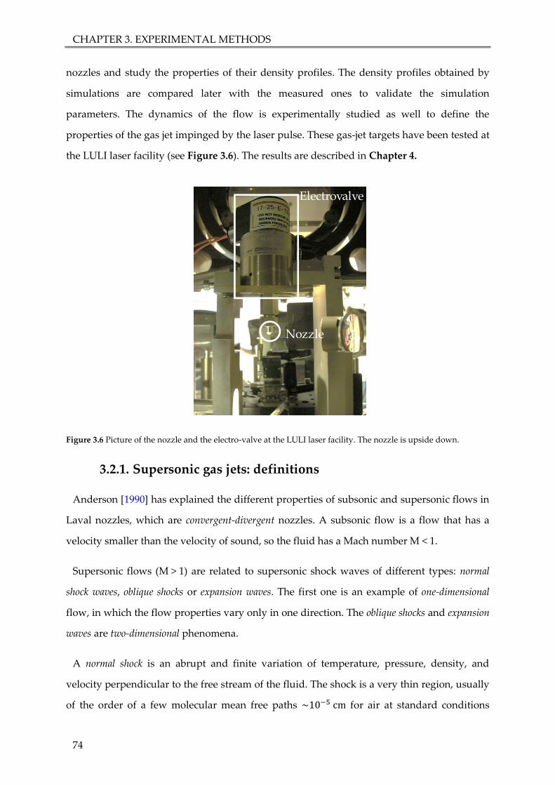
CHAPTER 3. EXPERIMENTAL METHODS
74
nozzles and study the properties of their density profiles. The density profiles obtained by
simulations are compared later with the measured ones to validate the simulation
parameters. The dynamics of the flow is experimentally studied as well to define the
properties of the gas jet impinged by the laser pulse. These gas-jet targets have been tested at
the LULI laser facility (see Figure 3.6). The results are described in Chapter 4.
Figure 3.6 Picture of the nozzle and the electro-valve at the LULI laser facility. The nozzle is upside down.
3.2.1. Supersonic gas jets: definitions
Anderson [1990] has explained the different properties of subsonic and supersonic flows in
Laval nozzles, which are convergent-divergent nozzles. A subsonic flow is a flow that has a
velocity smaller than the velocity of sound, so the fluid has a Mach number M < 1.
Supersonic flows (M > 1) are related to supersonic shock waves of different types: normal
shock waves, oblique shocks or expansion waves. The first one is an example of one-dimensional
flow, in which the flow properties vary only in one direction. The oblique shocks and expansion
waves are two-dimensional phenomena.
A normal shock is an abrupt and finite variation of temperature, pressure, density, and
velocity perpendicular to the free stream of the fluid. The shock is a very thin region, usually
of the order of a few molecular mean free paths ~10−5 cm for air at standard conditions
Nozzle
Electrovalve

3.2 Targetry: development of gas-jet targets
75
(273 K and 1 bar). A simple diagram of a normal shock is presented in Figure 3.7, taken from
[Anderson 1990]. When M1 and M2 are equal to 1, the normal shock is infinitely weak and it is
defined as a Mach wave.
Figure 3.7. Diagram of a normal shock. From [Anderson 1990].
Oblique shocks and expansion waves occur when supersonic flows bend their trajectories due
to a change in the surface direction. Diagrams of these two types of shocks are presented in
Figure 3.8, figure also taken from [Anderson 1990].
Figure 3.8. Diagrams of supersonic flow over a corner. From [Anderson 1990].
In Figure 3.8a, at point A, the slope of the surface changes by an angle 𝜃. Hence, the flow
streamlines are deflected upwards, following the surface direction. An oblique shock is formed
in the free-stream direction. Across the oblique shock, the Mack number decreases and the
pressure, temperature, and density increase. The weak oblique shocks correspond to Mach
waves in a two-dimensional flow.
In the case of a convex corner, Figure 3.8b, the flow streamlines are deflected downward,
towards the surface. The change of flow direction takes place across an expansion wave

CHAPTER 3. EXPERIMENTAL METHODS
76
centered at point A. Basically, the expansion wave is a continuous succession of Mach waves.
In contrast with the oblique shock, the flow properties change smoothly and continuously. The
M value increases and the pressure, temperature, and density decrease. If the convex corner
is sharp, the expansion fans are called centered or Prandtl-Meyer (who first worked out a
theory for this supersonic flow).
These different kinds of flows are at play in supersonic nozzles. A nozzle is a duct with a
throat connected at its inlet to a very large reservoir with total reservoir pressure 𝑝𝑟. (Figure
3.9a). The exit of the duct has an exit static pressure 𝑝𝑒. As 𝑝𝑒 is gradually reduced from 𝑝𝑟,
air flows from the reservoir to the exit with a mass flow �̇�. The mass flow through any
elemental surface arbitrarily oriented in a flowing fluid is defined �̇� = 𝜌 𝒖 𝒅𝑺, where 𝜌 is the
density, 𝒖 the velocity and 𝒅𝑺 = 𝒏 𝑑𝑆 where 𝒏 is the unit vector normal to the surface 𝑆. As
𝑝𝑒 is reduced, �̇� increase, until it remains constant even if 𝑝𝑒 is reduced all way to vacuum
(Figure 3.9b). The local Mach number increases through the convergent portion of the
nozzle, reaching the minimum area with a 𝑀 = 1, a sonic flow. When �̇� no longer increases
with the reduction in 𝑝𝑒, the duct is called to be choked. As the flow achieves the sonic flow in
the throat, in the convergent portion nothing happens.
Figure 3.9 a) Diagram of a nozzle, considering a duct with a throat, connected at its inlet to a very large reservoir
with total pressure 𝑝𝑟. The exit static pressure is defined as 𝑝𝑒 and the mass flow as �̇�. b) �̇� is presented as a
function of 𝑝𝑒. As 𝑝𝑒 decreases, �̇� increases. Until the duct is chocked and the mass flow no longer increases. The
figure was taken from [Anderson 1990].
When the exit pressure is reduced below the level required to reach choking, a new flow
emerges which is called the Laval nozzle flow. In the divergent duct, the flow becomes
supersonic, its velocity increases, the pressure decreases as the area increases.
A normal shock is formed inside the duct. As the exit pressure is reduced, the normal shock
wave moves downstream, closer to the nozzle exit. Behind the shock, the flow is subsonic, its
Mach number decreases, and density, temperature, and static pressure increase as we
a) b)

3.2 Targetry: development of gas-jet targets
77
observed in Figure 3.7. The shock produces a total pressure loss and the Mach number
behind the shock is lower than what they would be.
If the exit pressure is low enough, the exit flow becomes fully supersonic as the shock can
be moved outside the duct. There are three types of exit flows: over-expanded, Matched and
under-expanded, depending on the exit pressure 𝑝𝑒 and the back pressure 𝑝𝐵 of the
surrounding air. The first type, over-expanded flow, is when 𝑝𝐵 > 𝑝𝑒: the flow must adjust to a
higher pressure, see Figure 3.10a. An oblique shock attached to the nozzle exit is formed but
outside the duct. The second type of flow, Matched, is when 𝑝𝐵 = 𝑝𝑒 and the duct nozzle flow
comes out at the same pressure and no turning takes place in Figure 3.10b. The third one,
under-expanded flow, is when 𝑝𝐵 < 𝑝𝑒 and the nozzle flow must expand to match 𝑝𝐵 (Figure
3.10c). In this case, the flow is equilibrated due to expansion waves outside the nozzle.
A fourth type, more complicated than the others, is the jet shock diamonds, a combination of
under-expanded and over-expanded nozzle flows (see Figure 3.10d). The gas jet is propagating
through the atmosphere, which has boundary surfaces. Several oblique shocks are produced,
and their reflections at the boundaries are characteristic of this flow. The various reflected
waves form a diamond-like pattern.
Figure 3.10 Scheme representation of the flow of a) an over-expanded nozzle, b) a matched nozzle, c) an
under-expanded nozzle and d) a jet shock diamond. In this last picture, only the nozzle exit is presented on the left.
Taken from [Anderson 1990].
a) b)
c) d)

CHAPTER 3. EXPERIMENTAL METHODS
78
This is a quasi-one-dimensional consideration and it does not tell anything about the contour
of the duct. For real supersonic nozzles, the shock depends on the wall shapes, the thermal
conduction, the viscosity and so on. E.g. oblique shocks can occur inside the nozzle. We are not
going to describe in detail the numerical techniques for a steady supersonic flow, however,
Figure 3.11 shows a schematic of supersonic nozzle design in a two-dimensional
consideration.
Figure 3.11 Schematic of a supersonic nozzle design in two dimensions. From [Anderson 1990].
In the expansion section of the nozzle, expansion waves are generated and propagate. The
solid lines present the weak expansion waves, i.e., the Mach waves. Multiple reflections are
observed from the nozzle throat to the exit of the nozzle. We can observe that due to the
geometry symmetry, the waves generated from the top wall seems to be reflected from the
centerline. That is why the calculation can be simplified and one can only calculate the flow
above the centerline.
Figure 3.12 Density, static pressure, temperature, velocity, and Mach number obtained at the center of a helium
gas flow through a Laval nozzle obtained from computational fluid dynamics simulations from [Schmid 2012].

3.2 Targetry: development of gas-jet targets
79
Figure 3.12 shows the behavior of the different flow properties of a simulated
under-expanded nozzle. The figure is taken from [Schmid 2012]. It is possible to observe how
the M number (flow velocity) increases and it is equal to 1 at the throat of the nozzle
(light-blue dashed line). Meanwhile, the density (red solid line), the static pressure
(dark-blue dashed line), and the temperature (black dashed line) decrease from the reservoir
to the nozzle exit.
In this thesis work, three types of supersonic micrometric nozzles have been designed:
conical nozzles, shock nozzles, and asymmetrical nozzles. In Figure 3.13, a 3D presentation of
these nozzles is made with an artistic program [Sketchup]. The simplest one is the conical
nozzle, close to the Laval nozzle. This nozzle is modified with an edge at its exit to form a shock
nozzle (Figure 3.13b).
Figure 3.13 3D presentation of different types of nozzles. a) convergent-divergent nozzle similar to the Laval
nozzle: conical nozzle. b) Divergent-convergent nozzle with an edge at the exit of the nozzle: shock nozzle. c) A more
complex nozzle as a rectangular one: asymmetrical nozzle.
In the laboratory conditions, these nozzles produce under-expanded flow at the exit of the
nozzle. The edge of the shock nozzle produces a thin peaked density profile at a certain
distance of the nozzle exit due to the formation of oblique shocks. Its fabrication is not simple,
and the edge increases the manufacturing cost of the nozzle.
More complex nozzles can be interesting, e.g., asymmetrical nozzles. They may have
rectangular shapes at the throat and exit but the convergent-divergent shape is still present.
It is also possible to have one side convergent-divergent and the other convergent-straight
(see Figure 3.13c) and so on. As shock nozzles, their fabrication is more difficult and more
expensive than conical nozzles. Moreover, the non-axisymmetric nozzle experimental
Shock Conical Asymmetrical
a) b) c)
Gas
flow
z
x y x
z z

CHAPTER 3. EXPERIMENTAL METHODS
80
characterization is more complex (see Section 3.2.6). 3D CFD simulations, which are
extremely time-consuming, are needed.
3.2.2. Study and optimization of nozzle geometric parameters
In this thesis work, gas jets with an electronic density of around 1021 cm-3 are developed.
As seen in Chapter 2, the lasers are mostly absorbed around their critical densities. Such high
densities can be achieved with supersonic gas jets. The objective is to obtain a high density at
a certain distance from the nozzle exit under vacuum conditions, while controlling other
parameters such as the gas-jet divergence, transversal density profile, and longitudinal
shape. A proper understanding of the nozzle geometry is essential because it strongly
impacts the conditions mentioned above. E.g., the maximum density variation depends the
inlet pressure, exit nozzle diameters, and throat diameters. CFD simulations have been
performed to design different kinds of nozzles.
FLUENT simulations numerically solve the Navier-Stokes equations [Constantin 1988] on a
discrete grid. An implicit density-based coupled solver (DBCS) is used with double-precision
accuracy green-Gauss node-based gradients of solution variables, to solve the stationary fluid
flow, using a real-gas Peng-Robinson solution. The standard k-omega model is used to model
the turbulence [Wilcox 2006]. For symmetric nozzles, a 2D axisymmetric grid with
quadrilateral cells has been employed, which typically consists of 2 × 10⁵ cells with 2 × 10⁻²
average skewness ratio and minimum orthogonal quality of 8.5 × 10⁻¹. The grid is adapted
to the surfaces and it has been verified that further refinements do not change the simulation
results.
The nozzle is composed of a reservoir, a convergent section, a throat, and an expansion
section giving to a chamber under vacuum. The geometrical parameters of the simulation are
the throat diameter d, the nozzle exit diameter D, and the cone length L. Figure 3.14a shows
all these parameters. For shock nozzles, the length of the edge is denominated as E, as one can
see in Figure 3.14b. To facilitate the reading of this chapter, a schematic drawing of the
nozzle with its parameters is included as a foot note in some pages.
The simulation also takes into account a wall roughness of about 1 µm, that micrometric
nozzles machined by electroerosion usually show. The boundary conditions of the

3.2 Targetry: development of gas-jet targets
81
simulation are a high pressure at the inlet and two low pressures at the outlets in the vacuum
chamber outside the nozzle. The distance from the nozzle exit is represented by z. The
medium is diatomic hydrogen unless otherwise indicated.
Figure 3.14 Scheme of the 2D axisymmetric nozzle geometries for a) conical nozzles and b) shock nozzles used in
CFD simulations (see text for details).
The density evolution as a function of the reservoir pressure (or inlet pressure), 𝑝𝑟, is well
known to fit a linear progression [Couperus 2016]. Figure 3.15 shows the linear evolution of
the density as a function of the 𝑝𝑟 for three conical nozzles exit sizes D in the pressure range
between 50 and 1000 bar at a distance of z = 500 μm from the nozzle exit. This range of
pressures can be achieved with commercial gas boosters. In order to provide a bigger density
than the critical one, the minimum reservoir pressure is 400 bar. A 𝑝𝑟 of 1000 bar allows to
access a density close to the critical density almost independently of the nozzle parameters
and over-critical densities can be reached with optimized geometries. 𝑝𝑟= 1000 bar is chosen
to work with and optimize the nozzles with respect to their density profiles and shapes.
Figure 3.15 Evolution of the molecular density as a function of the reservoir pressure at a distance of 500 μm from
the conical nozzle exit for different exit sizes (400 μm, 450 μm and 500 μm).
inle
t
ou tlet
ou
tlet
L
d/2
D/2
Vacuum
chamber
rese
rvo
ir
z
Symmetry axis
r
inle
t
ou tlet
ou
tlet
L
d/2
D/2
Vacuum
chamber
rese
rvo
ir
z
Symmetry axis
r
Ea) b)
x
z

CHAPTER 3. EXPERIMENTAL METHODS
82
The laser-gas-jet interaction must take place at a certain distance z from the nozzle exit,
where the wanted density profile is achieved. z should be large enough to minimize the
nozzle damage during the laser-plasma interaction.
Conical nozzles
A detailed study is carried out to design conical nozzles capable to deliver more than
1021 cm−3 of diatomic hydrogen far from the nozzle exit. In order to find the optimum
parameters, density contour maps are made. The distance from the nozzle exit z is presented
as a function of the exit size D for different values of d and L.
Figure 3.16 Interpolated contour maps of the molecular density at 1000 bar of hydrogen at different distances
from the nozzle exit z as a function of the exit size D for three throat diameters (L is fixed) a) d = 100 µm, b)
d = 200 µm and c) d = 300 µm.
Figure 3.16 shows density contour maps comparing three throat diameters d = 100 µm,
200 µm, and 300 µm. The exit size D was varied from 100-200-300 µm to 450-550-650 µm
respectively. Distances z from the nozzle exit, z = 0, up to 650 μm by 50 μm steps are
investigated. For each figure, L = 1 mm is fixed while D is scanned.
A given density can be reached using different couples of exit sizes D and different
distances to the nozzle z. We can compare the three images and observe that a larger throat
diameter d induces an increase of the molecular density 𝜌 and a decrease of the optimum
distance from the nozzle, 𝑧. Some of the results are summarized in Table 3.1.
d D
L
a) d = 100 µm b) d = 200 µm c) d = 300 µm

3.2 Targetry: development of gas-jet targets
83
d = 100 µm d = 200 µm d = 300 µm
D = 300 µm
𝜌 = 4.4 × 1020 cm−3
z = 600 µm
𝜌 = 3.2 × 1021 cm−3
z = 300 µm
𝜌 = 1.1 × 1022 cm−3
z = 100 µm
Figure 3.16a Figure 3.16b Figure 3.16c
Table 3.1 Molecular densities, 𝜌, and the optimum interaction distances from the nozzle exit, z, achieved for a
nozzle exit D = 300 µm and different d values.
Figure 3.17 shows the FWHM contour maps performed with the same parameters as in
Figure 3.16. One observes that the maximum density corresponds to the minimum FWHM as
a result of the converging waves.
Figure 3.17 The FWHM interpolated contour maps at 1000 bar of hydrogen at different distances from the nozzle
exit z as a function of the exit size D for three throat diameters (L is fixed) a) d = 100 µm, b) d = 200 µm and
c) d = 300 µm.
We can compare the three images and observe that a larger throat diameter d induces an
increase of the FWHM and a decrease of the optimum distance from the nozzle, 𝑧. Some of
the results are summarized in Table 3.2.
d = 100 µm d = 200 µm d = 300 µm
D = 300 µm
𝐹𝑊𝐻𝑀 = 230 µm
z = 600 µm
𝐹𝑊𝐻𝑀 = 200 µm
z = 300 µm
𝐹𝑊𝐻𝑀 = 257 µm
z = 100 µm
Figure 3.17a Figure 3.17b Figure 3.17c
Table 3.2 FWHM and the optimum interaction distances, z, achieved for a nozzle exit D = 300 µm and different d
values.
a) d =100 µm b) d =200 µm c) d =300 µm
d D
L

CHAPTER 3. EXPERIMENTAL METHODS
84
In Table 3.2, the FWHM for d = 100 µm is larger than the one d = 200 µm. This is because
D = 300 µm is not an optimized value for a small throat diameter. For example, for
D = 150 µm a FWHM of 110 µm can be achieved.
Figure 3.17 also represents the divergence of the flow for a chosen exit size D value. We can
observe from Figure 3.17a that a further distance from the nozzle exit, z, induces an increase
of the FWHM. Some of the results are summarized in Table 3.3. A study of the gas jet
longitudinal profile is made further in Section 3.2.3.
D = 200 µm z = 200 µm z = 300 µm z = 400 µm z = 500 µm
d = 100 µm
Figure 3.17a 𝐹𝑊𝐻𝑀 = 140 µm 𝐹𝑊𝐻𝑀 = 170 µm 𝐹𝑊𝐻𝑀 = 270 µm 𝐹𝑊𝐻𝑀 = 370 µm
Table 3.3 FWHM achieved for a throat diameter d = 100 µm and nozzle exit D = 200 µm at different z values.
The exit size, D, dependence can be observed in Figure 3.16 and Figure 3.17. Comparing
the two images we observe that a larger nozzle exit D induces a decrease of the density, 𝜌, an
increase of the FWHM and an increase of the optimum distance from the nozzle, 𝑧. Some of
the results are summarized in Table 3.4.
D = 150 µm D = 250 µm D = 300 µm
d = 100 µm
Figure 3.16a
𝜌 = 3.8 × 1021 cm−3
𝐹𝑊𝐻𝑀 = 110 µm
z = 100 µm
𝜌 = 9.3 × 1020 cm−3
𝐹𝑊𝐻𝑀 = 170 µm
z = 350 µm
𝜌 = 4.5 × 1020 cm−3
𝐹𝑊𝐻𝑀 = 250 µm
z = 550 µm Figure 3.17a
Table 3.4 Densities, 𝜌, FWHM and the optimum interaction distances from the nozzle exit, z, achieved for a throat
diameter d = 100 µm and different D values.
Figure 3.18 shows the change of the density contour maps for different nozzle lengths L. In
the three images we observe that for different nozzle lengths L (in a small range between 1
and 3 mm), the density does not change dramatically. Some of the results are summarized in
Table 3.5.
However, if L is larger, Mach waves will dissipate inside the cone (see Figure 3.11) and a
shorter nozzle (< 0.5 mm) will not confine the flow, with a consequent decrease of density of
the gas jet produced and increase of its flow divergence [Schmid 2012].
d D
L

3.2 Targetry: development of gas-jet targets
85
Figure 3.18 Contour maps of the density at 1000 bar at different distances from the nozzle exit z as a function of
the exit size D for three lengths (d= 300 µm fixed): a) L = 1000 µm b) L = 2000 µm and c) L = 3000 µm.
z = 250 µm L = 1000 µm L = 2000 µm L = 3000 µm
D = 350 µm 𝜌 = 5.6 × 1021 cm−3
Figure 3.15a
𝜌 = 5.5 × 1021 cm−3
Figure 3.15b
𝜌 = 5.4 × 1021 cm−3
Figure 3.15c
Table 3.5 Densities achieved at z = 250 µm for a nozzle exit D = 350 µm and different L values.
Shock nozzles
The shock nozzle exit flow is different from the conical nozzle one because of its edge at the
nozzle exit. The other nozzle parameters are the same as in the previous case (throat
diameter d, exit diameter D, and cone length L) with the addition of an edge of length E. This
edge acts as a concave corner, forming an oblique shock at a fixed distance in the longitudinal
direction (z-axis). In this section, density flow side view images are presented to optimize the
nozzle parameters to reach the furthest interaction point.
The first parameter studied is the throat diameter, d (see Figure 3.19). D (480 µm) and E
(200 µm) are fixed. An increase of d induces an increase of the density and of the focal spot
size. This behavior has been already observed with conical nozzles, however, for shock nozzles,
we avoid the term FWHM and introduce the term focal spot size. This will be explained in
Section 3.2.3. In Figure 3.19, we can also observe how the shock formation distance, 𝑧𝑠ℎ𝑜𝑐𝑘,
decreases with the throat size. These results are summarized in Table 3.6. For the following
parameters, d will be fixed at 100 µm. This is the minimum diameter possible that
electroerosion can produce.
a) L = 1000 µm b) L = 2000 µm c) L = 3000 µm
d D
L
d D
L E

CHAPTER 3. EXPERIMENTAL METHODS
86
Figure 3.19 Molecular density maps at 1000 bar of hydrogen for different throat diameters d. The longitudinal
position is normalized to z = 0 at the exit of the nozzles. a) d = 100 µm, b) d = 200 µm and c) d = 300 µm. The red
color at the entrance of the nozzle can represent molecular densities larger than 1 × 1021cm−3.
d = 80 µm d = 100 µm d =120 µm
𝑧𝑠ℎ𝑜𝑐𝑘 ≃ 960 µm 𝑧𝑠ℎ𝑜𝑐𝑘 ≃ 840 µm 𝑧𝑠ℎ𝑜𝑐𝑘 ≃ 750 µm
Figure 3.19a Figure 3.19b Figure 3.20c
Table 3.6 Optimum interaction distances, 𝑧𝑠ℎ𝑜𝑐𝑘, achieved for D = 480 µm, E = 200 µm and different d values.
The second parameter studied is the exit diameter D, as observed in Figure 3.20. d (100 µm)
and E (150 µm) are fixed. When the exit diameter increases, the shock is created further from
the nozzle exit (the results are summarized in Table 3.7), and the density and the size of the
focal spot are decreased.
We can analyze the edge E variation, keeping d = 100 µm, D = 500 µm fixed. Figure 3.21
shows how a larger edge induces a focal spot area closer to the exit of the nozzle. These
results are summarized in Table 3.8. The dimensions of the spot size and density are
increased.
d = 80 µm
d = 100 µm
d = 120 µm
a)
b)
c)
d D
L E

3.2 Targetry: development of gas-jet targets
87
Figure 3.20 Molecular density maps at 1000 bar for different exit diameters D. The longitudinal position is
normalized to z = 0 at the exit of the nozzles. a) D = 460 µm, b) D = 480 µm and c) D = 520 µm. The red color at the
entrance of the nozzle can represent densities larger than 1 × 1021cm−3.
D = 460 µm D = 480 µm D = 520 µm
𝑧𝑠ℎ𝑜𝑐𝑘 ≃ 770 µm 𝑧𝑠ℎ𝑜𝑐𝑘 ≃ 840 µm 𝑧𝑠ℎ𝑜𝑐𝑘 ≃ 920 µm
Figure 3.20a Figure 3.20b Figure 3.20c
Table 3.7 Optimum interaction distances, 𝑧𝑠ℎ𝑜𝑐𝑘, achieved for d = 100 µm, E = 150 µm and different D values.
Figure 3.21 Molecular density maps at 1000 bar for different edge size E. The longitudinal position is normalized
to z = 0 at the exit of the nozzles. a) E = 180 µm, b) E = 220 µm and c) E = 250 µm. The red color at the entrance of
the nozzle can represent densities larger than 1 × 1021cm−3.
E = 180 µm E = 220 µm E = 250 µm
𝑧𝑠ℎ𝑜𝑐𝑘 ≃ 920 µm 𝑧𝑠ℎ𝑜𝑐𝑘 ≃ 845 µm 𝑧𝑠ℎ𝑜𝑐𝑘 ≃ 800 µm
Figure 3.20a Figure 3.20b Figure 3.20c
Table 3.8. Optimum interaction distances, 𝑧𝑠ℎ𝑜𝑐𝑘, achieved for d = 100 µm, D = 500 µm and different E values.
D = 480 µm
a)
b)
c)
D = 460 µm
D = 520 µm
a)
b)
c)
E = 180 µm
E = 220 µm
E = 250 µm
d D
L E

CHAPTER 3. EXPERIMENTAL METHODS
88
If only the nozzle length, L, varies, fixing D = 350 µm and d = 100 µm, the distance at which
the shock is formed and its density do not drastically change (see Figure 3.22).
Figure 3.22 Molecular density maps at 1000 bar for different nozzle lengths L with D and d constant. The
longitudinal position is normalized to z = 0 at the exit of the nozzles. a) L = 600 µm nozzle length, b) L = 800 µm
nozzle length and c) L = 1000 µm nozzle length. The red color at the entrance of the nozzle can represent densities
larger than 1 × 1021cm−3.
Asymmetrical nozzles (AN)
Asymmetrical nozzles require 3D simulations. Some have been performed, but their
computational cost did not allow a detailed study. The interest of asymmetrical nozzles is to
provide with a single nozzle two different transversal target profiles for laser interaction.
These are shown in Section 3.2.6.
Remark concerning the gas reservoir design
The nozzle geometrical parameters are essential for finding the optimum density profile.
However, one cannot forget about the design of the gas reservoir. As explained in Paper I, an
occasional formation of a supersonic flow section inside the transport system can generate
instabilities in the flow that lead to turbulences and flow-blocking zones. Figure 3.23
compares the effect of a conical transition (a) and a sharp transition (b). A sharp transition
leads to a perturbed flow propagation in the subsequent sections of the nozzle. The flow is
blocked and mass conservation cannot be reached due to the instabilities of the fluid flow.
The general rule is to avoid relatively big gas reservoir areas before the nozzle throat, to use
L = 1000 µm
L = 800 µm
L = 600 µma)
b)
c)
d D
L E

3.2 Targetry: development of gas-jet targets
89
conical profiles between sections of different diameters, to avoid sharp discontinuities or
surface irregularities and to propagate the flow from big diameters to lower diameters.
Figure 3.23 Effect of the sharp discontinuity in the converging region on the turbulent viscosity factor. The figures
represent half of the axisymmetric nozzle view where the lower line is the revolution axis. The inlet is in the left
and the outlet is in the right of each figure: a) a 59° convergent cone and b) a 90° transition.
3.2.3. Transversal and longitudinal density profiles
The gas-jet transversal density profile is fundamental to optimize the laser-driven ion
acceleration. Figure 3.24a shows conical nozzles density profiles with molecular densities up
to ~ 1 × 1021 cm−3 (it is assumed that all hydrogen atoms are ionized by the laser pulse,
therefore the free electron density is twice the molecular density) at z ≥ 200 µm. The FWHM
at a distance of the nozzle exit from z = 300 to 400 µm is less than 150 µm.
Figure 3.24 Transversal density profiles at 1000 bar for different distances from the nozzle exit z a) conical nozzles
b) shock nozzles. A comparison of both can be found in Figure 3.25b in logarithmic scale.
For further distances, the densities drop down to 4 × 1020 cm−3 and the FWHM increase.
For smaller distances, the densities are higher, but the profiles become flat-tops. Flap-top
a) b) Conical nozzle Shock nozzle
a) b)

CHAPTER 3. EXPERIMENTAL METHODS
90
profiles can be inhomogeneous depending on how the Mach waves converge and can
present dips or wavy structures. In the region of space where Mach waves converge,
Gaussian-like profiles with a minimum FWHM are found [Schmid 2012]. In this case, the
optimal distance is z = 400 µm.
Figure 3.24b shows the density profile for shock nozzles. It is important to notice how the
transverse density profiles change drastically with z. The optimum distance from the exit of
the nozzle is 𝑧 = 912 μm with a molecular density of 1.1 × 1021 cm−3. However, only 12 μm
below the density drops to 4.5 × 1020 cm−3 and the profile shape is lost. In this particular
case, the density profile is formed by the combination of a Gaussian background due to the
flow propagation and a sharp peak that stands over it due to the shock formation. The
Gaussian background forms two wings in both sides of the sharp peak. From the center of the
transversal density profile, the wings start before 100 μm with a molecular density of around
2 × 1020 cm−3 and continues even further than 500 μm with a molecular density
of 1019 cm−3. This is why we avoid the use of FWHM to characterize the density profiles of
this type of nozzles.
Figure 3.25 a) Comparison of the downstream propagation of the flow from the nozzle exit for shock nozzles and
conical nozzles. b) Comparison of both transversal density profiles in logarithmic scale at the optimal z where
maximal density is reached.
In Figure 3.25a, the comparison between both nozzle longitudinal density profiles is
presented. The shock nozzle shock converges further than the conical nozzle ones. For shock
nozzles, the achievement of the same density but at a further distance from the exit nozzle is
its main advantage. Before the converging point, the longitudinal density profile is different,
i.e., while conical nozzle density decreases with z, shock nozzle density slowly decreases until
a) b)

3.2 Targetry: development of gas-jet targets
91
there is an abrupt change and the density increases in several µm (at the shock nozzle focal
point). That is why the transversal profile presented in Figure 3.24b changes dramatically
with z. After the shock, the density decreases faster than in the conical nozzle case.
The comparison of the transverse density profiles is shown in Figure 3.25b. The shapes of
these density profiles are different, i.e., even if the reached maximum density is similar, one
must notice that the wings of shock nozzles are higher.
In the experiment, a laser pulse will first interact with the wings. If the density of the wings
is too high, the laser pulse may not be able to penetrate and interact with the high-density
peak as it will lose all its energy during this first interaction. From Figure 3.25b one can
observe that the interaction with the laser starts at least 100 µm before in the case of shock
nozzles compared with conical nozzles.
3.2.4. Remark concerning gas jets in air
During the experiment, the gas jets are always under vacuum (e.g. 𝑝𝐵 = 10−3-10−7 mbar)
and their flow propagation is under-expanded (Section 3.2.1). However, if there is an
increment of pressure in the chamber, the supersonic jet becomes over-expanded. The behavior
of an over-expanded jet is experimentally observed in Figure 3.26 with the designed conical
nozzles. After the first oblique shock, the pressure increases and there is a typical behavior of
diamond jet flows [Section 3.2.1].
Figure 3.26 Mach waves generated by the designed conical nozzle fed with a) 10 bar and b) 20 bar of nitrogen
propagating through 1 bar air. Mach waves are formed at different distances and propagate until they collapse.
a) b)
Nozzle Nozzle
3 mm 3 mm

CHAPTER 3. EXPERIMENTAL METHODS
92
Figure 3.27 Propagation in air at 1 bar pressure for Mach waves generated by the designed conical nozzle fed with
50 bar N2 a) measurement and b) simulation. Shock fronts are observed in both cases at the same distance of the
nozzle exit.
Shock fronts are reproduced by simulations with an inlet pressure of 50 bar of nitrogen (see
Figure 3.27). The nozzle parameters are the same as the one used in the experiment and the
outside pressure is around 1 bar, the atmospheric pressure. The shock front is measured at
z = 1500-1700 µm (the error is due to the incertitude of the nozzle exit position) and the
simulation gives a shock front at 1620 µm. A good agreement between the experiment and
the simulation is observed.
3.2.5. Conclusion
In this section we recall the main conclusions of the parametrical study of the nozzle
geometries for conical nozzles and shock nozzles in Table 3.9.
Among all parameters, FWHM one is not easy to define for shock nozzle (which transversal
profile is not a Gaussian distribution). If one characterizes the shock nozzles with the FWHM
of the sharp profile edge, the wings contribution is neglected, and this is a problem since it
plays a major role in the laser-matter interaction. Thus, for shock nozzles, we prefer to talk
about the spot size defined by the entire density profile.
The increase of d implies an increase of the maximum density and of the FWHM/spot size.
The focal distance decreases. A balance between the maximum density, small FWHM/spot
size, and far focal distance must be found.
a) b)
Nozzle Nozzle
3 mm
d D
L E
d D
L

3.2 Targetry: development of gas-jet targets
93
Conical nozzle Shock nozzle
d ↑
↑ 𝜌max
↑ FWHM / spot size
↓ z
D ↑
↓ 𝜌max
↑ FWHM ↓ spot size
↑ z
L ↑ ≈ z
≈ 𝜌max
E ↑ -
↑ 𝜌max
↑ spot size
↓ z
Table 3.9 Summary of the behavior of conical and shock nozzles with the different nozzle parameters. Note that d
is the throat diameter, D the nozzle exit diameter, L the cone length and for shock nozzles, E is the length of the
edge. 𝜌max is the maximum molecular density at the distance z from the exit of the nozzle.
An increase of D means a decrease in the maximum density. For conical nozzles, the FWHM
increases while for shock nozzles the spot size decreases and the focal point is further from the
nozzle exit.
A slide modification of L, if L ≃ 1 mm, does not play an important role.
Last, only for shock nozzles, an increase of E implies higher density, bigger focal spot size
and a closer shock formation from the exit of the nozzle.
We calculate the dependence on the focal distance of each parameter. We conclude that, for
conical nozzles, both parameters (d and D) have the same importance for the optimum focal
distance. For shock nozzles, the most critical parameters are E and D. These results are
summarized in Table 3.10.
Conical nozzles Shock nozzles
- 𝐸 [𝜇𝑚] = −0.58 𝑧 [𝜇𝑚] + 711
𝐷 [𝜇𝑚] = 0.34 𝑧 [𝜇𝑚] + 121 𝐷 [𝜇𝑚] = 0.4 𝑧 [𝜇𝑚] + 147
𝑑 [𝜇𝑚] = −0.39𝑧 [𝜇𝑚] + 332 𝑑 [𝜇𝑚] = −0.19 𝑧 [𝜇𝑚] + 260
Table 3.10 Dependence on the focal distance of each parameter.
d D
L
d D
L E

CHAPTER 3. EXPERIMENTAL METHODS
94
3.2.6. Experimental characterization of the gas jet
In order to validate the CFD simulations, the real density profile delivered by the gas-jet
conical nozzles is measured with a Mach-Zehnder interferometer using different gases. The
gas-jet flux dynamics are studied as well.
Mach-Zehnder interferometer
In Figure 3.28a, the scheme of the interferometer is presented. An overview can be seen in
Figure 3.29. The light radiation source of 20 mW Melles-Griot HeNe (632.8 nm) is employed
and a Kepler beam expander is installed to increase the beam diameter in order to cover all
gas-jet volume. With this configuration, it is possible to add a pinhole in its focus, which
spatially filters the laser beam, to remove noise from modes other than the Gaussian one and
to obtain a homogeneous beam. The system is formed by an 𝑓1 = 40 mm lens (N-BK7,
biconvex, 350-700 nm antireflection coated) and 𝑓2 = 200 mm lens (N-BK7, plano-convex,
633 nm coated) separated 240 mm, which gives a magnification of x5. The beam diameter is
0.96 mm at the entrance of the beam expander and at the exit is 4.8 mm. The spot size at
FWHM where the pinhole is placed is around 70 µm, and the pinhole is 75 µm of diameter.
Figure 3.28 a) Scheme of the Mach-Zehnder interferometer (red line). Strioscopy (blue line) is set up by blocking
the reference ray in the interferometer and by including a sharp object in the focus of the imaging lens. The signal
is detected by a photodiode. b) Interferogram obtained with N2 at 1000 bar reservoir pressure and c) density
reconstruction considering an axisymmetric nozzle.
a) b)
c)

3.2 Targetry: development of gas-jet targets
95
Figure 3.29 a) General view of the interferometer chamber, b) view from the inside of the chamber.
The laser beam is divided by a beamsplitter cube (BS) into reference and probe rays, with the
probe ray passing through the gas jet. The two laser beams are recombined by another BS to
obtain a phase shift image. BS are made to split and recombine the laser light between 420
and 680 nm. A halfwave plate is also installed to control the relative intensity of polarized
light that goes to each arm of the interferometer. The gas-jet nozzle is mounted on a
Clark-Cooper solenoid valve EX30 that can provide continuous or pulsed gas flux. The high
density is reached by using 1000 bar inlet pressure delivered by a Haskel gas booster model
AGT-62/152. A lens images the phase shift interferogram onto a linear CCD camera PixelFly
whose magnification allows to get approximately 3 microns/pixel. An 𝑓3 = 500 mm lens
(N-BK7, plano-convex, 633 nm coated) is used. The object is at 735 mm from the lens, giving
an image with an enlargement of x2.12 at around 1563 mm. The image has a size of ~10 mm.
The background noise of the interferometric image is reduced by subtracting the
reconstructed image without gas (unperturbed condition). A good shot-to-shot stability and
reproducibility is observed.
The phase shift induced by the gas flow is obtained by the fringe displacement from the
unperturbed position in vacuum (Figure 3.28b). A phase shift measurement allows the
reconstruction of the gas-jet density profile by means of the variation of the refractive index
n. Assuming a cylindrical symmetry of the gas jet (which is the case with axisymmetric
nozzles) the reconstruction of the density profile along one direction is possible from a
single-phase shift image (Figure 3.28c). The radial distribution of the refraction index is
deduced using Abel inversion. A description of the mathematical extraction of the phase
shift variation and the Abel inversion can be found in [Malka 2000]. The phase shift
a) b)
2nd BS nozzle
Solenoid
valve

CHAPTER 3. EXPERIMENTAL METHODS
96
calculation and the reconstruction of the density profile from the refractive index variation
are performed by the analysis program [Neutrino]. The gas molecule number density 𝜌 is
calculated from the general form of the Lorentz-Lorentz equation [Born 1999],
𝜌 =3
4𝜋𝛼
𝑛2 − 1
𝑛2 + 2 (3.1)
where α, the mean polarizability of the gas molecule, is defined as
𝛼 =3𝐴
4𝜋𝑁𝐴 (3.2)
where 𝐴 is the molar refractivity and 𝑁𝐴 is Avogadro’s number. Last two equations can be
combined to obtain
𝜌 =𝑁𝐴𝐴
(𝑛2 − 1)
𝑛2 + 2 (3.3)
The molar refractivities for hydrogen and nitrogen are calculated using the last equation
and refractive indices of gases from [Peck 1977] (see Table 3.11). It is known that they remain
constant even at high pressures when n differs from unity [Born 1999].
Hydrogen [m3/mol] 2.094 × 10⁻⁶
Nitrogen [m3/mol] 4.506 × 10⁻⁶
Table 3.11 Calculated values of molar refractivity of hydrogen and nitrogen using refractive index values from
[Peck 1977].
Experimental measurement of nitrogen molar refractivity is described in [Stone 2004]
giving a value of 4.445 × 10⁶ m3/mol. With this value and the one calculated for hydrogen
(no experimental value was found), the density profiles are reconstructed in Figure 3.30.
Due to the opacity of the gas jet at high densities, reconstruction of the density is only
possible in a moderate-density region (1019 - 1020 cm−3). For this reason, the measurements
are performed away from the exit of the nozzle (z > 500 µm). The density profiles obtained
by interferometry (blue solid line) are compared to the ones obtained by CFD simulations

3.2 Targetry: development of gas-jet targets
97
(red dashed line) with diatomic hydrogen at 50 bar and 100 bar, and diatomic nitrogen at 100
and 1000 bar.
Figure 3.30 Comparison of simulation results with interferometry reconstructions for a) 50 bar diatomic hydrogen
at z = 750 µm b) 100 bar diatomic hydrogen at z = 750 µm c) 100 bar diatomic nitrogen at z = 500 µm d) 1000 bar
diatomic nitrogen at z = 1000 µm.
The fluctuations in the central region of the profiles are artifacts due to the inherent noise of
the Abel inversion close to the axis of symmetry and the imprecision of the symmetry axis
position. The overall good agreement validates our simulations and gives us confidence in
their results at 1000 bar with diatomic hydrogen.
The hydrogen interferogram is more difficult to obtain due to its small refractive index
(1.0001493) compared to the one of nitrogen (1.0002984) [Peck 1977]. That is why the
fluctuations obtained with hydrogen are bigger (See Figure 3.30).
3D tomography
3D characterization by tomography is needed for nozzles without cylindrical symmetries
(e.g. asymmetrical nozzles). Abel inversion is no longer possible in those cases and this
complicates the characterization process. To measure the density profile of a non-cylindrical
nozzle, several images of the phase shift displacement have to be taken at different angles
b)
a)
c)
d)

CHAPTER 3. EXPERIMENTAL METHODS
98
(see Figure 3.31). This study was made with nitrogen at 100 bar. This step can be developed
with neutrino. In our case, a rotation plate is placed around the nozzle to allow the
acquisition of phase shift images at controlled angles.
Figure 3.31 Images of the phase shift taken at different rotation angles with asymmetrical nozzles. These pictures
are produced with [Neutrino] and the phase shift is normalized to one.
Figure 3.32 Reconstruction of the phase shift at 200 µm of the asymmetrical nozzles exit with TomoRaw program.
a) Using one iteration series between each pair of images b) Using two interaction series and a mask to avoid the
erroneous interferences of the reconstruction from the overlapping borders. Both images are normalized to 1.
Each phase-shift matrix from each angle is normalized and used as input into a
tomographic reconstruction code (TomoRaw) developed at LULI. It extracts the matrices
between each measure by different iteration series. To precisely measure the density profile
at all angles, a high quantity of images is needed. In our case, as a motorized rotation plate
was not available, images for only 7 angles are taken. Figure 3.32 shows the reconstruction of
40˚ 60˚ 90˚ 105˚
135˚ 150˚ 180˚
a) b)
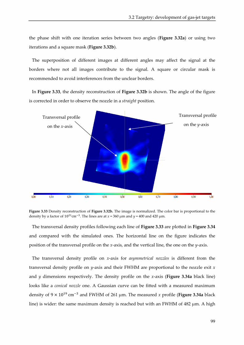
3.2 Targetry: development of gas-jet targets
99
the phase shift with one iteration series between two angles (Figure 3.32a) or using two
iterations and a square mask (Figure 3.32b).
The superposition of different images at different angles may affect the signal at the
borders where not all images contribute to the signal. A square or circular mask is
recommended to avoid interferences from the unclear borders.
In Figure 3.33, the density reconstruction of Figure 3.32b is shown. The angle of the figure
is corrected in order to observe the nozzle in a straight position.
Figure 3.33 Density reconstruction of Figure 3.32b. The image is normalized. The color bar is proportional to the
density by a factor of 1021cm−3. The lines are at x = 360 µm and y = 400 and 420 µm.
The transversal density profiles following each line of Figure 3.33 are plotted in Figure 3.34
and compared with the simulated ones. The horizontal line on the figure indicates the
position of the transversal profile on the x-axis, and the vertical line, the one on the y-axis.
The transversal density profile on x-axis for asymmetrical nozzles is different from the
transversal density profile on y-axis and their FWHM are proportional to the nozzle exit x
and y dimensions respectively. The density profile on the x-axis (Figure 3.34a black line)
looks like a conical nozzle one. A Gaussian curve can be fitted with a measured maximum
density of 9 × 1019 cm−3 and FWHM of 261 µm. The measured x profile (Figure 3.34a black
line) is wider: the same maximum density is reached but with an FWHM of 482 µm. A high
Transversal profile
on the y-axis
Transversal profile
on the x-axis

CHAPTER 3. EXPERIMENTAL METHODS
100
background is found on the x-axis line, which may explain why the measure and the
simulated FWHM differ.
Figure 3.34 Density profile measured by TomoRaw (black) and compared with FLUENT simulations (red) for
a) the transversal profile on the x-axis b) the transversal profile on the y-axis.
The simulated y profile matches with the measured one (Figure 3.34b). However, we
observe that the density at ± 250 µm is bigger in the case of the experimental results.
Dynamics of the gas jet
During the experiment, a solenoid valve is used to produce pulsed gas jets. Perfect
characterization of the dynamics of the gas flux is mandatory to synchronize it with the
incoming laser pulse. The goal is to trigger the laser interaction when the maximum density
of the gas jet is reached. The evolution of the gas flow is measured by strioscopy (based on
the Schlieren effect). Strioscopy is an optical Fourier process in which the light diffused from
an object is filtered by an obstacle and the diffracted light is measured (Figure 3.28a). The
refractive index gradient of the object deflects the light in different optical path lengths and
the turbulences generated by the density gradient can be detected with a photodetector
[Hirschberg 2002]. This method allows finding the precise moment of flow stabilization for
different gases, pressures, and opening time durations of the solenoid valve.
In Figure 3.35a, c and e, one can see the gas flow evolution for different opening time
durations. The rising time of the gas jet corresponds to the time needed to completely fill the
nozzle reservoir volume (about 230 mm3), and it is also affected by the size of the throat
(100 mm). The time needed to reach the maximum density may be reduced using smaller
a) Transversal profile on the x-axis b) Transversal profile on the y-axis

3.2 Targetry: development of gas-jet targets
101
reservoirs. The dimension of the reservoir and throat also affect the time needed to
completely evacuate the gas once the solenoid valve is closed. In the following work,
mechanical constraints related to the solenoid valve did not allow to reduce the reservoir
size.
Figure 3.35 Gas flow evolution of a) b) diatomic hydrogen c) d) diatomic nitrogen e) f) helium as a function of time
for a) c) e) different solenoid valve opening durations b) d) f) different pressures. When the solenoid valve is
triggered (at t = 0 ms) is about 12 ms before the gas flow.
Figure 3.35a shows the diatomic hydrogen flow dynamics for different valve opening
durations. For the experiment, it is important to achieve the maximum density with the
a) b)
c) d)
e) f)

CHAPTER 3. EXPERIMENTAL METHODS
102
minimum quantity of gas in the vacuum chamber. The maximum of the density for diatomic
hydrogen gas jet is reached after a time = 70 ms with a larger valve opening duration of
𝑡𝑜𝑝𝑒𝑛 = 40 ms. To minimize the gas quantity in the vacuum chamber, this time should be
carefully chosen. In the case of diatomic nitrogen, the gas flow takes time = 110 ms to reach
the maximum density with a larger valve opening duration 𝑡𝑜𝑝𝑒𝑛 = 80 ms (Figure 3.35b). The
dynamics of nitrogen is slower than the one of hydrogen, and more gas flows inside the
vacuum chamber. This is due to the different gas molecular weights. For helium gas, the
strioscopy and interferometry are more complicated to perform because of its smaller
refraction index (1.000036 vs 1.000149 for hydrogen gas [Peck 1977]). The stabilization takes
place at time = 70 ms for an opening duration of 𝑡𝑜𝑝𝑒𝑛 = 40 ms.
For the three gases, a comparison of the flux dynamics with the inlet pressure is made
(Figure 3.35b, d, and f). As observed with the FLUENT simulations, the gas-jet density
evolution as a function of the inlet pressure displays a linear progression (Figure 3.15).
However, one observes that the stabilization time does not depend on the reservoir pressure.
Figure 3.35b shows the flux evolution for hydrogen gas for an opening duration of
𝑡𝑜𝑝𝑒𝑛 = 20 ms. Even if this is not the optimum opening duration, the maximum density is
achieved at the same time, time = 57 ms at all reservoir pressures. The linear progression can
be obtained again with the maximum densities (maximum density [a.u.] = 0.0051 reservoir
pressure [bar] + 1.32).
Figure 3.35d shows the nitrogen flux dynamics for an opening duration of 𝑡𝑜𝑝𝑒𝑛 = 80 ns.
The maximum density is reached at time = 110 ms for all pressures as well. In this case, the
equation is maximum density [a.u.] = 0.0104 reservoir pressure [bar] + 0.89. It is still linear but
the slope has a different value. The constant factor is not relevant, as the measurements are
not done with the same exact conditions from one gas to the other.
Figure 3.35f presents the case of helium for an opening duration, 𝑡𝑜𝑝𝑒𝑛 = 30 ms. The time at
which the maximum density is reached is 68 ms. As mentioned above, strioscopy
measurements are more difficult to perform with helium, so the flux dynamics cannot be
compared in height between the different pressures since the experimental conditions had to
be modified during the measurements.

3.3 Particle and X-ray diagnostics
103
3.3. Particle and X-ray diagnostics
The laser interaction with a target generates different radiations and accelerates electrons
and ionized particles. There are several ways to detect ionizing particles and these can be
divided into two groups: one based on passive detectors and the other one on active
detectors. In experimental setups, these detectors can be used alone or as parts of more
complex systems, e.g. spectrometers. In this section, the most common detectors and
spectrometers are described. With them, it is possible to characterize the energy, number,
and the divergence of the accelerated ion/electron beams, or X-ray spectra.
3.3.1. Passive detectors
Three types of passive detectors are mostly used: Columbian resin #39 (CR-39) films,
radiochromic films (RCF), and imaging plates (IP). They are 2D detectors without magnetic or
electric fields. They are not sensitive to electromagnetic noises, unlike electronic devices.
They are mostly used in stacks to analyze the ion beam energy distribution and its
divergence. In this thesis, RCF and IP were used as passive detectors.
Radiochromic films (RCF)
These films consist of a single or double radiation-sensitive layer on a thin polyester base
with a transparent coating. The RCF are sensitive to ionizing particles under which their
active layer (dye) turns from white to blue. The resulting optical density is directly related to
the absorbed dose. The advantage of this simple detector is that no complex processing is
required since they are easily readout with standard scanners. However, for quantitative
analysis, it is important to allow the chemical reaction in the sensitive layer to take place
during some hours after their irradiation and scan them afterwards with the scanner used for
their calibration and using the same digitalization parameters (resolution, wavelengths and so
on). The resulting digitized maps of optical density are translated into energy deposits in the
films using dose to optical density (OD) response functions. 𝑂.𝐷. = - log (𝐼𝑡/𝐼𝑟𝑒𝑓) where 𝐼𝑡 is
the intensity transmitted by the irradiated RCF and 𝐼𝑟𝑒𝑓 the reference intensity transmitted
by a virgin film. The modification of the optical density is proportional to the deposited dose
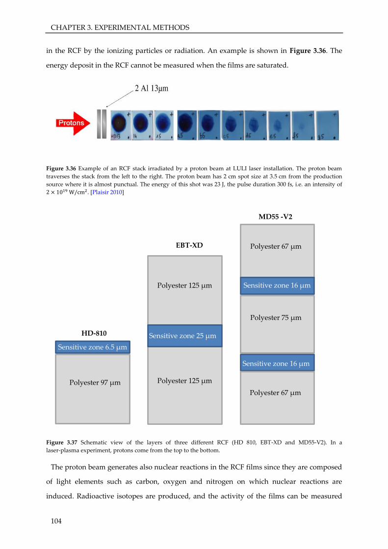
CHAPTER 3. EXPERIMENTAL METHODS
104
in the RCF by the ionizing particles or radiation. An example is shown in Figure 3.36. The
energy deposit in the RCF cannot be measured when the films are saturated.
Figure 3.36 Example of an RCF stack irradiated by a proton beam at LULI laser installation. The proton beam
traverses the stack from the left to the right. The proton beam has 2 cm spot size at 3.5 cm from the production
source where it is almost punctual. The energy of this shot was 23 J, the pulse duration 300 fs, i.e. an intensity of
2 × 10¹⁹ W/cm2. [Plaisir 2010]
Figure 3.37 Schematic view of the layers of three different RCF (HD 810, EBT-XD and MD55-V2). In a
laser-plasma experiment, protons come from the top to the bottom.
The proton beam generates also nuclear reactions in the RCF films since they are composed
of light elements such as carbon, oxygen and nitrogen on which nuclear reactions are
induced. Radioactive isotopes are produced, and the activity of the films can be measured
Sensitive zone 6.5 µm
Polyester 97 µm
Polyester 67 µm
Sensitive zone 16 µm
Sensitive zone 25 µm HD-810
MD55 -V2
Polyester 67 µm
Sensitive zone 16 µm
Polyester 75 µm
Polyester 125 µm
Polyester 125 µm
EBT-XD

3.3 Particle and X-ray diagnostics
105
and studied. Hence the proton beam properties (energy distribution and number of particles)
can be inferred from the activities measured in the RCF stack [Plaisir 2010].
Several types of films have been manufactured by GafchromicTM and each type of film has
a different composition (HD-810, EBT, MD-55 …) with different updates (MD-55-V2, EBT1-3,
… , EBT-XD). E.g. HD-810 films have one sensitive zone of 6.5 µm thickness. EBT-XD films
contain a 25 µm layer between two polyester layers of 125 µm. MD-55-V2 films consist of
two sensitive layers of 16 µm each (see Figure 3.37). These last films are more sensitive than
the first ones.
Imaging plates (IP)
IP are detectors sensitive to ionizing radiation and particles, e.g., photons, electrons, and
ions. After irradiation, these films must be processed by a scanner. A spatially resolved 2D
image is obtained, in which the content of each pixel (or intensity) is related to the number of
electron-holes (metastable states) created in the film by the ionizing radiation. They can be
reused as white light recombines the formed electron-holes. They are more sensitive than
RCF and their good spatial resolution (25 µm) makes them good detectors for spectrometers
such as Thomson parabolas (TP) (see Section 3.3.3).
Fuji Photo Film Co. Ltd provides three different types of IP: BAS-SR, BAS-MS and BAS-TR.
They have up to four different layers: protective, sensitive, support, and magnetic layer. The
ionizing particles traverse the IP from the protection layer to the magnetic one. Both BAS-SR
and BAS-MS films have a 6 and 9 µm protective layer respectively which stops protons with
energies lower than 600 keV, while BAS-TR films are protective layer-free. The sensitive one
for BAS-MS and BAS-TR is composed of BaFBr0.85I0.15: Eu2+ of 115 and 50 µm respectively
and the support one of C2H20 of 190 and 250 µm thicknesses respectively. The magnetic layer
is ZnMn2Fe5NO40H15C10 and have 160 µm thickness. These values are summarized in Table
3.12.
The physics process inside an IP has been presented by H. von Seggern [1992]. An ionizing
particle traverses the sensitive layer and forms an electron-hole, ionizing the dopant Eu2+.
The electron is captured by the FBr- or the FI- to form a metastable complex. The information
of the ionizing particle is stored as number of electron-holes. The deexcitation can occur

CHAPTER 3. EXPERIMENTAL METHODS
106
spontaneously, by a process called fading. On the other hand, the recombination can be
stimulated by photons. This last process is interesting to measure the IP signal. The
stimulated recombination generates a photostimulated luminescence photon (PSL) (see Figure
3.38). It can be by electron transport in the valence band or by tunnel effect if the FBr- or the
FI- are close to the Eu3+. The deexcitation by fading is a loss of information. That is why the IP
must be scanned as soon as possible after the irradiation [Bonnet 2013].
SR MS TR
Protection
Composition C2H20 -
Thickness [µm] 6 9
Sensitive
Composition BaFBr: Eu2+ BaFBr0.85I0.15: Eu2+
Thickness [µm] 120 115 50
Support
Composition C2H20
Thickness [µm] 188 190 250
Magnet
Composition ZnMn2Fe5NO40H15C10
Thickness [µm] 160
Table 3.12 Composition and thickness of the different layers in SR, MS and TR imaging plates.
During the experiment, IP were analyzed using a FUJIFILM FLA-7000 reader after each
shot. They were scanned ~20´ after the laser-matter interaction. The fading can be neglected in
these conditions [Bonnet 2013]. The scanner has a laser wavelength optimized for FBr- or FI-
stimulation and a photomultiplicator that counts the luminescence photons. Once the
measurement is done, it is possible to delete the information in the IP by using intense white
light. After 5´ the films are erased and can be reused. After irradiation with the signal to be
measured and before placing the IP in the scanner, they must not be exposed to light, so
every manipulation is to be done in darkness. The scanner generates a matrix with numerical

3.3 Particle and X-ray diagnostics
107
values per pixel which are coded in 2 octets (quantum level (QL)). Each QL from each IP pixel
is converted to PSL by the function:
𝑃𝑆𝐿 = (𝑅𝑒𝑠
100)2 400
𝑆 10
𝐿(𝑄𝐿2𝐷−1
−12) (3.4)
where PSL is the photostimulated luminescence photons in one pixel, Res is the resolution (size
of a pixel), S the sensibility, L the latitude, D the lecture dynamic (8 or 16 bits) and QL the
numerical value of the pixel (from 0 to 2𝐷 − 1). In our case, the resolution was 50 µm, the
sensibility 4000, the latitude 5 and it was coded on 16 bits.
Figure 3.38 Levels of BaFBr crystal doped with Europium in the SR IP sensitive layer. The figure is taken from
[Bonnet 2013].
3.3.2. Active detectors
More complex detectors, but important for HRR experiments, are 2D electronic detectors
that provide short (few seconds) readout times. Fast scintillators coupled to a CCD or a
photomultiplier tube (PMT), a micro-channel plate (MCP) coupled to a phosphor screen and
complex CCD are examples of active detectors (e.g. for plasma images or X-rays detection).
Recently, diamond detectors are also being used in laser-plasma experiments.
The detection acquisition time can be optimized to discriminate signals produced by
protons, ions, electrons and X-rays. The signal from electrons is usually suppressed by
magnetic fields placed in front of the detector entrance.
Conduction band
Valence band

CHAPTER 3. EXPERIMENTAL METHODS
108
Scintillators
A scintillator is a material that produces light when it is excited by ionizing radiation. The
material may absorb the particle energy and scintillate, or if metastable excited state are
populated, the light produced by the deexcitation of the electrons from the excited states to
lower states is delayed from the input signal.
Sometimes the scintillator is coupled to an electronic light sensor (PMT, photodiode or
silicon photomultiplier). The PMT absorbs the light emitted by the scintillator and generates
electrons by the photoelectric effect. The multiplication of electrons amplifies the input signal
and results in an electrical signal that can be analyzed.
In addition, nuclear techniques can be useful for particle characterization. Tarisien et al.,
designed and built the nuclear activation technique for analysis of laser induced energetic particles
(NATALIE) system [Tarisien 2011]. It can quantify precisely laser-accelerated particles by
simultaneous counting several activated samples. NATALIE is a set of 32 NaI scintillator
detectors assembled in pairs that measure the two 511 keV coincident photons following a
nuclear β+ decay. This system can be operated for particle energies above a few MeV up to
several tens of MeV with very accurate measurement of the energy and angular distribution
of the particle beams.
Micro-channel plate (MCP)
An MCP is a 2D detector that amplifies electron signal in several million of channels which
act as independent electron multipliers, as presented in Figure 3.39. If an ionizing particle
enters into a channel and hits its walls, electrons are emitted and accelerated by the electric
field generated by a high voltage applied on both sides of the MCP (In our case, -2000 V).
These electrons are multiplied until a cascade emerges from the rear of the plate. The
electrons then are attracted by the +5000 V of the phosphor plate placed at some mm away
from the MCP. The phosphor is excited and generates light in some ms. An image can be
taken by a CCD placed behind the phosphor.
The operation of an MCP is not straightforward, e.g. in the case of needed manipulation in
air, a maximum time of 2h is recommended since little dust affects the measurement of the
signal. However, HRR ion beam characterization is possible with this kind of detector,

3.3 Particle and X-ray diagnostics
109
problems with breakdowns between Thomson parabola (TP) electrodes are less important than
in the IP case and the detection efficiency is high.
Figure 3.39 Schematic of a microchannel plate (MCP) detector. At the left, a single channel electron multiplier. At
the right, with electron multiplication dynamics [dm photonics].
CCD
In all laboratories, common CCDs are used for optical alignment of laser beams or even
coupled to an MCP. They have good resolutions for small prices.
More complex cameras are used for X-ray detection. E.g., in this thesis, a deep-depletion
X-ray CCD was used (model PI-LCX:1200 cooled with liquid nitrogen) to detect X-rays
produced by the interaction of protons and photons with a sample. The quantum camera
efficiency extended above 20 keV, allowing us to count X-ray photons around 8 keV. A thin
beryllium window is always present to seal the deep cooling, protect de CCD from visible
light and reduce the background (more information is given in Chapter 5).
Diamonds
Chemical vapor deposition (CVD) diamonds are wide-bandgap intrinsic semi-conductors that
have outstanding intrinsic properties such as low leakage currents, fast time response or
radiation hardness. The energy of a charged particle is deposited in the material creating a
free electron-hole pair (energy gap = 13.6 eV). A voltage is applied to the electrodes of the
detector to allow the charged particle collection. The voltage amplitude is chosen such to
have an electric field E > 1 MV/m in order to operate in electron holes pairs velocity
saturation regime. Their radiation hardness allows them to tolerate high radiation doses
without degradation of their properties. The energy necessary to create a free electron-hole
pair guarantees a very low dark current and prevents IR and visible light from contributing

CHAPTER 3. EXPERIMENTAL METHODS
110
to the signal. Their small sizes make them interesting for laser-driven acceleration
experiments. There are two different electrodes configuration of CVD diamond detectors:
planar or transverse. [Verona 2015]. Both structures are presented in Figure 3.40.
Figure 3.40 Two different types of electrodes layout: a) the interdigital configuration, b) sandwich configuration.
They are both mounted inside a cylindric metallic enclosure designed to minimize the EMP effects. [Verona 2015]
These types of detectors have been developed and optimized together with a readout
system to operate in critical environments (laser-plasma interaction ones) [Marinelli 2013,
De Angelis 2016]. At the ALLS installation thanks to the contribution of M. Salvadori [2020],
two CVD diamond detectors were used for proton time of flight (TOF) measurements. Both
have an active layer of thickness 50 µm grown on a commercial 4×4×0.5 mm high pressure
high temperature (HPHT) substrate but are presenting two different electrode layouts. The
signal collected by the CVD diamond detector is sent to a Tektronix DPO 7104 scope (1 GHz
bandwidth and 5 Gs/s sample rate) through 15 m long RG 223 cables. The detectors are
triggered by a signal correlated to the laser pulse arrival on target. They are shielded for a
good reduction of the EMP noise which affects all the electronic devices placed nearby the
experimental chamber.
3.3.3. Spectrometers
Spectrometers are useful tools to measure the number of ions as a function of their energy.
In laser-plasma experiments, the TOF and TP spectrometers are commonly used. While the
TOF cannot distinguish different ion species, TP allows splitting and steering the ions to
separate the contribution of each ion species and its energy.
a)
b)

3.3 Particle and X-ray diagnostics
111
Time of flight (TOF)
A TOF spectrometer consists of a long vacuum tube connected to a detector. Ion beams can
spread out temporally because of the velocity dispersion. It is simple and has fast readout for
HRR lasers. However, no distinction between different ions is possible. Other particles, e.g.
electrons, can be easily deviated by small magnets.
The detector can be a plastic scintillator placed far (several meters) from the interaction
point. The protons arrive at different times at the scintillator depending on their energy. The
scintillation light is converted into electrons by a photocathode and multiplied by a PMT.
The signal is read by an oscilloscope. However, the signal of the PMT is not linear which
makes impossible the measurement of the absolute number of protons with different
energies. Moreover, the scintillator must be placed far away from TCC to have a good
resolution (see Figure 3.41).
Figure 3.41 The first ALLS configuration. TOF line coupled with an PMT at 0˚. On the left, at 45˚, the TP
spectrometer.
The replacement of the plastic scintillator by a diamond is interesting because of its fast
response. The diamond detector can be closer to the interaction point and still have a good
time resolution, even if there is no possibility to split the different accelerated ions.
Moreover, diamond detectors have a small size which is always an advantage (e.g. there is
the possibility of using several detectors in the same chamber).
PMT
TOF line @ 0˚ TP @ 45˚

CHAPTER 3. EXPERIMENTAL METHODS
112
This type of spectrometer was used at EMT-INRS center in a second configuration and they
were placed in almost symmetrical positions (-6 and +9 degrees). In Figure 3.42, it is possible
to see the experimental chamber with the KF40 pipes leading to the diamond detectors.
Figure 3.42 Second ALLS configuration: TOF lines at -6˚ and 9˚. One can observe the small size of the diamond
detectors. The line in the middle is for the TP (@ 0˚).
Thomson parabola (TP)
TP is a useful spectrometer: it is capable to disperse, in energy and in mass-to-charge
(A/Z) ratio, different ion species. A traditional TP scheme is shown in Figure 3.43. It consists
of pairs of rectangular magnets and electrodes that produce uniform magnetic and electric
fields respectively. A particle passes through the magnetic and electric field and its trajectory
is steered by the Lorentz force (𝑚𝒂 = 𝑞(𝑬 + 𝒗 × 𝑩)). The electric and magnetic fields are
parallel to each other and perpendicular to the ion initial momentum. The particle trajectory
is deviated as a function of its energy by the magnet in the longitudinal axis and then
deflected as a function of its A/Z ratio in the vertical axis by the electric field. If particles have
different energies, a parabola is formed for each ion species.
Figure 3.43 Schematic of a Thomson parabola TP spectrometer. 𝐿𝐵1 and 𝐿𝐸1is the magnet and electric plates
length and 𝐿𝐵2 and 𝐿𝐸2 the distance from the magnet or the electric plates to the detector.
TOF 9°
TOF -6°
Particle
Pinhole MagnetsElectric plates
Detector
LB1 LB2
LE2LE1

3.3 Particle and X-ray diagnostics
113
TP are usually shielded (e.g. by lead walls) for signal-to-background ratio improvement
and equipped with pinholes at their entrances for better energy resolution.
Considering uniform electric and magnetic fields without fringe field effects, the ion
displacement at the detector for non-relativistic cases along the vertical direction (Y, as the
electric field) and horizontal direction (X, as the magnetic field) is:
𝑋 = 𝛼𝐵 (𝐿𝐵12
2+ 𝐿𝐵1𝐿𝐵2)
(3.5)
𝑌 = 𝛼2𝐸𝑚
𝑞(𝐿𝐸12
2+ 𝐿𝐸1𝐿𝐸2)
Where 𝛼 = 𝑞/𝑚𝑣𝑧 and 𝑣𝑧 is the longitudinal speed of the ion (of mass m and charge q) at
the pinhole, 𝐿𝐵1, 𝐿𝐵2, 𝐿𝐸1, 𝐿𝐸2 correspond to the distance shown in Figure 3.43, and E and B
are the electric and magnetic field strengths, respectively. The distance X and Y are derived
using equations of motion for the particles and the Lorentz force neglecting the change of 𝑣𝑧.
More information in [Gwynne 2014].
The displacement has a linear dependence on the magnetic (B) and electric (E) field
strengths and a stronger dependence on the length of the magnets and electric plates. Since
electrons have an opposite charge compared to protons, they are deflected inside the
magnetic field in the opposite direction.
Figure 3.44 Scanned BAS-TR IP that shows the three different parabolas from the helium-hydrogen gas mixture
used as a target. The spot at the left indicates the initial position of the particles before being deflected by the
electric and magnetic fields. The X-rays and UV light from the laser reach the IP at this spot.
For the gas-jet experiments, TP were used coupled to IP. Figure 3.44 shows a scanned
BAS-TR IP after the PICO2000 laser interaction with a helium-hydrogen mixture gas-jet
target. The parabolas from protons (H+), and helium ions (He++and He+) are shown on the

CHAPTER 3. EXPERIMENTAL METHODS
114
right. The spot on the left indicates the initial position of the particles before being deflected.
For the analysis, once the logarithmic response of the detector (QL) is linearized (PSL)
[Dorias 2015], one must sum vertically the PSL of a parabola trace (e.g, the one for protons).
An example is shown in Figure 3.45. For each ion species, a parabola trace and a background
trace were isolated, and the background was carefully subtracted. In the case of several
parabolas, the maximal energy may be probably underestimated because of parabola trace
overlaps.
Figure 3.45 Making the assumption that the parabola trace is just in 10x10 pixels (represented as squares) a) QL
must be converted in PSL before any manipulation. b) Then one can sum the PSL for each column.
The conversion PSL position to energy can be calculated with the TP geometry and/or its
magnetic field map. All TP used during the experiment campaigns have been calibrated in
energy at the AIFIRA accelerator facility at CENBG, in the energy range from 500 keV to
3.5 MeV. Figure 3.46 shows the PSL position as a function of the energy.
Figure 3.46 Four different ion beam energies were analyzed in AIFIRA accelerator. 0.7 MeV, 1 MeV, 2 MeV and
3 MeV. A fit was done to relate the position of the beam spot to its energy. This process was performed for all the
TPs used in the gas-jet experiment.
QL
PSL
a) b)

3.3 Particle and X-ray diagnostics
115
The number of protons at each pixel position (or ion energy) is extracted from the number
of PSL using the response functions shown in Figure 3.47 taken from [Bonnet 2013].
However, before using this response function, one must check if the scanner conditions are
similar to the one use in [Bonnet 2013]. The number of protons/MeV/sr is obtained dividing
the number of protons by the solid angle of the parabola pinhole (in steradian) and by the
value of the energy bins in the spectra.
Figure 3.47 Response function R(E) of BAS-MS, BAS-SR, and BAS-TR IPs. The symbols represent the data from
[Bonnet 2013]. For more information [Bonnet 2013].
The uncertainties in the energy value and in the number of protons/MeV/sr (Np/MeV/sr)
were calculated assuming that all variables (solid angle 𝛺, response function, number of
PSL, energy calibration) are statistically independent and summing their variances.
𝑁𝑝/𝑀𝑒𝑉/𝑠𝑟 =𝑁𝑝
Ω𝐸
{
𝑁𝑝 =
𝑠𝑖𝑔𝑛𝑎𝑙𝑁𝐵𝑁𝑝−𝑃𝑆𝐿
=𝑠𝑖𝑔𝑛𝑎𝑙𝑇 − 𝑠𝑖𝑔𝑛𝑎𝑙𝐵
𝑁𝑝−𝑃𝑆𝐿
Ω =𝜋 (𝜙2)
2
𝑑𝑇𝐶𝐶2
𝐸 = 𝑑𝑖𝑓𝑓(𝐸)
(3.6)
where 𝑁𝑝/𝑀𝑒𝑉/𝑠𝑟 is the number of protons/MeV/sr, 𝑁𝑝 the number of protons, 𝑠𝑖𝑔𝑛𝑎𝑙𝑇 the
signal obtained in the IP detector, 𝑠𝑖𝑔𝑛𝑎𝑙𝐵 the background signal, 𝑠𝑖𝑔𝑛𝑎𝑙𝑁𝐵 the actual signal
with background subtracted, 𝜙 the pinhole diameter, 𝑑𝑇𝐶𝐶 the distance from the target to

CHAPTER 3. EXPERIMENTAL METHODS
116
the pinhole, 𝐸 the energy binning. As the uncertainties are statistically independent, the
total uncertainty can be calculated as:
𝛿𝑁𝑝−𝑠𝑟 ≈ |𝑁𝑝−𝑠𝑟| (𝛿𝑁𝑝𝑁𝑝
+𝛿Ω
Ω+𝛿𝐸
𝐸) (3.7)
The energy is measured with an accuracy of about 3%. The accuracy of Np/MeV/sr is
about 50% at low energies and about 20% at high energies.
Figure 3.48 Schematic of the TP-MCP used at the EMT-INRS center. The detector is in a different vacuum
chamber allowing a differential vacuum and the possibility of opening the main chamber without breaking the
vacuum in the detector chamber. The real photo is in Figure 3.49 [Paper III].
Figure 3.49 a) Picture of the detector chamber connected to the boule rouge at EMT-INRS center. b) Picture of the
CCD pointed at the MCP inside the detector chamber. The picture is taken under the black blanket on the right of
picture a).
The TP at the EMT-INRS was used with an MCP as detector ( Figure 3.48 and Figure
3.49). The TP-MCP is placed in a separate chamber in a high-quality vacuum. The TP was
calibrated in intensity on the 2x6 MV Tandem linear accelerator from University of
Montreal (UdM). A cross-calibration was performed between the TOFs and the MCP to
Detector chamber
Entrance pinhole
0.5 T permanent magnet
± 7 kV electrodes
MCP
Phosphor
CCD
Window
Objective
To computer
10-6 mbar 10-8 mbar
a) b)

3.3 Particle and X-ray diagnostics
117
calibrate the relevant parameter of the TP spectrometer required to find the proton kinetic
energy. More information about this calibration can be found in [Paper VII].
Figure 3.50 shows a typical MCP image obtained from the TP spectrometer with a Cu
target. One can see the parabola from the light species: protons, H+, and different carbon ion
species (C4+, C3+ and C3+ ). A less intense copper ion parabola is observed as well.
Figure 3.50 MCP image obtained from the TP spectrometer with a Cu target. Taken from [Paper VII].
The manipulation of the MPC is more complicated than the IP, however, they are suitable
for HRR. Moreover, breakdown problems are less important in the case of MCPs. Both
detectors are sensitive to UV so the breakdowns are detected. In the case of IP, the
breakdowns marked the IPs and they could not be used for that shot.


119
CHAPTER 4.
GAS TARGET EXPERIMENT RESULTS
4.1. Introduction
The designed gas-jet nozzles presented in Section 3.2 are tested in two different
experimental campaigns with the PICO2000 laser system. In the experiment, proton
acceleration is studied using hydrogen gas and different types of nozzles: big and small
conical nozzles, and asymmetrical nozzles. Shock nozzles were designed after the experiment. The
parameters of each type of nozzle are summarized in Table 4.1. Moreover, helium
acceleration is studied with a mix of hydrogen and helium gases using an asymmetrical
gas-jet target. These results are discussed in Section 4.4.
4.1. Experimental setup
Four TPs with their respective IP are used to detect and resolve in charge and energy the
accelerated ions. They are placed at 0°, 30°, 60°, 90° with respect to the laser axis in the first
campaign, and at 0°, 30°, 70°, 80° in the second campaign (Figure 4.1) due to space
constraints. They are shielded by lead walls for signal-to-background ratio improvement and
equipped with pinholes at their entrances for better energy resolution. The pinhole diameters
are smaller than 500 µm.

CHAPTER 4. GAS TARGET EXPERIMENT RESULTS
120
Big conical
nozzle
Small conical
nozzle 1
Small conical
nozzle 2 Asymmetrical nozzle
Shape Conical Conical Conical Rectangular
d [µm] 300 100 100 100 x 100
D [µm] 400 200 240 500 x 100
L [mm] 1 1 1 1
𝒛𝐨𝐩𝐭 [µm] 200 200 400 200
𝝆𝐦𝐚𝐱 [𝐜𝐦−𝟑] 3.54 × 10²¹ 1.53 × 10²¹ 8.95 × 10²⁰ 7.22 × 10²⁰ 4.31 × 10²⁰
FWHM [µm] 347 140 148 480 139
Table 4.1 Parameters of the nozzles used in the experiments (d is the throat diameter, D the nozzle exit diameter
and L the cone length). The optimal interaction distance 𝑧𝑜𝑝𝑡, the maximum molecular density delivered 𝜌𝑚𝑎𝑥 and
the FWHM of the density profile are given in the two last rows.
Figure 4.1 Experimental setup at the LULI facility. PICO2000 high-power laser is impinging on the high-density
gas-jet target. Four TPs equipped with IPs are placed at 0°, 30°, 70°, and 80° with respect to the laser axis, 50 cm
away from the gas-jet target.
x
y Laser transversal direction
Laser longitudinal direction
x z Gas jet flow direction
axis

4.2 Laser-beam alignment and plasma diagnostics
121
The gas-jet target alignment is achieved using bottom and side views placed in the
chamber. During the interaction, both views are also used as plasma detectors. The 2ω
emission in the interaction is recorded in the bottom view camera. During the second
campaign, 500 ps after each shot, a shadowgraphy picture is saved using the side view CCD.
4.2. Laser-beam alignment and plasma diagnostics
For the laser beam alignment, a tip at TCC is the reference (x = 0, y = 0 and z = 0). Figure
4.2a shows the laser shining on it. The red cross indicates TCC. In Figure 4.2b a nozzle is
placed at the same place. Its illumination and the magnification of the image were not
optimal in the first campaign, both parameters are improved in the following one (Figure
4.4).
Figure 4.2 First experiment bottom view. The red cross represents TCC. a) The illuminated tip at TCC. b) The
nozzle at the same place.
The same optical path is used to observe the second-harmonic (2ω) emission of the plasma
during the laser-gas interaction. In this case, a band-pass filter is placed in front of the CCD.
Second-harmonic generation is an important indicator of nonlinear laser-plasma interaction.
Its characteristics can provide information about e.g. the laser energy absorption
mechanisms. Images of second-harmonic generation induced by a ponderomotive force have
been presented in [Mori2002]. Stronger second-harmonic generation was observed in
[Zhizhan 1983; Stamper 1985]. It was usually due to self-focusing, filamentation or
stimulated Raman scattering. In this work, the laser ponderomotive force sweeps the
Shining tip at TCC
Nozzle exit at TCC
a) b)

CHAPTER 4. GAS TARGET EXPERIMENT RESULTS
122
electrons away from the laser beam path inducing a change of the refractive index which
may probably be at the origin of the 2ω emission.
In the experiment, the 2ω emission is observed when the laser interacts with the different
types of gas targets. Figure 4.3a and b show the 2ω emission from the bottom view for a big
conical nozzle and a small conical nozzle 1 respectively. Figure 4.3c shows the comparison of
the gas density profile of each nozzle at the interaction distance z = 200 µm. The laser is
always focused at TCC, as indicated on the figures with a red cross. The red arrows indicate
the laser direction, along the longitudinal position (x-axis). To modify the relative position
between the center of the nozzle and the laser focus, the nozzle is displaced in the laser’s
longitudinal position. In the picture, the grey circle indicates the position of the nozzle at the
time of the shot.
Figure 4.3 Capture of the 2ω emission of the plasma during 250 ps after the laser-gas interaction on a) a big conical
nozzle b) a small conical nozzle 1 . c) The gas density profile for these different types of gas targets.
Big conical nozzles SCN
1000 bar H2; z = 200 µm
a) b)
c)
Small conical nozzles 1
Laser

4.2 Laser-beam alignment and plasma diagnostics
123
With a big conical nozzle (see Figure 4.3a), even if the laser focus is planned at the entrance
of the nozzle, the generation of the second harmonic is observed before. That could mean
that the plasma in the wings of the gas density profile (Chapter 3) is too dense and the laser is
not capable to traverse it, i.e., the laser interacts with a plasma before the maximum density,
losing its energy. The interaction seems to start before x = - 600 µm from the focal point,
where the density of the plasma is of the order of 1019 cm−3 (see Figure 4.3c). The start of the
interaction was too far to be observed.
In the second case, for a small conical nozzle 1 (Figure 4.3b), the second-harmonic generation
is observed closer to the focal point. The density profile is thinner so the laser starts the
interaction closer to the nozzle entrance, at x ≃ -300 µm, where the density of the gas jet is
also about 1019 cm−3. The maximum signal is observed at the center of the nozzle exit.
Figure 4.4 Pictures from the bottom view CCD in the second experiment a) of the illuminated tip at TCC b) of the
nozzle at TCC. The red cross represents TCC.
Figure 4.5 Picture from the side view CDD. The nozzle is upside down.
Shining tip at TCC
Nozzle exit at TCC
a) b)
Nozzle shadow

CHAPTER 4. GAS TARGET EXPERIMENT RESULTS
124
In the second campaign, the resolution and illumination of the nozzles are improved
(Figure 4.2 vs. Figure 4.4). An additional CCD is placed at one side of the nozzle which is
used to observe the shadowgraphy of the plasma enligthed by a Quanta-Ray laser (ns)
(Figure 4.5). The precision of our alignment in the second campaign is therefore better.
Nozzles are always small conical nozzles 2 and the interaction point is at z = 400 µm from the
nozzle exit. In Figure 4.6a, the focus is made at the center of the gas jet while in Figure 4.6b
the laser is focused at the rising slope of the jet density profile. In both cases, the main
interaction at the focal point is observed. However, it is difficult to explain the different
shapes observed. Proton energy spectra from those shots are plotted in Figure 4.12b and
Figure 4.13a respectively.
Figure 4.6 Capture of the 2ω emission of the plasma during 120 ps after the laser-gas interaction on a conical
nozzle. a) The nozzle is placed at TCC b) The rising slope of the jet density profile is placed at TCC.
On the side view, the plasma expansion is recorded with a small conical nozzle 2. In Figure
4.7, a dense plasma (dark blue) is observed on both sides of the interaction point, at
z = 400 µm from the nozzle exit. This plasma expands and follows the rest of the gas. A dense
plasma is also formed at the surface of the nozzle. Nozzle damage was observed in both
campaigns after one laser shot. The nozzles were more damaged in the first campaign (when
the laser was focused 200 µm from the nozzle exit) compared to the second one (𝑧 = 400 μm).
As a consequence of this damage, in the experiment, the nozzles were changed after each
shot. We can conclude that, for no damage to the nozzle, much higher interaction distances
should be used.
a) b)Small conical nozzle 2 at TCC Small conical nozzle 2 at x = 72 µm

4.3 Results on proton acceleration
125
Figure 4.7 Shadowgraphy of the plasma by a Quanta-Ray laser (ns) during 500 ps after the laser-gas interaction.
4.3. Results on proton acceleration
4.3.1. 1st campaign
The first campaign objective is the study of different nozzle types (big conical nozzles, small
conical nozzles 1 and asymmetrical nozzles) to test the best design for ion acceleration. Most of
the shots are performed with hydrogen for protons acceleration. The detector used in the TP
is BAS-TR IP.
Firstly, proton acceleration is obtained using big conical nozzles. The laser is focused at
200 µm from the nozzle exit (in the z direction) and the nozzle is placed 150 µm away from
TCC in the x direction (for better understanding of the nozzle displacement, seen Figure
4.3a). The laser interacts with the gas-jet target 18 ms after the release of the gas. The
electro-valve allows the gas flow during 20 ms (𝑡𝑜𝑝𝑒𝑛 = 20 ms). During some shots, the effect
of the ASE on the proton spectra is studied. We modified the ASE level tuning the Pockels cell
delay (PD), as explained in Section 3.1.1.
Figure 4.8 shows typical spectra obtained with the laser (𝐸𝐿 ≈ 75 J) focused at the rising
slope of the gas-jet density profile and with the ASE level defined as PD = 0. The spectrum in
Figure 4.8a shows that about 1012 protons in a continuous energy distribution up to 1.5 MeV
are emitted in all directions. The signal in the laser’s transversal direction seems higher,
nozzle
y
z
plasma
shadow

CHAPTER 4. GAS TARGET EXPERIMENT RESULTS
126
however, micro breakdowns in the 90° TP introduce a big uncertainty on the number of
protons (± 80%). In Figure 4.8b, when the ASE was reduced to PD = 1.05 ns, higher energy
protons in the laser’s longitudinal direction (x-axis) are reported. Small second structures
(shown in red circles) at 2.8 MeV and 5 MeV at 0° are observed. At 30°, a second structure
(plateau) with a constant number of 1010 protons with energies from 1 MeV up to 2.5 MeV is
noticed. The ASE is more reduced in order to obtain a higher signal in the laser’s
longitudinal direction. However, the ASE is too reduced (PD = 1.25 ns, Figure 4.8c) and the
laser pulse wavelength spectrum starts to decrease; with the consequence of larger pulse
duration. The signal in the laser’s longitudinal direction is not improved. The relative delay
between the Pockels cells is then determined as 1.05 ns for the following laser-plasma
interactions with the minimum ASE level achievable.
Figure 4.8 Proton energy spectra at 0° (red), 30° (blue), 60° (green) and 90° (black) obtained with the laser focused
at the rising slope of the big conical nozzle density profile at z = 200 µm. The ASE is continuously reduced from one
shot to the other.
Proton acceleration is also achieved using small conical nozzles 1. The laser was focused at
200 µm and 250 µm from the nozzle exit (z-axis). The molecular density profiles are shown in
PD = 0 nsa) b)
c)
PD = 1.05 ns
PD = 1.25 ns
0˚ TP limit

4.3 Results on proton acceleration
127
Figure 4.9a. On the x-axis, the nozzle was placed 60 µm away from TCC. The laser interacts
with the gas-jet target 64 ms after the gas release (𝑡𝑜𝑝𝑒𝑛 = 30 ms).
First, the same interaction conditions are performed two times, with the small difference
that the laser energy on the target is 66.5 J in the first shot and 75.5 J in the second one. Figure
4.9b and c show about 1013 protons with energies up to 2.5 MeV at all angles but 30°. A good
repeatability is observed. Secondly, the interaction distance from the nozzle is modified, so
that the laser interacts with a different density profile. The spectra is shown in Figure 4.9d. A
thinner density profile seems to improve the acceleration in the longitudinal direction of the
laser.
Figure 4.9 Proton energy spectra at 0° (red), 30° (blue), 60° (green) and 90° (black) obtained with the laser focused
at the rising slope of the small conical nozzle 1 jet density profile at c) and d) 200 µm b) 250 µm. A comparison
between the density profiles at z = 200 µm and z = 250 µm is shown in a).
Protons are also accelerated using asymmetrical nozzles. The laser focus is at 200 µm from the
nozzle exit and the nozzle was placed at TCC. The laser interacts with the gas-jet target 64 ms
after its release (𝑡𝑜𝑝𝑒𝑛 = 30 ms). Two shots are done with this type of nozzle, with a possibly
a)
c) z = 250 µm; EL = 67 Jd)
z = 200 µm; EL = 66.5 J
z = 200 µm; EL = 75.5 J
b)

CHAPTER 4. GAS TARGET EXPERIMENT RESULTS
128
slightly different orientation for one to the other due to a bad bottom view resolution in the
first campaign. The corresponding gas density profiles are shown in Figure 3.24. Other
parameters are similar with a small difference in the laser energy (𝐸𝐿 = 66.5 J vs 75.5 J). In the
first shot, proton acceleration is mainly observed at 0° and 90° with a maximum energy of
2 MeV (Figure 4.10a). In the second shot, (Figure 4.10b) protons are more isotropically
accelerated. However, a peaked structure at 3.9 MeV is observed in the laser’s longitudinal
direction.
Figure 4.10 Proton energy spectra at 0° (red), 30° (blue), 60° (green) and 90° (black) obtained with the laser
focused at the rising slope of the asymmetrical nozzle jet density profile at z = 200 µm. The orientation is probably
different in figure a) and b).
In summary, proton acceleration with asymmetrical nozzles is interesting because
longitudinal acceleration to high energies (up to 4 MeV in Figure 4.10b) is obtained.
However, the alignment is not precise and the characterization as shown in Section 3.2.6 is
harder than for other nozzles. This is why we did not use this type of nozzle in the second
campaign. Comparing big and small conical nozzles 1, the maximum energy is similar, but
more protons are accelerated with small conical nozzles 1 (Figure 4.9). The laser cannot
penetrate into the gas target delivered by big conical nozzles due to its thick density profile, so
it does not interact with the target maximum density. This phenomenon was also observed
in Figure 4.3a, where we could see that, even if the laser focus was planned at the entrance of
the nozzle, the generation of the second harmonic was observed before. Moreover, more gas
is delivered into the vacuum chamber with the big conical nozzles which usually produced TP
breakdowns. The amount of background present on the IP, in this case, is therefore higher.
As a consequence, the statistical fluctuations of the spectra are bigger.
a) b) EL = 75.5 JEL = 66.5 J

4.3 Results on proton acceleration
129
4.3.2. 2nd campaign
In the 2nd campaign, we used only one type of nozzle, small conical nozzles 2, and we
improved the detection setup. As mentioned before, small conical nozzles are chosen because
they provide the biggest flux of protons with good repeatability, easy alignment, and
characterization. In order to improve the small conical nozzle 1 used in the first campaign and
try to avoid the nozzle damage, some modifications were performed to achieve a similar
density profile but at a further distance from the nozzle exit. 400 µm from the nozzle exit is
achieved. Moreover, BAS-MS IP are used as detectors, gaining one order of magnitude on
the background level. That is also why the signal at energies smaller than 0.7 MeV is not
present on the following spectra. Examples of proton spectra with BAS-TR and BAS-MS IPs
from Fuji Photo Film Co. Ltd are shown in Figure 4.11.
Figure 4.11 Proton energy spectra recorded at 30° in two similar shots using both types of IPs. The one in red is
from a BAS-TR IP while the black one is from BAS-MS IP. Dashed lines indicate the detection limit corresponding
to the mean value of the background level plus two times its variance.
BAS-TR IP display a background of (1.9 × 10⁹ ± 1.4 × 10⁹) protons/MeV/sr while for
BAS-MS IP it is (0.25 × 10⁹ ± 0.22 × 10⁹) protons/MeV/sr. This is probably due to their
different sensibility to UV light. Note that the energy is measured with an accuracy of about
3%. The accuracy of Np/MeV/sr is about 50% at low energies and about 20% at high energies.
Figure 4.12 shows typical spectra obtained with the laser focused at the center of the gas jet.
With no modification of the Pockels cell delay (PD = 0 ns, Figure 4.12a), ~1011 protons/MeV/sr
in a continuous energy distribution up to 1.5 MeV are observed in all directions. By reducing

CHAPTER 4. GAS TARGET EXPERIMENT RESULTS
130
the ASE at half of the minimum achievable (PD = 0.8 ns, Figure 4.12b) a second structure up
to 2.5 MeV is observed in the laser transverse direction containing 1010 protons/MeV/sr.
Unfortunately, the TP at 80° was not in place in some shots.
Figure 4.12 Proton energy spectra at 0° (red), 30° (blue), 70° (green) and 80° (black) obtained with the laser
focused at the center of the gas jet b) and reducing the ASE at half of the minimum achievable.
Figure 4.13 shows typical spectra obtained with the laser focused at the rising slope of the
gas-jet density profile. With and without modification of the ASE, about
1011 protons/MeV/sr in a continuous energy distribution up to 2 MeV are observed at 0° and
30°. A similar distribution in a larger energy range is also observed in the other directions
(70° and 80°). When the ASE is reduced (PD = 0.8 ns), the contribution of a second structure
from 2 MeV to 3 - 4 MeV is larger, containing 5 × 10¹⁰ protons/MeV/sr. Besides the
structures already presented, an additional peak at 2.3 MeV is observed at 0° in Figure 4.13a.
Figure 4.13 Proton energy spectra at 0° (red), 30° (blue), 70° (green) and 80° (black) obtained with the laser
focused at the rising slope of the jet density profile b) and the ASE is reduced.
a) b) PD = 0.8 nsPD = 0 ns
a) b) PD = 0.8 nsPD = 0 ns

4.3 Results on proton acceleration
131
In conclusion, the laser focus at the rising slope of the gas-jet density profile provides more
energic protons and even additional peaked structures.
It is worth noting that the angular position and energy of the peaked structure at 0° in
Figure 4.13a is highly dependent on the laser and target parameters. Small variations of these
(e.g., the lower maximum density of the gas jet and laser fluctuations) can shift the peak to
the transverse directions (70° and 80°) and to different energies (3.3 MeV), as seen in Figure
4.14. In Figure 4.14b, a clear plateau structure in the energy range 2-3 MeV is also observed
at 30°. Similar features in the laser transverse direction can be seen in Figure 4.15a or Figure
4.12b at 70°.
Figure 4.14 Proton energy spectra at 0° (red), 30° (blue), 70° (green) and 80° (black) obtained with the laser
focused at the rising slope of the jet density profile.
Figure 4.15a presents the proton energy distribution measured with the laser focused at the
rising slope of the gas-jet density profile and the ASE level reduced at minimum achievable.
The spectra display more complex structures. The proton flux at 80° is smaller than in
previous shots, while the maximum energy at 0° is higher. Three particular features can be
seen on the spectrum in the laser’s longitudinal direction. The proton flux drops from 1011 to
109 in the energy range between 0.5 MeV and 2 MeV. Then it increases up to 1010 between
1.7 MeV and 3 MeV and the third peak with a flux of 5 × 10⁹ is observed in the range of
4.3 MeV to 5.3 MeV. Another peak at the energy of 3.4 MeV can also be seen at 70°. Figure
4.15b presents the proton energy distribution with a worse contrast. This time the complex
structures appear at 30° up to 5 MeV of energy.
a) b)

CHAPTER 4. GAS TARGET EXPERIMENT RESULTS
132
Figure 4.15 Proton energy spectra at 0° (red), 30° (blue), 70° (green) and 80° (black) obtained with the laser
focused at the rising slope of the jet density profile and the ASE level was reduced at the minimum achievable.
These results are discussed in the following section, 4.3.3, and compared with
hydrodynamics and PIC simulations.
4.3.3. Hydrodynamic and PIC simulations
PIC simulations with the PICLS code are used for interpretation of the measured proton
spectra. The PICO2000 laser parameters at normal incidence and s-polarization are utilized
as inputs (Section 3.1.1). The temporal and spatial laser intensity profiles are described by
truncated Gaussian functions. The laser temporal pulse is truncated at 2 ps. The pulse is
injected at the left side of the simulation box (600 × 160 µm2) at a time t = 0. Assuming that
the high-intensity laser pulse fully ionizes the gas; the target is described as a 380 µm length
plasma of electrons and protons. The mesh size is 80 nm and 15 particles of each species are
used in each cell. Physical processes are simulated during 3.6 ps with a time step of 0.267 fs.
Absorbing boundary conditions for the fields and the particles are applied.
The plasma density profile in the PIC simulations accounts for the interaction of the laser
ASE with the initial gas density profile. In the experiment, it was not possible to measure the
pre-plasma created by the laser ASE so the pre-plasma properties have been modeled with
the 3D hydrodynamic code FLASH.
In these simulations performed by X. Ribeyre at CELIA, the gas jet is contained in a
cylinder of 200 µm diameter centered on the maximum of its radial density profile. The
a) b) PD = 0.5 nsPD = 1.1 ns

4.3 Results on proton acceleration
133
dimensions of the simulation box are 560 × 120 × 120 µm3 and the center of the cylinder is at
x’ = 290 µm from the laser arrival side. The prepulse radial distribution is the same as the
main pulse one with the maximum intensity reduced by a factor of 106 (corresponding to the
cut of PD ≃ 1 ns on the Pockels cell timing).
For example, Figure 4.16 shows the initial Gaussian density profile of the gas jet (dashed
line) and the calculated density profile (solid line) in the laser propagation direction 240 ps
after the start of the simulation, which is of the order of the ASE duration in the experiment.
The left part of the initial density profile is dramatically modified and a shock is formed with
a peak of approximately twice the original density. The exact location of the peak and its
magnitude depends on the ASE duration which has not been precisely measured in this
experiment. The consequences of a different density profile are discussed at the end of
Section 4.3.3.4. A low-density plasma remains in the left part of the density profile.
Figure 4.16 Dashed line: initial density profile of the gas jet based on measurements. Solid line: density profile
calculated with the FLASH code taking into account the laser ASE and used as input in the PIC simulations.
In Figure 4.17, a 2D slice of the 3D electron density calculated with the code FLASH at
t = 240 ps is represented. It shows that the laser penetrates up to the critical density and
produces a density channel in the gas jet. It is worth noting that the density on the y-axis is
constant over the focal spot diameter of 12 µm, therefore a constant y density is introduced in
the PIC simulations.

CHAPTER 4. GAS TARGET EXPERIMENT RESULTS
134
Figure 4.17 2D slice of the 3D electron density in the FLASH simulation at t = 240 ps, the time of the main pulse
arrival.
The plasma density profile used as input in the PIC simulations is shown in Figure 4.18(1).
To simplify the calculations, the plasma density on the x-axis is assumed to be constant
(~1019 cm−3) for x < 185 µm and increases to the maximum molecular density value of
~1.7 × 1021 cm−3 over a distance of 5 µm, (x = 190 µm in the PIC simulation corresponds to
x’ = 297 µm in FLASH simulations since the left edge of the plasma was defined as x = 0 in
the PIC simulations). For x > 200 µm the initial Gaussian profile has been used without any
modification. Sharp plasma borders generate artifacts in the PIC simulation. Since real gas
edges are not sharp, a slope of 15% of the plasma length was used at each border of the
plasma in order to minimize this effect. Particles accelerated in these parts are not considered
in the analysis. The initial plasma temperature is set to zero.
The PIC simulation results are presented in Figure 4.18 for particle energy density at four
consecutive instants and are discussed in detail in the following sections:
t = 1 ps, the laser penetrates to the density ~1019 cm−3 (Figure 4.18a).
t = 1.8 ps, laser attains the maximum plasma density > 𝑛𝑐 (Figure 4.18b).
t = 2.3 ps, soon after (Figure 4.18c).
t = 3.6 ps, at the end of the simulation (Figure 4.18d).

4.3 Results on proton acceleration
135
Figure 4.18 (1) Proton density profile [in nc units] at t = 0 ps (2) Evolution of the proton energy density [in
relativistic units, 𝑛𝑐𝑚𝑒𝑐2] in the PIC simulation: a) t = 1 ps b) 1.8 ps c) 2.3 ps d) 3.6 ps
Laser interaction with the under-dense plasma
As the laser penetrates in the under-dense plasma, electrons are heated and expelled
radially by the laser ponderomotive force. A channel is formed and the protons are
accelerated radially by the charge separation electric field. At t = 1 ps, self-focusing and
filamentation of the laser pulse are observed. As the laser pulse power is larger than the
critical power of self-focusing, multiple filaments are formed (Figure 4.18a).
(1)
(2) a)
t = 1 ps
b)
t = 1.8 ps
c)
t = 2.3 ps
d)
t = 3.6 ps
(1)

CHAPTER 4. GAS TARGET EXPERIMENT RESULTS
136
The proton phase spaces at t = 1 ps are shown in Figure 4.19. At first, the protons are
accelerated at the plasma edge x = 0. However, the radial acceleration dominates: the
transverse momentum, 𝑝𝑦, displayed in Figure 4.19b is much bigger than the longitudinal
one, 𝑝𝑥, shown in Figure 4.19a.
Figure 4.19 Proton phase space histogram at time t = 1 ps: a) longitudinal and b) transverse momentum as a
function of the longitudinal coordinate.
Figure 4.20 a) Angular energy distribution of forward (𝑝𝑥 ≥ 0) accelerated protons at t = 1 ps. b) Particle energy
spectrum 𝑝𝑥 ≥ 0 at t = 1 ps.
The proton angular energy distribution in the forward (𝑝𝑥 ≥ 0) direction is displayed in
Figure 4.20a. Most of the protons are accelerated in the transverse direction during the laser
filamentation in the under-dense plasma. This particular feature of gas-jet experiments has
been reported even in the case of helium acceleration. [Sylla 2013; Krushelnick 1999; Sarkisov
1999; Wei 2004; Willingale 2006]. The particle energy spectra, calculated within 10° wide
a) b)
a) b)

4.3 Results on proton acceleration
137
angular windows, are presented in Figure 4.20b at the angles where TPs were set in the
experiment. Only spectra in the transverse directions are observed with energies up to
2 MeV for 70˚ and 3 MeV for 80˚. The number of protons decreases smoothly with the
energy.
Laser interaction with the over-critical plasma
At t = 1.8 ps when the laser pulse reaches the maximum target density, one observes more
complex interaction processes. Figure 4.21a evidences a collisionless shock formed at
x = 185 µm which accelerates protons both forward and backward (see the red box). This
shock is the result of the laser intensity profile steepening: the increased radiation pressure
pushes the plasma density forward and the so-called hole boring process, presented in
Chapter 2, takes place (Figure 4.21b). The proton acceleration in the shock is essentially
longitudinal. However, there is a small component in the transverse direction as shown in
Figure 4.21b. The contribution at x < 185 µm from the under-dense plasma, as explained in
the last section, is still present.
Figure 4.21 Proton phase space histogram at time t = 1.8 ps: a) longitudinal and b) transverse momentum as a
function of the longitudinal coordinate.
The angular energy distribution of protons accelerated in the forward direction is presented
in Figure 4.22a. Similar to the previous instant shown in Figure 4.20a, the majority of protons
are accelerated in the transverse direction. However, there is a small fraction of the protons
that are accelerated in the longitudinal direction due to the HB process. Figure 4.22b
a) b)

CHAPTER 4. GAS TARGET EXPERIMENT RESULTS
138
confirms their origin: the angular energy distribution of the protons accelerated in the
interval x = 185 µm and x = 210 µm presents a forward energetic component as shown in the
phase space in the red square in Figure 4.21. The particle energy spectrum is as well
presented in Figure 4.22c. The spectra in the transverse directions contains the majority of
protons; however, there is a small contribution in the longitudinal directions that was not
observed in Figure 4.20b.
Figure 4.22 Angular energy distribution of a) all forward accelerated protons and b) forward protons accelerated
between x = 185 µm and x = 210 µm at t = 1.8 ps. c) Particle energy spectrum.
In the HB process, the details of the shock instability strongly depend on the interaction
conditions: the initial plasma temperature and the density profile. Figure 4.23a presents the
angular energy distribution at t = 2.3 ps. Figure 4.23b shows the shock accelerated protons in
the direction of 50° with energies up to 25 MeV higher than those accelerated by laser
channeling (up to 15 MeV). Furthermore, in Figure 4.23c, which represents the spatial
distribution of the period-averaged electromagnetic laser energy at t = 2.3 ps, one can see that
a) b)
c)

4.3 Results on proton acceleration
139
most part of the laser is reflected at x = 185 µm, except for a small part which direction is also
bent.
Figure 4.23 Angular energy distribution of a) all forward accelerated protons and b) forward shock protons
accelerated in the interval x = 185 µm to x = 250 µm at t = 2.3 ps. c) Period-averaged electromagnetic laser energy
𝐸𝑧2 + 𝐸𝑦
2 + (𝑐 𝐵𝑧)2 at 2.3 ps. d) Particle energy spectrum at the same simulation time.
Figure 4.23d shows the spectra at t = 2.3 ps. The proton contribution in the transversal
direction is high, with energies up to 17 MeV. In the longitudinal direction, the number of
protons decreases with energies up to 10 MeV. However, at 30˚ and 10 MeV, there is a
change of slope in the spectra, creating a plateau structure. This structure is due to the HB
process, that accelerated the protons to higher energies. A red circle helps to localize the HB
contribution in the spectra and in the angular energy distributions.
a) b)
c) d)

CHAPTER 4. GAS TARGET EXPERIMENT RESULTS
140
Longer times: laser beam collapse
The laser beam, which has deviated from its initial propagation direction, cannot penetrate
further in the plasma. For t > 2.5 ps in the simulation (Figure 4.18d, Figure 4.24a), we observe
the laser beam collapses as previously reported in Sylla [2013] and shown in Figure 4.24b.
Figure 4.24 a) Laser collapse at 3.6 ps shown in our PIC simulation, with a laser pulse of 1 ps FWHM b) Laser
collapse from electron density interferogram with a laser pulse of 35 fs FWHM taken from [Sylla 2013].
Figure 4.25 shows the forward proton energy distribution at t = 3.6 ps. The spectra at all
angles are continuously decreasing while at the angles of 0° and 30° there is a second plateau
structure at high energy (from 10 MeV to 20 and 25 MeV respectively). The latter is due to
the particles accelerated by HB, already analyzed in Section 4.3.3.2 and observed in Figure
4.23.
Figure 4.25 Forward proton energy distributions at t = 3.6 ps from PIC simulations. A 10° wide angular window
was taken for each spectrum.
a) b)τL = 1 ps τ L= 35 fs

4.3 Results on proton acceleration
141
Discussion
The goal of these simulations was to interpret the measured proton spectra and understand
their origins. Figure 4.25 allows to compare the simulated energy distributions with the
measured ones (Section 4.3.2). However, it is worth noting that the maximum energies and
higher particle fluxes are found at 50° in the simulation (Figure 4.23).
Isotropic acceleration with an average flux of 1011 protons/MeV/sr in the energy range up
to 1.5 MeV, observed in the experiment, is well reproduced in the PIC simulation. The
energy range is higher than in the experiment, which can be explained by the fact that proton
energies can be overestimated in 2D simulations, as explained in Section 2.10. This broad
angle acceleration is present because the laser interacts first with a smooth plasma density
profile. Its maximum energy depends on the length of the laser path before the collapse.
We also succeeded to identify the collisionless shock produced in the HB process as the
origin of the plateau in the proton energy distribution at near forward directions. The energy
range of the plateau and direction of the proton propagation depend on the initial
conditions: the characteristics of the laser pulse and the ASE level. It is observed that the
initial shock direction is the longitudinal one. However, the deviation of the laser beam
affects the angular distribution of the energy plateau at longer times. In particular, it is
influenced by the laser self-focusing in the under-dense plasma. The subsequent filaments of
the laser beam interact separately with the steepest part of the density profile producing
their deflection. In the experiment, the laser interacts with the gas before x = 0 due to the
smooth border of the gas profile. This means that the laser may not, in fact, focus at the
simulated focal point and the curvature of its trajectory can be different from the simulated
one. It is highly probable that the laser beam bends to higher angles inducing a plateau
structure in the transverse direction as seen in the experiment. Concerning the ASE level, the
worst contrast may generate a less steep density slope at x = 185 µm, leading to smaller
plateau structures.
A striking feature of the experimental energy spectra is the peaked structures. They are
measured at different angles depending on the laser shot. In the simulation spectrum shown
in Figure 4.26, a high energy particle bunch separated from the principal structure is also

CHAPTER 4. GAS TARGET EXPERIMENT RESULTS
142
observed at 12 MeV in the 22° direction. These types of features are highly dependent on the
initial parameters of the simulation and in this case, are not predicted at the angles where the
parabolas were placed in the experiment.
Figure 4.26 Forward proton energy distribution at t = 3.6 ps from PIC simulations from 21° to 23°.
We can compare as well the measured results with the RPA-HB theory presented in
Chapter 2. Equation (2.17 allows to calculate the maximum energy per nucleon in the
laboratory frame in a planar geometry. If we use the maximum molecular density in the
density profile obtained by FLASH, 1.7× 1021cm−3 and the PICO2000 laser pulse intensity,
5 × 10¹⁹W/cm2, we obtain Emax ≈ 6 MeV. Even if this is a rough calculation and the
experiment is much more complicated, we find a similar value for the maximum energy.
The simulations were running during ~3 ps, and we know that the CSA mechanism could
play a role after longer times due to the laser piston perturbation. To do a rough estimation,
we calculate the HB velocity in our case: 𝑣𝐻𝐵 = 1.7 × 10⁷m/s which means that the Mach
number is 𝑀 = 0.06. We confirm that this velocity is too small to produce the CSA
mechanism after the laser interaction and therefore the PIC simulations do not need to be
prolonged in time.

4.4 Results on helium acceleration
143
4.4. Results on helium acceleration
Protons and helium ions are accelerated using asymmetrical nozzles at 200 µm from the
nozzle exit (z-axis). For every shot and at each angle, the spectra of protons, He1+ and He2+
are analyzed. The high-intensity laser fully ionizes both gases during the interaction.
Charge-exchange/recombination of He ions in the gas jet is responsible for the He1+ spectra
observed [Wei 2004]. In all shots, similar ion spectra are observed. Figure 4.27 displays
typical ones obtained with an asymmetrical nozzle.
Figure 4.27a shows He1+ spectra. The distributions are very similar at all angles but at 30°,
reaching maximal energy of 3-4 MeV. The monotonic shapes of the distributions change
above 2 MeV. At 0°, up to 1012 ions/MeV/sr are collimated in a beam with a divergence angle
smaller than 30°, while at 90° the divergence is bigger. Figure 4.27b presents He2+ spectra
which display very different behaviors. The maximum ion energy reaches 16 MeV at 60° and
90°and 7.5 MeV at 0°. Up to 1011 ions/MeV/sr are detected at 0°, while at 60° and 90° one
order of magnitude more is reported. The signal recorded at 30° is too weak to be significant.
Figure 4.27 Particle energy spectra at 0° (red), 30° (blue), 60° (green) and 90° (black) obtain with a mixed of helium
and hydrogen gas-jet target.
The results of other experiments with gas-jet targets can be summed up:
Krushelnick et al. [1999]: They observed a continuous distribution of He2+ with a
superimposed small peaked structure at about 2 MeV. The maximum energy reported is
about 3.6 MeV at 90° with respect to the laser axis.
a) b)He1+ spectra He2+ spectra

CHAPTER 4. GAS TARGET EXPERIMENT RESULTS
144
Wei et al. [2004]: They reached more than 10 MeV for He2+ and 3.5 MeV for He1+
detected at 100° with respect to the laser axis. A plateau structure was reported in the He2+
spectrum.
Willingale et al. [2006]: They observed He2+ ions at all angles, with up to 40 MeV
(10 MeV for He1+) at 0°. Transverse ions had 7.8 MeV for He2+ ions and 3.4 MeV He1+ ions
and no plateau was observed on their spectra.
Sylla et al. [2013]: They observed He+ ions with energies up to 250 keV in the
transverse direction.
Unlike Krushelnick et al [1999], Wei et al. [2004], and Sylla et al. [2013], we observe ions
accelerated at 0°. However, the maximum particle energy at 0° is not as high as Willingale et
al. To our knowledge, no other experiment was done to confirm this high maximum energy.
The comparison is not straight forward because the laser and target parameters are
different. Sylla et al. laser parameters diverge from PICO2000 laser, so even if supersonic
nozzles were used in both experiments, it is difficult to compare the results. On the other
hand, Krushelnick et al., Wei et al., and Willingale et al. used sub-dense targets
(𝑛𝑒 ~ 5 x 1019 cm-3, 1.4 × 1020 cm-3 , 4 × 1019 cm-3 respectively). The energy of the laser is
higher than PICO2000 for the two last ones.
Krushelnick et al., and Willingale et al. used the same target parameters, but the laser
energy changed from 50 J to 340 J. That may be why another acceleration mechanism was
involved on the second experiment which accelerated ions in the longitudinal direction.
Kruskhenick et al. relied the accelerated protons on the Coulomb explosion of the
high-intensity laser-produced plasma [Burnett and Enright 1990]. The same year,
Sarkisov et al [1999] investigated the dynamics of the interaction using interferometry. A
stable plasma channel was observed and a kinetic model to describe the plasma channel
formation and the ambient gas excitation and ionization related to it was developed.
Willingale et al. reported that the balance between transverse and longitudinal acceleration
is dependent on plasma density (always working with under-dense plasmas). Above

4.4 Results on helium acceleration
145
𝑛𝑒 = 2 × 1019 cm−3, they observed clear and reproducible signal of ions in the 0° and 10°
spectrometers. It is noticeable that the maximum energy at 45° was less than both the
transverse and longitudinal directions. They attributed the transverse acceleration to the
Coulomb explosion as well. The acceleration in the longitudinal direction is due to the back
surface sheath field created by hot electrons leaving the target. D’Humières et al. [2010]
detailed a description of shock-like accelerating mechanism that could explain the previous
results using PIC simulations. They explain that shock-like mechanism starts as a strong
asymmetrical Coulomb explosion and evolves into wave breaking driven by the strong electric field
presented. It depends strongly on the characteristics of the density gradient, it is for
intermediate density gradients when the shock-like mechanism starts to show in the
decreasing density ramp.
What is relevant is that their spectra were continuous and no plateau structures were
found. On the other side, Wei et al. [2004] used a denser target and some structures are
present on the spectrum. The plateau was interpreted as due to electrostatic shocks
generated by the laser transverse ponderomotive force. They varied the density of their
targets and observed that this mechanism did not occur in low-density plasma. They
reported a strong dependence of the additional radial (transverse) shock acceleration on
plasma density. In this thesis, with a near-critical target (denser than their gas targets), more
complex structures are observed.
Figure 4.28 Particle energy spectra of protons (red), He1+ ions (blue) and He2+ ions (green) obtained with a mixture
of helium and hydrogen gas-jet target on the same shot at a) 0° b) 90°.
a) b) 90˚0˚

CHAPTER 4. GAS TARGET EXPERIMENT RESULTS
146
Moreover, the mixture of hydrogen and helium allowed to observe and compare the proton
and helium ion acceleration in the same shot in our experiment. Figure 4.28a displays all ions
spectra at 0°. He2+ ions reach the highest energy, up to 8 MeV (2 MeV per nucleon), He1+ ions
and protons up to 3 MeV. As reported by Wei et al., one may conjecture that the weaker
signal below 3 MeV in the He2+ ion spectrum is due to the recombination into He1+ ions
which is more probable for low energy ions (σ ~ 1/E3). On the He2+ ion distribution, a peaked
structure is visible starting from 2.5 MeV.
Figure 4.28b displays all ion spectra at 90°. He2+ ions reach the highest energy, 14 MeV
(4 MeV per nucleon). He1+ ions reach 8 MeV and protons 3 MeV. A flat He1+ ion spectrum is
measured between 4 MeV and 7 MeV and a small peak is probably present at 10 MeV in
He2+ ion spectrum.
As it was already observed in 2D PIC simulations in the proton acceleration case, when a
high-intensity laser pulse propagates through an under-dense plasma, the relativistic
ponderomotive force pushes the electrons away from high to low intensity regions. Ions
react slowly due to their larger mass and are accelerated by the electric field induced by the
charge separation created by the electrons. Self-focusing of the laser pulse may take place
during its propagation until the collapse in a small section due to electron expulsion and the
relativistic increase of the electron mass. The refractive index of the plasma increases and
focuses the laser pulse. When the laser does not focus strongly, this force compensates the
diffraction of the beam and a laser filament is formed. In this case, electrons are pushed away
in radial directions. The ponderomotive force will, therefore, distribute the ions
perpendicular to the laser beam direction. This behavior was also probed and diagnosed by
Sylla et al., [2013] and Sarkisov et al., [1999] in a helium gas jet target. These different
acceleration mechanisms are likely at play in our helium and protons experiment. Plateau
structures characteristic of acceleration due to laser-driven laminar shock waves and peak
structures are observed as well as in [Wei 2004] and in our 2D simulations. The HB
mechanism is also probably at play in these experiments.

147
CHAPTER 5.
Laser-based X-ray and Proton Induced
Fluorescence (Laser-XPIF) analysis
Particle and radiation sources (generated by lasers, conventional accelerators, or
radioisotope sources) are widely employed in many applications as mentioned in Chapter 1,
more specifically for analytical techniques. Hereinafter, some of these techniques are briefly
introduced. Two of them, laser-driven PIXE and XRF were implemented on the EMT-INRS
ALLS beamline to analyze different kinds of samples. The results of this study are presented.
5.1. Introduction
Ion beam analysis (IBA) is a group of modern analytical techniques that characterize the
composition of samples and their surface structures with MeV ion beams. These methods are
based on the nuclear and atomic interactions of ions and the detection of the induced
radiation or characteristic particles. Within this group, we can find the Particle induced X-ray
emission (PIXE), Particle induced gamma-ray emission (PIGE), Induced ion beam luminescence
(IBIL), Nuclear reaction analysis (NRA), Elastic recoil detection analysis (ERDA), or Rutherford
back scattering (RBS) [Williams 1989].
Other spectroscopy techniques use electron or X-rays instead of ion beams to analyze the
samples: e.g., X-Ray fluorescence (XRF), Energy dispersive X-ray spectroscopy (EDX) based on
electron sources, or X-ray photoelectron spectroscopy (XPS) [Verma 2007].

CHAPTER 5. Laser-based X-ray and Proton Induced Fluorescence (Laser-XPIF) analysis
148
All these techniques, when used wisely, do not cause any damage to the sample. Before
describing the techniques used in this work, we recall hereinafter the main processes
involved in ion, photon, and electron interactions with matter.
5.1.1. Particle-matter interaction
When bombarding a sample, electrons and ions interact with electrons and the nuclei that
are present in the sample. The interaction probability is characterized by their cross-sections
of all the processes involved, 𝜎, which mainly depends on the particle energy and on the
matter atomic number, Z.
While RBS and ERDA are based on elastic collisions between ions and atoms, NRA and
PIGE are based on the interaction between the ion and the nuclei; PIXE method is based on
the interaction between ions with the atomic electrons. EDX is based on the interaction of
atomic electrons with the sample.
Stopping power
Particles transfer their energy to the matter through ionization all along their trajectory. The
particle energy loss per unit path length is defined as:
𝑆(𝐸) = −𝑑𝐸/𝑑𝑥 (5.1)
and named as stopping power.
The way of electrons and ions deposit their energy is very different, as observed in Figure
1.2. E.g., the ion energy deposited increases toward the end of the trajectory and reaches a
maximum in the Bragg peak, just before the ion energy drops to zero.
The range of a particle is defined as the distance traveled before a particle loses all its
energy. The amount of energy that these particles lose per distance in a sample depends on
the projectiles, their velocity, the elements in the sample and the density of the sample
material. The Bethe-Bloch formula for the stopping power is written as
𝑆 ∝ 𝐾𝑍12𝑍2
𝐴2𝛽2
(5.2)

5.1 Introduction
149
where 𝐾 = 4𝜋𝑁𝐴𝑟𝑒2𝑚𝑒𝑐
2 = 0.307 MeV g−1cm2
Where 𝑍1 are the atomic number of the projectile, 𝑍2, 𝐴2 are the atomic number and the
atomic weight of the sample. 𝑁𝐴 is the Avogadro constant. 𝛽 is the velocity 𝑣/𝑐 and 𝑟𝑒 =
𝑒2/(4𝜋𝜖0𝑚𝑒𝑐2) =2.8 fm is the classical electron radius.
The Bethe-Block formula needs to be multiplied by the density of the sample for heavy
particles.
The process by which charged particles lose their energy in matter is mostly by ionization
in which electron vacancies are created in the atoms. The atom will return to its initial state
and the arrangement of electrons in the orbitals is accompanied by X-ray photon or by Auger
electron emissions. The competition between these two emissions is characterized by the
fluorescence probability, 𝜔.
In the case of electrons, Bremsstrahlung process is also very important due to its light mass.
As a consequence, ion trajectories are quasi-straight lines while electrons trajectories are
much less well defined.
5.1.2. Photon-matter interaction
Photon-matter interaction depends on the photon energy and the matter atomic number of
the sample, Z. The interaction can be with atomic electrons or the nucleus. The most
important interaction processes are the photoelectric effect and Rayleigh scattering, the
Compton and the pair production.
X-ray beam attenuation coefficient
As a consequence of these interactions, a photon beam loses its intensity while penetrating
through the material. The X-rays attenuation in matter can be described by
𝐼 = 𝐼0𝑒−𝜇/𝜌∙𝜌∙𝑥
(5.3)
where 𝐼 is the beam intensity after attenuation, 𝐼0 is the incident intensity, 𝜇/𝜌 [cm2/g] is
the mass attenuation coefficient of the sample, 𝜌 [g/cm3] its density and 𝑥 [cm] its thickness.

CHAPTER 5. Laser-based X-ray and Proton Induced Fluorescence (Laser-XPIF) analysis
150
The intensity of the photon beam decreases exponentially while penetrating in the matter.
The attenuation coefficient 𝜇 decreases with increasing photon energy so a low energy X-ray
beam is more attenuated that a high energy one in a given sample. Depending on the energy
and the sample atomic number, several interaction processes can take place.
Interaction processes
The three major processes of photon-matter interaction are the photoelectric effect, the
Compton scattering and the pair production. A minor process is the Rayleigh scattering.
Figure 5.1 Illustration of three X-ray interactions. a) unattenuated beam. b) the photoelectric effect, c) the Rayleigh
scattering and d) the Compton effect. The figure is taken from [Seibert and Boone 2005].
The photoelectric effect corresponds to the total absorption of the photon by the atom. The
XRF technique is based on this phenomenon. The atom is ionized: an electron
(photoelectron) is ejected with a kinetic energy equal to the difference between the photon
energy and the electron binding energy (see Figure 5.1b).
Compton effect occurs when an inelastic collision takes place between the incident photon
and an electron (See Figure 5.1d). There is a transfer of momentum and energy to the
electron and so a change of the diffused photon wavelength. This diffused photon is emitted
in all directions and the energy transferred to the electron will depend on the diffusion angle
of the photon. Since the scattered X-ray has less energy, therefore it has a longer wavelength
than the incident photon. This is also known as incoherent scattering.
a)
b)
c)
d)

5.2 PIXE and XRF techniques
151
The pair production process occurs only when the energy of the photon is greater than
1.02 MeV. It interacts with the Coulomb field of a nucleus and produces a pair of electron
and positron. In this thesis, the photons are not energetic enough to produce this process.
The Rayleigh scattering is an elastic diffusion without any loss of energy. This occurs when
the X-ray photon interacts with the atomic electrons and the photon is scattered without
transfer in energy to the scattering atom. It is mainly produced in the specular angle. This
process is illustrated in Figure 5.1c.
For low photon energy, the most dominant effect is the photoelectric one while for high
energies is the pair production (see Figure 5.2). Rayleigh contributes in the low X-ray energy
domain.
Figure 5.2 Diagram of the different effects between photons and matter depending on the atomic number of the
matter and the energy ℎ𝑣 of the incident photon.
5.2. PIXE and XRF techniques
Among the analysis techniques presented at the beginning of this chapter that allow the
study of an unknown material, we will focus on XRF and PIXE, two well-established,
multi-element analysis techniques, which provide the most complete information about the
elements of materials.
Both techniques are routinely used in a variety of fields like biology, environmental,
medicine, archaeology, and forensic science. They can analyze rocks [Guerra 1998], metals
[Lekki 2017], paintings [Neelmeijer 2000], coins [Cruz 2020], atmospheric aerosols [Reyes-

CHAPTER 5. Laser-based X-ray and Proton Induced Fluorescence (Laser-XPIF) analysis
152
Herrera 2015] etc. Most works agree that they are complementary, depending on the sample
matrix and the atomic number of the studied element [Malmqvist 1986, Cruz 2020]. A
detailed study of the advantages and disadvantages of each technique is found in [Verma
2017].
In both cases, the fundamental approach is similar with the difference that the XRF is based
on the interaction of high-energy X-ray photons with the inner-shell electrons and while
PIXE the interaction with the inner-shell electrons is performed by protons or other charged
particles. The X-rays transfer their energy by the photoelectric effect. The protons transfer
some of their energy by Coulomb interaction. As the atom rearranges the electrons in the
orbital, it emits an X-ray (see Figure 5.3) or an Auger electron.
Figure 5.3 Scheme of the inner-shells atoms when they are perturbated by an incident particle or a high-energy
X-ray ( for PIXE and XRF respectively). An electron is ejected and a vacancy is formed. Then an electron from an
upper level drops down and the atom emits an X-ray.
The X-ray spectrum is determined by the energy levels of the electrons in the atom. Figure
5.4 shows a level diagram of an example element. The transitions going to the K-shell are
denoted K X-rays. If the electrons filling the vacancy come from the L-shell to the K-shell, the
transition is denoted 𝐾𝛼, and if they come from the M-shell to the K-shell, K𝛽 . The transitions
to the L-shell are denoted L X-rays and these have many components, especially in heavy
elements.
Even if the total X-ray spectrum can be quite complicated, several components appear in
single peaks in the experimental spectrum. E.g., the transitions from the L3 and L2 shell to the
K-shell (𝐾𝛼1 and 𝐾𝛼2 respectively) cannot usually be distinguished in the experimental
spectra. The Table 5.1 presents some of the X-ray transition energies for elements of interest
for this work.
Incident particle / high-energy X-ray

5.2 PIXE and XRF techniques
153
Figure 5.4 Energy level diagram and the possible transitions from L and M to K shell, from M to L shell and their
denotations.
The quantitative analysis with XRF and PIXE techniques generally requires calibration of
the experiment with known reference standards (NBS, IAEA, Micromatter). These reference
standards should have the same thicknesses as the analyzed samples. However, absolute
quantitative analytical methods without external standards have been developed for
well-characterized sources [Gil 1989, Verma 2007].
In the case of PIXE and thin samples (the energy loss of the particle beam in the target is
negligible and the attenuation of the lowest energy photon of interest emerging from the
sample is negligible as well) with a monoenergetic proton beam of energy E, the number of
photons produced in a transition 𝑁𝑥 is proportional to the number of incident particles. The
following equation applies to all transitions. For example. for the K transition:
𝑁𝑥 = 𝑁𝑎𝑁𝑝𝜎𝐾𝑥(𝐸) (5.4)
where 𝑁𝑎 is the number of atoms per unit of surface, 𝑁𝑝 the number of incident particles
and 𝜎𝐾𝑋(𝐸) the X-ray production cross-section for the K-shell: 𝜎𝐾
𝑋(𝐸) = 𝜎𝐾𝑖 (𝐸) 𝜔𝐾 𝑘 where 𝜎𝐾
𝑖
is the probability to produce a vacancy (hole) in the K-shell, 𝜔𝐾 the fluorescence yield and 𝑘
M4,5(3d)
M2,3(3p)
M1(3s)
L3(2p3/2)L2(2p1/2)
L1(2s)
K(1s)
K𝛽
L𝛼,𝛽
K𝛼2K𝛼1

CHAPTER 5. Laser-based X-ray and Proton Induced Fluorescence (Laser-XPIF) analysis
154
the relative X-ray transition probability. The same equation can be used for XRF where the
number of incident particles is the intensity of the photon beam.
Element 𝑲𝜶𝟏 𝑲𝜷𝟏
𝑳𝜶𝟏 𝑳𝜷𝟏
Z Name (𝐤𝐞𝐕)
20 Ca 3.69 4.01 0.34 0.35
22 Ti 4.51 4.93 0.45 0.46
24 Cr 5.42 5.95 0.57 0.58
25 Mn 5.90 6.49 0.64 0.65
26 Fe 6.41 7.06 0.71 0.72
28 Ni 7.58 8.27 0.85 0.87
29 Cu 8.15 8.90 0.93 0.95
30 Zn 8.64 9.57 1.01 1.04
41 Nb 16.62 18.63 2.17 2.26
42 Mo 17.48 19.61 2.29 2.39
47 Ag 22.16 24.94 2.98 3.15
Table 5.1 𝐾𝛼1 and 𝐾𝛽1, 𝐿𝛼1and 𝐿𝛽1 energies for some elements in their natural forms.
5.2.1. Fluorescence yield and transition probability
Figure 5.5a presents the variation of the fluorescence yield for the K-shell, 𝜔𝐾, as a function
of the atomic number of the sample, Z. The fluorescence yield is defined as 𝜔𝑋 = Γ𝑋/Γ𝑡𝑜𝑡. It is
the ratio between the radiative and total transition probabilities, Γ, for the particular state (in
addition the transition probabilities depend on the angular momentum quantum number,
the number of electrons available for the transition and the excitation energy). It is close to 1

5.2 PIXE and XRF techniques
155
for heavy elements but it is only of a few percent for the light ones. The relative X-ray
transition probability for the transition to K-shell (𝐾𝛼 vs 𝐾𝛽), k, is presented in Figure 5.5b. It
shows that the probability of the 𝐾𝛼 emission decreases with the atomic number.
Figure 5.5. a) Fluorescence yield for the K-shell as a function of the atomic number b) probability of 𝐾𝛼 transitions
a function of the atomic number. Values are taken from PIXE Data Library which is available from the Radiation
Safety Information Computational Center (RSICC) at Oak Ridge National Laboratory as DLC-246.
5.2.2. Fluorescence cross-sections
Figure 5.6 shows the PIXE X-ray 𝐾𝛼 cross-section for 6 different proton energies as
functions of the sample atomic number. The values are taken from the Radiation safety
information computation center (RSICC) data library. The PIXE cross-section decreases
exponentially with Z for a given proton energy. For one fixed Z, the PIXE cross-section
increases with the proton energy. When the proton velocity reaches the velocity of the
electron in its orbit, the cross-section saturates. Consequently, the use of protons with several
(< 4 MeV) MeV proton energies is optimal for the PIXE technique. Excitation with alpha
particles (or heavier ions) requires higher energies to obtain the same efficiency.
We compare the XRF and PIXE cross-sections as a function of Z on Figure 5.7. The XRF
cross-section data is taken from the XRAYLIB 2.3. The XRF cross-sections are given for three
different X-ray energies: 8, 10, and 60 keV. They are indicated with squares. The PIXE ones
are given for 4 MeV protons and indicated with dots.

CHAPTER 5. Laser-based X-ray and Proton Induced Fluorescence (Laser-XPIF) analysis
156
Figure 5.6 PIXE X-ray 𝐾𝛼 cross-sections with different proton energies as function of the sample atomic number,
Z. Values are taken from PIXE Data Library which is available from the Radiation Safety Information Computational
Center (RSICC) at Oak Ridge National Laboratory as DLC-246.
Figure 5.7. X-ray 𝐾𝛼 cross-sections as a function of Z. In purple squares, X-ray 𝐾𝛼 cross-sections induced by 8 keV
X-rays, in green squares by 10 keV X-rays, in blue squares by 60 keV X-rays and in pink bullets by 4 MeV protons.
XRF values are taken from XRAYLIB 2.3 data library.
One can observe that the XRF cross-sections increase with the atomic number for a given
incident photon energy and decrease with the photon energy for a given atomic number. For
low energy X-rays (e.g. 8 keV), the cross-sections are 3 orders of magnitude bigger than for
high energy X-rays (e.g. 60 keV). However, low energy X-rays have not enough energy to
produce XRF in all elements (the X-ray energy is smaller than the element-binding energy
(𝐾𝐵). E.g. 8 keV X-rays can produce XRF in elements with Z<28, Z = 28 being nickel. Since the
Ni 𝐾𝐵 is 8.33 keV, which is higher than the 8 keV, no XRF is produced. For 10 keV X-rays, the
maximum Z is 30 (see Table 5.2 for other elements). For higher atomic numbers (> 50) the
Kα

5.2 PIXE and XRF techniques
157
XRF cross-section decreases. The PIXE cross-section for a 4 MeV proton is comparable with
the XRF cross-section for 60 keV X-rays when Z = 32.
Element 𝐊𝐁
Z Name (keV)
20 Ca 4.04
22 Ti 4.97
24 Cr 5.99
25 Mn 6.54
26 Fe 7.11
28 Ni 8.33
29 Cu 8.98
30 Zn 9.66
41 Nb 18.99
42 Mo 20.00
47 Ag 25.51
Table 5.2 Electron binding energies, in keV, for some elements in their natural forms.
5.2.1. Conventional PIXE and XRF sources and detectors
Most PIXE sources are based on conventional (electrostatic or radio-frequency based)
accelerators. The generated sources are monoenergetic particle (usually proton) beams.
Conventional XRF is usually accomplished using radioactive sources, X-ray tube or
synchrotron X-ray sources as exciters. 55Fe, 109Cd or 241Am are used as radioactive sources
giving energies of (5.9 and 6.4) keV, (22.16, 24.84 and 8.03) keV and (59.6) keV respectively.
The analysis range is from Al to Cr for K X-rays; from Ti to Ru for K X-rays and from Ta to U
from L X-rays and Fe to Tm for K X-rays and Ta to U for L X-rays respectively. When using

CHAPTER 5. Laser-based X-ray and Proton Induced Fluorescence (Laser-XPIF) analysis
158
X-ray tubes the complexity is bigger (compared to radioactive sources) but they are able to
offer greater analytical flexibility. Depending on the applied voltage elements up to an
atomic number of 87 (Fr) can be analyzed. Lately, synchrotron-based XRF is studied due to
the brilliance of the beam, however, it is not always available for all studies.
There are two types of detection methods:
- Wavelength dispersive X-ray spectroscopy (WDS) which uses the reflection of X-rays off a
dispersive crystal.
- Energy dispersive X-ray spectroscopy (EDS) which is based on semiconductor detectors,
e.g. Si-Li detectors. Its performance is limited at low energies by the absorption due to
the beryllium window in front of the silicon detector.
XRF detection and analysis is usually carried out with both methods. PIXE usually uses the
second one. Hereinafter, we discuss the main differences between the PIXE and XRF
techniques.
5.2.2. Background
When obtaining an X-ray spectrum, X-ray line transitions are observed on a continuous
background, which is usually low compared with the characteristic peaks. In PIXE, there are
2 main background sources: secondary electron Bremsstrahlung (SEB) and spurious responses
in the detector.
1. SEB is emitted when ionized electrons slow down in the sample. It only affects
the lower energy part of the spectrum as the energy of the electrons from
proton-electron collisions is about 6.5 keV for 3 MeV protons. The intensity of the
secondary Bremsstrahlung is proportional to 𝑍𝑝𝑎𝑟𝑡𝑖𝑐𝑙𝑒2 and that it extends up to photon
energies well above 𝑇𝑚𝑎𝑥 = 4𝑚𝑒𝑀𝑝𝑎𝑟𝑡𝑖𝑐𝑙𝑒𝐸𝑝𝑎𝑟𝑡𝑖𝑐𝑙𝑒/(𝑚𝑒 + 𝑀𝑝𝑎𝑟𝑡𝑖𝑐𝑙𝑒)2. The background
level in the higher energy part of the spectrum is mainly due to the Compton
scattering of X-rays from the decay of excited nuclear states, e.g., 3 MeV protons on Al
produce 𝛾-transition of 170, 843 and 1013 keV.
An example of such background is shown in Figure 5.8.

5.2 PIXE and XRF techniques
159
Figure 5.8 X-ray spectrum of Manganese and Potassium for energy calibration. The figure is taken from [Kabir
2013].
2. The spurious responses are peaks artificially produced by the semiconductor detector
and the most important ones are pile-ups, escape peaks and low energy tails. All of
them complicate the spectrum analysis, in particular at high fluxes.
Pile-ups happen when two photons are detected simultaneously, giving a non-real
peak at the sum of their energies (e.g. two Ca 𝐾𝛼 will give a peak at 7.38 keV, which
can disturb a real Ni peak (𝐾𝛼 energy = 7.48 keV)).
Escape peaks are caused by the emission of silicon 𝐾𝛼 X-rays from the detector
near-surface regions. This causes a peak with an energy 1.7 keV below the energy of
the primary peak (e.g. the escape peak of Ca will have an energy of 3.69-1.7=1.99 keV
which is similar to the 𝐾𝛼 energy of P (2.01 keV)).
Low energy tails happen when various carrier trapping processes contribute to a long
low energy tail on each peak.
In the conventional XRF technique, the possible background sources are the same as in the
PIXE case except for the SEB, which is less important with X-rays. Instead, the background
contribution is mostly due to the X-ray spectrum scattered by the sample, especially for
unfiltered and broadband excitation spectrum sources. The Bremsstrahlung continuum from
X-ray tubes leads to a high background level at high energies. The scattering of the
characteristic lines from the sample is also observed.

CHAPTER 5. Laser-based X-ray and Proton Induced Fluorescence (Laser-XPIF) analysis
160
5.2.3. Lower limits of detection
The detection limit depends on multiple factors: the origin of the sources, the elements on
the sample (the matrix), its thickness, the installation, the detector, instrumentation related
and so on. For example, if the detector is based on the WDS method, a high sensibility to
very low atomic number elements is expected.
The most important factor is the cross-section dependencies with the atomic number, which
are opposite for PIXE and XRF. For example, the fluorescence cross-section increases with
the atomic number in XRF, while it decreases in PIXE. However, this cross-section decreases
with the X-ray energy in XRF, and increases with the proton energy in PIXE. XRF can be
more efficient (higher fluorescence yield) if the energy of excitation is not far from the
absorption edge of the atom to be detected.
To measure the X-ray peak intensity in a standard spectrum, the peak is generally
described by a Gaussian distribution. The smallest quantity of an element that can be
detected depends on the ratio of the area of the characteristic peak to the background under
the peak. This is called minimum detectable limit (MDL) and it is usually defined as
3×√𝑏𝑎𝑐𝑘𝑔𝑟𝑜𝑢𝑛𝑑 𝑤𝑖𝑡ℎ𝑖𝑛 6𝜎 𝑜𝑓 𝑡ℎ𝑒 𝐺𝑎𝑢𝑠𝑠𝑖𝑎𝑛 𝑑𝑖𝑠𝑡𝑟𝑖𝑏𝑢𝑡𝑖𝑜𝑛.
In conventional PIXE, using 1-3 MeV protons, thick targets (e.g. > 20 µm in a Cu sample for
2 MeV protons), the best sensitivities down to 0.1 ppm have been obtained for elements
around Z = 40. For elements with Z far from 40, the sensitivities decreases to 100 ppm and for
Z < 20 the detection limit are larger than 100 ppm. In conventional XRF, for Z < 20 they are
usually very much higher (in the range of 10-100 ppm) than the PIXE ones, while for
medium elements the detection limit can be one order of magnitude worse [Verma 2007].
The excitation of heavy elements may be easier by XRF than PIXE.
5.2.1. Penetration Depths
The penetration depths are different in PIXE and XRF. While XRF analytical depths are
relatively large (few millimeters), PIXE analytical depths are smaller (dozens of
micrometers). The depth depends on the particles and their energies. It also depends on the
studied element.

5.3 Laser-based analysis technique
161
5.2.2. Flexibility
For analysis at a well-defined position in a sample, PIXE spot-size can be easily adjustable
to microns. Moreover, one can easily change the particle energy and it is possible to change
the type of accelerated particle. The variation of energy allows depth-sensitive studies.
In the conventional XRF technique, the compactness of the radioisotope sources allows to
manufacture a portable technique and the used X-ray energies can be chosen by selecting
different radioisotopes. However, the 𝑟−2 dependence of the source intensity makes it very
difficult to design an apparatus that allows a high lateral resolution [Neelmeijer 2000].
5.3. Laser-based analysis technique
A laser-based XRF and electron-induced fluorescence technique, based on moderate laser
intensities (1016 − 1017 W/cm2) has been proposed recently to explore pigments [Valles
Brozas 2016].
Additionally, laser-based proton sources, requiring lasers with an intensity
I > 1018 W/cm2, have been used to investigate a laser-based PIXE diagnostic (laser-PIXE),
both experimentally [Barberio 2018] and theoretically [Passoni 2019, Morabito 2019].
However, we cannot forget that in addition to ions, the ultra-intense laser-matter interaction
produces photons X-rays. Therefore, it is necessary to evaluate both contributions to the
induced fluorescence.
In this Chapter, we show that ultra-intense laser-matter interaction produces a versatile,
nondestructive, fast analysis technique that allows, within a single sub-ns shot, to produce
either laser-driven PIXE, laser-driven XRF, or both simultaneously. By simply changing the
atomic number (Z) of the laser interaction target, one can toggle between these techniques
from shot to shot, in the same installation, with a delay of seconds (time to move from one
target to the other). The dual contribution of both has the potential to improve the retrieval
of constituents in materials. Moreover, the cross-comparison of the results obtained with
both techniques in the same experimental environment enhances their reliability. In the
following, we will name this technique Laser-based X-ray and proton induced fluorescence
(laser-XPIF). The term laser will be omitted hereinafter to simplify the reading.

CHAPTER 5. Laser-based X-ray and Proton Induced Fluorescence (Laser-XPIF) analysis
162
5.4. Experimental setup
The experiment is performed on the ALLS 100 TW laser facility. Using p-polarized laser
pulses incident at an angle of 20° with respect to target-normal, the laser interaction is made
at best focus with three different atomic number targets, namely foils of 3 µm aluminum
(Z = 13), 5 µm copper (Z = 29) and 5 µm gold (Z = 79) (purity 99.9%, purchased from
Goodfellow). Figure 5.9 and Figure 5.10 show the experimental setup.
Figure 5.9 Experimental setup. The interaction of the ALLS 100 TW laser with the solid target (represented in
blue, on the left) accelerates several types of ions species (e.g. protons H+) and generates X-rays. The ions and
X-rays propagate under vacuum to the sample (represented in orange, on the right) to be probed and to the ion
detectors (the Thomson parabola (TP) and the time of flight (TOF)). The X-rays generated by the sample are analyzed
by the X-ray camera.
Figure 5.10. Picture of the experimental setup during the campaign.
The material sample to be analyzed using laser-based sources is positioned on-axis within a
small auxiliary aluminum chamber connected to the main experimental chamber at 75 cm
from the laser-matter interaction point. The sample is oriented at 45° with reference to the
TP
TOF
auxiliarychamber
X-ray camera

5.4 Experimental setup
163
proton cone-beam symmetry axis (0˚ axis) such as to maximize detection efficiency. In order
to deflect the electrons generated during the laser-matter interaction, magnets producing
0.1 T magnetic field at mid-distance are placed within the 0° axis at a distance of 20 cm. The
presence of these magnets does not alter the proton energy distribution at 0˚. In this setup
geometry, the diameter of the proton beam is of 3.8 cm at the center of the auxiliary chamber,
where the samples are placed. A collimator of diameter 2.54 cm is placed at a distance of
50 cm from the interaction target at 0° to avoid any interaction between the laser-based
sources and the KF40 tube that connects the main chamber with the auxiliary chamber. This
interaction could produce an undesired XPIF signal within our detector.
For measuring the X-ray production, an X-ray camera PI-LCX:1300 cooled with liquid
nitrogen (1300x1340 pixels of 20 µm) is placed at a distance of 8 cm from the sample and at
90° with respect to the 0° proton axis. The quantum efficiency of the detector extends above
20 keV, allowing us to retrieve X-ray photon spectra by single-photon counting within a
range from about 2.2 keV to 20 keV. The energy resolution of the camera can be calculated by
using the Fano-limited resolution formula [Lumb 1987] and yields to about 0.2 keV for 8 keV.
We have tested the camera by measuring X-rays of elements such as Ca (𝐾𝛼 = 3.69 keV and
𝐾𝛽 = 4.01 keV), up to Ag (𝐾𝛼 = 22.16 keV and 𝐾𝛽 = 24.94 keV).
The X-ray camera is placed outside the main chamber, shielded with lead bricks and far
from the laser-interaction point to minimize the effect of strong electro-magnetic pulses (EMP)
produced during the laser-matter interaction [Consoli 2020]. A 250 µm thickness Be window
of diameter 5.08 cm, which allows the transmission of nearly 90% of X-rays with 8 keV
energy, is used to keep the camera in vacuum, protect it from visible light and reduce the
background signal. An identical window is used to keep the vacuum in the auxiliary
chamber.
5.4.1. Spectrum reconstruction
A precise measurement of the X-ray spectrum can be done by photon counting [Fourment
2009] as the camera has 1.74 Mega-pixel independent silicon layer detectors. If a single photon
event (SPE) is detected, a number of counts, 𝑁𝑥 , is obtained. SPE are events in which the
charge is deposited only in a single pixel, with no charge spreading over the adjacent pixels.

CHAPTER 5. Laser-based X-ray and Proton Induced Fluorescence (Laser-XPIF) analysis
164
The SPE events have a sharp energy resolution, as the reading noise comes from only one
pixel. The pixel values are read at 100 kHz frequency in order to minimize the readout noise.
Figure 5.11 Scheme of the SPE condition in our algorithm. We repeat this process for all the image pixels. The
borders are not considered in the algorithm. 𝜎 is the standard deviation of the histogram from the acquisition
when the laser is off. Only electronic noise is then measured.
The algorithm to select only SPE is the following: one must identify the central pixel of a
single event, the one with the highest signal in the neighborhood and compare it with the
sum over the signal included in the 3 x 3 pixel cell around the central pixel. Due to the
electronic noise, a threshold must be set, which is taken as 3𝜎, where 𝜎 is the standard
deviation of the camera background signal histogram (measured when the laser beam is off).
Only the pixels that fulfilled this condition are used to build the spectra. Spectra are
histograms of occurrence of the pixel content (channel). This procedure is illustrated in
Figure 5.11.
Figure 5.12 Calibration of the camera with 7 different pure targets. The points are fitted with a linear curve:
𝐸 (Channel) = 𝛼1 ∗ Channel + 𝛼2 where 𝛼1= 0.01413 with a confidence bound of (0.01403, 0.01423) and 𝛼2= 0.06826
with a confidence bound of (-0.02602, 0.1625).

5.4 Experimental setup
165
The energy calibration channel-energy is done with 7 different pure targets (Ti, Ni, Cu, Zn,
Nb, Mo, and Ag) which 𝐾𝛼 peaks are easily identified. Figure 5.12 shows the linear
dependence of the channel with the energy. The points are fitted with a linear curve:
𝐸 (Channel) = 𝛼1 ∗ Channel + 𝛼2 where 𝛼1 = 0.01413 with a confidence bound of (0.01403,
0.01423) and 𝛼2 = 0.06826 with a confidence bound of (-0.02602, 0.1625).
For further analysis of the integrated peak areas, the SPE probability, the two 250 µm
thickness Be filters and the camera quantum efficiency are taken into account. Figure 5.13
shows the evolution of the correction factor as a function of the X-ray energy. The recorded
signal is divided by these corrections in order to obtain the emitted signal.
Figure 5.13 Correction curve as a function of the energy taking into account the SPE probability, the two 250 µm
thickness Be windows and the camera quantum efficiency.
5.4.2. Particle diagnostics
Different ion diagnostics are used: a TP spectrometer, located at 0° with respect to the ion
axis, using a 500 µm pinhole and equipped with a MCP, as well as a TOF delay line
equipped with a diamond detector positioned at 9°. This setup allows the sample to be
inserted (or not) inside the auxiliary chamber before every shot using gate-valve isolations
along with an independent pumping system. This allows to use either the TP or the XPIF
setup on the 0° axis in a few minutes pumping time.

CHAPTER 5. Laser-based X-ray and Proton Induced Fluorescence (Laser-XPIF) analysis
166
Figure 5.14 a) Proton energy spectra as accelerated by an Al 3 µm (blue), Cu 5 µm (red) and Au 5 µm (black)
thickness targets obtained with the TP spectrometer at 0˚. b) Particle spectra for different laser-accelerated ion
species (H+ in red, C4+ in blue, C3+ in green and C2+ in black) as obtained by the TP spectrometer. Each spectrum is
averaged over 10 shots and the uncertainties are calculated using the standard error of the mean.
Typical averaged ion spectra with their uncertainties, as obtained with the employed
targets and measured using the 0° TP spectrometer are displayed in Figure 5.14a. About
2 × 10¹¹ protons/sr in a continuous energy distribution up to a maximum proton energy of
5.0 ± 0.5 MeV for Al and Cu targets and 4.0 ± 0.5 MeV for Au targets are observed at 0˚. A
statistical (shot-to-shot) fluctuation of 15% in the central section of the spectrum around
3 MeV is found, as measured over 10 shots in an identical configuration.
Figure 5.15 TOF (9˚ in blue) and TP (0˚ in red) proton spectra as obtained for a Cu typical shot.
We employ simultaneously the TOF and TP when measuring the proton spectra. This
configuration allows to cross-calibrate the two diagnostic systems [Paper VII] and to relate
the proton spectra measured at 9° by the TOF line with the one measured at 0° by the TP
spectrometer (see Figure 5.15). With this configuration, we can measure the main
b)a)

5.4 Experimental setup
167
characteristics of the proton beam impinging on the target shot-by-shot and in real-time,
even if the sample is blocking the TP spectrometer. During the measurement, a 15 µm
aluminum filter is placed in front of the diamond detector to cut heavier ion contribution.
Due to this filter, the minimum detectable proton energy by the TOF line is 1.8 MeV. Since
the TOF line is placed at 9° degrees whereas the TP is on the target normal direction, the
number of detected high-energy protons, as well the maximum detected energy, by the TOF
is lower but both the spectra obtained by the TOF and TP follows the same trend.
Concerning other main ion species (C4+, C3+ and C2+) accelerated by TNSA mechanism (see
Figure 5.14b), we find 1011particles/sr in a continuous distribution with a maximum energy
of 4.7 MeV for C4+, 3.6 MeV for C3+ and 2.9 MeV for C2+, all of them with a statistical
fluctuation of 55%.
To estimate the contribution of these heavy ions compared to protons in the PIXE process,
we use the Monte Carlo simulation code called Geant4 [Allison 2016], a reference toolkit for
the simulation of the passage of particles through matter (Geant4 simulations are not part of
this thesis work). It used the low energy emlivermore Physics list [Bruker] to estimate the
X-ray spectra resulting from the interaction of the particles (or X-ray beams later) with the
samples. This program describes the passage of particles (or photons) through matter. It
tracks the photons (or secondary particles) created in the different materials taking into
account all physical processes. The X-ray energies deposited in the camera are stored on disk.
The inputs of the simulation are the geometry of the detection set-up (which involves the
size of the sample, its position relative to the source and to the CCD camera, the description
of the camera components and filters) and the energy distribution of the incident particles.
GEANT4 particle tracking CUTS are set to 1 µm. The size of the beam on the target sample is
defined by a collimator of 2.6 cm diameter placed 50 cm from the laser interaction target.
The results show that the heavy-ion contribution is negligible as the particle-induced X-ray
emission signal is more than eight times smaller than the proton-induced one. Figure 5.16
displays the Geant4 simulated number of counts in the Cr, Fe and Ni 𝐾𝛼 peak when
irradiating the stainless steel sample with 3 MeV protons (blue) and 3 MeV carbon ions (red).
The obtained values are then scaled with the measured number of 3 MeV protons and

CHAPTER 5. Laser-based X-ray and Proton Induced Fluorescence (Laser-XPIF) analysis
168
carbons. The results show that the heavy-ion contribution is negligible as its PIXE signal is
more than eight times smaller than the proton-induced PIXE signal.
Figure 5.16 Geant4 simulated number of counts in the Cr, Fe, and Ni 𝐾𝛼 peak when irradiating the stainless steel
sample with 3 MeV protons (blue) and 3 MeV carbons (red) and scaled with the measured number of 3 MeV
protons and carbons in the experiment.
5.4.3. X-ray diagnostics
As mentioned before, X-rays are also generated in the laser-matter interaction, and each
laser-irradiated target emits its own characteristic atomic spectrum. Table 5.3 shows the
characteristic atomic X-ray energy lines for each of the laser-irradiated targets. The
Bremsstrahlung background is present as well.
Element X-ray energy lines (keV)
Z 𝑲𝜶 𝑲𝜷 𝑳𝜶 𝑳𝜷 𝑴𝜶 𝑴𝜷
13 Al 1.49 1.56
29 Cu 8.05 8.90 0.93 0.95
79 Au 68.81 77.98 9.71 11.44 2.12 2.20
Table 5.3. X-ray energy lines for each of the laser-irradiated targets used in the experiment.
Whenever the impinging X-ray energy is higher than the sample element-binding energy,
BK (Table 5.2), XRF can be produced in the sample. The versatility of the XPIF technique is
based on this criterium: when we consider only characteristic line emission, given the
detection range of ~2-20 keV and the use of Al (Z = 13), Cu (Z = 29) and Au (Z = 79)

5.4 Experimental setup
169
interaction targets, we can produce XPIF signal with or without XRF contribution. In order to
obtain a pure XRF contribution, strong enough magnets would need to be placed in between
the laser-interaction target and the studied sample to deviate the laser-accelerated protons
from their trajectory.
For low-Z targets, such as Al: X-ray lines (𝐾𝛼 = 1.49 keV and 𝐾𝛽 = 1.56 keV) are not
producing any XRF detectable by our diagnostic since the element with the lowest 𝐾𝛼 energy
observable by the camera (Ca) has a binding energy BK = 4.04 keV (Ca BK > Al 𝐾𝛼 & 𝐾𝛽).
Bremsstrahlung can be neglected due to its 𝑍2 dependency. No XRF contribution is expected.
On the other hand, for higher-Z targets such as Cu: the Cu X-rays (𝐾𝛼 = 8.05 keV and
𝐾𝛽 = 8.90 keV) and Bremsstrahlung can produce inner-shell vacancies in elements up to Ni
(Z = 28), which has a binding energy of BK = 8.33 keV. In the case of Ni, the XRF can be only
induced by the Cu 𝐾𝛽 or the Bremsstrahlung, both energies are above the Ni BK one. The
Cu 𝐾𝛼 energy is not high enough to generate XRF with Ni element.
In the case of Au, XRF produced by 𝐿𝛼 (9.71 keV) and 𝐿𝛽 (11.44 keV) and Bremsstrahlung is
expected to contribute to the process. The higher 𝐿𝛼 and 𝐿𝛽 energies are able to generate XRF
in heavier elements than the Cu 𝐾𝛼 and 𝐾𝛽.
In the experiment, to estimate the amount of atomic X-rays that induce XRF in the samples
for the Cu target, we proceed as follows:
-The X ray spectrum is measured by temporarily orienting the X ray camera towards
the laser-matter interaction point, for technical constraints at an angle of 6˚.
- Rayleigh scattering of Cu 𝐾𝛼 and 𝐾𝛽 on pure samples (e.g. Mo, Zn and Ti) is studied
using the Geant4 simulations. In the global photon calculation, the relative
contributions between the subshell yield probabilities (i.e. between the 𝐾𝛼 and the 𝐾𝛽)
is taken into account. We make the assumption that this relative contribution did not
change in the plasma state generated during the laser-target interaction and used the
tabulated values [Handbook 2009]. Geant4 simulation results are scaled to the
measured number of photons in order to compare the simulation and experimental
results.

CHAPTER 5. Laser-based X-ray and Proton Induced Fluorescence (Laser-XPIF) analysis
170
Figure 5.17a shows the X-ray sample spectra obtained in one single shot for Ti
(Z = 22), Zn (Z = 30) and Mo (Z = 42) when irradiated by the laser-based sources
produced by a Cu interaction target (details will be discussed later), while Figure
5.17b shows the corresponding integrated measured number of counts in the Cu 𝐾𝛼
Rayleigh peak obtained with the three material samples (black dots). The simulation
results (in red asterisks) match for a number of photons of (4.3 ± 1.1) × 1010
photons/sr, which is in reasonable agreement with the measured X-ray spectrum.
This allows to verify the X-ray contribution produced during the interaction.
Figure 5.17 a) X-ray spectra as obtained by the interaction of laser-based sources produced by a Cu target and a
Ti, Zn and Mo samples. The Rayleigh contribution from the Cu X-rays is visible around 8 keV (see black box). b)
Integrated number of counts in the Cu 𝐾𝛼 Rayleigh peak in Geant4 simulations when 8.05 keV photons are sent
on the sample, scaled to 4.3 × 10¹⁰ ± 1.1 × 10¹⁰ incident photons/sr.
5.5. Results
5.5.1. PIXE and XRF contributions: XPIF technique
To study the XPIF technique and the contributions of either only protons or X-rays and
protons, we irradiate a stainless steel sample (purchased from McMaster-Carr) and change
the laser-interaction target from Al to Cu (from low to higher atomic number). The sample
size is 6 x 5 cm2 and it has a thickness of 1.54 mm. It has been previously analyzed using
energy dispersive X-Ray (EDX) spectroscopy, in conjunction with scanning electron microscopy
(SEM) (LYRA3 TESCAM). The analysis reveals the following constituents: 18.22 ± 2.87 % Cr,
64.72 ± 2.92 % Fe, 8.37 ± 3.11 % Ni, 0.12 ± 3.84 % Ca (see Figure 5.18a).
a) b)

5.5 Results
171
Figure 5.18b shows the X-ray spectra obtained when irradiating in a single shot the same
stainless steel sample using the source produced by an Al interaction target. This spectrum is
depicting merely PIXE since line emission X-rays produced by the Al interaction target are
not producing any detectable XRF and the contribution of the Bremsstrahlung in the Al
source is negligible. One can observe the same peaks related to the elements observed by
EDX, with the exception of the Ca signal that is not detected in our experiment when we are
using an Al target as proton source. With an improvement of the proton spectra (an increase
of the proton number and energy), we will be able to enhance the emitted X-ray yield.
Figure 5.18 Stainless steel sample analysis: a) EDX spectrum; b) and c) X-ray spectra obtained by a single shot
irradiation, using the laser-based sources produced with a low Z (Al, blue) and high Z (Cu, red) target
respectively
By simply changing the interaction target with a higher-Z target (a Cu target) there is an
increase on the spectral intensity by almost 20 times (see Figure 5.18c). This allows revealing
the Ca element, previously not detectable. We can also observe an escape peak from the
Fe 𝐾𝛼 at 4.66 keV. This can be solved by increasing the distance from the sample to the
camera or placing a suitable absorber in between them to lower the X-ray flux.
a) b)
c)

CHAPTER 5. Laser-based X-ray and Proton Induced Fluorescence (Laser-XPIF) analysis
172
Since the protons spectra for an Al and Cu target are almost identical (see Figure 5.14a), one
can conclude that the increase of the photon yield is solely due to the XRF contribution.
Geant4 simulations are performed in order to confirm the relative XRF and PIXE
contributions using for the material sample the same composition as obtained by EDX. The
simulation results are scaled using the measured proton spectra and the number of primary
atomic X-rays generated in the laser-matter interaction: in the case of Al, only protons are
considered and in the case of Cu, protons and X-rays. We consider that the proton spectra
impinging the sample (1˚ cone) is the same than the one impinging in the TP pinhole (0.01˚
cone). Figure 5.19 compares the integrated measured counts in the 𝐾𝛼 peak of the three major
elements present in the sample (Cr, Fe and Ni) when the laser-interaction target is Al (blue
dots) and Cu (red dots) to the corresponding Geant4 simulation results (asterisks).
Figure 5.19 Measured integrated number of counts in the respective Fe, Ni and Zn 𝐾𝛼 peaks (presented in dots)
obtained from the spectra depicted in B and C. Geant4 simulation results are presented with asterisks.
One can note a good agreement between the experimental and numerical results,
confirming that, depending on the type of laser-interaction target, the contribution of XRF
can change. The uncertainties in the measured number of counts are mainly due to the
undefined boundaries of the peaks within the spectra. The error bars in the Geant4 values,
presented in asterisks, are incorporating the total uncertainty in the proton numbers,
including the statistical fluctuations (see Figure 5.14a), the absolute calibration uncertainty
and the uncertainty related to the kinetic energy indetermination for the TP.

5.5 Results
173
5.5.2. Metallic samples
The XPIF technique is studied using Cu laser-interaction target for probing different pure
metallic samples, including the pure (99.99%) elements Ti, Fe, Ni, Cu, Zn, Nb, and Mo
(materials purchased at Goodfellow). Using a Cu interaction target, when probing elements
with Z < 28, the detected signal is mostly due to XRF, while for heavier elements PIXE is
dominant. For all samples, we observe in one single laser shot sufficient X-ray emission to
clearly allow for a fingerprint of the material’s element. Figure 5.17a shows the spectra of
pure Ti, Zn, and Mo when the laser-interaction target is Cu.
The detected signal is lower for Mo than for Ti sample mainly for two reasons: firstly, the
non-uniform efficiency of the camera for different X-ray photon energies, and secondly, the
difference in the PIXE and XRF cross-sections. The same reasoning can be applied for the Ti
and Zn signal. In Figure 5.17a, the Cu Rayleigh contribution is undoubtedly observed (see
the black box), which helps to estimate the number of incident photons, as mentioned above.
In our setup and with our sample sizes, a single shot irradiation provides an unambiguous
readout spectrum. Several acquisitions of the same sample would have the benefit of
decreasing the fluctuations in the photon counting statistics, especially if the sample had a
small volume or if the irradiated surface is composed of more materials.
5.5.3. Minimum sample size
As next step, we test the minimal sample size that our setup is able to detect in a single
shot. We irradiate different Ti pure samples with 38 µm thickness and variable surface area
sizes from 150 down to 9 mm2. (See Figure 5.20).
The choice of Ti is based on the fact that the camera's detection efficiency is optimal for the
energy range of its characteristic X-ray emission. We find a linear dependence between the
integrated number of counts in the Ti 𝐾𝛼 peak and the sample area, counts ranging from
about 5500 ± 2400 counts/shot for surfaces of 150 ± 8 mm2 down to about 95 ± 50 counts/shot
for surfaces of 9 ± 3 mm2. The minimum detected quantity is defined as the MDL.
It should be noted that the X-ray signal depends on the element’s individual interaction
cross-sections and on the amount of noise generated in the interaction that could reduce the

CHAPTER 5. Laser-based X-ray and Proton Induced Fluorescence (Laser-XPIF) analysis
174
signal-to-noise ratio. Moreover, it is necessary to take precautions concerning the Rayleigh
scattering and the XPIF background.
Figure 5.20 Integrated number of counts in the Ti 𝐾𝛼 peak for different sample sizes using the laser-based sources
produced by Cu or Au targets.
5.5.4. XPIF background
Figure 5.26 shows the X-ray spectra obtained in one single shot using the laser-based
sources produced by a Cu and Au interaction target when no sample is placed in the
auxiliary chamber and the incident beams interact with the stainless steel components of the
auxiliary chamber (e.g. the chamber windows).
Figure 5.21 XPIF background signal with no sample inside the auxiliary chamber.

5.5 Results
175
One can observe that the XPIF background can be a problem when low amounts of counts
are coming from the sample. The XPIF background is composed by undesired X-ray signal
that lies within the sensitive energy detection range of the X-ray camera. E.g., the iron
contained in stainless steel from the chamber windows could produce parasite signal at
6.41 keV. We strongly recommend not to use it in future campaigns. In this experiment, the
XPIF background signal is subtracted from the sample signal. A high signal of Cr and Fe is
observed. Some Ni signal is obtained in smaller quantity and only in the case of Au target
(Ni 𝐾𝛼 is due to mostly due to XRF for Au target, but just due to PIXE in the case of Cu
target).
5.5.5. Minimum detectable composition
In order to test the minimum detectable composition of a sample, we irradiate an
Arsenic-doped silicon wafer (As:Si) of 0.5 mm thickness with a doping level of 20 ppm, i.e.,
0.002 % (supplier WaferPro). To be able to optimize the analysis of elements with a Z > 28, we
replace the Cu interaction target with an Au target. We observe that the resulting XPIF signal
is similar to the one obtained with Cu target for elements with Z < 28.
Figure 5.22 X-ray spectra obtained when irradiating Arsenic doped Si wafer sample (red) using the laser-based
sources produced with an Au laser-interaction target. and compared with an Ag sample (blue).
As shown in Figure 5.22 (red line), it is possible to distinguish the Arsenic 𝐾𝛼 peak
(10.54 keV), located in between the Rayleigh signal produced by the Au 𝐿𝛼 and 𝐾𝛽. To ensure
that the two peaks nearby the peak located at 10.54 keV are due to Rayleigh signal, we
compare the As:Si wafer spectrum with an Ag sample spectrum (blue line). We see that the

CHAPTER 5. Laser-based X-ray and Proton Induced Fluorescence (Laser-XPIF) analysis
176
Rayleigh scattering peaks due to the Au lines are still present. For the Ag sample, the peaks
are higher than for the case of the As:Si wafer since the Rayleigh scattering cross-section is
bigger [Podgorsak 2010]. We are able to detect elements (in this case Arsenic) down to a level
of 20 ppm.
5.5.6. Non-metallic samples
We test the efficiency of the XPIF technique also on non-metallic samples. Figure 5.23
shows the spectrum obtained by a single irradiation of a watered green leaf with a surface of
about 13 cm2 (thickness 0.7 mm) coming from a ficus tree. In the spectrum, we can clearly see
a fingerprint of Ca inside the sample, which is typical for green plants [Lucas 2011].
Figure 5.23 X-ray spectra obtained when irradiating green leaf sample using the laser-based sources produced
with an Au laser-interaction target.
Figure 5.24 X-ray spectra obtained when irradiating granite sample using the laser-based sources produced with
an Au laser-interaction target.
Another example of non-metallic sample is the granite. Its non uniform surface makes the
analysis harder. Figure 5.24 shows the spectrum obtained by a single irradiation of a granite

5.5 Results
177
sample with a surface of about 16 cm2 (thickness 3 cm). In the spectrum, we can clearly see a
fingerprint of potassium, calcium and iron contained inside the sample.
5.5.7. Volumetric probing
One of the advantages of the XPIF technique is the volumetric probing: it can analyze a
depth up to few millimeters if using the XRF contribution and up to several micrometers
using the PIXE one. Figure 5.25a shows the X-ray spectra as obtained when irradiating three
different stacks using the laser-based sources produced by a Cu target. We use two-materials
stacks consisting respectively of a 5, 10, and 20 µm thickness pure Cu foil placed in front of a
Ti substrate (thickness 0.5 mm). The surface of all stacks is 2 x 2 cm2 One can identify a clear
fingerprint of titanium's 𝐾𝛼 and 𝐾𝛽 lines up to a Cu foil thickness of 10 µm, confirming the
volumetric analysis of the sample. The Ti X-rays are attenuated by the Cu sample depending
on its thickness and are almost fully attenuated for a thickness of 20 µm.
Figure 5.25 X-ray spectra obtained when irradiating different stacks using the laser-based produced with a) Cu
and b) Au laser-interaction target. In the a) case: 5, 10, and 20 µm Cu layer on a Ti substrate. In the b) case: 3 and
9 µm Al layer lying on a 5 µm Cu layer on a Ti substrate.
We test the volumetric XPIF also using stacks of three elements (Al, Cu and Ti). Figure
5.25b shows the X-ray spectra using Au laser-interaction target. This time, the stacks are
formed of a 3 or 9 µm Al thickness sample, on top of a 5 µm Cu sample followed by a Ti
substrate (thickness 0.5 mm). The fingerprint of Al cannot be detected by the camera since its
𝐾𝛼 (1.49 keV) is not in the detection range (minimum threshold value of 2.2 keV). However,
one can clearly observe the elements Ti and Cu when the corresponding foils are covered by
a 3 and 9 µm thickness Al foil.
a) b)

CHAPTER 5. Laser-based X-ray and Proton Induced Fluorescence (Laser-XPIF) analysis
178
5.5.8. Real-setting application: coins
Finally, as real-setting application of volumetric XPIF on compound samples, we irradiate
different metallic coins.
The first coin is a Canadian quarter (25 cent, mint 2009, nickel-plated steel; 94% steel, 3.8%
Cu, 2.2% Ni plating, diameter: 23.88 mm; thickness: 1.58 mm). The coin is made of several
material layers, the external layer is 5 µm Ni, which follows a 5 µm Cu layer, on top of a
5 µm Ni layer, before reaching the steel bulk. The second irradiated coin is an American
penny (1 cent, mint 2000, diameter: 19.05 mm, thickness: 1.52 mm, copper-plated zinc: 97.5%
Zn, 2.5% Cu). The American penny is made of a 20 µm copper plating over a zinc core. As
last coin, we irradiate an ancient Roman coin (Licinius I, Nicomedia mint 311-317 AD, bronze
follis, 21.5 mm diameter, 3.41 g).
Figure 5.26 X-ray spectra obtained when irradiating a Roman (black), American (red) and Canadian (blue) coin
samples using the laser-based sources produced with Au target.
The results are shown in Figure 5.26. Concerning the Canadian quarter (blue line), one can
clearly identify the peaks related to the constituting elements of the coin, including the main
element of steel, iron. The second element contained in the alloy steel, carbon, is
unfortunately not detectable by our diagnostic. Similarly, the second spectrum related to the
American penny (red line) unambiguously reveals peaks related to the elements Cu and Zn,
as expected. Finally, the spectrum related to the ancient Roman coin (black line) reveals the
element Cu, bronze being an alloy consisting primarily of copper (~90%) and tin (Sn) (10%).

5.6 Conclusion
179
Unfortunately, the element Sn (𝐾𝛼 = 25.27 keV) is not detectable by our diagnostic (upper
limit < 25 keV).
One can notice that, in the case of the Canadian coin, the Ni Kα peak is higher than the
other peaks, even if there is only 2.2% Ni contribution in the coin. This is because the X-rays
from Ni are not attenuated by any surface layer.
One can clearly assess that the XPIF is able to probe low-Z elements within tens of
micrometer thickness and this within a single laser shot.
5.6. Conclusion
As demonstrated above, laser-matter interaction allows producing either PIXE or XRF or
even both, depending on the need. By simply varying the atomic number of the laser
interaction target, one can produce laser-driven PIXE, laser-driven XRF or the combination of
both. Both techniques can be performed in the same installation within seconds or lower
(depending on the target replacement system). The combination of both enhances the
detection of elements. Moreover, the cross-comparison of the results obtained with both
techniques in the same experimental environment enhances their reliability.


181
CHAPTER 6.
CONCLUSION AND PERSPECTIVES
This thesis has presented two main works: the study of ion acceleration with gas-jet targets
performed with the ENL group at CENBG, France; and the study of one application: a
multi-element analysis technique in laser environments, which was done with the iPAT-LAB
group at EMT-INRS in Canada.
6.1. Ion acceleration with gas-jet targets
Gas-jet targets were found to be a good alternative to replace solid targets for high
repetition rate (HHR) experiments. They can be used to accelerate different ion species and
they are debris free. Our goal was to produce gas density profiles with a maximum density
of around 1021 cm−3 and minimum FWHM (of the order of 100 µm). Hence, supersonic gas
nozzles were designed. It is important to note that commercial nozzles fulfilling these two
requirements are not easy to find.
Three types of micrometric supersonic nozzles have been designed using CFD simulations:
conical nozzles, shock nozzles, and asymmetrical nozzles. We deeply studied the optimization of
the nozzle parameters for the two first types of nozzles. A comparison of their transversal
and longitudinal density profiles has been done as well. The non-axisymmetric nozzles are
more difficult to simulate as 3D CFD simulations are time-consuming.

CHAPTER 6. CONCLUSION AND PERSPECTIVES
182
In order to validate the results, the gas density profiles delivered by the conical nozzles were
measured with a Mach-Zehnder interferometer using different gases. Information about 3D
tomography with non-axisymmetric nozzles was reported as well. In all cases, a good
agreement was found between the simulations and measurements, which validated the
whole design procedure.
Rigorous characterization of the dynamics of the gas flux is mandatory to trigger the laser
interaction at the maximum density of the gas-jet target. The evolution of the gas flux was
measured by strioscopy. We observed the flow evolution of hydrogen, nitrogen and helium
gases for different valve opening time durations. It takes several ms (110 ms for N2 and
~60 ms for H2 and He) to fill the nozzle reservoir volume and achieve the maximum density.
In order to use these gas targets at HRR, the valve opening time duration (𝑡𝑜𝑝𝑒𝑛 = 40 ms for
H2 and He and 80 ms for N2) will be reduced in the future by downsizing the nozzle reservoir
volume.
Two experimental campaigns were performed at the LULI facility with the high-power
infrared PICO2000 laser. In the first campaign, we studied conical nozzles of different sizes
and asymmetrical nozzles to select the best design for ion acceleration. Most of the laser
interactions were performed with pure hydrogen.
We observed interesting peaked structures in the case of asymmetrical nozzles with an energy
of 3.9 MeV at 0˚. However, the characterization of these nozzles is harder than for conical
nozzles and their alignment was not precise enough due to mechanical constraints. This is
why, although these targets might be promising, the asymmetrical nozzles were not further
investigated.
In the 2nd campaign, small conical nozzles were used since they gave high proton fluxes with
a good repeatability in the first campaign. Their alignment and characterization were easy,
and a small quantity of gas was delivered into the vacuum chamber. The delivery of too
much gas into the experimental chamber produced several Thomson parabola (TP)
high-voltage break downs. During the second campaign, MS-IP were used as detectors to
improve the detection signal-to-noise ratio. We gained one order of magnitude on the
background level. However, the low energy protons below 0.7 MeV were not detectable

6.1 Ion acceleration with gas-jet targets
183
since they are stopped in the front protective layer of the MS-IP. In the first campaign, nozzle
damage was observed after each shot. For the second one, we modified the conical nozzles to
have a similar density profile but at a nozzle height of 400 µm (instead of 200 µm).
In this campaign, we found that focusing the laser at the rising slope of the gas-jet density
profile provides more energetic protons. We found as well that reducing the ASE level to the
minimum achievable was an advantage for proton acceleration in the longitudinal direction.
In summary, isotropic acceleration was observed with a flux of 1011 protons/MeV/sr at low
energies up to 1.5 MeV. Second structures with a constant flux of particles (plateau) were
observed in the transverse direction. In the best conditions, a maximum energy of 6 MeV was
reported in the longitudinal direction. Previously, using high-dense H2 targets, a maximum
energy of only 0.8 MeV was obtained in the longitudinal direction [Chen 2017].
3D hydrodynamics simulations were used to understand the evolution of the gas-jet density
profile due to the interaction with the laser ASE. The density profile was significantly
modified and was no longer Gaussian. One side of the density profile was drastically
transformed and a peak of approximately twice the original density was formed. The exact
location of this peak was not well defined because it depends on the ASE duration which
was not well measured in the experiment.
Once we calculated the shape of the target, 2D PIC simulations were performed to interpret
the measured proton spectra and be able to explain the different acceleration mechanisms at
play. Self-channeling, self-focusing, and multi-filamentation were found in the first ps of the
simulation when the laser interacted with an under-dense plasma. This was the origin of the
protons accelerated in the transversal directions. The protons in the longitudinal direction
were accelerated due to the RPA-HB process, induced by a dramatic change of the density
profile. The process accelerated protons to higher energy and created plateau structures in
the spectra. Peaked structures at high energy were observed at different angles in several
shots which were also found in the simulations.
Some laser shots were performed with a mixed H2 and He gas-jet target. In these cases,
proton and helium emission at all angles were observed. About 1012 protons were measured
at the three most forward angles while the number of particles emitted at 90˚ is one order of

CHAPTER 6. CONCLUSION AND PERSPECTIVES
184
magnitude smaller. In the same shot, to the opposite, He2+ transverse emission seemed more
important than the 0° one. Furthermore, almost no signal was observed at 30° which
indicates a more collimated forward emission. These observations are consistent with the
results reported in previous works.
6.1.1. Future approaches
In the future, an improvement of the gas-jet density profile is necessary in order to enhance
the acceleration in one direction with well-defined energy distribution while avoiding the
nozzle damage for HRR mode.
How to avoid nozzle damage
The damage of the nozzle decreased from the first campaign to the second one, but we were
not able to avoid it completely. Figure 6.1 shows pictures of the nozzle taken with an optic
microscope before (on the left) and after (on the right) the laser-matter interaction:
- a) and b) are pictures of the nozzle external surface on which the modification of even the
external borders is visible. The surface around the nozzle exit is extremely affected.
- c) and d) is a magnification of the previous images. The nozzle exit diameter evolved from
240 µm to 570 µm and the rugosity of its walls is increased.
- e) and f) shows the nozzle throat diameter has increased from 100 µm to 140 µm.
This nozzle damage may be due to several phenomena. The first one is the extreme heat
radiated from the plasma created in the laser-matter interaction. The second one is the
bombardment of the nozzle by ionized plasma particles (e.g. hot electrons). The third one can
be a strong electric current traveling inside the gas jet down to the nozzle throat.

6.1 Ion acceleration with gas-jet targets
185
Figure 6.1 On the left, pictures of the nozzle before the shot. On the right, pictures of the nozzle after one shot. a),
b), c) and d) show the nozzle exit. e) and f) show the nozzle throat.
To solve this problem, two approaches are under investigation. The first one is designing
new nozzles with much further interaction distances. The second one is the use of other
materials besides stainless steel for the nozzle construction. E.g. using glass nozzles. Glass
has a high resistance to heat and it is a dielectric (non-conductive) material.
In order to combine the two solutions, shock nozzles made in glass are already designed and
their characterization is underway. Figure 6.2a shows a picture of the glass shock nozzle
during the characterization. The red laser is illuminating the nozzle. Figure 6.2b shows the
phase shift image from the glass shock nozzle. In this case, the focal point is found at
z ~900 µm.
a) b)
c)
e)
d)
f)
Nozzle exit
Nozzle exit
Throat Throat
Nozzle exit Nozzle exit

CHAPTER 6. CONCLUSION AND PERSPECTIVES
186
Figure 6.2 a) Picture of the nozzle in the interferometer setup. The nozzle is illuminated by a red laser. b) Phase
shift image by a glass made shock nozzle. The focal point is at z ~900 µm.
How to enhance the longitudinal proton acceleration:
Plasma shaping
The control of the wings of the density profile is essential to enhance the acceleration in the
longitudinal direction. In this thesis work, the laser interacts with an under-dense plasma
and loses part of its energy before interacting with the maximum density of the target. As
observed with the PIC simulations, the laser also filaments and bends so the ion acceleration
is not always observed in the longitudinal direction. In order to avoid this, we propose to
modify the target density profile by optical shaping. Plasma shaping of gas targets was first
reported by Tresca et al. [2015].
Tresca et al. [2015] used optical plasma shaping in helium gas-jet targets using a CO2 laser.
During the experiment, a high-intensity laser (I > 1016 W/cm2) was sent to produce ion
acceleration in a gas density profile modified by a low-energy laser prepulse
(I < 1014 W/cm2). First, they observed that with no prepulse (E = 150 mJ), no forward
accelerated ions were observed. Second, when the main pulse arrives 25 ns after the
prepulse, energetic ions with energies up to 1.5 MeV were reported. In this case, the main
laser interacted with a peak density of 6𝑛𝑐 and steep gradient (100 μm). The prepulse had
produced a blast wave and created a steep variable density gradient in the gas density
profile. With a more intense prepulse (1.27 J), the blast wave induced by the prepulse
Nozzle exit
Focalization point
a) b)
Nozzle

6.1 Ion acceleration with gas-jet targets
187
propagates too deep into the jet and no ion beam was observed. They also based their
explanation on 2D PIC simulations. They explained that, as in our study, a collisionless shock
due to the laser piston is generated in the steep plasma profile. Recently, a thorough
hydrodynamical study of the modifications of the gas-jet target by laser prepulses has been
published by [Passalidis 2020], which confirmed the experimental findings.
In our case, in order to improve the ion acceleration in the longitudinal direction using our
designed gas-jet targets we propose to use a ps laser pulse with an excellent contrast in
conjunction with a plasma target shaped by nanosecond laser pulses. To test this geometry, a
GSI experiment was planned in March 2020 but delayed due to COVID-19.
Figure 6.3 illustrates the planned setup. The gas jet flows along the z-axis and the main ps
laser pulse is along the x-axis. One or two ns laser beams propagate along the y-axis in the
low-density edge of the density profile at adjustable distances, b, from the target center. This
is the main difference with Tresca et al.’s work, where the ns-beam and the ps-beam were
copropagating. Consequently, the modification of the gas-jet density profiles will involve:
higher maximum densities, smaller FWHM and sharper edges.
Figure 6.3 a) Principle of the plasma laser-machining using one or two ns laser beams to shape the plasma profile
before the arrival of the main ps laser pulse. b) The ps laser pulse arrives when the density profile is already
modified.
2D hydrodynamic simulations with the code [Lefebvre 2019] were performed by P. Loiseau
(CEA) to test quantitatively this laser-based plasma shaping scheme. Some of the results of
these simulations are presented in Figure 6.4 when two or one ns pulses are used. The
plasma is heated along the y-axis due to the propagation of the ns beam(s). It is pushed in the
a) b)
Nozzle
2nd nspulse 1st ns
pulse
Nozzle
2nd nspulse Ps laser

CHAPTER 6. CONCLUSION AND PERSPECTIVES
188
x-axis by thermal pressure and converges towards the gas jet center at x = 0. The result is one
or two sharp edges of high density (> 6𝑛𝑐).
Figure 6.4 2D hydrodynamic simulations of the plasma shaping by a) two or b) one nanosecond lasers. The
plasma electron density 𝑛𝑒/𝑛𝑐 is presented. Ns beams are propagating at -250 and + 250 µm along the y-axis.
With this type of sharp density profile, we expect to enhance the ion acceleration in the
longitudinal direction. It can be due to a more controllable hole boring or even due to the
collisionless shock acceleration obtaining more energetic protons than before. PIC simulations
are already under investigation.
6.2. XPIF analysis technique
After three experimental campaigns performed at INRS-EMT with ALLS 100 TW laser to
test laser-driven proton acceleration with solid targets in the new acceleration beamline, a
first experimental campaign focusing on applications was done.
We showed, for the first time to our knowledge, experimentally and numerically (with
Geant4 simulations) that the interaction of an intense laser with a solid target can produce
XRF and PIXE. We found that the two analysis techniques can be implemented either
simultaneously or individually within seconds by simply changing the interaction target
type (different atomic numbers). We have used a stainless steel sample to verify this
phenomenon. We found an increase of the spectra intensity when Cu target was used for the
laser interaction in comparison with the signal obtained when Al target (low Z) was used.

6.2 XPIF analysis technique
189
We could confirm the relative XRF and PIXE contributions with Geant4 simulations, finding
that the increase of the signal was due to the XRF contribution. Al X-ray lines do not produce
any XRF detectable by our diagnostic.
We also studied the minimum sample size with different Ti pure samples. This technique
allows to analyze not only large areas (the proton beam can have a spot size of several cms)
but also small ones (e.g. down to 9 mm2 in the case of Ti). We found as well that it was able
to detect the arsenic in an arsenic-doped silicon wafer with a doping level of 20 ppm, giving
the minimum detectable percent composition for this type of element. Moreover, we studied
non-metallic samples, which spectrum were obtained in just one single irradiation. Finally,
we studied the volumetric probing of different metallic stacks and different metallic coins. In
this last case, we were able to identify the peaks related to the constituting element of each
coin.
6.2.1. Future approaches
Quantitative analysis
Quantitative analysis, which is important for some applications, is currently under
investigation. Two options are available. The first one is the comparison of the sample
response to the ones of known reference standards (e.g. Micromatter ones). The other one is to
measure precisely the produced laser-based sources for an absolute quantitative analysis. For
PIXE, it has been developed only for monochromatic ion sources and lately Passoni et al.
[2019] extended the theory to arbitrary energy distributions.
Air XPIF
In the future, we plan to develop air-XPIF which is more adapted for delicate samples (for
cultural heritage or biomedicine) which cannot be set under vacuum. The ion beam has to be
extracted into air, which is commonly done at conventional accelerators.

190
PIXE at high laser repetition rate
We plan to use high-repetition gas-jet targets to improve the statistics collected in the
spectra with delicate samples, which need to be irradiated with low particle fluxes during
several shots. However, with pure H2 gas-jet target, the XRF contribution will be negligible.
In addition to that, if monochromatic laser-based proton sources are produced in the future
with gas-jet targets due to CSA mechanism, quantitative volumetric analysis of the samples
will be possible.

191
BIBLIOGRAPHY
[Agostini 1979]
P. Agostini, F. Fabre, G. Mainfray, G. Petite and N.K. Rahman, Free-free transitions following 6-
photon ionization of xenon atoms. Phys. Rev. Lett., vol. 42, 1127-1130 (1979).
[Allison 2016]
J. Allison, K. Amako, J. Apostolakis, P. Arce, M. Asai, T. Aso, E. Bagli, A. Bagulya, S. Banerjee,
G. Barrand, B.R. Beck, A.G. Bogdanov, D. Brandt, J.M.C. Brown, H. Burkhardt, Ph. Canal, D.
Cano-Ott, S. Chauvie, K. Cho, G.A.P. Cirrone, G. Cooperman, M.A. Cortés-Giraldo, G. Cosmo,
G. Cuttone, G. Depaola, L. Desorgher, X. Dong, A. Dotti, V.D. Elvira, G. Folger, Z. Francis, A.
Galoyan, L. Garnier, M. Gayer, K.L. Genser, V.M. Grichine, S. Guatelli, P. Guèye, P.
Gumplinger, A.S. Howard, I. Hřivnáčová, S. Hwang, S. Incerti, A. Ivanchenko, V.N.
Ivanchenko, F.W. Jones, S.Y. Jun, P. Kaitaniemi, N. Karakatsanis, M. Karamitros, M. Kelsey, A.
Kimura, T. Koi, H. Kurashige, A. Lechner, S.B. Lee, F. Longo, M. Maire, D. Mancusi, A.
Mantero, E. Mendoza, B. Morgan, K. Murakami, T. Nikitina, L. Pandola, P. Paprocki, J. Perl, I.
Petrović, M.G. Pia, W. Pokorski, J.M. Quesada, M. Raine, M.A. Reis, A. Ribon, A. Ristić Fira, F.
Romano, G. Russo, G. Santin, T. Sasaki, D. Sawkey, J.I. Shin, I.I. Strakovsky, A. Taborda, S.
Tanaka, B. Tomé, T. Toshito, H.N. Tran, P.R. Truscott, L. Urban, V. Uzhinsky, J.M. Verbeke, M.
Verderi, B.L. Wendt, H. Wenzel, D.H. Wright, D.M. Wright, T. Yamashita, J. Yarba, H. Yoshida,
Recent developments in Geant4. Nucl. Instrum. Methods Phys. Res., A, vol. 835, 186-225 (2016).
[Anderson 1990]
J. D. Anderson, Modern Compressible Flow. Section 10.3, The McGraw-Hill Companies, Inc.
(1990).
[ANSYS FLUENT]
ANSYS FLUENT® Academic Research Mechanical, Release 18.1.
[Antici 2017]
P. Antici, E. Boella, S. N. Chen, D. S. Andrews, M. Barberio, J. Böker, F. Cardelli, J. L. Feugeas,
M. Glesser, P. Nicolaï, L. Romagnani, M. Scisciò, M. Starodubtsev, O. Willi, J. C. Kieffer, V.
Tikhonchuk, H. Pépin, L. O. Silva, E. d’ Humières and J. Fuchs, Acceleration of collimated 45 MeV

192
protons by collisionless shocks driven in low-density, large-scale gradient plasmas by a 1020 W/cm2,
1 µm laser. Sci. Rep., vol. 7, 16463 (2017).
[Avizonis 1978]
P. V. Avizonis, B. D. O'Neil, and V. A. Hedin, Intensity mapping optical aberrations. Appl. Opt.,
vol. 17, 10, 1527-1531 (1978).
[Barberio 2017]
M. Barberio, S. Veltri, M. Scisciò, P. Antici, Laser-Accelerated Proton Beams as Diagnostics for
Cultural Heritage. Sci. Rep., vol. 7, 40415 (2017).
[Barberio 2018]
M. Barberio, M. Scisciò, E. Skantzakis, P. Antici., Carbon based nanostructured film materials for
high-intense laser-matter interaction experiments. Adv. Eng. Mater., vol. 21, 1800777 (2018).
[Bespalov 1966]
V. I. Bespalov, and V.I. Talanov, Filamentation structure of light beams in nonlinear liquids. JETP
Lett., vol. 3, 307 (1966).
[Birdsall 1985]
C.K. Birdsall, and A.B. Langdon, Plasma physics via computer simulation. MacGraw-Hill, New
York (1985).
[Bonnet 2013]
T. Bonnet, M. Comet, D. Denis-Petit, F. Gobet, F. Hannachi, M. Tarisien, M. Versteegen, and M.
M. Aleonard, Response functions of Fuji imaging plates to monoenergetic protons in the energy range
0.6–3.2 MeV. Rev. Sci. Instrum., vol. 84, 013508 (2013).
[Borghesi 2004]
M. Borghesi, A. J. Mackinnon, D. H. Campbell, D. G. Hicks, S. Kar, P.K. Patel, D. Price, L.
Romagnani, A. Schiavi, and O. Willi, Multi-MeV Proton Source Investigations in Ultraintense Laser-
Foil Interactions. Phys. Rev. Lett., vol. 92, 055003 (2004).
[Borghesi 2014]
M. Borghesi, Laser-driven ion acceleration: State of the art and emerging mechanisms. Nucl. Instrum.
Methods Phys. Res. A, vol. 740, 6-9 (2014).
[Born 1999]
M. Born, E. Wolf, A. B. Bhatia, P. C. Clemmow, D. Gabor, A. R. Stokes, A. M. Taylor, P. A.
Wayman, and W. L. Wilcock, Principles of Optics: Electromagnetic Theory of Propagation.
Interference and Diffraction of Light, 7th ed., Cambridge University Press (1999).

193
[Brunel 1987]
F. Brunel, Not-so-resonant, resonant absorption. Phys. Rev. Lett., vol. 59, 52-55 (1987).
[Bruker]
www.bruker.com/hhxrf
[Bulanov 1992]
S.V. Bulanov, I.N. Inovenkov, V.I. Kirsanov, N.M. Naumova, and A.S. Sakharov, Nonlinear
depletion of ultrashort and relativistically strong laser pulses in an underdense plasma. Phys. Fluids B,
vol. 4, 1935-42 (1992).
[Burnett and Enright 1990]
N.H. Burnett and G.D. Enright, Population inversion in the recombination of optically-ionized
plasmas. IEEE J. Quantum Electron, vol. 26, 1797 (1990).
[Ceccotti 2007]
T. Ceccotti, A. Lévy, H. Popescu, F. Résau, P. D’Oliveira, P. Monot, J.P. Geindre, E. Lefebvre,
and Ph. Martin, Proton acceleration with high-intensity ultrahigh-contrast laser pulses. Phys. Rev.
Lett., vol. 99, 185002 (2007).
[Chen 1984]
F.F. Chen, Introduction to plasma physics and controlled fusion. vol.1, Plasma Phys. (1984).
[Chen 2017]
S.N Chen, M. Vranic, T. Gangolf, E. Boella, P. Antici, M. Bailly-Grandvaux, P. Loiseau, H. Pépin,
G. Revet, J. J. Santos, A. M. Schroer, M. Starodubtsev, O. Willi, L. O. Silva, E. d’Humières and J.
Fuchs, Collimated protons accelerated from an overdense gas jet irradiated by a 1 mm wavelength high-
intensity short-pulse laser. Sci. Rep., vol. 7, 20452322 (2017).
[Clark 2000]
E.L. Clark, K. Krushelnick, J.R. Davies, M. Zepf, M. Tatarakis, F.N. Beg, A. Machacek, P.A.
Norreys, M.I.K. Santala, I. Watts, and A.E. Dangor, Measurements of energetic proton transport
through magnetized plasma from intense laser interactions with solids. Phys. Rev. Lett., vol. 84, 670-
673 (2000).
[Consoli 2020]
F. Consoli, V.T. Tikhonchuk, M. Bardon, P. Bradford, D.C. Carroll, J. Cikhardt, M. Cipriani, R. J.
Clarke, T. Cowan, C.N. Danson, R. De Angelis, M. De Marco, J-L. Dubois, B. Etchessahar, A.
Laso Garcia, D.I. Hillier, A. Honsa, W. Jiang, V. Kmetik, J. Krása, Y. LI, F. Lubrano, P. McKenna,
J. Metzkes-Ng, A. Poyé, I. Prencipe, P. Rączka, R.A. Smith, R. Vrana, N.C. Woolsey, E.
Zemaityte, Y. Zhang, Z. Zhang, B. Zielbauer and D. Neely, Laser produced electromagnetic pulses:
generation, detection and mitigation. High Power Laser Sci. and Eng., vol. 8, e22 (2020).

194
[Constantin 1988]
P. Constantin, and C Foias, Navier-Stokes equations. Chicago IL, University of Chicagos Press, 199
(1988).
[Couperus 2016]
J.P. Couperus, A. Köhler, T.A.W. Wolterink, A Jochmann,O. Zarini,H.M.J. Bastiaens, K.J. Boller,
A. Irman, and U.Schramm, Tomographic characterization of gas-jet targets for laser wakefield
acceleration. Nucl. Instrum. Methods Phys. Res. A., vol. 830, 504–509 (2016).
[Cowan 2012]
T.E. Cowan, J. Fuchs, H. Ruhl, A. Kemp, P. Audebert, M. Roth, R. Stephens, I. Barton, A.
Blazevic, E. Brambrink, J. Cobble, J. Fernández, J.-C. Gauthier, M. Geissel, M. Hegelich, J. Kaae,
S. Karsch, G.P. Le Sage, S. Letzring, M. Manclossi, S. Meyroneinc, A. Newkirk, H. Pépin, and N.
Renard-LeGalloudec, Ultralow emittance, multi-MeV proton beams from a laser virtual-cathode
plasma accelerator. Phys. Rev. Lett., vol. 92, 204801 (2012).
[Cruz 2020]
J. Cruz, M. Manso, V. Corregidor, R.J.C. Silva, E. Figueiredo, M.L. Carvalho, L.C. Alves, Surface
analysis of corroded XV–XVI century copper coins by μ-XRF and μ-PIXE/μ-EBS self-consistent
analysis. Mater. Charact., vol. 161, 110170 (2020).
[Daido 2012]
H. Daido, M. Nishiuchi and A. S. Pirozhkov, Review of laser-driven ion sources and their
applications. Rep. Prog.Phys., vol. 75, 056401 (2012).
[De Angelis 2016]
R. De Angelis, F. Consoli, C. Verona, G. Di Giorgio, P. Andreoli, G. Cristofare, M. Cipriani, F.
Ingenito, M. Marinelli, G. Verona-Rinate, High performance diagnostics for Time of Flight and X-ray
measurements in laser produced plasmas, based on fast diamond detectors. J. Instrum., vol. 11 (2016).
[d’Humieres 2010]
E. d’Humières J. L. Feugeas, P. Nicolaï, S. Gaillard, T. Cowan, Y. Sentoku and V. Tikhonchuk,
Investigation of high intensity laser proton acceleration with underdense targets. J. Phys.: Conf. Ser.,
vol. 244, 042023 (2010).
[Doria 2015]
D. Doria, S. Kar, H. Ahmed, A. Alejo, J. Fernandez, M. Cerchez, R. J. Gray, F. Hanton, D. A.
MacLellan, P. McKenna, Z. Najmudin, D. Neely, L. Romagnani, J. A. Ruiz, G. Sarri, C. Scullion,
M. Streeter, M. Swantusch, O. Willi, M. Zepf, and M. Borghesi, Calibration of BAS-TR image plate
response to high energy (3-300 MeV) carbon ions. Rev. Sci. Instrum., vol. 86, 123302 (2015).

195
[Einstein 1905]
A. Einstein, Über einen die Erzeugung und Verwandlung des Lichtes betreffenden heuristischen
Gesichtspunkt. Annalen der Physik, vol. 17, 132-148 (1905).
[Fiuza 2011]
F. Fiuza, R. A. Fonseca, L. O. Silva, J. Tonge, J. May, and W. B. Mori, Three-dimensional
simulations of laser-plasma interaction at ultrahigh intensities. IEEE Trans. Plasma Sci., vol. 39, 2618
(2011).
[Fiuza 2013]
F. Fiuza, A. Stockem, E. Boella, R.A. Fonseca, L.O. Silva, D. Haberberger, S. Tochitsky, W.B.
Mori, and C. Joshi, Ion acceleration from laser-driven electrostatic shocks. Phys. Plasmas, vol. 20,
056304 (2013).
[Fourmaux 2013]
S. Fourmaux, S. Buffechoux, B. Albertazzi, D. Capelli, A. Lévy, S. Gnedyuk, L. Lecherbourg, P.
Lassonde, S. Payeur, P. Antici, H. Pépin, R. S. Marjoribanks, J. Fuchs, and J. C. Kieffer,
Investigation of laser-driven proton acceleration using ultra-short, ultra-intense laser pulses. Phys.
Plasma, vol. 20, 013110 (2013).
[Fourment 2009]
C. Fourment, N. Arazam, C. Bonte, T. Caillaud, D. Descamps, F. Dorchies, M. Harmand, S.
Hulin, S. Petit, and J. J. Santos, Broadband, high dynamics and high resolution charge coupled device-
based spectrometer in dynamic mode for multi-keV repetitive x-ray sources. Rev. Sci. Instrum., vol. 80,
083505 (2009).
[Fryxel 2000]
B. Fryxell, K. Olson, P. Ricker, F. X. Timmes, M. Zingale, D. Q. Lamb, P. MacNeice, R. Rosner,
and H. Tufo, FLASH: An adaptivemesh hydrodynamics code for modelling astrophysical
thermonuclearflashes. Astrophys. J. Suppl. Ser., vol. 131, 273–334 (2000).
[Fuchs 2005]
J. Fuchs, P. Antici, E. d’Humières, E. Lefebvre, M. Borghesi, E. Brambrink, C. A. Cecchetti, M.
Kaluza, V. Malka, M. Manclossi, S. Meyroneinc, P. Mora, J. Schreiber, T. Toncian, H. Pépin and
P. Audebert, Laser-driven proton scaling laws and new paths towards energy increase. Nat. Phys., vol.
2, 48-54 (2005).
[Gao 2017]
Y. Gao, J. Bin, D. Haffa, C. Kreuzer, J. Hartmann, M. Speicher, F. H. Lindner, T.M. Ostermayr, P.
Hilz, T. F. Rösch, S. Lehrack, F. Englbrecht, S. Seuferling, M. Gilljohann, H. Ding, W. Ma, K.
Parodi and J. Schreiber, An automated, 0.5 Hz nano-foil target positioning system for intense laser
plasma experiments. High Power Laser Sci. and Eng., vol. 5, 12 (2017).

196
[Gibbon 2005]
P. Gibbon, Short pulse laser interactions with matter: An introduction. Imperial College Press (2005).
[Gil 1989]
F. B. Gil, G. Barreira, M. F. Guerra and L. C. Alves, Quantitative Elemental Analysis of Thick
Samples by XRF and PIXE. X-ray Spec., vol. 18, 147-164 (1989).
[Guerra 1998]
M. F. Guerra, Analysis of Archaeological Metals. The Place of XRF and PIXE in the Determination of
Technology and Provenance. X-ray Spec. vol. 27, 73-80 (1998).
[Gwynne 2014]
D. Gwynne, S. Kar, D. Doria, H. Ahmed, M. Cerchez, J. Fernandez, R. J. Gray, J. S. Green,
F.Hanton, D. A. MacLellan, P. McKenna, Z. Najmudin, D. Neely, J. A. Ruiz, A. Schiavi, M.
Streeter, M. Swantusch, O. Willi, M. Zepf, and M. Borghesi, Modified Thomson spectrometer design
for high energy, multi-species ion sources. Rev. Sci. Instrum., vol. 85, 033304 (2014).
[Haberberger 2012]
D. Haberberger, S. Tochitsky, F. Fiuza, C. Gong, R. A. Fonseca, L. O. Silva, W. B. Mori and C.
Joshi, Collisionless shocks in laser-produced plasma generate monoenergetic high-energy proton beams.
Nat. Phys., vol. 8, 9599 (2012).
[Handbook 2009]
Handbook of Modern Ion Beam Material Analysis (2009).
[Hecht 2002]
E. Hecht, Optics. Pearson Education Inc., fourth ed., vol. 38, 187 (2002).
[Hegelich 2002]
M. Hegelich, S. Karsch, G. Pretzler, K. Habs, K. Witte, W. Guenther, M. Allen, A. Blazevic, J.
Fuchs, J.C. Gauthier, M. Geissel, P. Audebert, T. Cowan, and M. Roth, MeV ion jets from short-
pulse-laser interaction with thin foils. Phys. Rev. Lett., vol. 89, 085002 (2002).
[Helle 2016]
M.H. Helle, D. F. Gordon, D. Kaganovich, Y. Chen, J. P. Palastro and A. Ting, Laser-accelerated
ions from a shock-compressed gas foil. Phys. Rev. Lett., vol. 117, 165001 (2016).
[Higginson 2018]
A. Higginson, R. J. Gray, M. King, R. J. Dance, S. D. R. Williamson, N. M. H. Butler, R. Wilson,
R. Capdessus, C. Armstrong, J. S. Green, S. J. Hawkes, P. Martin, W. Q. Wei, S. R. Mirfayzi, X.
H. Yuan, S. Kar, M. Borghesi, R. J. Clarke, D. Neely and P. McKenna, Near 100 keV protons via a
laser-driven transparency-enhanced hybrid acceleration scheme. Nat. Comm., vol. 9, 724 (2018).

197
[Hilz 2018]
P. Hilz, T.M. Ostermayr, A. Huebl, V. Bagnoud, B. Borm, M. Bussmann, M. Gallei, J. Gebhard,
D. Haffa, J. Hartmann, T. Kluge, F.H. Lindner, P. Neumayr, C.G. Schaefer, U. Schramm, P.G.
Thirolf, T .F. Rösch, F. Wagner, B. Zielbauer and J. Schreiber, Isolated proton bunch acceleration by
a petawatt laser pulse. Nat. Comm., vol. 10, 10038 (2018).
[Hirschberg 2002]
A. Hirschberg, Schlieren and shadowgraph techniques: Visualizing phenomena in transparent media:
G.S. Settles (Springer-Verlag, Berlin, Germany, 2001). Eur. J. Mech.: B/Fluids, vol. 21, 493 (2002).
[Kabir 2013]
M. H. Kabir, Particle Induced X-ray Emission (PIXE): A Tool of Qualitative Elemental Analysis for
Biological Sample. Mat. Sci., vol. 39, 01-10 (2011).
[Kandidov 2009]
V. P. Kandidov, and E.P. Silaeva, Self-focusing and multiple filamentation of laser light in disperse
media. J Russian Laser Res., vol. 30, 305 (2009).
[Karsch 2003]
S. Karsch, S. Düsterer, H. Schwoerer, F. Ewald, D. Habs, M. Hegelich, G. Pretzler, A. Pukhov, K.
Witte and R. Sauerbrey, High-Intensity Laser Induced Ion Acceleration from Heavy-Water Droplets.
Phys. Rev. Lett., vol. 91, 015001 (2003).
[Keldysh 1964]
L.V. Keldysh, Ionization in the field of a strong electromagnetic wave. Sov. Phys. JETP, vol. 20, 1307
(1964).
[Krushelnick 1997]
K. Krushelnick, A. Ting, C.I. Moore, H.R. Burris, E. Esarey, P. Sprangle, and M. Baine, Plasma
channel formation and guiding during high intensity short pulse laser plasma experiments. Phys. Rev.
Lett., vol. 78, 4047-4050 (1997).
[Krushelnick 1999]
K. Krushelnick, E. L. Clark, Z. Najmudin, M. Salvati, M. I. K. Santala, M. Tatarakis and A. E.
Dangor, Multi-MeV Ion Production from High-Intensity Laser Interactions with Underdense Plasmas.
Phys. Rev. Lett., vol. 83, 737 (1999).
[LasersAndOpt 2012]
Träger, Handbook of Lasers and Optics. Springer (2012).
[Lawson 1975]
J. D. Lawson, Laser accelerators?. RL-75-043 (1975).

198
[Lefebvre 2019]
E. Lefebvre, C. Bernard, S. ans Esnault, P. Gauthier, A. Grisol-let, P. Hoch, L. Jacquet, G. Kluth,
S. Laffite, S. Liberatore,I. Marmajou, P.-E. Masson-Laborde, O. Morice, and J.-L.Willien,
Development and validation of the TROLL radiation-hydrodynamics code for 3D hohlraum calculations.
Nucl. Fusion, vol. 59, 032010 (2019).
[Lekki 2017]
J. Lekki, M. Matosz, C. Paluszkiewicz, E. Pięta, T. Pieprzyca, Z. Szklarz, and J. M. del Hoyo
Meléndez, Comparison of PIXE and XRF in the analysis of silver denarii of the early Piast. J.
Radioanal. Nucl. Chem., 314, 2309-2316 (2017).
[Lieberman 2005]
M.A. Lieberman, and A.J. Lichtenberg, Principles of plasma discharges and material processing. John
Wiley & Sons, Inc, Hoboken, New Jersey (2005).
[Litvak 1970]
A.G. Litvak, Finite-amplitude wave beams in a magnetoactive plasma. Sov. Phys. JETP, vol. 30, 344-
347 (1970).
[Liu 2013]
L. Liu, M. Chen, J. Zheng, Z.M. Sheng, and C.S. Liu, Three dimensional effects on proton acceleration
by intense laser solid target interaction. Phys. Plasmas, vol. 20, 063107 (2013).
[Livingston 1962]
M.S. Livingston, J.P. Blewett, Particle accelerators. McGraw-Hill, NY (1962).
[Lucas 2011]
Y. Lucas, The Role of Plants in Controlling Rates and Products of Weathering: Importance of Biological
Pumping. Annual Rev. Of Earth and Planetary Sci., 29, 135-163 (2011).
[Lumb 1987]
D. H. Lumb, E. G. Chowanietz, and A. Walls, X-Ray Measurements Of Charge Diffusion Effects In
EEV Ltd. Charge-Coupled Devices. Opt. Eng., vol. 26, 773 (1987).
[Macchi 2013]
A. Macchi, M. Borghesi and M. Passoni, Ion acceleration by superintense laser-plasma interaction.
Rev. Mod. Phys., vol. 85, 751793 (2013), and references therein.
[Mackinnon 2002]
A. J. Mackinnon, Y. Sentoku, P.K. Patel, D.W. Price, S. Hatchett, M.H. Key, C. Andersen, R.
Snavely, and R.R. Freeman, Enhancement of Proton Acceleration by Hot-Electron Recirculation in
Thin Foils Irradiated by Ultraintense Laser Pulses. Phys. Rev. Lett., vol. 88, 215006 (2002).

199
[Mackinnon 2006]
A. J. Mackinnon, P. K. Patel, M. Borghesi, R. C. Clarke, R. R. Freeman, H. Habara, S. P. Hatchett,
D. Hey, D. G. Hicks, S. Kar, M. H. Key, J. A. King, K. Lancaster, D. Neely, A. Nikkro, P. A.
Norreys, M. M. Notley, T. W. Phillips, L. Romagnani, R. A. Snavely, R. B. Stephens, and R. P. J.
Town, Proton Radiography of a Laser-Driven Implosion. Phys. Rev. Lett., vol. 97, 045001 (2006).
[MacNeice 2000]
P. MacNeice, Kevin M. Olson, Clark Mobarry, Rosalinda de Fainchtein, Charles Packer,
PARAMESH: A parallel adaptive mesh refinement community toolkit. Computer Phys. Comm., vol.
126, 3, 330-354 (2000).
[Mainfray 1991]
G. Mainfray, and C. Manus, Multiphoton ionization of atoms. Rep. Mod. Phys., vol. 54, 1333-1372
(1991).
[Maksimchuk 2000]
A. Maksimchuk, S. Gu, K. Flippo, K. Umstadter, and V. Yu. Bychenkov, Forward ion acceleration
in thin films driven by a high-intensity laser. Phys. Rev. Lett., vol. 84, 4108-4111 (2000).
[Malka 2000]
V. Malka, C. Coulaud, J. P. Geindre, V. Lopez, Z. Najmudin, D. Neely, and F. Amiranoff,
Characterization of neutral density profile in a wide range of pressure of cylindrical pulsed gas jets. Rev.
Sci. Instrum., vol. 71, 2329–2333 (2000).
[Malka 2002]
V. Malka, S. Fritzler, E. Lefebvre, M.-M. Aleonard, F. Burgy, J.-P. Chambaret, J.-F. Chemin, K.
Krushelnick, G. Malka, S. P. D. Mangles, Z. Najmudin, M. Pittman, J.-P. Rousseau, J.-N.
Scheurer, B. Walton, A. E. Dangor, Electron Acceleration by aWake Field Forced by anIntense
Ultrashort Laser Pulse. Sci., vol. 298, 1596-1600 (2002).
[Malmqvist 1986]
K. G. Malmqvist, Comparison between PIXE and XRF for applications in art and archaeology. Nucl.
Inst and Meth Phys. Reseach, B14, 86-92 (1986).
[Margarone 2016]
D. Margarone, A. Velyhan, J. Dostal, J. Ullschmied, J. P. Perin, D. Chatain, S. Garcia, P. Bonnay,
T. Pisarczyk, R. Dudzak, M. Rosinski, J. Krasa, L. Giuffrida, J. Prokupek, V. Scuderi, J. Psikal, M.
Kucharik, M. De Marco, J. Cikhardt, E. Krousky, Z. Kalinowska, T. Chodukowski, G. A. P.
Cirrone and G. Korn, Proton Acceleration Driven by a Nanosecond Laser from a Cryogenic Thin Solid-
Hydrogen Ribbon. Phys. Rev. X, vol. 6, 041030 (2016).

200
[Marinelli 2013]
M. Marinelli, E. Milani, G. Prestopino, C. Verona, G. Verona-Rinati, M. Cutroneo, L. Torrisi, D.
Margarone, A. Velyhan, J. Krasa and E. Drousky, Analysis of laser-generated plasma ionizing
radiation by synthetic single crystal diamond detectors. Appl. Surf. Sci., vol. 272 (2013).
[Max 1974]
C.E. Max, J. Arons, and A.B. Langdon, Self-modulation and self-focusing of electromagnetic waves in
plasma. Phys. Rev. Lett., vol. 33, 209-212 (1974).
[Millikan 1916]
R.A. Millikan, Einstein´s photoelectric equation and contact electromotive force. Phys. Rev., vol. 7, 18-
32 (1916).
[Mora 2005]
P. Mora, Thin-foil expansion into a vacuum. Phys. Rev. E, vol. 72, 056401 (2005).
[Morabito 2019]
A. Morabito, M. Scisciò, S. Veltri, M. Migliorati., P. Antici, Design and optimization of a dedicated
laser driven hybrid proton beam-line for cultural heritage applications. Laser and Particle Beams, vol.
37, 354-363 (2019).
[Mori 2002]
M. Mori, E. Takahashi, and K. Kondo, Image of second harmonic emission generated from
ponderomotively excited plasma density gradient. Phys. Plasmas, vol. 9, 2812 (2002).
[Mourou 2006]
G. A. Mourou, T. Tajima, and S. V. Bulanov, Optics in the relativistic regime. Rev. Mod. Phys., vol.
78 (2006) and references therein.
[Mourou and Tajima 2012]
G. Mourou and T. Tajima, Exploring fundamental physics at the highest-intensity-laser frontier,
SPIE, 03 August (2012).
[Mulser and Bauer 2010]
P. Mulser, and D. Bauer, High Power Laser-Matter Interaction. Springer Tracts in Mod. Phys.
(Springer, New York), vol. 238 (2010).
[Neelmeijer 2000]
C. Neelmeijer, I. Brissaud, T. Calligaro, G. Demortier, A. Hautojarvi, M. Mader, L. Martinot, M.
Schreiner, T. Tuurnala and G. Weber, Paintings, a Challenge for XRF and PIXE Analysis. X-ray
Spectrom., vol. 29, 101-110 (2000).

201
[Neutrino]
See http://web.luli.polytechnique.fr/Neutrino/ for Neutrino, Alessandro Flacco and Tommaso
Vinci.
[Obst 2017]
L. Obst, S. Göde, M. Rehwald, F-E. Brack, João Branco, S. Bock, M. Bussmann, T. E. Cowan, C. B.
Curry, F. Fiuza, M. Gauthier, R. Gebhardt, U. Helbig, A. Huebl, U. Hübner, A. Irman, L. Kazak,
J. B. Kim, T. Kluge, S. Kraft, M. Loeser, J. Metzkes, R. Mishra, C. Rödel, H-P. Schlenvoigt, M.
Siebold, J. Tiggesbäumker, S. Wolter, T. Ziegler, U. Schramm, S. H. Glenzer and K. Zeil, Efficient
laser-driven proton acceleration from cylindrical and planar cryogenic hydrogen jets. Sci. Rep., vol. 10,
1038 (2017).
[Ogura 2012]
K. Ogura, M. Nishiuchi, A.S. Pirozhkov, T. Tanimoto, A. Sagisaka, T.Zh. Esirkepov, M. Kando,
T. Shizuma, T. Hayakawa, H. Kiriyama, T. Shimomura, S. Kondo, S. Kanazawa, Y. Nakai, H.
Sasao, F. Sasao, Y. Fukuda, H. Sakaki, M. Kanasaki, A. Yogo, S.V. Bulanov, P.R. Bolton, and K.
Kondo, Proton acceleration to 40 MeV using a high intensity, high contrast optical parametric chirped-
pulse amplification/Ti:sapphire hybrid laser system. Opt. Lett., vol. 37, 14, 2868-2870 (2012).
[Orban 2013]
C. Orban, M. Fatenejad, S. Chawla, S. Wilks and D. Lamb, A Radiation-Hydrodynamics Code
Comparison for Laser-Produced Plasmas: FLASH versus HYDRA and the Results of Validation
experiments. ArXiv (2013).
[Palmer 2011]
C.A.J. Palmer, N. P. Dover, I. Pogorelsky, M. Babzien, G. I. Dudnikova, M. Ispiriyan, M. N.
Polyanskiy, J. Schreiber, P. Shkolnikov, V. Yakimenko and Z. Najmudin, Monoenergetic Proton
Beams Accelerated by a Radiation Pressure Driven Shock. Phys. Rev. Lett., vol. 106, 014801 (2011).
[Passalidis 2020]
S. Passalidis, O.C. Ettlinger, G.S. Hicks, N.P. Dover, Z. Najmudin, E.P. Benis, E. Kaselouris,
N.A. Papadogiannis, M. Tatarakis, and V. Dimitriou, Hydrodynamic computational modelling and
simulations of collisional shock waves in gas jet targets. High Power Laser Sci. and Eng., vol. 8, e7
(2020).
[Passoni 2019]
M. Passoni, L. Fedeli, and F. Mirani, Superintense Laser-driven Ion Beam Analysis. Sci. Rep., vol. 9,
9202 (2019).
[Passoni 2010]
M. Passoni, L. Bertagna1 and A. Zani, Target normal sheath acceleration: theory, comparison
with experiments and future perspectives, New J. Phys., vol. 12 045012 (2010).

202
[Peck 1977]
E. R. Peck and S. Huang, Refractivity and dispersion of hydrogen in the visible and near infrared. J.
Opt. Soc. Am., vol. 67, 1550–1554 (1977).
[Pegoraro 2005]
F. Pegoraro, T. Zh. Esirkepov, and S.V. Bulanov, Special relativity in action in laser produced
plasmas. Phys. Lett. A, vol. 347, 133-42 (2005).
[Photonics 2016]
V. Degiorgio, I. Cristiani, Photonics, A short Course. Springer (2016).
[Plaisir 2010]
Etudes expérimentales de l'accélération de particules avec des lasers ultra-intenses; Applications à des
expériences de physique nucléaire dans les plasmas lasers. Thèse de l’Université de Bordeaux (2010).
[Podgorsak 2010]
E. B. Podgorsak, Radiation Physics for Medical Physicists. Second Edition, Springer. 329-336 (2010).
[Poole 2014]
P. L. Poole, C. D. Andereck, D. W. Schumacher, R. L. Daskalova, S. Feister, K. M. George, C.
Willis, K. U. Akli and E. A. Chowdhury, Liquid crystal films as on-demand, variable thickness (50–
5000 nm) targets for intense lasers. Phys. Plasmas., vol. 21, 063109 (2014).
[Reyes-Herrera 2015]
J. Reyes-Herrera, J.Miranda, O.G. de Lucio, Simultaneous PIXE and XRF elemental analysis of
atmospheric aerosols. Microch. J., vol. 120, 40-44 (2015).
[Robson 2007]
L. Robson, P.T. Simpson, P. McKenna, K.W.D. Ledingham, R.J. Clarke, T. McCanny, D. Neely,
O. Lundh, F. Lindau, C. G. Wahlström, M. Zepf, Scaling of proton acceleration driven by petawatt-
laser-plasma interactions. Nat. Phys., vol. 3, 58, 58-62 (2007).
[Roth 2001]
M. Roth, T. E. Cowan, M. H. Key, S. P. Hatchett, C. Brown, W. Fountain, J. Johnson, D. M.
Pennington, R. A. Snavely, S. C. Wilks, K. Yasuike, H. Ruhl, F. Pegoraro, S. V. Bulanov, E. M.
Campbell, M. D. Perry, and H. Powell, Fast Ignition by Intense Laser-Accelerated Proton Beams.
Phys. Rev. Lett., vol. 86, 436 (2001).
[Roth 2016]
M. Roth, and M. Schollmeier, Ion Acceleration-Target Normal Sheath Acceleration. Proceedings of
the CAS-CERN Acc. School: Plasma Wake Acc., Geneva Switzerland, 23-29 (1016).

203
[Salvadori 2020]
M. Salvadori, F. Consoli, C. Verona, M. Cipriani, M. P. Anania, P. L. Andreoli, P. Antici, F.
Bisesto, G. Costa, G. Cristofari, R. De Angelis, G. Di Giorgio, M. Ferrario, M. Galletti, D.
Giulietti, M. Migliorati, R. Pompili and A. Zigler, Accurate spectra for high energy ions by advanced
time-of-flight diamond-detector schemes in experiments with high energy and intensity lasers.
Submitted to Sci. Rep. (2020).
[Sarachik and Schappert 1970]
E.S. Sarachik, and G.T. Schappert, Classical theory of the scattering of intense laser radiation by free
electrons. Phys. Rev. D, vol. 1, 2738-2753 (1970).
[Sarkisov 1999]
G. S. Sarkisov, V. Yu. Bychenkov, V. N. Novikov, V. T. Tikhonchuk, A. Maksimchuk, S.-Y.
Chen, R. Wagner, G. Mourou, and D. Umstadter, Self-focusing, channel formation, and high-energy
ion generation in interaction of an intense short laser pulse with a He jet. Phys. Rev. E. vol. 59, 7042
(1999).
[Sawada 2015]
H. Sawada, Y Sentoku, A Bass, B Griffin, R Pandit, F Beg, H Chen, H McLean, A J Link, P K
Patel and Y Ping, Characterization of intense laser-produced fast electrons using hard x-rays via
bremsstrahlung. J. Phys. B: At. Mol. Opt. Phys., vol. 48, 224008 (2015).
[Schlegel 2009]
T. Schlegel, N. Naumova, V.T. Tikhonchuk, C. Labaune, I.V. Sokolov, and G. Mourou,
Relativistic laser piston model: Ponderomotive ion acceleration in dense plasmas using ultraintense laser
pulses. Phys. Plasmas, vol. 16, 083103 (2009).
[Schmid 2012]
K. Schmid and L. Veisz, Supersonic gas jets for laser-plasma experiments. Rev. Sci. Instrum., vol. 83,
053304 (2012).
[Schnurer 2005]
M. Schnurer, S. Ter-Avetisyan, S. Busch, E. Risse, M.P. Kalachnikov, W. Sandner and P.V.
Nickles, Ion acceleration with ultrafast laser driven water droplets. Cambridge University Press,
0263-0346005 (2005).
[Schwoerer 2006]
H. Schwoerer, S. Pfotenhauer, O. Jaeckel, K.U. Amthor, b. Liesfeld, W. Ziegler, R. Sauerbrey,
K.W.D. Ledingham, and T. Esirkepov, Laser-plasma acceleration of quasi-monoenergetic protons from
microstructured targets. Nat. (London), vol. 439, 445-448 (2006).

204
[Seggern 1992]
H. von Seggern, X-ray imaging with photostimulable phosphors. Nucl. Instrum. Meth. A, vol. 322, 3;
467-471 (1992).
[Seibert and Boone 2005]
J.A. Seibert, J.M. Boone, X-ray imaging physics for nuclear medicine technologists. Part 2: X-ray
interactions and image formation. J. Nucl. Medicine Tech., vol. 33, 3-18 (2005).
[Sentoky 2008]
Y. Sentoku and A.J. Kemp, Numerical Methods for Particle Simulations at Extreme Densities and
Temperatures: Weighted Particles, Relativistic Collisions and Reduced Currents. J. Comp. Phys., vol.
227 (14), p. 6846-6861 (2008).
[SketchUp]
www.sketchup.com
[Silva 2004]
L.O. Silva M. Marti, J. R. Davies and R. A. Fonseca, Proton Shock Acceleration in Laser-Plasma
Interactions. Phys. Rev. Lett., vol. 92, 015002 (2004).
[Snavely 2000]
R.A. Snavely, M.H. Key, S.P. Hatchett, T.E. Cowan, M. Roth, T.W. Phillips, M.A. Stoyer, E.A.
Henry, T.C. Sangster, M.S. Singh, S.C. Wilks, A. MacKinnon, A. Offenberger, D.M. Pennington,
K. Yasuike, A.B. Kangdon, B.F. Lasinski, J. Johnson, M.D. Perry, and E.M. Campbell, Intense
high-energy proton beams from Petawatt-laser irradiation of solids. Phys. Rev. Lett., vol. 85, 2945-2948
(2000).
[Sprangle 1987]
P. Sprangle, C.-M. Tang, and E. Esarey, Relativistic self-focusing of short-pulse radiation beams in
plasmas. IEEE Trans. Plasma Sci., vol. 15, 145-153 (1987).
[Stamper 1985]
J. A. Stamper, R. H. Lehmberg, A. Schmitt, M. J. Herbst, F. C. Young, J. H. Gardner, and S. P.
Obenschain, Evidence in the second-harmonic emission for self-focusing of a laser pulse in a plasma.
Phys. Fluids, vol. 28, 2563 (1985).
[Stone 2004]
J. A. Stone and A. Stejskal, Using helium as a standard of refractive index: Correcting errors in a gas
refractometer. Metrologia, vol. 41, 189 (2004).

205
[Strickland 1985]
D. Strickland and G. Mourou, Compression of amplified chirped optical pulses. Opt. Commun., vol.
56, 219 (1985).
[Sylla 2013]
F. Sylla, A. Flacco, S. Kahaly, M. Veltcheva, A. Lifschitz, V. Malka, E. d’Humières, I Andriyash
and V. Tikhonchuk, Short Intense Laser Pulse Collapse in Near-Critical Plasma. Phys. Rev. Lett., vol.
110, 085001 (2013).
[Tajima 1979]
T. Tajima and J.M. Dawson, Laser electron accelerator. Phys. Rev. Lett., vol. 43, 267 (1979).
[Teng 2001]
L. Teng, Particle Accelerators: Outlook for the Twenty-first century. 2nd Asian Particle Acc.
Conference, p. 926 (2001).
[Ter-Avetisyan 2004]
S. Ter-Avetisyan, M. Schnurer, S. Busch, E. Risse, P.V. Nickles and W. Sandner, Spectral Dips in
Ion Emission Emerging from Ultrashort Laser-Driven Plasmas. Phys. Rev. Lett., vol. 93, 155006
(2004).
[Tresca 2015]
O. Tresca, N. P. Dover, N. Cook, C. Maharjan, M. N. Polyanskiy, Z. Najmudin, P. Shkolnikov,
and I. Pogorelsky, Spectral Modification of Shock Accelerated Ions Using a Hydrodynamically Shaped
Gas Target. Phys. Rev. Lett., vol. 115, 094802 (2015).
[Tarisien 2011]
M. Tarisien, C. Plaisir, F. Gobet, F. Hannachi, M.M. Aleonard and A. Rebii, NATALIE: A 32
detector integrated acquisition system to characterize laser produced energetic particles with nuclear
techniques. Rev. Sci. Instrum., vol. 82, 023302 (2011).
[Valle Brozas 2016]
F. Valle Brozas, A. Crego, L. Roso and A. Peralta Conde. Laser-based X-ray and electron source for
X-ray fluorescence studies. Appl. Phys. B 122, 220 (2016).
[Verma 2007]
H.R. Verma, Atomic and Nuclear Analytical Methods. Springer (2007).
[Verona 2015]
C. Verona, G. Magrin, P. Solevi, V. Grilj, M. Jaksic, R. Mayer, M. Marinelli and G. Verona-Rinati,
Spectroscopic properties and radiation damage investigation of a diamond based Schottky diode for ion-
beam therapy microdosimetry. J. Appl. Phys., vol. 118 184503 (2015).

206
[Volkov 1935]
D.M. Volkov, Über eine Klassse von Lösungen der Dirac’schen Gleichung. Z. Phys., vol. 94, 250-260
(1935).
[Volpe 2011]
L. R Jafer, B Vauzour, Ph Nicolai, J J Santos, F Dorchies, C Fourment, S Hulin, C Regan, F Perez,
S Baton, K Lancaster, M Galimberti, R Heathcote, M Tolley, Ch Spindloe, W Nazarov, P Koester,
L Labate, L A Gizzi, C Benedetti, A Sgattoni, M Richetta, J Pasley, F N Beg, S Chawla, D P
Higginson, A G MacPhee and D Batani, Proton radiography of cylindrical laser-driven implosions.
Plasma Phys. Control. Fusion, vol. 53, 032003 (2011).
[Wagner 2016]
F. Wagner, O. Deppert, C. Brabetz, P. Fiala, A. Kleinschmidt, P. Poth, V.A. Schanz, A. Tebartz,
B. Zielbauer, M. Roth, T. Stohlker, and V.L.R. Bagnoud, Maximum Proton Energy above 85 MeV
from the Relativistic Interaction of Laser Pulses with Micrometer Thick Targets. Phys. Rev. Lett, vol.
116, 205002 (2016).
[Wei 2004]
M.S. Wei, S. P. D. Mangles, Z. Najmudin, B.Walton, A. Gopal, M. Tatarakis, A. E. Dangor, E. L.
Clark, R.G. Evans, S. Fritzler, R. J. Clarke, C. Hernandez-Gomez, D. Neely, W. Mori, M.
Tzoufras and K. Krushelnick, Ion Acceleration by Collisionless Shocks in High-Intensity-Laser–
Underdense-Plasma Interaction. Phys. Rev. Lett., vol. 93, 155003 (2004).
[Wilcox 2006]
D.C. Wilcox, Turbulence Modeling for CFD. 3rd ed. DCW Industries (2006).
[Wilks 1992]
S.C. Wilks, W.L. Kruer, M. Tabak and A. B. Langdon, Absorption of ultra-intense laser pulses. Phys.
Rev. Lett., vol. 69, 1383 (1992).
[Wilks 1997]
S.C. Wilks and W.L. Kruer, Absorption of ultrashort, ultra-intense laser light by solids and overdense
plasmas. IEEE J. Quant. Elec., vol. 33, 1954-1968 (1997).
[Wilks 2001]
S.C. Wilks, A.B. Langdon, T.E. Cowan, M. Roth, M. Singh, S. Hatchett, M.H. Key, D.
Pennington, A. MacKinnon, and R.A. Snavely, Energetic proton generation in ultra-intense laser–
solid interactions. Phys. Plasmas, vol. 8, 542 (2001).
[Williams and Bird 1989]
J.S. Williams and J.R. Bird, Ion Beams for Materials Analysis. Academic Press (1989).

207
[Willingale 2006]
L. Willingale, S. P. D. Mangles, P. M. Nilson, R. J. Clarke, A. E. Dangor, M. C. Kaluza, S. Karsch,
K. L. Lancaster, W. B. Mori, Z. Najmudin, J. Schreiber, A. G. R. Thomas, M. S. Wei and K.
Krushelnick, Collimated Multi-MeV Ion Beams from High-Intensity Laser Interactions with
Underdense Plasma. Phys. Rev. Lett., vol. 96, 245002 (2006).
[Zhang 2007]
X. Zhang, B. Shen, M.Y. Yu, X. Li, Z. Jin, F. Wang, and M. Wen, Effect of the plasma temperature on
electrostatic shock generation and ion acceleration by laser. Phys. Plasmas, vol. 14, 113108 (2007).
[Zhang 2009]
X. Zhang, B. Shen, L. Lin, F. Wang, Z. Jin, X. Li, M. Wen, and J.R. Cary, Ion acceleration with
mixed solid targets interacting with circularly polarized lasers. Phys. Rev. ST Accel. Beams, vol. 12,
021-301 (2009).
[Zhizhan 1983]
X. Zhizhan, X. Yuguang, Y. Guangyu, Z. Yanzhen, Y. Jiajin, and P. H. Y. Lee, Second-harmonic
emission from laser-plasma interactions. J. Appl. Phys., vol. 54, 4902 (1983).
[Ziegler 2008]
J. Ziegler, J. Biersack, and M. Ziegler, Stopping and Range of ions in Matter. SRIM Co. Chester, MD
(2008).
Related Documents